hp-version discontinuous galerkin finite element

HP -VERSION DISCONTINUOUS GALERKIN

FINITE ELEMENT METHODS

FOR SEMILINEAR PARABOLIC PROBLEMS

ANDRIS LASIS∗ AND ENDRE SULI†

Abstract. We consider the hp–version interior penalty discontinuous Galerkin finite elementmethod (hp–DGFEM) for semilinear parabolic equations with mixed Dirichlet and Neumann bound-ary conditions. Our main concern is the error analysis of the hp–DGFEM on shape–regular spatialmeshes. We derive error bounds under various hypotheses on the regularity of the solution, for boththe symmetric and non–symmetric versions of DGFEM.

Key words. hp–finite element methods, discontinuous Galerkin methods, semilinear parabolicPDEs

AMS subject classifications. 65N12, 65N15, 65N30

1. Introduction. Discontinuous Galerkin finite element methods (DGFEMs)were introduced in the early 1970’s for the numerical solution of first–order hyperbolicproblems (see [30, 26, 24, 23, 16, 17, 18, 19, 31, 32]). Simultaneously, but indepen-dently, they were proposed as non–standard schemes for the numerical approximationof second–order elliptic equations [29, 36, 4]. In recent years there has been renewedinterest in discontinuous Galerkin methods due to their favourable properties, such asa high degree of locality, stability in the absence of streamline–diffusion stabilisationfor convection–dominated diffusion problems [21], and the flexibility of locally varyingthe polynomial degree in hp–version approximations, since no pointwise continuity re-quirements are imposed at the element interfaces. Much attention has been paid tothe analysis of DG methods applied to non–linear hyperbolic equations and hyper-bolic systems [20, 13, 14], several other types of non–linear equations (including theHamilton–Jacobi equation [22], the non–linear Schrodinger equation [25], and othernon–linear problems [15]). The analysis of the spatial discretisation of non–linearparabolic problems by the Interior Penalty type of the DGFEM (see [4]) has beenpursued by Riviere & Wheeler in [33], where the non–linearities were assumed to beuniformly Lipschitz continuous with respect to the unknown solution. The resultingerror bounds were based on the projection operator described in [34], and were notp–optimal in the H1–norm.

In this work we shall be concerned with the error analysis of the hp–versioninterior penalty discontinuous Galerkin finite element method (hp–DGFEM), for aninitial–boundary value problem for a semilinear PDE of parabolic type in n ≥ 2spatial dimensions on shape–regular quadrilateral meshes (see (2.1) below). Here, weconsider only the spatial discretisation of the problem, leaving the choice of time–stepping techniques and their analysis for a future work. We shall suppose that thenon–linearity satisfies the local Lipschitz condition (2.2).

The paper is structured as follows. In Section 2 we state the model problem,followed by the definition of function spaces used throughout our work (Section 3).Next, we state the broken weak formulation (Section 4). After selecting the finiteelement space that will be used for the discretisation of the model problem in space

∗Oxford University Computing Laboratory, Wolfson Building, Parks Road, Oxford OX1 3QD,[email protected]

†Oxford University Computing Laboratory, Wolfson Building, Parks Road, Oxford OX1 3QD,[email protected]

1

2 A. LASIS AND E. SULI

(Section 5), we state the hp–DGFEM (Section 6). Section 7 contains the approxi-mation theory, required in the subsequent error analysis. The error analysis of thehp–DGFEM for semilinear parabolic equations is discussed in Section 8. We begin byestablishing the local Lipschitz continuity of the mapping f : Lq(Ω) → L2(Ω). Section8.1 contains the error analysis of the non–symmetric version of the interior penaltyhp–DGFEM: we prove an h–optimal and p–suboptimal (by half an order of p) a pri-ori error bound. The bound indicates that the presence of the non–linearity, obeyingcondition (2.2), does not degrade the accuracy of the hp–DGFEM in the H1–norm.Section 8.2 is concerned with the derivation of the L2–norm error bounds in the caseof the symmetric version of the interior penalty hp–DGFEM. For this purpose, wefirst derive error bounds on the broken elliptic projector (Section 8.2.1) defined bythe symmetric version of the hp–DGFEM. Section 8.2.2 is concerned with the erroranalysis and derivation of the a priori error bound for the L2–norm, and is largelybased on the techniques developed in the analysis of the non–symmetric version ofthe hp–DGFEM. Section 9 contains some final comments on the results in this work.

2. Model Problem. Let Ω be a bounded open domain in Rn, n ≥ 2, with

a sufficiently smooth boundary ∂Ω. We consider the semilinear partial differentialequation of parabolic type

u − ∆u = f(u) in Ω × (0, T ], (2.1)

where u ≡ ∂u/∂t, T > 0, and f ∈ C1(R).We also assume the following growth–condition on the function f :

|f(v) − f(w)| ≤ Cg(1 + |v| + |w|)α |v − w| for all v, w ∈ R, (2.2)

where Cg > 0 and α > 0.

Upon decomposing the boundary ∂Ω into two parts, ΓD and ΓN, so that ΓD∪ΓN =∂Ω, we impose Dirichlet and Neumann boundary conditions respectively:

u = gD on ΓD × [0, T ],

∇u · n = gN on ΓN × [0, T ],(2.3)

where n = n(x) denotes the unit outward normal vector to ∂Ω at x ∈ ∂Ω.Finally, we impose the initial condition

u = u0 on Ω × 0 , (2.4)

where u0 = u0(x).

As the solution of this problem may exhibit blow–up in finite time, we shallassume that, for the potential blow–up time T ⋆ ∈ (0,∞], the time interval [0, T ] onwhich the problem is defined is bounded by the blow–up time, i.e., T < T ⋆.

3. Function Spaces. Since hp-DGFEM is a non–conforming method, it is nec-essary to introduce Sobolev spaces defined on a subdivision T of the domain Ω; wecall such ‘piecewise Sobolev spaces’ broken Sobolev spaces.

A subdivision T of the domain Ω ⊂ Rn, n ≥ 2, is a family of disjoint open sets

(elements) κ such that Ω = ∪κ∈T κ. Before we define broken Sobolev spaces, we shallintroduce the basic principles of constructing a subdivision T .

Let T be a subdivision of the polyhedral domain Ω ⊂ Rn, n ≥ 2, into disjoint

open polyhedra (elements) κ such that Ω = ∪κ∈T κ, where T is regular or 1–irregular,

hp–DGFEM FOR SEMILINEAR PARABOLIC PROBLEMS 3

i.e., each face of κ has at most one hanging node. We assume that the family ofsubdivisions T is shape–regular (see pages 61, 113, and Remark 2.2 on page 114 in[10]), and require each κ ∈ T to be an affine image of a fixed master element κ, i.e.,κ = Fκ(κ) for all κ ∈ T , where κ is either the open unit simplex or the open unithypercube in R

n, n ≥ 2.

Definition 3.1 The broken Sobolev space of composite order s = sκ : κ ∈ T on asubdivision T of Ω is defined as

W s

p (Ω, T ) :=u ∈ Lp(Ω) : u|κ ∈ W sκ

p (κ) for all κ ∈ T

,

sκ being the local Sobolev index on the element κ.The associated broken norm and seminorm are defined as

‖u‖W s

p(Ω,T ) :=

(∑

κ∈T

‖u‖pW sκ

p (κ)

)1/p

, |u|W s

p(Ω,T ) :=

(∑

κ∈T

|u|pW sκp (κ)

)1/p

.

When sκ = s, we write W sp (Ω, T ), and for p = 2 we denote Hs ≡ W s

2 .

As our main concern are time–dependent problems, we need to introduce Sobolevspaces comprising functions that map a closed bounded subinterval of R, with theinterval in question thought of as a time interval, into Banach spaces.

For further reference, let X denote a Banach space, with the norm ‖·‖, and letthe time interval of interest be [0, T ] with T > 0.

Definition 3.2 The space

Lp(0, T ;X)

consists of all strongly measurable functions u : [0, T ] → X with the norm

‖u‖Lp(0,T ;X) :=

(∫ T

0

‖u(t)‖pdt

)1/p

< ∞ for 1 ≤ p < ∞,

and

‖u‖L∞(0,T ;X) := ess.sup0≤t≤T

‖u(t)‖ < ∞.

In order to move to Banach–space–valued Sobolev spaces, we shall define the weakderivative of a function belonging to L1(0, T ;X)

Definition 3.3 The function v ∈ L1(0, T ;X) is the weak derivative of u ∈ L1(0, T ;X),written

u = v,

provided that, for all scalar test functions ϕ ∈ C∞0 (0, T ), we have

∫ T

0

ϕ(t)u(t) dt = −∫ T

0

ϕ(t)v(t) dt.


Definition 3.4 The Sobolev space

W 1p (0, T ;X)

consists of all functions u ∈ Lp(0, T ;X) such that u exists in the weak sense andbelongs to Lp(0, T ;X), with the associated norm

‖u‖W 1p (0,T ;X) :=

(∫ T

0

‖u(t)‖p+ ‖u(t)‖p dt

)1/p

< ∞ for 1 ≤ p < ∞,

and

‖u‖W 1∞

(0,T ;X) := ess.sup0≤t≤T

(‖u(t)‖ + ‖u(t)‖).

Further, for simplicity, we shall write H1(0, T ;X) ≡ W 12 (0, T ;X).

4. Broken Weak Formulation. Before presenting the broken weak formula-tion of the problem described in Section 2, we shall introduce some notation. LetT be a subdivision of Ω ⊂ R

n, n ≥ 2, into disjoint open polyhedra κ as in Section3. By E we denote the set of all open (n − 1)-dimensional faces of the subdivisionT , containing the smallest common (n − 1)-dimensional interfaces e of neighbouringelements. We define

Eint :=⋃

e∈E\∂Ω

e and E∂ :=⋃

e∈E∩∂Ω

e.

Numbering the elements of the subdivision T , and choosing any internal interfacee ∈ Eint, there exist positive integers i, j such that i > j and elements κ ≡ κi andκ′ ≡ κj which share this interface e. We define the jump of a function u ∈ Hs(Ω, T )across the face e and the mean value of u on e by

[u]e := u|∂κ∩e − u|∂κ′∩e and 〈u〉e :=1

2(u|∂κ∩e + u|∂κ′∩e) ,

respectively, with ∂κ denoting the union of all open faces of the element κ. With eachface e we associate the unit normal vector ν pointing from the element κi to κj wheni > j; when the face belongs to E∂ , we choose ν to be the unit outward normal vectorn. Finally, we decompose the set of all faces on the boundary E∂ into two sets, ED

and EN, such that ΓD = ∪e∈EDe and ΓN = ∪e∈EN

e.Now we are ready to introduce the broken weak formulation of the problem (2.1)–

(2.4). We define the bilinear form B(·, ·) by

B(u, v) :=∑

κ∈T

∫

κ

∇u · ∇v dx

+

∫

Γint

θ 〈∇v · ν〉 [u] − 〈∇u · ν〉 [v] ds +

∫

Γint

σ [u] [v] ds

+

∫

ΓD

θ(∇v · n)u − (∇u · n)v ds +

∫

ΓD

σuv ds,

(4.1)

and the linear functional l(·) by

l(v) :=

∫

ΓN

gNv ds + θ

∫

ΓD

(∇v · n)gD ds +

∫

ΓD

σgDv ds. (4.2)


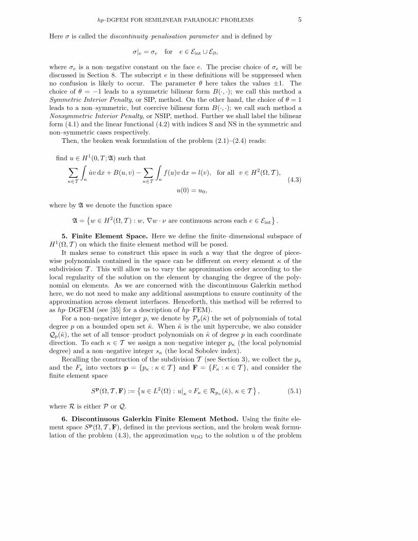
Here σ is called the discontinuity–penalisation parameter and is defined by

σ|e = σe for e ∈ Eint ∪ E∂ ,

where σe is a non–negative constant on the face e. The precise choice of σe will bediscussed in Section 8. The subscript e in these definitions will be suppressed whenno confusion is likely to occur. The parameter θ here takes the values ±1. Thechoice of θ = −1 leads to a symmetric bilinear form B(·, ·); we call this method aSymmetric Interior Penalty, or SIP, method. On the other hand, the choice of θ = 1leads to a non–symmetric, but coercive bilinear form B(·, ·); we call such method aNonsymmetric Interior Penalty, or NSIP, method. Further we shall label the bilinearform (4.1) and the linear functional (4.2) with indices S and NS in the symmetric andnon–symmetric cases respectively.

Then, the broken weak formulation of the problem (2.1)–(2.4) reads:

find u ∈ H1(0, T ;A) such that∑

κ∈T

∫

κ

uv dx + B(u, v) −∑

κ∈T

∫

κ

f(u)v dx = l(v), for all v ∈ H2(Ω, T ),

u(0) = u0,

(4.3)

where by A we denote the function space

A =w ∈ H2(Ω, T ) : w, ∇w · ν are continuous across each e ∈ Eint

.

5. Finite Element Space. Here we define the finite–dimensional subspace ofH1(Ω, T ) on which the finite element method will be posed.

It makes sense to construct this space in such a way that the degree of piece-wise polynomials contained in the space can be different on every element κ of thesubdivision T . This will allow us to vary the approximation order according to thelocal regularity of the solution on the element by changing the degree of the poly-nomial on elements. As we are concerned with the discontinuous Galerkin methodhere, we do not need to make any additional assumptions to ensure continuity of theapproximation across element interfaces. Henceforth, this method will be referred toas hp–DGFEM (see [35] for a description of hp–FEM).

For a non–negative integer p, we denote by Pp(κ) the set of polynomials of totaldegree p on a bounded open set κ. When κ is the unit hypercube, we also considerQp(κ), the set of all tensor–product polynomials on κ of degree p in each coordinatedirection. To each κ ∈ T we assign a non–negative integer pκ (the local polynomialdegree) and a non–negative integer sκ (the local Sobolev index).

Recalling the construction of the subdivision T (see Section 3), we collect the pκ

and the Fκ into vectors p = pκ : κ ∈ T and F = Fκ : κ ∈ T , and consider thefinite element space

Sp(Ω, T ,F) :=u ∈ L2(Ω) : u|κ Fκ ∈ Rpκ

(κ), κ ∈ T

, (5.1)

where R is either P or Q.

6. Discontinuous Galerkin Finite Element Method. Using the finite ele-ment space Sp(Ω, T ,F), defined in the previous section, and the broken weak formu-lation of the problem (4.3), the approximation uDG to the solution u of the problem


(2.1)–(2.4), discretised by the discontinuous Galerkin finite element method in space,is defined as follows:

find uDG ∈ H1(0, T ;Sp(Ω, T ,F)) such that∑

κ∈T

∫

κ

uDGv dx + B(uDG, v) −∑

κ∈T

∫

κ

f(uDG)v dx = l(v), for all v ∈ Sp(Ω, T ,F),

uDG(0) = uDG0 ,

(6.1)

where uDG0 denotes the approximation of the function u0 from the finite element

space Sp(Ω, T ,F), and the parameter σ in (4.1) and (4.2) is to be defined in the erroranalysis.

The equation (6.1) can be interpreted as a system of ordinary differential equationsin t for the coefficients in the expansion of uDG(t) in terms of basis functions of thefinite–dimensional space Sp(Ω, T ,F). Thus, (6.1) defines an autonomous system ofordinary differential equations with C1 (and, therefore, locally Lipschitz continuous)right–hand side, given that f ∈ C1(R) and the other terms are linear. By the Cauchy–Picard theorem this, in turn, implies the existence of a unique local solution to (6.1).

Since no pointwise continuity requirement is imposed on the elements of the finiteelement space, the approximation uDG in Sp(Ω, T ,F) to the solution u will be, ingeneral, discontinuous.

Remark 6.1 If the continuity assumptions made in the construction of the space A

are violated, i.e., u and ∇u ·ν are discontinuous across the element interfaces, we haveto modify the DGFEM accordingly. This could be done, for example, by performing aDGFEM discretisation on every subdomain of Ω where the continuity requirements aresatisfied, and incorporating into the definition of the method transmission conditionson interfaces where discontinuities in the solutions occur. Such situations include,for example, heat transfer problems in heterogeneous or layered media or problemsthat contain different phases of material. There the solution u and/or the diffusivefluxes ∇u·n can be discontinuous across element interfaces. This information has to beincorporated into the definition of the method and, in particular, into the choice of thediscontinuity–penalisation parameter σ, to avoid penalising physical discontinuities.

2

7. hp–Error Estimates. The first analysis of the p–version of FEM for Poisson’sequation was given by Babuska et al. [9], and was subsequently refined by Babuska& Suri in [7] and [8]. The analysis relied on the use of the Babuska–Suri projectionoperator. For the special case of n = 2, the analysis in W s

q –norms was carried outby Ainsworth & Kay in [2] and [3], where the approximation bounds were used forderiving a priori error bounds for p– and hp–version FEMs for the r–Laplacian, usingapproximation by continuous piecewise polynomials on both quadrilateral and trian-gular elements. The error bounds obtained in these works contain logarithmic termsin p, and thus are only optimal in p up to a logarithmic factor.

We shall proceed with the derivation of local approximation error bounds, avoid-ing such suboptimal logarithmic terms by using some very recent results due to Melenk[28].

From Proposition A.2 and Theorem A.3 in [28], we conclude the following resultconcerning polynomial approximation of functions defined on hypercubes.


Lemma 7.1 Let Q := (−1, 1)n, n ≥ 1, and let u ∈ W kq (Q), where q ∈ [1,∞]; then

there exists a sequence of algebraic polynomials zp(u) ∈ Rp(Q), p ∈ N, such that, forany 0 ≤ l ≤ k,

‖u − zp(u)‖W lq(Q) ≤ Cp−(k−l) ‖u‖W k

q (Q) , 1 ≤ q ≤ ∞, (7.1)

where C > 0 is a constant, independent of u and p, but dependent on q and k.

To derive the general hp–estimates for the projection operator u 7→ zp(u), recallfrom Sections 3 and 5 the construction of the subdivision T of the computationaldomain Ω. Let κ be the n–dimensional open unit hypercube, which we shall call thereference element. We construct each element κ ∈ T via an affine mapping fromthe reference element κ = Fκ(κ), based on scaling each coordinate of the referenceelement by the factor hκ.

We shall also need the following result.

Lemma 7.2 Suppose that κ ∈ T is an n–dimensional parallelepiped of diameter hκ,and that u|κ ∈ W kκ

q (κ) for some kκ ≥ 0 and κ ∈ T . Define u ∈ W kκq (κ) by the rule

u(x)|κ = u(Fκ(x))|κ; Then

infv∈Rpκ (κ)

‖u − v‖W kκq (κ) ≤ Chsκ−n/q

κ ‖u‖W kκq (κ) ,

where sκ = min(pκ + 1, kκ).

Proof. (See [7], Lemma 4.4, and [3], Lemma 1). Assume that kκ is an integer.If kκ = 0, then the result follows by bounding the left–hand side of the inequalityby ‖u‖Lq(κ) and scaling to ‖u‖Lq(κ). Suppose, therefore, that kκ ≥ 1. For any

v ∈ Rpκ(κ), we have

‖u − v‖W kκq (κ) ≤ ‖u − v‖W sκ

q (κ) +

kκ∑

lκ=sκ+1

|u|W lκq (κ) ,

with the convention that if sκ = kκ then the summation is over an empty index setof lκ.

Using Theorem 3.1.1 in [12], we obtain

infv∈Rpκ (κ)

‖u − v‖W kκq (κ) ≤

kκ∑

lκ=sκ

|u|W lκq (κ) .

Scaling back to the element κ ∈ T , we obtain the result for integer kκ. The result forgeneral kκ follows by a standard function space interpolation argument.

2

Now we are ready to state our main result concerning the approximation proper-ties of the projection operator u 7→ zp(u).

Theorem 7.3 Suppose that κ ∈ T is an n–dimensional parallelepiped of diameter hκ,and that u|κ ∈ W kκ

q (κ) for some kκ ≥ 0 and κ ∈ T ; then, there exists a sequence of

algebraic polynomials zhκpκ

(u) ∈ Rpκ(κ), pκ ≥ 1, such that for any l, with 0 ≤ l ≤ kκ,

∥∥u − zhκ

pκ(u)

∥∥W l

q(κ)≤ C

hsκ−lκ

pkκ−lκ

‖u‖W kκq (κ) , 1 ≤ q ≤ ∞, (7.2)


and, for q = 2,

∥∥u − zhκ

pκ(u)

∥∥L2(eκ)

≤ Ch

sκ−12

κ

pkκ−

12

κ

‖u‖Hkκ (κ) , (7.3)

∥∥∇(u − zhκ

pκ(u))

∥∥L2(eκ)

≤ Ch

sκ−32

κ

pkκ−

32

κ

‖u‖Hkκ (κ) , (7.4)

where eκ is any face (edge) eκ ⊂ ∂κ, sκ = min(pκ + 1, kκ), and C is a constantindependent of u, hκ, and pκ, but dependent on k = maxκ∈T kκ and q.

Proof. (See also [7]). Let u ∈ W kκq (κ) and define u ∈ W kκ

q (κ) by the rule u(x)|κ =u(Fκ(x))|κ. First, we note that, by Lemma 4.1 in [7], for any v ∈ Rpκ

(κ), we have

the property that zhκpκ (v) = v. By Lemma 7.1, (7.1), we have, for 0 ≤ l ≤ kκ,∥∥∥∥u − zhκ

pκ (u)

∥∥∥∥W l

q(κ)

≤ Cp−(kκ−l)κ ‖u‖W kκ

q (κ) .

Noting that zhκpκ (u)(x) = zhκ

pκ(u)(Fκ(x)), and applying Lemma 7.2 with v ∈ Rpκ

(κ),we obtain

∥∥∥∥u − zhκpκ (u)

∥∥∥∥W l

q(κ)

=

∥∥∥∥(u − v) − zhκpκ (u − v)

∥∥∥∥W l

q(κ)

≤ Cp−(kκ−l)κ inf

v∈Rpκ (κ)‖u − v‖W kκ

q (κ) ≤ Cp−(kκ−l)κ h

sκ−nq

κ ‖u‖W kκq (κ) .

Thus, by a scaling argument, for 0 ≤ m ≤ l ≤ kκ, we have∣∣u − zhκ

pκ(u)

∣∣W m

q (κ)≤ Cp−(kκ−l)

κ hsκ−mκ ‖u‖W kκ

q (κ) ,

and therefore∥∥u − zhκ

pκ(u)

∥∥W l

q(κ)≤ Cp−(kκ−l)

κ hsκ−lκ ‖u‖W kκ

q (κ) ,

and hence (7.2).By setting q = 2 in (7.2) and using the trace inequality

‖u‖L2(∂κ) ≤ C(h− 1

2κ ‖u‖L2(κ) + ‖u‖

12

L2(κ) ‖∇u‖12

L2(κ)

),

we obtain (7.3) and (7.4).2

8. Error Analysis. This section is be concerned with the derivation of a pri-ori error bounds for the initial–boundary value problem for the semilinear parabolicequation described in Section 2.

We shall assume that the polynomial degree vector p, with pκ ≥ 1 for each κ ∈ T ,has bounded local variation, i.e., there exists a constant ρ ≥ 1 such that, for any pairof elements κ and κ′ which share an (n − 1)–dimensional face,

ρ−1 ≤ pκ

pκ′

≤ ρ. (8.1)


We also recall our regularity assumptions on the subdivision T : namely, T isshape–regular, and regular or 1–irregular. We shall consider the error analysis ofthe hp–version of the discontinuous Galerkin finite element method on shape–regularmeshes. In particular, we shall derive a priori error bounds for both the symmetricand the non–symmetric version of DGFEM.

Let us begin with the following lemma which establishes the local Lipschitz con-tinuity of the non–linearity f , required in the a priori error analysis of the hp–versionof DGFEM (6.1) for the model problem (2.1)–(2.4).

Lemma 8.1 Let f ∈ C1(R) satisfy the growth–condition (2.2) with 0 < α < ∞ whenn = 2 and 0 < α ≤ 2/(n − 2) when n ≥ 3, and suppose that 2 < q < ∞. Let

q = max

(q,

2αq

q − 2

).

Then, there exists a positive constant C = C(α,Cg, q, |Ω|) such that

‖f(u) − f(v)‖L2(Ω) ≤ C ‖u − v‖Lq(Ω)

(1 + ‖u‖α

L2αqq−2 (Ω)

+ ‖v‖α

L2αqq−2 (Ω)

)(8.2)

for all u, v ∈ Lq(Ω).Suppose that q = 2(α + 1); then q = 2(α + 1). Moreover, if n = 2, 0 < α < ∞

then 2 < q < ∞, and if n ≥ 3, 0 < α ≤ 2/(n − 2) then 2 < q ≤ 2n/(n − 2).

Proof. From (2.2), by Holder’s inequality, we have

‖f(u) − f(v)‖2L2(Ω) =

∫

Ω

|f(u) − f(v)|2 dx ≤ C2g

∫

Ω

(u − v)2(1 + |u| + |v|)2α dx

≤ C2g

(∫

Ω

|u − v|2·q

2 dx

) 2q

(∫

Ω

(1 + |u| + |v|)2α·(1− 2q )

−1

dx

)1− 2q

.

As 1 − 2/q = (q − 2)/q and q > 2, we have

‖f(u) − f(v)‖2L2(Ω) ≤ C2

g

(∫

Ω

|u − v|q dx

) 2q

(∫

Ω

(1 + |u| + |v|)2αq

q−2 dx

) q−2q

= C2g ‖u − v‖2

Lq(Ω)

(∫

Ω

(1 + |u| + |v|)2αq

q−2 dx

) q−2q

= C2g ‖u − v‖2

Lq(Ω)

(∫

Ω

(1 + |u| + |v|)2αq

q−2 dx

) q−22αq

·2α

≤ C2g ‖u − v‖2

Lq(Ω)

(|Ω|

q−22αq + ‖u‖

L2αqq−2 (Ω)

+ ‖v‖L

2αqq−2 (Ω)

)2α

≤ C2 ‖u − v‖2Lq(Ω)

(1 + ‖u‖α

L2αqq−2 (Ω)

+ ‖v‖α

L2αqq−2 (Ω)

)2

,

and hence (8.2) for all u, v ∈ Lq(Ω). The statement in the final sentence of the lemmafollows from our hypothesis on the range of α and the fact that q = 2(α + 1).

2

Hypothesis A. Let f ∈ C1(R) satisfy the growth–condition (2.2) with 0 < α < ∞when n = 2, and 0 < α ≤ 2/(n − 2) when n ≥ 3. We define q = 2(α + 1).


With this hypothesis in mind, we can remove the dependence on q in the constantC in Lemma 8.1 in terms of α.

For the sake of clarity of the exposition, in the rest of the paper we shall confineourselves to the case of n ≥ 3. Our proofs can be easily adjusted to cover the case ofn = 2 with 0 < α < ∞.

8.1. The Non–Symmetric Version of DGFEM. Let the bilinear form B beas in (4.1). Here we shall be concerned with the non–symmetric version of DGFEMcorresponding to θ = 1 in (4.1), so we write BNS(·, ·) in place of B(·, ·). We begin ourerror analysis with the following definition.

Definition 8.2 We define the quantity |‖·|‖DG on H1(Ω, T ), associated with theDGFEM, as follows:

|‖w|‖DG :=

(∑

κ∈T

‖∇w‖2L2(κ) +

∫

ΓD

σw2 ds +

∫

Γint

σ [w]2

ds

) 12

, (8.3)

where σ is a non–negative function on Γ.

Remark 8.3 Let us observe some properties of |‖·|‖DG defined above.1. If σ > 0 on Γ, then |‖·|‖DG defines a norm in H1(Ω, T ).2. If σ = 0 on Γ, then |‖·|‖DG defines a seminorm in H1(Ω, T ).3. Clearly, |‖w|‖2

DG = BNS(w,w), for all w ∈ H1(Ω, T ).2

The first step in the error analysis is to decompose the error u − uDG, where udenotes the analytical solution, as u−uDG = ξ +η, where ξ ≡ Πu−uDG, η ≡ u−Πu,with Π defined element–wise by

(Πu)|κ := Π(u|κ),

and Π denoting an appropriate projection operator on the element κ. Thus, using thetriangle inequality for the H1–norm, we have

‖u − uDG‖H1(Ω,T ) ≤ ‖η‖H1(Ω,T ) + ‖ξ‖H1(Ω,T ) . (8.4)

We assume for simplicity that the initial value is chosen as

uDG0 = Πu0, (8.5)

and thus ξ(0) = 0.We shall proceed by deriving a bound on ‖ξ‖H1(Ω,T ) in terms of norms of η. Then,

by choosing a suitable projection operator Π, we shall be able to use the bounds onvarious norms of the projection error η derived in Section 7 to deduce an a priorierror bound for the method.

Let us prove the continuity of the bilinear form BNS, which will also provide thenecessary bound for our error analysis.

Lemma 8.4 Let T be a shape–regular subdivision of Ω and assume that the parameterσ is positive on Γint ∪ ΓD; then, the following inequality holds for all v ∈ H1(Ω, T )


and w ∈ Sp(Ω, T ,F), with C a positive constant that depends only on the dimensionn and the shape–regularity of T :

|BNS(v, w)| ≤ C |‖w|‖DG

∫

ΓD

σ |v|2 ds +

∫

Γint

σ [v]2

ds +∑

κ∈T

‖∇v‖2L2(κ)

+∑

κ∈T

(∥∥√τv

∥∥2

L2(∂κ∩ΓD)+

∥∥∥∥1√σ∇v

∥∥∥∥2

L2(∂κ∩ΓD)

)

+∑

κ∈T

(∥∥√τ [v]

∥∥2

L2(∂κ∩Γint)+

∥∥∥∥1√σ∇v

∥∥∥∥2

L2(∂κ∩Γint)

) 12

,

(8.6)where τe =

⟨p 2

⟩e/he and he is the diameter of a face e ⊂ Eint ∪ ED; when e ∈ ED the

contribution from outside Ω in the definition of τe is set to 0.

Proof. (See also [21].) Let us decompose

|BNS(v, w)| ≤ I + II + III + IV,

where

I ≡∣∣∣∣∣∑

κ∈T

∫

κ

∇v · ∇w dx

∣∣∣∣∣ , II ≡∣∣∣∣∫

ΓD

v(∇w · n) − (∇v · n)w ds

∣∣∣∣ ,

III ≡∣∣∣∣∫

Γint

[v] 〈∇w · ν〉 − 〈∇v · ν〉 [w] ds

∣∣∣∣ ,

IV ≡∣∣∣∣∫

ΓD

σvw ds +

∫

Γint

σ [v] [w] ds

∣∣∣∣ .

For the term I we have

I ≤ |‖w|‖DG

∑

κ∈T

(‖∇v‖2

L2(κ)

) 12

, (8.7)

and for the term IV we have that

IV ≤ |‖w|‖DG

(∫

ΓD

σ |v|2 ds +

∫

Γint

σ [v]2

ds

) 12

. (8.8)

To deal with the term II, we first note that

II ≤(∑

κ∈T

1

γκ‖v‖2

L2(∂κ∩ΓD)

) 12

(∑

κ∈T

γκ ‖∇w‖2L2(∂κ∩ΓD)

) 12

+

(∑

κ∈T

∥∥∥∥1√σ∇v

∥∥∥∥2

L2(∂κ∩ΓD)

) 12

(∑

κ∈T

∥∥√σ w∥∥2

L2(∂κ∩ΓD)

) 12

for any set of positive numbers γκ : κ ∈ T . Here we can apply the inverse inequality

‖∇w‖2L2(∂κ∩ΓD) ≤ K

p2κ

hκ‖∇w‖2

L2(κ) , (8.9)


where K depends only on the shape–regularity of T (see Schwab [35], Theorem 4.76,(4.6.4)). On letting γκ = hκ/p2

κ and defining τe = p2κ/2he for an (n − 1)–dimensional

face e ⊂ ∂κ ∩ ΓD, we obtain

II ≤ C|‖w|‖DG

∑

κ∈T

(∥∥√τv

∥∥2

L2(∂κ∩ΓD)+

∥∥∥∥1√σ∇v

∥∥∥∥2

L2(∂κ∩ΓD)

) 12

. (8.10)

Similarly, we have

III ≤ C|‖w|‖DG

∑

κ∈T

(∥∥√τ [v]

∥∥2

L2(∂κ∩Γint)+

∥∥∥∥1√σ∇v

∥∥∥∥2

L2(∂κ∩Γint)

) 12

. (8.11)

By collecting the results we have the desired bound.2

Now, let us derive a bound on the H1–norm of the error u − uDG.

Lemma 8.5 Let T be a shape–regular subdivision of Ω and assume that f ∈ C1(R)satisfies Hypothesis A. Suppose further that the positive parameter σ is defined onΓint ∪ ΓD and

σe = σ|e ≥ h−1e

on each face e ∈ Eint ∪ ED. In addition, suppose thata) the local polynomial degree pκ ≥ 2 on each κ ∈ T ;b) the local Sobolev smoothness kκ ≥ 3.5 on each κ ∈ T ;c) the hp–mesh is quasi–uniform in the sense that there exists a positive constant

C0 such that

maxκ∈T

hκ

p2κ

≤ C0 minκ∈T

hκ

p2κ

.

Then, for all t ∈ [0, T ], there exists h0 > 0 such that for all h ∈ (0, h0], h =maxκ∈T hκ, the following inequality holds, with C a positive constant that dependsonly on the domain Ω, the quasi–uniformity of T , on the final time T , the exponentα in the growth–condition for the function f , and the Lebesgue and Sobolev norms ofu over the time interval [0, T ]:

∫ t

0

‖(u − uDG)(s)‖2H1(Ω,T ) ds ≤ C

∑

κ∈T

∫ t

0

‖η(s)‖2

L2(κ) + ‖η(s)‖2L2(α+1)(κ) + ‖η(s)‖2

H1(κ)

+∥∥√ση(s)

∥∥2

L2(∂κ∩ΓD)+

∥∥√σ [η(s)]∥∥2

L2(∂κ∩Γint)+

∥∥√τη(s)∥∥2

L2(∂κ∩ΓD)

+

∥∥∥∥1√σ∇η(s)

∥∥∥∥2

L2(∂κ∩ΓD)

+∥∥√τ [η(s)]

∥∥2

L2(∂κ∩Γint)+

∥∥∥∥1√σ∇η(s)

∥∥∥∥2

L2(∂κ∩Γint)

ds

(8.12)

where τe =⟨p2

⟩e/he and he is the diameter of a face e ∈ Eint ∪ ED, in which for

e ∈ ED the contribution from outside Ω is set to 0.

Proof. From the formulation of the hp–DGFEM (6.1), for all v ∈ Sp(Ω, T ,F),we have

∑

κ∈T

∫

κ

uDGv dx + BNS(uDG, v) =∑

κ∈T

∫

κ

f(uDG)v dx + lNS(v). (8.13)


On the other hand, the broken weak formulation (4.3) of the problem can be rewrittenas

∑

κ∈T

∫

κ

(Πu)v dx + BNS(Πu, v) =∑

κ∈T

∫

κ

f(u)v dx + lNS(v)

+∑

κ∈T

∫

κ

(Πu − u)v dx + BNS(Πu − u, v).

(8.14)

Upon subtracting (8.13) from (8.14) and choosing v = ξ, we obtain

∑

κ∈T

∫

κ

ξξ dx + BNS(ξ, ξ) =∑

κ∈T

∫

κ

f(u) − f(uDG) ξ dx −∑

κ∈T

∫

κ

ηξ dx − BNS(η, ξ).

By noting that

∑

κ∈T

∫

κ

ξξ dx =1

2

d

dt

∑

κ∈T

‖ξ‖2L2(κ) =

1

2

d

dt‖ξ‖2

L2(Ω) ,

we can rewrite the above expression as

1

2

d

dt‖ξ‖2

L2(Ω)+|‖ξ|‖2DG ≤

∣∣∣∣∣∑

κ∈T

∫

κ

f(u) − f(Πu) ξ dx

∣∣∣∣∣+∣∣∣∣∣∑

κ∈T

∫

κ

f(Πu) − f(uDG) ξ dx

∣∣∣∣∣

+

∣∣∣∣∣∑

κ∈T

∫

κ

ηξ dx

∣∣∣∣∣ + |BNS(η, ξ)| . (8.15)

By the Cauchy–Schwarz and Young inequalities, with ε1 > 0, we have

∣∣∣∣∣∑

κ∈T

∫

κ

ηξ dx

∣∣∣∣∣ ≤(∑

κ∈T

‖η‖2L2(κ)

) 12

(∑

κ∈T

‖ξ‖2L2(κ)

) 12

≤ ε1

2‖η‖2

L2(Ω) +1

2ε1‖ξ‖2

L2(Ω) ,

and, by the same argument, with ε2, ε3 > 0,∣∣∣∣∣∑

κ∈T

∫

κ

f(u) − f(Πu) ξ dx

∣∣∣∣∣ ≤ε2

2‖f(u) − f(Πu)‖2

L2(Ω) +1

2ε2‖ξ‖2

L2(Ω) ,

∣∣∣∣∣∑

κ∈T

∫

κ

f(Πu) − f(uDG) ξ dx

∣∣∣∣∣ ≤ε3

2‖f(Πu) − f(uDG)‖2

L2(Ω) +1

2ε3‖ξ‖2

L2(Ω) .

Further, by Lemma 8.1, upon absorbing all constants into C and noting the definitionof q in Hypothesis A, we have

‖f(u) − f(Πu)‖2L2(Ω) ≤ C ‖η‖2

Lq(Ω)

(1 + ‖u‖α

L2αqq−2 (Ω)

+ ‖Πu‖α

L2αqq−2 (Ω)

)2

≤ C ‖η‖2Lq(Ω)

(1 + ‖u‖2α

L2αqq−2 (Ω)

+ ‖Πu‖2α

L2αqq−2 (Ω)

)

= C ‖η‖2Lq(Ω)

(1 + ‖u‖2α

L2αqq−2 (Ω)

+ ‖u − η‖2α

L2αqq−2 (Ω)

)

≤ C ‖η‖2Lq(Ω)

(1 + ‖u‖2α

L2αqq−2 (Ω)

+ ‖η‖2α

L2αqq−2 (Ω)

)

≤ C ‖η‖2Lq(Ω) = C ‖η‖2

L2(α+1)(Ω) ,


where the constant C > 0 depends only on the domain Ω, the growth–condition forthe function f , and on Lebesgue norms of u over the time interval [0, T ].

By Lemma 8.4 and Young inequality, with ε4 > 0, we have the bound

|BNS(η, ξ)| ≤ ε4

2|‖ξ|‖2

DG +1

2ε4F1(η),

where

F1(η) := C∑

κ∈T

(‖∇η(s)‖2

L2(κ) +∥∥√ση(s)

∥∥2

L2(∂κ∩ΓD)+

∥∥√σ [η(s)]∥∥2

L2(∂κ∩Γint)

+∥∥√τη(s)

∥∥2

L2(∂κ∩ΓD)+

∥∥∥∥1√σ∇η(s)

∥∥∥∥2

L2(∂κ∩ΓD)

+∥∥√τ [η(s)]

∥∥2

L2(∂κ∩Γint)+

∥∥∥∥1√σ∇η(s)

∥∥∥∥2

L2(∂κ∩Γint)

).

Applying these bounds on the right–hand side of (8.15) and absorbing all con-stants into C1 and C2, we obtain

d

dt‖ξ‖2

L2(Ω)+(2−ε4)|‖ξ|‖2DG ≤ C1F(η)+C2 ‖ξ‖2

L2(Ω)+ε3 ‖f(Πu) − f(uDG)‖2L2(Ω) ,

(8.16)

where

F(η) := F1(η) + ‖η‖2L2(α+1)(Ω) + ‖η‖2

L2(Ω) .

To bound ‖f(Πu) − f(uDG)‖2L2(Ω), we first note that, by the same argument as

above,

‖f(Πu) − f(uDG)‖2L2(Ω) ≤ C ‖ξ‖2

L2(α+1)(Ω)

(1 + ‖uDG‖2α

L2αqq−2 (Ω)

),

where the constant C > 0 depends only on the domain Ω, the growth–condition forthe function f , and on Lebesgue norms of u over the time interval [0, T ].

Let us choose uDG0 = Πu0, thus giving ξ(0) = 0, and let 0 < t⋆ ≤ T be the largest

time such that uDG exists for all t ∈ [0, t⋆] and

‖ξ‖2H1(Ω,T ) ≤ 1 for all t ∈ [0, t⋆];

existence of such a t⋆ is guaranteed by the Cauchy–Picard theorem. Since, by Hy-pothesis A, 2αq/(q − 2) ≤ 2n/(n − 2), this implies that

‖uDG‖2α

L2αqq−2 (Ω)

≤ Const. for all t ∈ [0, t⋆]

by the broken Sobolev–Poincare inequality (see Theorem 3.7 in [27]1); here Const.is a constant that is independent of the discretisation parameters and t, and only

1Using the notation of the cited paper, we define Ψ as in Example 3.6 of that paper, with

ψ ∈ L2(∂Ω), ψ ≡ 0 on ΓN

and

|Ψ(ξ)|2 ≤ C∑

e∈ED

h−1

e

∫

e

ξ2 ds.


depends on Sobolev norms of u over the time interval [0, t⋆].This implies that

‖f(Πu) − f(uDG)‖2L2(Ω) ≤ C|‖ξ|‖2

DG,

where the constant C > 0 depends only on the domain Ω, the growth–condition forthe function f , and on Lebesgue and Sobolev norms of u over the time interval [0, t⋆].

On choosing ε4 + ε3C ≤ 1, (8.16) takes the form

d

dt‖ξ‖2

L2(Ω) + |‖ξ|‖2DG ≤ C1F(η) + C2 ‖ξ‖2

L2(Ω) , (8.17)

with the constant C1 > 0 depending only on the domain Ω, the growth–condition forthe function f , and on Lebesgue and Sobolev norms of u over the time interval [0, t⋆].

Upon integrating from 0 to t ≤ t⋆ and noting that ξ(0) = 0, this yields

‖ξ(t)‖2L2(Ω) +

∫ t

0

|‖ξ(s)|‖2DG ds ≤ C1

∫ t

0

F(η(s)) ds + C2

∫ t

0

‖ξ(s)‖2L2(Ω) ds, (8.18)

with the constant C1 as above.

According to this inequality, if F(η) were zero, we would have ‖ξ‖2L2(Ω) = 0 for

all t ∈ [0, t⋆]. More generally, by choosing an appropriate projection operator Π, wecan make F(η) as small as we like (for example, by fixing the local polynomial degreepκ on each element κ ∈ T and reducing h = maxκ∈T hκ).

Let us choose C3 = C222α and h0 > 0 so small that, for all h ≤ h0 and t ∈ [0, t⋆],

the following inequality holds:

C1

∫ t

0

F(η(s)) ds <1

1 + Te−C3T × C−1

invC−20

(maxκ∈T

hκ

p2κ

)2

,

where Cinv is the constant from the inverse inequality

‖ξ‖2H1(Ω,T ) ≤ Cinv

(maxκ∈T

p2κ

hκ

)2

‖ξ‖2L2(Ω) . (8.19)

We note in passing that in order to be able to extract the factor (maxκ∈T (hκ/p2κ))2

from F(η), we need hypotheses a) and b) above.Hence (8.18) becomes

‖ξ(t)‖2L2(Ω) +

∫ t

0

|‖ξ(s)|‖2DG ds <

1

1 + Te−C3T × C−1

invC−20

(maxκ∈T

hκ

p2κ

)2

+ C2

∫ t

0

‖ξ(s)‖2L2(Ω) ds,

which, by the Gronwall–Bellman inequality, implies that

‖ξ(t)‖2L2(Ω) < C−1

invC−20

(maxκ∈T

hκ

p2κ

)2

for all t ∈ [0, t⋆].

By the inverse inequality (8.19) we have that,

‖ξ(t)‖2H1(Ω,T ) < C−2

0

(maxκ∈T

hκ

p2κ

)2 (maxκ∈T

p2κ

hκ

)2

= C−20

(maxκ∈T

hκ

p2κ

)2 (minκ∈T

hκ

p2κ

)−2

,


for all t ∈ [0, t⋆], which, by the quasi–uniformity hypothesis c) above, is ≤ 1. Hence,then, for h ≤ h0, we have

‖ξ‖2H1(Ω,T ) < 1 for all t ∈ [0, t⋆].

By continuity of the mapping t 7→ ‖ξ(t)‖2H1(Ω,T ), the assumption t⋆ < T implies

that either ‖ξ(t)‖2H1(Ω,T ) ≤ 1 for all t ∈ [0, T ], or that there exists a time t⋆⋆ ∈ (t⋆, T ]

such that ‖ξ(t⋆⋆)‖2H1(Ω,T ) = 1.

In either case, we arrive at a contradiction with the fact that t⋆ is the largest timein the interval [0, T ] such that, for all t ∈ [0, t⋆], we have ‖ξ(t)‖2

H1(Ω,T ) ≤ 1. Thus wededuce that t⋆ = T , for 0 < h ≤ h0.

From (8.18) by the Gronwall–Bellman inequality we obtain

‖ξ(t)‖2L2(Ω) +

∫ t

0

‖ξ(s)‖2H1(Ω,T ) ds ≤ C

∫ t

0

F(η(s)) ds, 0 ≤ t ≤ T,

and hence

∫ t

0

‖ξ(s)‖2H1(Ω,T ) ds ≤ C

∫ t

0

F(η(s)) ds, 0 ≤ t ≤ T,

with the constant C > 0 depending only on the domain Ω, the quasi–uniformity of T ,on the time T , the growth–condition for the function f , and on Lebesgue and Sobolevnorms of u over the time interval [0, T ].

Employing the triangle inequality yields

∫ t

0

‖(u − uDG)(s)‖2H1(Ω,T ) ds ≤ C

∫ t

0

‖η‖2

H1(Ω,T ) + F(η(s))

ds, 0 ≤ t ≤ T,

and hence (8.12).2

Our next result concerns the accuracy of the hp–version NSIP DGFEM (6.1).

Theorem 8.6 Let Ω ⊂ Rn, n ≥ 2, be a bounded polyhedral domain, T = κ a

shape–regular and quasi–uniform subdivision of Ω into n–parallelepipeds, and p apolynomial degree vector of bounded local variation. Let each face e ∈ Eint ∪ ED beassigned a positive real number

σe =〈p〉ehe

, (8.20)

where he is the diameter of e, with the convention that for e ∈ ED the contributionsfrom outside Ω in the definition of σe are set to 0. Suppose that the function f ∈C1(R), that f satisfies the growth–condition (2.2) for some positive constant Cg, andthat Hypothesis A holds. Then, if u(·, t)|κ ∈ Hkκ(κ) with kκ ≥ 3.5 on each κ ∈ T ,there exists h0 > 0 such that for all h ∈ (0, h0], h = maxκ∈T hκ, and all t ∈ [0, T ],the solution uDG(·, t) ∈ Sp(Ω, T ,F) of the NSIP DGFEM (6.1) satisfies the followingerror bound:

‖u − uDG‖2L2(0,T ;H1(Ω,T )) ≤ C

∑

κ∈T

h2sκ−2κ

p2kκ−3κ

‖u‖2X

; (8.21)


with 1 ≤ sκ ≤ min(pκ + 1, kκ), pκ ≥ 2 on each κ ∈ T , where C is a positive constantdepending only on the domain Ω, the shape–regularity and quasi–uniformity of T , thetime T , the growth–condition on the function f , the parameter ρ in (8.1), on k =maxκ∈T kκ, and on the Lebesgue and Sobolev norms of u over the time interval [0,T];

the norm ‖u‖2X

signifies the collection of norms ‖u‖2L2(0,T ;Hkκ (κ))+‖u‖2

L2(0,T ;Hkκ−1(κ)).

Proof. Let us choose the projector Π to be the projection operator u 7→ zhκpκ

(u),defined in Section 7. From Theorem 7.3, inequalities (7.2)–(7.4), we have the estimates

‖η‖2L2(∂κ) ≤ C

h2sκ−1κ

p2kκ−1κ

‖u‖2Hkκ (κ) , ‖∇η‖2

L2(∂κ) ≤ Ch2sκ−3

κ

p2kκ−3κ

‖u‖2Hkκ (κ) ,

‖η‖2H1(κ) ≤ C

h2sκ−2κ

p2kκ−2κ

‖u‖2Hkκ (κ) , ‖η‖2

L2(κ) ≤ Ch2sκ

κ

p2kκκ

‖u‖2Hkκ (κ) .

Let us collect all the terms on the right–hand side of (8.12), except ‖η‖2L2(α+1)(κ):

I ≡ C∑

κ∈T

∫ t

0

‖η(s)‖2

L2(κ) + ‖η(s)‖2H1(κ) +

∥∥√ση(s)∥∥2

L2(∂κ∩ΓD)

+∥∥√σ [η(s)]

∥∥2

L2(∂κ∩Γint)+

∥∥√τη(s)∥∥2

L2(∂κ∩ΓD)+

∥∥∥∥1√σ∇η(s)

∥∥∥∥2

L2(∂κ∩ΓD)

+∥∥√τ [η(s)]

∥∥2

L2(∂κ∩Γint)+

∥∥∥∥1√σ∇η(s)

∥∥∥∥2

L2(∂κ∩Γint)

ds.

From the above approximation results, by choosing σe as in (8.20), noting (8.1) andthe shape–regularity of T to relate he to hκ, and taking the maximum over t ∈ [0, T ],we obtain

I ≤ C∑

κ∈T

h2sκ−2

κ

p2kκ−2κ

‖u‖2L2(0,T ;Hkκ−1(κ)) +

(h2sκ−2

κ

p2kκ−2κ

+p2

κ

hκ

h2sκ−1κ

p2kκ−1κ

)‖u‖2

L2(0,T ;Hkκ (κ))

≤ C∑

κ∈T

h2sκ−2κ

p2kκ−3κ

‖u‖2X

, (8.22)

with 1 ≤ sκ ≤ min(pκ + 1, kκ), pκ ≥ 2 on each κ ∈ T , where C is a positive constantdepending only on the domain Ω, the shape–regularity and quasi–uniformity of T ,the time T , the growth–condition for the function f , the parameter ρ in (8.1), onk = maxκ∈T kκ, and on the Lebesgue and Sobolev norms of u over the time interval[0, T ].

Further, by the broken Sobolev–Poincare inequality [27] we have the bound

‖η‖2L2(α+1)(Ω) ≤ C

(∑

κ∈T

‖∇η‖2L2(κ) +

∑

e∈Eint

h−1e

∫

e

[η]2

ds +∑

e∈ED

h−1e

∫

e

η2 ds

),

and thus by the above approximation bounds, by noting the shape–regularity of T torelate he to hκ, we obtain

∑

κ∈T

‖η‖2L2(α+1)(κ) ≤ C

∑

κ∈T

h2sκ−2κ

p2kκ−2κ

‖u‖2Hkκ (κ) ,


with the constant C as above.Applying this bound to the right–hand side of (8.12), noting (8.22), and taking

the maximum over 0 ≤ t ≤ T , we obtain the desired bound.2

Remark 8.7

1. The estimate (8.21) is optimal in h and p–suboptimal by p12 .

2. By the broken Sobolev–Poincare inequality, the same bound holds for theL2–norm of the error. The bound in this case is not hp–optimal.

3. From the error bound we conclude that the presence of the non–linearity f(·),satisfying the conditions stated in Section 2, does not diminish the rate ofhp–convergence rate in the H1–norm compared to the linear case.

2

8.2. The Symmetric Version of DGFEM. The symmetric version of theinterior penalty discontinuous Galerkin finite element method appeared in the liter-ature much earlier than the non–symmetric formulation, (see Wheeler [36]). It wasnot widely accepted as an effective numerical method until very recently, due to anadditional condition on the size of the penalty parameter which is required in order toensure the coercivity of the bilinear form of the method; this will be discussed in thenext section. The renewed interest in the symmetric formulation of the IP DGFEM isdue to the optimality of its convergence rate in the L2–norm and for linear functionalsof the solution.

The non–symmetric formulation of the IP method suffers from lack of adjointconsistency (see [6, 5]), and results in suboptimal a priori error bounds in the L2–norm and in linear functionals of the solutions. The symmetric version, due to itsadjoint consistency, does not suffer from these drawbacks.

We start our a priori error analysis in the L2–norm by deriving the error boundson the broken elliptic projector defined by the symmetric version of the interior penaltydiscontinuous Galerkin finite element method. This part of the L2–norm error analysisis crucial, as it will allow us to remove the terms in the error bound, containing theH1–seminorm, which would otherwise result in a suboptimal convergence rate in theL2–norm.

8.2.1. The Broken Elliptic Projector. Consider the boundary value problemfor the elliptic equation in the form

−∆u = 0 in Ω,

u = gD on ΓD,

∇u · n = gN on ΓN,

(8.23)

with ΓD ∪ ΓN = ∂Ω, ΓD having positive measure, and gD ∈ H12 (ΓD), gN ∈ L2(ΓN).

We shall also assume that the solution u exists, that it is unique, and that u ∈ A.In view of Section 4, the SIP formulation of the DGFEM for this problem is

find uDG ∈ Sp(Ω, T ,F) such that BS(uDG, v) = lS(v) for all v ∈ Sp(Ω, T ,F),(8.24)

where the symmetric bilinear form BS is defined by (4.1), and the linear functional lSis defined by (4.2), with θ = −1.

Let us check whether and under what conditions the solution uDG to (8.24) existsand is unique.


The proof of continuity of the symmetric bilinear form BS(u, v) is essentially thesame as in the non–symmetric case (see Lemma 8.4). The coercivity, though, requiresfurther investigation.

For the symmetric bilinear form (4.1) (with θ = −1), we have, for any w ∈Sp(Ω, T ,F),

BS(w,w) =∑

κ∈T

‖∇w‖2L2(κ)+

∫

ΓD

(σw2 − 2w(∇w · n)

)ds+

∫

Γint

(σ [w]

2 − 2 [w] 〈∇w · ν〉)ds.

Clearly the integrands in the last two terms need not be positive unless σ is chosensufficiently large: the purpose of the analysis that now follows is to explore just howlarge σ needs to be to ensure coercivity of BS(·, ·) over Sp(Ω, T ,F) × Sp(Ω, T ,F).

For any positive number τe we have

−2

∫

ΓD

w(∇w · n) ds ≥ −∑

e∈ED

(∫

e

τew2 ds +

∫

e

τ−1e (∇w · n)2 ds

).

Omitting the summations, the second term on the right–hand side can be furtherbounded by using the inverse inequality (8.9), the shape–regularity condition (torelate hκ to he, where κ is the element whose face is e ∈ ED) and the bounded localvariation condition (to relate p2

κ to⟨p2

⟩e), by absorbing all constants into Cτ , we

obtain

−∫

e

τ−1e (∇w · n)2 ds ≥ −

∫

e

τ−1e |∇w|2 |n|2 ds ≥ −τ−1

e Cτ

⟨p2

⟩e

he‖∇w‖2

L2(κ) .

Similarly, for the term involving interior faces, we have

−2

∫

Γint

[w] 〈∇w · ν〉 ds ≥ −∑

e∈Eint

(∫

e

τe [w]2

ds + τ−1e Cτ

⟨p2

⟩e

he

(‖∇w‖L2(κ′) ‖∇w‖L2(κ′′)

)),

using the restriction imposed by the bounded local variation condition (8.1): here κ′

and κ′′ are the two elements that have e as their common face.Now letting

τ−1e :=

1

2n · 2n−1

(Cτ

⟨p2

⟩e

he

)−1

for e ∈ ED ∪ Eint,

we get

BS(w,w) ≥ 1

2

∑

κ∈T

‖∇w‖2L2(κ) +

∫

ΓD

(σ − τ)w2 ds +

∫

Γint

(σ − τ) [w]2

ds.

Thus the symmetric bilinear form BS(u, v) is coercive if

σe ≥ τe = 2n · 2n−1Cτ

⟨p2

⟩e

he.

The factor 2n · 2n−1 stems for the fact that in n dimensions the summation overe ∈ Eint may count, any one element κ, 2n · 2n−1 times, as we allow one hanging nodeper interface.


Choosing σe appropriately, i.e.,

σe = Cσ

⟨p2

⟩e

he(8.25)

with the constant Cσ > 0 large enough, σe ≥ τe will be ensured and by the Lax–Milgram theorem the solution to (8.24) then exists and is unique.

In view of the above arguments, we conclude that the SIP DGFEM solution of theproblem (8.23) uniquely determines the projection operator Πe on A onto the finiteelement space Sp(Ω, T ,F) with the property (for u ∈ A)

BS(u − Πeu, v) = 0 for all v ∈ Sp(Ω, T ,F). (8.26)

Next, we state the approximation error bounds in the H1– and L2–norms for thebroken elliptic projector Πe.

Lemma 8.8 Let Ω ⊂ Rn, n ≥ 2, be a bounded polyhedral domain, T = κ a shape–

regular subdivision of Ω into n–parallelepipeds, and suppose that u|κ ∈ Hkκ(κ) forsome Sobolev index kκ ≥ 2 and κ ∈ T . Let Πeu be the projection of u ∈ A ontoSp(Ω, T ,F), defined by (8.26), with pκ ≥ 0 for κ ∈ T , and σe chosen as in (8.25).Then, the following error estimate holds:

‖u − Πeu‖2H1(Ω,T ) ≤ C

∑

κ∈T

h2sκ−2κ

p2kκ−3κ

‖u‖2Hkκ (κ) . (8.27)

Furthermore, if Ω is convex, then

‖u − Πeu‖2L2(Ω) ≤ C

(maxκ∈T

h2κ

pκ

) ∑

κ∈T

h2sκ−2κ

p2kκ−3κ

‖u‖2Hkκ (κ) , (8.28)

where sκ = min(pκ + 1, kκ), and the constant C is independent of u, pκ and hκ, butdependent on k = maxκ∈T kκ and Cσ.

Proof. By recalling the definition of the DG–norm (8.3), we have, from the assump-tion on σe, that

|‖u|‖2DG ≤ BS(u, u) for all u ∈ A,

and thus by writing u − Πeu = (u − Πu)− (Πu − Πeu) = η + ξ, where the projectionoperator Π will be chosen later, taking v ≡ ξ in the definition of the broken ellipticprojector (8.26), we deduce that

|‖ξ|‖2DG ≤ BS(ξ + η − η, ξ) ≤ |BS(ξ + η, ξ)| + |BS(η, ξ)| = |BS(η, ξ)| .

By continuity of the bilinear form BS(η, ξ) (see Lemma 8.4 and the comments above),after applying Young inequality we have

|‖ξ|‖2DG ≤ C

∑

κ∈T

(∥∥√ση∥∥2

L2(∂κ∩ΓD)+

∥∥√σ [η]∥∥2

L2(∂κ∩Γint)+ ‖∇η‖2

L2(κ) +∥∥√τη

∥∥2

L2(∂κ∩ΓD)

+

∥∥∥∥1√σ∇η

∥∥∥∥2

L2(∂κ∩ΓD)

+∥∥√τ [η]

∥∥2

L2(∂κ∩Γint)+

∥∥∥∥1√σ∇η

∥∥∥∥2

L2(∂κ∩Γint)

), (8.29)


where τe = 2n · 2n−1Cτ

⟨p2

⟩e/he, he is the diameter of a face e ∈ Eint ∪ ED, and for

e ∈ ED the contribution from outside Ω is set to 0.Further, by noting that

∑κ∈T ‖∇ξ‖2

L2(κ) ≤ |‖ξ|‖2DG, and employing the triangle

inequality (8.4), we obtain the bound

∑

κ∈T

‖u − Πeu‖2H1(κ) ≤ C

∑

κ∈T

(∥∥√ση∥∥2

L2(∂κ∩ΓD)+

∥∥√σ [η]∥∥2

L2(∂κ∩Γint)+ ‖η‖2

H1(κ)

+∥∥√τη

∥∥2

L2(∂κ∩ΓD)+

∥∥∥∥1√σ∇η

∥∥∥∥2

L2(∂κ∩ΓD)

+∥∥√τ [η]

∥∥2

L2(∂κ∩Γint)+

∥∥∥∥1√σ∇η

∥∥∥∥2

L2(∂κ∩Γint)

), (8.30)

Let us choose Π to be the u 7→ zhκpκ

(u) (see Section 7). From Theorem 7.3,inequalities (7.2)–(7.4), we have the estimates

‖η‖2L2(∂κ) ≤ C

h2sκ−1κ

p2kκ−1κ

‖u‖2Hkκ (κ) , ‖∇η‖2

L2(∂κ) ≤ Ch2sκ−3

κ

p2kκ−3κ

‖u‖2Hkκ (κ) ,

‖η‖2H1(κ) ≤ C

h2sκ−2κ

p2kκ−2κ

‖u‖2Hkκ (κ) .

Applying these inequalities to the right–hand side of (8.30), choosing σe as in (8.25),noting the bounded local variation condition (8.1) and the shape regularity of T torelate he to hκ, we obtain

‖u − Πeu‖2H1(Ω,T ) ≤ C

∑

κ∈T

(h2sκ−2

κ

p2kκ−2κ

+p2

κ

hκ

h2sκ−1κ

p2kκ−1κ

)‖u‖2

Hkκ (κ) ,

and hence (8.27).Let us note that the same bound (8.27) is also valid for the DG–norm |‖u − Πeu|‖DG;

this follows from (8.29) and the fact that

|‖u − Πeu|‖2DG ≤ C

∑

κ∈T

h2sκ−2κ

p2kκ−3κ

‖u‖2Hkκ (κ) .

To estimate ‖u − Πeu‖L2(Ω), we shall use the Aubin–Nitsche duality argument

(see [11]).Let (·, ·) signify the L2–inner product. Then, for every g ∈ L2(Ω), by the Cauchy–

Schwarz inequality we have

(u − Πeu, g) ≤ ‖u − Πeu‖L2(Ω) ‖g‖L2(Ω) ,

and therefore

‖u − Πeu‖L2(Ω) = supg∈L2(Ω)

g 6=0

(u − Πeu, g)

‖g‖L2(Ω)

. (8.31)

Further, let the function w ∈ H2(Ω) be the solution of the problem

−∆w = g in Ω,

w = 0 on ΓD,

∇w · n = 0 on ΓN,

(8.32)


with g ∈ L2(Ω), and ΓD, ΓN as in (8.23). Then the SIP DGFEM formulation of thisproblem is

find w ∈ A such that BS(w, v) = lg(v) for all v ∈ H2(Ω, T ),

where BS(w, v) is defined by (4.1) with θ = −1, and

lg(v) = (g, v) + lS(v),

with lS(v) defined by (4.2) with θ = −1 and gD = 0, gN = 0: clearly, then, lS(v) = 0for all v in H2(Ω, T ).

Consider the SIP DGFEM approximation of (8.32) in the form

find wDG ∈ Sp(Ω, T ,F) such that BS(wDG, v) = lg(v) for all v ∈ Sp(Ω, T ,F).

By Galerkin orthogonality, we have

BS(u − Πeu,wDG) = 0,

and thence

(u − Πeu, g) = (g, u − Πeu) = lg(u − Πeu) = BS(w, u − Πeu)

= BS(u − Πeu,w) = BS(u − Πeu,w − Πw),

where Π is the projection operator u 7→ zhκpκ

(u).Further, by Lemma 8.4, (8.6), and by noting that the bilinear form BS(·, ·) is

symmetric, we have

(u−Πeu, g) ≤ BS(u − Πeu,w − Πw) ≤ C |‖u − Πeu|‖DG

×∫

ΓD

σ |w − Πw|2 ds +

∫

Γint

σ [w − Πw]2

ds +∑

κ∈T

‖∇(w − Πw)‖2L2(κ)

+∑

κ∈T

(∥∥√τ(w − Πw)

∥∥2

L2(∂κ∩ΓD)+

∥∥∥∥1√σ∇(w − Πw)

∥∥∥∥2

L2(∂κ∩ΓD)

)

+∑

κ∈T

(∥∥√τ [w − Πw]

∥∥2

L2(∂κ∩Γint)+

∥∥∥∥1√σ∇(w − Πw)

∥∥∥∥2

L2(∂κ∩Γint)

) 12

(8.33)with τe = 2n · 2n−1Cτ

⟨p2

⟩e/he.

By the previous argument, we have the estimate

|‖u − Πeu|‖2DG ≤ C

∑

κ∈T

h2sκ−2κ

p2kκ−3κ

‖u‖2Hkκ (κ) , (8.34)

and from Theorem 7.3, inequalities (7.2)–(7.4), we have the estimates

‖w − Πw‖2L2(∂κ) ≤ C

h3κ

p3κ

‖w‖2H2(κ) , ‖∇(w − Πw)‖2

L2(∂κ) ≤ Chκ

pκ‖w‖2

H2(κ) ,

‖∇(w − Πw)‖2L2(κ) ≤ C

h2κ

p2κ

‖w‖2H2(κ) .


Applying these inequalities and the estimate (8.34) to the right–hand side of (8.33),choosing σe as in (8.25) and noting the bounded local variation condition (8.1) andthe shape regularity of T to relate he to hκ, we obtain

(u − Πeu, g) ≤ C

(∑

κ∈T

h2sκ−2κ

p2kκ−3κ

‖u‖2Hkκ (κ) ×

∑

κ∈T

h2κ

pκ‖w‖2

H2(κ)

) 12

.

Further, by noting that for a suitable constant C > 0 we have

∑

κ∈T

h2κ

pκ‖w‖2

H2(κ) ≤ C

(maxκ∈T

h2κ

pκ

) ∑

κ∈T

‖w‖2H2(κ) = C

(maxκ∈T

h2κ

pκ

)‖w‖2

H2(Ω) ,

and, recalling that Ω is convex, on employing elliptic regularity, we obtain

(u − Πeu, g) ≤ C

((maxκ∈T

h2κ

pκ

) ∑

κ∈T

h2sκ−2κ

p2kκ−3κ

‖u‖2Hkκ (κ)

) 12

‖g‖L2(Ω) ,

and therefore

(u − Πeu, g)

‖g‖L2(Ω)

≤ C

((maxκ∈T

h2κ

pκ

) ∑

κ∈T

h2sκ−2κ

p2kκ−3κ

‖u‖2Hkκ (κ)

) 12

.

Noting (8.31), taking the supremum over g ∈ L2(Ω), g 6= 0, and squaring the resultingexpression yields (8.28).

2

8.2.2. A priori Error Bounds. Having defined the broken elliptic projectorand obtained the respective approximation error bounds, we are ready to state ourmain result about the accuracy of the symmetric version of the hp–DGFEM.

Theorem 8.9 Let Ω ⊂ Rn, n ≥ 2, be a bounded convex polyhedral domain, T = κ

a shape–regular subdivision of Ω into n–parallelepipeds, and p a polynomial degreevector of bounded local variation. Let each face e ∈ Eint ∪ ED be assigned a realpositive number

σe = Cσ

⟨p2

⟩e

he, (8.35)

where he is the diameter of e, with the convention that for e ∈ ED the contributionsfrom outside Ω in the definition of σe are set to 0, and Cσ is sufficiently large. Supposethat the function f ∈ C1(R) and obeys the growth–condition (2.2) for some positiveconstant Cg, and that Hypothesis A holds. Then, if u(·, t)|κ ∈ Hkκ(κ), kκ ≥ 2, κ ∈ T ,for 0 ≤ t ≤ T there exists h0 > 0 such that for all 0 < h ≤ h0, h = maxκ∈T hκ, thesolution uDG(·, t) ∈ Sp(Ω, T ,F) of the SIP DGFEM (6.1) obeys the following errorbounds:

ess.sup0≤t≤T

|‖u − uDG|‖2DG ≤ C

∑

κ∈T

h2sκ−2κ

p2kκ−3κ

‖u‖2X1

(8.36)


and

‖u − uDG‖2L∞(0,T ;L2(Ω)) ≤ C

(maxκ∈T

h2κ

pκ

∑

κ∈T

h2sκ−2κ

p2kκ−3κ

‖u‖2X2

+maxκ∈T

h2− αn

α+1κ

∑

κ∈T

h2sκ−2κ

p2kκ−3κ

‖u‖2L2(0,T ;Hkκ (κ))

), (8.37)

with 1 ≤ sκ ≤ min(pκ + 1, kκ), pκ ≥ 1, for κ ∈ T , where C is a positive constant de-pending only on the domain Ω, the shape–regularity of T , the final time T , the growth–condition for the function f , the parameter ρ in (8.1), the Lebesgue and Sobolev

norms of u, and k = maxκ∈T kκ; the norms ‖u‖2X1,2

signify the collection of norms

‖u‖2L∞(0,T ;Hkκ (Ω)) + ‖u‖2

L2(0,T ;Hkκ (Ω)) + ‖u‖2L2(0,T ;Hkκ (Ω)) and ‖u‖2

L∞(0,T ;Hkκ (κ)) +

‖u‖2L2(0,T ;Hkκ (κ)), respectively.

Proof. By the same argument as in the proof of Lemma 8.5, upon subtracting(8.13) from (8.14) and choosing v = ξ, we obtain

˙‖ξ‖2

L2(Ω) + BS(ξ, ξ) =∑

κ∈T

∫

κ

f(u) − f(uDG) ξ dx−∑

κ∈T

∫

κ

ηξ dx−BS(η, ξ). (8.38)

Let us choose the projection operator Π to be the broken elliptic projector Πe. Then,by definition (8.25), BS(η, ξ) = 0.

With the constant Cσ in (8.35) chosen large enough, the symmetric bilinear formBS(·, ·) is coercive, and therefore defines an inner product on H1(Ω, T ), which inducesthe norm |‖·|‖DG on this space. Hence we deduce that

BS(ξ, ξ) =1

2

d

dt|‖ξ|‖2

DG.

Thus, we can rewrite (8.38) in the form

˙‖ξ‖2

L2(Ω) +1

2

d

dt|‖ξ|‖2

DG =∑

κ∈T

∫

κ

f(u) − f(uDG) ξ dx −∑

κ∈T

∫

κ

ηξ dx

≤∣∣∣∣∣∑

κ∈T

∫

κ

ηξ dx

∣∣∣∣∣ +

∣∣∣∣∣∑

κ∈T

∫

κ

f(u) − f(Πeu) ξ dx

∣∣∣∣∣

+

∣∣∣∣∣∑

κ∈T

∫

κ

f(Πeu) − f(uDG) ξ dx

∣∣∣∣∣ . (8.39)

By the Cauchy–Schwarz and Young inequalities, we have

∣∣∣∣∣∑

κ∈T

∫

κ

ηξ dx

∣∣∣∣∣ ≤(∑

κ∈T

‖η‖2L2(κ)

) 12

(∑

κ∈T

˙‖ξ‖2

L2(κ)

) 12

≤ ε1

2‖η‖2

L2(Ω) +1

2ε1

˙‖ξ‖2

L2(Ω),

and∣∣∣∣∣∑

κ∈T

∫

κ

f(u) − f(Πeu) ξ dx

∣∣∣∣∣ ≤ε2

2‖f(u) − f(Πeu)‖2

L2(Ω) +1

2ε2

˙‖ξ‖2

L2(Ω),


∣∣∣∣∣∑

κ∈T

∫

κ

f(Πeu) − f(uDG) ξ dx

∣∣∣∣∣ ≤ε3

2‖f(Πeu) − f(uDG)‖2

L2(Ω) +1

2ε3

˙‖ξ‖2

L2(Ω),

with ε1, ε2, ε3 > 0.Next, by the result of Lemma 8.1, we have, upon absorbing the constants into C,

and noting Hypothesis A,

‖f(u) − f(Πeu)‖2L2(Ω) ≤ C ‖η‖2

Lq(Ω)

(1 + ‖u‖α

L2αqq−2 (Ω)

+ ‖Πeu‖α

L2αqq−2 (Ω)

)2

≤ C ‖η‖2Lq(Ω)

(1 + ‖u‖2α

L2αqq−2 (Ω)

+ ‖Πeu‖2α

L2αqq−2 (Ω)

)

= C ‖η‖2Lq(Ω)

(1 + ‖u‖2α

L2αqq−2 (Ω)

+ ‖u − η‖2α

L2αqq−2 (Ω)

)

≤ C ‖η‖2Lq(Ω)

(1 + ‖u‖2α

L2αqq−2 (Ω)

+ ‖η‖2α

L2αqq−2 (Ω)

)

≤ C ‖η‖2Lq(Ω) = C ‖η‖2

L2(α+1)(Ω) ,

where the constant C > 0 depends only on the growth–condition for the function f ,on Lebesgue norms of u over the time interval [0, T ].

Choosing ε1, ε2, ε3 such that ε−11 +ε−1

2 +ε−13 ≤ 2, and inserting the above bounds

into (8.39), we obtain

d

dt|‖ξ|‖2

DG ≤ C1

(‖η‖2

L2(Ω) + ‖η‖2L2(α+1)(Ω)

)+ C2 ‖f(Πeu) − f(uDG)‖2

L2(Ω) . (8.40)

To bound ‖f(Πeu) − f(uDG)‖2L2(Ω) we note that, by the same argument as above, we

have

‖f(Πeu) − f(uDG)‖2L2(Ω) ≤ C ‖ξ‖2

L2(α+1)(Ω)

(1 + ‖ξ‖2α

L2αqq−2 (Ω)

),

where the constant C > 0 depends only on the growth–condition for the function f ,on Lebesgue norms of u over the time interval [0, T ].

Let us choose uDG0 = Πeu0, thus having ξ(0) = 0, and let 0 < t⋆ ≤ T be the

largest time such that the solution |‖ξ(t)|‖2DG of (8.38) (and thus uDG(t)) exists and

|‖ξ|‖DG ≤ 1 for t ∈ [0, t⋆]; the existence of such t⋆ is guaranteed by the Cauchy–Picardtheorem from the theory of ODEs.

By Hypothesis A, we have 2(α + 1) ≤ 2n/(n − 2), and hence by the brokenSobolev–Poincare inequality,

‖f(Πeu) − f(uDG)‖2L2(Ω) ≤ C|‖ξ|‖2

DG.

Inserting this bound into (8.40), we obtain the differential inequality

d

dt|‖ξ|‖2

DG ≤ C1

(‖η‖2

L2(Ω) + ‖η‖2L2(α+1)(Ω)

)+ C2|‖ξ|‖2

DG, (8.41)

which, upon integrating from 0 to t ≤ t⋆ and noting that ξ(0) = 0, yields

|‖ξ(t)|‖2DG ≤ C1

∫ t

0

‖η(s)‖2

L2(Ω) + ‖η(s)‖2L2(α+1)(Ω)

ds + C2

∫ t

0

|‖ξ(s)|‖2DG ds.

(8.42)


By Lemma 8.8, the first argument on the right–hand side can be bounded in termsof hκ and pκ. Fixing the polynomial degree pκ for all κ ∈ T and denoting 0 < h =maxκ∈T hκ, let us define C3 = C22

2α, and let h0 > 0 be small enough so that for allh ≤ h0 we have

C1

∫ t

0

‖η(s)‖2

L2(Ω) + ‖η(s)‖2L2(α+1)(Ω)

ds ≤ 1

1 + Te−C3T .

Thus, for h ≤ h0 and t ∈ [0, t⋆], from (8.42) we have

|‖ξ(t)|‖2DG <

1

1 + Te−C3T + C3

∫ t

0

|‖ξ(s)|‖2DG ds;

using the Gronwall–Bellmann inequality, we deduce that |‖ξ(t)|‖2DG < 1 for all t ∈

[0, t⋆] with h ≤ h0.

By continuity of the mapping t 7→ |‖ξ(t)|‖2DG, the assumption t⋆ < T implies that

either |‖ξ(t)|‖2DG ≤ 1 for all t ∈ [0, T ], or that there exists a time t⋆⋆ ∈ (t⋆, T ] such

that |‖ξ(t⋆⋆)|‖2DG = 1.

In either case, we have a contradiction with the fact that t⋆ is the largest timein the interval [0, T ] such that, for all t ∈ [0, t⋆], we have |‖ξ(t)|‖2

DG ≤ 1. Thus wededuce that t⋆ = T for 0 < h ≤ h0.

Taking into account this fact, setting h ≤ h0, and applying the Gronwall–Bellmaninequality to (8.42) gives us the following bound:

|‖ξ(t)|‖2DG ≤ C

∫ t

0

‖η(s)‖2

L2(Ω) + ‖η(s)‖2L2(α+1)(Ω)

ds, 0 ≤ t ≤ T, (8.43)

where the constant C > 0 depends only on the domain Ω, the growth–condition forthe function f , the time T , on Lebesgue and Sobolev norms of u over the time interval[0, T ].

Further, by the broken Sobolev–Poincare inequality, we have the bound

‖η‖2L2(α+1)(Ω) ≤ C|‖η|‖2

DG,

and, employing the triangle inequality, we thus obtain

|‖(u − uDG)(t)|‖2DG ≤ C

(|‖η(t)|‖2

DG +

∫ t

0

‖η(s)‖2

L2(Ω) + |‖η(s)|‖2DG

ds

), 0 ≤ t ≤ T,

with the constant C as above.By the results of Lemma 8.8 we have that

‖η‖2L2(Ω) ≤ C

(maxκ∈T

h2κ

pκ

) ∑

κ∈T

h2sκ−2κ

p2kκ−3κ

‖u‖2Hkκ (κ) and |‖η|‖2

DG ≤ C∑

κ∈T

h2sκ−2κ

p2kκ−3κ

‖u‖2Hkκ (κ) ,

with 1 ≤ sκ ≤ min(pκ + 1, kκ), pκ ≥ 1, for κ ∈ T . Inserting these bounds in

the above error bound, denoting ‖u‖2X1

:= ‖u‖2L∞(0,T ;Hkκ (Ω)) + ‖u‖2

L2(0,T ;Hkκ (Ω)) +

‖u‖2L2(0,T ;Hkκ (Ω)), and taking the maximum over t ∈ [0, T ] yields (8.36).

From (8.43), by the broken Sobolev–Poincare inequality, we deduce that

‖ξ(t)‖2L2(Ω) ≤ C

∫ t

0

‖η(s)‖2

L2(Ω) + ‖η(s)‖2L2(α+1)(Ω)

ds, 0 ≤ t ≤ T.


Employing the triangle inequality yields, for all 0 ≤ t ≤ T ,

‖u(t) − uDG(t)‖2L2(Ω) ≤ C

(‖η(t)‖2

L2(Ω) +

∫ t

0

‖η(s)‖2

L2(Ω) + ‖η(s)‖2L2(α+1)(Ω)

ds

),

(8.44)with the constant C as above.

Further, by the Sobolev inequality (see [1]), we have, for 1 ≤ 2(α+1) ≤ 2n/(n−2),n ≥ 3, and 1 ≤ 2(α + 1) < ∞, n = 2,

‖η‖L2(α+1)(κ) ≤ C ‖η‖H1(κ) ,

where κ is the unit reference element (the unit hypercube). By scaling back from thereference element, we obtain

‖η‖L2(α+1)(κ) ≤ C

(h

n( 12(α+1)

− 12 )

κ ‖η‖L2(κ) + h1+n( 1

2(α+1)− 1

2 )κ |η|H1(κ)

),

and thus, upon squaring and summing over κ ∈ T , taking the square root and notingthat

(∑

i

|ai|q) 1

q

≤(∑

i

|ai|2) 1

2

, q ≥ 2,

we obtain

‖η‖L2(α+1)(Ω) ≤ C

(maxκ∈T

hn( 1

2(α+1)− 1

2 )κ ‖η‖L2(Ω) + max

κ∈Th

1+n( 12(α+1)

− 12 )

κ |η|H1(Ω,T )

).

Inserting this inequality into (8.44) gives us

‖(u − uDG)(t)‖2L2(Ω) ≤ C

(‖η(t)‖2

L2(Ω) +

∫ t

0

‖η(s)‖2

L2(Ω)

+maxκ∈T

hn( 2

2(α+1)−1)

κ ‖η(s)‖2L2(Ω) + max

κ∈Th

2+n( 22(α+1)

−1)κ |η(s)|2H1(Ω,T )

ds

). (8.45)

From Lemma 8.8, error bound (8.28), for kκ ≥ 2 and sκ = min(pκ + 1, kκ), wehave

‖η(t)‖2L2(Ω) ≤ C

(maxκ∈T

h2κ

pκ

) ∑

κ∈T

h2sκ−2κ

p2kκ−3κ

‖u(t)‖2Hkκ (κ)

and

maxκ∈T

hn( 2

2(α+1)−1)

κ ‖η(t)‖2L2(Ω) ≤ C

max

κ∈T

h2+n( 2

2(α+1)−1)

κ

pκ

∑

κ∈T

h2sκ−2κ

p2kκ−3κ

‖u(t)‖2Hkκ (κ) .

Similarly, from (8.27) we have

maxκ∈T

h2+n( 2

2(α+1)−1)

κ ‖η(t)‖2H1(Ω,T ) ≤ C

(maxκ∈T

h2+n( 2

2(α+1)−1)

κ

) ∑

κ∈T

h2sκ−2κ

p2kκ−3κ

‖u(t)‖2Hkκ (κ) ,


Inserting these error bounds into (8.45) and taking the maximum over t ∈ [0, T ], weobtain

‖u − uDG‖2L∞(0,T ;L2(Ω)) ≤ C

(maxκ∈T

h2κ

pκ

∑

κ∈T

h2sκ−2κ

p2kκ−3κ

‖u‖2X2

+maxκ∈T

h2− αn

α+1κ

∑

κ∈T

h2sκ−2κ

p2kκ−3κ

‖u‖2L2(0,T ;Hkκ (κ))

),

with 1 ≤ sκ ≤ min(pκ + 1, kκ), pκ ≥ 1, for κ ∈ T , where the constant C > 0 dependsonly on the domain Ω, the shape–regularity of T , the time T , the parameter ρ in(8.1) the growth–condition for the function f , on k = maxκ∈T kκ, and on Lebesgue

norms of u over the time interval [0, T ]; here we denote ‖u‖2X2

:= ‖u‖2L∞(0,T ;Hkκ (Ω)) +

‖u‖2L2(0,T ;Hkκ (Ω)), and hence (8.37).

2

9. Conclusions. This work was concerned with the spatial discretisation ofinitial–boundary value problems with mixed Dirichlet and Neumann boundary con-ditions for second–order semilinear equations of parabolic type by the hp–versioninterior penalty discontinuous Galerkin finite element method. Our goal was to de-rive hp–version a priori error bounds. For this purpose, we derived hp–version errorbounds in the L2– and broken H1–norms for the non–local broken elliptic projectionoperator. We also developed the techniques of handling the non–linearity in the er-ror analysis of the hp–version interior penalty discontinuous Galerkin finite elementmethod, which allows for the proofs to be conducted on the entire time interval ofexistence of the solution.

These enabled us to prove general error bounds for hp–version discontinuousGalerkin finite element methods (symmetric and non–symmetric variants) on shape–regular meshes. The bounds, in the H1–norm at least, are optimal in h and slightlysuboptimal in p.

To the best of our knowledge, these are the first error bounds of this kind forsemilinear parabolic equations with a non–linearity of such general type.

With these bounds, we have shown that the presence of the non–linearity, satis-fying certain growth–conditions, does not degrade the convergence rate (in the H1–norm) compared to the rates obtained in the linear case. In the case of the symmetricversion of the DGFEM, an attempt of the L2–analysis has been made; here, the im-pact of the non–linearity on the optimality of the convergence rate is clearly seen,as the presence of the non–linear term introduces a non–optimal term into the errorbound.

Acknowledgement. Part of this work was carried out while visiting the IsaacNewton Institute for Mathematical Sciences, Cambridge. We wish to express oursincere gratitude to the Institute for its support.

REFERENCES

[1] R. A. Adams, Sobolev spaces, Academic Press [A subsidiary of Harcourt Brace Jovanovich,Publishers], New York-London, 1975. Pure and Applied Mathematics, Vol. 65.

[2] M. Ainsworth and D. Kay, The approximation theory for the p-version finite element method

and application to non-linear elliptic PDEs, Numer. Math., 82 (1999), pp. 351–388.[3] , Approximation theory for the hp-version finite element method and application to the

non-linear Laplacian, Appl. Numer. Math., 34 (2000), pp. 329–344.


[4] D. N. Arnold, An interior penalty finite element method with discontinuous elements, SIAMJ. Numer. Anal., 19 (1982), pp. 742–760.

[5] D. N. Arnold, F. Brezzi, B. Cockburn, and D. Marini, Discontinuous Galerkin methods

for elliptic problems, in Discontinuous Galerkin methods (Newport, RI, 1999), vol. 11 ofLect. Notes Comput. Sci. Eng., Springer, Berlin, 2000, pp. 89–101.

[6] D. N. Arnold, F. Brezzi, B. Cockburn, and L. D. Marini, Unified analysis of discontinuous

Galerkin methods for elliptic problems, SIAM J. Numer. Anal., 39 (2001/02), pp. 1749–1779 (electronic).

[7] I. Babuska and M. Suri, The h-p version of the finite element method with quasi-uniform

meshes, RAIRO Model. Math. Anal. Numer., 21 (1987), pp. 199–238.[8] , The optimal convergence rate of the p-version of the finite element method, SIAM J.

Numer. Anal., 24 (1987), pp. 750–776.[9] I. Babuska, B. A. Szabo, and I. N. Katz, The p-version of the finite element method, SIAM

J. Numer. Anal., 18 (1981), pp. 515–545.[10] D. Braess, Finite elements, Cambridge University Press, Cambridge, second ed., 2001. Theory,

fast solvers, and applications in solid mechanics, Translated from the 1992 German editionby Larry L. Schumaker.

[11] S. C. Brenner and L. R. Scott, The mathematical theory of finite element methods, vol. 15of Texts in Applied Mathematics, Springer-Verlag, New York, second ed., 2002.

[12] P. G. Ciarlet, The finite element method for elliptic problems, North-Holland Publishing Co.,Amsterdam, 1978. Studies in Mathematics and its Applications, Vol. 4.

[13] B. Cockburn, Devising discontinuous Galerkin methods for non-linear hyperbolic conservation

laws, J. Comput. Appl. Math., 128 (2001), pp. 187–204. Numerical analysis 2000, Vol. VII,Partial differential equations.

[14] B. Cockburn, P.-A. Gremaud, and J. X. Yang, A priori error estimates for nonlinear scalar

conservation laws, in Hyperbolic problems: theory, numerics, applications, Vol. I (Zurich,1998), vol. 129 of Internat. Ser. Numer. Math., Birkhauser, Basel, 1999, pp. 167–176.

[15] B. Cockburn, G. E. Karniadakis, and C.-W. Shu, The development of discontinuous

Galerkin methods, in Discontinuous Galerkin methods (Newport, RI, 1999), vol. 11 ofLect. Notes Comput. Sci. Eng., Springer, Berlin, 2000, pp. 3–50.

[16] B. Cockburn and C.-W. Shu, TVB Runge-Kutta local projection discontinuous Galerkin finite

element method for conservation laws. II. General framework, Math. Comp., 52 (1989),pp. 411–435.

[17] , The Runge-Kutta local projection P 1-discontinuous-Galerkin finite element method for

scalar conservation laws, RAIRO Model. Math. Anal. Numer., 25 (1991), pp. 337–361.[18] , The Runge-Kutta discontinuous Galerkin method for conservation laws. V. Multidi-

mensional systems, J. Comput. Phys., 141 (1998), pp. 199–224.[19] R. S. Falk and G. R. Richter, Local error estimates for a finite element method for hyperbolic

and convection-diffusion equations, SIAM J. Numer. Anal., 29 (1992), pp. 730–754.[20] R. Hartmann and P. Houston, Adaptive discontinuous Galerkin finite element methods for

nonlinear hyperbolic conservation laws, SIAM J. Sci. Comput., 24 (2002), pp. 979–1004(electronic).

[21] P. Houston, C. Schwab, and E. Suli, Discontinuous hp-finite element methods for advection-

diffusion-reaction problems, SIAM J. Numer. Anal., 39 (2002), pp. 2133–2163 (electronic).[22] C. Hu and C.-W. Shu, A discontinuous Galerkin finite element method for Hamilton-Jacobi

equations, SIAM J. Sci. Comput., 21 (1999), pp. 666–690 (electronic).[23] C. Johnson, U. Navert, and J. Pitkaranta, Finite element methods for linear hyperbolic

problems, Comput. Methods Appl. Mech. Engrg., 45 (1984), pp. 285–312.[24] C. Johnson and J. Pitkaranta, An analysis of the discontinuous Galerkin method for a

scalar hyperbolic equation, Math. Comp., 46 (1986), pp. 1–26.[25] O. Karakashian and C. Makridakis, A space-time finite element method for the nonlin-

ear Schrodinger equation: the discontinuous Galerkin method, Math. Comp., 67 (1998),pp. 479–499.

[26] P. Lasaint and P.-A. Raviart, On a finite element method for solving the neutron transport

equation, in Mathematical aspects of finite elements in partial differential equations (Proc.Sympos., Math. Res. Center, Univ. Wisconsin, Madison, Wis., 1974), Math. Res. Center,Univ. of Wisconsin-Madison, Academic Press, New York, 1974, pp. 89–123. PublicationNo. 33.

[27] A. Lasis and E. Suli, Poincare–type inequalities for broken Sobolev spaces, Tech. ReportNA-03/10, Oxford University Computing Laboratory, Oxford, 2003.

[28] J. M. Melenk, HP–interpolation of non–smooth functions, Newton Institute Preprint

NI03050-CPD, Cambridge, 2003.


[29] J. Nitsche, Uber ein Variationsprinzip zur Losung von Dirichlet-Problemen bei Verwendung

von Teilraumen, die keinen Randbedingungen unterworfen sind, Abh. Math. Sem. Univ.Hamburg, 36 (1971), pp. 9–15. Collection of articles dedicated to Lothar Collatz on hissixtieth birthday.

[30] W. H. Reed and T. R. Hill, Triangular mesh methods for the neutron transport equation,Tech. Report LA-UR-73-479, Los Alamos Scientific Laboratory, Los Alamos, NM, 1973.

[31] G. R. Richter, An optimal-order error estimate for the discontinuous Galerkin method, Math.Comp., 50 (1988), pp. 75–88.

[32] , The discontinuous Galerkin method with diffusion, Math. Comp., 58 (1992), pp. 631–643.

[33] B. Riviere and M. F. Wheeler, A discontinuous Galerkin method applied to nonlinear

parabolic equations, in Discontinuous Galerkin methods (Newport, RI, 1999), vol. 11 ofLect. Notes Comput. Sci. Eng., Springer, Berlin, 2000, pp. 231–244.

[34] B. Riviere, M. F. Wheeler, and V. Girault, Improved energy estimates for interior penalty,

constrained and discontinuous Galerkin methods for elliptic problems. I, Comput. Geosci.,3 (1999), pp. 337–360 (2000).

[35] C. Schwab, p- and hp-finite element methods, Numerical Mathematics and Scientific Com-putation, The Clarendon Press Oxford University Press, New York, 1998. Theory andapplications in solid and fluid mechanics.

[36] M. F. Wheeler, An elliptic collocation-finite element method with interior penalties, SIAM J.Numer. Anal., 15 (1978), pp. 152–161.

hp-version discontinuous galerkin finite element

Documents