a diagnostic study of the role of remote forcing in

3280 VOLUME 15J O U R N A L O F C L I M A T E

q 2002 American Meteorological Society

A Diagnostic Study of the Role of Remote Forcing in Tropical Atlantic Variability

A. CZAJA, P. VAN DER VAART, AND J. MARSHALL

Department of Earth, Atmospheric, and Planetary Sciences, Massachusetts Institute of Technology, Cambridge, Massachusetts

(Manuscript received 1 February 2002, in final form 5 June 2002)

ABSTRACT

This observational study focuses on remote forcing of the dominant pattern of north tropical Atlantic seasurface temperature (SST) anomalies by ENSO and NAO. Based on a spring SST index of the north tropicalAtlantic (NTA) SST (58–258N), it is shown that almost all NTA–SST extreme events from 1950 to the presentcan be related to either ENSO or NAO. Since the SST NTA events lag NAO and ENSO events, NTA variabilityis interpreted as being largely a response to remote NAO or ENSO forcing.

The local response of the tropical Atlantic to these external sources—whether it be ENSO or the NAO—isobserved to be rather similar: changes in surface winds induce changes in latent heating that, in turn, generateSST anomalies. Once generated, the latter are damped through local air–sea interaction, at a rate estimated tobe 10 W m22 K21.

Experiments with simple models, but driven by observations, strongly suggests that variability on interannualto interdecadal timescales—both time series and spectral signatures—can be largely explained as a result ofdirect atmospheric forcing, without the need to invoke a significant role for local unstable air–sea interactionsor ocean circulation.

1. Introduction

The dominant pattern of variability in sea surfacetemperature (SST) and surface winds over the tropicalAtlantic is characterized by anomalous SST conditionsnorth of the equator [the north tropical Atlantic (NTA)],cross-equatorial flow, and a modulation in the strengthof the southeast and northeast trade winds (Nobre andShukla 1996). As documented by various studies, thesesurface climate anomalies covary with changes in pre-cipitation over the nordeste Brazil and subsaharan WestAfrica (see the recent review by Marshall et al. 2001).

Several mechanisms have been proposed to explainthe origin of these interannual changes. One appealingscenario is that NTA variability might reflect coupledatmosphere–ocean interactions. This idea is motivatedby the sensitivity of the atmosphere to tropical SSTanomalies, and the potential for a large-scale positivefeedback between changes in wind, evaporation, andSST (WES; Xie and Philander 1994). A warm NTASST anomaly can induce a surface cross-equatorial flowwith enhanced trades south of the equator and reducedtrades north of the equator, in the form of a C-shapedanomalous circulation. The anomalous westerlies to thenorth of the equator may overlay the initial warm SSTanomaly and enhance it through a reduction in surface

Corresponding author address: Dr. A. Czaja, Department of Earth,Ocean and Planetary Sciences, Massachusetts Institute of Technology,Rm. 54-1421, 77 Massachusetts Avenue, Cambridge, MA 02139.E-mail: [email protected]

evaporation because of lighter winds, thus providing apositive feedback. Idealized coupled models includingocean circulation and the WES feedback do indeed sug-gest that coupled dynamics might play a role in NTAvariability on interannual to decadal timescales (Changet al. 1997; Xie 1999), with the mean ocean circulationperhaps providing the damping (Chang et al. 2001;Seager et al. 2001).

Much of the NTA variability, however, could merelybe a consequence of remote forcing by climate vari-ability outside the tropical Atlantic. Strong candidatesfor such a remote forcing of NTA variability are ENSO(Covey and Hastenrath 1978; Curtis and Hastenrath1995; Nobre and Shukla 1996; Enfield and Mayer 1997;Saravanan and Chang 2000) and the North Atlantic Os-cillation (NAO; Grotzner et al. 1998; Czaja and Mar-shall 2001). ENSO and NAO events are indeed knownto impact the trade winds over the Atlantic and the latterhave been shown to be instrumental in driving NTASST anomalies through their impact on latent heat ex-change at the ocean surface (e.g., Halliwell and Mayer1996; Carton et al. 1996). In this view, little role isrequired by ocean dynamics over the NTA region, ashas been hinted at in several modeling studies (e.g.,Carton et al. 1996; Halliwell 1998).

Giannini et al. (2001) view the competing influenceof ENSO and the NAO on NTA variability as a mod-ulation of ENSO teleconnections to the tropical NorthAtlantic. But more fundamentally, might NTA SST var-iability simply reflect the Atlantic signature of the

15 NOVEMBER 2002 3281C Z A J A E T A L .

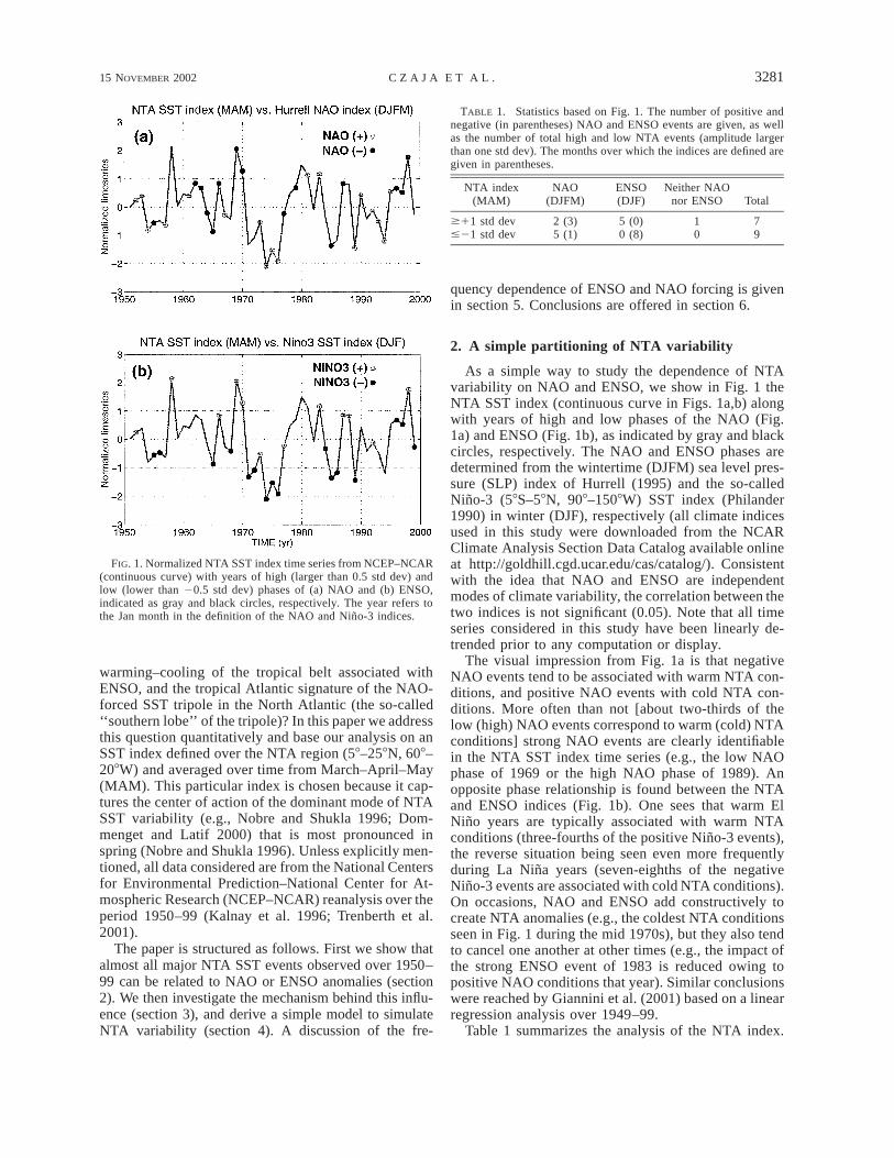
FIG. 1. Normalized NTA SST index time series from NCEP–NCAR(continuous curve) with years of high (larger than 0.5 std dev) andlow (lower than 20.5 std dev) phases of (a) NAO and (b) ENSO,indicated as gray and black circles, respectively. The year refers tothe Jan month in the definition of the NAO and Nino-3 indices.

TABLE 1. Statistics based on Fig. 1. The number of positive andnegative (in parentheses) NAO and ENSO events are given, as wellas the number of total high and low NTA events (amplitude largerthan one std dev). The months over which the indices are defined aregiven in parentheses.

NTA index(MAM)

NAO(DJFM)

ENSO(DJF)

Neither NAOnor ENSO Total

$11 std dev#21 std dev

2 (3)5 (1)

5 (0)0 (8)

10

79

warming–cooling of the tropical belt associated withENSO, and the tropical Atlantic signature of the NAO-forced SST tripole in the North Atlantic (the so-called‘‘southern lobe’’ of the tripole)? In this paper we addressthis question quantitatively and base our analysis on anSST index defined over the NTA region (58–258N, 608–208W) and averaged over time from March–April–May(MAM). This particular index is chosen because it cap-tures the center of action of the dominant mode of NTASST variability (e.g., Nobre and Shukla 1996; Dom-menget and Latif 2000) that is most pronounced inspring (Nobre and Shukla 1996). Unless explicitly men-tioned, all data considered are from the National Centersfor Environmental Prediction–National Center for At-mospheric Research (NCEP–NCAR) reanalysis over theperiod 1950–99 (Kalnay et al. 1996; Trenberth et al.2001).

The paper is structured as follows. First we show thatalmost all major NTA SST events observed over 1950–99 can be related to NAO or ENSO anomalies (section2). We then investigate the mechanism behind this influ-ence (section 3), and derive a simple model to simulateNTA variability (section 4). A discussion of the fre-

quency dependence of ENSO and NAO forcing is givenin section 5. Conclusions are offered in section 6.

2. A simple partitioning of NTA variability

As a simple way to study the dependence of NTAvariability on NAO and ENSO, we show in Fig. 1 theNTA SST index (continuous curve in Figs. 1a,b) alongwith years of high and low phases of the NAO (Fig.1a) and ENSO (Fig. 1b), as indicated by gray and blackcircles, respectively. The NAO and ENSO phases aredetermined from the wintertime (DJFM) sea level pres-sure (SLP) index of Hurrell (1995) and the so-calledNino-3 (58S–58N, 908–1508W) SST index (Philander1990) in winter (DJF), respectively (all climate indicesused in this study were downloaded from the NCARClimate Analysis Section Data Catalog available onlineat http://goldhill.cgd.ucar.edu/cas/catalog/). Consistentwith the idea that NAO and ENSO are independentmodes of climate variability, the correlation between thetwo indices is not significant (0.05). Note that all timeseries considered in this study have been linearly de-trended prior to any computation or display.

The visual impression from Fig. 1a is that negativeNAO events tend to be associated with warm NTA con-ditions, and positive NAO events with cold NTA con-ditions. More often than not [about two-thirds of thelow (high) NAO events correspond to warm (cold) NTAconditions] strong NAO events are clearly identifiablein the NTA SST index time series (e.g., the low NAOphase of 1969 or the high NAO phase of 1989). Anopposite phase relationship is found between the NTAand ENSO indices (Fig. 1b). One sees that warm ElNino years are typically associated with warm NTAconditions (three-fourths of the positive Nino-3 events),the reverse situation being seen even more frequentlyduring La Nina years (seven-eighths of the negativeNino-3 events are associated with cold NTA conditions).On occasions, NAO and ENSO add constructively tocreate NTA anomalies (e.g., the coldest NTA conditionsseen in Fig. 1 during the mid 1970s), but they also tendto cancel one another at other times (e.g., the impact ofthe strong ENSO event of 1983 is reduced owing topositive NAO conditions that year). Similar conclusionswere reached by Giannini et al. (2001) based on a linearregression analysis over 1949–99.

Table 1 summarizes the analysis of the NTA index.


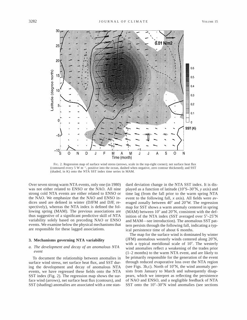
FIG. 2. Regression map of surface wind stress (arrows, scale in the top-right corner); net surface heat flux(contoured every 5 W m22, positive into the ocean, dashed when negative, zero contour thickened); and SST(shaded, in K) onto the NTA SST index time series in MAM.

Over seven strong warm NTA events, only one (in 1980)was not either related to ENSO or the NAO. All ninestrong cold NTA events are either related to ENSO orthe NAO. We emphasize that the NAO and ENSO in-dices used are defined in winter (DJFM and DJF, re-spectively), whereas the NTA index is defined the fol-lowing spring (MAM). The previous associations arethus suggestive of a significant predictive skill of NTAvariability solely based on preceding NAO or ENSOevents. We examine below the physical mechanisms thatare responsible for these lagged associations.

3. Mechanisms governing NTA variability

a. The development and decay of an anomalous NTAevent

To document the relationship between anomalies insurface wind stress, net surface heat flux, and SST dur-ing the development and decay of anomalous NTAevents, we have regressed these fields onto the NTASST index (Fig. 2). The regression map shows the sur-face wind (arrows), net surface heat flux (contours), andSST (shading) anomalies are associated with a one stan-

dard deviation change in the NTA SST index. It is dis-played as a function of latitude (108S–308N, y axis) andtime lag (from the fall prior to the warm spring NTAevent to the following fall, x axis). All fields were av-eraged zonally between 408 and 208W. The regressionmap for SST shows a warm anomaly centered in spring(MAM) between 108 and 208N, consistent with the def-inition of the NTA index (SST averaged over 58–258Nand MAM—see introduction). The anomalous SST pat-tern persists through the following fall, indicating a typ-ical persistence time of about 6 months.

The map for the surface wind is dominated by winter(JFM) anomalous westerly winds centered along 208N,with a typical meridional scale of 108. The westerlywind anomalies reflect a weakening of the trades prior(1–2 months) to the warm NTA event, and are likely tobe primarily responsible for the generation of the eventthrough reduced evaporative loss over the NTA region(see Figs. 3b,c). North of 108N, the wind anomaly per-sists from January to March and subsequently disap-pears, which we interpret as reflecting the persistenceof NAO and ENSO, and a negligible feedback of NTASST onto the 108–308N wind anomalies (see sections


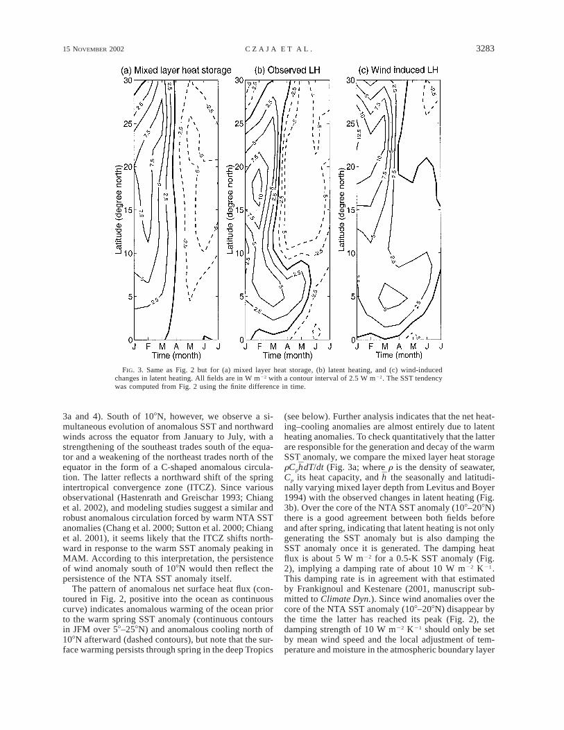
FIG. 3. Same as Fig. 2 but for (a) mixed layer heat storage, (b) latent heating, and (c) wind-inducedchanges in latent heating. All fields are in W m22 with a contour interval of 2.5 W m22. The SST tendencywas computed from Fig. 2 using the finite difference in time.

3a and 4). South of 108N, however, we observe a si-multaneous evolution of anomalous SST and northwardwinds across the equator from January to July, with astrengthening of the southeast trades south of the equa-tor and a weakening of the northeast trades north of theequator in the form of a C-shaped anomalous circula-tion. The latter reflects a northward shift of the springintertropical convergence zone (ITCZ). Since variousobservational (Hastenrath and Greischar 1993; Chianget al. 2002), and modeling studies suggest a similar androbust anomalous circulation forced by warm NTA SSTanomalies (Chang et al. 2000; Sutton et al. 2000; Chianget al. 2001), it seems likely that the ITCZ shifts north-ward in response to the warm SST anomaly peaking inMAM. According to this interpretation, the persistenceof wind anomaly south of 108N would then reflect thepersistence of the NTA SST anomaly itself.

The pattern of anomalous net surface heat flux (con-toured in Fig. 2, positive into the ocean as continuouscurve) indicates anomalous warming of the ocean priorto the warm spring SST anomaly (continuous contoursin JFM over 58–258N) and anomalous cooling north of108N afterward (dashed contours), but note that the sur-face warming persists through spring in the deep Tropics

(see below). Further analysis indicates that the net heat-ing–cooling anomalies are almost entirely due to latentheating anomalies. To check quantitatively that the latterare responsible for the generation and decay of the warmSST anomaly, we compare the mixed layer heat storagerCp dT/dt (Fig. 3a; where r is the density of seawater,hCp its heat capacity, and the seasonally and latitudi-hnally varying mixed layer depth from Levitus and Boyer1994) with the observed changes in latent heating (Fig.3b). Over the core of the NTA SST anomaly (108–208N)there is a good agreement between both fields beforeand after spring, indicating that latent heating is not onlygenerating the SST anomaly but is also damping theSST anomaly once it is generated. The damping heatflux is about 5 W m22 for a 0.5-K SST anomaly (Fig.2), implying a damping rate of about 10 W m22 K21.This damping rate is in agreement with that estimatedby Frankignoul and Kestenare (2001, manuscript sub-mitted to Climate Dyn.). Since wind anomalies over thecore of the NTA SST anomaly (108–208N) disappear bythe time the latter has reached its peak (Fig. 2), thedamping strength of 10 W m22 K21 should only be setby mean wind speed and the local adjustment of tem-perature and moisture in the atmospheric boundary layer


to the NTA SST anomaly (Frankignoul et al. 1998).Note that for a typical mixed layer depth of 40 m, 10W m22 K21 amounts to a persistence time of 6 months,consistent with that suggested in Fig. 2.

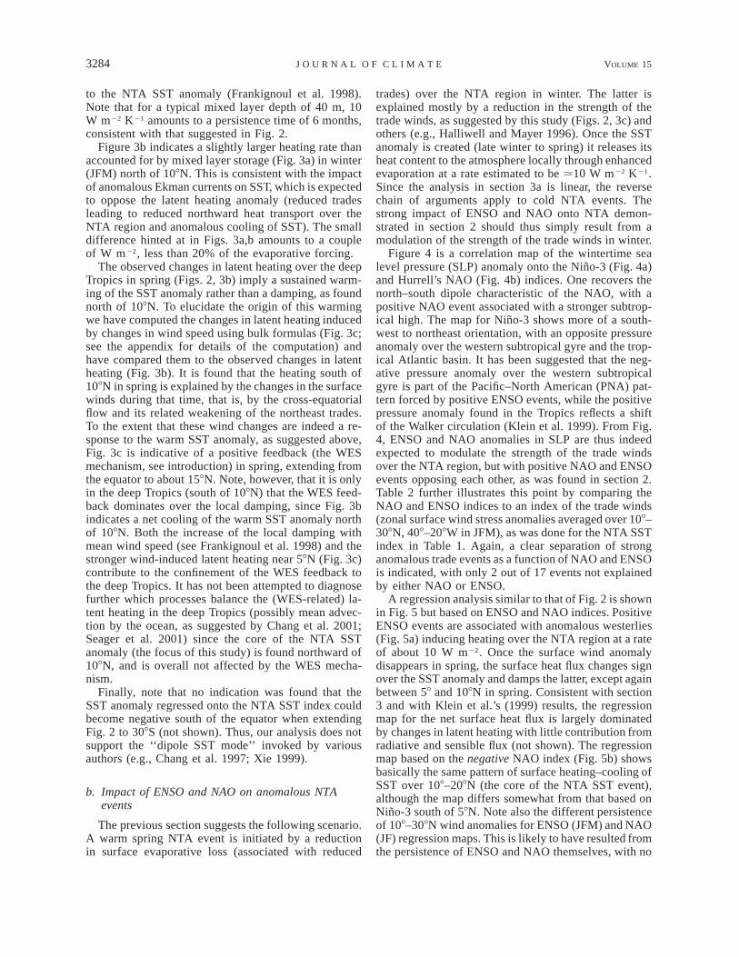
Figure 3b indicates a slightly larger heating rate thanaccounted for by mixed layer storage (Fig. 3a) in winter(JFM) north of 108N. This is consistent with the impactof anomalous Ekman currents on SST, which is expectedto oppose the latent heating anomaly (reduced tradesleading to reduced northward heat transport over theNTA region and anomalous cooling of SST). The smalldifference hinted at in Figs. 3a,b amounts to a coupleof W m22, less than 20% of the evaporative forcing.

The observed changes in latent heating over the deepTropics in spring (Figs. 2, 3b) imply a sustained warm-ing of the SST anomaly rather than a damping, as foundnorth of 108N. To elucidate the origin of this warmingwe have computed the changes in latent heating inducedby changes in wind speed using bulk formulas (Fig. 3c;see the appendix for details of the computation) andhave compared them to the observed changes in latentheating (Fig. 3b). It is found that the heating south of108N in spring is explained by the changes in the surfacewinds during that time, that is, by the cross-equatorialflow and its related weakening of the northeast trades.To the extent that these wind changes are indeed a re-sponse to the warm SST anomaly, as suggested above,Fig. 3c is indicative of a positive feedback (the WESmechanism, see introduction) in spring, extending fromthe equator to about 158N. Note, however, that it is onlyin the deep Tropics (south of 108N) that the WES feed-back dominates over the local damping, since Fig. 3bindicates a net cooling of the warm SST anomaly northof 108N. Both the increase of the local damping withmean wind speed (see Frankignoul et al. 1998) and thestronger wind-induced latent heating near 58N (Fig. 3c)contribute to the confinement of the WES feedback tothe deep Tropics. It has not been attempted to diagnosefurther which processes balance the (WES-related) la-tent heating in the deep Tropics (possibly mean advec-tion by the ocean, as suggested by Chang et al. 2001;Seager et al. 2001) since the core of the NTA SSTanomaly (the focus of this study) is found northward of108N, and is overall not affected by the WES mecha-nism.

Finally, note that no indication was found that theSST anomaly regressed onto the NTA SST index couldbecome negative south of the equator when extendingFig. 2 to 308S (not shown). Thus, our analysis does notsupport the ‘‘dipole SST mode’’ invoked by variousauthors (e.g., Chang et al. 1997; Xie 1999).

b. Impact of ENSO and NAO on anomalous NTAevents

The previous section suggests the following scenario.A warm spring NTA event is initiated by a reductionin surface evaporative loss (associated with reduced

trades) over the NTA region in winter. The latter isexplained mostly by a reduction in the strength of thetrade winds, as suggested by this study (Figs. 2, 3c) andothers (e.g., Halliwell and Mayer 1996). Once the SSTanomaly is created (late winter to spring) it releases itsheat content to the atmosphere locally through enhancedevaporation at a rate estimated to be .10 W m22 K21.Since the analysis in section 3a is linear, the reversechain of arguments apply to cold NTA events. Thestrong impact of ENSO and NAO onto NTA demon-strated in section 2 should thus simply result from amodulation of the strength of the trade winds in winter.

Figure 4 is a correlation map of the wintertime sealevel pressure (SLP) anomaly onto the Nino-3 (Fig. 4a)and Hurrell’s NAO (Fig. 4b) indices. One recovers thenorth–south dipole characteristic of the NAO, with apositive NAO event associated with a stronger subtrop-ical high. The map for Nino-3 shows more of a south-west to northeast orientation, with an opposite pressureanomaly over the western subtropical gyre and the trop-ical Atlantic basin. It has been suggested that the neg-ative pressure anomaly over the western subtropicalgyre is part of the Pacific–North American (PNA) pat-tern forced by positive ENSO events, while the positivepressure anomaly found in the Tropics reflects a shiftof the Walker circulation (Klein et al. 1999). From Fig.4, ENSO and NAO anomalies in SLP are thus indeedexpected to modulate the strength of the trade windsover the NTA region, but with positive NAO and ENSOevents opposing each other, as was found in section 2.Table 2 further illustrates this point by comparing theNAO and ENSO indices to an index of the trade winds(zonal surface wind stress anomalies averaged over 108–308N, 408–208W in JFM), as was done for the NTA SSTindex in Table 1. Again, a clear separation of stronganomalous trade events as a function of NAO and ENSOis indicated, with only 2 out of 17 events not explainedby either NAO or ENSO.

A regression analysis similar to that of Fig. 2 is shownin Fig. 5 but based on ENSO and NAO indices. PositiveENSO events are associated with anomalous westerlies(Fig. 5a) inducing heating over the NTA region at a rateof about 10 W m22. Once the surface wind anomalydisappears in spring, the surface heat flux changes signover the SST anomaly and damps the latter, except againbetween 58 and 108N in spring. Consistent with section3 and with Klein et al.’s (1999) results, the regressionmap for the net surface heat flux is largely dominatedby changes in latent heating with little contribution fromradiative and sensible flux (not shown). The regressionmap based on the negative NAO index (Fig. 5b) showsbasically the same pattern of surface heating–cooling ofSST over 108–208N (the core of the NTA SST event),although the map differs somewhat from that based onNino-3 south of 58N. Note also the different persistenceof 108–308N wind anomalies for ENSO (JFM) and NAO(JF) regression maps. This is likely to have resulted fromthe persistence of ENSO and NAO themselves, with no


FIG. 4. Correlation map of wintertime (JFM) SLP anomaly and (a) DJF Nino-3 SST index, and (b) DJFMNAO index of Hurrell. Correlations are contoured every 0.2, dashed when negative. The zero contour isomitted. A correlation of 0.3 is significant at the 95% level, assuming independent samples. The NAO andENSO indices are the same as those used in Fig. 1.

TABLE 2. Same as Table 1 but for an index of the trade winds(see text for a definition). A positive value of the trade wind indexindicates anomalous westerly wind, i.e., reduced trade winds.

Trade windsindex (JFM)

NAO(DJFM)

ENSO(DJF)

Neither NAOnor ENSO Total

$11 std dev#21 std dev

0 (7)5 (0)

6 (1)0 (4)

11

98

additional memory added to the wind anomaly by thelocal interaction with the NTA SST. This latter point—negligible feedback of NTA SST anomaly on the 108–308N surface wind—is further discussed in section 4.

In summary, a similar mechanism is responsible forthe forcing of NTA variability by both ENSO and NAO.It consists in a modulation of latent heating throughchanges in trade wind speeds and a subsequent localdamping through air–sea interactions. The fact that al-most all strong NTA SST and trade winds events canbe related to either NAO or ENSO (Tables 1 and 2)suggests that a simple model driven by observed NAOand ENSO wind anomalies should capture NTA vari-ability. This is studied in the next section.

4. A simple model for NTA variability

Let us assume, motivated by the previous section, thatSST anomalies over the NTA region are essentially driv-en by changes in latent heating. That is,

dTrC h 5 F , (1)p 0 latdt

where h0 is an annual mean mixed layer depth (h0 540 m is found when averaging over time and latitude),hFlat the latent heating (positive when warming theocean), and T the SST, all fields averaged over the NTAregion (58–258N, 608–208W).

As a simple index of wind anomalies associated withNAO and ENSO, Fig. 4 suggests that we average SLPanomalies north of the NTA region, say 208–408N, 708–108W.1 Positive anomalies of that index (denoted bySTH for subtropical high) reflect a strengthening of thetrades and yield enhanced evaporative loss over theNTA region (Flat , 0). Since anomalous heating is alsoaffected by the SST anomaly, once the latter is gener-ated, we write

F 5 2a STH 2 gT,lat (2)

where a (positive, in W m22 mb21) scales a change inthe strength of the subtropical high into a change inlatent heating, and g (in W m22 K21) measures thesensitivity of Flat to SST. Combining (1) and (2), weobtain

dTrC h 5 2aSTH 2 gT. (3)p 0 dt

1 The choice of an SLP index rather than wind stress will allowus to use the long record of reconstructed SLP anomalies of Kaplanet al. 2000 (see below).


FIG. 5. Same as Fig. 2 but regressed onto (a) Nino-3 SST index, and (b) negative NAO index.

FIG. 6. Cross-correlation function between the monthly NTA SSTand STH indices (see text for a definition). STH leads at positivelags (in months). The dashed gray lines indicate an approximate 95%confidence level, taking into account the month-to-month persistenceof the STH index.

The latter model is probably the simplest proposed sofar for NTA variability. It is close to that of Frankignouland Hasselman (1977) for extratropical SST anomalies.Note, however, that the forcing (the STH index) isslightly red, rather than white as in Frankignoul andHasselman (1977), because of the influence of NAOand ENSO on the subtropical high. It is assumed thatthe strength of the subtropical high is not affected bythe NTA SST anomaly, so that the only feedback in-cluded in the model is the local damping effect of latentheating. This assumption is supported by an analysis ofthe correlation between NTA SST and STH (Fig. 6).The correlation function is strongly asymmetric withtemporal lag, having a minimum when SST lags by onemonth (strong STH drives cold SST), and not beingsignificant when SST leads STH. This is a known sig-nature of one-way forcing of the ocean by the atmo-sphere (e.g., Frankignoul 1985).2 Note that very similarresults are obtained when the trade wind index of Table2 rather than STH is used when computing the cross-correlation function (not shown).

The model (3) has two parameters, a and g. As de-tailed in the appendix, the scaling factor a can be rough-

2 Note that the marginal correlation observed in Fig. 6 when SSTleads STH by one month is likely to reflect the month-to-monthpersistence of the subtropical high, rather than a feedback of the NTASST anomaly onto the subtropical high (e.g., Frankignoul et al. 1998).


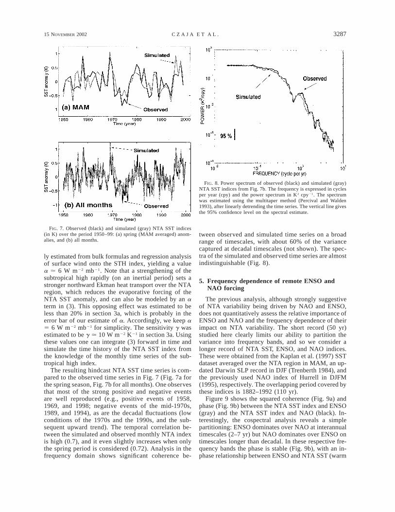
FIG. 7. Observed (black) and simulated (gray) NTA SST indices(in K) over the period 1950–99: (a) spring (MAM averaged) anom-alies, and (b) all months.

FIG. 8. Power spectrum of observed (black) and simulated (gray)NTA SST indices from Fig. 7b. The frequency is expressed in cyclesper year (cpy) and the power spectrum in K2 cpy21. The spectrumwas estimated using the multitaper method (Percival and Walden1993), after linearly detrending the time series. The vertical line givesthe 95% confidence level on the spectral estimate.

ly estimated from bulk formulas and regression analysisof surface wind onto the STH index, yielding a valuea . 6 W m22 mb21. Note that a strengthening of thesubtropical high rapidly (on an inertial period) sets astronger northward Ekman heat transport over the NTAregion, which reduces the evaporative forcing of theNTA SST anomaly, and can also be modeled by an aterm in (3). This opposing effect was estimated to beless than 20% in section 3a, which is probably in theerror bar of our estimate of a. Accordingly, we keep a5 6 W m22 mb21 for simplicity. The sensitivity g wasestimated to be g . 10 W m22 K21 in section 3a. Usingthese values one can integrate (3) forward in time andsimulate the time history of the NTA SST index fromthe knowledge of the monthly time series of the sub-tropical high index.

The resulting hindcast NTA SST time series is com-pared to the observed time series in Fig. 7 (Fig. 7a forthe spring season, Fig. 7b for all months). One observesthat most of the strong positive and negative eventsare well reproduced (e.g., positive events of 1958,1969, and 1998; negative events of the mid-1970s,1989, and 1994), as are the decadal fluctuations (lowconditions of the 1970s and the 1990s, and the sub-sequent upward trend). The temporal correlation be-tween the simulated and observed monthly NTA indexis high (0.7), and it even slightly increases when onlythe spring period is considered (0.72). Analysis in thefrequency domain shows significant coherence be-

tween observed and simulated time series on a broadrange of timescales, with about 60% of the variancecaptured at decadal timescales (not shown). The spec-tra of the simulated and observed time series are almostindistinguishable (Fig. 8).

5. Frequency dependence of remote ENSO andNAO forcing

The previous analysis, although strongly suggestiveof NTA variability being driven by NAO and ENSO,does not quantitatively assess the relative importance ofENSO and NAO and the frequency dependence of theirimpact on NTA variability. The short record (50 yr)studied here clearly limits our ability to partition thevariance into frequency bands, and so we consider alonger record of NTA SST, ENSO, and NAO indices.These were obtained from the Kaplan et al. (1997) SSTdataset averaged over the NTA region in MAM, an up-dated Darwin SLP record in DJF (Trenberth 1984), andthe previously used NAO index of Hurrell in DJFM(1995), respectively. The overlapping period covered bythese indices is 1882–1992 (110 yr).

Figure 9 shows the squared coherence (Fig. 9a) andphase (Fig. 9b) between the NTA SST index and ENSO(gray) and the NTA SST index and NAO (black). In-terestingly, the cospectral analysis reveals a simplepartitioning: ENSO dominates over NAO at interannualtimescales (2–7 yr) but NAO dominates over ENSO ontimescales longer than decadal. In these respective fre-quency bands the phase is stable (Fig. 9b), with an in-phase relationship between ENSO and NTA SST (warm


FIG. 9. Cospectral analysis of NTA SST and ENSO (gray), andNTA SST and NAO (black) indices. (a) Squared coherence (the hor-izontal dashed line gives an approximate 95% confidence level), and(b) phase (in degrees). The cospectra were estimated using a Daniellwindow (averaged over six frequency bins).

FIG. 10. Time series of simulated (gray) and observed (black) NTASST in MAM (in K). Dashed lines indicate 10-yr running mean.

ENSO events covary with warm NTA SST events) butout-of-phase relationship (61808) between NAO andNTA SST (positive NAO events covary with cold NTASST events), in agreement with previous sections. FromFig. 9a, typically 70% of the NTA SST variance atinterannual timescales can be attributed to ENSO. NAOis seen to account for 50% of the low-frequency (decadaland interdecadal timescales) fluctuations of the NTASST index.

If the stronger coherence found with ENSO at time-scales of 2–7 years can be expected from the broadbandpeak displayed by the Nino-3 index in that band, thefrequency dependence of the coherence between NTASST and NAO is more intriguing because Hurrell’s NAOindex is only weakly red (Wunsch 1999). An interestingpossibility could be that the dominance of NAO overENSO at long timescales might result from changes inthe North Atlantic meridional overturning circulation(MOC) in addition to the evaporative forcing encap-sulated in (1). Indeed, both NAO and MOC have beensuggested to covary at interdecadal timescales, withlarge related changes in ocean heat transport at 258N(e.g., Hakkinen 1999; Eden and Jung 2001), whichcould impact NTA SST variability. To clarify the rel-evance of the model (3) at these long timescales wehave integrated (3) forward in time using a long timeseries of the STH index from Kaplan et al.’s (2000) SLPdata (1856–1992), and the same a and g as in section4. In the resulting spring (MAM), the NTA SST indexis compared to that from the Kaplan et al.’s (1997) SSTdata in Fig. 10, with a 10-yr running mean indicated asdashed lines. Again, one observes a good agreement

between simulated (gray) and observed (black) time se-ries at interannual timescales (the correlation of the rawtime series is 0.62). However, even better agreement isfound for the low-pass time series (the negative SSTtendency of 1880–1910, the positive tendency of 1920–60, and the subsequent negative tendency). Overall, Fig.10 strongly suggests that the model (3) is relevant atdecadal and longer timescales, and that geostrophicocean dynamics is of secondary importance even atthese long timescales in the hindcast of NTA SST var-iability. The weakness of mean SST gradients over 58–258N might limit the impact of changes in ocean cir-culation on the oceanic mixed layer heat budget at theselatitudes, and possibly explain the good simulation ofthe interdecadal changes in Fig. 10, but a complete ex-planation requires further modeling studies. We notethat, on the long term, ocean heat transport divergence–convergence is also not crucial over the NTA region,since net radiation and evaporation approximately bal-ance each other when annually and meridionally aver-aged over the latitude band 58–258N (not shown).

6. Conclusions

Almost all strong anomalies in the north tropical At-lantic (NTA) SST observed from 1950 to the presentcan be accounted for by prior ENSO or NAO events.The NAO and ENSO influence is felt through the semi-permanent subtropical high pressure system and the re-lated trade winds, whose intensity modulates the latentheating at the ocean surface. Once generated, a warmNTA SST anomaly releases its energy to the atmospherethrough enhanced evaporation at a rate of .10 W m22

K21. This local process sets the persistence of the anom-aly (about 6 months); the positive (WES) feedback hint-ed at in our study occurs too far to the south (08–108N)to significantly impact the evolution of the NTA SSTanomaly. A simple model combining these elements,Eq. (3), is successful in simulating NTA variability ontimescales ranging from interannual to interdecadal.

On the evidence of the observations and models an-alyzed here, there does not appear to be significant in-trinsic north tropical Atlantic variability. Local geo-strophic ocean dynamics and large-scale unstable air–


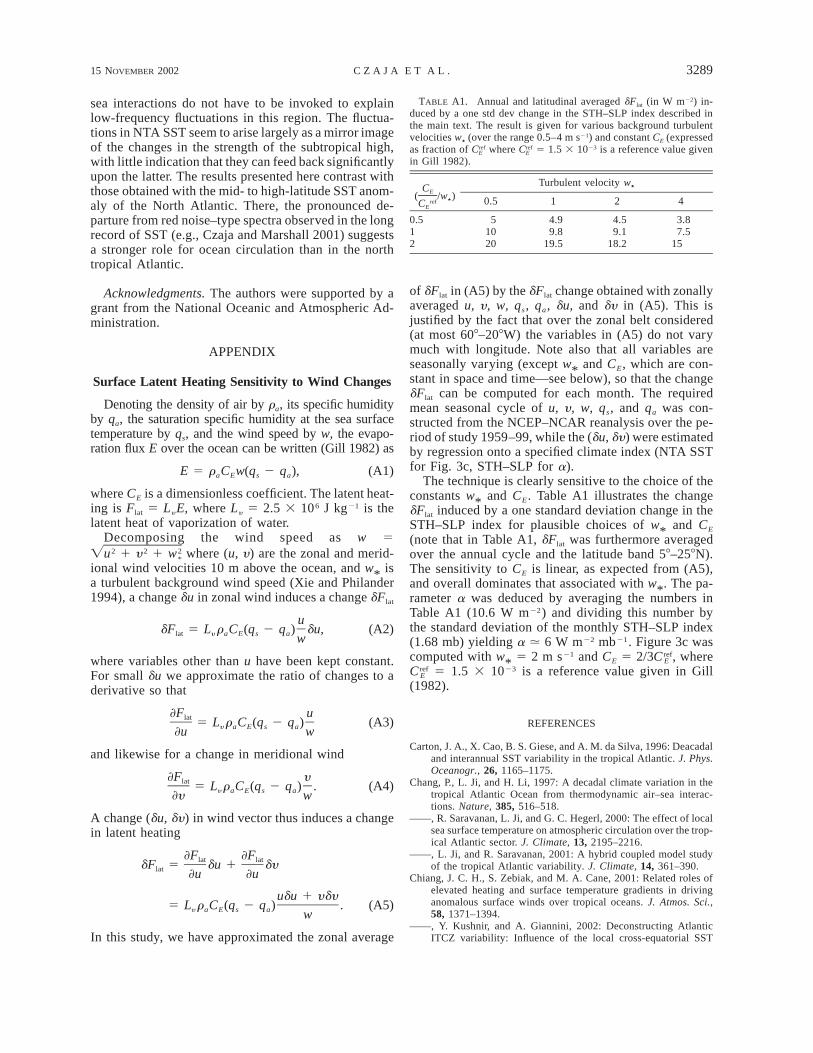
TABLE A1. Annual and latitudinal averaged dFlat (in W m22) in-duced by a one std dev change in the STH–SLP index described inthe main text. The result is given for various background turbulentvelocities w, (over the range 0.5–4 m s21) and constant CE (expressedas fraction of C where C 5 1.5 3 1023 is a reference value givenref ref

E E

in Gill 1982).

( /w,)CE

refCE

Turbulent velocity w,

0.5 1 2 4

0.512

51020

4.99.8

19.5

4.59.1

18.2

3.87.5

15

sea interactions do not have to be invoked to explainlow-frequency fluctuations in this region. The fluctua-tions in NTA SST seem to arise largely as a mirror imageof the changes in the strength of the subtropical high,with little indication that they can feed back significantlyupon the latter. The results presented here contrast withthose obtained with the mid- to high-latitude SST anom-aly of the North Atlantic. There, the pronounced de-parture from red noise–type spectra observed in the longrecord of SST (e.g., Czaja and Marshall 2001) suggestsa stronger role for ocean circulation than in the northtropical Atlantic.

Acknowledgments. The authors were supported by agrant from the National Oceanic and Atmospheric Ad-ministration.

APPENDIX

Surface Latent Heating Sensitivity to Wind Changes

Denoting the density of air by ra, its specific humidityby qa, the saturation specific humidity at the sea surfacetemperature by qs, and the wind speed by w, the evapo-ration flux E over the ocean can be written (Gill 1982) as

E 5 r C w(q 2 q ),a E s a (A1)

where CE is a dimensionless coefficient. The latent heat-ing is Flat 5 Ly E, where Ly 5 2.5 3 106 J kg21 is thelatent heat of vaporization of water.

Decomposing the wind speed as w 5where (u, y) are the zonal and merid-2 2 2Ïu 1 y 1 w*

ional wind velocities 10 m above the ocean, and w* isa turbulent background wind speed (Xie and Philander1994), a change du in zonal wind induces a change dFlat

udF 5 L r C (q 2 q ) du, (A2)lat y a E s a w

where variables other than u have been kept constant.For small du we approximate the ratio of changes to aderivative so that

]F ulat 5 L r C (q 2 q ) (A3)y a E s a]u w

and likewise for a change in meridional wind

]F ylat 5 L r C (q 2 q ) . (A4)y a E s a]y w

A change (du, dy) in wind vector thus induces a changein latent heating

]F ]Flat latdF 5 du 1 dylat ]u ]u

udu 1 ydy5 L r C (q 2 q ) . (A5)y a E s a w

In this study, we have approximated the zonal average

of dFlat in (A5) by the dFlat change obtained with zonallyaveraged u, y, w, qs, qa, du, and dy in (A5). This isjustified by the fact that over the zonal belt considered(at most 608–208W) the variables in (A5) do not varymuch with longitude. Note also that all variables areseasonally varying (except w* and CE, which are con-stant in space and time—see below), so that the changedFlat can be computed for each month. The requiredmean seasonal cycle of u, y, w, qs, and qa was con-structed from the NCEP–NCAR reanalysis over the pe-riod of study 1959–99, while the (du, dy) were estimatedby regression onto a specified climate index (NTA SSTfor Fig. 3c, STH–SLP for a).

The technique is clearly sensitive to the choice of theconstants w* and CE. Table A1 illustrates the changedFlat induced by a one standard deviation change in theSTH–SLP index for plausible choices of w* and CE

(note that in Table A1, dFlat was furthermore averagedover the annual cycle and the latitude band 58–258N).The sensitivity to CE is linear, as expected from (A5),and overall dominates that associated with w*. The pa-rameter a was deduced by averaging the numbers inTable A1 (10.6 W m22) and dividing this number bythe standard deviation of the monthly STH–SLP index(1.68 mb) yielding a . 6 W m22 mb21. Figure 3c wascomputed with w* 5 2 m s21 and CE 5 2/3 , whererefC E

5 1.5 3 1023 is a reference value given in GillrefC E

(1982).

REFERENCES

Carton, J. A., X. Cao, B. S. Giese, and A. M. da Silva, 1996: Deacadaland interannual SST variability in the tropical Atlantic. J. Phys.Oceanogr., 26, 1165–1175.

Chang, P., L. Ji, and H. Li, 1997: A decadal climate variation in thetropical Atlantic Ocean from thermodynamic air–sea interac-tions. Nature, 385, 516–518.

——, R. Saravanan, L. Ji, and G. C. Hegerl, 2000: The effect of localsea surface temperature on atmospheric circulation over the trop-ical Atlantic sector. J. Climate, 13, 2195–2216.

——, L. Ji, and R. Saravanan, 2001: A hybrid coupled model studyof the tropical Atlantic variability. J. Climate, 14, 361–390.

Chiang, J. C. H., S. Zebiak, and M. A. Cane, 2001: Related roles ofelevated heating and surface temperature gradients in drivinganomalous surface winds over tropical oceans. J. Atmos. Sci.,58, 1371–1394.

——, Y. Kushnir, and A. Giannini, 2002: Deconstructing AtlanticITCZ variability: Influence of the local cross-equatorial SST


gradient, and remote forcing from the eastern equatorial Pacific.J. Geophys. Res., 107 (D1), 1–19.

Covey, D., and S. Hastenrath, 1978: The Pacific El Nino phenomenonand the Atlantic circulation. Mon. Wea. Rev., 106, 1280–1287.

Curtis, S., and S. Hastenrath, 1995: Forcing of anomalous sea surfacetemperature evolution in the tropical Atlantic during Pacificwarm events. J. Geophys. Res., 100 (C8), 15 835–15 847.

Czaja, A., and J. Marshall, 2001: Observations of atmosphere–oceancoupling in the North Atlantic. Quart. J. Roy. Meteor. Soc., 127,1893–1916.

Dommenget, D., and M. Latif, 2000: Interannual to decadal variabilityin the tropical Atlantic. J. Climate, 13, 777–792.

Eden, C., and T. Jung, 2001: North Atlantic interdecadal variability:Oceanic response to the North Atlantic Oscillation (1865–1997).J. Climate, 14, 676–691.

Enfield, D. B., and D. A. Mayer, 1997: Tropical Atlantic sea surfacetemperature variability and its relation to El Nino–Southern Os-cillation. J. Geophys. Res., 102, 929–945.

Frankignoul, C., 1985: Sea surface temperature anomalies, planetarywaves and air–sea feedbacks in the middle latitude. Rev. Geo-phys., 23, 357–390.

——, and K. Hasselman, 1977: Stochastic climate models. Part II:Application to sea-surface temperature variability and thermo-cline variability. Tellus, 29, 289–305.

——, A. Czaja, and B. L’Heveder, 1998: Air–sea feedback in theNorth Atlantic and surface boundary conditions for ocean mod-els. J. Climate, 11, 2310–2324.

Giannini, A., M. A. Cane, and Y. Kushnir, 2001: Interdecadal changesin the ENSO teleconnection to the Caribbean region and theNorth Atlantic Oscillation. J. Climate, 14, 2867–2879.

Gill, A. E., 1982: Atmosphere–Ocean Dynamics. International Geo-physical Series, Vol. 30, Academic Press, 662 pp.

Grotzner, A., M. Latif, and T. P. Barnett, 1998: A decadal climatecycle in the North Atlantic Ocean as simulated by the ECHOcoupled GCM. J. Climate, 11, 831–847.

Hakkinen, S., 1999: Variability of the simulated meridional heat trans-port in the North Atlantic for the period 1951–1993. J. Geophys.Res., 104 (C5), 10 991–11 007.

Halliwell, G. R., 1998: Simulation of North Atlantic decadal/multi-decadal winter SST anomalies driven by basin-scale atmosphericcirculation anomalies. J. Phys. Oceanogr., 28, 5–21.

——, and D. A. Mayer, 1996: Frequency response properties of forcedclimatic SST anomaly variability in the North Atlantic. J. Cli-mate, 9, 3575–3587.

Hastenrath, S., and L. Greischar, 1993: Circulation mechanisms re-lated to Northeast Brazil rainfall anomalies. J. Geophys. Res.,98 (D3), 5093–5102.

Hurrell, J., 1995: Decadal trends in the North Atlantic Oscillation:Regional temperature and precipitation. Science, 269, 676–679.

Kalnay, E., and Coauthors, 1996: The NCEP/NCAR 40-Year Re-analysis Project. Bull. Amer. Meteor. Soc., 77, 437–471.

Kaplan, A., Y. Kushnir, M. Cane, and B. Blumenthal, 1997: Reducedspace optimal analysis for historical datasets: 136 years of At-lantic sea surface temperatures. J. Geophys. Res., 102, 27 835–27 860.

——, ——, and ——, 2000: Reduced space optimal interpolation ofhistorical marine sea level pressure: 1854–1992. J. Climate, 13,2987–3002.

Klein, S. A., B. J. Soden, and N.-C. Lau, 1999: Remote sea surfacevariations during ENSO: Evidence for a tropical atmosphericbridge. J. Climate, 12, 917–932.

Levitus, S., and T. Boyer, 1994: Temperature. Vol 4, World OceanAtlas 1994, NOAA Atlas NESDIS 4, 117 pp.

Marshall, J., and Coauthors, 2001: Atlantic climate variability. Int.J. Climatol., 21, 1863–1898.

Nobre, P., and J. Shukla, 1996: Variations in sea surface temperature,wind stress, and rainfall over the tropical Atlantic and SouthAmerica. J. Climate, 9, 2464–2479.

Percival, D. B., and T. A. Walden, 1993: Spectral Analysis for Phys-ical Applications: Multitaper and Conventionnal UnivariateTechniques. Cambridge University Press, 583 pp.

Philander, S. G. H., 1990: El Nino, La Nina, and the Southern Os-cillation. International Geophysics Series, Vol. 46, AcademicPress, 293 pp.

Saravanan, R., and P. Chang, 2000: Interaction between tropical At-lantic variability and El Nino–Southern Oscillation. J. Climate,13, 2177–2194.

Seager, R., Y. Kushnir, P. Chang, N. Naik, J. Miller, and W. Hazeleger,2001: Looking for the role of ocean in tropical Atlantic decadalclimate variability. J. Climate, 14, 638–655.

Sutton, R. T., S. P. Jewson, and D. P. Rowell, 2000: The elements ofclimate variability in the tropical Atlantic region. J. Climate, 13,3261–3284.

Trenberth, K. E., 1984: Signal versus noise in the Southern Oscil-lation. Mon. Wea. Rev., 112, 326–332.

——, D. P. Stepaniak, and J. W. Hurrell, 2001: Quality of reanalysesin the Tropics. J. Climate, 14, 1499–1510.

Wunsch, C., 1999: The interpretation of short climate records, withcomments on the North Atlantic Oscillation and Southern Os-cillations. Bull. Amer. Meteor. Soc., 80, 245–255.

Xie, S. P., 1999: A dynamic ocean–atmosphere model of the tropicalAtlantic decadal variability. J. Climate, 12, 64–70.

——, and S. G. H. Philander, 1994: A coupled ocean–atmospheremodel of relevance to the ITCZ in the eastern Pacific. Tellus,46A, 340–350.

a diagnostic study of the role of remote forcing in

Documents