a demonstration using low-kt fatigue specimens of a … · the trailing edge flap lug of the f/a-18...
TRANSCRIPT
UNCLASSIFIED
A Demonstration using Low-kt Fatigue Specimens of a Method for Predicting the Fatigue Behaviour of
Corroded Aircraft Components
Bruce R. Crawford, Chris Loader, Timothy J. Harrison and Qianchu Liu
Air Vehicles Division Defence Science and Technology Organisation
DSTO-RR-0390
ABSTRACT
Corrosion is well known to reduce the structural integrity of aluminium alloy aircraft components. In addition, it can cause early fatigue failures in components in which fatigue is not considered to be a life limiting factor. This is because corrosion damage, such as corrosion pits, is up to 100 times the size of the inclusions intrinsic in most aerospace aluminium alloys. The trailing edge flap lug of the F/A-18 Hornet aircraft is an example of an unexpected failure due to corrosion damage. In this report a Monte Carlo model is developed to simulate this phenomenon. This model predicts the fatigue lives of corroded and uncorroded specimens of the aluminium alloy 7010-T7651. It does this using high-quality fatigue crack growth data for this alloy from a previous research project (SICAS) combined with probability density functions for size of the corrosion pits and inclusions in this alloy. The distribution of the predicted fatigue lives is an excellent match for that observed in the SICAS project. The model was then extended to predict the location of fatigue failures. It showed that with good laboratory data the model could very accurately predict the location and life of pitting-induced fatigue failures.
RELEASE LIMITATION Approved for public release
UNCLASSIFIED
UNCLASSIFIED
Published by Air Vehicles Division DSTO Defence Science and Technology Organisation 506 Lorimer St Fishermans Bend, Victoria 3207 Australia Telephone: (03) 9626 7000 Fax: (03) 9626 7999 © Commonwealth of Australia 2013 AR-015-575 April 2013 APPROVED FOR PUBLIC RELEASE
UNCLASSIFIED
UNCLASSIFIED
UNCLASSIFIED
A Demonstration using Low-kt Fatigue Specimens of a Method for Predicting the Fatigue Behaviour of
Corroded Aircraft Components
Executive Summary The unexpected failure due to fatigue of the trailing edge flap (TEF) lugs of an Royal Australian Air Force (RAAF) F/A-18 in 1993 showed that, if neglected, corrosion can severely reduce aircraft structural integrity. It has become apparent, since at least the 1980s, that corrosion is a major cost in maintaining fleets of aircraft. The Defence Science and Technology Organisation (DSTO) has accordingly conducted a great deal of research into this issue. This research has principally concentrated on how corrosion reduces the fatigue endurance of aircraft components. The F/A-18 TEF lug failure showed that corrosion can create new modes of structural failure. Specifically, the lug that failed had been designed to have an effectively infinite life. There was therefore no expectation that it was a fatigue critical part. Despite this the presence of corrosion pits in the lug made it fatigue critical and its failure due to fatigue was unexpected and nearly catastrophic. The research described in this report is intended to address this issue. The approach taken was to develop a Monte Carlo model of the fatigue life of corroded specimens of aluminium alloy 7010-T7651. The model simulates both the alloy’s metallurgical inclusions and corrosion pits using extreme value statistical distributions. The inclusions are spread randomly across the specimen’s surface while the corrosion pits are contained in corrosion strikes of set size and location. The model was then used to predict the fatigue life distribution of corroded and uncorroded 7010-T7651. The model’s fatigue life predictions were found to be very accurate when compared to the results of an earlier research program conducted at DSTO. The model’s prediction of failure locations were compared to experimental results from a small trial conducted as part of the current work and were again found to be accurate. It is concluded that the model developed here should be expanded to deal with real aircraft components and more complex corrosion conditions. It should also be combined with models for corrosion nucleation and growth to create an end-to-end corrosion prediction model for the RAAF’s fleet of aircraft.

UNCLASSIFIED
UNCLASSIFIED
This page is intentionally blank

UNCLASSIFIED
UNCLASSIFIED
Authors
Dr. Bruce R. Crawford Air Vehicles Division Dr. Bruce Crawford, Senior Research Scientist, graduated from Monash University in 1991 with a Bachelor of Engineering in Materials Engineering with first class honours. He subsequently completed a Doctor of Philosophy at the University of Queensland in the field of fatigue of metal matrix composite materials. Bruce then lectured on materials science and engineering for four years at Deakin University in the School of Engineering and Technology before joining DSTO in 1999. Since joining DSTO Bruce has worked on the development of deterministic and probabilistic models of corrosion-fatigue and structural integrity management for aerospace aluminium alloys. In the past six years, he has managed the certification of Retrogression and Re-ageing, a technology with the potential to significantly reduce the incidence of exfoliation corrosion and stress corrosion cracking in the 7075 T6 components of the RAAF C-130 Hercules.
____________________ ________________________________________________
Chris Loader Air Vehicles Division Christopher Loader, Research Scientist, graduated from Monash University in 1998 with Bachelors degrees in Science and Engineering. Since arriving at DSTO in 1998, he has worked on several programs aimed at better understanding corrosion-initiated fatigue in a variety of aerospace aluminium and steel alloys. Chris is currently assessing several novel technologies for use in future and current Australian Defence Force aircraft. For the past year he has been managing the certification of Retrogression and Re-ageing for use on the RAAF C-130 Hercules.
____________________ ________________________________________________
UNCLASSIFIED
UNCLASSIFIED
Timothy J. Harrison RMIT University Timothy J. Harrison is currently a postgraduate student in the School of Aerospace, Mechanical and Manufacturing Engineering at RMIT University. His PhD studies are concerned with modelling the effect of intergranular corrosion on the structural integrity and fatigue life of the aluminium alloy 7075-T6, which is widely used in the aircraft of the Royal Australian Air Force. Tim graduated in 2009 from RMIT University with a Bachelor of Aerospace Engineering with first class honours.
____________________ ________________________________________________ Dr. Qianchu Liu Air Vehicles Division Dr. Qianchu Liu joined the Defence Science and Technology Organisation (DSTO) in 1999. After completing his PhD in 1991 at the Vienna University of Technology, Austria, he held various academic positions at the University of Technology Vienna and the University of Sydney. Currently, he is a senior research scientist in Air Vehicles Division, DSTO. His main research interests include fatigue, fracture and corrosion of metallic materials, life extension or enhancement, repair of damaged materials and components of aircraft, material joining, surface treatments, laser processing and non-destructive inspections.
____________________ ________________________________________________

UNCLASSIFIED DSTO-RR-0390
UNCLASSIFIED
Table of Contents GLOSSARY
1. INTRODUCTION............................................................................................................... 1
2. BACKGROUND.................................................................................................................. 1 2.1 Corrosion as a Safety-of-Flight Issue .................................................................... 2 2.2 The Maintenance Burden of Corrosion ................................................................ 3 2.3 Timeline of DSTO research .................................................................................... 3
2.3.1 Relationship between the SICAS Project and the Current Research .................................................................................................... 4
2.4 The Effect of Corrosion on the Location of Fatigue Failures............................ 6 2.5 The Simulation of Fatigue Crack Growth............................................................ 8
2.5.1 Introduction.............................................................................................. 8 2.5.2 Models using Linear Elastic Fracture Mechanics and K.................. 9 2.5.3 Multiscale Microstructural Models..................................................... 11 2.5.4 The Weakest Link Theorem ................................................................. 19
2.6 Pit Sizes Reported in the Literature .................................................................... 20
3. EXPERIMENTAL MATERIAL ....................................................................................... 24 3.1 Introduction ............................................................................................................. 24 3.2 Composition............................................................................................................. 24 3.3 Microstructure ......................................................................................................... 25 3.4 Inclusions ................................................................................................................. 26 3.5 Mechanical Properties............................................................................................ 27
4. FORMULATION OF THE MODEL .............................................................................. 29 4.1 Introduction ............................................................................................................. 29 4.2 Algorithm ................................................................................................................. 30
4.2.1 Step 1: Start of Program........................................................................ 30 4.2.2 Steps 2 to 5: Array and Variable Initialisation................................... 30 4.2.3 Steps 6 to 17: Main Loop....................................................................... 31 4.2.4 Step 18: Calculation of Final Results................................................... 33 4.2.5 Step 19: Program Termination............................................................. 33
4.3 Specimen Geometry ............................................................................................... 33 4.4 Corrosion Strike Geometry ................................................................................... 36 4.5 Corrosion Strike Location ..................................................................................... 36 4.6 Equivalent Crack Geometry.................................................................................. 37 4.7 Fatigue Crack Growth Data .................................................................................. 38 4.8 Fatigue Crack Closure ............................................................................................ 40 4.9 Fatigue Life Lookup Table .................................................................................... 40 4.10 Loading Conditions................................................................................................ 44 4.11 Inclusion Size Distributions................................................................................. 44 4.12 Corrosion Pit Distribution .................................................................................... 47 4.13 Crack Metric Ratio .................................................................................................. 48

UNCLASSIFIED DSTO-RR-0390
UNCLASSIFIED
4.14 Effect of Defect Type.............................................................................................. 49
5. EXPERIMENTAL METHOD .......................................................................................... 51 5.1 Corrosion Protocol .................................................................................................. 51 5.2 Fatigue Testing ........................................................................................................ 52 5.3 Fractography ............................................................................................................ 53
6. MODELLING RESULTS ................................................................................................. 54 6.1 Validation and Verification of the Criticality Model ...................................... 54
6.1.1 Comparison of Predicted and SICAS Experimental Fatigue Lives 55 6.1.2 Effect of the Number of Replicates ..................................................... 58 6.1.3 Execution Times..................................................................................... 60 6.1.4 Comparison of Probabilistic and Deterministic Predictions ........... 61 6.1.5 Effect of Area per Defect....................................................................... 62 6.1.6 Effect of Stress Level ............................................................................. 64 6.1.7 Effect of Crack Metric Ratio Correction ............................................. 66
6.2 Parametric Studies .................................................................................................. 68 6.2.1 Effect of Fixed versus Random Strike Location ................................ 68 6.2.2 Effect of Corrosion Strike Length – Constant Strike Width............. 70 6.2.3 Effect of Corrosion Strike Width – Constant Strike Length............. 74 6.2.4 Effect of Corrosion Strike Orientation ................................................ 77
6.3 Proportion of Pitting Failures versus Corrosion Strike Location .................. 86
7. EXPERIMENTAL RESULTS........................................................................................... 87 7.1 Fatigue Life............................................................................................................... 87 7.2 Fractography ............................................................................................................ 89
8. DISCUSSION .................................................................................................................... 92 8.1 Summary of Results ............................................................................................... 92 8.2 Comparison with the Literature........................................................................... 93
8.2.1 Fatigue Life Predictions........................................................................ 93 8.2.2 Failure Location Prediction.................................................................. 94
8.3 Significance of Results .......................................................................................... 94
9. CONCLUSIONS AND FURTHER WORK .................................................................. 95
10. ACKNOWLEDGEMENTS .............................................................................................. 96
11. REFERENCES .................................................................................................................... 97
APPENDIX A: DSTO REPORTS AND OTHER PUBLICATIONS CITED IN FIGURE 2 ................................................................................................................ 106
APPENDIX B: CORROSION PIT SIZES INVESTIGATED IN THE LITERATURE ................................................................................................................ 107

UNCLASSIFIED DSTO-RR-0390
UNCLASSIFIED
APPENDIX C: MATHEMATICAL DESCRIPTION OF THE CRITICALITY MODEL ................................................................................................................ 113 C.1 Defect Size Distributions .................................................................................... 113 C.2 Defect Location Description ............................................................................... 114 C.3 Fatigue Crack Growth Driving Force................................................................ 114 C.4 Fatigue Life Estimation........................................................................................ 114 C.5 Limit State Equation............................................................................................. 115
APPENDIX D: SOURCE CODE FOR CRITICALITY MODEL ............................ 118
APPENDIX E: MARKER BAND FATIGUE CRACK GROWTH DATASET.... 119

UNCLASSIFIED DSTO-RR-0390
UNCLASSIFIED
This page is intentionally blank
UNCLASSIFIED DSTO-RR-0390
UNCLASSIFIED
Glossary AA Aluminium Alloy AA7010-T7651 High strength aluminium alloy used in the airframe of the Hawk AA7050-T7451 High strength aluminium alloy used in the airframe of the F/A-18 ABAQUS Finite element modelling software package AFGROW Air Force Grow (fatigue crack growth prediction software) AFRL (USAF) Air Force Research Laboratory ASTM American Society for Testing and Materials (before 2001) or ASTM
International (after 2001) CCT Centre Crack Tension fatigue specimen CDF Cumulative Density Function CGAP Crack Growth Analysis Program, a DSTO-developed derivative of
FASTRAN CMR Crack Metric Ratio COM (Microsoft Windows) Component Object Model CSIRO Commonwealth Scientific and Industrial Research Organisation (Australia) d Distance from the midpoint of the specimen D6ac High tensile steel used in the airframe of the F-111 da/dN Fatigue crack growth rate (m/cycle) DSTO Defence Science and Technology Organisation (Australia) EBSD Electron Back Scatter Diffraction ECS Equivalent Crack Size FAA (US) Federal Aviation Authority FASTRAN Fatigue crack growth prediction code developed by James C. Newman Jr. FORM First Order Reliability Method ICP-AES Inductively Coupled Plasma – Atomic Emission Spectroscopy K Stress Intensity Factor KIC Plane Strain Fracture Toughness (MPam) ksi 103 pounds per square inch LEFM Linear Elastic Fracture Mechanics MB Marker band mm millimetre MPa Mega Pascal (106 Pascal) NaN Not a Number NASA (US) National Aeronautics and Space Administration NASGRO NASa GROw, fatigue crack growth prediction software originally
developed by NASA NASTRAN Finite element modelling software package NATO North Atlantic Treaty Organisation NDI Non-Destructive Inspection NTSB (US) National Transportation Safety Board PATRAN Finite element modelling software package PDF Point/Probability Density Function R Load Ratio (minimum load/maximum load) RAAF Royal Australian Air Force

UNCLASSIFIED DSTO-RR-0390
UNCLASSIFIED
RH Relative Humidity RRA Retrogression and Re-ageing SEM Scanning Electron Microscope SICAS Structural Integrity assessment of Corrosion in Aircraft Structures SORM Second Order Reliability Method TEF (F/A-18 Hornet) Trailing Edge Flap US United States (of America) USAF United States Air Force USN United States Navy § Section mark, e.g. §1.1 is Section 1.1 Cyclic Stress Intensity Factor 0.2 0.2% Proof Stress (MPa) max Maximum Stress (MPa) min Minimum Stress (MPa) TS (Ultimate) Tensile Strength (MPa) y Yield Stress (MPa)
UNCLASSIFIED DSTO-RR-0390
UNCLASSIFIED 1
1. Introduction
This report details the Defence Science and Technology Organisation’s (DSTO) research into how prior corrosion damage affects the location of fatigue failures in aircraft structures. It investigates the hypothesis that prior corrosion damage can cause fatigue failures at unexpected locations in an aircraft’s structure. The work reported here spans the period from 2000 to 2012. In this work it was assumed that corrosion has stopped prior to the onset of fatigue loading. A more general description of DSTO’s work into the effects of prior corrosion on aircraft structural integrity may be found in Crawford et al. [1]. To achieve the above goal a Monte Carlo simulation of the fatigue of the aluminium alloy AA7010-T7651 in pre-corroded1 and uncorroded conditions was developed. This model used the stress fields of a low-kt fatigue specimen that conforms with ASTM E466-96 [2]. This model was combined with fatigue crack growth data for AA7010-T7651 derived from marker band measurements [3, 4]. Extreme value size distributions [5] of the inclusions and corrosion pits in the alloy were used to represent the initiation sites for fatigue cracks. The model was then used to predict the fatigue life of the alloy in the pre-corroded and uncorroded conditions. Finally, the results from the model were compared with experimental data which was either collected as part of this work or were from previous work [3, 4]. It was found that the accuracy of the model’s predictions of fatigue life were excellent as was the proportion of pitting induced fatigue failures predicted as a function of corrosion strike locations.
2. Background
The last few decades have seen a steady increase in the average age of aircraft fleets, civilian and military, worldwide. This has arisen because of the enormous cost of replacing aircraft fleets. Therefore, rather than being replaced at their originally scheduled retirement date, aircraft are being retained for many years longer than their design life. Examples of this include the Royal Australian Air Force (RAAF) F-111 [6], which was introduced to service in 1973 and retired in December 2010 [7], and the United States Air Force (USAF) B-52 [8], which has been in service since 1955 [9]. The retention of aircraft in this manner has not been without consequence. While it has delayed the cost of new acquisitions, the cost of aircraft maintenance increases steadily through life [10]. This is largely due to environmental degradation effects such as the corrosion of metallic parts and the degradation of polymeric components, which in most cases were not considered or even known of during the design phase2. These effects are collectively 1 The term ‘pre-corroded’ is used in preference to ‘corroded’ in this report to emphasis that the alloy or specimens were corroded prior to fatigue loading being applied. This term is commonly used in the literature. 2 It should be noted, however, that fatigue damage due to mechanical loading also accumulates during the life of aircraft. In contrast to environmental degradation, however, several methods of accounting for the effects of fatigue damage have been approved by airworthiness regulators and are in common use.

UNCLASSIFIED DSTO-RR-0390
UNCLASSIFIED 2
known as ‘Ageing Aircraft’ effects and are so significant as to warrant a major conference series, the Ageing Aircraft Congresses3, supported by the US Federal Aviation Authority (FAA), the National Aeronautics and Space Administration (NASA) and the US Department of Defense. 2.1 Corrosion as a Safety-of-Flight Issue
It is sometimes thought that corrosion does not pose a significant risk to safety-of-flight and is primarily a maintenance cost. This view is incorrect. It has possibly arisen because much of the published literature regarding corrosion in aircraft has emphasised the very large costs associated with corrosion maintenance, e.g. [10]. While the high cost of maintenance due to corrosion is well established (§2.2), this maintenance is only necessary because corrosion affects safety-of-flight. In other words, if corrosion posed no safety risk, there would be no need to remove it and, therefore, no maintenance burden. The safety risk posed by corrosion was demonstrated in a 1995 survey of FAA, National Transportation and Safety Board (NTSB) and United States (US) military air accident reports by Hoeppner et al. [11], which showed that many of the air accidents investigated by these agencies were a direct result of corrosion. In many cases the fatigue cracks which precipitated structural failure of the aircraft had initiated from corrosion damage such as a corrosion pit. The authors concluded that:
‘Corrosion and/or fretting have been a contributing factor in at least 687 incidents and accidents on civilian and military aircraft in the United States since 1975.’
As a result, corrosion and/or fretting have lead to the destruction of 87 aircraft and the loss of 81 lives. Furthermore, structurally significant corrosion was often present in crashed aircraft even when it was not implicated as a cause of the accident. Clearly, therefore, corrosion is not solely a maintenance issue. Corrosion and the attendant loss of structural integrity have caused at least one aircraft crash and consequent hull loss, the in-flight disintegration of the upper lobe of the fuselage of an Aloha Airlines 737 [12], and any number of comparatively minor failures such as the loss of the trailing edge flap (TEF) from F/A-18 Hornets in both Australian and American use [13]. The US Navy (USN) has observed failures due to corrosion in numerous aircraft including the F/A-18, P-3, C-130 and the F5 [14]. The forms of corrosion that have been found to be most dangerous to aircraft structural integrity are pitting, exfoliation and stress corrosion cracking. These are far more insidious than general corrosion as they tend to occur in very small areas while still having significant effects on structural integrity. This makes these forms of corrosion difficult to detect and, therefore, dangerous. The forced landing of the Aloha Airlines 737 in 1988 [12] and the F/A-18 TEF failures [13] mentioned above were both attributed to fatigue failures due to cracks initiated from corrosion. In the case of the Aloha Airlines 737 crash corrosion was a result of water ingress due to the disbonding of the cold bonding around lap joints in the fuselage skin.
3 In 2010, this conference series was renamed ‘The Aircraft Airworthiness and Sustainment Conference’

UNCLASSIFIED DSTO-RR-0390
UNCLASSIFIED 3
2.2 The Maintenance Burden of Corrosion
In addition to its effects on aircraft safety, corrosion significantly increases the maintenance required on aged airframes. This is primarily because the only currently accepted way of managing corrosion damage [15, 16] is its immediate removal. Therefore, the policy of many air fleet operators is ‘find and fix’. This policy, of course, removes the aircraft from service while corrosion repairs are undertaken. In addition to the maintenance cost, the lack of aircraft availability also has further economic and operational costs. As a result, an alternative to the ‘find and fix’ policy could lead to significant reductions in ownership cost and reduced maintenance without reducing fleet safety. Such an alternative policy, which was first suggested by Cole et al. in 1997 [17], has been labelled ‘Anticipate and Manage’ by Peeler and Kinzie [15] and is illustrated in Figure 1. From Figure 1, it is apparent that the ‘Anticipate and Manage’ philosophy is more complex than ‘Find and Fix’. In addition to the fact that new technologies, or advances in current technologies, will be required to achieve some of the stages in the new process, those that are currently possible will need to be conducted differently. These are required so that decisions to repair, replace or retire can be made using a structured and rational framework that allows the demands of safety and structural integrity to be balanced with those imposed by economic pressures.
Figure 1: Contrast between current ‘Find and Fix’ corrosion management philosophy and the proposed
‘Anticipate and Manage’ philosophy. After Peeler and Kinzie [15]. Shading indicates status of technologies required to carry out each stage.
2.3 Timeline of DSTO research
DSTO has been actively developing predictive models of the structural integrity effects of corrosion damage since 1996 [17]. The intent of these models is to provide acceptably accurate predictions of the remaining life of corroded aircraft components. Since then a wide range of
UNCLASSIFIED DSTO-RR-0390
UNCLASSIFIED 4
research projects have been conducted both at DSTO and in collaboration with other organisations. This section outlines the rationale, outcomes and lessons learnt from each of these projects to establish the current ‘state-of-the-art’ of corrosion structural integrity research at DSTO.
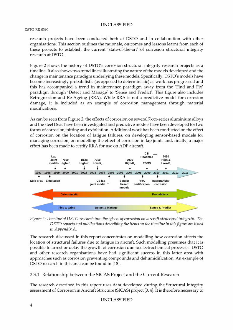
Figure 2 shows the history of DSTO’s corrosion structural integrity research projects as a timeline. It also shows two trend lines illustrating the nature of the models developed and the change in maintenance paradigm underlying these models. Specifically, DSTO’s models have become increasingly probabilistic (as opposed to deterministic) as work has progressed and this has accompanied a trend in maintenance paradigm away from the ‘Find and Fix’ paradigm through ‘Detect and Manage’ to ‘Sense and Predict’. This figure also includes Retrogression and Re-Ageing (RRA). While RRA is not a predictive model for corrosion damage, it is included as an example of corrosion management through material modifications. As can be seen from Figure 2, the effects of corrosion on several 7xxx-series aluminium alloys and the steel D6ac have been investigated and predictive models have been developed for two forms of corrosion; pitting and exfoliation. Additional work has been conducted on the effect of corrosion on the location of fatigue failures, on developing sensor-based models for managing corrosion, on modelling the effect of corrosion in lap joints and, finally, a major effort has been made to certify RRA for use on ADF aircraft.
Deterministic ProbabilisticDeterministic Probabilistic
Find & Grind Detect & Manage Sense & PredictFind & Grind Detect & Manage Sense & Predict
RRAcertification
Exfoliation
D6acHigh-Kt
7050High-Kt
7010Low-Kt
7075High-Kt
ICS lapjoint model
EDMS
Sensorbased
models
Cole et al.
LapJoint
models
Intergranularcorrosion
7050High &Low-Kt
CSIRoadmap
1997 1998 1999 2000 2001 2002 2003 2004 2005 2006 2007 2008 20122009 2010 2011 2013
Figure 2: Timeline of DSTO research into the effects of corrosion on aircraft structural integrity. The
DSTO reports and publications describing the items on the timeline in this figure are listed in Appendix A.
The research discussed in this report concentrates on modelling how corrosion affects the location of structural failures due to fatigue in aircraft. Such modelling presumes that it is possible to arrest or delay the growth of corrosion due to electrochemical processes. DSTO and other research organisations have had significant success in this latter area with approaches such as corrosion preventing compounds and dehumidification. An example of DSTO research in this area can be found in [18]. 2.3.1 Relationship between the SICAS Project and the Current Research
The research described in this report uses data developed during the Structural Integrity assessment of Corrosion in Aircraft Structure (SICAS) project [3, 4]. It is therefore necessary to
UNCLASSIFIED DSTO-RR-0390
UNCLASSIFIED 5
provide an overview of the SICAS project, its major outcomes and its relationship to the current research. The SICAS project was a three-year collaboration between DSTO, CSIRO, BAE SYSTEMS and the then-named University of Wales at Swansea (now Swansea University). It’s goal was to develop a model to predict the effect of pitting corrosion on the fatigue life of the aluminium alloy 7010-T7651. This alloy is of interest as it is the principal structural alloy of the BAE SYSTEMS Hawk Mk 127 fighter aircraft. A fleet of these aircraft entered service with the RAAF in 2000 as fighter trainers. Accordingly, the four partners in the SICAS project undertook an extensive program of specimen corrosion, fatigue testing, fractography and data analysis to determine what, if any, relationship existed between the size of pitting corrosion damage and fatigue life. The size of the pitting corrosion was measured using three metrics: pit width, pit depth and pit cross-sectional area. Statistical analysis, using multiple-stage linear regression, showed that only pit cross-sectional area had a statistically significant effect on fatigue life [3, 4]. This is why the model developed in this report uses the cross-sectional area of the corrosion pits (§4.6) as an input to its fatigue life prediction module. Two sets of fatigue crack growth data for the alloy 7010-T7651 were collected during the SICAS project. One of these was collected using centre crack tension fatigue specimens as per ASTM E647 [19], while the other was collected from the analysis of marker band spacings on low-kt fatigue life specimens designed in accordance with ASTM E466 [2]. The marker band data were found to give more accurate fatigue life predictions during the SICAS project [3, 4] and accordingly it is these data that are used in the current research. The fatigue life specimens used in the current research, both in the model and for the experimental trial, were of identical design as those used in the SICAS project. Several of these specimens were machined during the SICAS project while the remaining were machined afterwards from the same block of 7010-T7651 alloy. A difference between the current research and the SICAS project is that the fatigue life data from the SICAS project is for anodised 7010-T7651 while the specimens tested in the current research were tested with an as-machined surface finish. However, the SICAS project had shown there was minimal difference between the fatigue lives of uncorroded 7010-T7651 regardless of surface condition [3]. In the case of corroded specimens the surface finish again had no significant affect on life as it did not control the initiation or growth of fatigue cracks in the specimens. These were controlled by the corrosion pits which were far larger than the inclusions in the material’s microstructure. The effect was also small for the uncorroded specimens. It was postulated that this was due to the thinness of the anodised layer on the anodised specimens. Finally, the fatigue life predictions made using the model developed in this research are compared to the experimental fatigue lives obtained during the SICAS project (§6.1.1). This was done so that the predictions of the model developed in the current research could be validated.
UNCLASSIFIED DSTO-RR-0390
UNCLASSIFIED 6
2.4 The Effect of Corrosion on the Location of Fatigue Failures
A survey of the literature was made in an effort to find literature regarding the effect of corrosion on the location of fatigue failures in aircraft. Only a few relevant references were found. These are briefly discussed below. The first reference found describes the in-flight failure of the right hand TEF of a RAAF F/A-18 [13]. This is an example of failure from a component that was thought to have an effectively infinite fatigue life and was therefore never scheduled to be inspected. A corrosion pit in the lug that held the TEF to the wing caused it to fail and allowed the flap to separate from the aircraft’s wing. While departing from the aircraft the flap damaged the aircraft’s vertical stabilisers, dorsal deck and left-hand horizontal stabiliser. An investigation by DSTO and the RAAF found two other cracked TEF lugs in the RAAF fleet. In addition, similar failures occurred to F/A-18 aircraft in US Navy and Canadian Forces service. A DSTO investigation found that the AA7050-T7451 material from which the lugs had been manufactured was prone to corrosion pitting which the non-destructive inspection (NDI) technique in use at the time was unable to detect. This failure, and discussion between DSTO and the RAAF [20], prompted DSTO’s ongoing research program in this area [1, 17]. Cook et al. [21] studied the effect of surface corrosion on the fatigue life of specimens containing cold expanded holes. Their study looked at specimens that had been corroded either before (pre-corroded) or after (post-corroded) the application of a cold-hole expansion treatment. They found that the pre-corroded specimens failed in fatigue from corrosion pits that were distant from the hole. These pits were in the diffuse tensile residual stress field that surrounds the compressive stress field near the hole. In contrast to this, the post-corroded specimens failed at the edge of the holes. The corrosion pits in the post-corroded specimens were examined using a SEM and found to be much smaller than those in the pre-corroded specimens. The authors explained this by suggesting that the cold work from pitting affected the evolution of the corrosion pits. It was postulated that the observed difference in pit size caused the observed difference in the location of the critical cracks between the pre- and post-corroded specimens. Cook et al. [21] also investigated the effect of the severity of corrosion on the location of the fatigue failure. This was done exposing specimens to a 0.35% NaCl solution for varying amounts of time. They found that for pre-corroded specimens that as the severity of corrosion increased (i.e. the exposure time was increased) the percentage of failures due to cracks initiated at pits distant from the hole edge increased. Finally, Cook et al. concluded that corrosion did not affect the fatigue endurance of specimens with plain (i.e. untreated) holes. This conclusion contradicts experience at DSTO [22] which has found that post-corroded high-kt specimens have a shorter fatigue life than uncorroded specimens. Mills and Honeycutt [23] examined the fatigue failure of a fuselage frame from a C-141 aircraft. The critical fatigue crack in this fuselage frame initiated from a corrosion pit located in a comparatively low stress region of the fuselage frame. The region was perceived to have an effectively infinite4 life. This is an example of corrosion causing failures in locations that would otherwise be considered immune to fatigue damage. The component’s failure was unexpected and a source of great concern for the USAF which was faced with the prospect of a fleet-wide, and therefore expensive, replacement of the component. Conventional analyses 4 That is, the fatigue life of the region was predicted to greatly exceed the service life of the aircraft.
UNCLASSIFIED DSTO-RR-0390
UNCLASSIFIED 7
gave the component either an infinite life using durability analysis, which assumes a 0.01 inch (250 m) crack, or a life of about 12,000 simulated flying hours, using the starter crack of 0.05 inch crack assumed by damage tolerant analysis. The infinite life was demonstrably untrue given the in-service failure of components at around 35 to 43 thousand simulated flying hours, while the damage tolerant analysis was too conservative as it would have led to expensive and unnecessary inspections. Mills and Honeycutt examined the fatigue-initiating pits in a scanning electron microscope (SEM) and were able to predict a life that corresponded well with the observed in-service life based on their size. This demonstrates the need and value of incorporating corrosion damage into fatigue analyses. Fjeldstad et al. [24] recently published an analysis of the effect of stress fields on the location of fatigue failures in a double-edge notched fatigue specimen. This analysis was based on a model developed by Wormsen et al. [25]. The model was used to predict the location of fatigue failures in a high strength steel. It was implemented as a computer program called P•FAT, which allowed components of arbitrary shape to be modelled. It is a Monte Carlo model which acted as a post-processor for finite element (FE) models created using software packages such as ABAQUS or NASTRAN. These FE models represented the component whose fatigue behaviour was to be predicted. The model then added fatigue initiation sites to the FE model. The size, orientation and location of these sites were determined using statistical distributions. The model treated each initiation site as an equivalent crack oriented normal to the principal stress at its location. It also assumed that these equivalent cracks did not interact. The growth of each of these equivalent cracks was then modelled numerically by calculating the stress intensity around the perimeter of the equivalent crack, incrementing the size of the equivalent crack according to a form of the Paris Law which had been extended to deal with near-threshold fatigue crack growth and then iterating until the crack reached a critical size. The extended form of the Paris Law5 used was:
nth
n KKCdN
da (1)
Where da/dN = fatigue crack growth rate, C = the Paris Law coefficient (2.08 x 10⁻¹⁴ MPa√m), n = the Paris Law exponent6 (4.8) and Kth = fatigue crack growth threshold (4.4 MPa√m).
The numbers in brackets above are the values used by Fjeldstad et al. in their study. These were meant to represent a high strength steel. Note that the prediction of fatigue crack growth in the model was deterministic as only single set values of C, n and Kth were used. The model was able to predict the growth of surface, embedded and corner cracks and could also manage the transition between these crack types. For example, an embedded crack would be changed to a surface crack if it intersected the surface of the component. Unfortunately, the model’s predictions were not compared with experimental results for the material modelled. Despite this the model is of interest to DSTO as it is similar to the model implemented in this report. Fjeldstad et al., however, did not address the effects of corrosion on fatigue initiation
5 The standard form of the Paris Law is described in §2.5.2.1. 6 Note that Fjeldstad et al. [24] used ‘m’ rather than ‘n’ for the Paris Law exponent. ‘n’ is used here for consistency with later sections of this report, in particular §2.5.2.1.
UNCLASSIFIED DSTO-RR-0390
UNCLASSIFIED 8
site or fatigue life in their model. However, their model could easily be modified to simulate the effects of corrosion damage by introducing a second size distribution of crack initiation sites to represent corrosion pits. Finally, a NATO Research and Technology Organisation report [26] mentions on page 5-15 that extrinsic damage such as corrosion can change the failure modes and location of aircraft structures as part of a discussion of modelling the physics of fatigue failures in aircraft. The example given relates to pitting corrosion leading to intergranular corrosion, which then leads to reductions in fatigue life and fatigue failures in unexpected locations. This same reference also notes (on page 6-39) that the effects of extrinsic damage types such as corrosion on structural integrity and endurance are difficult to predict. 2.5 The Simulation of Fatigue Crack Growth
2.5.1 Introduction
Given the critical nature of fatigue failures in aircraft, models that simulate the growth of fatigue cracks and predict fatigue lives are commonplace. These models range from simple equations such as Miner’s Law for variable amplitude fatigue lifeing [27] and the Frost-Dugdale equation for fatigue crack growth [28] all the way through to complex models that attempt to simulate the behaviour of multiple grains and inclusions using FE modelling [29-31]. There is even a model proposed by the US Air Force Research Laboratory (AFRL) and others, called the Digital Twin, to simulate an entire aircraft down to the microstructural scale by 2025 [32]. Some models have gone even further than this and have simulated the behaviour of a collection of individual atoms into which a model crack is introduced [33]. In the middle of this range lie the commonly used models of fatigue behaviour based on continuum mechanics and linear elastic fracture mechanics (LEFM). These include the Paris Law7 [34] and its various descendants such as the Forman [35], NASGRO [36] and Walker [37] equations. These LEFM-based models are typically implemented as computer programs. The most prominent of these are AFGROW [38], NASGRO [36] and FASTRAN [39]8. DSTO has developed a variant of FASTRAN, called CGAP, which has extensions to allow the probabilistic modelling of fatigue crack growth [40]. The LEFM-based models are often combined with a crack closure9 model to allow the effects of crack retardation due to variations in loading to be incorporated into the model. Regardless of their complexity all of these models are empirical and require calibration using data from actual materials tests.
7 Note that the term ‘Paris Law’ is a misnomer in that the Paris Law equation is an empirical relationship and not a law (such as the law of conservation of energy) in the scientific sense of the word. However, the convention is to refer to this equation as the ‘Paris Law’ and this convention will be followed in this report. 8 Note that many aircraft OEMs have developed in-house fatigue crack growth prediction programs. As these are not widely available their use is not considered in this report. 9 Crack closure is the phenomenon where the faces of a growing fatigue crack come into contact at positive loads. There are numerous crack closure mechanisms. A brief overview of these mechanisms can be found in Suresh [41].
UNCLASSIFIED DSTO-RR-0390
UNCLASSIFIED 9
In addition to their complexity, fatigue models can also be distinguished by whether they are deterministic or probabilistic. In general, older models have tended to be deterministic while newer models are more likely to be probabilistic. The deterministic models use safety factors to deal with the scatter inherent in fatigue processes. In contrast, the probabilistic models incorporate this scatter into their controlling parameters (though safety factors may still be used for reasons of design conservatism). Therefore, the controlling parameters of these probabilistic models are represented as distributions rather than discrete values. Many of these probabilistic models use a Monte Carlo approach to achieve this. The perceived advantage of probabilistic models is that they may be able to more accurately model the inherent scatter in fatigue life, fatigue crack growth rates, fracture toughness, yield stress and resistance to crack initiation. Therefore using probabilistic models may reduce the risk of catastrophic failure. This will allow the use of lower safety factors which will in turn reduce the cost of operating aircraft and other machines subject to fatigue damage. The remainder of this section discusses some of the models mentioned above. The purpose of this discussion is to show how the modelling method used in this report relates to past work in the literature. Conversely, some of the models discussed below are included to show why they were not used in this report.
2.5.2 Models using Linear Elastic Fracture Mechanics and K
This section briefly examines the Paris Law, from which most other fatigue crack growth laws have been derived10; the Walker equation, which is used by AFGROW; and the Harter-T method, which is used by AFGROW for tabulated fatigue crack growth rate data and which is based on the Walker equation. It should be noted that all of these models are for predicting crack growth under constant amplitude loading conditions. They must be modified using retardation models for predicting fatigue lives under variable amplitude loading conditions. Retardation models are not discussed in this report as all testing was conducted under constant amplitude loading conditions. 2.5.2.1 The Paris Law11 In 1913 Inglis determined the stress distribution near an ellipse [43]. He found that as the ellipse tended towards a slit that the stress at its points tended to infinity. In 1957 Irwin used this result to define the stress intensity factor, K, a scalar quantity that quantifies the severity of the stress field around a crack [44]. Paris et al. [34] then used the cyclic stress intensity factor12, K, to correlate the growth rates of fatigue cracks in metals. They found that the crack growth rate increased with increased K and that results from different specimen geometries could be reconciled on this basis. The equation they proposed, in modern notation, was:
10 The Frost-Dugdale equation [28] is an exception to this. 11 The text in this section is partly based on Crawford, 1996 [42] 12 The cyclic stress intensity factor is defined as: ΔK = Kmax - Kmin, where Kmax is the maximum stress intensity during a fatigue cycle and Kmin is the minimum.
UNCLASSIFIED DSTO-RR-0390
UNCLASSIFIED 10
nKCdNda (2)
where C = the Paris Law Factor, n = the Paris Law Coefficient, K = the Cyclic Stress Intensity Factor = f(, specimen geometry, crack size), = stress range = max – max,, and min, max = the minimum and maximum cyclic stresses, respectively. While useful the Paris Law cannot account for the effect of load ratio (R) on crack growth rates. It also cannot deal with near-threshold or near-fast fracture crack growth. As such further models were developed which introduced additional parameters to deal with these issues. These were the Forman [35], NASGRO [36] and Walker [37] equations mentioned above. The Walker equation, which is used in this report, is described in detail in the next section. 2.5.2.2 The Walker Equation The Walker equation was proposed by Walker for positive values of R in 1968 [37]. Walker found that it was useful for fitting fatigue crack growth data for the aluminium alloys 2024-T3 and 7075-T6. It was subsequently extended to negative load ratios. As such there are two branches of the equation. One is for positive load ratios and the other is for negative load ratios. The combined form of these equations is [38]:
0for1
0for1)1(
max
)1(
RRKC
RRKCdN
daw
w
nmn
nmn (3)
where K is as defined for the Paris Law (Equation x), Cn and nw are fitting coefficients, R = the load ratio = Kmin/Kmax, and m = the Walker exponent.
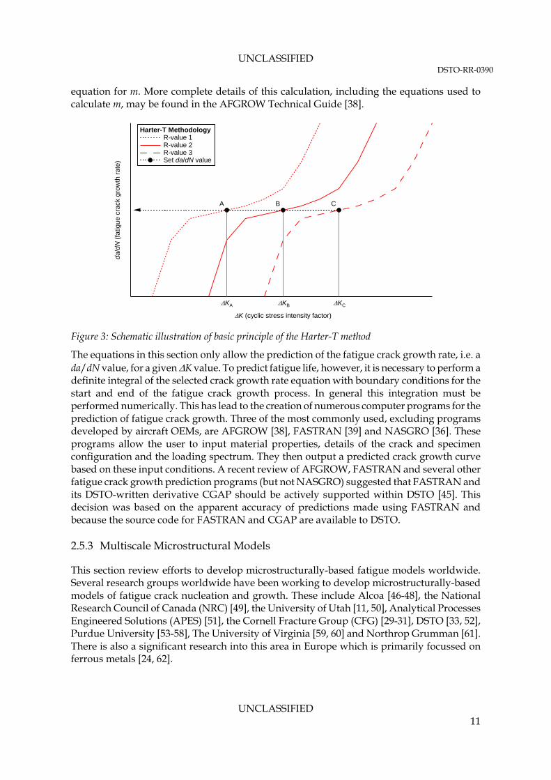
Walker found that the exponent, m, had a value of 0.5 for 2024-T3 and 0.425 for 7075-T6. It should be noted that, however, m is a fitting parameter and is not a material property [38]. It has no physical significance. 2.5.2.3 The Harter-T Method The Harter-T method [38] has been described as a ‘point-wise’ implementation of the Walker equation. It was developed by James Harter in 1983 at USAF-AFRL [38]. It is the method used to calculate the fatigue life tables described in §4.9 of this report. The basic principle of the Harter-T method is that a value of the exponent m is calculated for every adjacent pair of fatigue crack growth data points at a given value of da/dN. This is illustrated in Figure 3 in which there are two adjacent pairs of points, AB and BC13. Given that da/dN is the same for both points in the pair, it is possible to use the Walker equation, above, to calculate the m value for that pair of data points by equating the crack growth rates and solving the resultant
13 The pair AC is ignored as the curves from which these points come are not adjacent.
UNCLASSIFIED DSTO-RR-0390
UNCLASSIFIED 11
equation for m. More complete details of this calculation, including the equations used to calculate m, may be found in the AFGROW Technical Guide [38].
K (cyclic stress intensity factor)
da/d
N (
fatig
ue c
rack
gro
wth
rat
e)
Harter-T Methodology R-value 1 R-value 2 R-value 3 Set da/dN value
A B C
KA KB KC
Figure 3: Schematic illustration of basic principle of the Harter-T method
The equations in this section only allow the prediction of the fatigue crack growth rate, i.e. a da/dN value, for a given K value. To predict fatigue life, however, it is necessary to perform a definite integral of the selected crack growth rate equation with boundary conditions for the start and end of the fatigue crack growth process. In general this integration must be performed numerically. This has lead to the creation of numerous computer programs for the prediction of fatigue crack growth. Three of the most commonly used, excluding programs developed by aircraft OEMs, are AFGROW [38], FASTRAN [39] and NASGRO [36]. These programs allow the user to input material properties, details of the crack and specimen configuration and the loading spectrum. They then output a predicted crack growth curve based on these input conditions. A recent review of AFGROW, FASTRAN and several other fatigue crack growth prediction programs (but not NASGRO) suggested that FASTRAN and its DSTO-written derivative CGAP should be actively supported within DSTO [45]. This decision was based on the apparent accuracy of predictions made using FASTRAN and because the source code for FASTRAN and CGAP are available to DSTO. 2.5.3 Multiscale Microstructural Models
This section review efforts to develop microstructurally-based fatigue models worldwide. Several research groups worldwide have been working to develop microstructurally-based models of fatigue crack nucleation and growth. These include Alcoa [46-48], the National Research Council of Canada (NRC) [49], the University of Utah [11, 50], Analytical Processes Engineered Solutions (APES) [51], the Cornell Fracture Group (CFG) [29-31], DSTO [33, 52], Purdue University [53-58], The University of Virginia [59, 60] and Northrop Grumman [61]. There is also a significant research into this area in Europe which is primarily focussed on ferrous metals [24, 62].
UNCLASSIFIED DSTO-RR-0390
UNCLASSIFIED 12
Many of these North American research programs fall under the umbrella of the ‘Structural Integrity Prognosis System’ (SIPS) project [63]. This is a project sponsored by the US Defence Advanced Research Projects Agency (DARPA). SIPS is intended to develop models to predict the structural integrity of individual aircraft as a function of their usage, materials and environment. Papazian et al., said that SIPS is [63]:
‘…founded on a collaboration between sensor systems, advanced reasoning methods for data fusion and signal interpretation, and modeling and simulation systems…’.
The modelling approach used in SIPS combines models for corrosion with those for fatigue damage. These models are based on statistical representations of the microstructure of the material being modelled combined with models of the processes of corrosion and fatigue in the material. The corrosion and fatigue models used are mechanistic rather than empirical as the intention is to model real material behaviour. Several of the groups listed above (viz. NRC, Hoeppner et al. and APES) are working together on a program called the Holistic Structural Integrity Process (HOLSIP), which they have envisaged as a successor to the Aircraft Structural Integrity Program (ASIP) of the US Air Force (USAF) [64]. This section will give a brief overview of the work of each of the groups mentioned above. 2.5.3.1 Alcoa In the early 1990s Magnusen et al. [46-48] of Alcoa studied the effect of the microstructure of the aluminium alloy 7050-T7451 on its fatigue crack growth behaviour. The purpose of their work was to develop a model that could predict the effect of varying the microstructure of the model material while avoiding the time consuming and expensive testing of variant materials. Fatigue testing was conducted using both low and high-kt specimens. The four variants of the alloy tested were ‘old material’, ‘now material’, ‘low porosity material’ and ‘thin material’. The materials differed in terms of the microporosity and inclusions they contained and their grain size distributions. An extensive study of these properties and of the fatigue life behaviour of the material can be found in [47]. Fatigue life tests showed that the thin material had the longest fatigue lives followed by the low porosity material, the now material and the old material, which had the shortest fatigue lives. The spatial and frequency distributions of the inclusions and microporosity were determined using metallographic sections of each alloy. The inclusions were randomly distributed through the microstructures of the material while the microporosity was concentrated near the centre of the materials’ cross-sections [46]. The low porosity material and the thin material had far less porosity than the old and now materials. The spatial distribution of the inclusions means that, in high-kt specimens, there will always be inclusions in the volume of highly stressed material near the stress concentrating feature. In contrast, it is comparatively unlikely that any microporosity will be in this volume of material. This means that the effect of microporosity on the fatigue life of high-kt specimens will be reduced. The effect of microporosity is therefore similar to the effect of pitting corrosion as the effect of either on fatigue life depends on its locations. However, Magnusen et al. [46] state, based on Trantina and Barishpolsky [65], that when microporosity is present in the high stress volume it is the dominant driver of initial short crack growth as microporosity has a higher associated stress concentration than inclusions at a given size.

UNCLASSIFIED DSTO-RR-0390
UNCLASSIFIED 13
The modelling of fatigue crack growth was conducted using a custom written software package which used the standard Raju and Newman stress intensity factor solutions [66]. A Monte Carlo simulation was added to this by varying the values of the input parameters of defect size and fatigue crack growth rate using a probabilistic modelling package call PROBAN14. An example of the fatigue life predictions made by this software for high-kt specimens is shown in Figure 4 below. The match between the experimental results and the predictions of the model is excellent.
220
200
180
160
140
120
100
Net
Sec
tion
Str
ess
(MP
a)
104
105
106
107
Fatigue Life (Cycles)
Magnusen et al.Old 7050-T7451
Experimental Results Model (p = 0.5) Model (p = 0.05 & p = 0.95)
Figure 4: Fatigue life predictions for uncorroded high-kt fatigue life specimens from Magnusen et al.[46, 47] for old-manufacture (i.e. pre-1984) 7050-T7451.
2.5.3.2 National Research Council of Canada, The University of Utah and APES The National Research Council of Canada has been working with Professor David Hoeppner and his research group at the University of Utah and with Analytical Processes Engineering Solutions on fatigue processes in aircraft for many years. These three groups have been developing a so-called ‘Holistic Structural Integrity Process (HOLSIP) to supplement or replace the current Aircraft Structural Integrity Program (ASIP) [64] which was developed by the USAF in September 1972 after the crash of USAF F-111 67-049 after approximately 100 flying hours in December 1969 [67]. The rationale behind HOLSIP is that while ASIP does have requirements to deal with corrosion and several other degradation modes, these are not sufficiently developed [51] and do not account for all possible failure modes in aircraft. Therefore, a fundamental tenet of HOLSIP is that all stages of the fatigue degradation process of a given material should be modelled accurately with reference to the features of that material’s microstructure. These stages are, according to Merati and Eastaugh, fatigue crack nucleation, short crack growth, long crack growth, and fracture [68]. This tenet is encapsulated in a concept called the ‘Initial Discontinuity State’ (IDS) which is intended to
14 PROBAN is distributed by Det Norske Veritas (DNV) at http://www.dnv.com/services/software/products/safeti/safetiqra/proban.asp
UNCLASSIFIED DSTO-RR-0390
UNCLASSIFIED 14
describe the material’s microstructure in its as-manufactured state. The IDS can be viewed as a replacement for the Equivalent Initial Flaw Size (EIFS) used in ASIP. An IDS differs from an EIFS, however, as it is derived from the material’s microstructure and is, according to Liao et al. [69], ‘physics-based’ rather than from curve fitting to fatigue life data, which is typically how EIFS values are determined. As the material is damaged by fatigue, corrosion or some other degradation process this IDS is replaced by a ‘Modified Discontinuity State’ (MDS). A review of the IDS and MDS concepts can be found in Crawford [70]. Merati and Eastaugh examined the relationship between the nucleation of fatigue cracks in aluminium alloys 7075-T6 and 7079-T6 [71]. Three forms of the 7075-T6 alloy were studied. These were (i) new material rolled to thicknesses of 1.6 and (ii) 4.0 mm thicknesses and (iii) old 4.1 mm thick extruded material which had not been used. The 7079-T6 material was rolled to a thickness of 1.7 mm and was unused. The old materials were harvested from unused aircraft components. The inner faces of these materials were both anodized; while the outer surface of the used 7075-T6 was anodised and the outer surface of the 7079-T6 was clad and anodized. The study conducted by Merati and Eastaugh [71] consisted of three stages. These were microstructural analysis, fatigue testing and fractography. The microstructural analysis found that the 4.0 mm thick uncoated 7075-T6 had a gradient in particle size, with the mean size of particles being higher in the material’s centre than at its edge. None of the other materials in this study showed this trend. This includes the 4.1 mm thick extruded material. In all cases the thinner materials contained smaller particles. Fatigue testing showed that the coating on the old material reduced the scatter in fatigue lives. The scatter in the fatigue lives of the uncoated specimens was large enough to obscure any effect of thickness. In contrast, for the coated materials there was minimal scatter in fatigue lives and the thinner material has much longer fatigue lives than the thick material. Fractography showed that the coated materials consistently failed from cracks nucleated in the surface coating while the uncoated material failed from cracks nucleated from inclusions. Shekhter et al. observed a similar behaviour in uncorroded high-kt specimens of clad 7075-T6 [52]. However, they also observed that fatigue cracks nucleated from corrosion pits in pre-corroded high-kt specimens of this material. This suggests there is a feature size between the inclusions 7075-T6 and corrosion pitting at which the effect of the clad layer on crack nucleation is overcome by the effect of the corrosion pits. Merati conducted a similar study on 2024-T3 in clad and unclad states and observed the same crack nucleation behaviour as for 7075-T6 and 7079-T6. Specifically, in the unclad material crack nucleation occurred at inclusions, typically those containing iron, while in the clad material multiple crack nucleation sites were observed in the clad layer and the inclusions played no role in crack nucleation. Subsequently, Liao et al. of NRC published a combined experimental and modelling study of short-crack growth in unclad 2024-T351 [69]. Short-crack growth is the stage after fatigue crack nucleation in the stages listed by Merati and Eastaugh [71]. The objectives of this study were to develop deterministic and probabilistic models of short crack growth in 2024-T351. These were then combined with a long crack growth model to predict the fatigue life of the tested specimens. The inputs to these models were the fatigue lives of a series of test specimens and fractography data from these specimens of the size of the critical fatigue crack nucleating inclusion. The size of the inclusions was represented by their maximum width and

UNCLASSIFIED DSTO-RR-0390
UNCLASSIFIED 15
maximum length. No correlation was observed between the width and length of these particles. As part of this work, Liao et al. developed two probabilistic models which both used AFGROW to predict fatigue crack growth. The first model had two random variables, particle length and particle width. The second model had an additional random variable, KIDS, which represents the stress-intensity-factor limit for an initial/discontinuity-state/particle-induced crack. This third random variable, with some optimisation, means that the second model can predict the mean and scatter of the observed fatigue lives. KIDS appears to be analogous in effect to the crack metric ratio (CMR) developed by Crawford et al. [3, 4] for corrosion pitting in 7010-T7451 in that it allowed microstructural factors other than pit or particle size to be incorporated into modelling. Examples of such factors include grain size, grain orientation the resistance of grain boundaries to cracks growing through them [69]. Hoeppner and colleagues at the University of Utah have conducted extensive research into the effects of pitting corrosion [50, 72-79] and fretting15 [72, 73, 80-88] on the fatigue life of aircraft. The published work on corrosion pitting has concentrated on 2024-T3 [76, 79] and 7075-T6 [50, 77, 78]. As an example, Jones and Hoeppner have looked at the effect of both prior corrosion [50] and ‘concomitant corrosion’16 [78] on the fatigue behaviour of 7075-T6. They have also examined the effect of prior corrosion on the fatigue behaviour of 2024-T3 [76]. These papers concluded that pit surface area and the proximity of other pits were as important as pit depth in their effect on fatigue life. 2.5.3.3 Cornell University The Cornell Fracture Group at Cornell University have been developing finite and boundary element models of fatigue and fracture processes in materials for several decades. This has primarily been under the guidance of Professor A. R. Ingraffea who is currently the head of the Cornell Fracture Group. The work of this group is of interest as they are attempting to simulate materials from the microscopic to the macroscopic scale. Since 1999, the group’s models have often been based on virtual microstructures [89]. A virtual microstructure is a FE model of a material’s microstructure which is generated from statistical representations of the size, locations and shape of the grains and inclusions which constitute the material being simulated. The crystallographic texture of the grains (i.e. orientation) is also considered. The statistical representations of the grains and inclusions come from quantitative metallographic analysis of the material being modelled. The texture is measured using an SEM equipped with an EBSD17 detector. Each grain and inclusion is then modelled as a separate FE model. These separate
15 Hoeppner’s work on fretting is outside the scope of this report and so will not be discussed in this report. 16 ‘Concomitant corrosion’ is the term used by Hoeppner and his co-workers to describe corrosion that is occurring at the same time as fatigue crack growth. It is more commonly referred to as ‘corrosion fatigue’. 17 EBSD = Electron Back Scatter Diffraction, a form of electron diffraction pattern analysis that can detect the orientation of grains on the surfaces of materials examined in an SEM.

UNCLASSIFIED DSTO-RR-0390
UNCLASSIFIED 16
models was then joined together using constitutive functions which describe how the interfaces between the grains and inclusions behave. The very large number of papers published by the Cornell Fracture Group prevents an exhaustive examination of their work. Therefore, a recent series of three papers from this group will be examined instead [29-31]. These papers are concerned with the formation of microstructurally small fatigue cracks from cracked inclusions in the aluminium alloy 7075-T7651. While these papers do not directly address the formation of fatigue cracks from corrosion, they are of interest as the modelling processes used are still relevant. The first of the three papers reviewed here, Bozek et al [29], develops a probabilistic model of the fracture of the inclusions in 7075-T7651. This model consists of a cube of elastic-viscoplastic material which has a purely elastic semi-ellipsoidal particle embedded into one face. The cut surface of the particle is flush with one face of the cube. The model allowed the effects of matrix strain, matrix orientation, particle size, particle aspect ratio, particle intrinsic flaw size and boundary constraint to be modelled. The model was used to predict particle strength and stress distributions which were compared to give the frequency of particle fracture. This frequency was then compared to experimental results for particle fracture in two single-edge notched samples of 7075-T651. The model predicted that between 2.2% and 4.9% of the particles in the material would fracture. An experimental trial conducted on two specimens gave a mean of 4.5%. Uncracked particles can be removed from subsequent modelling which reduces the computational demands of this modelling [30, 31]. The second paper in this series, Hochhalter et al. [30], models the nucleation of matrix fatigue cracks in 7075-T7651 from cracked inclusions. As with Bozek et al. [29] this paper is a combined experimental and modelling study. The modelling study in this paper examines five different metrics for predicting crack nucleation. The first three of these were based on plastic slip. The fourth was the maximum energy expended on a given slip plane. The last metric was based on both crystallographic plastic slip and the tensile stress on a slip plane. A range of metrics was examined as it was not clear beforehand which would be the most applicable. These metrics were non-local as they were applied over an arc centred on the crack tip. This was necessary as the stress singularity at the crack tip could not be modelled directly. Hochhalter et al developed two models in his paper. The first was a baseline model similar to the model used by Bozek et al. [29]. This was used to study and optimise the five metrics. The second model replicated several fractured inclusion and its surrounding matrix from a test specimen. As no measurements were made into the depth of the material the modelled inclusions and matrix were assumed to be of constant thickness of 74 m normal to the plane of the surface. The orientation of the grains was modelled using EBSD data from the real material. The experimental study in Hochhalter et al. [30] consisted of fatigue testing of double edge notched fatigue specimens for 3,000 cycles at R = 0.1. Only a small percentage of the inclusions in the material fractured. The initiation and growth of fatigue cracks from the 55 cracked inclusions was recorded in the notch root of the specimens. The fractured inclusions were typically larger than the mean size of all inclusions, which suggests that the larger particles were more prone to fracture. Crack growth was typically normal to the loading direction but changed at grain boundaries. About 73% of the cracked inclusions and initiated micro-cracks
UNCLASSIFIED DSTO-RR-0390
UNCLASSIFIED 17
by 300 loading cycles. After testing, EBSD was used to analyse the orientation of the grains through which the initiated fatigue cracks grew. The last paper in the series [31] consolidates the models developed in the previous two papers into a semi-empirical model based on FE analysis that predicts the number of cycles required for the nucleation of a fatigue crack. The FE model is needed to calculate the local stress at the particles in the model and the rate of slip accumulation in the grains near the particles. 2.5.3.4 Purdue University In the last decade or so the research group at Purdue University in the US led by Professor Hillberry has conducted extensive research into the effect of microstructural inclusions and corrosion pits on the fatigue behaviour of 2024-T3 and 7075-T6 aluminium alloys commonly used in aircraft structures. This includes the work of DeBartolo [53, 90, 91], Laz [55, 56, 92], Gruenberg [93-96] and van der Walde [24, 57, 97, 98]. DeBartolo’s [53 , 90, 91] only mentions corrosion briefly. She was primarily concerned with modelling fatigue crack growth in 2024-T3, 2524-T318 and 7075-T6. To achieve this, DeBartolo characterised the size distributions of the inclusions in these alloys and then combined these data with good quality fatigue crack growth data from various literature sources to predict their fatigue lives using FASTRAN. Fatigue cracks generally nucleated from cracked inclusions. Most of these cracked inclusions contained iron and were typically larger than the average inclusion size. This latter observation indicates that larger inclusions were more fracture prone. The fatigue crack predictions made using these particles and FASTRAN slightly overestimated the experimental fatigue lives observed. Van der Walde and Hillberry [57] developed a model to predict the fatigue life of 1.6 mm thick sheets of 2024-T3 that had been corroded prior to fatigue testing. This material was the same material previously used by Gruenberg et al. [54]. Samples of this material were corroded by exposure to an aqueous solution of NaCl and H2O2 as per ASTM G11019 [99]. Once corroded the material was serially sectioned to find and measure the corrosion pits that resulted from the corrosion exposure. This is in contrast to Crawford et al. [3, 4] and many other researchers who have used only the largest corrosion pits on the fatigue fracture surfaces. Van Der Walde noted that his method, which uses effectively random planes, may give a different pit size distribution to measuring the corrosion pits that appear on fracture surfaces. The width depth and area of the corrosion pits were determined using digital image analysis. Semi-elliptical cracks of equivalent area and aspect ratio were then fitted to the corrosion pits. This geometric model of the corrosion pits is similar to that used in the SICAS project [3, 4]. These equivalent semi-ellipses described above were located so that their origin was located at the surface origin of the corrosion pits they represented. The size, shape and locations of these
18 Note that 2524-T3 is a compositionally and microstructurally cleaner variant of 2024-T3 and is intended as a replacement for same. 19 The corrosion solution consisted of 57 g NaCl and 10 ml of 30% H2O2 made up to a volume of one litre using water. This is approximately a 1 Molar solution of NaCl. The H2O2 was added to acidify the solution and thereby increase its corrosivity.
UNCLASSIFIED DSTO-RR-0390
UNCLASSIFIED 18
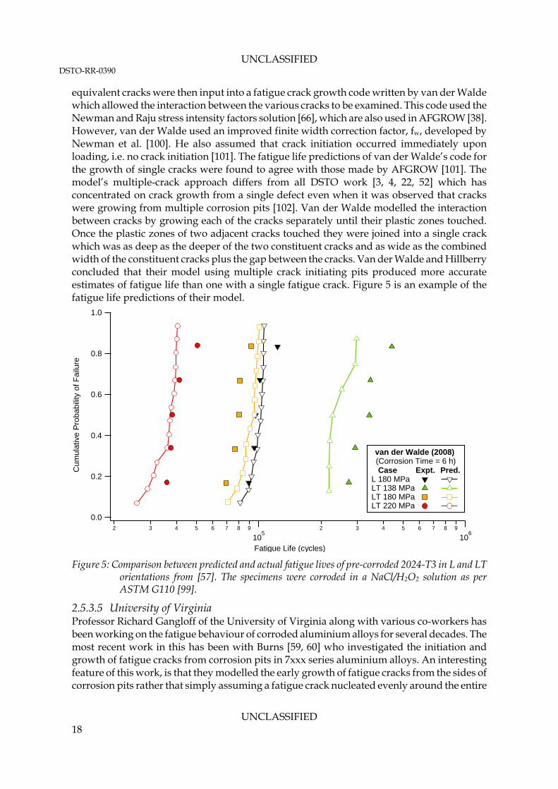
equivalent cracks were then input into a fatigue crack growth code written by van der Walde which allowed the interaction between the various cracks to be examined. This code used the Newman and Raju stress intensity factors solution [66], which are also used in AFGROW [38]. However, van der Walde used an improved finite width correction factor, fw, developed by Newman et al. [100]. He also assumed that crack initiation occurred immediately upon loading, i.e. no crack initiation [101]. The fatigue life predictions of van der Walde’s code for the growth of single cracks were found to agree with those made by AFGROW [101]. The model’s multiple-crack approach differs from all DSTO work [3, 4, 22, 52] which has concentrated on crack growth from a single defect even when it was observed that cracks were growing from multiple corrosion pits [102]. Van der Walde modelled the interaction between cracks by growing each of the cracks separately until their plastic zones touched. Once the plastic zones of two adjacent cracks touched they were joined into a single crack which was as deep as the deeper of the two constituent cracks and as wide as the combined width of the constituent cracks plus the gap between the cracks. Van der Walde and Hillberry concluded that their model using multiple crack initiating pits produced more accurate estimates of fatigue life than one with a single fatigue crack. Figure 5 is an example of the fatigue life predictions of their model.
1.0
0.8
0.6
0.4
0.2
0.0
Cum
ulat
ive
Pro
babi
lity
of F
ailu
re
2 3 4 5 6 7 8 9
105
2 3 4 5 6 7 8 9
106
Fatigue Life (cycles)
van der Walde (2008) (Corrosion Time = 6 h)
Case Expt. Pred. L 180 MPa LT 138 MPa LT 180 MPa LT 220 MPa
Figure 5: Comparison between predicted and actual fatigue lives of pre-corroded 2024-T3 in L and LT
orientations from [57]. The specimens were corroded in a NaCl/H2O2 solution as per ASTM G110 [99].
2.5.3.5 University of Virginia Professor Richard Gangloff of the University of Virginia along with various co-workers has been working on the fatigue behaviour of corroded aluminium alloys for several decades. The most recent work in this has been with Burns [59, 60] who investigated the initiation and growth of fatigue cracks from corrosion pits in 7xxx series aluminium alloys. An interesting feature of this work, is that they modelled the early growth of fatigue cracks from the sides of corrosion pits rather that simply assuming a fatigue crack nucleated evenly around the entire

UNCLASSIFIED DSTO-RR-0390
UNCLASSIFIED 19
periphery of the corrosion pit. To achieve this they modified the classic Newman and Raju K-solution [66] which they called the ‘Modified Bump’ K-solution. These pit-initiated fatigue cracks then grew around the pit and merged with other cracks initiated by the pit, if any, to form a continuous crack front that enveloped the entire pit from which they had originated. This behaviour was detected by using a marker band spectrum during fatigue testing and quantitative fractography post-testing. Fatigue cracks were observed to form at small features around the periphery of the corrosion pits which pushed the pit’s periphery either in or out. Note that the corrosion pits examined by Burns were not produced by conventional means. Instead the surface of the specimens was masked with tape. Three circular holes were then cut into this tape and the corrosive solution was applied through this holes. A potentiostat was then used to apply a controlled current for a given time to the specimen to drive the corrosion process. The modelling of crack growth undertaken by Burns et al. showed that the number of cycles required to create a fatigue crack from a corrosion pit decreased to zero as the applied stress was increased. Burns et al. stated that this validates the assumption of zero initiation cycles that is intrinsic in ECS modelling. 2.5.4 The Weakest Link Theorem
The model developed in this report is a ‘Weakest Link’ model in that specimen failure occurs when any single element of the specimen fails. The elements in the model are the inclusions and corrosion pits from which cracks initiate. The model assumes that the corrosion pit or inclusion that produces the shortest predicted life controls the life of the model specimen. The original development of the weakest link model is attributed to Weibull [103, 104] Weakest link models are widely used to describe the fracture behaviour of brittle materials. The model is particularly suited to brittle materials such as ceramics where there is minimal crack growth between crack initiation and unstable fracture. The fracture behaviour of these materials is therefore controlled by the behaviour of the crack initiating features they contain. This in turn is controlled by the size of these features and the stress they are under. The mathematics of the Weibull weakest link theory can be summarised as follows [104]: Given a failure probability of (Pf)i for a given element of volume V in a component, the survival probability of that element is 1 - (Pf)i. The probability of survival for the entire component, encompassing all of its n elements is therefore20:
if
n
iif
n
iif
n
iis
n
iS PPPPP
1111
expexp1 (4)
Where Ps = the probability of survival, (Pf)i = probability of failure for element i of the component, n = total number of defects
20 Note that capital Pi, Π, in this context is the mathematical notation for the product of a series of terms. It is analogous to Σ for summation of a series of terms.
UNCLASSIFIED DSTO-RR-0390
UNCLASSIFIED 20
Equation (4) assumes that the stress state in the volume element V varies only slowly. This means that a weakest link model such as that developed in this report must divide the component being modelled into regions that are small enough that each of these regions can be considered to be uniformly loaded. Therefore, the volume elements for components with comparatively shallow stress gradients, such as the low-kt fatigue coupons modelled in this work, can be larger than those for components with high stress gradients such as a high-kt fatigue coupon. The Weakest Link theory as represented by Equation (4) was developed for brittle materials. Therefore Ps is the probability of survival (i.e. not fracturing) of a brittle component as a function of the applied stress. However, Weakest Link theory has also been applied to the fatigue of materials based on the assumption that the first defect in a material specimen to initiate a crack will cause that specimen to fail. In this case, the survival probability, Ps, is typically the probability of a component surviving a given loading for a given duration of fatigue loading. Karlen et al. [103] used three different methods to estimate the fatigue notch factor of the welding steel Weldox 420. The methods used were the classical notch root analysis methods of Neuber, Peterson and Heywood; the Weakest Link integral as defined by Weibull [100, 101] and a stochastic method using randomly sized and distributed inclusions, which were treated as cracks. They found that the size distributions of the inclusions were calculated using two methods which were called the Block Maximum (BM)21 method and the ‘Peak Over Threshold’ (POT)22 method. These methods were also used in the SICAS project to analyse corrosion pit size data during the development of the corrosion protocol used in that project [3, 4]. Wormsen et al. also mentioned the problems caused by the ‘corpuscle problem’ where the size of three dimensional objects, the inclusions in the steel being tested, are characterised using two-dimensional measurements of their size on polished planes [25]. Finally, their model was able to predict the location of fatigue failures in their model specimens. They modelled both low-kt and high-kt specimens. They found that the fatigue failure locations in the low-kt specimens were spread along the gauge length of the specimens and that there were a significant number of sub-surface crack initiations. In contrast, the high-kt specimens failed entirely on the surface of the specimens in a tight band around the highest stressed region of the high-kt specimen’s gauge section. 2.6 Pit Sizes Reported in the Literature
DSTO experience has shown that there are no NDI technologies that can measure the size of pitting corrosion in aluminium alloys with the required accuracy [22]. Unless new NDI technologies arise in the near future it will therefore be necessary to assume a pit size distribution based on tear down and maintenance data supplemented by laboratory and
21 The ‘Block Maximum’ method characterises defect sizes by dividing a polished plane of the material into k area. The largest particle in each of these areas is then found and the results from each area are ranked. From this ranking the parameters of an extreme maximum size distribution are fitted. 22 In the ‘Peak over Threshold’ method all of the particles on a polished plane of the material above a threshold size are measured. These measurements are then used to fit an extreme maximum size distribution.
UNCLASSIFIED DSTO-RR-0390
UNCLASSIFIED 21
exposure site data if models similar to that developed in this report are to be used in service. To this end, the literature was surveyed to find the pit size metrics commonly used to quantify pit size in 2xxx and 7xxx-series aluminium alloys. The most commonly used pit size metrics were depth, width and cross-sectional area. Of these, pit depth was by far the most commonly used pit metric. Figure 6 shows histograms for the mean and maximum pit depths reported. These values are predominantly from laboratory test programs but there are a small number of in-service data reported. Note that in comparing the two parts of this figure that not all data sources quoted both mean and maximum pit depths. See Appendix B for the data sources in this figure. As the data sources in Figure 6 typically do not provide all of the original data used to calculate the reported pit metrics it was not possible to determine if the measurements techniques used in each source were consistent. Despite this Figure 6 is a useful indication of the range of pit depths reported in the literature. It indicates the pit depths obtained by DSTO in its work in this area [3, 4, 22, 52] are near the median of the mean and maximum pit depths reported in the literature. Figure 7 plots the cumulative density function (CDF) distributions for mean and maximum pit depth together. The mean pit depth axis (top) has half the range of the maximum pit depth axis (bottom). When plotted this way the two CDF overlay each other. This suggests that the maximum pit depth is twice the mean pit depth. A similar behaviour is apparent with the DSTO-collected pit depth data, Figure 8. However, as shown by the width of the confidence interval, it is not apparent for the remaining data, from sources external to DSTO, in this figure. This behaviour has been reported here only to note its existence. Its significance or otherwise has not yet been determined. The authors are planning to investigate whether this behaviour can be used in modelling. In the mean time, this relationship should not be used in fatigue life prediction models until this investigation has been completed.
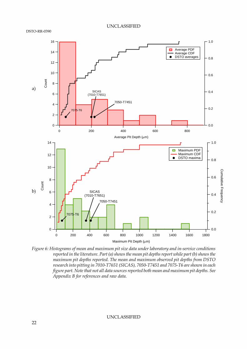
UNCLASSIFIED DSTO-RR-0390
UNCLASSIFIED 22
a)
16
14
12
10
8
6
4
2
0
Cou
nt1.0
0.8
0.6
0.4
0.2
0.0
8006004002000
Average Pit Depth (m)
Average PDF Average CDF DSTO averages
7075-T6
SICAS (7010-T7651)
7050-T7451
b)
14
12
10
8
6
4
2
0
Cou
nt
1.0
0.8
0.6
0.4
0.2
0.0
Cu
mula
tive Freq
uency
180016001400120010008006004002000
Maximum Pit Depth (m)
Maximum PDF Maximum CDF DSTO maxima
7075-T6
7050-T7451
SICAS(7010-T7651)
Figure 6: Histograms of mean and maximum pit size data under laboratory and in-service conditions
reported in the literature. Part (a) shows the mean pit depths report while part (b) shows the maximum pit depths reported. The mean and maximum observed pit depths from DSTO research into pitting in 7010-T7651 (SICAS), 7050-T7451 and 7075-T6 are shown in each figure part. Note that not all data sources reported both mean and maximum pit depths. See Appendix B for references and raw data.
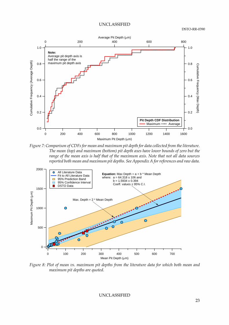
UNCLASSIFIED DSTO-RR-0390
UNCLASSIFIED 23
1.0
0.8
0.6
0.4
0.2
0.0
Cum
ula
tive Frequ
ency (M
ax D
epth)
1.0
0.8
0.6
0.4
0.2
0.0
Cu
mul
ativ
e F
req
uenc
y (A
vera
ge
De
pth)
8006004002000Average Pit Depth (m)
16001400120010008006004002000
Maximum Pit Depth (m)
Pit Depth CDF Distribution Maximum Average
Note:Average pit depth axis ishalf the range of themaximum pit depth axis
Figure 7: Comparison of CDFs for mean and maximum pit depth for data collected from the literature.
The mean (top) and maximum (bottom) pit depth axes have lower bounds of zero but the range of the mean axis is half that of the maximum axis. Note that not all data sources reported both mean and maximum pit depths. See Appendix A for references and raw data.
2000
1500
1000
500
0
Max
imum
Pit
Dep
th (m
)
7006005004003002001000
Mean Pit Depth (m)
All Literature Data Fit to All Literature Data 95% Prediction Band 95% Confidence Interval DSTO Data
Equation: Max Depth = a + b * Mean Depthwhere: a = 64.318 ± 106 and
b = 1.5934 ± 0.394Coeff. values ± 95% C.I.
Max. Depth = 2 * Mean Depth
Figure 8: Plot of mean vs. maximum pit depths from the literature data for which both mean and
maximum pit depths are quoted.
UNCLASSIFIED DSTO-RR-0390
UNCLASSIFIED 24
3. Experimental Material23
3.1 Introduction
The aluminium alloy 7010-T7651 was used for the research described in this report. The specimens tested in this research were machined from a rolled slab of this material purchased during the SICAS project. This alloy is the principal alloy of the BAE SYSTEMS Hawk Mk 127, which is used by the RAAF as a ‘Lead-in Fighter Trainer’. RAAF fighter pilots are trained on the Hawk before moving on to the F/A-18 Hornet. This section describes the composition and microstructure of this alloy. The microstructure is described by statistical descriptions of its grain and inclusion size distributions. These descriptions are limited to the details needed to develop the models described in this report. The material was sourced from two billets of rolled 7010-T7651 which were manufactured by Pechiney UK. They were purchased by BAE SYSTEMS UK24 through Apollo Metals25, who were BAE SYSTEMS primary supplier of materials at that time26. The billets was processed by Apollo Metals to produce two plates of 3014 mm length (L - rolling direction), 1304 mm width (T – long transverse) and 60 mm thickness (S – short transverse). These plates were then machined by Gretones27, a UK machinist, to produce tensile, fatigue life and fatigue crack growth specimens. 3.2 Composition
The composition of the 7010-T7651 aluminium alloy was determined during the SICAS project by dissolving four approximately 10 x 10 x 10 mm samples of the alloy in mixed acids followed by inductively coupled plasma analysis of the resultant solution (ICP-AES). The results of this analysis, Table 1, show that the alloy falls within the compositions range allowed for 7010 for all of the elements tested [105]. This table also lists the compositional data reported on the certificate of conformity that came with the material [106].
23 Much of the material in this section derives from Chapter 4 of [3]. It is reproduced here for the reader’s convenience and because [3] is not publicly available. 24 BAE SYSTEMS, Samlesbury Aerodrome, Balderstone, Lancashire, BB2 7LF, United Kingdom 25 Apollo Metals was acquired by Thyssen Krupp in 2007 and is now ThyssenKrupp Aerospace UK Ltd. Redfern Road, Tyseley, B11 2BH Birmingham, West Midlands, United Kingdom 26 The authors are not aware if Thyssen Krupp, who acquired Apollo Metals in 2007, are still the principal supplier of aluminium alloys for BAE SYSTEMS. 27 Gretones, Scafell Road, Lytham-St Anne, Lancashire, FY8 3EB

UNCLASSIFIED DSTO-RR-0390
UNCLASSIFIED 25
Table 1: Mean chemical composition of 7010-T7651 in weight percentages measured from four specimens compared with the specification for the alloy (‘Specification’) and the composition cited in the material’s certificate of conformity (‘Certificate’). All measured values are within the specified range.
Element % Zn % Cu % Mg % Zr % Fe % Cr % Mn % Si % Ti
Measured 6.0 1.7 2.1 0.11 0.09 0.006 0.015 0.074 0.025
Certificate 6.00 1.57 2.21 0.11 0.08 0.006 0.01 0.05 0.02
Specification 5.7-6.7 1.5-2.0 2.1-2.6 0.1-0.16 0-0.15 0-0.05 0-0.1 0-0.12 0-0.06
3.3 Microstructure
Figure 9 shows the microstructure of this material as an isometric cube, which shows the material’s three principal planes (LT, LS and TS). The material in this image had been polished to a sub-micron finish and etched using Keller’s reagent to reveal its grain structure. The pancaked microstructure observed in this figure is typical of a rolled, unrecrystallised aluminium alloy. The mean grain sizes were 730, 170 and 40 m in the L, T and S directions respectively. These sizes were measured using the mean lineal intercept method described in ASTM E112-10 [107].
L
T
S
Figure 9: Three-plane micrograph of etched 7010-T7651 showing the grain boundaries and inclusions.
Scale bars indicate 50 m.
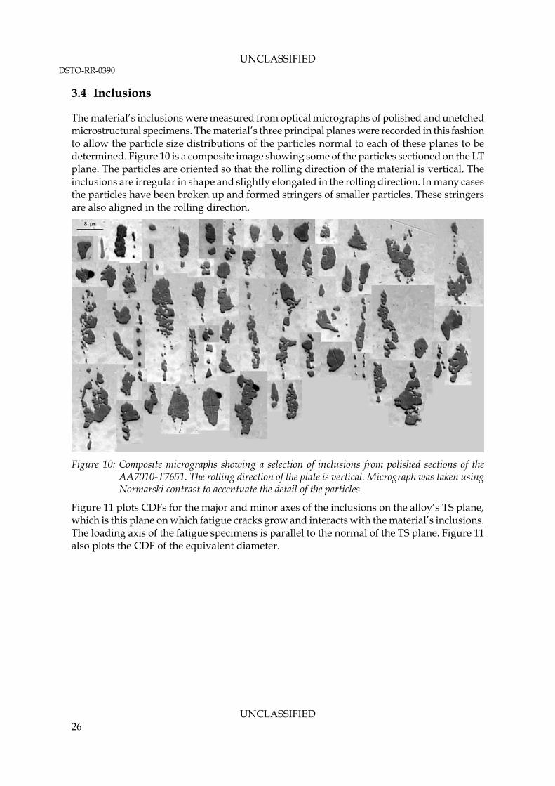
UNCLASSIFIED DSTO-RR-0390
UNCLASSIFIED 26
3.4 Inclusions
The material’s inclusions were measured from optical micrographs of polished and unetched microstructural specimens. The material’s three principal planes were recorded in this fashion to allow the particle size distributions of the particles normal to each of these planes to be determined. Figure 10 is a composite image showing some of the particles sectioned on the LT plane. The particles are oriented so that the rolling direction of the material is vertical. The inclusions are irregular in shape and slightly elongated in the rolling direction. In many cases the particles have been broken up and formed stringers of smaller particles. These stringers are also aligned in the rolling direction.
Figure 10: Composite micrographs showing a selection of inclusions from polished sections of the
AA7010-T7651. The rolling direction of the plate is vertical. Micrograph was taken using Normarski contrast to accentuate the detail of the particles.
Figure 11 plots CDFs for the major and minor axes of the inclusions on the alloy’s TS plane, which is this plane on which fatigue cracks grow and interacts with the material’s inclusions. The loading axis of the fatigue specimens is parallel to the normal of the TS plane. Figure 11 also plots the CDF of the equivalent diameter.
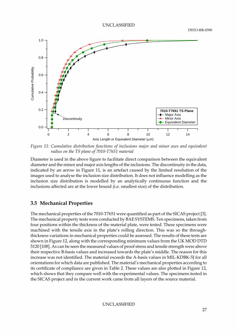
UNCLASSIFIED DSTO-RR-0390
UNCLASSIFIED 27
1.0
0.8
0.6
0.4
0.2
0.0
Cum
ulat
ive P
roba
bilit
y
14121086420
Axis Length or Equivalent Diameter (m)
7010-T7651 TS Plane Major Axis Minor Axis Equivalent Diameter
Discontinuity
Figure 11: Cumulative distribution functions of inclusions major and minor axes and equivalent
radius on the TS plane of 7010-T7651 material
Diameter is used in the above figure to facilitate direct comparison between the equivalent diameter and the minor and major axis lengths of the inclusions. The discontinuity in the data, indicated by an arrow in Figure 11, is an artefact caused by the limited resolution of the images used to analyse the inclusion size distribution. It does not influence modelling as the inclusion size distribution is modelled by an analytically continuous function and the inclusions affected are at the lower bound (i.e. smallest size) of the distribution. 3.5 Mechanical Properties
The mechanical properties of the 7010-T7651 were quantified as part of the SICAS project [3]. The mechanical property tests were conducted by BAE SYSTEMS. Ten specimens, taken from four positions within the thickness of the material plate, were tested. These specimens were machined with the tensile axis in the plate’s rolling direction. This was so the through-thickness variations in mechanical properties could be assessed. The results of these tests are shown in Figure 12, along with the corresponding minimum values from the UK MOD DTD 5120 [108]. As can be seen the measured values of proof stress and tensile strength were above their respective B-basis values and increased towards the plate’s middle. The reason for this increase was not identified. The material exceeds the A-basis values in MIL-KDBK-5J for all orientations for which data are published. The material’s mechanical properties according to its certificate of compliance are given in Table 2. These values are also plotted in Figure 12, which shows that they compare well with the experimental values. The specimens tested in the SICAS project and in the current work came from all layers of the source material.

UNCLASSIFIED DSTO-RR-0390
UNCLASSIFIED 28
Table 2: Mechanical properties of 7010-T7651 alloy as stated in its certificate of compliance. TS and 0.2 values in brackets are authoritative value in ksi. The values not in brackets are converted to MPa and are not authoritative.
Slab Direction TS (MPa)
0.2 (MPa)
f (%)
KIC (MPam)
L 528 477 15 —
ST 522 449 7.6 — 1
TL 536 481 11 —
L 542 490 13 40.2
ST 518 446 7.5 — 2
TL 538 483 11 33.7
L 517 (75) 448 (65) 8 —
ST 490 (71) 407 (59) 2.5 — MIL-HDBK-5J
A-Basis (2.5") TL — — — —
560
540
520
500
480
460
440
Str
ess
(MP
a)
6050403020100Specimen Location Depth (mm from top surface)
7010-T7651 Mechanical Properties
0.2% Proof Stress Tensile Strength
B-Basis 0.2% Proof Stress (453 MPa)
B-Basis Tensile Strength (510 MPa)
Slab 1: 0.2% Proof Stress (477 MPa)
Slab 2: 0.2% Proof Stress (490 MPa)
Slab 1: Tensile Strength (528 MPa)
Slab 2: Tensile Strength (542 MPa)
Figure 12: 0.2% Proof Stress and Tensile Strength of 7010-T7651 material in the L-direction as a
function of specimen location depth within the original material slab compared to the nominal B-basis values for this alloy and the mechanical property data from the material’s certificate of compliance.
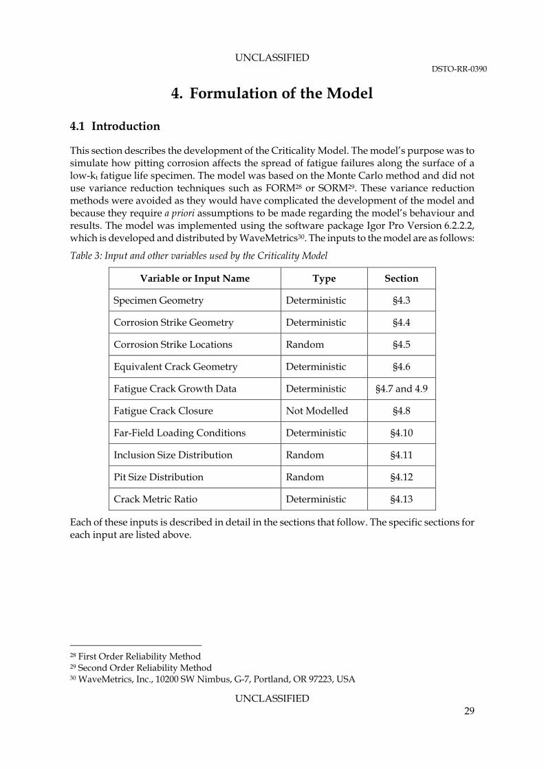
UNCLASSIFIED DSTO-RR-0390
UNCLASSIFIED 29
4. Formulation of the Model
4.1 Introduction
This section describes the development of the Criticality Model. The model’s purpose was to simulate how pitting corrosion affects the spread of fatigue failures along the surface of a low-kt fatigue life specimen. The model was based on the Monte Carlo method and did not use variance reduction techniques such as FORM28 or SORM29. These variance reduction methods were avoided as they would have complicated the development of the model and because they require a priori assumptions to be made regarding the model’s behaviour and results. The model was implemented using the software package Igor Pro Version 6.2.2.2, which is developed and distributed by WaveMetrics30. The inputs to the model are as follows:
Table 3: Input and other variables used by the Criticality Model
Variable or Input Name Type Section
Specimen Geometry Deterministic §4.3
Corrosion Strike Geometry Deterministic §4.4
Corrosion Strike Locations Random §4.5
Equivalent Crack Geometry Deterministic §4.6
Fatigue Crack Growth Data Deterministic §4.7 and 4.9
Fatigue Crack Closure Not Modelled §4.8
Far-Field Loading Conditions Deterministic §4.10
Inclusion Size Distribution Random §4.11
Pit Size Distribution Random §4.12
Crack Metric Ratio Deterministic §4.13
Each of these inputs is described in detail in the sections that follow. The specific sections for each input are listed above.
28 First Order Reliability Method 29 Second Order Reliability Method 30 WaveMetrics, Inc., 10200 SW Nimbus, G-7, Portland, OR 97223, USA

UNCLASSIFIED DSTO-RR-0390
UNCLASSIFIED 30
4.2 Algorithm
The Criticality Model is a weakest link or series model, in that failure occurs when any single element fails. Therefore the life of the model is determined by the life of the element that fails first. In this context, a model element is a surface inclusion or corrosion pit and its associated fatigue crack. Figure 13is a flowchart of the algorithm of the Criticality Model. This section will describe the model’s algorithm and its rationale. Appendix C contains a mathematical description of the model and its source code can be found in Appendix D. The Criticality Model is based upon a Monte Carlo simulation. The Monte Carlo method can be used to numerically integrate equations that cannot be integrated analytically. It is particularly useful for the integration of equations with many variables. The current model estimates the probability of failure due to a corrosion pit at a given location on the specimen. It is therefore calculating a definite integral which is based on the distributions of pit size and location and the stress gradient of the specimen being modelled. 4.2.1 Step 1: Start of Program
Starting a simulation run of the Criticality Model invokes two procedures in series. The first updates the pit and inclusion size distributions. This ensures that these distributions are updated before the main loop of the model start executing. The second procedure is the model’s main loop, which controls the its overall execution. The model ends when the main loop of the model (Steps 6 to 17) is complete and the results have been output (Step 18). 4.2.2 Steps 2 to 5: Array and Variable Initialisation
Steps 2 to 5 of the algorithm prepare the arrays31 and variables needed by the model. The major arrays created in Main are the result storage arrays. These store the location, size, local stress, CMR, fatigue life and type for each critical defect. A critical defect is the defect with the shortest fatigue life each of the model’s iterations. At this stage all of the elements in these arrays are declared equal to NaN32. They are not given values until the main loop of the program (§4.2.3) where they are used to record characteristics of the critical defect for each iteration of the model. Once the storage arrays have been created the program determines how many inclusions and pits are to be modelled in each iteration of the model. The use of extreme value statistics means that it is only necessary to model the largest pit or inclusion in a given area33. This greatly reduces the computational demands of the model. 31 Igor Pro stores data in structures called that it calls ‘waves’. This is because Igor Pro was originally intended for the digital signal processing. These waves resembles arrays except that they are time series with a defined time increment between each element of the wave. In the current model this time increment was not used and the waves were treated as if they were simple arrays. 32 NaN = Not a Number. This is a special value used in numerical programming to indicate that a variable or an element of an array is not a number and cannot be used for calculation. Any calculation that involves a NaN value will itself return a NaN value, which is an error condition. 33 It should be noted that extreme value distributions may not accurately describe the size of all of the corrosion pits on a specimen’s surface. Trueman [109] notes that there are often two types of pits on the corroded surfaces of aluminium alloys which he denoted as ‘stable’ and ‘meta-stable’ pits. These have

UNCLASSIFIED DSTO-RR-0390
UNCLASSIFIED 31
The program then creates two arrays which store the characteristic data of the pits and inclusions for each iteration of the model. One of these pits or inclusions will be the critical pit for a given iteration. At this stage all of the elements in these arrays are set to NaN. They are not given values until the main loop of the program. This ensures that each iteration of the model is different. Finally, if the location of the corrosion strike is fixed, the program calculates the start and end points of the corrosion strike on the specimen. 4.2.3 Steps 6 to 17: Main Loop
These steps are the main loop of the program. Each iteration of this loop simulates a fatigue test of a single fatigue specimen. The loop ends when the number of iterations set by the user is reached. In Step 7 a random set of inclusions and pits are created based on the inverse defect size distributions for each kind of defect. In Steps 8 and 9 the location of the centre of the corrosion strike is determined. If the corrosion strike is randomly located the centre of the corrosion strike is calculated separately for each iteration. Otherwise, the centre of the corrosion strike is set to the user selected value. The pits in this corrosion strike are generated in Step 11 assuming that the user has asked for corrosion pits to be modelled. If the user has not asked for corrosion pits then no pits are created. The option to not model corrosion was included so that the model could predict the fatigue lives and failure locations of uncorroded specimens. The pit and inclusion with the shortest fatigue lives for their defect type are identified in Steps 12 and 13 respectively. These fatigue life minima are then compared in Step 14to determine if the specimen failed due to a corrosion pit or an inclusion. If failure was due to an inclusion then the characteristics of the critical inclusion are recorded in the results array in Step 15. Conversely, if failure was due to a corrosion pit then the characteristics of the critical pit are recorded in Step 16. The last step in the main loop is Step 17. If the set number of iterations has been completed then the main loop terminates and execution moves onto Step 18. Otherwise, the program returns to Step 6 to repeat the program’s main loop.
different electrochemical growth mechanisms and therefore different size distributions. Their combined size distribution is typically bimodal. However, in fatigue it is typically the larger defects that control the fatigue life of a component or material. Extreme value distributions describe the size of the largest pits well.

UNCLASSIFIED DSTO-RR-0390
UNCLASSIFIED 32
1. Start Main
2. Initialise arrays and variables
3. Calculate number of intrinsic
defects and pits
4. Create pit and intrinsic defect
arrays
6. For loop (icount = 0 to
repeatsstep 1)
7. function MakeDefects(inclusions)
8 Random corrosion centre?
9. Calculate random start and end of corrosion
area
5. Calculate startand end of fixed corrosion area
Y
10. Pitting present?
No
Y
11. functionMakeDefects
(corrosion pits)
12. Find minimum
corrosion pit life
13. Find minimum intrinsic
defect life
A
A
14. Pittingfatigue life < inclusion
fatigue life
16. Record position, size,
stress and life of corrosion pit in
results array
B
15. Record position, size,
stress and life of inclusion in results array
17. For loop complete?
BNo
18. Update results histograms
Yes
19. End Main
No
N Y
Figure 13: Algorithm of the Criticality Model. The model’s main loop is shown in orange while the
sections in blue are executed once.

UNCLASSIFIED DSTO-RR-0390
UNCLASSIFIED 33
4.2.4 Step 18: Calculation of Final Results
In Step 18, the model’s final results are calculated and plotted. The results generated are:
1. Radius of the critical defect
2. Position of the critical defect along the specimen’s centreline
3. Stress at the critical defect
4. Radius of the critical defect adjusted by the CMR
5. The fatigue life of the critical defect A set of these five outputs is produced for each iteration of the model. These arrays can then be analysed and plotted for further analysis as required by the model’s user. 4.2.5 Step 19: Program Termination
This step terminates the execution of the model. 4.3 Specimen Geometry
The specimen geometry used in this model (Figure 14) was used in the SICAS project [3, 4]. It is a 420 mm long low-kt fatigue specimen with a rectangular cross section which has slightly rounded corners. The long axis of the specimen is parallel to the rolling direction of the source material plate. This specimen geometry, with the exception of the rounded corners, conforms to the dimensional requirements of ASTM 466-07 [2]. The rounded corners were added to the geometry to discourage the initiation and growth of fatigue cracks from the corners of uncorroded specimens. The corners of the uncorroded specimens were also shot peened to further discourage corner cracking.
7 5
420
R200
194
25
8
R1.5
Figure 14: Specimen geometry used for the Criticality Model. This was the standard fatigue specimen
used in the SICAS project. The horizontal dash-dot line along the specimen’s length is both the specimen’s centreline and its idealised loading axis. This axis is along the L-axis of the source material while the specimens face is in the LT plane. All dimensions are in millimetres.
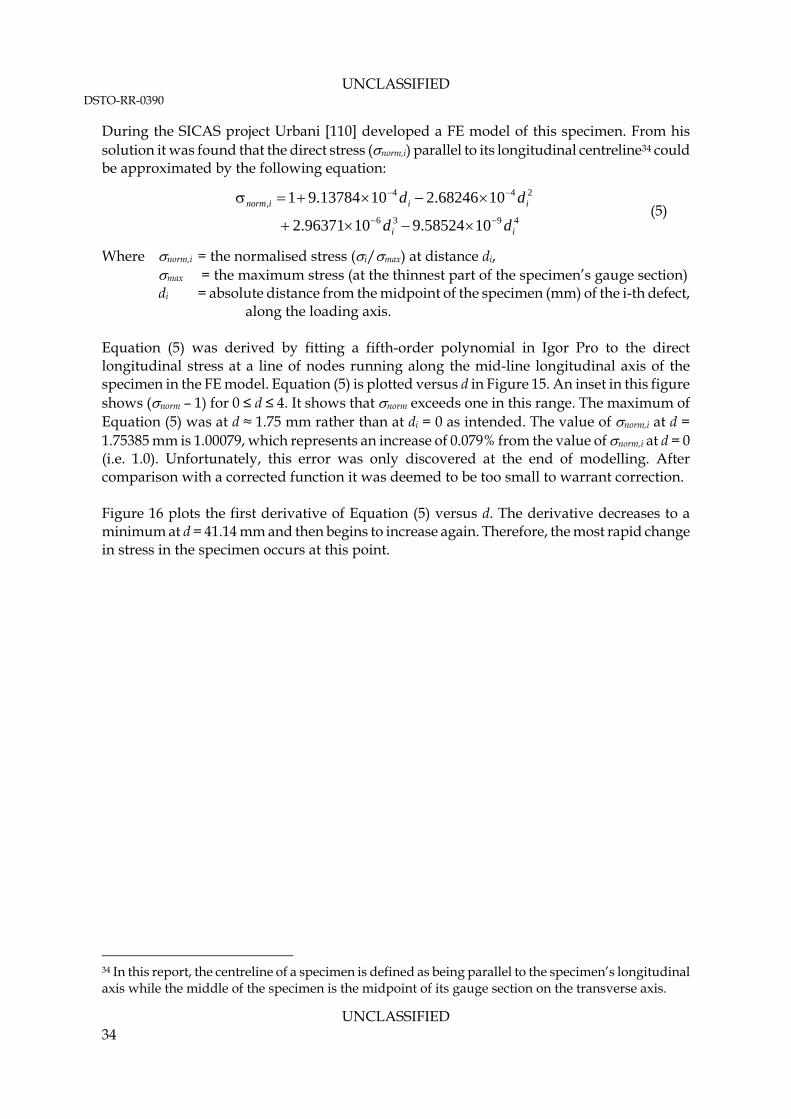
UNCLASSIFIED DSTO-RR-0390
UNCLASSIFIED 34
During the SICAS project Urbani [110] developed a FE model of this specimen. From his solution it was found that the direct stress (norm,i) parallel to its longitudinal centreline34 could be approximated by the following equation:
4936
244,
1058524.91096371.2
1068246.21013784.91
ii
iiinorm
dd
dd
(5)
Where norm,i = the normalised stress (i/max) at distance di, max = the maximum stress (at the thinnest part of the specimen’s gauge section) di = absolute distance from the midpoint of the specimen (mm) of the i-th defect, along the loading axis. Equation (5) was derived by fitting a fifth-order polynomial in Igor Pro to the direct longitudinal stress at a line of nodes running along the mid-line longitudinal axis of the specimen in the FE model. Equation (5) is plotted versus d in Figure 15. An inset in this figure shows (norm – 1) for 0 ≤ d ≤ 4. It shows that norm exceeds one in this range. The maximum of Equation (5) was at d ≈ 1.75 mm rather than at di = 0 as intended. The value of norm,i at d = 1.75385 mm is 1.00079, which represents an increase of 0.079% from the value of norm,i at d = 0 (i.e. 1.0). Unfortunately, this error was only discovered at the end of modelling. After comparison with a corrected function it was deemed to be too small to warrant correction. Figure 16 plots the first derivative of Equation (5) versus d. The derivative decreases to a minimum at d = 41.14 mm and then begins to increase again. Therefore, the most rapid change in stress in the specimen occurs at this point.
34 In this report, the centreline of a specimen is defined as being parallel to the specimen’s longitudinal axis while the middle of the specimen is the midpoint of its gauge section on the transverse axis.
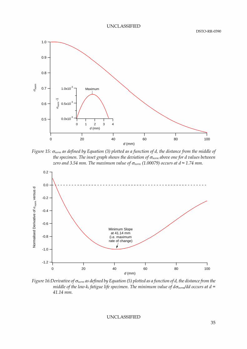
UNCLASSIFIED DSTO-RR-0390
UNCLASSIFIED 35
1.0
0.9
0.8
0.7
0.6
0.5
nor
m
100806040200d (mm)
1.0x10⁻³
0.5x10⁻³
0.0x10⁻³
no
rm -
1
43210d (mm)
Maximum
Figure 15: norm as defined by Equation (3) plotted as a function of d, the distance from the middle of the specimen. The inset graph shows the deviation of norm above one for d values between zero and 3.54 mm. The maximum value of norm (1.00079) occurs at d ≈ 1.74 mm.
-1.2
-1.0
-0.8
-0.6
-0.4
-0.2
0.0
0.2
Nor
ma
lise
d D
eriv
ativ
e o
f n
orm
ve
rsus
d
100806040200d (mm)
Minimum Slopeat 41.14 mm
(i.e. maximumrate of change)
Figure 16:Derivative of norm as defined by Equation (5) plotted as a function of d, the distance from the middle of the low-kt fatigue life specimen. The minimum value of dnorm/dd occurs at d = 41.14 mm.
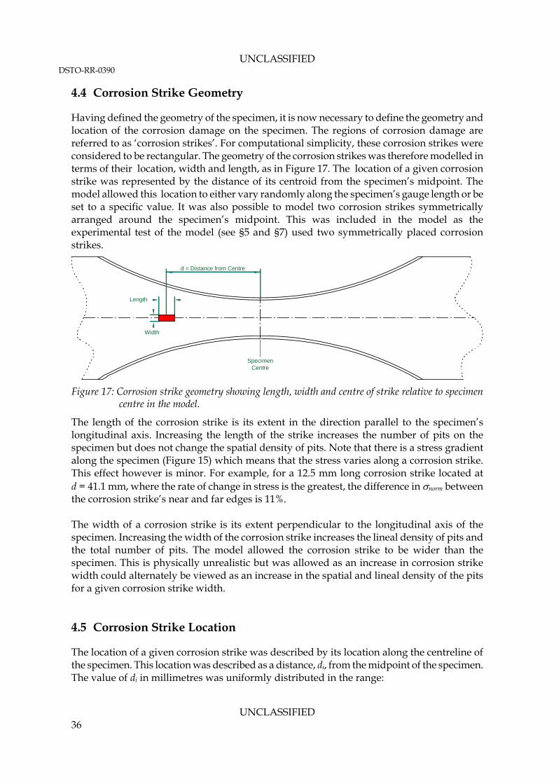
UNCLASSIFIED DSTO-RR-0390
UNCLASSIFIED 36
4.4 Corrosion Strike Geometry
Having defined the geometry of the specimen, it is now necessary to define the geometry and location of the corrosion damage on the specimen. The regions of corrosion damage are referred to as ‘corrosion strikes’. For computational simplicity, these corrosion strikes were considered to be rectangular. The geometry of the corrosion strikes was therefore modelled in terms of their location, width and length, as in Figure 17. The location of a given corrosion strike was represented by the distance of its centroid from the specimen’s midpoint. The model allowed this location to either vary randomly along the specimen’s gauge length or be set to a specific value. It was also possible to model two corrosion strikes symmetrically arranged around the specimen’s midpoint. This was included in the model as the experimental test of the model (see §5 and §7) used two symmetrically placed corrosion strikes.
d = Distance from Centre
Length
Width
SpecimenCentre
Figure 17: Corrosion strike geometry showing length, width and centre of strike relative to specimen
centre in the model.
The length of the corrosion strike is its extent in the direction parallel to the specimen’s longitudinal axis. Increasing the length of the strike increases the number of pits on the specimen but does not change the spatial density of pits. Note that there is a stress gradient along the specimen (Figure 15) which means that the stress varies along a corrosion strike. This effect however is minor. For example, for a 12.5 mm long corrosion strike located at d = 41.1 mm, where the rate of change in stress is the greatest, the difference in norm between the corrosion strike’s near and far edges is 11%. The width of a corrosion strike is its extent perpendicular to the longitudinal axis of the specimen. Increasing the width of the corrosion strike increases the lineal density of pits and the total number of pits. The model allowed the corrosion strike to be wider than the specimen. This is physically unrealistic but was allowed as an increase in corrosion strike width could alternately be viewed as an increase in the spatial and lineal density of the pits for a given corrosion strike width. 4.5 Corrosion Strike Location
The location of a given corrosion strike was described by its location along the centreline of the specimen. This location was described as a distance, di, from the midpoint of the specimen. The value of di in millimetres was uniformly distributed in the range:

UNCLASSIFIED DSTO-RR-0390
UNCLASSIFIED 37
2
982
98 corrosioni
corrosion ld
l (6)
where lcorrosion = the length of the corrosion strike. Note that the corrosion pits are contained within these corrosion strikes. This is typical of what is seen in in-service aircraft. That is, localised damage to the corrosion protection scheme leads to localised corrosion damage. The location of a corrosion pit within a corrosion strike, dpit, is distributed uniformly within the range given by:
22
corrosionipit
corrosioni
ldd
ld (7)
If there are multiple corrosion pits within a corrosion strike then each is located independently. 4.6 Equivalent Crack Geometry
The Criticality Model uses the specimen and crack geometry used in the SICAS project [3, 4]. Given that the corrosion pits in that project were restricted to one surface of the fatigue specimen the Criticality Model uses a centred semi-circular surface crack to represent them, Figure 18. The surface crack was on the wide face of the specimens. Note that specimen becomes wider as the equivalent crack moves away from the centre of the specimen. A semi-circular crack was used in preference to a semi-elliptical crack as its size could be described by a single quantity, its radius. Fatigue crack growth modelling was conducted using AFGROW [38] using the -solutions in that program, which were developed by Raju and Newman [66]. In contrast to many weakest-link models of fatigue and fracture which simulate the initiation of cracks from surface and internal defects, the Criticality Model concentrates solely on surface initiation mechanisms. This was considered reasonable as none of the approximately 350 fatigue specimens tested in the SICAS project failed due to fatigue cracks initiated from sub-surface defects.
Semi-Circular Crack8
25
Figure 18: Centred semi-circular crack model used to represent corrosion pits in the Criticality Model. All dimensions are in millimetres.
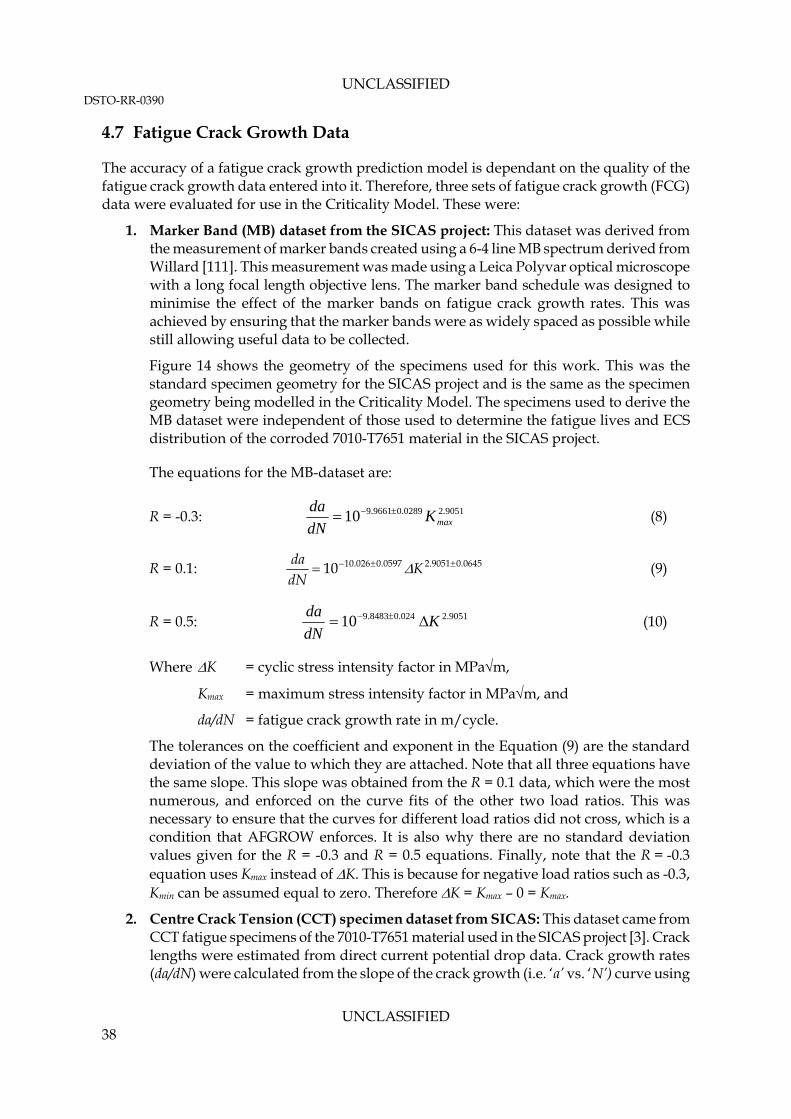
UNCLASSIFIED DSTO-RR-0390
UNCLASSIFIED 38
4.7 Fatigue Crack Growth Data
The accuracy of a fatigue crack growth prediction model is dependant on the quality of the fatigue crack growth data entered into it. Therefore, three sets of fatigue crack growth (FCG) data were evaluated for use in the Criticality Model. These were:
1. Marker Band (MB) dataset from the SICAS project: This dataset was derived from the measurement of marker bands created using a 6-4 line MB spectrum derived from Willard [111]. This measurement was made using a Leica Polyvar optical microscope with a long focal length objective lens. The marker band schedule was designed to minimise the effect of the marker bands on fatigue crack growth rates. This was achieved by ensuring that the marker bands were as widely spaced as possible while still allowing useful data to be collected.
Figure 14 shows the geometry of the specimens used for this work. This was the standard specimen geometry for the SICAS project and is the same as the specimen geometry being modelled in the Criticality Model. The specimens used to derive the MB dataset were independent of those used to determine the fatigue lives and ECS distribution of the corroded 7010-T7651 material in the SICAS project.
The equations for the MB-dataset are:
R = -0.3: 9051.20289.09661.910 maxKdN
da (8)
R = 0.1: 0645.09051.20597.0026.1010 KdNda (9)
R = 0.5: 9051.2024.08483.910 KdN
da (10)
Where K = cyclic stress intensity factor in MPam,
Kmax = maximum stress intensity factor in MPam, and
da/dN = fatigue crack growth rate in m/cycle.
The tolerances on the coefficient and exponent in the Equation (9) are the standard deviation of the value to which they are attached. Note that all three equations have the same slope. This slope was obtained from the R = 0.1 data, which were the most numerous, and enforced on the curve fits of the other two load ratios. This was necessary to ensure that the curves for different load ratios did not cross, which is a condition that AFGROW enforces. It is also why there are no standard deviation values given for the R = -0.3 and R = 0.5 equations. Finally, note that the R = -0.3 equation uses Kmax instead of K. This is because for negative load ratios such as -0.3, Kmin can be assumed equal to zero. Therefore K = Kmax – 0 = Kmax.
2. Centre Crack Tension (CCT) specimen dataset from SICAS: This dataset came from CCT fatigue specimens of the 7010-T7651 material used in the SICAS project [3]. Crack lengths were estimated from direct current potential drop data. Crack growth rates (da/dN) were calculated from the slope of the crack growth (i.e. ‘a’ vs. ‘N’) curve using
UNCLASSIFIED DSTO-RR-0390
UNCLASSIFIED 39
the seven point secant method. No measurements of crack closure were made during fatigue testing.
3. 7010-T7 FCG NASGRO model from the AFGROW material database: This is a standard fatigue crack growth dataset included in AFGROW [38]. It comes originally from the NASGRO fatigue crack prediction code [36].
These data are compared in Figure 19 at a load ratio, R, of 0.1 35. The MB and CCT datasets are similar while the NASGRO dataset has significantly higher growth rates over its entire K range. At 10 MPa√m, the NASGRO model predicts a growth rate that is 50 times faster than that predicted by the MB dataset and 20 times faster than predicted by the CCT dataset. However, the NASGRO datasets has a fatigue threshold and a near-fast fracture region, which both the MB and FCC datasets lack.
The lack of a threshold in the MB and CCT datasets was considered acceptable as no fatigue threshold effects were observed in the collection of the MB data. The lack of a near-fast fracture region in the MB and CCT datasets was considered unimportant as fracture toughness strongly affects the crack length at fast fracture but has only a minimal affect on fatigue life due to the speed of crack growth as Kmax approaches the material’s fracture toughness.
10-11
10-10
10-9
10-8
10-7
10-6
10-5
10-4
10-3
10-2
10-1
100
da/d
n (
m/c
ycle
)
12 3 4 5 6 7 8 9
102 3 4 5 6 7 8 9
1002 3
K (MPam)
NASGRO Marker Band CCT
Figure 19: Comparison of Marker Band and CCT fatigue crack growth data from the SICAS project
with the NASGRO data for 7010-T73651 from AFGROW’s database of NASGRO parameters [38].
35 Appendix E contains a table of the complete MB fatigue dataset.
UNCLASSIFIED DSTO-RR-0390
UNCLASSIFIED 40
4.8 Fatigue Crack Closure
Various fatigue crack closure mechanisms have been proposed to explain crack retardation and acceleration effects under variable amplitude loading [41]. In particular, the fatigue crack prediction code FASTRAN uses plasticity induced crack closure to model fatigue crack growth under variable amplitude loading conditions. No attempt was made to use fatigue crack closure in the Criticality Model for three reasons. Firstly, the model only considers fatigue under constant amplitude conditions at the same R value at which the fatigue crack growth data were collected. Variable amplitude loading is not modelled. Secondly, in the case of the MB dataset, the fatigue crack growth data were collected from specimens of the same geometry as being modelled. Finally, the cracks being modelled are at most 8 mm deep (the thickness of the specimens) and would typically be much less than this for most of the specimen’s fatigue life, i.e. around 1-2 mm. Cracks of this size are typically considered to be ‘physically small’ [41], which means they lack the crack wake needed for crack closure effects to become significant. 4.9 Fatigue Life Lookup Table
The three datasets in the previous section were used to create, using AFGROW [38], lookup tables of estimated fatigue life as a function of defect size and local stress. That is:
RrN iif ,,g max, (11)
where Nf,i = fatigue cycles to failure of the i-th defect, g = fatigue life calculation function, ri = defect( i.e. pit or inclusion) radius of the i-th defect,
R = load ratio =max
min
,
min = remote minimum stress, and max = remote maximum stress. Note that the fatigue life calculation function, g, was different for each of the three fatigue crack growth datasets. In addition, it was assumed that the small size of the equivalent cracks compared to the specimen’s size and the shallow stress gradient of the specimen meant that it was acceptable to use the stress calculated using Equation (5) as the remote stress. Finally, the scatter in the fatigue crack growth rate data, as represented by the standard deviations given in Equation (9), were not modelled. Therefore the fatigue life lookup table was deterministic in that a given combination of defect size and remote stress would always give the same value of predicted fatigue life. As stated in §4.6, the defects were assumed to be semi-circular and their size was therefore characterised using their radius. A study of the effect of initial aspect ratio on predicted fatigue life was made using AFGROW and the MB dataset at max = 380 MPa and R = 0.1, Figure 20. It found that semi-circular initial cracks gave the longest predicted fatigue lives though the effect was only modest. Over a range of pit aspect ratios between 0.25 and 4 the change in predicted life was less than 5%.
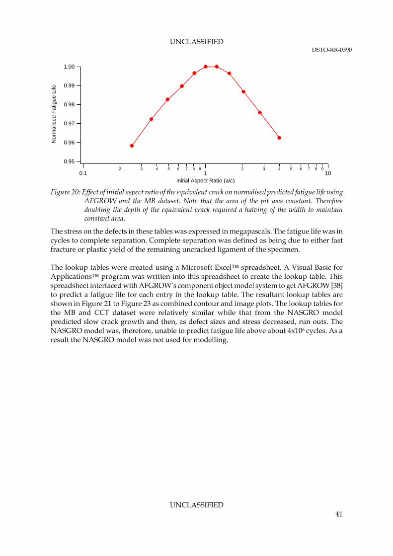
UNCLASSIFIED DSTO-RR-0390
UNCLASSIFIED 41
1.00
0.99
0.98
0.97
0.96
0.95
Nor
mal
ised
Fat
igue
Life
0.12 3 4 5 6 7 8 9
12 3 4 5 6 7 8 9
10Initial Aspect Ratio (a/c)
Figure 20: Effect of initial aspect ratio of the equivalent crack on normalised predicted fatigue life using AFGROW and the MB dataset. Note that the area of the pit was constant. Therefore doubling the depth of the equivalent crack required a halving of the width to maintain constant area.
The stress on the defects in these tables was expressed in megapascals. The fatigue life was in cycles to complete separation. Complete separation was defined as being due to either fast fracture or plastic yield of the remaining uncracked ligament of the specimen. The lookup tables were created using a Microsoft Excel™ spreadsheet. A Visual Basic for Applications™ program was written into this spreadsheet to create the lookup table. This spreadsheet interfaced with AFGROW’s component object model system to get AFGROW [38] to predict a fatigue life for each entry in the lookup table. The resultant lookup tables are shown in Figure 21 to Figure 23 as combined contour and image plots. The lookup tables for the MB and CCT dataset were relatively similar while that from the NASGRO model predicted slow crack growth and then, as defect sizes and stress decreased, run outs. The NASGRO model was, therefore, unable to predict fatigue life above about 4x10⁶ cycles. As a result the NASGRO model was not used for modelling.
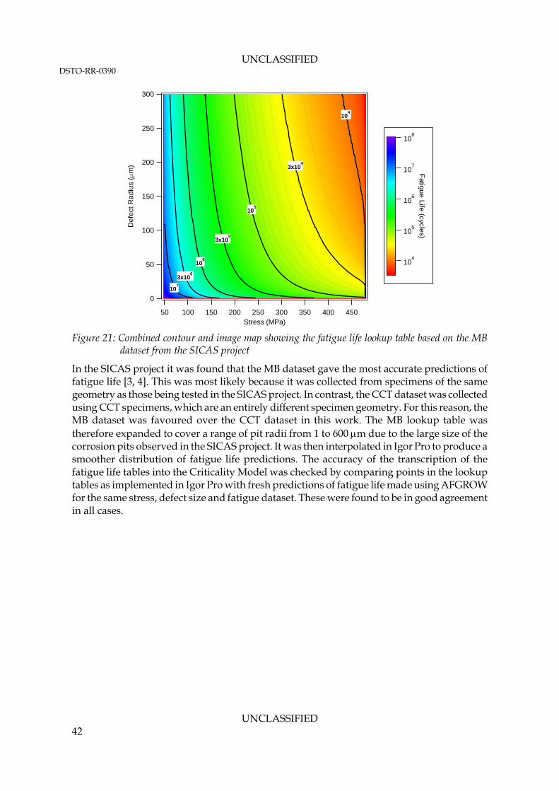
UNCLASSIFIED DSTO-RR-0390
UNCLASSIFIED 42
300
250
200
150
100
50
0
De
fect
Ra
diu
s (
m)
45040035030025020015010050Stress (MPa)
107
3x10⁶
106
3x10⁵
105
3x10⁴
104
104
105
106
107
108
Fatig
ue
Life
(cycles)
Figure 21: Combined contour and image map showing the fatigue life lookup table based on the MB
dataset from the SICAS project
In the SICAS project it was found that the MB dataset gave the most accurate predictions of fatigue life [3, 4]. This was most likely because it was collected from specimens of the same geometry as those being tested in the SICAS project. In contrast, the CCT dataset was collected using CCT specimens, which are an entirely different specimen geometry. For this reason, the MB dataset was favoured over the CCT dataset in this work. The MB lookup table was therefore expanded to cover a range of pit radii from 1 to 600 m due to the large size of the corrosion pits observed in the SICAS project. It was then interpolated in Igor Pro to produce a smoother distribution of fatigue life predictions. The accuracy of the transcription of the fatigue life tables into the Criticality Model was checked by comparing points in the lookup tables as implemented in Igor Pro with fresh predictions of fatigue life made using AFGROW for the same stress, defect size and fatigue dataset. These were found to be in good agreement in all cases.
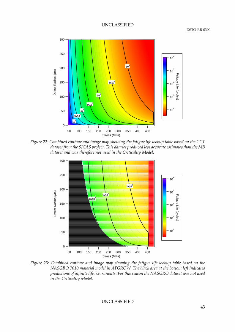
UNCLASSIFIED DSTO-RR-0390
UNCLASSIFIED 43
300
250
200
150
100
50
0
De
fect
Ra
diu
s (
m)
45040035030025020015010050Stress (MPa)
3x10⁶
106
105
3x10⁴
104
104
105
106
107
108
Fatig
ue Life
(cycles)
3x10⁵
107
Figure 22: Combined contour and image map showing the fatigue life lookup table based on the CCT
dataset from the SICAS project. This dataset produced less accurate estimates than the MB dataset and was therefore not used in the Criticality Model.
300
250
200
150
100
50
0
De
fect
Ra
diu
s (
m)
45040035030025020015010050Stress (MPa)
3x10⁵
1x10⁵
3x10⁴
104
105
106
107
108
Fatig
ue
Life
(cycles)
Figure 23: Combined contour and image map showing the fatigue life lookup table based on the
NASGRO 7010 material model in AFGROW. The black area at the bottom left indicates predictions of infinite life, i.e. runouts. For this reason the NASGRO dataset was not used in the Criticality Model.
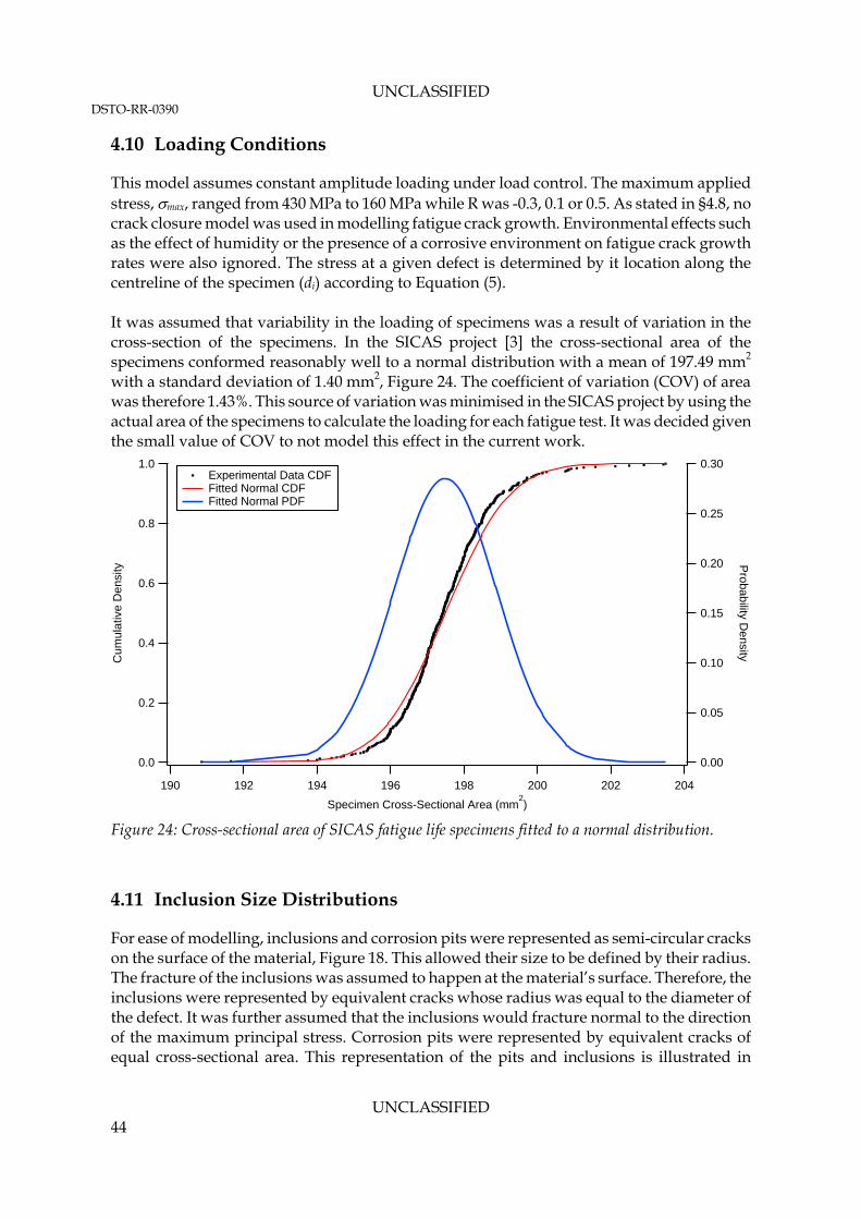
UNCLASSIFIED DSTO-RR-0390
UNCLASSIFIED 44
4.10 Loading Conditions
This model assumes constant amplitude loading under load control. The maximum applied stress, max, ranged from 430 MPa to 160 MPa while R was -0.3, 0.1 or 0.5. As stated in §4.8, no crack closure model was used in modelling fatigue crack growth. Environmental effects such as the effect of humidity or the presence of a corrosive environment on fatigue crack growth rates were also ignored. The stress at a given defect is determined by it location along the centreline of the specimen (di) according to Equation (5). It was assumed that variability in the loading of specimens was a result of variation in the cross-section of the specimens. In the SICAS project [3] the cross-sectional area of the specimens conformed reasonably well to a normal distribution with a mean of 197.49 mm2 with a standard deviation of 1.40 mm2, Figure 24. The coefficient of variation (COV) of area was therefore 1.43%. This source of variation was minimised in the SICAS project by using the actual area of the specimens to calculate the loading for each fatigue test. It was decided given the small value of COV to not model this effect in the current work.
1.0
0.8
0.6
0.4
0.2
0.0
Cum
ulat
ive
Den
sity
204202200198196194192190
Specimen Cross-Sectional Area (mm2)
0.30
0.25
0.20
0.15
0.10
0.05
0.00
Pro
bability D
ensity
Experimental Data CDF Fitted Normal CDF Fitted Normal PDF
Figure 24: Cross-sectional area of SICAS fatigue life specimens fitted to a normal distribution.
4.11 Inclusion Size Distributions
For ease of modelling, inclusions and corrosion pits were represented as semi-circular cracks on the surface of the material, Figure 18. This allowed their size to be defined by their radius. The fracture of the inclusions was assumed to happen at the material’s surface. Therefore, the inclusions were represented by equivalent cracks whose radius was equal to the diameter of the defect. It was further assumed that the inclusions would fracture normal to the direction of the maximum principal stress. Corrosion pits were represented by equivalent cracks of equal cross-sectional area. This representation of the pits and inclusions is illustrated in

UNCLASSIFIED DSTO-RR-0390
UNCLASSIFIED 45
Figure 25. The equivalent radii of the pits, req,pit, and particles, req,particle, are given by Equations (11) and (12), respectively.
pitpiteq Ar 2
, (12)
particleparticleeq dr , (13)
Inclusion
CorrosionPit
Radius
Inclusion diameter= radius of
equivalent crack
Figure 25: Representation of corrosion pits and inclusions in the Criticality Model. Note that the
fracture plane of the inclusion is in the plane of the figure.
The inclusion size distribution was modelled using a Gumbel distribution [5] as this distribution fitted the available inclusion size data better than other extreme value distributions such as the Frechet or Weibull distributions. The cumulative density function (CDF) of the Gumbel distribution is:
0(expexp xxAxFGumbel (14)
where x = the pit depth or radius,
x0 = location parameter, and
A = scale parameter
The corresponding probability density function (PDF) is:
00 (expexp. xxAxxAAxfGumbel (15)
In addition to x0 and A, there is a base area associated with the distribution. The scaled form of this distribution is:
BaseArea
AreaScaledN xxAxF 0(expexp (16)
where ‘Base Area’ = The area of the region from which the observations used to determine the extreme value distribution were obtained, and

UNCLASSIFIED DSTO-RR-0390
UNCLASSIFIED 46
‘Scaled Area’ = The area to which the extreme value distribution is to be applied.
Figure 26 shows the extreme value size distributions for the inclusions. These distributions are shown in their as-measured and scaled forms. The parameters for the as-measured distribution, including the base area, are given in Table 4. A scaling area of 20 mm2 was used. Note that scaling a Gumbel distribution does not change its range. It only translates it left or right along the defect size axis. This behaviour is peculiar to the Gumbel distribution.
1.0
0.8
0.6
0.4
0.2
0.0
Cum
ula
tive
Fre
que
ncy
100806040200
Inclusion Diameter (m)
As-measured Scaled
Figure 26: Comparison of as-measured and scaled corrosion pit and inclusion size distributions used in
the Criticality Model. Arrows labelled ‘Scaling’ show the effect of area scaling on the distribution from the base area used to derive the distribution for a scaled area of 20 mm2.
Table 4: Gumbel distribution parameters for the inclusions used in the Criticality Model as shown in Figure 26.
Parameter X0
(m) A
(m-1) Base Area
(mm2) Scaled Area
(mm2)
Value 16.3336 0.19228 0.185986 20
A source of uncertainty in sizing the inclusions that is not addressed above is what Wicksell called the ‘corpuscle problem’ [112]. As stated, the particle size distribution described above comes from particle size measurements made on a polished surface. This polished surface cuts the particles that appear on it on random planes and at random angles. As such the size of the particles will not be the true size of the particles unless the particles are regular cylinders normal to the polished surface. Examination of Figure 10 shows that the inclusions are clearly not regular cylinders. As such the particle size distribution developed here is only an approximation of the true particle size distribution of the inclusions. This problem cannot be overcome by sampling more particles as it is a fault in the sampling method (i.e. a systematic
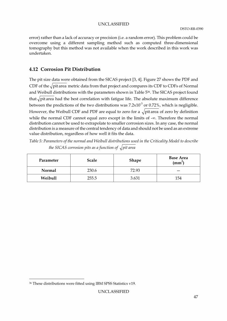
UNCLASSIFIED DSTO-RR-0390
UNCLASSIFIED 47
error) rather than a lack of accuracy or precision (i.e. a random error). This problem could be overcome using a different sampling method such as computed three-dimensional tomography but this method was not available when the work described in this work was undertaken. 4.12 Corrosion Pit Distribution
The pit size data were obtained from the SICAS project [3, 4]. Figure 27 shows the PDF and
CDF of the areapit metric data from that project and compares its CDF to CDFs of Normal
and Weibull distributions with the parameters shown in Table 536. The SICAS project found
that areapit had the best correlation with fatigue life. The absolute maximum difference
between the predictions of the two distributions was 7.2x10⁻³ or 0.72%, which is negligible.
However, the Weibull CDF and PDF are equal to zero for a areapit of zero by definition
while the normal CDF cannot equal zero except in the limits of -∞. Therefore the normal distribution cannot be used to extrapolate to smaller corrosion sizes. In any case, the normal distribution is a measure of the central tendency of data and should not be used as an extreme value distribution, regardless of how well it fits the data.
Table 5: Parameters of the normal and Weibull distributions used in the Criticality Model to describe
the SICAS corrosion pits as a function of areapit
Parameter Scale Shape Base Area (mm2)
Normal 230.6 72.93 —
Weibull 255.5 3.631 154
36 These distributions were fitted using IBM SPSS Statistics v19.

UNCLASSIFIED DSTO-RR-0390
UNCLASSIFIED 48
1.0
0.8
0.6
0.4
0.2
0.0
Nor
mal
ised
Cum
ulat
ive
Fre
quen
cy
5004003002001000
(Pit Area) m
6x10⁻³
5
4
3
2
1
0
Probability D
ensity
SICAS (pit area) Normal CDF Normal PDF WeibullPDF WeibullCDF
Figure 27: The CDF of the areapit metric from the SICAS project compared to Normal and Weibull
distributions fitted to the data. The parameters of these distributions are given in Table 5 above.
Note also that the areapit is not an equivalent radius. To calculate an equivalent radius it is
necessary to divide the areapit by2
. This modifies the Weibull distribution by dividing
the scale parameter by the same value. The scale parameter for a Weibull distribution of equivalent pit radius is therefore 203.9 m. The base area in Table 5 is an estimate of the nominal area of corrosion on each SICAS fatigue specimen. This corrosion was produced by attaching glass tubes to the specimens to be corroded and filling these with an aqueous 3.5 wt% NaCl solution. The tubes were then left in place for ten weeks to allow corrosion to develop. The diameter of the corroded area was around 14 mm which gives an area of 154 mm2. The 14 mm diameter of the corrosion area means that stress at the upper and low points of the area were 0.6% less than at the centre of the area. This is negligible and was ignored in modelling. The use of the SICAS pit size distribution meant, as noted in §4.9, that the fatigue life lookup table for the marker band dataset had to be expanded to defect sizes up to 600 m in radius. 4.13 Crack Metric Ratio
The Crack Metric Ratio (CMR) concept was used in the model to represent the scatter between actual and predicted fatigue lives. The CMR concept was developed in the SICAS project [3, 4] and subsequently used by Shekhter et al. [52] in evaluating the effect of corrosion on the P-3C SLAP method. The CMR is defined as:
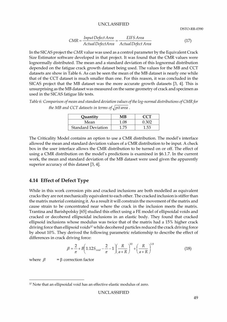
UNCLASSIFIED DSTO-RR-0390
UNCLASSIFIED 49
AreaDefectActual
AreaEIFSAreaDefectActualAreaDefectInput
CMR (17)
In the SICAS project the CMR value was used as a control parameter by the Equivalent Crack Size Estimator software developed in that project. It was found that the CMR values were lognormally distributed. The mean and a standard deviation of this lognormal distribution depended on the fatigue crack growth dataset being used. The values for the MB and CCT datasets are show in Table 6. As can be seen the mean of the MB dataset is nearly one while that of the CCT dataset is much smaller than one. For this reason, it was concluded in the SICAS project that the MB dataset was the more accurate growth datasets [3, 4]. This is unsurprising as the MB dataset was measured on the same geometry of crack and specimen as used in the SICAS fatigue life tests.
Table 6: Comparison of mean and standard deviation values of the log-normal distributions of CMR for the MB and CCT datasets in terms of areapit .
Quantity MB CCT Mean 1.08 0.302
Standard Deviation 1.75 1.53 The Criticality Model contains an option to use a CMR distribution. The model’s interface allowed the mean and standard deviation values of a CMR distribution to be input. A check box in the user interface allows the CMR distribution to be turned on or off. The effect of using a CMR distribution on the model’s predictions is examined in §6.1.7. In the current work, the mean and standard deviation of the MB dataset were used given the apparently superior accuracy of this dataset [3, 4]. 4.14 Effect of Defect Type
While in this work corrosion pits and cracked inclusions are both modelled as equivalent cracks they are not mechanically equivalent to each other. The cracked inclusion is stiffer than the matrix material containing it. As a result it will constrain the movement of the matrix and cause strain to be concentrated near where the crack in the inclusion meets the matrix. Trantina and Barishpolsky [65] studied this effect using a FE model of ellipsoidal voids and cracked or decohered ellipsoidal inclusions in an elastic body. They found that cracked ellipsoid inclusions whose modulus was twice that of the matrix had a 15% higher crack driving force than ellipsoid voids37 while decohered particles reduced the crack driving force by about 10%. They derived the following parametric relationship to describe the effect of differences in crack driving force:
8.110
12
12.12
RaR
RaR
SB void (18)
where = correction factor
37 Note that an ellipsoidal void has an effective elastic modulus of zero.
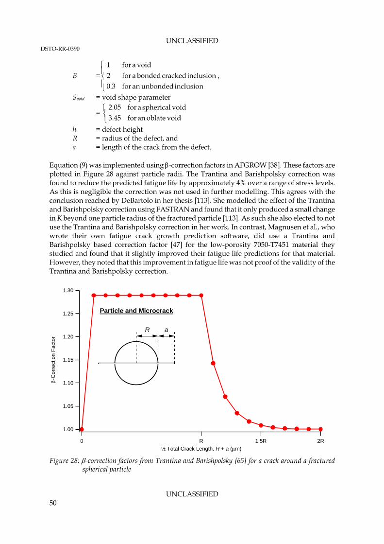
UNCLASSIFIED DSTO-RR-0390
UNCLASSIFIED 50
B =
inclusionunbondedanfor3.0inclusioncrackedbondedafor2
voidafor1,
Svoid = void shape parameter
=
voidoblateanfor45.3voidsphericalafor05.2
h = defect height R = radius of the defect, and a = length of the crack from the defect. Equation (9) was implemented using -correction factors in AFGROW [38]. These factors are plotted in Figure 28 against particle radii. The Trantina and Barishpolsky correction was found to reduce the predicted fatigue life by approximately 4% over a range of stress levels. As this is negligible the correction was not used in further modelling. This agrees with the conclusion reached by DeBartolo in her thesis [113]. She modelled the effect of the Trantina and Barishpolsky correction using FASTRAN and found that it only produced a small change in K beyond one particle radius of the fractured particle [113]. As such she also elected to not use the Trantina and Barishpolsky correction in her work. In contrast, Magnusen et al., who wrote their own fatigue crack growth prediction software, did use a Trantina and Barishpolsky based correction factor [47] for the low-porosity 7050-T7451 material they studied and found that it slightly improved their fatigue life predictions for that material. However, they noted that this improvement in fatigue life was not proof of the validity of the Trantina and Barishpolsky correction.
1.30
1.25
1.20
1.15
1.10
1.05
1.00
-C
orre
ctio
n F
acto
r
0 R 1.5R 2R
½ Total Crack Length, R + a (m)
R
Particle and Microcrack
a
Figure 28: -correction factors from Trantina and Barishpolsky [65] for a crack around a fractured spherical particle
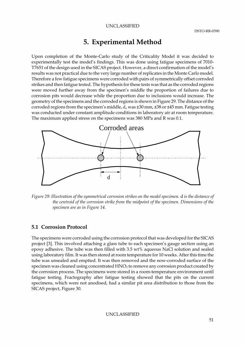
UNCLASSIFIED DSTO-RR-0390
UNCLASSIFIED 51
5. Experimental Method
Upon completion of the Monte-Carlo study of the Criticality Model it was decided to experimentally test the model’s findings. This was done using fatigue specimens of 7010-T7651 of the design used in the SICAS project. However, a direct confirmation of the model’s results was not practical due to the very large number of replicates in the Monte Carlo model. Therefore a few fatigue specimens were corroded with pairs of symmetrically offset corroded strikes and then fatigue tested. The hypothesis for these tests was that as the corroded regions were moved further away from the specimen’s middle the proportion of failures due to corrosion pits would decrease while the proportion due to inclusions would increase. The geometry of the specimens and the corroded regions is shown in Figure 29. The distance of the corroded regions from the specimen’s middle, di, was ±30 mm, ±38 or ±45 mm. Fatigue testing was conducted under constant amplitude conditions in laboratory air at room temperature. The maximum applied stress on the specimens was 380 MPa and R was 0.1.
Corroded areas
d
Figure 29: Illustration of the symmetrical corrosion strikes on the model specimen. d is the distance of
the centroid of the corrosion strike from the midpoint of the specimen. Dimensions of the specimen are as in Figure 14.
5.1 Corrosion Protocol
The specimens were corroded using the corrosion protocol that was developed for the SICAS project [3]. This involved attaching a glass tube to each specimen’s gauge section using an epoxy adhesive. The tube was then filled with 3.5 wt% aqueous NaCl solution and sealed using laboratory film. It was then stored at room temperature for 10 weeks. After this time the tube was unsealed and emptied. It was then removed and the now-corroded surface of the specimen was cleaned using concentrated HNO3 to remove any corrosion product created by the corrosion process. The specimens were stored in a room-temperature environment until fatigue testing. Fractography after fatigue testing showed that the pits on the current specimens, which were not anodised, had a similar pit area distribution to those from the SICAS project, Figure 30.
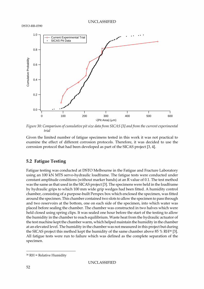
UNCLASSIFIED DSTO-RR-0390
UNCLASSIFIED 52
1.0
0.8
0.6
0.4
0.2
0.0
Cum
ulat
ive P
roba
bilit
y
6005004003002001000
(Pit Area) (m)
Current Experimental Trial SICAS Pit Data
Figure 30: Comparison of cumulative pit size data from SICAS [3] and from the current experimental
trial
Given the limited number of fatigue specimens tested in this work it was not practical to examine the effect of different corrosion protocols. Therefore, it was decided to use the corrosion protocol that had been developed as part of the SICAS project [3, 4]. 5.2 Fatigue Testing
Fatigue testing was conducted at DSTO Melbourne in the Fatigue and Fracture Laboratory using an 100 kN MTS servo-hydraulic loadframe. The fatigue tests were conducted under constant amplitude conditions (without marker bands) at an R value of 0.1. The test method was the same as that used in the SICAS project [3]. The specimens were held in the loadframe by hydraulic grips to which 100 mm wide grip wedges had been fitted. A humidity control chamber, consisting of a purpose-built Perspex box which enclosed the specimen, was fitted around the specimen. This chamber contained two slots to allow the specimen to pass through and two reservoirs at the bottom, one on each side of the specimen, into which water was placed before sealing the chamber. The chamber was constructed in two halves which were held closed using spring clips. It was sealed one hour before the start of the testing to allow the humidity in the chamber to reach equilibrium. Waste heat from the hydraulic actuator of the test machine kept the chamber warm, which helped maintain the humidity in the chamber at an elevated level. The humidity in the chamber was not measured in this project but during the SICAS project this method kept the humidity of the same chamber above 85 % RH38 [3]. All fatigue tests were run to failure which was defined as the complete separation of the specimen. 38 RH = Relative Humidity
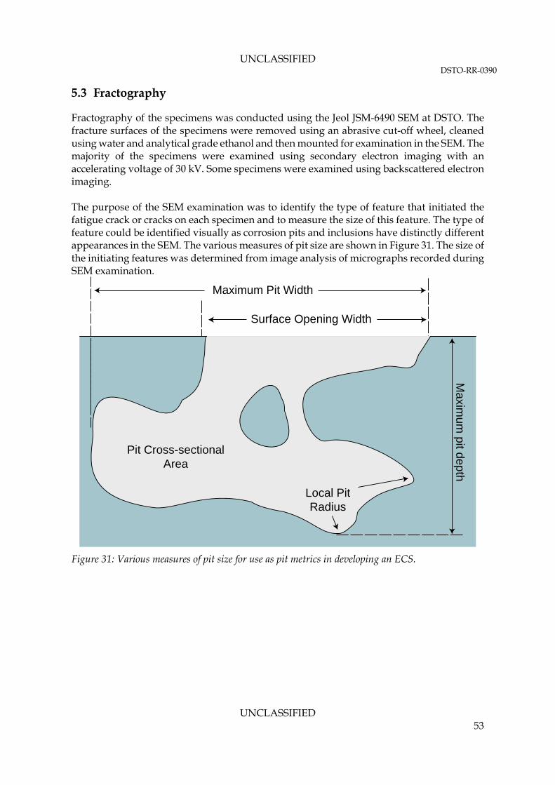
UNCLASSIFIED DSTO-RR-0390
UNCLASSIFIED 53
5.3 Fractography
Fractography of the specimens was conducted using the Jeol JSM-6490 SEM at DSTO. The fracture surfaces of the specimens were removed using an abrasive cut-off wheel, cleaned using water and analytical grade ethanol and then mounted for examination in the SEM. The majority of the specimens were examined using secondary electron imaging with an accelerating voltage of 30 kV. Some specimens were examined using backscattered electron imaging. The purpose of the SEM examination was to identify the type of feature that initiated the fatigue crack or cracks on each specimen and to measure the size of this feature. The type of feature could be identified visually as corrosion pits and inclusions have distinctly different appearances in the SEM. The various measures of pit size are shown in Figure 31. The size of the initiating features was determined from image analysis of micrographs recorded during SEM examination.
Maxim
umpitdepth
Pit Cross-sectionalArea
Surface Opening Width
Maximum Pit Width
Local PitRadius
Figure 31: Various measures of pit size for use as pit metrics in developing an ECS.
UNCLASSIFIED DSTO-RR-0390
UNCLASSIFIED 54
6. Modelling Results
This section reviews the fatigue life and fatigue initiation site predictions of the Criticality Model. It is divided into three sections, which are:
1. Validation and verification of the Criticality Model,
2. Parametric studies, and
3. Prediction of proportion of fatigue failures. 6.1 Validation and Verification of the Criticality Model
The goal of this section is to determine if the Criticality Model’s fatigue life predictions are sensible and correspond with the experimental results from the SICAS project. This validation and verification will be conducted using seven criteria. These criteria are as follows:
1. Comparison of the predicted fatigue lives with SICAS fatigue life results (§6.1.1): The fatigue lives predicted by the model for corroded specimens and uncorroded specimens are compared with the fatigue life data from the SICAS project. This comparison is made as a function of applied stress at load ratios of -0.3, 0.1 and 0.5 for the corroded material and R = 0.1 for the uncorroded material. These load ratios correspond to those used in the SICAS project.
2. Effect of the number of replicates (§6.1.2): The convergence of the Criticality Model is tested in this section by examining the trend in the sum of the scatter in the model’s predictions versus the number of replicates. This trend is compared to the inverse square root convergence expected of a Monte Carlo model.
3. Execution Times (§6.1.3): This section examines the time required for the model to complete a set of predictions as a function of the number of replicates and the number of defects being modelled. This combined with the study of the number of replicates was used to select the optimal number of replicates to be used in subsequent modelling.
4. Comparison of Probabilistic and Deterministic Life Predictions (§6.1.4): In this section the model’s probabilistic fatigue life predictions are compared with deterministic fatigue lives calculated using AFGROW. Ideally the model should not alter the predicted fatigue lives for a given defect size and applied stress.
5. Effect of Area per Defect (§6.1.5): The area per defect affects the execution speed of the model as it controls the numbers of pit and inclusions simulated in each iteration of the model. In this section the effect of using area per defect values ranging between 0.19 and 154 mm2 for the pits and inclusions was examined. This criteria is satisfied if the area per defect does not alter the predictions of fatigue life and failure location the for the above range of values.
6. Effect of Stress Level (§6.1.6): This section examines how the applied stress level affects the shape of the normalised fatigue life vs. exceedance and failure location vs. exceedance curves. The normalised fatigue life vs. exceedance curve is created by

UNCLASSIFIED DSTO-RR-0390
UNCLASSIFIED 55
dividing the fatigue lives of the curves by the median lives of each curve at the four stress levels examined.
7. Effect of SICAS Crack Metric Ratio Correction (§6.1.7): Finally, the effect on the model’s fatigue life predictions of using the mean crack metro ratio of 1.08 from the SICAS project was examined. The effect of the using the CMR is compared with the results obtained in the SICAS project.
Of the above Criteria 1, 3 5 and 7 are validation criteria as they do compare the model’s prediction with experimental data , while Criteria 2, 4 and 6 are verification criteria as they only compare the model against theoretical outputs39. If the model complies with each of the above criteria its predictions are expected to be of good quality. 6.1.1 Comparison of Predicted and SICAS Experimental Fatigue Lives
The first step in validating and verifying the Criticality Model was to compares its fatigue life predictions to the experimental lives recorded in the SICAS project [3, 4]. This comparison is made for the corroded specimens in Figure 32, Figure 33, Figure 34 for R values of 0.1, 0.5 and -0.3 respectively. The correspondence between the predicted fatigue lives and the actual fatigue lives is excellent at all three load ratios. Specifically, the model was able to accurately predict the lower bound and median fatigue lives at all three R values. However, it did not predict the scatter in fatigue lives at low maximum stress values. This is probably because the model cannot predict the cycles consumed by crack nucleation processes, which are the likely cause of the observed scatter.
39 The definitions of ‘Verification’ and ‘Validation’ used here come from the ASME Guide for Verification and Validation in Computational Solid Mechanics [114] and are as follows:
Verification: The process of determining that a computational model accurately represents the underlying mathematical model and its solution.
Validation: The process of determining the degree to which a model is an accurate representation of the real world from the perspective of the intended use of the model.

UNCLASSIFIED DSTO-RR-0390
UNCLASSIFIED 56
400
350
300
250
200
150
Max
imum
Str
ess
(MP
a)
104
105
106
107
Cycles to failure (Nf)
SICAS Corroded R = 0.1 Model p = 0.001 Model p = 0.500 Model p = 0.995
Figure 32: Comparison of SICAS fatigue life results for specimens that were both anodised and
corroded at R = 0.1 with the predictions of the Criticality Model. The number of replicates was 5,000. The area per pit and inclusion was 153.94 mm2.
450
400
350
300
250
200
150
Ma
xim
um S
tre
ss (
MP
a)
104
2 3 4 5 6 7 8 9
105
2 3 4 5 6 7 8 9
106
2 3 4 5 6 7 8 9
107
Cycles to Failure
SICAS Corroded R = 0.5 Model p = 0.001 Model p = 0.500 Model p = 0.999
Figure 33: Comparison of SICAS fatigue life results for specimens that were both anodised and
corroded at R = 0.5 with the predictions of the Criticality Model. The specimens were made from AA7010-T7651.
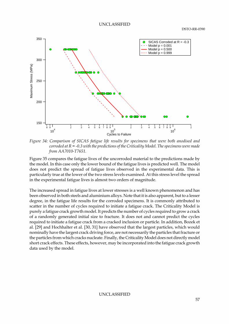
UNCLASSIFIED DSTO-RR-0390
UNCLASSIFIED 57
350
300
250
200
150
Max
imum
Str
ess
(MP
a)
8 9
104
2 3 4 5 6 7 8 9
105
2 3 4 5 6 7 8 9
106
2
Cycles to Failure
SICAS Corroded at R = -0.3 Model p = 0.001 Model p = 0.500 Model p = 0.999
Figure 34: Comparison of SICAS fatigue life results for specimens that were both anodised and
corroded at R = -0.3 with the predictions of the Criticality Model. The specimens were made from AA7010-T7651.
Figure 35 compares the fatigue lives of the uncorroded material to the predictions made by the model. In this case only the lower bound of the fatigue lives is predicted well. The model does not predict the spread of fatigue lives observed in the experimental data. This is particularly true at the lower of the two stress levels examined. At this stress level the spread in the experimental fatigue lives is almost two orders of magnitude. The increased spread in fatigue lives at lower stresses is a well known phenomenon and has been observed in both steels and aluminium alloys. Note that it is also apparent, but to a lesser degree, in the fatigue life results for the corroded specimens. It is commonly attributed to scatter in the number of cycles required to initiate a fatigue crack. The Criticality Model is purely a fatigue crack growth model. It predicts the number of cycles required to grow a crack of a randomly generated initial size to fracture. It does not and cannot predict the cycles required to initiate a fatigue crack from a cracked inclusion or particle. In addition, Bozek et al. [29] and Hochhalter et al. [30, 31] have observed that the largest particles, which would nominally have the largest crack driving force, are not necessarily the particles that fracture or the particles from which cracks nucleate. Finally, the Criticality Model does not directly model short crack effects. These effects, however, may be incorporated into the fatigue crack growth data used by the model.

UNCLASSIFIED DSTO-RR-0390
UNCLASSIFIED 58
400
350
300
250
200
150
Max
imum
Str
ess
(MP
a)
104
105
106
107
Cycles to failure (Nf)
SICAS Anodised R = 0.1 SICAS As-Machined R = 0.1 Model p = 0.005 Model p = 0.500 Model p = 0.995
Figure 35: Comparison of the model’s prediction using the MB dataset with the SICAS fatigue life
results at R = 0.1 for uncorroded specimens that were either anodised or in the as-machined state. The specimens were made from AA7010-T7651. The area per pit and inclusion was 153.94 mm2.
6.1.2 Effect of the Number of Replicates
The accuracy of Monte Carlo models increases as more replicates are made. Specifically, the error in the predictions of a Monte Carlo simulation decreases as the number of iterations increases according to the relationship [115]:
n
Error1
(19)
Where n = the number of iterations. Given the above, the accuracy of a Monte Carlo simulation can be increased by increasing the number of iterations, n. However, this increases calculation time and so a balance needs to be struck between accuracy and calculation time. To this end a series of simulations using the Criticality Model were run with different n values to measure the scatter in the predictions of the Criticality Model. The model was run eight times at each n value. The minimum and maximum fatigue life predictions as a function of exceedance were calculated from this set of eight runs. These are shown in Figure 36 versus exceedance. The range in fatigue life predictions at each n value was then calculated. These are plotted against exceedance in Figure 37. These figures show that the scatter decreases as n increases. The maximum fatigue life ranges between exceedance values of 0.4 and 0.95 were measured for each n value and plotted versus n in Figure 38. A power law was fitted to fitted to these data and was found to have an exponent of approximately -0.5, which is equivalent to Equation (19) above. Therefore, the Criticality Model is showing the convergence behaviour expected for a Monte Carlo simulation. From Figure 38 it was decided that n = 5,000 gave a good balance between accuracy and computational speed. All further modelling used this value of n.
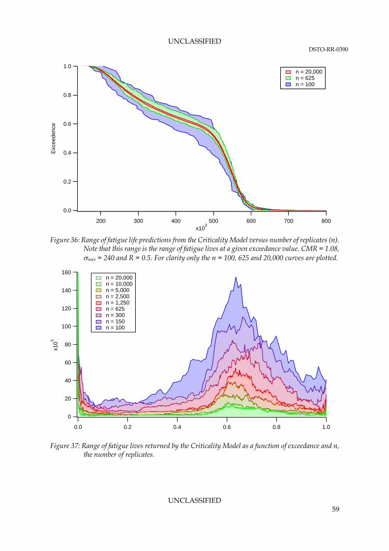
UNCLASSIFIED DSTO-RR-0390
UNCLASSIFIED 59
1.0
0.8
0.6
0.4
0.2
0.0
Exc
eed
ence
800700600500400300200x10
3
n = 20,000 n = 625 n = 100
Figure 36: Range of fatigue life predictions from the Criticality Model versus number of replicates (n).
Note that this range is the range of fatigue lives at a given exceedance value. CMR = 1.08, max = 240 and R = 0.5. For clarity only the n = 100, 625 and 20,000 curves are plotted.
160
140
120
100
80
60
40
20
0
x103
1.00.80.60.40.20.0
n = 20,000 n = 10,000 n = 5,000 n = 2,500 n = 1,250 n = 625 n = 300 n = 150 n = 100
Figure 37: Range of fatigue lives returned by the Criticality Model as a function of exceedance and n,
the number of replicates.

UNCLASSIFIED DSTO-RR-0390
UNCLASSIFIED 60
5.0
4.5
4.0
3.5
3.0
Log 1
0(M
ean
Err
or R
ange
)
4.54.03.53.02.52.0Log10(Iterations)
Function: lineCoefficient values ± 99% Confidence Interval
a =5.767 ± 0.163b =-0.50829 ± 0.051
Mean Error Range Linear Curve Fit 99% Confidence Interval
Figure 38: Fit of log10(mean fatigue life range) vs. log10(iterations) to a linear least squares fit for the
Criticality Model.
6.1.3 Execution Times
This section examines the effect of the number of replicates, inclusions and corrosion pits being modelled on the execution time of the Criticality Model. The minimum number of pits modelled was one per iteration while the maximum was 840. The maximum number of pits came from assuming a base area per pit each to 0.185 mm2, which is the base area for the extreme value size distribution of the inclusions. The number of iterations varied between 100 and 20,000. Figure 39 plots the execution time of the model as a function of the number of pits being modelled per iteration of the model and the number of iterations of the model. The execution time varied from 1.55 seconds for 1 pit and 100 iterations to 2,300 seconds (38.5 minutes) for 840 pits and 20,000 iterations. The execution time was more strongly affected by the number of iterations than by the number of pits per iteration. This indicates that the generation of the model specimen per iteration was optimised while the iteration between specimens was not.
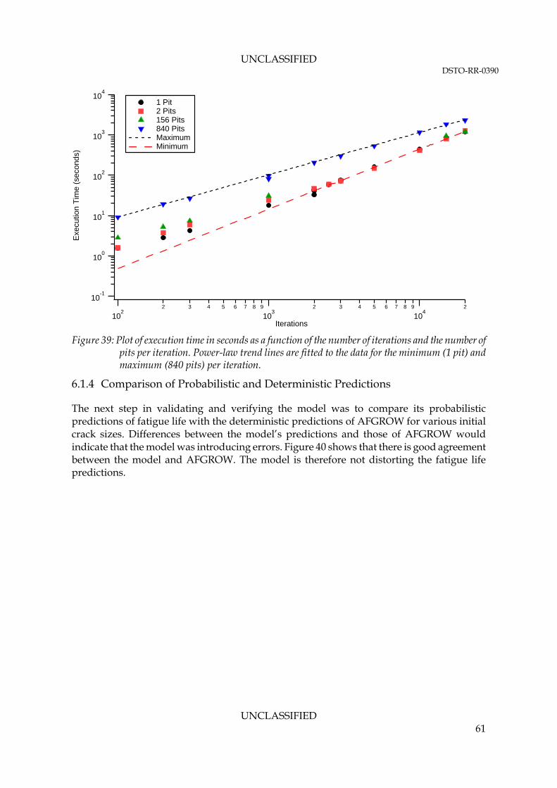
UNCLASSIFIED DSTO-RR-0390
UNCLASSIFIED 61
10-1
100
101
102
103
104
Exe
cutio
n T
ime
(sec
onds
)
102
2 3 4 5 6 7 8 9
103
2 3 4 5 6 7 8 9
104
2
Iterations
1 Pit 2 Pits 156 Pits 840 Pits Maximum Minimum
Figure 39: Plot of execution time in seconds as a function of the number of iterations and the number of
pits per iteration. Power-law trend lines are fitted to the data for the minimum (1 pit) and maximum (840 pits) per iteration.
6.1.4 Comparison of Probabilistic and Deterministic Predictions
The next step in validating and verifying the model was to compare its probabilistic predictions of fatigue life with the deterministic predictions of AFGROW for various initial crack sizes. Differences between the model’s predictions and those of AFGROW would indicate that the model was introducing errors. Figure 40 shows that there is good agreement between the model and AFGROW. The model is therefore not distorting the fatigue life predictions.
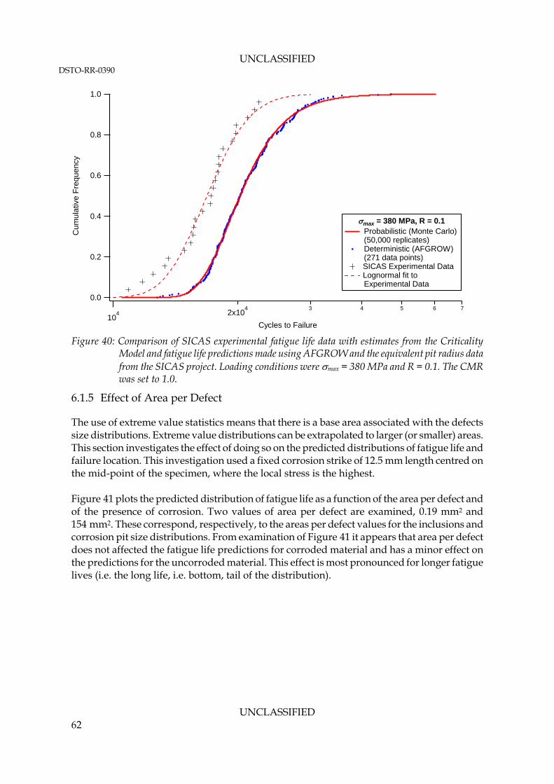
UNCLASSIFIED DSTO-RR-0390
UNCLASSIFIED 62
1.0
0.8
0.6
0.4
0.2
0.0
Cu
mu
lativ
e F
req
ue
ncy
104 2x10
4 3 4 5 6 7
Cycles to Failure
max = 380 MPa, R = 0.1Probabilistic (Monte Carlo) (50,000 replicates)
Deterministic (AFGROW)(271 data points)
SICAS Experimental Data Lognormal fit toExperimental Data
Figure 40: Comparison of SICAS experimental fatigue life data with estimates from the Criticality
Model and fatigue life predictions made using AFGROW and the equivalent pit radius data from the SICAS project. Loading conditions were max = 380 MPa and R = 0.1. The CMR was set to 1.0.
6.1.5 Effect of Area per Defect
The use of extreme value statistics means that there is a base area associated with the defects size distributions. Extreme value distributions can be extrapolated to larger (or smaller) areas. This section investigates the effect of doing so on the predicted distributions of fatigue life and failure location. This investigation used a fixed corrosion strike of 12.5 mm length centred on the mid-point of the specimen, where the local stress is the highest. Figure 41 plots the predicted distribution of fatigue life as a function of the area per defect and of the presence of corrosion. Two values of area per defect are examined, 0.19 mm2 and 154 mm2. These correspond, respectively, to the areas per defect values for the inclusions and corrosion pit size distributions. From examination of Figure 41 it appears that area per defect does not affected the fatigue life predictions for corroded material and has a minor effect on the predictions for the uncorroded material. This effect is most pronounced for longer fatigue lives (i.e. the long life, i.e. bottom, tail of the distribution).
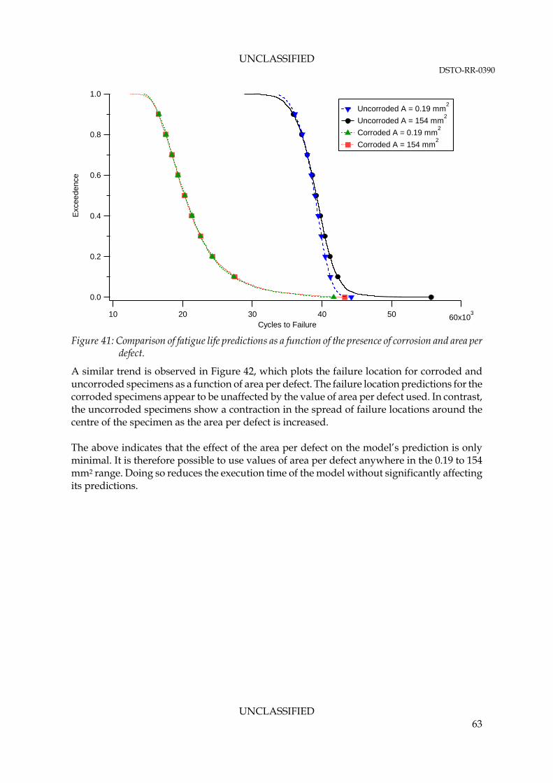
UNCLASSIFIED DSTO-RR-0390
UNCLASSIFIED 63
1.0
0.8
0.6
0.4
0.2
0.0
Exc
eedenc
e
60x1035040302010
Cycles to Failure
Uncorroded A = 0.19 mm2
Uncorroded A = 154 mm2
Corroded A = 0.19 mm2
Corroded A = 154 mm2
Figure 41: Comparison of fatigue life predictions as a function of the presence of corrosion and area per
defect.
A similar trend is observed in Figure 42, which plots the failure location for corroded and uncorroded specimens as a function of area per defect. The failure location predictions for the corroded specimens appear to be unaffected by the value of area per defect used. In contrast, the uncorroded specimens show a contraction in the spread of failure locations around the centre of the specimen as the area per defect is increased. The above indicates that the effect of the area per defect on the model’s prediction is only minimal. It is therefore possible to use values of area per defect anywhere in the 0.19 to 154 mm2 range. Doing so reduces the execution time of the model without significantly affecting its predictions.
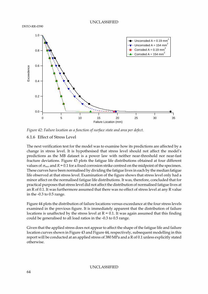
UNCLASSIFIED DSTO-RR-0390
UNCLASSIFIED 64
1.0
0.8
0.6
0.4
0.2
0.0
Exc
eedenc
e
35302520151050Failure Location (mm)
Uncorroded A = 0.19 mm2
Uncorroded A = 154 mm2
Corroded A = 0.19 mm2
Corroded A = 154 mm2
Figure 42: Failure location as a function of surface state and area per defect.
6.1.6 Effect of Stress Level
The next verification test for the model was to examine how its predictions are affected by a change in stress level. It is hypothesised that stress level should not affect the model’s predictions as the MB dataset is a power law with neither near-threshold nor near-fast fracture deviations. Figure 43 plots the fatigue life distributions obtained at four different values of max and R = 0.1 for a fixed corrosion strike centred on the midpoint of the specimen. These curves have been normalised by dividing the fatigue lives in each by the median fatigue life observed at that stress level. Examination of the figure shows that stress level only had a minor affect on the normalised fatigue life distributions. It was, therefore, concluded that for practical purposes that stress level did not affect the distribution of normalised fatigue lives at an R of 0.1. It was furthermore assumed that there was no effect of stress level at any R value in the -0.3 to 0.5 range. Figure 44 plots the distribution of failure locations versus exceedance at the four stress levels examined in the previous figure. It is immediately apparent that the distribution of failure locations is unaffected by the stress level at R = 0.1. It was again assumed that this finding could be generalised to all load ratios in the -0.3 to 0.5 range. Given that the applied stress does not appear to affect the shape of the fatigue life and failure location curves shown in Figure 43 and Figure 44, respectively, subsequent modelling in this report will be conducted at an applied stress of 380 MPa and a R of 0.1 unless explicitly stated otherwise.
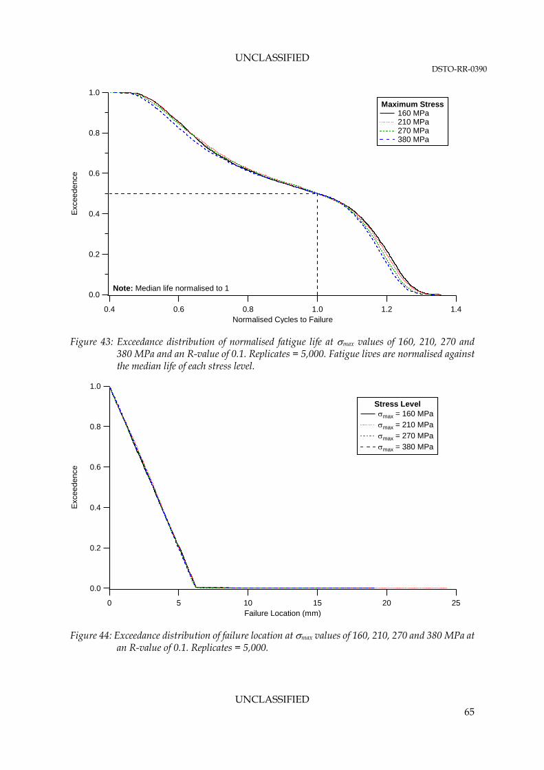
UNCLASSIFIED DSTO-RR-0390
UNCLASSIFIED 65
1.0
0.8
0.6
0.4
0.2
0.0
Exc
eed
ence
1.41.21.00.80.60.4Normalised Cycles to Failure
Maximum Stress 160 MPa 210 MPa 270 MPa 380 MPa
Note: Median life normalised to 1
Figure 43: Exceedance distribution of normalised fatigue life at max values of 160, 210, 270 and 380 MPa and an R-value of 0.1. Replicates = 5,000. Fatigue lives are normalised against the median life of each stress level.
1.0
0.8
0.6
0.4
0.2
0.0
Exc
eed
ence
2520151050Failure Location (mm)
Stress Level max = 160 MPa
max = 210 MPa
max = 270 MPa
max = 380 MPa
Figure 44: Exceedance distribution of failure location at max values of 160, 210, 270 and 380 MPa at an R-value of 0.1. Replicates = 5,000.
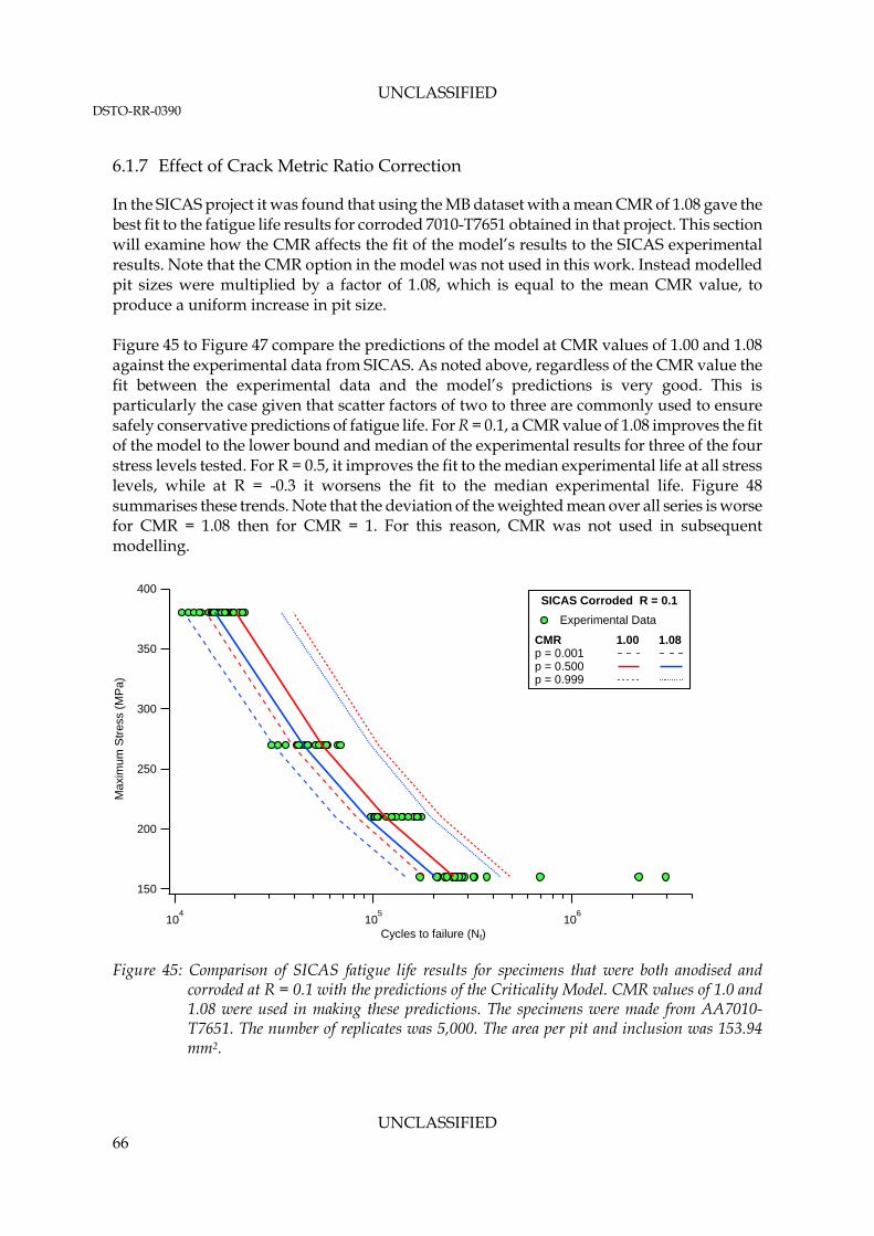
UNCLASSIFIED DSTO-RR-0390
UNCLASSIFIED 66
6.1.7 Effect of Crack Metric Ratio Correction
In the SICAS project it was found that using the MB dataset with a mean CMR of 1.08 gave the best fit to the fatigue life results for corroded 7010-T7651 obtained in that project. This section will examine how the CMR affects the fit of the model’s results to the SICAS experimental results. Note that the CMR option in the model was not used in this work. Instead modelled pit sizes were multiplied by a factor of 1.08, which is equal to the mean CMR value, to produce a uniform increase in pit size. Figure 45 to Figure 47 compare the predictions of the model at CMR values of 1.00 and 1.08 against the experimental data from SICAS. As noted above, regardless of the CMR value the fit between the experimental data and the model’s predictions is very good. This is particularly the case given that scatter factors of two to three are commonly used to ensure safely conservative predictions of fatigue life. For R = 0.1, a CMR value of 1.08 improves the fit of the model to the lower bound and median of the experimental results for three of the four stress levels tested. For R = 0.5, it improves the fit to the median experimental life at all stress levels, while at R = -0.3 it worsens the fit to the median experimental life. Figure 48 summarises these trends. Note that the deviation of the weighted mean over all series is worse for CMR = 1.08 then for CMR = 1. For this reason, CMR was not used in subsequent modelling.
400
350
300
250
200
150
Max
imum
Str
ess
(MP
a)
104
105
106
Cycles to failure (Nf)
SICAS Corroded R = 0.1
Experimental Data
CMR 1.00 1.08 p = 0.001 p = 0.500 p = 0.999
Figure 45: Comparison of SICAS fatigue life results for specimens that were both anodised and corroded at R = 0.1 with the predictions of the Criticality Model. CMR values of 1.0 and 1.08 were used in making these predictions. The specimens were made from AA7010-T7651. The number of replicates was 5,000. The area per pit and inclusion was 153.94 mm2.
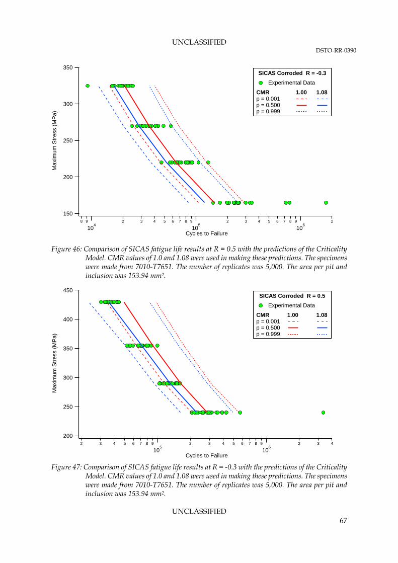
UNCLASSIFIED DSTO-RR-0390
UNCLASSIFIED 67
350
300
250
200
150
Max
imum
Str
ess
(MP
a)
8 9
104
2 3 4 5 6 7 8 9
105
2 3 4 5 6 7 8 9
106
2
Cycles to Failure
SICAS Corroded R = -0.3
Experimental Data
CMR 1.00 1.08 p = 0.001 p = 0.500 p = 0.999
Figure 46: Comparison of SICAS fatigue life results at R = 0.5 with the predictions of the Criticality Model. CMR values of 1.0 and 1.08 were used in making these predictions. The specimens were made from 7010-T7651. The number of replicates was 5,000. The area per pit and inclusion was 153.94 mm2.
450
400
350
300
250
200
Max
imum
Str
ess
(MP
a)
2 3 4 5 6 7 8 9
105
2 3 4 5 6 7 8 9
106
2 3 4
Cycles to Failure
SICAS Corroded R = 0.5
Experimental Data
CMR 1.00 1.08 p = 0.001 p = 0.500 p = 0.999
Figure 47: Comparison of SICAS fatigue life results at R = -0.3 with the predictions of the Criticality
Model. CMR values of 1.0 and 1.08 were used in making these predictions. The specimens were made from 7010-T7651. The number of replicates was 5,000. The area per pit and inclusion was 153.94 mm2.
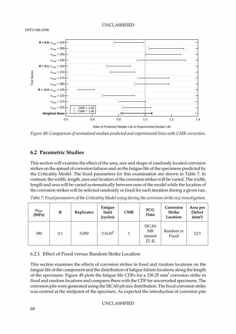
UNCLASSIFIED DSTO-RR-0390
UNCLASSIFIED 68
R = 0.5: max = 240
max = 290
max = 355
max = 430
R = 0.1: max = 160
max = 210
max = 270
max = 380
R = -0.3: max = 165
max = 220
max = 270
max = 325
Weighted Mean
Tes
t Ser
ies
1.41.21.00.80.60.4
Ratio of Predicted Median Life to Experimental Median Life
CMR = 1.00 CMR = 1.08
Figure 48: Comparison of normalised median predicted and experimental lives with CMR correction.
6.2 Parametric Studies
This section will examine the effect of the area, size and shape of randomly located corrosion strikes on the spread of corrosion failures and on the fatigue life of the specimens predicted by the Criticality Model. The fixed parameters for this examination are shown in Table 7. In contrast, the width, length, area and location of the corrosion strikes will be varied. The width, length and area will be varied systematically between runs of the model while the location of the corrosion strikes will be selected randomly or fixed for each iteration during a given run.
Table 7: Fixed parameters of the Criticality Model using during the corrosion strike size investigation.
max (MPa)
R Replicates Fatigue
limit (cycles)
CMR FCG Data
Corrosion Strike
Location
Area per Defect (mm2)
380 0.1 5,000 3.5x10⁶ 1
SICAS MB
dataset [3, 4]
Random or Fixed
12.5
6.2.1 Effect of Fixed versus Random Strike Location
This section examines the effects of corrosion strikes in fixed and random locations on the fatigue life of the component and the distribution of fatigue failure locations along the length of the specimens. Figure 49 plots the fatigue life CDFs for a 156.25 mm2 corrosion strike in fixed and random locations and compares these with the CDF for uncorroded specimens. The corrosion pits were generated using the SICAS pit size distribution. The fixed corrosion strike was centred at the midpoint of the specimen. As expected the introduction of corrosion pits
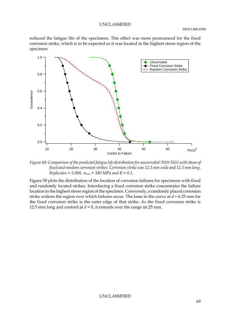
UNCLASSIFIED DSTO-RR-0390
UNCLASSIFIED 69
reduced the fatigue life of the specimens. This effect was more pronounced for the fixed corrosion strike, which is to be expected as it was located in the highest stress region of the specimen.
1.0
0.8
0.6
0.4
0.2
0.0
Exc
ee
den
ce
70x103605040302010
Cycles to Failure
Uncorroded Fixed Corrosion Strike Random Corrosion Strike
Figure 49: Comparison of the predicted fatigue life distribution for uncorroded 7010-T651 with those of fixed and random corrosion strikes. Corrosion strike was 12.5 mm wide and 12.5 mm long. Replicates = 5,000, max = 380 MPa and R = 0.1.
Figure 50 plots the distribution of the location of corrosion failures for specimens with fixed and randomly located strikes. Introducing a fixed corrosion strike concentrates the failure location in the highest stress region of the specimen. Conversely, a randomly placed corrosion strike widens the region over which failures occur. The knee in the curve at d = 6.25 mm for the fixed corrosion strike is the outer edge of that strike. As the fixed corrosion strike is 12.5 mm long and centred at d = 0, it extends over the range ±6.25 mm.
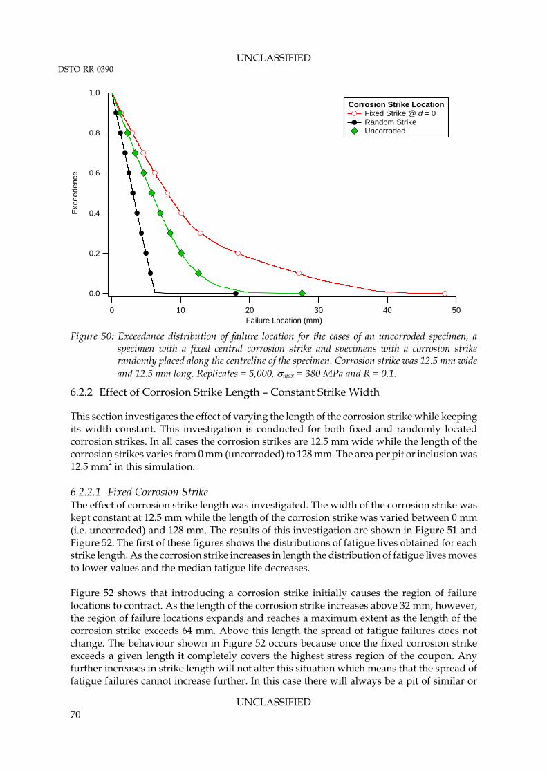
UNCLASSIFIED DSTO-RR-0390
UNCLASSIFIED 70
1.0
0.8
0.6
0.4
0.2
0.0
Exc
eed
enc
e
50403020100Failure Location (mm)
Corrosion Strike Location Fixed Strike @ d = 0 Random Strike Uncorroded
Figure 50: Exceedance distribution of failure location for the cases of an uncorroded specimen, a
specimen with a fixed central corrosion strike and specimens with a corrosion strike randomly placed along the centreline of the specimen. Corrosion strike was 12.5 mm wide and 12.5 mm long. Replicates = 5,000, max = 380 MPa and R = 0.1.
6.2.2 Effect of Corrosion Strike Length – Constant Strike Width
This section investigates the effect of varying the length of the corrosion strike while keeping its width constant. This investigation is conducted for both fixed and randomly located corrosion strikes. In all cases the corrosion strikes are 12.5 mm wide while the length of the corrosion strikes varies from 0 mm (uncorroded) to 128 mm. The area per pit or inclusion was 12.5 mm2 in this simulation. 6.2.2.1 Fixed Corrosion Strike The effect of corrosion strike length was investigated. The width of the corrosion strike was kept constant at 12.5 mm while the length of the corrosion strike was varied between 0 mm (i.e. uncorroded) and 128 mm. The results of this investigation are shown in Figure 51 and Figure 52. The first of these figures shows the distributions of fatigue lives obtained for each strike length. As the corrosion strike increases in length the distribution of fatigue lives moves to lower values and the median fatigue life decreases. Figure 52 shows that introducing a corrosion strike initially causes the region of failure locations to contract. As the length of the corrosion strike increases above 32 mm, however, the region of failure locations expands and reaches a maximum extent as the length of the corrosion strike exceeds 64 mm. Above this length the spread of fatigue failures does not change. The behaviour shown in Figure 52 occurs because once the fixed corrosion strike exceeds a given length it completely covers the highest stress region of the coupon. Any further increases in strike length will not alter this situation which means that the spread of fatigue failures cannot increase further. In this case there will always be a pit of similar or
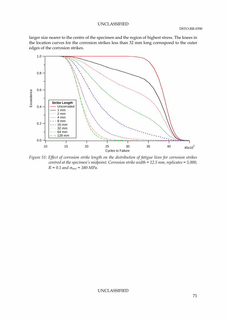
UNCLASSIFIED DSTO-RR-0390
UNCLASSIFIED 71
larger size nearer to the centre of the specimen and the region of highest stress. The knees in the location curves for the corrosion strikes less than 32 mm long correspond to the outer edges of the corrosion strikes.
1.0
0.8
0.6
0.4
0.2
0.0
Exc
eed
ence
45x10340353025201510
Cycles to Failure
Strike Length Uncorroded 1 mm 2 mm 4 mm 8 mm 16 mm 32 mm 64 mm 128 mm
Figure 51: Effect of corrosion strike length on the distribution of fatigue lives for corrosion strikes
centred at the specimen’s midpoint. Corrosion strike width = 12.5 mm, replicates = 5,000, R = 0.1 and max = 380 MPa.

UNCLASSIFIED DSTO-RR-0390
UNCLASSIFIED 72
1.0
0.8
0.6
0.4
0.2
0.0
Exc
eed
ence
2520151050Failure Location (mm)
Strike Length Uncorroded 1 mm 2 mm 4 mm 8 mm 16 mm 32 mm 64 mm 128 mm
Figure 52: Effect of corrosion strike length on the distribution of fatigue failure locations for corrosion
strikes centred at the specimen’s midpoint. Corrosion strike width = 12.5 mm, replicates = 5000, R = 0.1 and max = 380 MPa.
6.2.2.2 Random Corrosion Strike As with the centrally fixed corrosion strike (Figure 51), a randomly placed corrosion reduces the fatigue life of the component, Figure 53. This reduction however is less pronounced than for the fixed corrosion strike. This is because, unlike the fixed corrosion strike examined above, the random strike is not necessarily located in the highest stress region of the component.

UNCLASSIFIED DSTO-RR-0390
UNCLASSIFIED 73
1.0
0.8
0.6
0.4
0.2
0.0
Exc
eed
ence
50x1034540353025201510
Cycles to Failure
Strike Length Uncorroded 1 mm 2 mm 4 mm 8 mm 16 mm 32 mm 64 mm 128 mm
Figure 53: Effect of corrosion strike length on the distribution of fatigue lives for randomly located
corrosion strikes. Corrosion strike width = 12.5 mm, replicates = 5000, R = 0.1 and max = 380 MPa.
Figure 54 shows that introducing a random corrosion strike greatly expands the range of locations over which failures can occur. This is in contrast to a fixed central strike which contracts this range, Figure 52. There is an indication, however, that once the randomly located corrosion strike exceeds 64 mm in length the region of fatigue failure locations begins to contract. This is probably because the corrosion strike is now almost certain to cross the central region of the component where the stresses are highest.
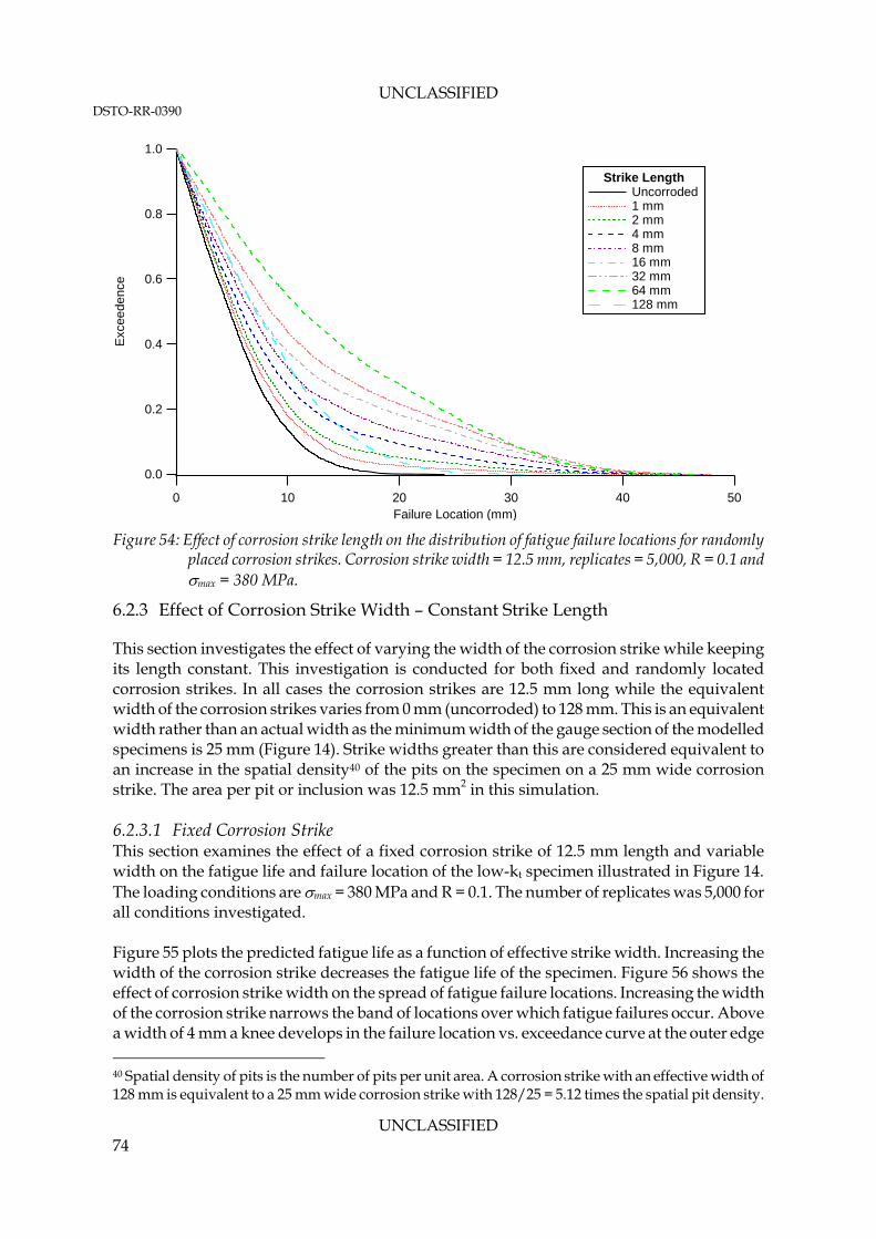
UNCLASSIFIED DSTO-RR-0390
UNCLASSIFIED 74
1.0
0.8
0.6
0.4
0.2
0.0
Exc
eed
ence
50403020100Failure Location (mm)
Strike Length Uncorroded 1 mm 2 mm 4 mm 8 mm 16 mm 32 mm 64 mm 128 mm
Figure 54: Effect of corrosion strike length on the distribution of fatigue failure locations for randomly
placed corrosion strikes. Corrosion strike width = 12.5 mm, replicates = 5,000, R = 0.1 and max = 380 MPa.
6.2.3 Effect of Corrosion Strike Width – Constant Strike Length
This section investigates the effect of varying the width of the corrosion strike while keeping its length constant. This investigation is conducted for both fixed and randomly located corrosion strikes. In all cases the corrosion strikes are 12.5 mm long while the equivalent width of the corrosion strikes varies from 0 mm (uncorroded) to 128 mm. This is an equivalent width rather than an actual width as the minimum width of the gauge section of the modelled specimens is 25 mm (Figure 14). Strike widths greater than this are considered equivalent to an increase in the spatial density40 of the pits on the specimen on a 25 mm wide corrosion strike. The area per pit or inclusion was 12.5 mm2 in this simulation. 6.2.3.1 Fixed Corrosion Strike This section examines the effect of a fixed corrosion strike of 12.5 mm length and variable width on the fatigue life and failure location of the low-kt specimen illustrated in Figure 14. The loading conditions are max = 380 MPa and R = 0.1. The number of replicates was 5,000 for all conditions investigated. Figure 55 plots the predicted fatigue life as a function of effective strike width. Increasing the width of the corrosion strike decreases the fatigue life of the specimen. Figure 56 shows the effect of corrosion strike width on the spread of fatigue failure locations. Increasing the width of the corrosion strike narrows the band of locations over which fatigue failures occur. Above a width of 4 mm a knee develops in the failure location vs. exceedance curve at the outer edge 40 Spatial density of pits is the number of pits per unit area. A corrosion strike with an effective width of 128 mm is equivalent to a 25 mm wide corrosion strike with 128/25 = 5.12 times the spatial pit density.
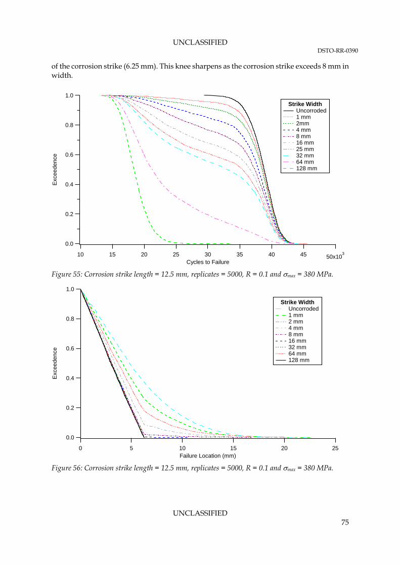
UNCLASSIFIED DSTO-RR-0390
UNCLASSIFIED 75
of the corrosion strike (6.25 mm). This knee sharpens as the corrosion strike exceeds 8 mm in width.
1.0
0.8
0.6
0.4
0.2
0.0
Exc
eed
ence
50x1034540353025201510
Cycles to Failure
Strike Width Uncorroded 1 mm 2mm 4 mm 8 mm 16 mm 25 mm 32 mm 64 mm 128 mm
Figure 55: Corrosion strike length = 12.5 mm, replicates = 5000, R = 0.1 and max = 380 MPa.
1.0
0.8
0.6
0.4
0.2
0.0
Exc
eed
ence
2520151050Failure Location (mm)
Strike Width Uncorroded 1 mm 2 mm 4 mm 8 mm 16 mm 32 mm 64 mm 128 mm
Figure 56: Corrosion strike length = 12.5 mm, replicates = 5000, R = 0.1 and max = 380 MPa.
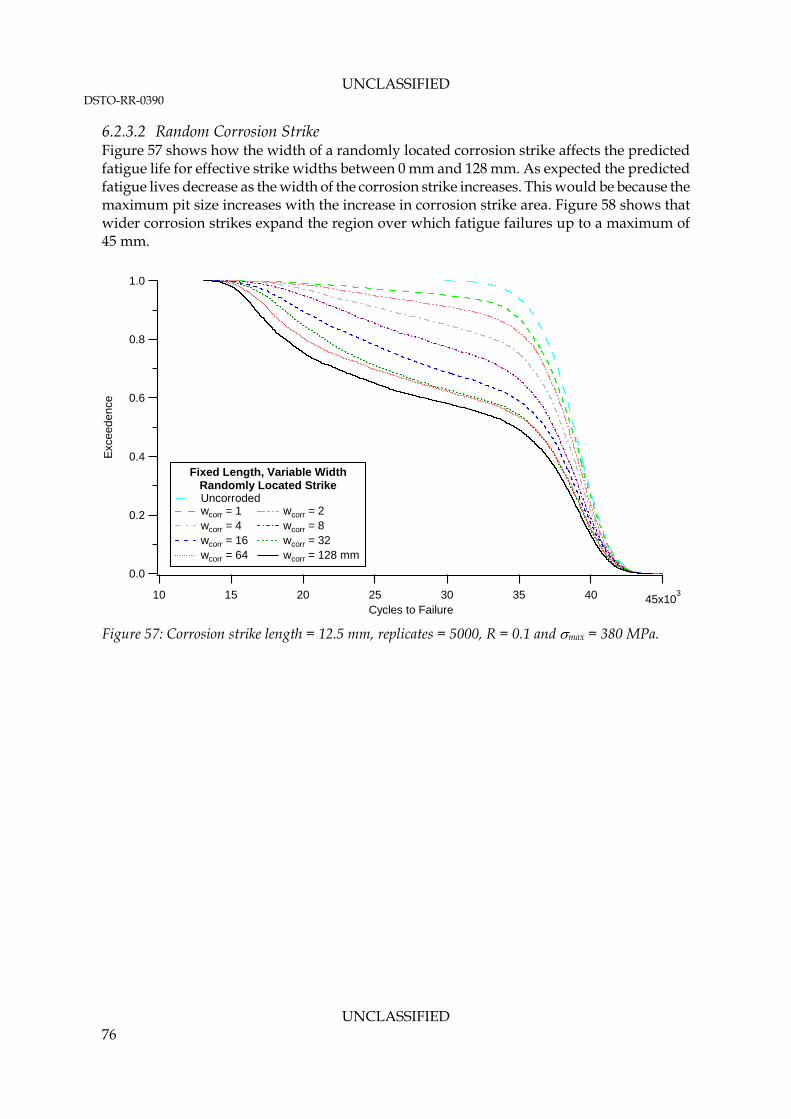
UNCLASSIFIED DSTO-RR-0390
UNCLASSIFIED 76
6.2.3.2 Random Corrosion Strike Figure 57 shows how the width of a randomly located corrosion strike affects the predicted fatigue life for effective strike widths between 0 mm and 128 mm. As expected the predicted fatigue lives decrease as the width of the corrosion strike increases. This would be because the maximum pit size increases with the increase in corrosion strike area. Figure 58 shows that wider corrosion strikes expand the region over which fatigue failures up to a maximum of 45 mm.
1.0
0.8
0.6
0.4
0.2
0.0
Exc
eed
ence
45x10340353025201510
Cycles to Failure
Fixed Length, Variable Width Randomly Located Strike Uncorroded wcorr = 1 wcorr = 2 wcorr = 4 wcorr = 8 wcorr = 16 wcorr = 32 wcorr = 64 wcorr = 128 mm
Figure 57: Corrosion strike length = 12.5 mm, replicates = 5000, R = 0.1 and max = 380 MPa.
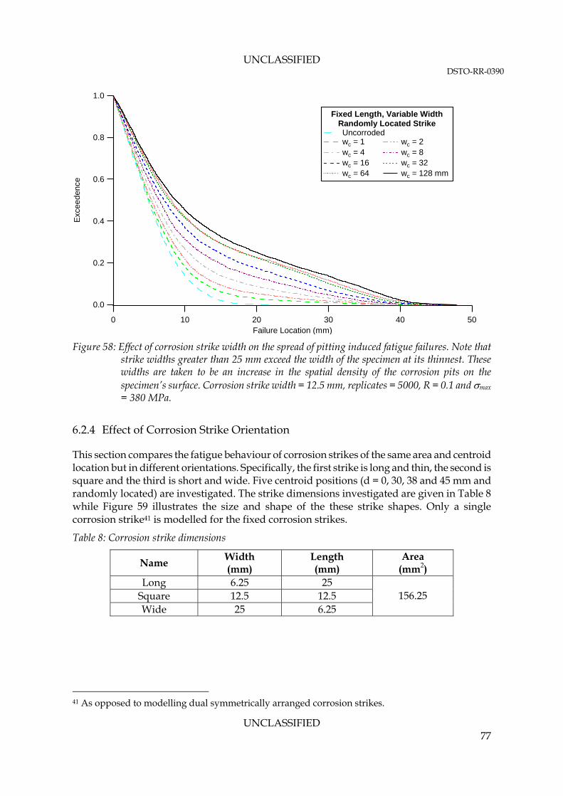
UNCLASSIFIED DSTO-RR-0390
UNCLASSIFIED 77
1.0
0.8
0.6
0.4
0.2
0.0
Exc
eed
ence
50403020100Failure Location (mm)
Fixed Length, Variable WidthRandomly Located Strike Uncorroded wc = 1 wc = 2 wc = 4 wc = 8 wc = 16 wc = 32 wc = 64 wc = 128 mm
Figure 58: Effect of corrosion strike width on the spread of pitting induced fatigue failures. Note that
strike widths greater than 25 mm exceed the width of the specimen at its thinnest. These widths are taken to be an increase in the spatial density of the corrosion pits on the specimen’s surface. Corrosion strike width = 12.5 mm, replicates = 5000, R = 0.1 and max = 380 MPa.
6.2.4 Effect of Corrosion Strike Orientation
This section compares the fatigue behaviour of corrosion strikes of the same area and centroid location but in different orientations. Specifically, the first strike is long and thin, the second is square and the third is short and wide. Five centroid positions (d = 0, 30, 38 and 45 mm and randomly located) are investigated. The strike dimensions investigated are given in Table 8 while Figure 59 illustrates the size and shape of the these strike shapes. Only a single corrosion strike41 is modelled for the fixed corrosion strikes.
Table 8: Corrosion strike dimensions
Name Width (mm)
Length (mm)
Area (mm2)
Long 6.25 25 Square 12.5 12.5 Wide 25 6.25
156.25
41 As opposed to modelling dual symmetrically arranged corrosion strikes.
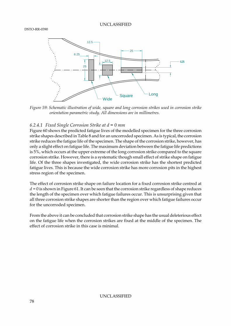
UNCLASSIFIED DSTO-RR-0390
UNCLASSIFIED 78
25
6.25
12.5
25
6.25
Long
12.5
Square Wide
Figure 59: Schematic illustration of wide, square and long corrosion strikes used in corrosion strike orientation parametric study. All dimensions are in millimetres.
6.2.4.1 Fixed Single Corrosion Strike at d = 0 mm Figure 60 shows the predicted fatigue lives of the modelled specimen for the three corrosion strike shapes described in Table 8 and for an uncorroded specimen. As is typical, the corrosion strike reduces the fatigue life of the specimen. The shape of the corrosion strike, however, has only a slight effect on fatigue life. The maximum deviation between the fatigue life predictions is 5%, which occurs at the upper extreme of the long corrosion strike compared to the square corrosion strike. However, there is a systematic though small effect of strike shape on fatigue life. Of the three shapes investigated, the wide corrosion strike has the shortest predicted fatigue lives. This is because the wide corrosion strike has more corrosion pits in the highest stress region of the specimen. The effect of corrosion strike shape on failure location for a fixed corrosion strike centred at d = 0 is shown in Figure 61. It can be seen that the corrosion strike regardless of shape reduces the length of the specimen over which fatigue failures occur. This is unsurprising given that all three corrosion strike shapes are shorter than the region over which fatigue failures occur for the uncorroded specimen. From the above it can be concluded that corrosion strike shape has the usual deleterious effect on the fatigue life when the corrosion strikes are fixed at the middle of the specimen. The effect of corrosion strike in this case is minimal.
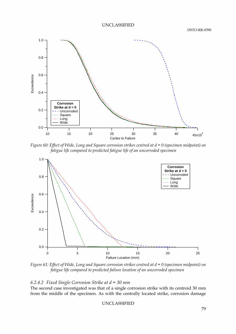
UNCLASSIFIED DSTO-RR-0390
UNCLASSIFIED 79
1.0
0.8
0.6
0.4
0.2
0.0
Exc
eede
nce
45x10340353025201510
Cycles to Failure
CorrosionStrike at d = 0
Uncorroded Square Long Wide
Figure 60: Effect of Wide, Long and Square corrosion strikes centred at d = 0 (specimen midpoint) on
fatigue life compared to predicted fatigue life of an uncorroded specimen
1.0
0.8
0.6
0.4
0.2
0.0
Exc
eed
ence
2520151050Failure Location (mm)
CorrosionStrike at d = 0
Uncorroded Square Long Wide
Figure 61: Effect of Wide, Long and Square corrosion strikes centred at d = 0 (specimen midpoint) on
fatigue life compared to predicted failure location of an uncorroded specimen
6.2.4.2 Fixed Single Corrosion Strike at d = 30 mm The second case investigated was that of a single corrosion strike with its centroid 30 mm from the middle of the specimen. As with the centrally located strike, corrosion damage
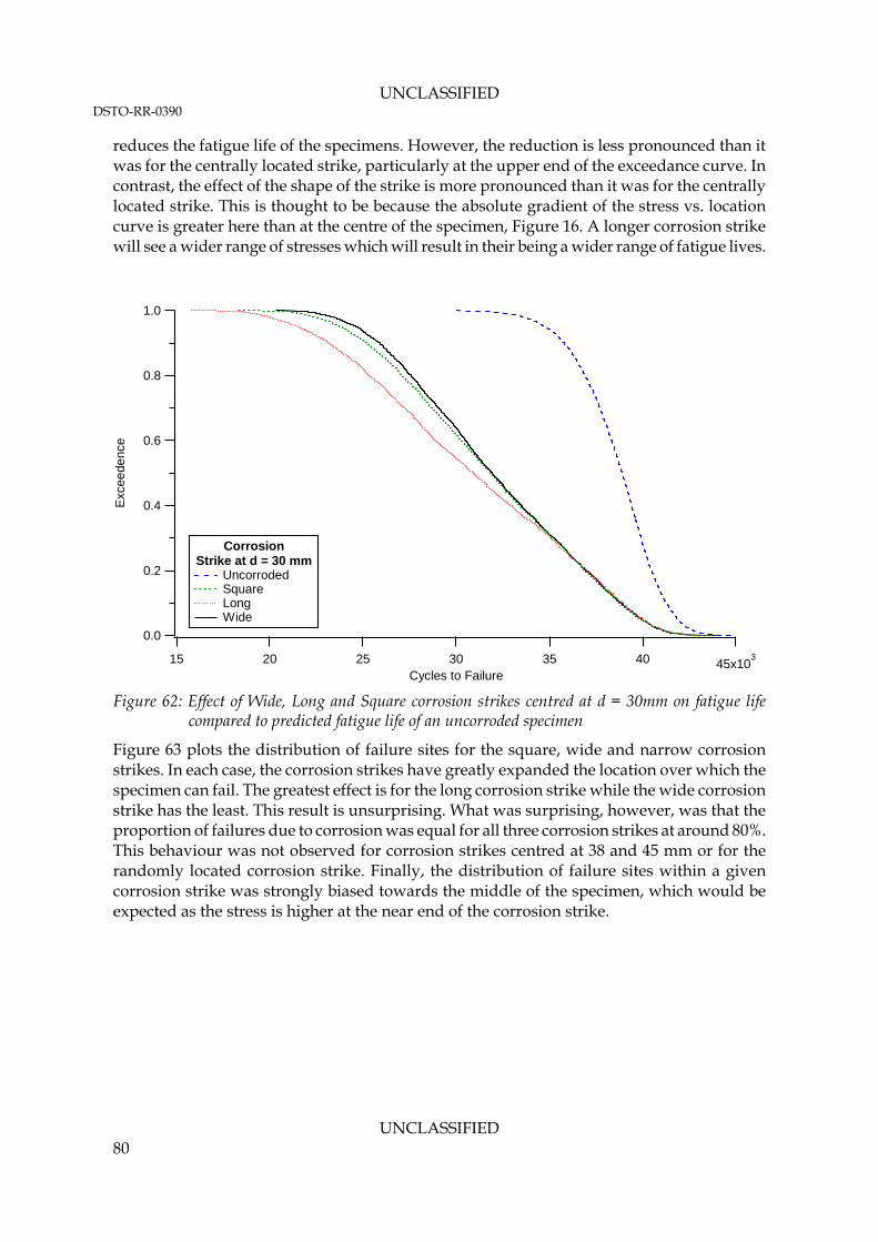
UNCLASSIFIED DSTO-RR-0390
UNCLASSIFIED 80
reduces the fatigue life of the specimens. However, the reduction is less pronounced than it was for the centrally located strike, particularly at the upper end of the exceedance curve. In contrast, the effect of the shape of the strike is more pronounced than it was for the centrally located strike. This is thought to be because the absolute gradient of the stress vs. location curve is greater here than at the centre of the specimen, Figure 16. A longer corrosion strike will see a wider range of stresses which will result in their being a wider range of fatigue lives.
1.0
0.8
0.6
0.4
0.2
0.0
Exc
eede
nce
45x103403530252015
Cycles to Failure
Corrosion Strike at d = 30 mm
Uncorroded Square Long Wide
Figure 62: Effect of Wide, Long and Square corrosion strikes centred at d = 30mm on fatigue life
compared to predicted fatigue life of an uncorroded specimen
Figure 63 plots the distribution of failure sites for the square, wide and narrow corrosion strikes. In each case, the corrosion strikes have greatly expanded the location over which the specimen can fail. The greatest effect is for the long corrosion strike while the wide corrosion strike has the least. This result is unsurprising. What was surprising, however, was that the proportion of failures due to corrosion was equal for all three corrosion strikes at around 80%. This behaviour was not observed for corrosion strikes centred at 38 and 45 mm or for the randomly located corrosion strike. Finally, the distribution of failure sites within a given corrosion strike was strongly biased towards the middle of the specimen, which would be expected as the stress is higher at the near end of the corrosion strike.
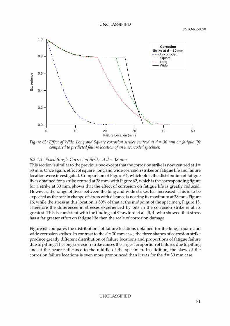
UNCLASSIFIED DSTO-RR-0390
UNCLASSIFIED 81
1.0
0.8
0.6
0.4
0.2
0.0
Exc
eed
ence
50403020100Failure Location (mm)
Corrosion Strike at d = 30 mm
Uncorroded Square Long Wide
Figure 63: Effect of Wide, Long and Square corrosion strikes centred at d = 30 mm on fatigue life
compared to predicted failure location of an uncorroded specimen
6.2.4.3 Fixed Single Corrosion Strike at d = 38 mm This section is similar to the previous two except that the corrosion strike is now centred at d = 38 mm. Once again, effect of square, long and wide corrosion strikes on fatigue life and failure location were investigated. Comparison of Figure 64, which plots the distribution of fatigue lives obtained for a strike centred at 38 mm, with Figure 62, which is the corresponding figure for a strike at 30 mm, shows that the effect of corrosion on fatigue life is greatly reduced. However, the range of lives between the long and wide strikes has increased. This is to be expected as the rate in change of stress with distance is nearing its maximum at 38 mm, Figure 16, while the stress at this location is 80% of that at the midpoint of the specimen, Figure 15. Therefore the differences in stresses experienced by pits in the corrosion strike is at its greatest. This is consistent with the findings of Crawford et al. [3, 4] who showed that stress has a far greater effect on fatigue life then the scale of corrosion damage. Figure 65 compares the distributions of failure locations obtained for the long, square and wide corrosion strikes. In contrast to the d = 30 mm case, the three shapes of corrosion strike produce greatly different distribution of failure locations and proportions of fatigue failure due to pitting. The long corrosion strike causes the largest proportion of failures due to pitting and at the nearest distance to the middle of the specimen. In addition, the skew of the corrosion failure locations is even more pronounced than it was for the d = 30 mm case.
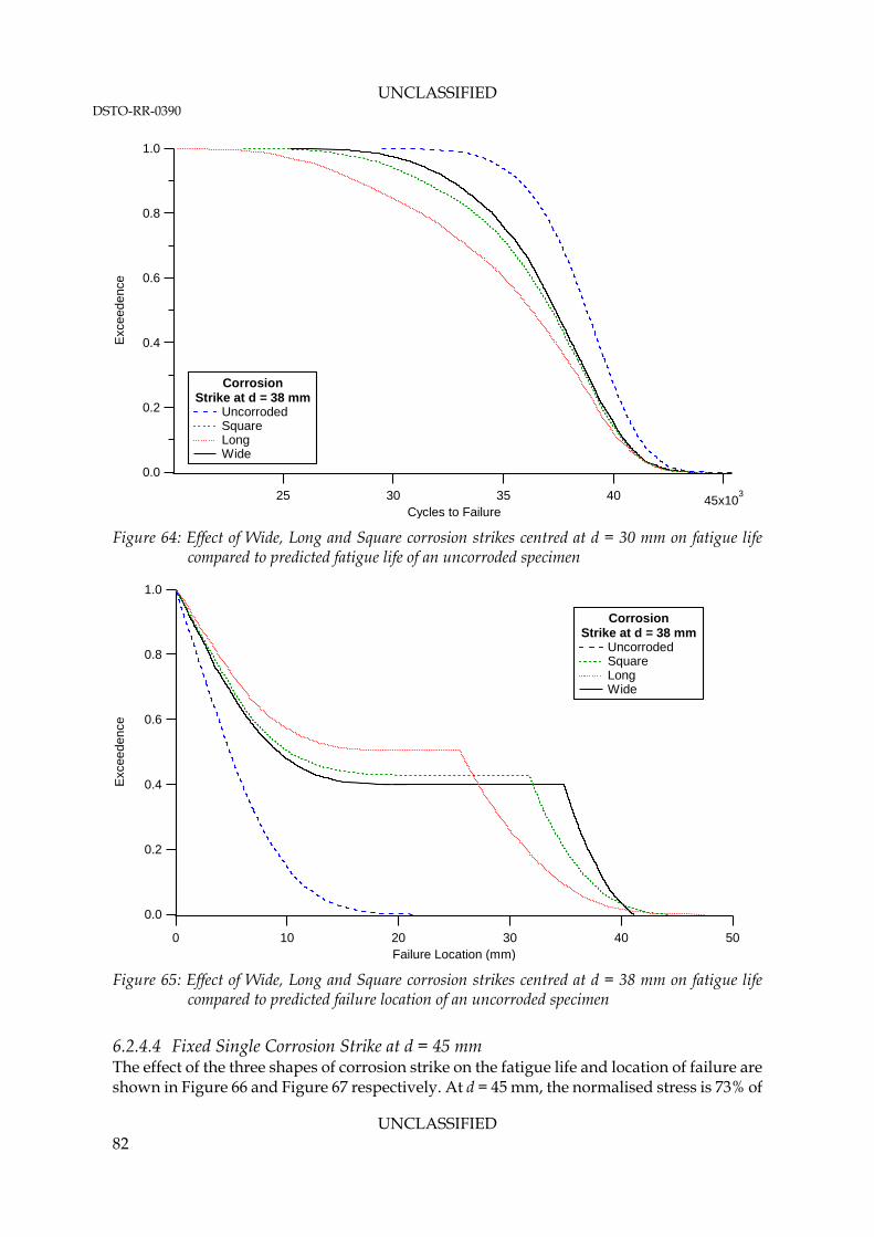
UNCLASSIFIED DSTO-RR-0390
UNCLASSIFIED 82
1.0
0.8
0.6
0.4
0.2
0.0
Exc
eede
nce
45x10340353025
Cycles to Failure
Corrosion Strike at d = 38 mm
Uncorroded Square Long Wide
Figure 64: Effect of Wide, Long and Square corrosion strikes centred at d = 30 mm on fatigue life
compared to predicted fatigue life of an uncorroded specimen
1.0
0.8
0.6
0.4
0.2
0.0
Exc
eed
ence
50403020100Failure Location (mm)
Corrosion Strike at d = 38 mm
Uncorroded Square Long Wide
Figure 65: Effect of Wide, Long and Square corrosion strikes centred at d = 38 mm on fatigue life
compared to predicted failure location of an uncorroded specimen
6.2.4.4 Fixed Single Corrosion Strike at d = 45 mm The effect of the three shapes of corrosion strike on the fatigue life and location of failure are shown in Figure 66 and Figure 67 respectively. At d = 45 mm, the normalised stress is 73% of
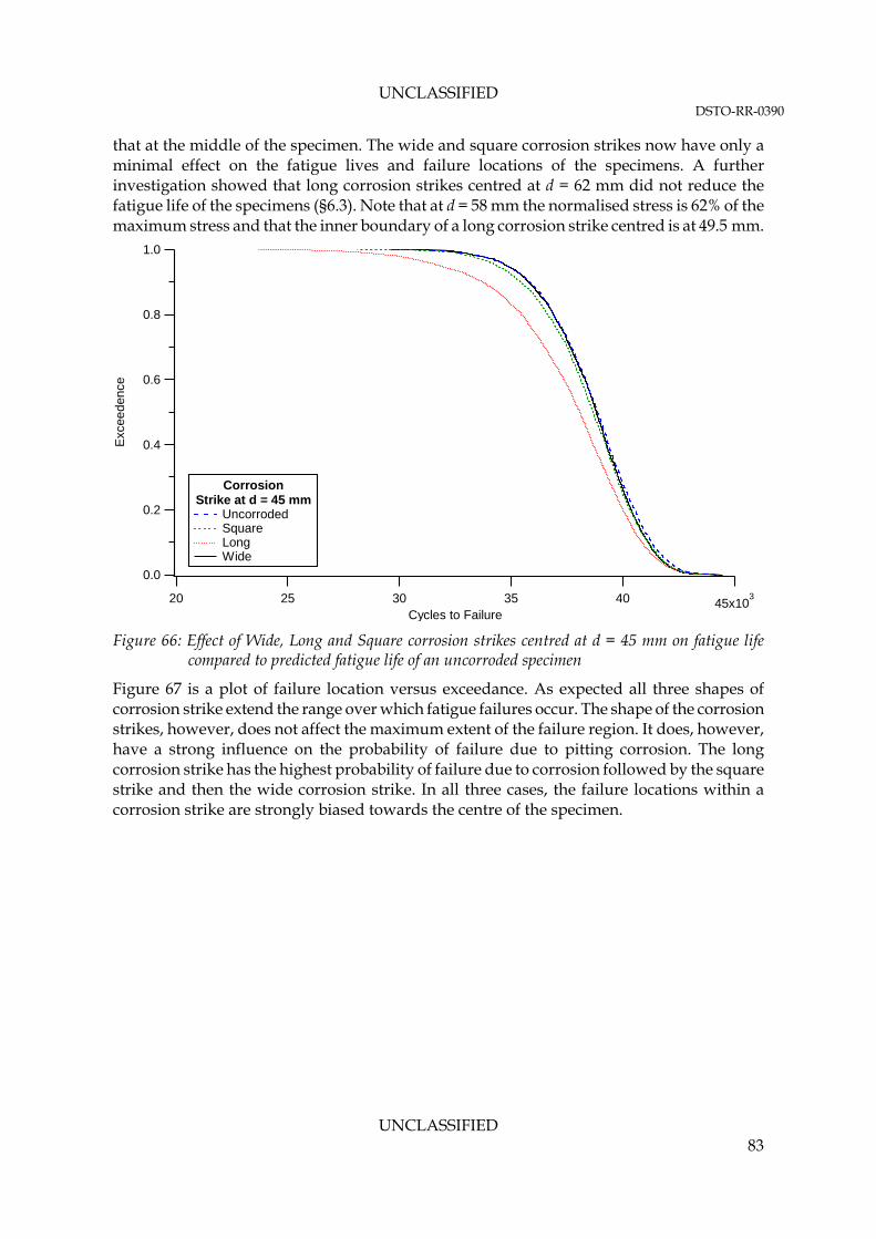
UNCLASSIFIED DSTO-RR-0390
UNCLASSIFIED 83
that at the middle of the specimen. The wide and square corrosion strikes now have only a minimal effect on the fatigue lives and failure locations of the specimens. A further investigation showed that long corrosion strikes centred at d = 62 mm did not reduce the fatigue life of the specimens (§6.3). Note that at d = 58 mm the normalised stress is 62% of the maximum stress and that the inner boundary of a long corrosion strike centred is at 49.5 mm.
1.0
0.8
0.6
0.4
0.2
0.0
Exc
eed
ence
45x1034035302520
Cycles to Failure
Corrosion Strike at d = 45 mm
Uncorroded Square Long Wide
Figure 66: Effect of Wide, Long and Square corrosion strikes centred at d = 45 mm on fatigue life
compared to predicted fatigue life of an uncorroded specimen
Figure 67 is a plot of failure location versus exceedance. As expected all three shapes of corrosion strike extend the range over which fatigue failures occur. The shape of the corrosion strikes, however, does not affect the maximum extent of the failure region. It does, however, have a strong influence on the probability of failure due to pitting corrosion. The long corrosion strike has the highest probability of failure due to corrosion followed by the square strike and then the wide corrosion strike. In all three cases, the failure locations within a corrosion strike are strongly biased towards the centre of the specimen.

UNCLASSIFIED DSTO-RR-0390
UNCLASSIFIED 84
1.0
0.8
0.6
0.4
0.2
0.0
Exc
eed
ence
50403020100Failure Location (mm)
Corrosion Strike at d = 45 mm
Uncorroded Square Long Wide
Figure 67: Effect of Wide, Long and Square corrosion strikes centred at d = 45 mm on fatigue life
compared to predicted failure location of an uncorroded specimen
6.2.4.5 Single Randomly Location Corrosion Strike Figure 68 shows that a randomly located corrosion strike of 156.25 mm2 area greatly reduces the predicted fatigue life of the model. This is particularly the case for the lower bound of the fatigue life. However, there is only a minor difference in fatigue life due to different shapes of the corrosion strike. The maximum difference between the fatigue life predictions is 9.3%. It can be concluded that the shape of a randomly located corrosion strike has only a minimal effect on fatigue life when the corrosion strike is randomly located. This means that it is acceptable to use a square corrosion strike of equal area for randomly located strikes. Figure 69 plots the predicted failure location for randomly located corrosion strikes. From this figure it is apparent that a randomly located corrosion strike can greatly increase the range of locations over which fatigue failure can occur. In this case the shape of the corrosion strike appears to have only minimal effect on failure location.

UNCLASSIFIED DSTO-RR-0390
UNCLASSIFIED 85
1.0
0.8
0.6
0.4
0.2
0.0
Exc
eede
nce
45x103403530252015
Cycles to Failure
Random Corrosion Strike
Uncorroded Square Long Wide
Figure 68: Effect of Wide, Long and Square randomly located corrosion strikes on fatigue life compared
to predicted fatigue life of an uncorroded specimen
1.0
0.8
0.6
0.4
0.2
0.0
Exc
eed
ence
50403020100Failure Location
Random Corrosion Strike
Uncorroded Square Long Wide
Figure 69: Effect of Wide, Long and Square randomly located corrosion strikes on fatigue life compared
to failure location of an uncorroded specimen
6.2.4.6 Summary of Strike Shape Effects From the above it is apparent that in many cases corrosion strike shape has only a minimal effect on fatigue life and failure location. The exceptions to this are when the stress field within the strike varies rapidly, such as near a fastener hole. In that case, a change in corrosion
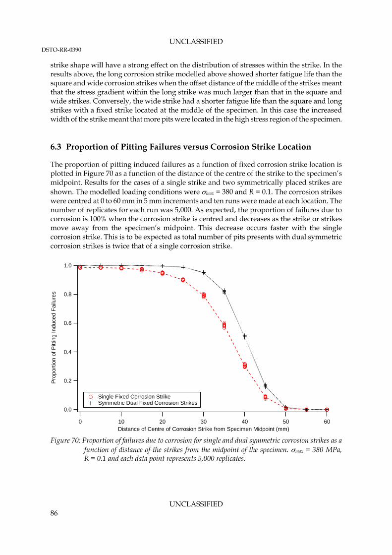
UNCLASSIFIED DSTO-RR-0390
UNCLASSIFIED 86
strike shape will have a strong effect on the distribution of stresses within the strike. In the results above, the long corrosion strike modelled above showed shorter fatigue life than the square and wide corrosion strikes when the offset distance of the middle of the strikes meant that the stress gradient within the long strike was much larger than that in the square and wide strikes. Conversely, the wide strike had a shorter fatigue life than the square and long strikes with a fixed strike located at the middle of the specimen. In this case the increased width of the strike meant that more pits were located in the high stress region of the specimen. 6.3 Proportion of Pitting Failures versus Corrosion Strike Location
The proportion of pitting induced failures as a function of fixed corrosion strike location is plotted in Figure 70 as a function of the distance of the centre of the strike to the specimen’s midpoint. Results for the cases of a single strike and two symmetrically placed strikes are shown. The modelled loading conditions were max = 380 and R = 0.1. The corrosion strikes were centred at 0 to 60 mm in 5 mm increments and ten runs were made at each location. The number of replicates for each run was 5,000. As expected, the proportion of failures due to corrosion is 100% when the corrosion strike is centred and decreases as the strike or strikes move away from the specimen’s midpoint. This decrease occurs faster with the single corrosion strike. This is to be expected as total number of pits presents with dual symmetric corrosion strikes is twice that of a single corrosion strike.
1.0
0.8
0.6
0.4
0.2
0.0
Pro
port
ion
of P
ittin
g In
duce
d F
ailu
res
6050403020100Distance of Centre of Corrosion Strike from Specimen Midpoint (mm)
Single Fixed Corrosion Strike Symmetric Dual Fixed Corrosion Strikes
Figure 70: Proportion of failures due to corrosion for single and dual symmetric corrosion strikes as a
function of distance of the strikes from the midpoint of the specimen. max = 380 MPa, R = 0.1 and each data point represents 5,000 replicates.
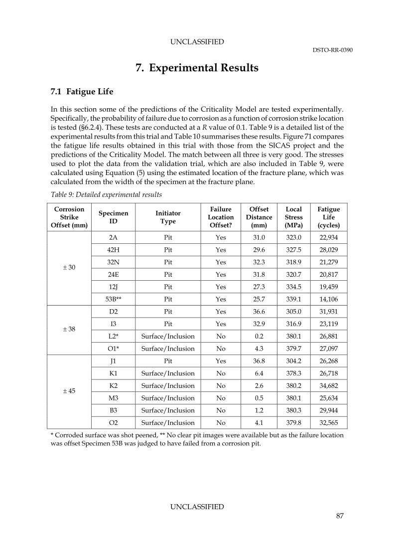
UNCLASSIFIED DSTO-RR-0390
UNCLASSIFIED 87
7. Experimental Results
7.1 Fatigue Life
In this section some of the predictions of the Criticality Model are tested experimentally. Specifically, the probability of failure due to corrosion as a function of corrosion strike location is tested (§6.2.4). These tests are conducted at a R value of 0.1. Table 9 is a detailed list of the experimental results from this trial and Table 10 summarises these results. Figure 71 compares the fatigue life results obtained in this trial with those from the SICAS project and the predictions of the Criticality Model. The match between all three is very good. The stresses used to plot the data from the validation trial, which are also included in Table 9, were calculated using Equation (5) using the estimated location of the fracture plane, which was calculated from the width of the specimen at the fracture plane.
Table 9: Detailed experimental results
Corrosion Strike
Offset (mm)
Specimen ID
Initiator Type
Failure Location Offset?
Offset Distance
(mm)
Local Stress (MPa)
Fatigue Life
(cycles)
2A Pit Yes 31.0 323.0 22,934
42H Pit Yes 29.6 327.5 28,029
32N Pit Yes 32.3 318.9 21,279
24E Pit Yes 31.8 320.7 20,817
12J Pit Yes 27.3 334.5 19,459
30
53B** Pit Yes 25.7 339.1 14,106
D2 Pit Yes 36.6 305.0 31,931
I3 Pit Yes 32.9 316.9 23,119
L2* Surface/Inclusion No 0.2 380.1 26,881 38
O1* Surface/Inclusion No 4.3 379.7 27,097
J1 Pit Yes 36.8 304.2 26,268
K1 Surface/Inclusion No 6.4 378.3 26,718
K2 Surface/Inclusion No 2.6 380.2 34,682
M3 Surface/Inclusion No 0.5 380.1 25,634
B3 Surface/Inclusion No 1.2 380.3 29,944
45
O2 Surface/Inclusion No 4.1 379.8 32,565
* Corroded surface was shot peened, ** No clear pit images were available but as the failure location was offset Specimen 53B was judged to have failed from a corrosion pit.
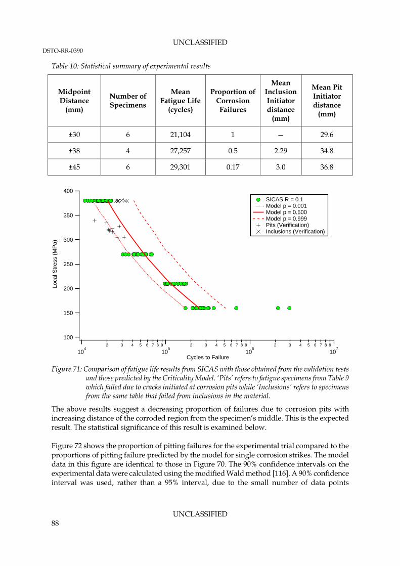
UNCLASSIFIED DSTO-RR-0390
UNCLASSIFIED 88
Table 10: Statistical summary of experimental results
Midpoint Distance
(mm)
Number of Specimens
Mean Fatigue Life
(cycles)
Proportion of Corrosion Failures
Mean Inclusion Initiator distance
(mm)
Mean Pit Initiator distance
(mm)
±30 6 21,104 1 — 29.6
±38 4 27,257 0.5 2.29 34.8
±45 6 29,301 0.17 3.0 36.8
400
350
300
250
200
150
100
Loca
l Str
ess
(MP
a)
104
2 3 4 5 6 7 8 9
105
2 3 4 5 6 7 8 9
106
2 3 4 5 6 7 8 9
107
Cycles to Failure
SICAS R = 0.1 Model p = 0.001 Model p = 0.500 Model p = 0.999 Pits (Verification) Inclusions (Verification)
Figure 71: Comparison of fatigue life results from SICAS with those obtained from the validation tests
and those predicted by the Criticality Model. ‘Pits’ refers to fatigue specimens from Table 9 which failed due to cracks initiated at corrosion pits while ‘Inclusions’ refers to specimens from the same table that failed from inclusions in the material.
The above results suggest a decreasing proportion of failures due to corrosion pits with increasing distance of the corroded region from the specimen’s middle. This is the expected result. The statistical significance of this result is examined below. Figure 72 shows the proportion of pitting failures for the experimental trial compared to the proportions of pitting failure predicted by the model for single corrosion strikes. The model data in this figure are identical to those in Figure 70. The 90% confidence intervals on the experimental data were calculated using the modified Wald method [116]. A 90% confidence interval was used, rather than a 95% interval, due to the small number of data points
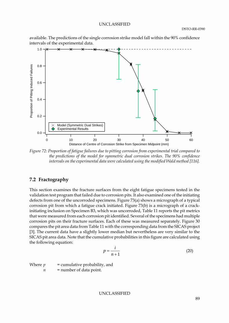
UNCLASSIFIED DSTO-RR-0390
UNCLASSIFIED 89
available. The predictions of the single corrosion strike model fall within the 90% confidence intervals of the experimental data.
1.0
0.8
0.6
0.4
0.2
0.0
Pro
port
ion
of P
ittin
g In
duce
d F
ailu
res
6050403020100Distance of Centre of Corrosion Strike from Specimen Midpoint (mm)
Model (Symmetric Dual Strikes) Experimental Results
Figure 72: Proportion of fatigue failures due to pitting corrosion from experimental trial compared to
the predictions of the model for symmetric dual corrosion strikes. The 90% confidence intervals on the experimental data were calculated using the modified Wald method [116].
7.2 Fractography
This section examines the fracture surfaces from the eight fatigue specimens tested in the validation test program that failed due to corrosion pits. It also examined one of the initiating defects from one of the uncorroded specimens. Figure 73(a) shows a micrograph of a typical corrosion pit from which a fatigue crack initiated. Figure 73(b) is a micrograph of a crack-initiating inclusion on Specimen B3, which was uncorroded, Table 11 reports the pit metrics that were measured from each corrosion pit identified. Several of the specimens had multiple corrosion pits on their fracture surfaces. Each of these was measured separately. Figure 30 compares the pit area data from Table 11 with the corresponding data from the SICAS project [3]. The current data have a slightly lower median but nevertheless are very similar to the SICAS pit area data. Note that the cumulative probabilities in this figure are calculated using the following equation:
1
n
ip (20)
Where p = cumulative probability, and n = number of data point.
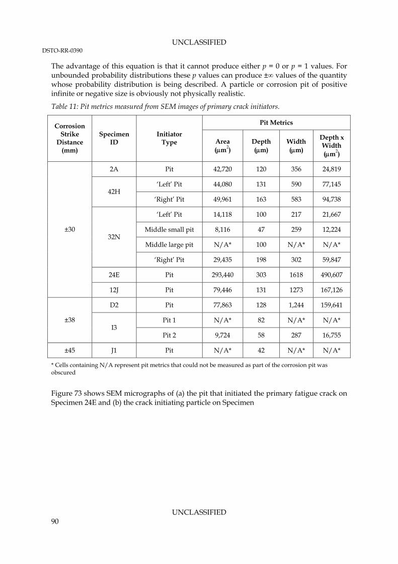
UNCLASSIFIED DSTO-RR-0390
UNCLASSIFIED 90
The advantage of this equation is that it cannot produce either p = 0 or p = 1 values. For unbounded probability distributions these p values can produce ±∞ values of the quantity whose probability distribution is being described. A particle or corrosion pit of positive infinite or negative size is obviously not physically realistic.
Table 11: Pit metrics measured from SEM images of primary crack initiators.
Pit Metrics Corrosion Strike
Distance (mm)
Specimen ID
Initiator Type Area
(m2) Depth (m)
Width (m)
Depth x Width (m2)
2A Pit 42,720 120 356 24,819
‘Left’ Pit 44,080 131 590 77,145 42H
‘Right’ Pit 49,961 163 583 94,738
‘Left’ Pit 14,118 100 217 21,667
Middle small pit 8,116 47 259 12,224
Middle large pit N/A* 100 N/A* N/A* 32N
‘Right’ Pit 29,435 198 302 59,847
24E Pit 293,440 303 1618 490,607
±30
12J Pit 79,446 131 1273 167,126
D2 Pit 77,863 128 1,244 159,641
Pit 1 N/A* 82 N/A* N/A* ±38 I3
Pit 2 9,724 58 287 16,755
±45 J1 Pit N/A* 42 N/A* N/A*
* Cells containing N/A represent pit metrics that could not be measured as part of the corrosion pit was obscured
Figure 73 shows SEM micrographs of (a) the pit that initiated the primary fatigue crack on Specimen 24E and (b) the crack initiating particle on Specimen
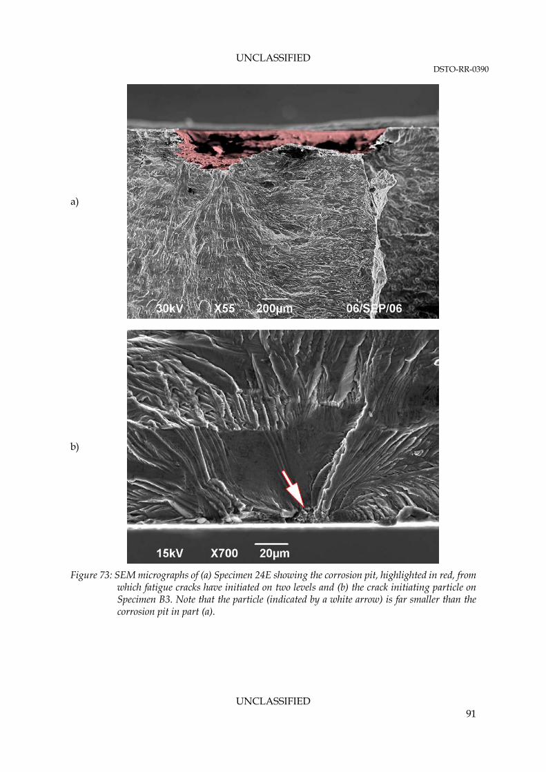
UNCLASSIFIED DSTO-RR-0390
UNCLASSIFIED 91
a)
b)
Figure 73: SEM micrographs of (a) Specimen 24E showing the corrosion pit, highlighted in red, from
which fatigue cracks have initiated on two levels and (b) the crack initiating particle on Specimen B3. Note that the particle (indicated by a white arrow) is far smaller than the corrosion pit in part (a).
UNCLASSIFIED DSTO-RR-0390
UNCLASSIFIED 92
8. Discussion
8.1 Summary of Results
This report has described a probabilistic model of how corrosion damage affects the initiation site of failure in the aluminium alloy 7010-T7651. This model used the low-kt fatigue life specimens used in the SICAS project [3, 4]. It is an empirical model based on corrosion pit and inclusion size data derived from the test material. It uses fatigue crack growth rate data obtained from a separate set of specimens of the same material and geometry. These data were used to create a fatigue life lookup table which returned a fatigue life to failure as a function of defect radius and local maximum stress. Stresses were calculated using a FE model of the fatigue specimens used. Comparison of the fatigue lives predicted by the model showed that they agreed extremely well with the fatigue life data obtained from the SICAS project at load ratios of -0.3, 0.1 and 0.5 for corroded specimens and 0.1 for the uncorroded material (§6.1.1). In the case of the corroded material (Figure 32 to Figure 34), the model produced good predictions of the mean value and scatter of the experimental fatigue lives whereas for the uncorroded material it was only able to predict the lower bound of the fatigue life (Figure 35). This latter observation was particularly apparent at lower stresses and is thought to be due to variability in the cycles required to initiate a fatigue crack from an inclusion.
The scatter in the model’s predictions was found to decrease linearly as a function of the inverse square root of the number of iterations (Figure 38), which is the behaviour expected from a Monte Carlo model. Based upon this convergence study it was decided to use 5,000 iterations for all subsequent modelling as this number of iterations gave the best balance between execution time and precision. The model was verified by comparing its fatigue life predictions with deterministic fatigue life predictions made using AFGROW (Figure 40). These were found to be in nearly exact agreement. However, at a maximum stress of 380 MPa and a R of 0.1, the predicted lives were slightly longer than the experimental lives from the SICAS project. Next, the effect of the area per defect was examined. It was found that the exceedance versus cycles to failure was not affected for corroded specimens between areas of 0.19 mm2 and 154 mm2 per defect42 (Figure 41). However, this was not the case for the uncorroded specimens which had a slightly faster decline in survival probability for an area per defect of 0.19 mm2 than for 154 mm2. A similar examination of the effect of maximum stress found that maximum stress had a negligible effect on the fatigue life predictions of the model (Figure 43). This is as expected given the assumption of purely Paris-law controlled fatigue crack growth. The model was also used to predict the effect of different size, shape, area and orientation of the corroded region on the fatigue life and failure location of the specimens (§6.2). These trials were further divided into trials using corrosion strikes of fixed location, typically centred at
42 Note that the area per defect of 0.19 mm2 was the base area for the extreme value distribution for the size of the inclusions while the area per defect value of 154 mm2 was the corresponding value for the corrosion pits.
UNCLASSIFIED DSTO-RR-0390
UNCLASSIFIED 93
the midpoint of the specimen, or randomly located along the length of the specimen’s reduced section. The study of the effect of corrosion strike length found that fixed corrosion strikes actually decreased the spread of fatigue failures (Figure 50). The main effect of fixed, centrally-located (d = 0) corrosion strikes was to reduce the fatigue endurance of the specimen. In contrast, randomly located corrosion strikes increased the spread of fatigue failure locations and reduced the fatigue endurance of the specimens. The reduction in fatigue life due to randomly located corrosion strikes was less than that for a fixed corrosion strike of the same length and width. The effect of strike width was studied using a corrosion strike of constant length (12.5 mm) and a width varying from 0 mm (uncorroded) to 128 mm. Corrosion strike widths greater than 25 mm, the minimum width of the specimen, were considered to be an increase in the spatial density of the corrosion pits. Fixed corrosion strikes were centred at the middle of the specimen while random corrosion strikes were allowed to occur anywhere along the reduced section of the specimen. The effect of corrosion strike width for a fixed corrosion strike was similar to that for corrosion strike length (Figure 52). Specifically, a corrosion strike at the middle of the specimen decreases the fatigue endurance of the specimen while decreasing the spread of failure locations. Randomly located corrosion strikes increase the spread of fatigue failures for except for when the corrosion strike is 128 mm wide at which point the spread of failure locations is reduced. A special trial was conducted with single and dual symmetric corrosion strikes at 5 mm increments from the specimen’s midpoint (Figure 70). These corrosion strikes were square with an area of 156.25 mm2. The proportion of failures due to pitting was found to decrease sigmoidally as a function of increasing distance of the corrosion strikes from the middle of the specimen. The decrease occurred at slightly lower values for the dual strikes case than for the single strike case. In addition to modelling, an experimental trial of 16 corroded low-kt specimens of the same geometry was conducted. The predictions of the model were compared with these experimental results (Figure 71). The location of the failure point of each specimen was measured and a local stress was calculated from this value. These fatigue life results agreed well with the experimental results from SICAS and the predictions made by the model. This was true of specimens that failed due to cracks initiated from corrosion pits and for those that failed from cracks initiated at inclusions. The observed proportion of pitting failures as a function of the corrosion strike location was also a good match to the predictions of the model (Figure 72). The model’s predictions fell within the 90% confidence interval of the experimental data. Fractographic examination of the specimens showed that the width, depth and area of the pits on these specimens were within the size distributions observed in the SICAS project [3, 4]. 8.2 Comparison with the Literature
8.2.1 Fatigue Life Predictions
As discussed in §2.5, there have been numerous attempts to predict the fatigue life of aluminium alloys over the last few decades. In §2.5.3 we briefly reviewed models from Alcoa
UNCLASSIFIED DSTO-RR-0390
UNCLASSIFIED 94
Technical Center, the National Research Council of Canada , the University of Utah, Cornell University, Purdue University, The University of Virginia and The Norwegian University of Science and Technology. Magnusen et al. [46, 47] of Alcoa Technical Center found that their model made excellent predictions of the fatigue life of uncorroded early (pre-1984) and late (post-1984) manufacture-date 7050-T7451 using low-kt fatigue specimen. In contrast their model underestimated the fatigue life of low-kt specimens of the low porosity 7050-T7451 they examined. High-kt fatigue life tests using open hole specimens produced a somewhat different result. The fatigue lives of the early, late and low-porosity variant materials were accurately predicted while the fatigue life of a thin 7050-T7451 variants was overestimated. Comparison of Figure 4 with Figure 32 to Figure 35 shows that the fatigue predictions of the Magnusen et al. were of similar quality to those of the current work. In contrast to the current work, however, Magnusen et al. [47] used fatigue crack growth data from long crack growth specimens. This suggests that good quality fatigue crack growth data can give good predictions of fatigue life under constant amplitude conditions as long as modelling is conducted carefully. The fatigue life predictions of Fjeldstad et al. [24] were also of similar accuracy to those of Magnusen and those in the current work. 8.2.2 Failure Location Prediction
As discussed in the §2.3, very little work has been published on how corrosion damage affects the location of fatigue failures in aircraft. The clearest comparison is with Cook et al. [21] who examined the effect of surface corrosion around cold expanded holes in high-kt specimens of 7050-T76. However, the current work was conducted on low-kt specimens and is therefore not directly comparable. Karlén et al. [103] noted that the predicted locations of fatigue failures in low-kt specimens of Weldox 420 steel were more diffuse and penetrated more deeply into the cross-section of the specimens than for high-kt specimens of the same material. They attributed this difference to the shallower stress gradient of the low-kt specimens. As the current work concentrated solely on surface defects in low-kt specimens it was not possible to confirm or disprove this observation. 8.3 Significance of Results
The purpose of this report was to investigate the hypothesis that pitting corrosion can increase the area over which fatigue failures can occur in aircraft structures. This investigation was undertaken using a Monte Carlo model of an idealised fatigue life coupon combined with experimental data from fatigue tests of real coupons of the same geometry. It was found for this specimen that pitting corrosion greatly increased the areas over which fatigue failures could occur. For example, isolated regions of pitting, herein called ‘corrosion strikes’, could cause fatigue failures at locations distant from the nominally critical region of the specimen. In the safety-by-inspection airworthiness philosophy fatigue critical regions of aircraft are identified from analysis, teardowns and full scale fatigue tests or from in-service failures. None of these methods of identifying fatigue critical regions, other than in-service failures, accounts for the effects of in-service corrosion on structural integrity. As a result in-service corrosion damage could lead to the failure of unexpected components or failures in
UNCLASSIFIED DSTO-RR-0390
UNCLASSIFIED 95
unexpected locations in fatigue critical components. The in-service failure of TEF lugs in the F/A-18 [13] demonstrates that the feasibility of the first of these cases while the model developed in this report supports the feasibility of the second case. The model has also shown a means of predicting and dealing with unexpected failures from corrosion damage. In the current case corrosion damage was modelled as either a single randomly located corrosion strike of set area or as a corrosion strike of set area at a set location. This is not likely to be the case in service and the model could readily be modified to deal with multiple corrosion strikes. The model could also be further generalised to work on components of arbitrary shape rather than the very simple geometry examined in this report.
9. Conclusions and Further Work
This report has described the development and validation and verification of a Monte Carlo model of the effect of pitting corrosion on the fatigue life and failure locations of a simple low-kt fatigue specimen. The fatigue life predictions of this model agreed very well with the experimental fatigue life data from the SICAS project. A small experimental study using specimens of this geometry was then conducted to test the model’s predictions of the effect of corrosion on fatigue failure locations. The results of the experimental study agreed well with the model’s predictions. Given the success of the model it is recommended that the following future work should be pursued to fully exploit the model’s capabilities:
1. Fatigue crack growth data similar to the MB dataset from SICAS [3, 4] used in this report should be collected for extruded 7050-T7451 and perhaps 7075-T6 and incorporated into the model.
2. The model and experimental trial should be repeated under variable amplitude loading conditions. Ideally, this would be for 7050-T7451 and 7075-T6 due to the use of these alloys on RAAF aircraft using loading spectra representative of RAAF usage.
3. Variants of the model should be created for more complex geometries than the effectively one-dimensional low-kt geometry investigated in this report. Suggested variants include:
a. A single hole high-kt fatigue coupons such as that used by Crawford and Sharp [22]. An experimental plan along these lines has already been developed and published as Crawford et al. [117].
b. A three hole high-kt specimen based on the one hole high-kt specimen used by Crawford and Sharp [22].
c. A model that simulates a section of a real aircraft component such as the fuel flow vent holes in the F-111 wing pivot fitting. These have previously been examined by Mills et al. [67].
d. A multi-site damage model such as that developed by Burchill for an F-111 wing [96].
e. A model for arbitrary shaped components such as that developed by Wormsen et al. [25] for uncorroded steel components. This variant should also allow the
UNCLASSIFIED DSTO-RR-0390
UNCLASSIFIED 96
modelling of multiple arbitrarily shaped corrosion strikes on any shape component.
f. A model for the effect of corrosion on lap-joints.
4. The model should be combined with a pitting corrosion prediction model to allow end-to-end prediction of the incidence of pitting corrosion damage and its effect on aircraft structural integrity. The pitting model developed by Trueman of DSTO is a candidate for this.
10. Acknowledgements
The authors would like to thank:
Steve Sanderson of DSTO for his help with FE analysis.
Claude Urbani of CSIRO for the FE model of the low-kt fatigue specimen used in this work.
Noel Goldsmith of DSTO for his assistance with fractography and optical microscopy.
Rohan Byrnes of DSTO for assistance with specimen preparation for the SEM microscope and examination of the specimens prepared.
Dr Simon Barter of DSTO for his advice regarding the quantitative fractography methods which were used to collect the fatigue crack growth data used in this report.
Dr Tony Trueman and Kayne Begbie for advice on how to corrode the test specimens.
Carlos Rey, Bruce Crosbie and Rodney Grey of the DSTO fatigue testing laboratory for their assistance with the fatigue testing described in this report.
Professor Graham Clark, formerly of DSTO, for suggesting the original concept of corrosion criticality.
Dr Min Liao of the National Research Council of Canada for his careful review of this report.

UNCLASSIFIED DSTO-RR-0390
UNCLASSIFIED 97
11. References
1. Crawford, B. R., Loader, C. and Sharp, P. K. (2010) A Proposed Roadmap for Transitioning DSTO's Corrosion Structural Integrity Research into Australian Defence Force Service. DSTO-TR-2475, [Technical Report] Melbourne, Defence Science and Technology Organisation
2. ASTM (2002) E466-96(2002)e1 Standard Practice for Conducting Force Controlled Constant Amplitude Axial Fatigue Tests of Metallic Materials. In: ASTM Annual Book of Standards. Vol. 03.01. ASTM
3. Crawford, B. R., Loader, C., Sharp, P. K., Clark, G., Urbani, C., Hay, D., Ward, A., Bache, M., Evans, W. J., Stonham, A. ,Spence, S. (2005) Structural Integrity Assessment of Corrosion in Aircraft Structures. DSTO-RR-0294, Melbourne, DSTO
4. Crawford, B. R., Loader, C., Ward, A. R., Urbani, C., Bache, M. R., Spence, S. H., Hay, D. G., Evans, W. J., Clark, G. and Stonham, A. J. (2005) The EIFS distribution for anodised and pre-corroded 7010-T7651 under constant amplitude loading. Fatigue and Fracture of Engineering Materials and Structures 28 (9) 795-808
5. Castillo, E. (1988) Extreme Value Theory in Engineering. Statistical Modeling and Decision Science, Lieberman, G. and Olkin, I. ed. Vol. 1. San Diego, Academic Press
6. Watters, K., Rose, F., Heller, M., Callus, P., Madley, B. and Connor, P. (2001) F-111 Sole Operator Program: Maintaining the Structural Integrity of an Ageing Fighter Aircraft. In: RTO AVT Specialists’ Meeting on Life Management Techniques for Ageing Air Vehicles, Manchester, UK: 8-11 October 2001, RTO-AVT
7. Wikipedia. F-111 Aardvark Operators. (2012) [Accessed 2012 23/11/2012]; Available from: http://en.wikipedia.org/wiki/General_Dynamics_F-111_Aardvark#Operators.
8. Tiffany, C. F., Gallagher, J. P. and Babish IV, C. A. (2010) Threats to Aircraft Structural Safety, Including a Compendium of Selected Structural Accidents / Incidents. ASC- TR-2010-5002, [Final Report] Wright Patterson Air Force Base, OH 45433-7101, USA, USAF
9. Wikipedia. Boeing B-52 Stratofortress. (2012) [Accessed 2012 23/11/12]; Available from: http://en.wikipedia.org/wiki/B52.
10. Kinzie, R. C. (2002) USAF Cost of Corrosion Maintenance. In: Sixth Joint FAA/DoD/NASA Conference on Aging Aircraft, San Francisco CA, USA: 16-19th September 2002, FAA/DoD/NASA
11. Hoeppner, D. W., Grimes, L., Hoeppner, J., Ledesma, T., Mills, T. and Shah, A. (1995) Corrosion and Fretting as Critical Aviation Safety Issues. In: International Congress on Aircraft Fatigue,
12. Aircraft Accident Report - Aloha Airlines, Flight 243, Boeing 737-200. (1989) NTSB/AAR-89/03, Washington, National Transportation Safety Board
13. Barter, S. A., Sharp, P. K. and Clark, G. (1994) The failure of an F/A-18 trailing edge flap hinge. Engineering Failure Analysis 1 (4) December 1994 255-266
UNCLASSIFIED DSTO-RR-0390
UNCLASSIFIED 98
14. Budnick, J. (2003) NAVAIR Air Vehicle Corrosion Challenges. In: Tri-Service Corrosion Conference, Las Vegas: 17 –21 November 2003, US Department of Defence
15. Peeler, D. T. and Kinzie, R. C. (2001) Corrosion damage management and future outlook on corrosion prediction tools. In: 5th Joint FAA/DoD/NASA Conference on Aging Aircraft, Kissimmee, FL, USA: September 10-13, 2001
16. Brooks, C. L., Prost-Domasky, S. and Honeycutt, K. (1998) Corrosion is a Structural and Economic Problem: Transforming Metrics to a Life Prediction Method. In: NATO RTO’s Workshop 2 on Fatigue in the Presence of Corrosion, Corfu, Greece,: 7-8 October 1998, NATO
17. Cole, G. K., Clark, G. and Sharp, P. K. (1997) The implications of corrosion with respect to aircraft structural integrity. DSTO-RR-0102, [Research Report] Melbourne, DSTO
18. Hinton, B. R. W., Trathen, P., Duxbury, E., Salagaras, M. and Bushell, P. (2001) The Protection Performance of Corrosion Prevention Compounds on Aluminium Alloys in Laboratory and Outdoor Environments. In: DOD/FAA/NASA 5th Aging Aircraft Conference, Orlando FL, USA
19. ASTM (2013) E647-13 Standard Test Method for Measurement of Fatigue Crack Growth Rates In: ASTM Annual Book of Standards. Vol. 03.01. Philadelphia, PA, USA, ASTM
20. Clark, G. (1999) Management of Corrosion in Aging Military Systems. In: RTO AVT Specialists Meeting on Life Management Techniques for Ageing Air Vehicles. Manchester, UK, NATA Research and Technology Organisation
21. Cook, R., Blinos, N. and Wagstaff, P. (1998) Role of Surface Corrosion on Effectiveness of Hole Cold Expansion. In: Fatigue in the Presence of Corrosion, Corfu, Greece: 7-8 October, RTO
22. Crawford, B. R. and Sharp, P. K. (2012) Equivalent Crack Size Modelling of Corrosion Pitting in an AA7050-T7451 Aluminium Alloy and its Implications for Aircraft Structural Integrity. DSTO-TR-2745, [Technical Report] Melbourne, DSTO
23. Mills, T. and Honeycutt, K. T. (2011) Holistic Structural Integrity Analysis for Corrosion in a Hub on a Transport Aircraft Frame. In: Corrosion Fatigue and Environmentally Assisted Cracking in Aging Military Vehicles. Neuilly-Sur-Seine Cedex, France, NATO-RTO
24. Fjeldstad, A., Wormsen, A. and Härkegård, G. (2008) Simulation of fatigue crack growth in components with random defects. Engineering Fracture Mechanics 75 1187-1203
25. Wormsen, A., Fjeldstad, A. and Härkegård, G. (2008) A post-processor for fatigue crack growth analysis based on a finite element stress field. Computational Methods in Applied Mechanical Engineering 197 834-845
26. Future Airframe Structural Lifing: Methods, Applications and Management. (2009) TR-AVT-125, North Atlantic Treaty Organisation - Research And Technology Organisation
27. Miner, M. A. (1945) Cumulative Damage in Fatigue. Journal of Applied Mechanics 12 159-164
UNCLASSIFIED DSTO-RR-0390
UNCLASSIFIED 99
28. Frost, N. E. and Dugdale, D. S. (1958) The propagation of fatigue cracks in sheet specimens. Journal of the Mechanics and Physics of Solids 6 (2) 92-110
29. Bozek, J. E., Hochhalter, J. D., Veilleux, M. G., Liu, M., Heber, G., Sintay, S. D., Rollett, A. D., Littlewood, D. J., Maniatty, A. M., Weiland, H., Christ, R. J., Payne, J., Welsh, G., Harlow, D. G., Wawrzynek, P. A. ,Ingraffea, A. R. (2008) A geometric approach to modeling microstructurally small fatigue crack formation: I. Probabilistic simulation of constituent particle cracking in AA 7075-T651. Modelling and Simulation in Materials Science and Engineering 16 (6)
30. Hochhalter, J. D., Littlewood, D. J., Christ, R. J., Veilleux, M. G., Bozek, J. E., Ingraffea, A. R. and Maniatty, A. M. (2010) A geometric approach to modeling microstructurally small fatigue crack formation: II. Physically based modeling of microstructure-dependent slip localization and actuation of the crack nucleation mechanism in AA 7075-T651. Modelling and Simulation in Materials Science and Engineering 18 (4)
31. Hochhalter, J. D., Littlewood, D. J., Veilleux, M. G., Bozek, J. E., Maniatty, A. M., Rollett, A. D. and Ingraffea, A. R. (2011) A geometric approach to modeling microstructurally small fatigue crack formation: III. Development of a semi-empirical model for nucleation. Modelling and Simulation in Materials Science and Engineering 19 (3)
32. Tuegel, E. J., Ingraffea, A. R., Eason, T. G. and Spottswood, S. M. (2011) Reengineering aircraft structural life prediction using a digital twin. International Journal of Aerospace Engineering 2011 (Article ID 154798) 14 pages
33. White, P. (2011) Molecular dynamics of fatigue crack growth. In: DSTO-AVD Seminar, Melbourne: November 9th, 2011, DSTO
34. Paris, P. C., Gomez, M. P. and Anderson, W. P. (1961) A rational analytic theory of fatigue. The Trend in Engineering 13 9-14
35. Forman, R. G., Kearney, V. E. and Engle, R. M. (1967) Numerial analysis of crack propagation in cyclic-loaded structures. Journal of Basic Engineering 89 459-464
36. NASGRO. (2003) [Accessed 10/4/2013]; Available from: http://www.swri.edu/4org/d18/mateng/matint/NASGRO/default.htm.
37. Walker, K. (1970) The effect of stress ratio during crack propagation and fatigue for 2024-T3 and 7075-T6 aluminum. In: Effects of Environment and Complex Loading History for Fatigue Life. Philadelphia, American Society of Testing and Materials 1-14
38. Harter, J. AFGROW Program. (2003) [Accessed 07/01/2008]; Available from: http://www.siresearch.info/projects/afgrow/downloads/afgrow/a_v4-11-14.exe.
39. Newman Jr., J. C. (1992) FASTRAN II - a fatigue crack growth structural analysis program. NASA TM 104159,
40. Wallbrink, C. and Hu, W. (2010) A Strain-Life Module for CGAP: Theory, User Guide and Examples. DSTO-TR-2392, Melbourne, DSTO
41. Suresh, S. (1991) Fatigue of Materials. 1st ed. Cambridge Solid State Science Series, Davis, E. A. and Ward, I. M. ed. Cambridge UK, Cambridge University Press
UNCLASSIFIED DSTO-RR-0390
UNCLASSIFIED 100
42. Crawford, B. R. (1986) Fatigue of an Al-6061 matrix composite. [Doctorate of Philosophy] Brisbane, University of Queensland
43. Inglis, C. E. (1913) Stresses in a plate due to the presence of cracks and sharp corners. Transactions of the Institute of Naval Architects 55 219-241
44. Irwin, G. R. (1957) Analysis of stresses and strains near the end of a crack traversing a plate. Journal of Applied Mechanics 24 361-364
45. Hu, W., Tong, Y. C., Walker, K. F., Mongru, D., Amaratunga, R. and Jackson, P. (2006) A Review and Assessment of Current Airframe Lifiing Methodologies an Tools in Air Vehicles Division. DSTO-RR-0321, [Research Report] Melbourne, DSTO
46. Magnusen, P. E., Bucci, R. J., Hinkle, A. J., Brockenbrough, J. R. and Konish, H. J. (1997) Analysis and prediction of microstructural effects on long-term fatigue performance of an aluminum aerospace alloy. International Journal of Fatigue 19 (Supplement 1) S275-S283
47. Magnusen, P. E., Bucci, R. J., Hinkle, A. J., Brockenbrough, J. R., Konish, H. J. and Miyasato, S. M. (1996) Final Report: The Role of Microstructure on the Fatigue Durability of Aluminum Aircraft Alloys. [Final Report] Arlington, VA, Alcoa Technical Center
48. Przystupa, M. A., Bucci, R. J., Magnusen, P. E. and Hinkle, A. J. (1997) Microstructure based fatigue life predictions for thick plate 7050-T7451 airframe alloys. International Journal of Fatigue 19 (SUPPL.1) S285-S288
49. Liao, M., Renaud, G. and Bellinger, N. C. (2007) Fatigue modeling for aircraft structures containing natural exfoliation corrosion. International Journal of Fatigue 29 (4) 677-686
50. Jones, K. and Hoeppner, D. W. (2005) Pit-to-crack transition in pre-corroded 7075-T6 aluminum alloy under cyclic loading. Corrosion Science 47 (9) 2185-2198
51. Mills, T. B., Honeycutt, K. T., Brooks, C. L., Sharp, P. K., Loader, C. and Crawford, B. R. (2004) Development and Demonstration of an Holistic Structural Integrity Process using the Initial Discontinuity State Concept for 7050-T7451 Aluminum. Analytical Processes Engineered Solutions
52. Shekhter, A., Loader, C., Hu, W. and Crawford, B. R. (2007) Assessment of the effect of pitting corrosion on the safe life prediction of the P3-C. DSTO-TR-2080, [Technical Report] Defence Science and Technology Organisation
53. Debartolo, E. A. and Hillberry, B. M. (2004) Predicting fatigue life under spectrum loading in 2024-T3 aluminium using a measured initial flaw size distribution. ASTM Special Technical Publication (1450) 75-86
54. Gruenberg, K. M., Craig, B. A., Hillberry, B. M., Bucci, R. J. and Hinkle, A. J. (2004) Predicting fatigue life of pre-corroded 2024-T3 aluminum. International Journal of Fatigue 26 (6) 629-640
55. Laz, P. J., Craig, B. A. and Hillberry, B. M. (2001) A probabilistic total fatigue life model incorporating material inhomogeneities, stress level and fracture mechanics. International Journal of Fatigue 23 (Supplement 1) S119-S127
56. Laz, P. J. and Hillberry, B. M. (1998) Fatigue life prediction from inclusion initiated cracks. International Journal of Fatigue 20 (4) 263-270
UNCLASSIFIED DSTO-RR-0390
UNCLASSIFIED 101
57. van der Walde, K. and Hillberry, B. M. (2008) Characterization of pitting damage and prediction of remaining fatigue life. International Journal of Fatigue 30 (1) 106-118
58. Zamber, J. E. and Hillberry, B. M. (1999) Probabilistic approach to predicting fatigue lives of corroded 2024-T3. AIAA journal 37 (10) 1311-1317
59. Burns, J. T., Kim, S. and Gangloff, R. P. (2010) Effect of corrosion severity on fatigue evolution in Al–Zn–Mg–Cu. Corrosion Science 52 498-508
60. Burns, J. T., Larsen, J. M. and Gangloff, R. P. (2011) Driving forces for localized corrosion-to-fatigue crack transition in Al–Zn–Mg–Cu. Fatigue and Fracture of Engineering Materials and Structures 34 745-773
61. Payne, J., Welsh, G., Christ Jr, R. J., Nardiello, J. and Papazian, J. M. (2010) Observations of fatigue crack initiation in 7075-T651. International Journal of Fatigue 32 (2) 247-255
62. Schumacher, J., Bomas, H. and Zoch, H. W. (2012) Endurance limit prediction for sulphur-alloyed spray-formed steels. International Journal of Fatigue 41 119-129
63. Papazian, J. M., Anagnostou, E. L., Engel, S. J., Hoitsma, D., Madsen, J., Silberstein, R. P., Welsh, G. and Whiteside, J. B. (2009) A structural integrity prognosis system. Engineering Fracture Mechanics 76 620-632
64. Aircraft Structural Integrity Program: Airplane Requirements. (1972) MIL-STD-1530, (US) Department of Defence
65. Trantina, G. G. and Barishpolsky, M. (1984) Elastic-plastic analysis of small defects-voids and inclusions. Engineering Fracture Mechanics 20 (1) 1-10
66. Newman, J. C. and Raju, I. S. (1986) Stress Intensity Factor Equations for Cracks in Three-Dimensional Bodies Subjected to Tension and Bending Loads. In: Computational Methods in the Mechanics of Fracture. Elsevier Science Publishers B.V.
67. Mills, T., Sharp, P. K. and Loader, C. (2002) The Incorporation of Pitting Corrosion Damage into F-111 Fatigue Life Modelling. DSTO-RR-0237, [Research Report] Melbourne, DSTO
68. Merati, A. (2005) A study of nucleation and fatigue behavior of an aerospace aluminum alloy 2024-T3. International Journal of Fatigue 27 (1) 33-44
69. Liao, M., Renaud, G. and Bellinger, N. (2008) Probabilistic modeling of short-crack growth in airframe aluminum alloys. Journal of Aircraft 45 (4) 1105-1111
70. Crawford, B. R. (2006) An Assessment of the Initial Discontinuity State (IDS) Concept. DSTO-TR-1957, [Technical Report] Melbourne, Defence Science and Technology Organisation
71. Merati, A. and Eastaugh, G. (2007) Determination of fatigue related discontinuity state of 7000 series of aerospace aluminum alloys. Engineering Failure Analysis 14 (4) 673-685
72. Clark, P. N., Jones, K., Huang, J. T. and Hoeppner, D. W. (2005) Observations from the inspection of an aged fuselage panel. Journal of Aircraft 42 (6) 1403-1408

UNCLASSIFIED DSTO-RR-0390
UNCLASSIFIED 102
73. Goswami, T. and Hoeppner, D. W. (1997) Review of pit nucleation, growth and pitting corrosion fatigue mechanisms. Journal - Mechanical Behavior of Materials 8 (2) 169-196
74. Goswami, T. K. and Hoeppner, D. W. (1995) Pitting corrosion fatigue of structural materials. In: Proceedings of the 1995 ASME International Mechanical Engineering Congress and Exposition, San Francisco, CA, USA, ASME
75. Hoeppner, D. W. (1979) Model for prediction of fatigue lives based upon a pitting corrosion fatigue process. ASTM Special Technical Publication (675) 841-870
76. Jones, K. and Hoeppner, D. W. (2006) Prior corrosion and fatigue of 2024-T3 aluminum alloy. Corrosion Science 48 (10) 3109-3122
77. Jones, K. and Hoeppner, D. W. (2006) Effect of microstructure on pit-to-crack transition of 7075-T6 aluminum alloy. Journal of ASTM International 3 (7)
78. Jones, K. and Hoeppner, D. W. (2009) The interaction between pitting corrosion, grain boundaries, and constituent particles during corrosion fatigue of 7075-T6 aluminum alloy. International Journal of Fatigue 31 (4) 686-692
79. Jones, K., Shinde, S. R., Clark, P. N. and Hoeppner, D. W. (2008) Effect of prior corrosion on short crack behavior in 2024-T3 aluminum alloy. Corrosion Science 50 (9) 2588-2595
80. Shinde, S. R., Elliott Iii, C. B. and Hoeppner, D. W. (2007) Quantitative analysis of fretting fatigue degradation in 7075-T6 aluminum alloy. Tribology International 40 (3) 542-547
81. Shinde, S. and Hoeppner, D. W. (2006) Observations on fretting damage transition to cracking; state of the art and preliminary observations. Tribology International 39 (10) 1028-1035
82. Shinde, S. R. and Hoeppner, D. W. (2006) Fretting fatigue behavior in 7075-T6 aluminum alloy. Wear 261 (3-4) 426-434
83. Shinde, S. and Hoeppner, D. W. (2005) Quantitative analysis of fretting wear crack nucleation in 7075-T6 aluminum alloy using fretting maps. Wear 259 (1-6) 271-276
84. Elliott, C. B. and Hoeppner, D. W. (1999) The importance of wear and corrosion on the fretting fatigue behavior of two aluminum alloys. Wear 236 (1-2) 128-133
85. Adibnazari, S. and Hoeppner, D. W. (1992) Study of fretting fatigue crack nucleation in 7075-T6 aluminum alloy. Wear 159 (2) 257-264
86. Adibnazari, S. and Hoeppner, D. W. (1992) Characteristics of the fretting fatigue damage threshold. Wear 159 (1) 43-46
87. Hoeppner, D. W. and Gates, F. L. (1981) Fretting fatigue considerations in engineering design. Wear 70 (2) 155-164
88. Poon, C. and Hoeppner, D. W. (1979) The effect of environment on the mechanism of fretting fatigue. Wear 52 (1) 175-191
89. Myers, C. R., Arwade, S. R., Iesulauro, E., Wawrzynek, P. A., Grigoriu, M., Ingraffea, A. R., Dawson, P. R., Miller, M. P. and Sethna, J. P. (1999) Digital material: a framework for multiscale modeling of defects in solids. Materials Research Society Symposium - Proceedings 538 509-514
UNCLASSIFIED DSTO-RR-0390
UNCLASSIFIED 103
90. DeBartolo, E. A. and Hillberry, B. M. (1998) Effects of constituent particle clusters on fatigue behavior of 2024-T3 aluminum alloy. International Journal of Fatigue 20 (10) 727-735
91. DeBartolo, E. A. and Hillberry, B. M. (2001) A model of initial flaw sizes in aluminum alloys. International Journal of Fatigue 23 (SUPPL. 1) S79-S86
92. Laz, P. J. and Hillberry, B. M. (1995) Probabilistic approach to the generation of EIFS distributions derived from inclusion characteristicsSan Francisco, CA, USA, ASME
93. Gruenberg, K. M., Craig, B. A. and Hillberry, B. M. (1998) Probabilistic method for predicting the variability in fatigue behavior of 7075-T6 aluminum. In: Proceedings of the 1998 39th AIAA/ASME/ASCE/AHS/ASC Structures, Structural Dynamics, and Materials Conference and Exhibit and AIAA/ASME/AHS Adaptive Structures Forum. Part 1 (of 4), Long Beach, CA, USA: 20-23 April 1998, AIAA
94. Gruenberg, K. M., Craig, B. A. and Hillberry, B. M. (1999) Probabilistic method for predicting the variability in fatigue behavior of 7075-T6 aluminum. AIAA Journal 37 (10) 1304-1310
95. Gruenberg, K. M., Craig, B. A., Hillberry, B. M., Bucci, R. J. and Hinkle, A. J. (2004) Predicting fatigue life of pre-corroded 2024-T3 aluminum from breaking load tests. International Journal of Fatigue 26 (6) 615-627
96. Burchill, M. and Watters, K. C. (2004) Probabilistic life analysis of an F-111 wing based on teardown data. DSTO-TR-1666, [Technical Report] Melbourne, DSTO
97. van der Walde, K., Brockenbrough, J. R., Craig, B. A. and Hillberry, B. M. (2005) Multiple fatigue crack growth in pre-corroded 2024-T3 aluminum. International Journal of Fatigue 27 (10-12) 1509-1518
98. van der Walde, K. and Hillberry, B. M. (2007) Initiation and shape development of corrosion-nucleated fatigue cracking. International Journal of Fatigue 29 (7) 1269-1281
99. ASTM (2009) Standard Practice for Evaluating Intergranular Corrosion Resistance of Heat Treatable Aluminum Alloys by Immersion in Sodium Chloride + Hydrogen Peroxide Solution.
100. Newman Jr, J. C., Reuter, W. G. and Aveline, J., C R (1998) Stress and Fracture Analyses of Semi-Elliptical Surface Cracks. In: 30th National Symposium on Fatigue and Fracture Mechanics, St. Louis, MO.
101. van der Walde, K., Brockenbrough, J. R. and Hillberry, B. M. (2005) Multiple fatigue crack growth in pre-corroded 2024-T3 aluminum. International Journal of Fatigue 27 1509-1518
102. Crawford, B. R., Loader, C., Hay, D., Urbani, C. and Spence, S. (2006) Initiation and Growth of Fatigue Cracks from Pits in Pre-Corroded 7010-T7651. In: Structural Integrity Forum 2006: 2006
103. Karlén, K., Olsson, M., Ahmadi, H. and Härkegrd, G. (2012) On the effect of random defects on the fatigue notch factor at different stress ratios. International Journal of Fatigue 41 179-187
104. Batdorf, S. B. (1978) New light on weibull theory. Nuclear Engineering and Design 47 (2) 267-272
UNCLASSIFIED DSTO-RR-0390
UNCLASSIFIED 104
105. Aerospace Material Specification Plate of Aluminium-Zinc-Magnesium-Copper-Zirconium Alloy (Solution treated, controlled stretched and artificially aged). (1981) DTD 5120B, London, UK Ministry of Defence
106. Williams, N. M. (2002) D4.1 – Report Detailing Test Matrix / D4.2 – Report Detailing Specimen Design. SICAS/1312/034, [SICAS Technical Report] Warton, BAE SYSTEMS
107. ASTM (2010) E112-10 Standard Test Methods for Determining Average Grain Size. In: ASTM Annual Book of Standards. Vol. 03.01. Philadelphia, PA, American Society of Testing and Materials
108. DEF STAN 00-970. London, UK. Ministry of Defence.
109. Trueman, A. R. (2012) Pit size distributions in aluminium alloys. Personal Communication to: Crawford, B. R., Melbourne.
110. Urbani, C. (2002) Analysis of FEM of fatigue test coupon (a work in progress). CSIRO.
111. Willard, S. A. (1997) Use of Marker Bands for Determination of Fatigue Crack Growth Rates and Crack Front Shapes in Pre-Corroded Coupons. NASA/CR-97-206291, Hampton, NASA
112. Wicksell, S. D. (1925) The corpuscle problem. A mathematical study of a biometric problem. Biometrika 17 (1-2) June 1, 1925 84-99
113. DeBartolo, E. A. (2000) A Material-Based Model of Initial Damage States for Predicting Fatigue Life. [PhD Thesis], Purdue University
114. Guide for Verification and Validation in Computational Solid Mechanics. (2006) V & V 10-2006, ASME
115. Shonkwiler, R. W. and Medivil, F. (2009) Explorations in Monte Carlo Methods. Undergraduate Texts in Mathematics, Axler, S. and Ribet, K. A. ed. New York, Spinger
116. Agresti, A. and Coull, B. A. (1998) Approximate is better than "Exact" for Inteval Estimation of Binomial Proportions. American Statistician 52 (2) 119-126
117. Crawford, B. R., Harrison, T., Loader, C. and Sharp, P. K. (2012) Experimental Plan for the Development of Equivalent Crack Size Distributions and a Monte Carlo Model of Fatigue in Low and High-kt Specimens of Corroded AA7050-T7451. DSTO-TN-1073, Melbourne, DSTO
118. Trueman, A., Trathen, P., Begbie, K., Davidson, L. and Hinton, B. (2007) The development of a corrosion prognostic health management system for Australian Defence Force aircraft. In: Second World Congress on Corrosion in the Military, Naples, Italy: 26 - 29 September
119. Harrison, T. (2012) Intergranular Corrosion Protocol Development for 7075-T651 Extrusion. In: ICAS 2012: 28th Congress of the International Council of the Aeronautical Sciences, Brisbane: 23-28 September, ICAS
120. Sharp, P. K., Mills, T., Russo, S., Clark, G. and Liu, Q. (2000) Effects of Exfoliation Corrosion on the Fatigue Life of Two High-Strength Aluminium Alloys. In: Fourth Joint FAA/DoD/NASA Ageing Aircraft Conference, St Louis, Missouri USA, FAA/DoD/NASA
UNCLASSIFIED DSTO-RR-0390
UNCLASSIFIED 105
121. Loader, C., Crawford, B. R. and Shekhter, A. (2012) Retrogression and Re-Aging In-Service Demonstrator Trial: Stage II Component Test Report. DSTO-TR-2686, Melbourne, DSTO
122. Loader, C., Crawford, B. R. and Shekhter, A. (2012) Retrogression and Re-Aging In-Service Demonstrator Trial: Stage III Component Test Report. DSTO-TR-2687, Melbourne, DSTO
123. Bray, G. H., Bucci, R. J., Golden, P. J. and Grandt Jr, A. F. (1998) Effect of Prior Corrosion on Fatigue Performance of Toughness Improved Fuselage Skin Sheet Alloy 2524-T3. In: Fatigue in the Presence of Corrosion, Corfu, Greece, RTO
124. Muster, T. H. and Cole, I. S. (2005) The Influence of Wetting Processes on Pit Formation on 7075-T6 Alloys. In: 2002 Tri-Service Corrosion Conference, Florida, USA
125. Wallace, W. and Hoeppner, D. W. (1985) AGARD Corrosion Handbook Volume 1:Aircraft Corrosion: Causes and Case Histories. AGARDograph No.278,
126. Koch, G. H., Hagerdorn, E. L. and Berens, A. P. (1995) Effect of Preexisting Corrosion on Fatigue Cracking of Aluminum Alloys 2024-T3 and 7075-T6. AFRL-VA-WP-TR-2004-3057, WPAFB, AFRL
127. Bellinger, N. C., Forsyth, D. S. and Komorowski, J. P. (2001) Damage Characterization of Corroded 2024-T3 Fuselage Lap Joints. In: Ageing Aircraft,
128. Codaro, E. N., Nakazato, R. Z., Horovistiz, A. L., Ribeiro, L. M. F., Ribeiro, R. B. and Hein, L. R. O. (2002) An image processing method for morphology characterization and pitting corrosion evaluation. Materials Science and Engineering A334 298-306
129. Harmsworth, C. L. (1961) Effect of Corrosion on the Fatigue Behavior of 2024-T4 Aluminum Alloy.
130. Koul, M. G. (2003) Topographical Analysis of Pitting Corrosion in AA7075-T6 Using Laser Profilometry. Corrosion 59 (7) 563-574
131. Rokhlin, S. I., Kim, J.-Y., Nagy, H. and Zoofan, B. (1999) Effect of pitting corrosion on fatigue crack initiation and fatigue life. Engineering Fracture Mechanics 62 425-444
132. Smith, S. W., Newman, J. A. and Piascik, R. S. (2003) Simulation of Fatigue Crack Initiation at Corrosion Pits With EDM Notches. NASA/TM-2003-212166, Hampton, VA, NASA
133. Wei, R. P. (2000) Corrosion and Corrosion Fatigue of Airframe Materials. DOT/FAA/AR-00/22, US Department of Transport
134. Sankaran, K. K., Perez, R. and Jata, K. V. (2001) Effects of pitting corrosion on the fatigue behaviour of aluminium alloy 7075-T6: Modelling and experimental studies. Materials Science and Engineering A297 223-229

UNCLASSIFIED DSTO-RR-0390
UNCLASSIFIED 106
Appendix A: DSTO Reports and other Publications cited in Figure 2
Table 12: Citation data for items listed in Figure 2
Item Label Year DSTO Report Number(s) Reference(s)
Sensor Based Models 2007 N/A [118]
Intergranular Corrosion 2012 N/A [119]
Cole et al. 1997 DSTO-RR-0102 [17]
Exfoliation 2000 N/A [120]
D6ac High-kt 2002 DSTO-RR-0237 [67]
7010 Low-kt 2005 DSTO-RR-0294 [3, 4]
7075 High-kt 2007 DSTO-TR-2080 [52]
CSI Roadmap 2010 DSTO-TR-2475 [1]
RRA Certification 2012 DSTO-TR-2686, DSTO-TR-2687 [121, 122]
7050 High-kt 2012 DSTO-TR-2745 [22]
7050 High and Low-kt 2012 DSTO-TN-1073 [117]
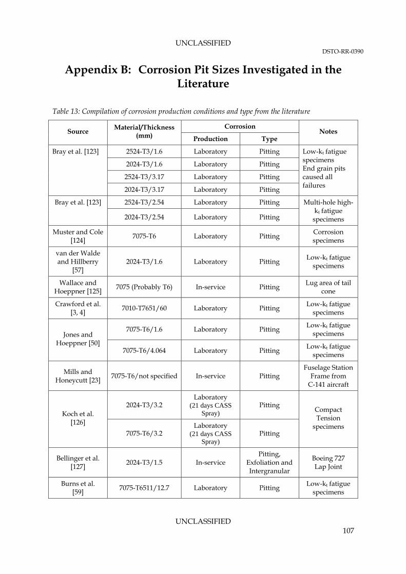
UNCLASSIFIED DSTO-RR-0390
UNCLASSIFIED 107
Appendix B: Corrosion Pit Sizes Investigated in the Literature
Table 13: Compilation of corrosion production conditions and type from the literature
Corrosion Source
Material/Thickness (mm) Production Type
Notes
2524-T3/1.6 Laboratory Pitting
2024-T3/1.6 Laboratory Pitting
2524-T3/3.17 Laboratory Pitting
Bray et al. [123]
2024-T3/3.17 Laboratory Pitting
Low-kt fatigue specimens End grain pits caused all failures
2524-T3/2.54 Laboratory Pitting Bray et al. [123]
2024-T3/2.54 Laboratory Pitting
Multi-hole high-kt fatigue
specimens
Muster and Cole [124]
7075-T6 Laboratory Pitting Corrosion specimens
van der Walde and Hillberry
[57] 2024-T3/1.6 Laboratory Pitting
Low-kt fatigue specimens
Wallace and Hoeppner [125]
7075 (Probably T6) In-service Pitting Lug area of tail
cone
Crawford et al. [3, 4]
7010-T7651/60 Laboratory Pitting Low-kt fatigue
specimens
7075-T6/1.6 Laboratory Pitting Low-kt fatigue
specimens Jones and Hoeppner [50]
7075-T6/4.064 Laboratory Pitting Low-kt fatigue
specimens
Mills and Honeycutt [23]
7075-T6/not specified In-service Pitting Fuselage Station
Frame from C-141 aircraft
2024-T3/3.2 Laboratory
(21 days CASS Spray)
Pitting Koch et al.
[126]
7075-T6/3.2 Laboratory
(21 days CASS Spray)
Pitting
Compact Tension
specimens
Bellinger et al. [127]
2024-T3/1.5 In-service Pitting,
Exfoliation and Intergranular
Boeing 727 Lap Joint
Burns et al. [59]
7075-T6511/12.7 Laboratory Pitting Low-kt fatigue
specimens

UNCLASSIFIED DSTO-RR-0390
UNCLASSIFIED 108
Corrosion Source
Material/Thickness (mm) Production Type
Notes
Cook et al. [21]
7050-T76/4.8 Laboratory Pitting Cold expanded high-kt fatigue
specimens
Codaro et al. [128]
7050-T7451 Laboratory Pitting Corrosion specimens
Gruenberg et al. [54]
2024-T3/1.6
Laboratory (72 hours as per
ASTM G110) [99]
Pitting
Tensile Test Specimens –
low-kt
Harmsworth [129]
2024-T4/not specified Laboratory
(72 hours salt spray)
Pitting
Rotating bending low-kt
fatigue specimens
Burns et al. [60]
7075-T651/50.8
Laboratory (Potentiostatic corrosion or 3 hours EXCO
exposure)
Pitting Low-kt fatigue
specimens
Koul [130]
7075-T6/2 Laboratory (Prohesion
spray) Pitting
Low-kt fatigue specimens
Rokhlin et al. [131]
2024-T3/1.6 EDM EDM Low-kt fatigue
specimens
2024-T3/6 EXCO
(0 to 244 h) Pitting &
Exfoliation Fatigue
specimens Sharp et al. [120]
7075-T6/6 EXCO
(0 to 244 h) Pitting &
Exfoliation Fatigue
specimens
Shekhter et al. [52]
Alclad 7075-T6/3
Laboratory (Aerosol NaCl
solution) Pitting
High-kt fatigue specimens
Smith et al. [132]
7075-T6 In-service Pitting Bolthole in
NASA Space Shuttle wheels
7075-T6 EDM EDM Low-kt fatigue
specimen
Wei [133]
2024-T3/Thickness not stated
500 h in 0.5M NaCl solution
Pitting Multiple
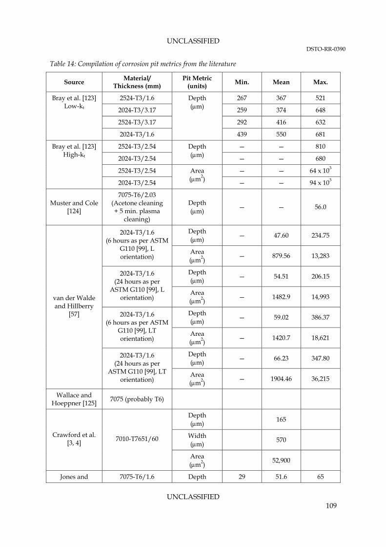
UNCLASSIFIED DSTO-RR-0390
UNCLASSIFIED 109
Table 14: Compilation of corrosion pit metrics from the literature
Source Material/ Thickness (mm)
Pit Metric (units)
Min. Mean Max.
2524-T3/1.6 267 367 521
2024-T3/3.17 259 374 648
2524-T3/3.17 292 416 632
Bray et al. [123] Low-kt
2024-T3/1.6
Depth (m)
439 550 681
2524-T3/2.54 — — 810
2024-T3/2.54
Depth (m) — — 680
2524-T3/2.54 — — 64 x 103
Bray et al. [123] High-kt
2024-T3/2.54
Area (m2) — — 94 x 103
Muster and Cole [124]
7075-T6/2.03 (Acetone cleaning + 5 min. plasma
cleaning)
Depth (m)
— — 56.0
Depth (m)
— 47.60 234.75 2024-T3/1.6 (6 hours as per ASTM
G110 [99], L orientation)
Area (m2)
— 879.56 13,283
Depth (m)
— 54.51 206.15 2024-T3/1.6 (24 hours as per
ASTM G110 [99], L orientation)
Area (m2)
— 1482.9 14,993
Depth (m)
— 59.02 386.37 2024-T3/1.6 (6 hours as per ASTM
G110 [99], LT orientation)
Area (m2)
— 1420.7 18,621
Depth (m)
— 66.23 347.80
van der Walde and Hillberry
[57]
2024-T3/1.6 (24 hours as per
ASTM G110 [99], LT orientation)
Area (m2)
— 1904.46 36,215
Wallace and Hoeppner [125]
7075 (probably T6)
Depth (m)
165
Width (m)
570 Crawford et al.
[3, 4] 7010-T7651/60
Area (m2)
52,900
Jones and 7075-T6/1.6 Depth 29 51.6 65

UNCLASSIFIED DSTO-RR-0390
UNCLASSIFIED 110
Source Material/ Thickness (mm)
Pit Metric (units)
Min. Mean Max.
Hoeppner [50] 7075-T6/4.064 (m) 42 58.4 75
Mills and Honeycutt [23]
7075-T6/not specified
Depth (m)
— — 200
Depth (m)
~0.2 ~3 ~10 2024-T3/3.2 (CASS Spray) Area
(m2) ~300 ~10,000 ~106
Depth (m)
~10 ~100 ~1,000
Koch et al. [126]
7075-T6/3.2 (CASS Spray) Area
(m2) ~300 ~10,000 ~106
Bellinger et al. [127]
2024-T3 Depth (m)
— 48 144
Burns et al. [59]
7075-T6511/12.7 Depth (m)
— ~330 ~480
Depth (m)
3 — 8 7050-T76/4.8 (1 hr
exposure 3.5% NaCl) Area (m2)
110 — 210
Depth (m)
7 — 25
Cook et al. [21]
7050-T76/4.8 (24 hr exposure 3.5% NaCl) Area
(m2) 110 — 9,100
Depth (m)
2 4 13
Width (m)
1 9 54 Codaro et al.
[128]
7050-T7451 (2 day
salt spray) Area (m2)
5 60 410
Depth (m)
— 9 36
Width (m)
— 19 160 7075-T6/2
(1 day salt fog as per ASTM G-85)
Length (m)
— 36 240
Depth (m)
— 12 35
Sankaran et al [134]
7075-T6/2 (2 days salt fog as per
ASTM G-85) Width (m)
— 61 200
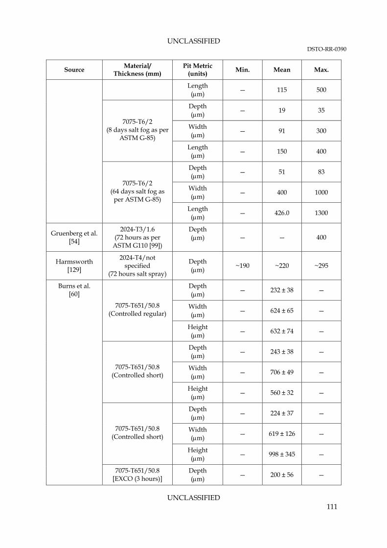
UNCLASSIFIED DSTO-RR-0390
UNCLASSIFIED 111
Source Material/ Thickness (mm)
Pit Metric (units)
Min. Mean Max.
Length (m)
— 115 500
Depth (m)
— 19 35
Width (m)
— 91 300 7075-T6/2
(8 days salt fog as per ASTM G-85)
Length (m)
— 150 400
Depth (m)
— 51 83
Width (m)
— 400 1000 7075-T6/2
(64 days salt fog as per ASTM G-85)
Length (m)
— 426.0 1300
Gruenberg et al. [54]
2024-T3/1.6 (72 hours as per
ASTM G110 [99])
Depth (m) — — 400
Harmsworth [129]
2024-T4/not specified
(72 hours salt spray)
Depth (m)
~190 ~220 ~295
Depth (m)
— 232 ± 38 —
Width (m)
— 624 ± 65 — 7075-T651/50.8
(Controlled regular)
Height (m)
— 632 ± 74 —
Depth (m)
— 243 ± 38 —
Width (m)
— 706 ± 49 — 7075-T651/50.8
(Controlled short)
Height (m)
— 560 ± 32 —
Depth (m)
— 224 ± 37 —
Width (m)
— 619 ± 126 — 7075-T651/50.8
(Controlled short)
Height (m)
— 998 ± 345 —
Burns et al. [60]
7075-T651/50.8 [EXCO (3 hours)]
Depth (m)
— 200 ± 56 —

UNCLASSIFIED DSTO-RR-0390
UNCLASSIFIED 112
Source Material/ Thickness (mm)
Pit Metric (units)
Min. Mean Max.
Width (m)
— 900 ± 239 —
Height (m)
— — —
Depth (m)
— 10 50 Koul [130]
7075-T6/2 (~1600 hours
Prohesion spray) Surface Area (m2)
— 1x10⁴ 1x10⁶
Depth (m)
170 175 185 Rokhlin et al.
[131] 2024-T3/1.6
Diameter (m)
230 240 250
2024-T3/6 Depth (m)
60 — 100 Sharp et al.
[120] 7075-T6/6
Depth (m)
— — 100
Shekhter et al. [52]
Alclad 7075-T6/3
Depth (m)
7 35 70
Smith et al. [132]
7050 no temper stated (Shuttle wheel)
Depth (m)
— 500 1,000
7050/12.7
no temper stated (Laboratory)
Depth (m)
~250 ~750 ~1,500
Wei [133]
2024-T3 Depth (m)
— — 300
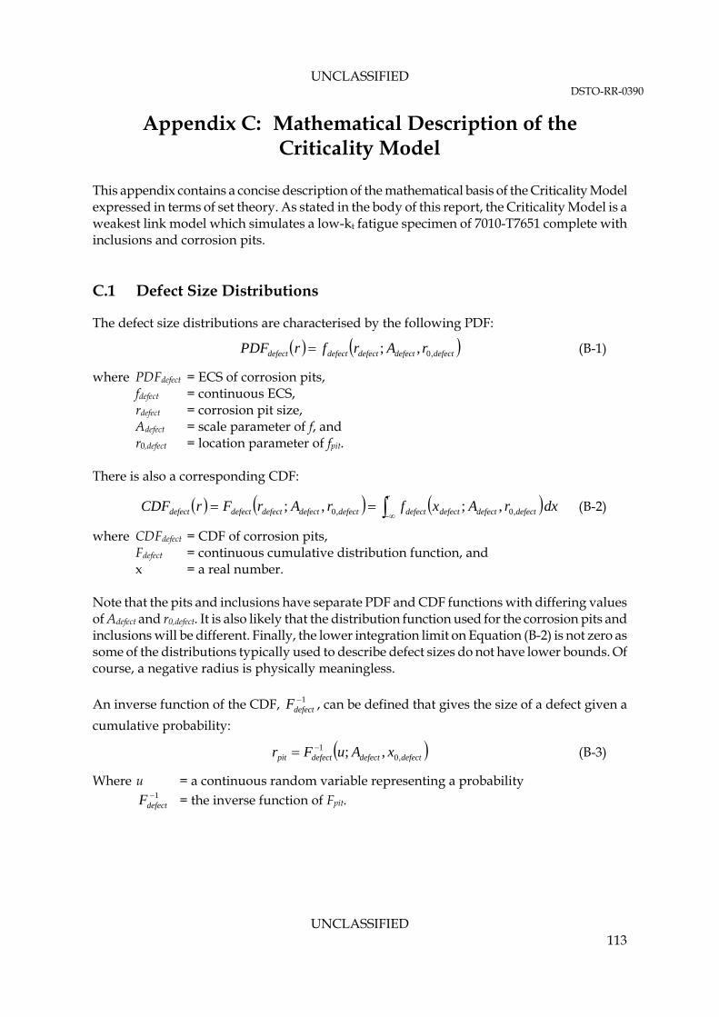
UNCLASSIFIED DSTO-RR-0390
UNCLASSIFIED 113
Appendix C: Mathematical Description of the Criticality Model
This appendix contains a concise description of the mathematical basis of the Criticality Model expressed in terms of set theory. As stated in the body of this report, the Criticality Model is a weakest link model which simulates a low-kt fatigue specimen of 7010-T7651 complete with inclusions and corrosion pits. C.1 Defect Size Distributions
The defect size distributions are characterised by the following PDF:
defectdefectdefectdefectdefect rArfrPDF ,0,; (B-1)
where PDFdefect = ECS of corrosion pits, fdefect = continuous ECS, rdefect = corrosion pit size, Adefect = scale parameter of f, and r0,defect = location parameter of fpit. There is also a corresponding CDF:
r
defectdefectdefectdefectdefectdefectdefectdefectdefect dxrAxfrArFrCDF ,0,0 ,;,; (B-2)
where CDFdefect = CDF of corrosion pits, Fdefect = continuous cumulative distribution function, and x = a real number. Note that the pits and inclusions have separate PDF and CDF functions with differing values of Adefect and r0,defect. It is also likely that the distribution function used for the corrosion pits and inclusions will be different. Finally, the lower integration limit on Equation (B-2) is not zero as some of the distributions typically used to describe defect sizes do not have lower bounds. Of course, a negative radius is physically meaningless. An inverse function of the CDF, 1
defectF , can be defined that gives the size of a defect given a
cumulative probability:
defectdefectdefectpit xAuFr ,01 ,; (B-3)
Where u = a continuous random variable representing a probability 1
defectF = the inverse function of Fpit.
UNCLASSIFIED DSTO-RR-0390
UNCLASSIFIED 114
C.2 Defect Location Description
The location of a given defect on the model coupon can be described by its location along the centreline of the specimen. This location was described as a distance, di, from the midpoint of the specimen. The value of di in millimetres was uniformly distributed in the range:
2
982
98 corrosioni
corrosion ld
l (B-4)
where lcorrosion = the length of the corrosion strike C.3 Fatigue Crack Growth Driving Force
The crack driving force at a defect is given by:
bwRafK RN ,,;,max (B-5)
Where fN-R = the Newman and Raju K-solution for a semi-elliptical surface crack [66], a = crack length, max = the maximum local stress experienced by the defect,
R = the load ratio =max
min
,
min = the minimum local stress experienced by the defect, and w, b = the specimen width and thickness. C.4 Fatigue Life Estimation
The fatigue life of a crack initiating from a given defect is:
bwRKfN THf ,,; (B-6)
Where fH-T is a Harter-T piecewise integral of the Walker equation which is:
nmRKCdN
da 11 (B-7)
Where m = Walker exponent, n = Paris law exponent, and C = Paris Law coefficient This, upon integration becomes:
daKRC
Nf
i
a
a
nm 11
1 (B-8)
The Walker exponent, m, in the above equation is used to model the effect of R on fatigue crack growth rates. It has no other physical significance. Using the Harter-T method K, m
UNCLASSIFIED DSTO-RR-0390
UNCLASSIFIED 115
and n are all functions of a. As such equation (B-8) cannot be solved analytically and must be solved numerically. This is the function of AFGROW in the current work43. The model described here is a weakest link model. It models the growth of fatigue cracks from a number of initiating defects on the surface of the component. Failure occurs and is complete when a single one of these defects fails. That is, the component’s fatigue life is:
Τflfifffcomponentf NNNNNN min,,,,,min ,,2,1,, (B-9)
Where: denotes a set, T = the set of all defects Nf,i = the fatigue life of the i-th defect, and l = the total number of corrosion pit and inclusion defects. In the above equation a component that does not fail due to fatigue is assigned a fatigue life of infinity (∞)44. There are two sets of defects, corrosion pits and inclusions, on the component. Each of these defects sets has a corresponding set of fatigue lives from which a minimum fatigue life for that kind of defect can be obtained, i.e.:
Corrosion pits: Cfjfifffpitsminf NNNNNN min,,,,,min ,,2,1,,, (B-10)
Where j = the number of corrosion pits, and C = the set of all corrosion pits. and
Particle: Pfkfiffficlesf,min,part NNNNNN min,,,,,min ,,2,1, (B-11)
Where k = number of inclusions, and P = the set of all inclusions. Note that kjl and PCT The fatigue life of the component as a whole regardless of critical defect type is:
f,min,piticlef,min,partcomponentf NNN ,min, (B-12)
This equation is equivalent to equation (B-9). C.5 Limit State Equation
It is possible to formulate a limit state equation G from the above:
f,min,piticlef,min,part NNG (B-13)
43 Note that any fatigue crack growth prediction code could be used here. DeBartolo for example used FASTRAN [53, 90, 91]. 44 Igor Pro allows the use of the symbols ‘INF’ to represent infinity and ‘-INF’ to represent negative infinity. INF is defined as being greater than (by definition) any other real or integer number.

UNCLASSIFIED DSTO-RR-0390
UNCLASSIFIED 116
where G < 0: UNSAFE: unexpected failure from a fatigue crack initiated at a corrosion pit G = 0: LIMIT STATE: Nf,min,particle = Nf,min,pit G > 0: SAFE: expected failure from a fatigue crack initiated at an inclusion
12
10
8
6
4
2
0
Pro
babi
lity
Den
sity
x 1
0-6
900x103800700600500400
Fatigue Cycles
Corrosion Pits Inclusions
Figure 74: Plot of the PDFs of the predicted fatigue life distributions for corrosion pits and inclusions.
The probability of fracture due to a corrosion pit is equal to the probability that G < 0. That is:
0CDF
sgn12
1
0PrPr
1
G
Gp
GFractureCorrosionp
ii (B-14)
where Gi = the limit function of the i-th iteration p = the number of replicates, and
sgn(x) =
01
01
x
x
The value of the CDF of G at G = 0 is the probability that failure is due to corrosion.
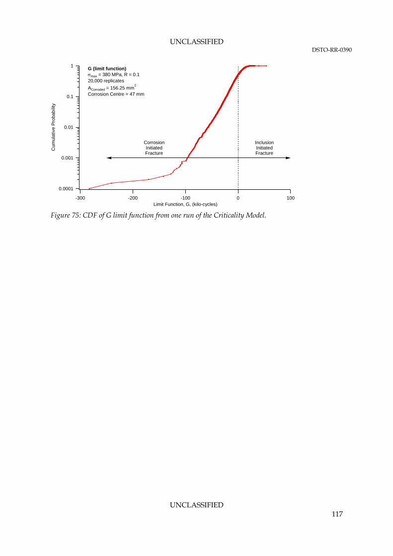
UNCLASSIFIED DSTO-RR-0390
UNCLASSIFIED 117
0.0001
0.001
0.01
0.1
1
Cum
ulat
ive
Pro
babi
lity
-300 -200 -100 0 100Limit Function, G, (kilo-cycles)
G (limit function) max = 380 MPa, R = 0.1 20,000 replicates
ACorroded = 156.25 mm2
Corrosion Centre = 47 mm
CorrosionInitiatedFracture
InclusionInitiatedFracture
Figure 75: CDF of G limit function from one run of the Criticality Model.

UNCLASSIFIED DSTO-RR-0390
UNCLASSIFIED 118
Appendix D: Source Code for Criticality Model
The source code for the Criticality Model described in this report is available to approved persons on request. The source code can be obtained by emailing [email protected]

UNCLASSIFIED DSTO-RR-0390
UNCLASSIFIED 119
Appendix E: Marker Band Fatigue Crack Growth Dataset
Table 15: Marker Band fatigue crack growth dataset
Load Ratio Fatigue Crack Growth Rate
(m/cycle) -0.3 0.1 0.5
1x10-15 0.0185 0.0194 0.0168
5x10-15 0.0321 0.0337 0.0293
1x10-14 0.0408 0.0428 0.0372
5x10-14 0.0711 0.0745 0.0647
1x10-13 0.0902 0.0946 0.0822
5x10-13 0.1571 0.164 0.143
1x10-12 0.199 0.209 0.181
5x10-12 0.347 0.364 0.316
1x10-11 0.44 0.462 0.401
5x10-11 0.766 0.804 0.698
1x10⁻¹⁰ 0.973 1.02 0.886
5x10⁻¹⁰ 1.69 1.77 1.54
1x10⁻⁹ 2.15 2.25 1.95
5x10⁻⁹ 3.74 3.92 3.4
1x10⁻⁸ 4.75 4.98 4.32
5x10⁻⁸ 8.26 8.66 7.53
1x10⁻⁷ 10.4 11 9.55
5x10⁻⁷ 18.2 19.1 16.6
1x10⁻⁶ 23.1 24.3 21.1
5x10⁻⁶ 40.3 42.3 36.7
1x10⁻⁵ 51.2 53.7 46.6
5x10⁻⁵ 89.1 93.4 81.1
1x10⁻⁴ 113 118 103
5x10⁻⁴ 196 206 179
1x10⁻³ 249 262 227

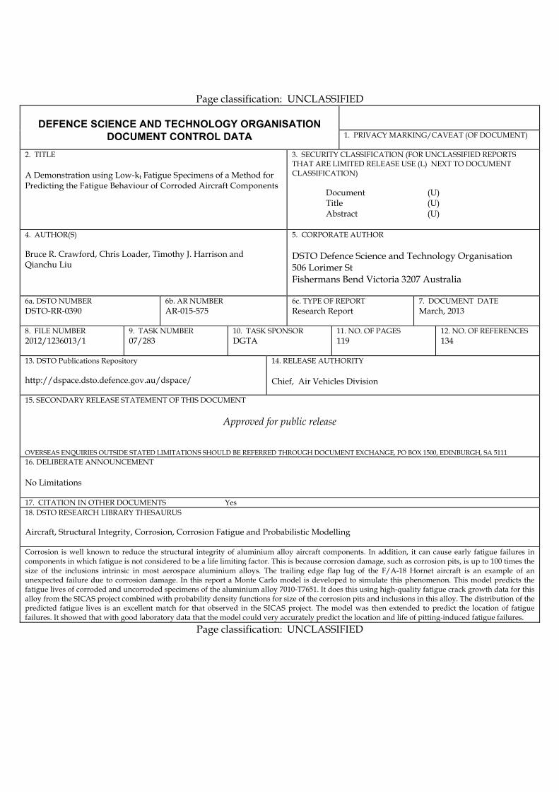
Page classification: UNCLASSIFIED
DEFENCE SCIENCE AND TECHNOLOGY ORGANISATION
DOCUMENT CONTROL DATA 1. PRIVACY MARKING/CAVEAT (OF DOCUMENT)
2. TITLE A Demonstration using Low-kt Fatigue Specimens of a Method for Predicting the Fatigue Behaviour of Corroded Aircraft Components
3. SECURITY CLASSIFICATION (FOR UNCLASSIFIED REPORTS THAT ARE LIMITED RELEASE USE (L) NEXT TO DOCUMENT CLASSIFICATION) Document (U) Title (U) Abstract (U)
4. AUTHOR(S) Bruce R. Crawford, Chris Loader, Timothy J. Harrison and Qianchu Liu
5. CORPORATE AUTHOR DSTO Defence Science and Technology Organisation 506 Lorimer St Fishermans Bend Victoria 3207 Australia
6a. DSTO NUMBER DSTO-RR-0390
6b. AR NUMBER AR-015-575
6c. TYPE OF REPORT Research Report
7. DOCUMENT DATE March, 2013
8. FILE NUMBER 2012/1236013/1
9. TASK NUMBER 07/283
10. TASK SPONSOR DGTA
11. NO. OF PAGES 119
12. NO. OF REFERENCES 134
13. DSTO Publications Repository http://dspace.dsto.defence.gov.au/dspace/
14. RELEASE AUTHORITY Chief, Air Vehicles Division
15. SECONDARY RELEASE STATEMENT OF THIS DOCUMENT
Approved for public release OVERSEAS ENQUIRIES OUTSIDE STATED LIMITATIONS SHOULD BE REFERRED THROUGH DOCUMENT EXCHANGE, PO BOX 1500, EDINBURGH, SA 5111 16. DELIBERATE ANNOUNCEMENT No Limitations 17. CITATION IN OTHER DOCUMENTS Yes 18. DSTO RESEARCH LIBRARY THESAURUS Aircraft, Structural Integrity, Corrosion, Corrosion Fatigue and Probabilistic Modelling Corrosion is well known to reduce the structural integrity of aluminium alloy aircraft components. In addition, it can cause early fatigue failures in components in which fatigue is not considered to be a life limiting factor. This is because corrosion damage, such as corrosion pits, is up to 100 times the size of the inclusions intrinsic in most aerospace aluminium alloys. The trailing edge flap lug of the F/A-18 Hornet aircraft is an example of an unexpected failure due to corrosion damage. In this report a Monte Carlo model is developed to simulate this phenomenon. This model predicts the fatigue lives of corroded and uncorroded specimens of the aluminium alloy 7010-T7651. It does this using high-quality fatigue crack growth data for this alloy from the SICAS project combined with probability density functions for size of the corrosion pits and inclusions in this alloy. The distribution of the predicted fatigue lives is an excellent match for that observed in the SICAS project. The model was then extended to predict the location of fatigue failures. It showed that with good laboratory data that the model could very accurately predict the location and life of pitting-induced fatigue failures.
Page classification: UNCLASSIFIED