A Delay Estimation Technique for Single and

Double-track Railroads

Pavankumar Murali∗, Maged M. Dessouky, Fernando Ordonez,

and Kurt Palmer

{pmurali, maged, fordon, kpalmer}@usc.edu

Dept. of Industrial & Systems Engineering, University of Southern California,

3715 McClintock Ave., GER 240, Los Angeles, CA 90089-0193, USA

February 8, 2009

Abstract

To route and schedule trains over a large complex network can be computationally

intensive. One way to reduce complexity could be to “aggregate” suitable sections of

a network. In this paper, we present a simulation-based technique to generate delay

estimates over track segments as a function of traffic conditions, as well as network

topology. We test our technique by comparing the delay estimates obtained for a

network in Los Angeles with the delays obtained from the simulation model developed

by Lu et al. (2004), which has been shown to be representative of the real-world delay

values. Railway dispatchers could route and schedule freight trains over large networks

by using our technique to estimate delay across aggregated network sections.

∗Corresponding author

1

1 Introduction

In the United States, railways offer a cost-effective means to trans-continentally move goods

from ports to various inland destinations. However, mergers and abandonment of rail lines,

and booming international trade have contributed to the existing congestion in rail network

systems in the Los Angeles area, and other similar regions in the United States. Similarly,

in the eastern US, the CSX and NS railroads are attempting to cope with traffic levels much

higher than what they were designed to handle.

There is clearly a need among US freight railroads for better analytical tools to manage their

capacity and scheduling. A challenging problem in this context is to determine the effect of

additional trains on a railroad. This problem requires estimating the travel times and delays

in the network, and assigning trains to routes based on the expected running times in order

to balance the railroad traffic, and to reject or defer the train(s) that would overload the

network and result in unacceptable delays in traveling through the network. In the United

States and in Europe, passenger trains have utmost priority and follow timetables. Freight

trains have a lower priority, and are sent on routes and scheduled to minimize their impact on

passenger trains. There is considerable variability associated with train departures from their

stations due to uncertainty in loading time and crew handling. However, the variabilities

are more pronounced in the case of freight trains.

Various kinds of estimation techniques can be used to study how the delay varies with a

change in the traffic conditions and/or the railway network topology. The difference between

the actual running time and the free running time is termed as travel time delay or, simply,

delay. The free running time of a train over a network is defined as the time the train takes to

traverse the network, when traveling at its maximum allowable speed and not experiencing

delays due to other train(s). The actual running time is the time a train travels to reach its

destination when there are other trains in the network. For freight trains, delays can be of

two types, namely, direct and knock-on (or indirect) delays. Direct delays to trains are a

consequence of minor delays at a station. These are not as a result of other trains traveling

along the same lines. Knock-on delays are those which are induced into the system due to

a direct and/or knock-on delay to another train in the network. It is transferred from one

2

train to, possibly, all the other trains in the vicinity.

The capacity of a railway network and the delay across it are closely related. The delays

encountered by trains under different operating assumptions can be used to evaluate the

capacity of a section of a network, which is referred to as a subnetwork. Capacity can

be defined as the maximum number of trains that can traverse a network, or a section of a

network, without resulting in a deadlock. Burdett and Kozan (2006) define absolute capacity

as the theoretical capacity value that is realized only when critical sections of a network are

saturated. On the other hand, actual capacity is the number of trains that can safely coexist

in a network, or a portion of it, when interference delays are taken into consideration. Both

measures of capacity are measured over time. Absolute capacity can be used as an upper

bound for planning purposes.

The actual capacity of any section of a railway network cannot be a unique value, and it

is neither easily defined nor quantified. It depends on the average minimum headway time

between consecutive trains, the signalling system, train speeds, trackage configuration etc.

For instance, single-tracks with sidings can accommodate more trains and enable crossings

and overtakes than those without. Signals can increase capacity by reducing the required

headway between trains. Delay estimation and capacity analysis in railway transportation is

dependent on various operational aspects. The first aspect is the trackage configuration. The

network can consist of single, double, triple or even more track. Single tracks are common in

the case of North America while double and triple tracks are common in Europe. Normally,

the level of complexity in urban areas is higher than in rural areas because they contain

many junctions. A train can block the movement of other trains when it tries to cross over

at a junction from one line to another. The second aspect is the variation in speed limits

on different track segments and junctions. Furthermore, passenger trains and freight trains

can have different maximum speeds even though their paths may use the same tracks, but

not necessarily at the same time. If a train passes a junction by changing lines, the speed

limit at the junction will be enforced. While single speed limits are common on networks

in rural areas, multiple speed limits are common in metropolitan areas. A lower speed-limit

over a subnetwork tends to increase travel time delays. The third aspect is the characteristic

of each train in the rail network such as priority, train length, speed, acceleration rate and

3

deceleration rate. Generally, passenger trains have higher priority than freight trains. If

two trains want to seize the same track simultaneously, the train with the lower priority

should wait and stop until the train with higher priority passes. Sometimes trains cannot

be dispatched at their maximum speed because of the track speed limit. Acceleration and

deceleration rates need to be considered in order to increase or reduce speed without violating

the speed limit. This results in a nonlinear function to represent the movement of trains.

In this paper, we present a delay estimation technique that models delay as a function of

the train mix and the network topology. These delay estimates can be used to route and

schedule trains over a large complex network. One way to reduce the complexity of routing

and scheduling could be to “aggregate” suitable sections of a network in our analysis. An

estimate of the expected travel time delay with traffic in the aggregated section would need

to be fed to a routing and scheduling model so that trains can estimate, well in advance,

the delay they would experience along each possible route to their destination. The delay

estimation technique discussed in this paper reflects on how the delay in the aggregated

section of the network varies with each additional train. Once a delay estimation equation

has been generated by our technique, it can be used to estimate delay and capacity of a

network section with physical attributes within the range of those of the generic networks

used in the experiments. That is, individual simulations need not be run for every aggregated

network section.

This paper is organized as follows. In Section 2, we give a brief insight into the prior work

done in developing delay models for railways. In Section 3, we describe our methodology in

estimating travel time delays in a subnetwork containing double-tracks or single-tracks. We

validate our models by using them to predict delays on test networks, as well as rail networks

in the Los Angeles area, and comparing it with the generated delays from a simulation model.

2 Previous work

In order to minimize delays in delivering freight goods, each train has to travel on a route

that minimizes travel time, meet/pass interferences and expected delays. To accomplish

4

this, it is imperative to have a robust delay estimation technique that is capable of accu-

rately predicting travel time delay as a function of the operating parameters. There exists

a considerable amount of rail transport literature that aims to better comprehend the na-

ture of knock-on delays. In the past, researchers have used either analytical methods or

simulation-based methods to study delay and/or capacity assessment in railroads.

2.1 Analytical Models

One of the earliest analytical models on capacity and delay assessment was developed by

Frank (1966). He studied delay on a single track with unidirectional and bidirectional traffic.

By restricting only one train on each link between sidings and using single train speeds

and deterministic travel times, he estimated the number of trains that could travel on the

network. Petersen (1974) extended this work to accommodate for two different train speeds.

He assumed independent and uniformly distributed departure times, equally spaced sidings

and a constant delay for each encounter between two trains. Chen et al. (1990) extended

Petersen’s model to present a technique to calculate delay for different types of trains over a

specified single track section as a function of the schedules of the trains and the dispatching

policies. They assumed sidings to be equally distributed, that faster trains can overtake

slower trains, meets and overtakes occur only between 2 trains at a time, and there exists a

fixed probability Pi,j of a train i getting delayed by a train j. This modeling technique was

extended by Parker et al. (1990) to a partially double-track rail network which consisted of

a single-track section with sidings and double-track sections. Similar to the previous work,

trains depart according to their scheduled departure times. The train to be delayed during a

meet (or overtake) is determined by a trade-off between the lateness of the train with respect

to its schedule and the overall priority of the train. Carey et al. (1994) studied the effects

of knock-on delays between two trains on a single-track. They used non-linear regression to

develop stochastic approximations of the relation between scheduled headways and knock-on

delays, and tested these approximations by conducting detailed stochastic simulation of the

interactions between trains as they traverse sections of the network. Ozekici et al. (1994)

used Markov chain techniques to study the effects of various dispatching patterns and arrival

5

patterns of passengers on knock-on delays and passenger waiting times. Given a travel time

probability density function for a train on a track link, a departure time transition matrix

was constructed for the calculation of the expected departure delay. Higgins et al. (1998)

presented an analytical model to quantify the positive delay for individual passenger trains,

track links and schedule as a whole in an urban rail network. The network they considered

has multiple unidirectional and bidirectional tracks, crossings and sidings. Yuan (2006, 2008)

proposed probability models that provide a realistic estimate of knock-on delays and the use

of track capacity. The proposed model reflects speed fluctuation due to signals, dependencies

of dwell times at stations and stochastic interdependencies due to train movements. D’Ariano

(2008) studied delay propagation by decomposing a long time horizon into tractable intervals

to be solved in cascade, and using advanced Conflict Detection and Resolution with Fixed

Routes (CDRFR) algorithms. These algorithms are used to detect and globally solve train

conflicts on each time interval.

Queuing theory is another methodology that has been used for estimating delay in railroads.

Greenberg et al. (1988) presented queuing models for predicting dispatching delays on a low

speed, single track rail network supplemented with sidings and/or alternate routes. Train

departures are modeled as a Poisson process, and the slow transit speed and deterministic

travel times enable them to travel with close headways. This work assumes sidings to have

infinite capacity. Huisman et al. (2001) investigated delays to a fast train caught behind

slower ones by capturing both scheduled and unscheduled movements. This is modeled as an

infinite server G/G/∞ re-sequencing queue, where the running time distributions for each

train service are obtained by solving a system of linear differential equations. Wendler (2007)

presented an approach for predicting waiting times using a M/SM/1/∞ queuing system with

a semi-Markovian kernel. The arrival process is determined by the requested train paths.

The description of the service process is based on an application of the theory of blocking

times and minimum headway times.

A bottleneck approach is one way to determine the absolute capacity of a network, by identi-

fying the maximum number of trains that can travel through the track segments constituting

a bottleneck in a given time period. De Kort et al. (2003) considered the problem of de-

termining the capacity of a planned railway infrastructure layout under uncertainties for

6

an unknown demand of service. The capacity assessment problem for this generic model

is translated into an optimization problem. Burdett and Kozan (2006) developed capacity

analysis techniques and methodologies for estimating the absolute (theoretical) traffic car-

rying ability of facilities over a wide range of defined operational conditions. Specifically,

they address the factors on which the capacity of a network depends on, namely, propor-

tional mix of trains, direction of travel, length of trains, planned dwell times of trains, the

presence of crossing loops and intermediate signals in corridors and networks. Gibson et al.

(2002) also developed a regression model to define a correlation between capacity utilization

and reactionary delay. Landex et al. (2006) and Kaas (1998) discussed techniques to cal-

culate capacity utilization for railway lines with single and multiple tracks, as per the UIC

(International Union of Railways) 406 method.

2.2 Simulation Models

Simulation techniques can be used to study direct, knock-on and compound delays and ripple

effects from conflicts at complex junctions, terminals, railroad crossings, network topology,

train and traffic parameters. The compound interaction effects of these factors cannot be

effectively captured in an analytical delay estimation model. Petersen et al. (1982) present

a structured model for rail line simulation. They divide the rail line into track segments

representing the stretches of track between adjacent switches and develop algebraic rela-

tionships to represent the model logic. Dessouky et al. (1995) use a simulation modeling

methodology to analyze the capacity of tracks and delay to trains in a complex rail network.

Their methodology considers both single and double-track lines and is insensitive to the size

of the rail network. Their model has a distinctive advantage of accounting for track speed-

limits, headways, and actual train lengths, speed-limits acceleration and deceleration rates

in order to determine the track configuration that minimizes congestion delay to trains. This

work is extended by Lu et al. (2004). Hallowell et al. (1998) improve upon the work by

Parker et al. (1990) by incorporating dynamic meet/pass priorities in order to approximate

an optimal meet/pass planning process. Extensive Monte Carlo simulations are conducted

to examine the application of an analytical line model for adjusting real-world schedules to

7

improve on-time performance and reduce delay. Krueger (1999) uses simulation to develop

a regression model to define the relationship between train delay and traffic volume. The

parameters involved are network parameters, traffic parameters and operating parameters.

A majority of the prior work on delay estimation and capacity assessment for railway net-

works does not explicitly consider the vital and complex interactions between traffic, oper-

ating and network parameters. In the case of the analytical models, heavy assumptions are

made in order to maintain the complexity of the problem within solvable bounds, thereby

rendering the problem to be far off from real-life rail operations. Furthermore, these models

may be incapable of recognizing the dynamic nature of capacity and knock-on delays in-

volving more than two trains. More often than not, delay or capacity estimation is unlikely

to be the final step in railway operations planning. Instead, a dispatcher might use these

estimated values in railway routing and scheduling, that is, to route a set of trains over

tracks with the minimum expected delay so as to minimize the overall system delay. For

such purposes, it would be beneficial to design simple delay estimation models that could

be easily integrated with or incorporated into a routing, scheduling or dispatching model.

Analytical models requiring algorithms to solve a system of equations might not be the best

option for this purpose. Simulation models, on the other hand, would enable us to develop

simple, yet accurate, algebraic relationships that better capture the stochastic nature of the

interactions between the traffic, operating and network parameters, and their impact on

travel time delays.

In this paper, we use simulation techniques to develop accurate and simple regression-based

delay estimation models that can then be used with railway routing and scheduling models.

3 A Delay Estimation Methodology

In this section, we present a delay estimation methodology, based on Design of Experiments

techniques, that can be used to predict delays in railway networks, while capturing interac-

tions between the network, traffic and operating parameters. As explained in detail below,

generic networks are first constructed to represent the range of the physical attributes of the

8

actual networks for which delays are to be estimated. Next, we run simulations representing

train movements through these generic networks, and record the relevant system state data.

Finally, a regression analysis is made to run on the collected data. This regression equation is

shown to accurately estimate the travel time delay on an actual network that has its physical

attributes within the extreme limits of the networks used in the experiments.

To this end, we use the simulation model developed by Lu et al. (2004), which divides the

rail network into track segments. This model considers multiple trackage configurations in

the same rail network with multiple speed limits while accounting for the acceleration and

deceleration limits of the trains. In addition, the freight trains are assumed to arrive at origin

stations following a stochastic arrival process. A central dispatching algorithm decides the

movement of each train in the network considering whether to continue moving at the same

speed, to accelerate or decelerate, or to stop. The algorithm also determines the next track

to be seized from among the multiple alternative tracks. The authors prove this algorithm

to be deadlock-free, while attempting to keep the train delays to a minimum. The modeling

methodology does not depend on the size of the network and is insensitive to the trackage

configuration. Thus, changes to the trackage configuration require changes only to the input

data files. Considering the Downtown Los Angeles - Inland Empire Trade Corridor as an

example, the authors show that the delays experienced by the trains as per the simulation

model are very close to the real-world travel time delays.

This simulation model is used to study the impact of the network topology and traffic

parameters on the delay experienced by trains in traversing a subnetwork. We assume trains

can accelerate and decelerate instantaneously to obey track speed limits, and the simulation

model is modified accordingly. Hence, the maximum speed of a train at each instant of time

is simply set to the constraining speed-limit of the track segment. Furthermore, a Poisson

arrival process is assumed for each train. The control parameters for each simulation are as

follows:

1. λi: the arrival rate of each type of train.

2. L: the length of the subnetwork, that is, the distance in miles between the start and

the end of the subnetwork.

9

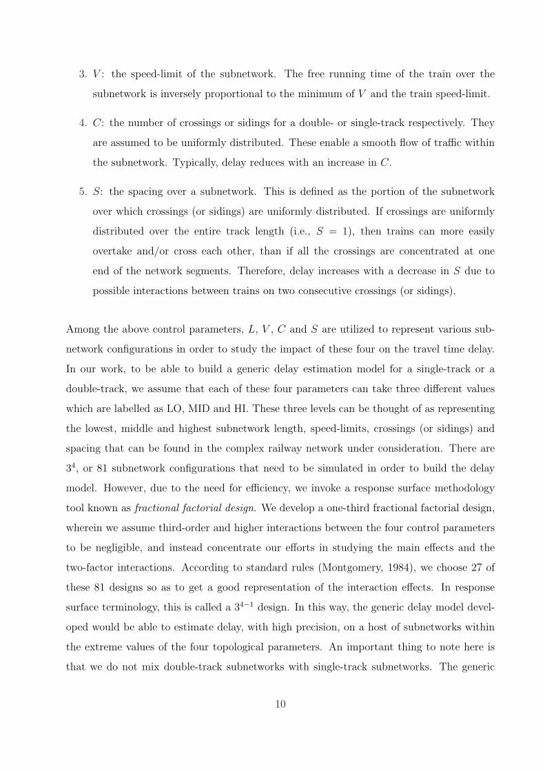
3. V : the speed-limit of the subnetwork. The free running time of the train over the

subnetwork is inversely proportional to the minimum of V and the train speed-limit.

4. C: the number of crossings or sidings for a double- or single-track respectively. They

are assumed to be uniformly distributed. These enable a smooth flow of traffic within

the subnetwork. Typically, delay reduces with an increase in C.

5. S: the spacing over a subnetwork. This is defined as the portion of the subnetwork

over which crossings (or sidings) are uniformly distributed. If crossings are uniformly

distributed over the entire track length (i.e., S = 1), then trains can more easily

overtake and/or cross each other, than if all the crossings are concentrated at one

end of the network segments. Therefore, delay increases with a decrease in S due to

possible interactions between trains on two consecutive crossings (or sidings).

Among the above control parameters, L, V , C and S are utilized to represent various sub-

network configurations in order to study the impact of these four on the travel time delay.

In our work, to be able to build a generic delay estimation model for a single-track or a

double-track, we assume that each of these four parameters can take three different values

which are labelled as LO, MID and HI. These three levels can be thought of as representing

the lowest, middle and highest subnetwork length, speed-limits, crossings (or sidings) and

spacing that can be found in the complex railway network under consideration. There are

34, or 81 subnetwork configurations that need to be simulated in order to build the delay

model. However, due to the need for efficiency, we invoke a response surface methodology

tool known as fractional factorial design. We develop a one-third fractional factorial design,

wherein we assume third-order and higher interactions between the four control parameters

to be negligible, and instead concentrate our efforts in studying the main effects and the

two-factor interactions. According to standard rules (Montgomery, 1984), we choose 27 of

these 81 designs so as to get a good representation of the interaction effects. In response

surface terminology, this is called a 34−1 design. In this way, the generic delay model devel-

oped would be able to estimate delay, with high precision, on a host of subnetworks within

the extreme values of the four topological parameters. An important thing to note here is

that we do not mix double-track subnetworks with single-track subnetworks. The generic

10

delay model is developed separately for each of them.

The simulation is run for each of the 27 subnetwork configurations using AweSim! 2.0

(Pritsker and O’Reilly, 1999), by altering the data files. For each subnetwork configuration,

simulations are run for a fixed ratio of the types of trains traveling through the subnetwork,

and various values of λi for each train type. Two stations are assumed to be present at

either end of a subnetwork, and there are an equal number of trains travelling in either

direction. Trains are made to travel between their respective origin and destination stations.

Furthermore, we also assume that there are no stations in between the origin and destination

stations. During each run, the state of the system is recorded at the arrival times of randomly

selected trains at their respective origin station. At each randomly sampled time instant,

the following data is recorded.

1. Xi: the number of trains of type i in the subnetwork.

2. D1: the number of trains that enter the subnetwork from the opposite direction after

the entry and before the exit of the aforementioned randomly selected train.

3. D2: the number of trains already present in the subnetwork when the randomly selected

train enters the subnetwork and traveling in a direction opposite to it.

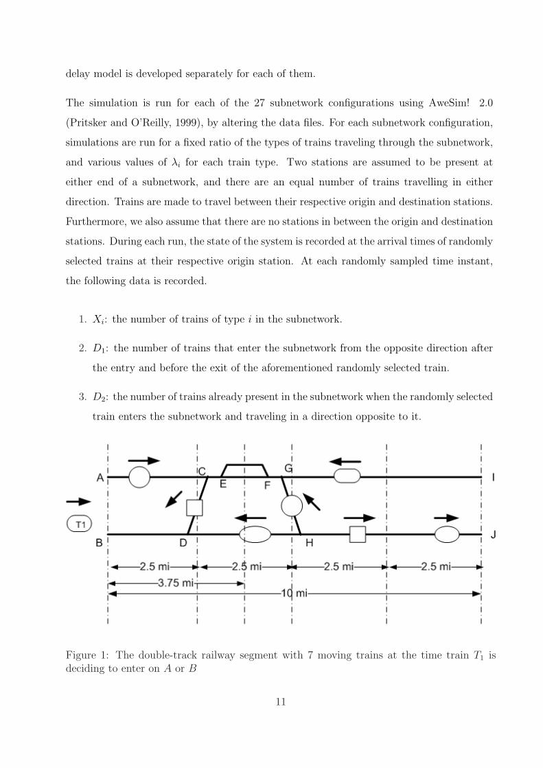
Figure 1: The double-track railway segment with 7 moving trains at the time train T1 isdeciding to enter on A or B

11

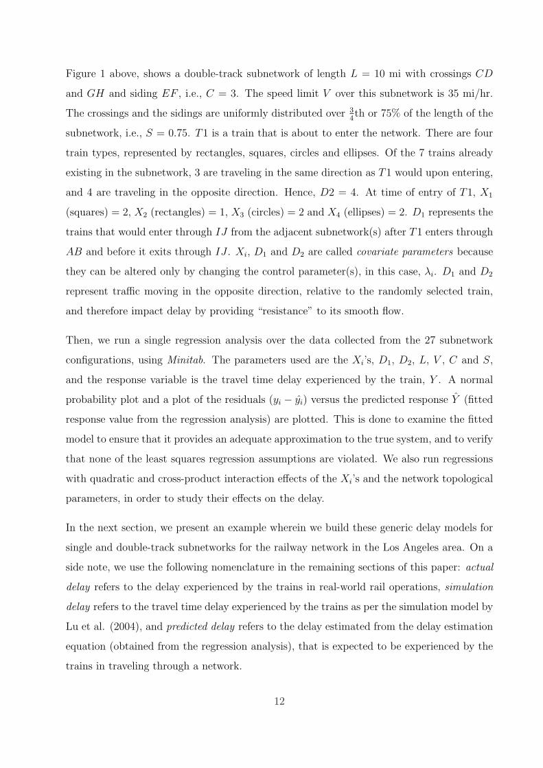
Figure 1 above, shows a double-track subnetwork of length L = 10 mi with crossings CD

and GH and siding EF , i.e., C = 3. The speed limit V over this subnetwork is 35 mi/hr.

The crossings and the sidings are uniformly distributed over 34th or 75% of the length of the

subnetwork, i.e., S = 0.75. T1 is a train that is about to enter the network. There are four

train types, represented by rectangles, squares, circles and ellipses. Of the 7 trains already

existing in the subnetwork, 3 are traveling in the same direction as T1 would upon entering,

and 4 are traveling in the opposite direction. Hence, D2 = 4. At time of entry of T1, X1

(squares) = 2, X2 (rectangles) = 1, X3 (circles) = 2 and X4 (ellipses) = 2. D1 represents the

trains that would enter through IJ from the adjacent subnetwork(s) after T1 enters through

AB and before it exits through IJ . Xi, D1 and D2 are called covariate parameters because

they can be altered only by changing the control parameter(s), in this case, λi. D1 and D2

represent traffic moving in the opposite direction, relative to the randomly selected train,

and therefore impact delay by providing “resistance” to its smooth flow.

Then, we run a single regression analysis over the data collected from the 27 subnetwork

configurations, using Minitab. The parameters used are the Xi’s, D1, D2, L, V , C and S,

and the response variable is the travel time delay experienced by the train, Y . A normal

probability plot and a plot of the residuals (yi − yi) versus the predicted response Y (fitted

response value from the regression analysis) are plotted. This is done to examine the fitted

model to ensure that it provides an adequate approximation to the true system, and to verify

that none of the least squares regression assumptions are violated. We also run regressions

with quadratic and cross-product interaction effects of the Xi’s and the network topological

parameters, in order to study their effects on the delay.

In the next section, we present an example wherein we build these generic delay models for

single and double-track subnetworks for the railway network in the Los Angeles area. On a

side note, we use the following nomenclature in the remaining sections of this paper: actual

delay refers to the delay experienced by the trains in real-world rail operations, simulation

delay refers to the travel time delay experienced by the trains as per the simulation model by

Lu et al. (2004), and predicted delay refers to the delay estimated from the delay estimation

equation (obtained from the regression analysis), that is expected to be experienced by the

trains in traveling through a network.

12

4 Case Study: Los Angeles area Railway Network

The Ports of Los Angeles and Long Beach are the busiest ports on the West Coast. Three

railroad lines, Union Pacific - Alhambra, Union Pacific - San Gabriel and Burlington North-

ern Santa Fe operate service from Los Angeles downtown to the ports. Travel time delays

from the simulation model on this network have been shown by Lu et al. (2004) to be close

to real-world delay values. The trackage in this region is primarily a combination of single

and double-tracks. Crossings and sidings are provided for the purpose of train meets and

overtakes, thereby ensuring a smooth traffic flow. Four types of trains primarily travel on

these tracks - long double stack (8000 feet), intermodal (6000 feet), carload (6500 feet) and

oil (5000 feet). The speed-limits of these trains are 70, 55, 50 and 40 mi/hr respectively.

In our experiments, we assume a fixed ratio of these four train types. For each subnet-

work, multiple simulation runs are performed, each with a different combination of the λi’s.

The primary purpose of this is to get a good representation of the system space, that is,

how the delay varies with different values of Xi, for a fixed setting of the network topology

parameters.

4.1 Delay Estimation for a Double-track Subnetwork

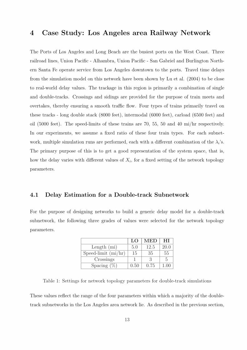
For the purpose of designing networks to build a generic delay model for a double-track

subnetwork, the following three grades of values were selected for the network topology

parameters.

LO MED HILength (mi) 5.0 12.5 20.0

Speed-limit (mi/hr) 15 35 55Crossings 1 3 5

Spacing (%) 0.50 0.75 1.00

Table 1: Settings for network topology parameters for double-track simulations

These values reflect the range of the four parameters within which a majority of the double-

track subnetworks in the Los Angeles area network lie. As described in the previous section,

13

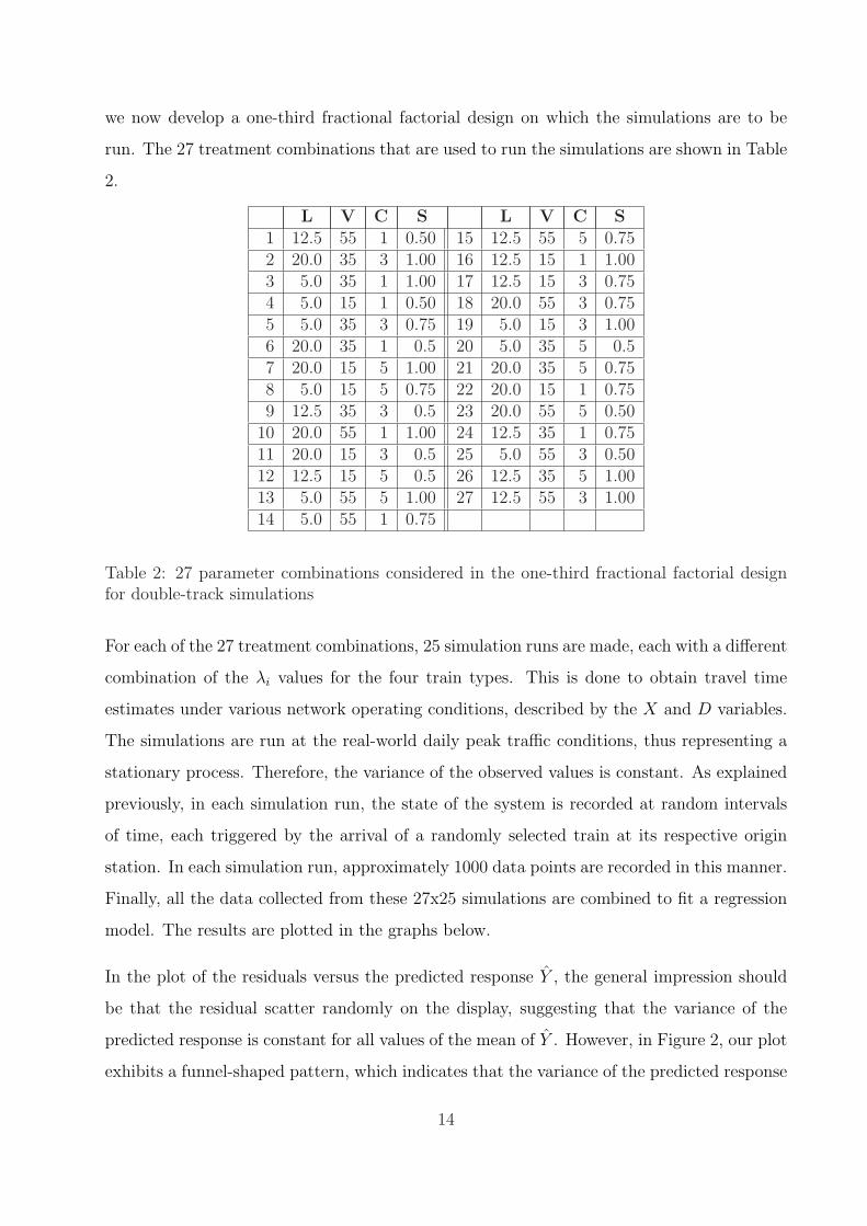
we now develop a one-third fractional factorial design on which the simulations are to be

run. The 27 treatment combinations that are used to run the simulations are shown in Table

2.

L V C S L V C S1 12.5 55 1 0.50 15 12.5 55 5 0.752 20.0 35 3 1.00 16 12.5 15 1 1.003 5.0 35 1 1.00 17 12.5 15 3 0.754 5.0 15 1 0.50 18 20.0 55 3 0.755 5.0 35 3 0.75 19 5.0 15 3 1.006 20.0 35 1 0.5 20 5.0 35 5 0.57 20.0 15 5 1.00 21 20.0 35 5 0.758 5.0 15 5 0.75 22 20.0 15 1 0.759 12.5 35 3 0.5 23 20.0 55 5 0.50

10 20.0 55 1 1.00 24 12.5 35 1 0.7511 20.0 15 3 0.5 25 5.0 55 3 0.5012 12.5 15 5 0.5 26 12.5 35 5 1.0013 5.0 55 5 1.00 27 12.5 55 3 1.0014 5.0 55 1 0.75

Table 2: 27 parameter combinations considered in the one-third fractional factorial designfor double-track simulations

For each of the 27 treatment combinations, 25 simulation runs are made, each with a different

combination of the λi values for the four train types. This is done to obtain travel time

estimates under various network operating conditions, described by the X and D variables.

The simulations are run at the real-world daily peak traffic conditions, thus representing a

stationary process. Therefore, the variance of the observed values is constant. As explained

previously, in each simulation run, the state of the system is recorded at random intervals

of time, each triggered by the arrival of a randomly selected train at its respective origin

station. In each simulation run, approximately 1000 data points are recorded in this manner.

Finally, all the data collected from these 27x25 simulations are combined to fit a regression

model. The results are plotted in the graphs below.

In the plot of the residuals versus the predicted response Y , the general impression should

be that the residual scatter randomly on the display, suggesting that the variance of the

predicted response is constant for all values of the mean of Y . However, in Figure 2, our plot

exhibits a funnel-shaped pattern, which indicates that the variance of the predicted response

14

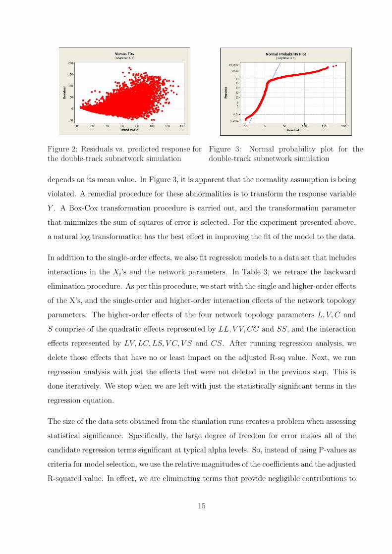
Figure 2: Residuals vs. predicted response forthe double-track subnetwork simulation

Figure 3: Normal probability plot for thedouble-track subnetwork simulation

depends on its mean value. In Figure 3, it is apparent that the normality assumption is being

violated. A remedial procedure for these abnormalities is to transform the response variable

Y . A Box-Cox transformation procedure is carried out, and the transformation parameter

that minimizes the sum of squares of error is selected. For the experiment presented above,

a natural log transformation has the best effect in improving the fit of the model to the data.

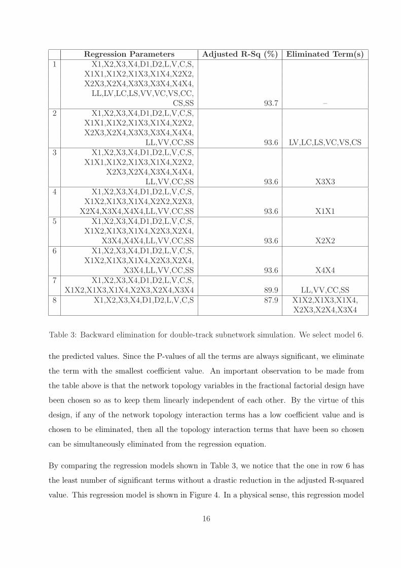
In addition to the single-order effects, we also fit regression models to a data set that includes

interactions in the Xi’s and the network parameters. In Table 3, we retrace the backward

elimination procedure. As per this procedure, we start with the single and higher-order effects

of the X’s, and the single-order and higher-order interaction effects of the network topology

parameters. The higher-order effects of the four network topology parameters L, V, C and

S comprise of the quadratic effects represented by LL, V V, CC and SS, and the interaction

effects represented by LV, LC, LS, V C, V S and CS. After running regression analysis, we

delete those effects that have no or least impact on the adjusted R-sq value. Next, we run

regression analysis with just the effects that were not deleted in the previous step. This is

done iteratively. We stop when we are left with just the statistically significant terms in the

regression equation.

The size of the data sets obtained from the simulation runs creates a problem when assessing

statistical significance. Specifically, the large degree of freedom for error makes all of the

candidate regression terms significant at typical alpha levels. So, instead of using P-values as

criteria for model selection, we use the relative magnitudes of the coefficients and the adjusted

R-squared value. In effect, we are eliminating terms that provide negligible contributions to

15

Regression Parameters Adjusted R-Sq (%) Eliminated Term(s)1 X1,X2,X3,X4,D1,D2,L,V,C,S,

X1X1,X1X2,X1X3,X1X4,X2X2,X2X3,X2X4,X3X3,X3X4,X4X4,

LL,LV,LC,LS,VV,VC,VS,CC,CS,SS 93.7 –

2 X1,X2,X3,X4,D1,D2,L,V,C,S,X1X1,X1X2,X1X3,X1X4,X2X2,X2X3,X2X4,X3X3,X3X4,X4X4,

LL,VV,CC,SS 93.6 LV,LC,LS,VC,VS,CS3 X1,X2,X3,X4,D1,D2,L,V,C,S,

X1X1,X1X2,X1X3,X1X4,X2X2,X2X3,X2X4,X3X4,X4X4,

LL,VV,CC,SS 93.6 X3X34 X1,X2,X3,X4,D1,D2,L,V,C,S,

X1X2,X1X3,X1X4,X2X2,X2X3,X2X4,X3X4,X4X4,LL,VV,CC,SS 93.6 X1X1

5 X1,X2,X3,X4,D1,D2,L,V,C,S,X1X2,X1X3,X1X4,X2X3,X2X4,

X3X4,X4X4,LL,VV,CC,SS 93.6 X2X26 X1,X2,X3,X4,D1,D2,L,V,C,S,

X1X2,X1X3,X1X4,X2X3,X2X4,X3X4,LL,VV,CC,SS 93.6 X4X4

7 X1,X2,X3,X4,D1,D2,L,V,C,S,X1X2,X1X3,X1X4,X2X3,X2X4,X3X4 89.9 LL,VV,CC,SS

8 X1,X2,X3,X4,D1,D2,L,V,C,S 87.9 X1X2,X1X3,X1X4,X2X3,X2X4,X3X4

Table 3: Backward elimination for double-track subnetwork simulation. We select model 6.

the predicted values. Since the P-values of all the terms are always significant, we eliminate

the term with the smallest coefficient value. An important observation to be made from

the table above is that the network topology variables in the fractional factorial design have

been chosen so as to keep them linearly independent of each other. By the virtue of this

design, if any of the network topology interaction terms has a low coefficient value and is

chosen to be eliminated, then all the topology interaction terms that have been so chosen

can be simultaneously eliminated from the regression equation.

By comparing the regression models shown in Table 3, we notice that the one in row 6 has

the least number of significant terms without a drastic reduction in the adjusted R-squared

value. This regression model is shown in Figure 4. In a physical sense, this regression model

16

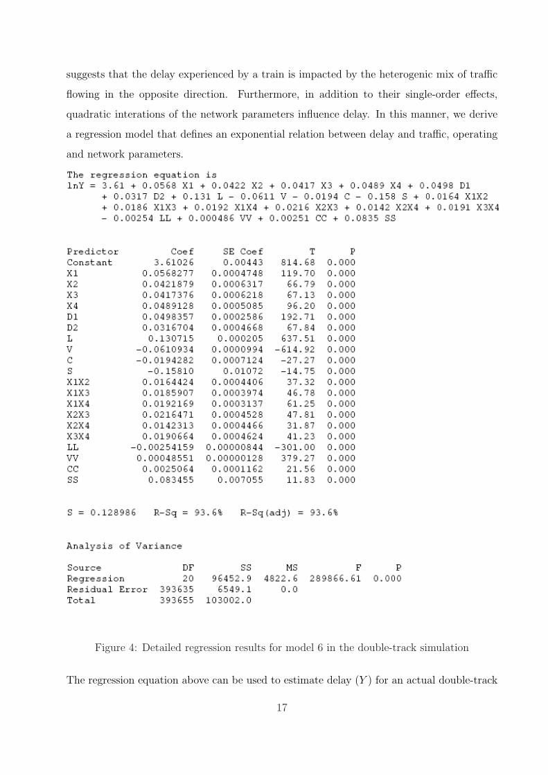
suggests that the delay experienced by a train is impacted by the heterogenic mix of traffic

flowing in the opposite direction. Furthermore, in addition to their single-order effects,

quadratic interations of the network parameters influence delay. In this manner, we derive

a regression model that defines an exponential relation between delay and traffic, operating

and network parameters.

Figure 4: Detailed regression results for model 6 in the double-track simulation

The regression equation above can be used to estimate delay (Y ) for an actual double-track

17

subnetwork.

The next logical step is to test our delay modeling methodology. As part of this step, we

adopt two validation strategies. First, we randomly chose five treatment combinations of the

54 that were not used in the one-third fractional factorial design. The performance of the

generic delay estimation model for these five network configurations is shown in rows 1-5 in

Table 4 below. In the second validation strategy, we choose a subnetwork existing in the Los

Angeles area, and test the performance of our delay estimation model on this subnetwork.

This result is shown in row 6 in Table 4 below.

L V C S Relative Error, Relative Error, Percent withinMean (%) Median (%) 20% rel. error

1 5.0 15 1 1.00 14.55 9.09 87.822 12.5 35 3 0.75 9.06 5.75 88.653 20.0 35 5 1.00 11.22 5.75 81.774 5.0 55 3 0.75 4.92 0.78 93.405 12.5 55 3 0.50 9.19 6.78 88.036 6 36.67 3 1.00 20.35 20.34 78.28

Table 4: Validation of the double-track delay model. 1-5 are from the 54 unused topologicalsubnetwork configurations. 6 is a real rail network

For a given network topology, the simulation delay values for trains are derived from running

the simulation model. The relative error is defined as the absolute value of the difference

between the simulation delay and predicted (from the delay estimation equation) delay di-

vided by the simulation delay. The mean and the median of the relative error are given

in columns 6 and 7. Our observation from these tests is that the delay estimation model

estimates data with a high accuracy under normal, expected levels of traffic. But, it also

has a tendency to overestimate delay under conditions of high traffic in a subnetwork that

could potentially lead to a deadlock. These values are small in number and, therefore, are

not removed while collecting descriptive statistics. Instead, they are considered as extreme

values. Hence, in this case, the median of the relative error proves to be a more robust

measure than the mean, and looking at the median of the relative error gives an estimate of

the effect of these extreme values on the mean of the relative error. The final column lists

the portion of the data set with a corresponding relative error within 20%, which gives an

estimate of the number of these extreme values.

18

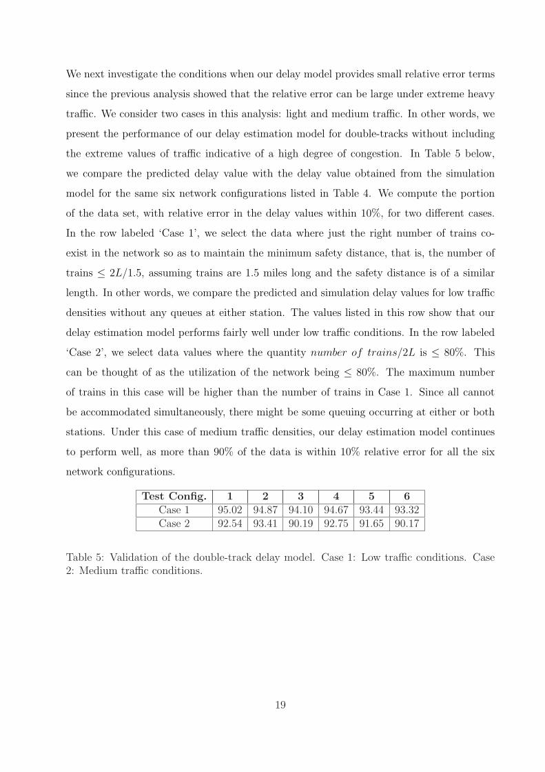
We next investigate the conditions when our delay model provides small relative error terms

since the previous analysis showed that the relative error can be large under extreme heavy

traffic. We consider two cases in this analysis: light and medium traffic. In other words, we

present the performance of our delay estimation model for double-tracks without including

the extreme values of traffic indicative of a high degree of congestion. In Table 5 below,

we compare the predicted delay value with the delay value obtained from the simulation

model for the same six network configurations listed in Table 4. We compute the portion

of the data set, with relative error in the delay values within 10%, for two different cases.

In the row labeled ‘Case 1’, we select the data where just the right number of trains co-

exist in the network so as to maintain the minimum safety distance, that is, the number of

trains ≤ 2L/1.5, assuming trains are 1.5 miles long and the safety distance is of a similar

length. In other words, we compare the predicted and simulation delay values for low traffic

densities without any queues at either station. The values listed in this row show that our

delay estimation model performs fairly well under low traffic conditions. In the row labeled

‘Case 2’, we select data values where the quantity number of trains/2L is ≤ 80%. This

can be thought of as the utilization of the network being ≤ 80%. The maximum number

of trains in this case will be higher than the number of trains in Case 1. Since all cannot

be accommodated simultaneously, there might be some queuing occurring at either or both

stations. Under this case of medium traffic densities, our delay estimation model continues

to perform well, as more than 90% of the data is within 10% relative error for all the six

network configurations.

Test Config. 1 2 3 4 5 6Case 1 95.02 94.87 94.10 94.67 93.44 93.32Case 2 92.54 93.41 90.19 92.75 91.65 90.17

Table 5: Validation of the double-track delay model. Case 1: Low traffic conditions. Case2: Medium traffic conditions.

19

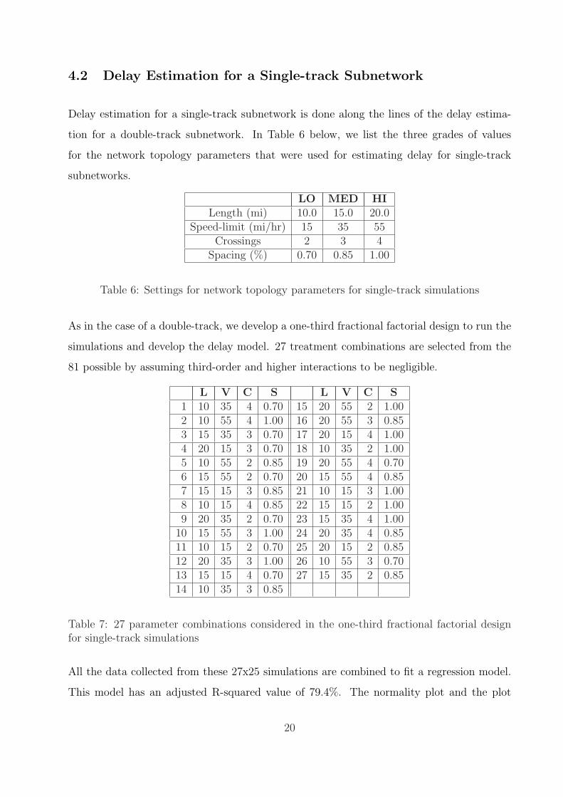
4.2 Delay Estimation for a Single-track Subnetwork

Delay estimation for a single-track subnetwork is done along the lines of the delay estima-

tion for a double-track subnetwork. In Table 6 below, we list the three grades of values

for the network topology parameters that were used for estimating delay for single-track

subnetworks.

LO MED HILength (mi) 10.0 15.0 20.0

Speed-limit (mi/hr) 15 35 55Crossings 2 3 4

Spacing (%) 0.70 0.85 1.00

Table 6: Settings for network topology parameters for single-track simulations

As in the case of a double-track, we develop a one-third fractional factorial design to run the

simulations and develop the delay model. 27 treatment combinations are selected from the

81 possible by assuming third-order and higher interactions to be negligible.

L V C S L V C S1 10 35 4 0.70 15 20 55 2 1.002 10 55 4 1.00 16 20 55 3 0.853 15 35 3 0.70 17 20 15 4 1.004 20 15 3 0.70 18 10 35 2 1.005 10 55 2 0.85 19 20 55 4 0.706 15 55 2 0.70 20 15 55 4 0.857 15 15 3 0.85 21 10 15 3 1.008 10 15 4 0.85 22 15 15 2 1.009 20 35 2 0.70 23 15 35 4 1.00

10 15 55 3 1.00 24 20 35 4 0.8511 10 15 2 0.70 25 20 15 2 0.8512 20 35 3 1.00 26 10 55 3 0.7013 15 15 4 0.70 27 15 35 2 0.8514 10 35 3 0.85

Table 7: 27 parameter combinations considered in the one-third fractional factorial designfor single-track simulations

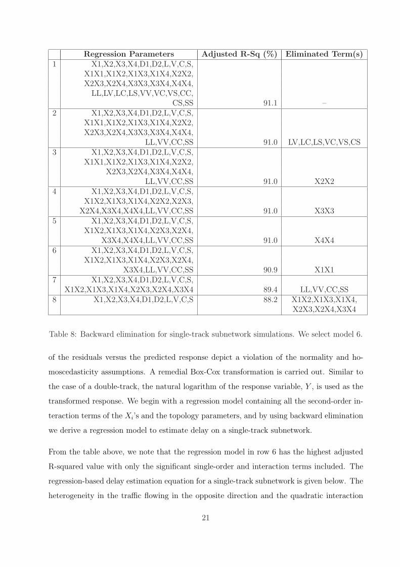
All the data collected from these 27x25 simulations are combined to fit a regression model.

This model has an adjusted R-squared value of 79.4%. The normality plot and the plot

20

Regression Parameters Adjusted R-Sq (%) Eliminated Term(s)1 X1,X2,X3,X4,D1,D2,L,V,C,S,

X1X1,X1X2,X1X3,X1X4,X2X2,X2X3,X2X4,X3X3,X3X4,X4X4,

LL,LV,LC,LS,VV,VC,VS,CC,CS,SS 91.1 –

2 X1,X2,X3,X4,D1,D2,L,V,C,S,X1X1,X1X2,X1X3,X1X4,X2X2,X2X3,X2X4,X3X3,X3X4,X4X4,

LL,VV,CC,SS 91.0 LV,LC,LS,VC,VS,CS3 X1,X2,X3,X4,D1,D2,L,V,C,S,

X1X1,X1X2,X1X3,X1X4,X2X2,X2X3,X2X4,X3X4,X4X4,

LL,VV,CC,SS 91.0 X2X24 X1,X2,X3,X4,D1,D2,L,V,C,S,

X1X2,X1X3,X1X4,X2X2,X2X3,X2X4,X3X4,X4X4,LL,VV,CC,SS 91.0 X3X3

5 X1,X2,X3,X4,D1,D2,L,V,C,S,X1X2,X1X3,X1X4,X2X3,X2X4,

X3X4,X4X4,LL,VV,CC,SS 91.0 X4X46 X1,X2,X3,X4,D1,D2,L,V,C,S,

X1X2,X1X3,X1X4,X2X3,X2X4,X3X4,LL,VV,CC,SS 90.9 X1X1

7 X1,X2,X3,X4,D1,D2,L,V,C,S,X1X2,X1X3,X1X4,X2X3,X2X4,X3X4 89.4 LL,VV,CC,SS

8 X1,X2,X3,X4,D1,D2,L,V,C,S 88.2 X1X2,X1X3,X1X4,X2X3,X2X4,X3X4

Table 8: Backward elimination for single-track subnetwork simulations. We select model 6.

of the residuals versus the predicted response depict a violation of the normality and ho-

moscedasticity assumptions. A remedial Box-Cox transformation is carried out. Similar to

the case of a double-track, the natural logarithm of the response variable, Y , is used as the

transformed response. We begin with a regression model containing all the second-order in-

teraction terms of the Xi’s and the topology parameters, and by using backward elimination

we derive a regression model to estimate delay on a single-track subnetwork.

From the table above, we note that the regression model in row 6 has the highest adjusted

R-squared value with only the significant single-order and interaction terms included. The

regression-based delay estimation equation for a single-track subnetwork is given below. The

heterogeneity in the traffic flowing in the opposite direction and the quadratic interaction

21

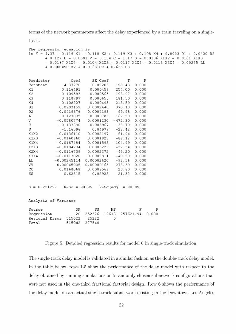
terms of the network parameters affect the delay experienced by a train traveling on a single-

track.

Figure 5: Detailed regression results for model 6 in single-track simulation.

The single-track delay model is validated in a similar fashion as the double-track delay model.

In the table below, rows 1-5 show the performance of the delay model with respect to the

delay obtained by running simulations on 5 randomly chosen subnetwork configurations that

were not used in the one-third fractional factorial design. Row 6 shows the performance of

the delay model on an actual single-track subnetwork existing in the Downtown Los Angeles

22

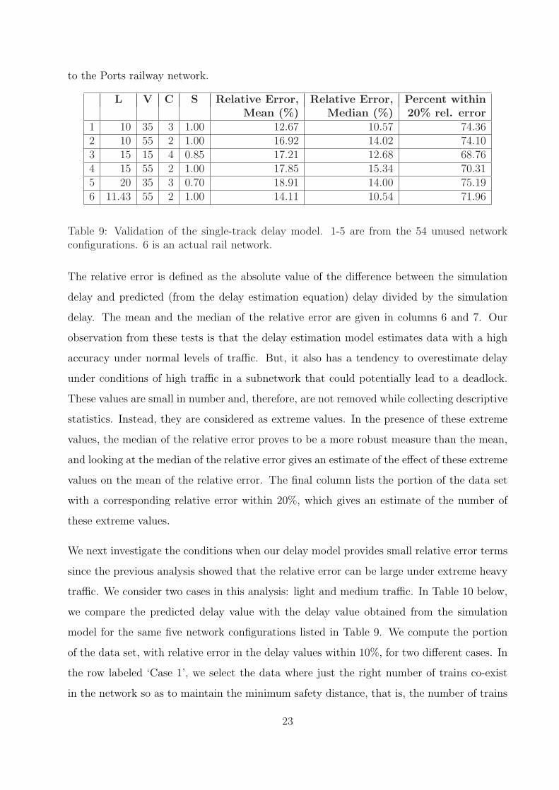
to the Ports railway network.

L V C S Relative Error, Relative Error, Percent withinMean (%) Median (%) 20% rel. error

1 10 35 3 1.00 12.67 10.57 74.362 10 55 2 1.00 16.92 14.02 74.103 15 15 4 0.85 17.21 12.68 68.764 15 55 2 1.00 17.85 15.34 70.315 20 35 3 0.70 18.91 14.00 75.196 11.43 55 2 1.00 14.11 10.54 71.96

Table 9: Validation of the single-track delay model. 1-5 are from the 54 unused networkconfigurations. 6 is an actual rail network.

The relative error is defined as the absolute value of the difference between the simulation

delay and predicted (from the delay estimation equation) delay divided by the simulation

delay. The mean and the median of the relative error are given in columns 6 and 7. Our

observation from these tests is that the delay estimation model estimates data with a high

accuracy under normal levels of traffic. But, it also has a tendency to overestimate delay

under conditions of high traffic in a subnetwork that could potentially lead to a deadlock.

These values are small in number and, therefore, are not removed while collecting descriptive

statistics. Instead, they are considered as extreme values. In the presence of these extreme

values, the median of the relative error proves to be a more robust measure than the mean,

and looking at the median of the relative error gives an estimate of the effect of these extreme

values on the mean of the relative error. The final column lists the portion of the data set

with a corresponding relative error within 20%, which gives an estimate of the number of

these extreme values.

We next investigate the conditions when our delay model provides small relative error terms

since the previous analysis showed that the relative error can be large under extreme heavy

traffic. We consider two cases in this analysis: light and medium traffic. In Table 10 below,

we compare the predicted delay value with the delay value obtained from the simulation

model for the same five network configurations listed in Table 9. We compute the portion

of the data set, with relative error in the delay values within 10%, for two different cases. In

the row labeled ‘Case 1’, we select the data where just the right number of trains co-exist

in the network so as to maintain the minimum safety distance, that is, the number of trains

23

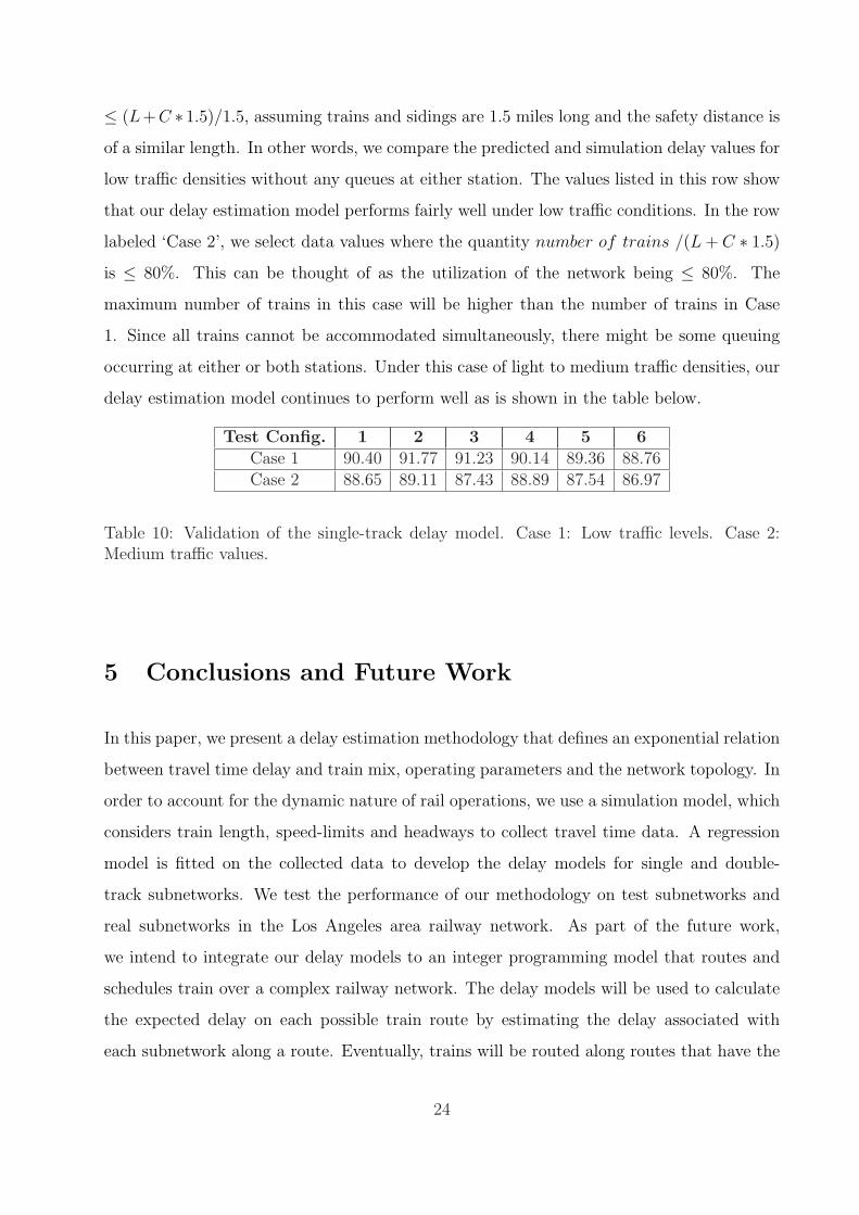
≤ (L+C ∗ 1.5)/1.5, assuming trains and sidings are 1.5 miles long and the safety distance is

of a similar length. In other words, we compare the predicted and simulation delay values for

low traffic densities without any queues at either station. The values listed in this row show

that our delay estimation model performs fairly well under low traffic conditions. In the row

labeled ‘Case 2’, we select data values where the quantity number of trains /(L + C ∗ 1.5)

is ≤ 80%. This can be thought of as the utilization of the network being ≤ 80%. The

maximum number of trains in this case will be higher than the number of trains in Case

1. Since all trains cannot be accommodated simultaneously, there might be some queuing

occurring at either or both stations. Under this case of light to medium traffic densities, our

delay estimation model continues to perform well as is shown in the table below.

Test Config. 1 2 3 4 5 6Case 1 90.40 91.77 91.23 90.14 89.36 88.76Case 2 88.65 89.11 87.43 88.89 87.54 86.97

Table 10: Validation of the single-track delay model. Case 1: Low traffic levels. Case 2:Medium traffic values.

5 Conclusions and Future Work

In this paper, we present a delay estimation methodology that defines an exponential relation

between travel time delay and train mix, operating parameters and the network topology. In

order to account for the dynamic nature of rail operations, we use a simulation model, which

considers train length, speed-limits and headways to collect travel time data. A regression

model is fitted on the collected data to develop the delay models for single and double-

track subnetworks. We test the performance of our methodology on test subnetworks and

real subnetworks in the Los Angeles area railway network. As part of the future work,

we intend to integrate our delay models to an integer programming model that routes and

schedules train over a complex railway network. The delay models will be used to calculate

the expected delay on each possible train route by estimating the delay associated with

each subnetwork along a route. Eventually, trains will be routed along routes that have the

24

least expected delay. To route and schedule trains over a large complex network can be

computationally intensive. One way to reduce complexity could be to “aggregate” suitable

sections of a network. We have developed a model presented in this paper for this purpose.

In addition to this, our delay estimation procedure has an advantage of being able to easily

integrate with a routing and scheduling integer programming model.

Efficient delay estimation and capacity assessment techniques are cost-effective ways to re-

lieve rail network congestion. These methods allow railway planners to dispatch just the

right number of trains that can be handled by a network without resulting in a deadlock,

while maintaining travel time delays to a minimum. Dispatchers can use the delay estima-

tion procedure presented in this paper to study how the delay in the aggregated section of

the network varies with each additional train. Once a delay estimation equation has been

generated by our technique, it can be used to estimate delay and capacity of a network

with physical attributes within the upper and lower limits of the attributes of the generic

networks used in the experiments. That is, individual simulations need not be run for every

aggregated network section.

25

References

[1] Burdett, R. L., and Kozan, E. Techniques for absolute capacity determination in

railways. Transportation Research Part B 40 (2006), 616–632.

[2] Carey, M., and Kwiecinski, A. Stochastic approximation to the effects of headways

on knock-on delays of trains. Transportation Research Part B 28B(4) (1994), 251–267.

[3] Chen, B., and Harker, P. T. Two moments estimation of the delay on a single-track

rail line with scheduled traffic. Transportation Science 24 (1990), 261–275.

[4] D’Ariano, A. Improving Real-time Train Dispatching: Models, Algorithms and Ap-

plications, t2008/6 ed. TRAIL Thesis Series, The Netherlands, 2008.

[5] de Kort, A. F., Heidergott, B., and Ayhan, H. A probabilistic (max,+) ap-

proach for determining railway infrastructure capacity. European Journal of Operational

Research 148 (2003), 644–661.

[6] Dessouky, M. M., and Leachman, R. C. A simulation modeling methodology for

analyzing large complex rail networks. Simulation 65:2 (1995), 131–142.

[7] Frank, O. Two-way traffic in a single line of railway. Operations Research 14 (1966),

801–811.

[8] Gibson, S., Cooper, G., and Ball, B. Developments in transport policy: The

evolution of capacity charges on the uk rail network. Journal of Transport Economics

and Policy 36 (2002), 341–354.

[9] Greenberg, B. S., Leachman, R. C., and Wolff, R. W. Predicting dispatching

delays on a low speed, single tack railroad. Transportation Science 22(1) (1988), 31–38.

[10] Hallowell, S. F., and Harker, P. T. Predicting on-time line-haul performance

in scheduled railroad operations. Transportation Science 30 (1996), 364–378.

[11] Harker, P. T., and Hong, S. Two moments estimation of the delay on a partially

double-track rail line with scheduled traffic. Transportation Research Forum 30 (1990),

38–49.

26

[12] Higgins, A., and Kozan, E. Modeling train delays in urban networks. Transportation

Science 32(4) (1998), 251–356.

[13] Huisman, T., and Boucherie, R. J. Running times on railway sections with het-

erogeneous train traffic. Transportation Research Part B 35 (2001), 271–292.

[14] Kaas, A. H. Methods to Calculate Capacity of Railways. PhD thesis, Dept. of Planning,

Technical University of Denmark, 1998.

[15] Krueger, H. Parametric modeling in rail capacity planning. Proceedings of the Winter

Simulation Conference, pp. 1194–1200.

[16] Landex, A., Kaas, A. H., and Hansen, S. Railway operation. Report 4, Centre

for Traffic and Transport, Technical University of Denmark, 2006.

[17] Leachman, R. C. Inland empire railroad main line advanced planning study. Tech.

rep., Prepared for the Southern California Association of Governments, Contract num-

ber 01-077, Work element number 014302, October 1, 2002.

[18] Lu, Q., Dessouky, M. M., and Leachman, R. C. Modeling of train movements

through complex networks. ACM Transactions on Modeling and Computer Simulation

14 (2004), 48–75.

[19] Montgomery, D. C. Design and Analysis of Experiments, 2nd ed. John Wiley and

Sons, 1984.

[20] Myers, R. H., and Montgomery, D. C. Response Surface Methodology, 2nd ed.

Wiley Series in Probability and Statistics, 2002.

[21] Ozekici, S., and Sengor, S. On a rail transportation model with scheduled services.

Transportation Science 28(3) (1994), 246–255.

[22] Petersen, E. R. Over the road transit time for a single track railway. Transportation

Science 8 (1974), 65–74.

[23] Petersen, E. R., and Taylor, A. J. A structured model for rail line simulation

and optimization. Transportation Science 16 (1982), 192–206.

27

[24] Pritsker, A. A. B., and O’Reilly, J. J. Simulation with Visual SLAM and

AweSim, 2nd ed. John Wiley and Sons, New York and Systems Publishing Corporation,

West Lafayette, Indiana, 1999.

[25] Wendler, E. The scheduled waiting time on railway lines. Transportation Research

Part B 41 (2007), 148–158.

[26] Yuan, J. Stochastic Modeling of Train Delays and Delay Propagation in Stations. Ph.D

Thesis, Delft University of Technology, The Netherlands, 2006.

[27] Yuan, J., and Hansen, I. A. Optimizing capacity utilization of stations by estimating

knock-on train delays. Transportation Research Part B 41 (2007), 202–217.

28