a data base for the u.s. forest service pavement
TRANSCRIPT

A DATA.BASE FOR THE U.S. FOREST SERVICE
PAVEMENT MANAGEMENT SYSTEM
Jorge E. Hernan~~z, B. Frank McCullough, and W. Ronald Hudson
r·
TRANSPORTATION RESEARCH REPORT 66
CENTER FOR TRANSPORTATION RESEARCH BUREAU OF ENGINEERING RESEARCH
THE UNIVERSITY OF TEXAS AT AUSTIN
MAY 1981
CTR66

PARTIAL LIST OF REPORTS PUBLISHED BY THE CENTER FOR TRANSPORTATION RESEARCH
This list includes some of the reports published by the Center for Transportation Research and the organizations which were merged to form it: the Center for Highway Research and the Council for Advanced Transportation Studies. Questions about the Center and the availability and costs of specific reports should be addressed to: Director; Center for Transportation Research; ECl 2.5; The University of Texas at Austin; Austin, Texas 78712.
7·1
7·2F
16-IF 23·1
23·2
23·3F
29·2F
114-4
114-5
114-6
114-7
114-8 114·9F 118·9F
123·30F
172·1 I 72-2F 176·4 176-5F 177·1
177-3
177-4
177-6
177·7
177·9
177·10
177·11
177·12
177·13
177·15
177·16 177·17 177·18
183·7
"Strength and Stiffness of Reinforced Concrete Rectangular Columns Under BiaxiaUy Eccentric Thrust," by J. A. Desai and R. W. Furlong, January 1976. "Strength and Stiffness of Reinforced Concrete Columns Under Biaxial Bending," by V. Mavichak and R. W. Furlong, November 1976. "Oil, Grease, and Other Pollutants in Highway Runoff," by Bruce Wiland and Joseph R Malina, Jr., September 1976. "Prediction of Temperature and Stresses in Highway Bridges by a Numerical Procedure Using Daily Weather Reports," by Thaksin Thepchatri, C. Philip Johnson, and Hudson Matlock, February 1977. "Analytical and Experimental Investigation of the Thermal Response of Highway Bridges," by Kenneth M. Will, C. Philip Johnson, and Hudson Matlock, February 1977. "Temperature Induced Stresses in Highway Bridges by Finite Element Analysis and Field Tests," by Atalay Yargicoglu and C. Philip Johnson, July 1978. "Strength and Behavior of Anchor Bolts Embedded Near Edges of Concrete Piers," by G. B. Hasselwander, J, O. Jirsa, J. E. Breen, and K. Lo, May 1977. "Durability, Strength, and Method of Application of Polymer·Impregnated Concrete for Slabs," by Piti Yimprasert, David W. Fowler, and Donald R. Paul, January 1976. "Partial Polymer Impregnation of Center Point Road Bridge," by Ronald Webster, David W. Fowler, and Donald R. Paul, January 1976. "Behavior of Post·Tensioned Polymer·Impregnated Concrete Beams," by Ekasit Limsuwan, David W. Fowler, Ned H. Burns, and Donald R. Paul, June 1978. "An Investigation of the Use of Polymer·Concrete Overlays for Bridge Decks," by Huey· Tsann Hsu, David W. Fowler, Mickey Miller, and Donald R. Paul, March 1979. "Polymer Concrete Repair of Bridge Decks," by David W. Fowler and Donald R. Paul, March 1979. "Concrete· Polymer Materials for Highway Applications," by David W. Fowler and Donald R. Paul, March 1979. "Observation of an Expansive Clay Under Controlled Conditions," by John B. Stevens, Paul N. Brotcke, Dewaine Bogard, and Hudson Matlock, November 1976. "Overview of Pavement Management Systems Developments in the State Department of Highways and Public Transportation," by W. Ronald Hudson, B. Frank McCullough, Jim Brown, Gerald Peck, and Robert L. Lytton, January 1976 (published jointly with the Texas State Department of Highways and Public Transportation and the Texas Transportation Institute, Texas A&M University). "Axial Tension Fatigue Strength of Anchor Boits," by Franklin L. Fischer and Karl H. Frank, March 1977. "Fatigue of Anchor Bolts," by Karl H. Frank, July 1978. "Behavior of Axially Loaded Drilled Shafts in Clay·Shales," by Ravi P. Aurora and Lymon C. Reese, March 1976. "Design Procedures for Axially Loaded Drilled Shafts," by Gerardo W. Quiros and Lymon C. Reese, December 1977. "Drying Shrinkage and Temperature Drop Stresses in Jointed Reinforced Concrete Pavement," by Felipe Rivero· Vallejo and B. Frank McCullough, May 1976. "A Study of the Performance of the Mays Ride Meter," by Yi Chin Hu, Hugh J. Williamson, and B. Frank McCullough, January 1977. "Laboratory Study of the Effeci of Nonuniform Foundalion Support on Continuously Reinforced Concrele Pavements," by Enrique Jimenez, B. Frank McCullough, and W. Ronald Hudson, August 1977. "Sixteenth Year Progress Report on Experimental Continuously Reinforced Concrete Pavement in Walker County," by B. Frank McCullough and Thomas P. Chesney, April 1976. "Continuously Reinforced Concrete Pavement: Structural Performance and Design/Construction Variables," by Pieter J. Strauss, B. Frank McCullough, and W. Ronald Hudson, May 1977. "CRCP·2, An Improved Computer Program for the Analysis of Continuously Reinforced Concrete Pavements," by James Ma and B. Frank McCullough, August 1977. "Development of Photographic Techniques for Performing Condition Surveys," by Pieter Strauss, James Long, and B. Frank McCullough, May 1977. "A Sensitivity Analysis of Rigid Pavement Overlay Design Procedure," by B. C. Nayak, W. Ronald Hudson, and B. Frank McCullough, June 1977. "A Study of CRCP Performance: New Construction Vs. Overlay," by James I. Daniel, W. Ronald Hudson, and B. Frank McCullough, April 1978. "A Rigid Pavement Overlay Design Procedure for Texas SDHPT," by Otto Schnitter, W. R. Hudson, and B. F. McCullough, May 1978. "Precast Repair of Continuously Reinforced Concrete Pavement," by Gary Eugene Elkins, B. Frank McCullough, and W. Ronald Hudson, May 1979. "Nomographs for the Design ofCRCP Steel Reinforcement," by C. S. Noble, B. F. McCullough, and J. C. M. Ma, August 1979. "Limiting Criteria for the Design ofCRCP," by B. Frank McCullough, J. C. M. Ma, and C. S. Noble, August 1979. "Detection of Voids Underneath Continuously Reinforced Concrete Pavements," by John W. Birkhoff and B. Frank McCullough, August 1979. "Permanent Deformation Characteristics of Asphalt Mixtures by Repeated-Load Indirect Tensile Test," by Joaquin Vallejo, Thomas W. Kennedy, and Ralph Haas, June 1976.
(Continued inside back caver)

A DATA BASE FOR THE U. S. FOREST SERVICE
PAVEMENT MANAGEMENT SYSTEM
by
Jorge E. Hernandez B. Frank McCullough
W. Ronald Hudson
THE CENTER FOR TRANSPORTATION RESEARCH
THE UNIVERSITY OF TEXAS AT AUSTIN
May 1981

!!!!!!!!!!!!!!!!!!!"#$%!&'()!*)&+',)%!'-!$-.)-.$/-'++0!1+'-2!&'()!$-!.#)!/*$($-'+3!
44!5"6!7$1*'*0!8$($.$9'.$/-!")':!

Background
AN EXECUTIVE SUMMARY of
the report
A PAVEMENT DATA BASE FOR PDMS
by
Jorge E. Hernandez B. Frank McCullough
W. Ronald Hudson
This report is the first phase of a proposed three-phase project developing and impleme~ting a data base for the Pavement Design Management System (PDMS) which was developed by The University of Texas Austin in cooperation with the U.S. Forest Service.
for and at
PDMS may be used to design asphalt concrete, surface treatment, and aggregate surfaced pavement structures. Results from the implementation of PDMS in certain Forest Service design offices indicate good performance of PDMS regarding the asphalt concrete and surface treatment pavement designs. However, the implementation results also indicate that the models used in PDMS for the design of aggregate surfaced roads need to be improved. This is not surprising, since these models were not developed with data from Forest Service roads.
The characteristics of the Forest Service road system make it truly unique in the world. Because of this, roadway structure design and management methodologies developed by other transportation agencies are not adequate for Forest Service needs. To improve these methodologies in PDMS, performance information on Forest Service roads must be collected and analyzed. Even a small improvement in the management of pavement structures system-wide will result in the saving of millions of dollars annually. Therefore, a data base is a necessary and valuable tool.
Scope of Report
The feasibility of such a data base is analyzed in this report. Three major parts may be identified in the report. The first part, including Chapters 1, 2, and 3, deals with problem identification and selection of the variables to be included in the data base. The second part, including Chapters 4 and 5, deals with the description and evaluation of the procedures, devices, and methods that may be used for collecting the
iii

information. The third part, Chapter 6, deals with the design of the experiment for collecting pavement performance information regarding aggregate surfaced roads and unsurfaced roads. Three experiment alternatives are generated by considering different numbers of test sections as well as a time duration of observations. A rough cost estimate is also presented in Chapter 6.
Chapter 7 presents the conclusions and recommendations derived from the report.
Results From Questionnaire
In order to develop the necessary background information for data base recommendations, a "Forest Characterization Questionnaire" was sent to all the National Forests. The questionanaire's intent was to characterize the National Forest in terms of road mileage, type of surface, number of lanes, pavement structural characteristics (number of layers and thicknesses), traffic volume and classification, and tOPGgraphic and environmental parameters, as well as material testing methods and traffic measuring systems.
Of 140 questionnaires sent, 83 percent were completed and returned. The information included was summarized in a national summary, presented in Appendix B, as well as in one regional summary for each of the regions of the Fbrest Service. The information presented in these summaries is based on the received information, and no adjustment factor was used to extrapolate from 83 percent of the completed questionnaires to 100 percent of the mailed questionnaires.
Some of the important facts derived from this survey are that the U.S. Forest Service road network is more than 248,000 miles long, with almost 68 percent of the roads classified as unsurface9 roads, 28 percent as aggregate surfaced roads, and less than 5 percent as asphalt concrete or surface treatment roads. It is also interesting that Region 6 (primarily Oregon and Washington) has almost 30 percent of the roads under the Forest Service administration and that 90 percent of the roads are "one-lane" roads. Other interesting facts are that 70 percent of the aggregate surfaced roads have a traffic volume of less than 50 vehicles per day, and almost 90 percent of the aggregate surfaced roads have less than 100 vehicles per day. Additional detailed information is presented in Chapter 2 of the report.
Description of Date Base Experiment
As a result of the analysis performed in Chapter 3 to identify the variables for inclusion in the data base, we recommend the measurement of four major pavement performance variables, namely, rut depth, roughness, aggregate loss, and looseness. These four variables are designated dependent variables and they indicate in one way or another a measure of pavement performance.
iv
•

Variation of these variables depends upon the combination of a set of secondary variables, namely, traffic, pavement thickness, pavement materials, and environmental and topographical factors. These secondary variables are designated independent variables.
It is proposed that these dependent and monitored in the Primary Study, which would continental United States.
independent variables be be conducted across the
A second set of studies, known as Satellite Studies, are proposed to determine the influence of specific factors on pavement condition in a more limited sphere. Two satellite studies are proposed for both aggregate surfaced and unsurfaced roads to study the effect of different maintenance levels and the freeze-thaw cycle on the pavement condition.
Equipment, procedures, and methods for measuring each of the dependent and independent variables are described and evaluated in Chapters 4 and 5. It is recommended that, prior to any decision as to methodology, a pilot study be conducted in order to verify the performance, adequacy, and cost for the proposed devices, procedures, and methods. Recommendations on performing this pilot study are presented in Chapters 6 and 7. The sections selected for the Pilot Study can eventually be included in the pavement data base; therefore, all the information will be utilized.
Several alternative designs for the data base are presented in Chapter 6; one set of alternatives was developed for aggregate surfaced roads and one set for unsurfaced roads. In both cases, the alternatives were generated by varying the total number of test sections. Also, three time durations have been considered: one, two, and three years. The proposed alternatives have a statistical basis developed from the methodology for the design of experiments, which is briefly described in Chapter 6.
Cost of Date Base Experiment
A rough estimate of the experiment cost for each of the proposed alternatives has been determined. For the case of aggregate surfaced roads, it is as follows:
Experiment A Duration (198*)
One year $3,888,000
Two years 6~047,000
Three years 8,,205,000
B
J;1.26*)
$2,441,000
3,908,000
c (54*)
$.993,000
1,770,000
2,547,000
*The number in parenthesis refers to the number of test sections.
v

For the case of unsurfaced roads, the cost for each experiment alternative is as follows:
EXEeriment Alternatives Experiment A B C Duration (198*) (126*) (54*~
One year $3,888,000 $2,441,000 $ 993,000 Two years 6,047,000 3,908,000 1,770,000 Three years 8,205,000 5,376,000 2,547,000
*The number in parenthesis refers to the number of test sections.
From the previous figures, it may be noted that the least expensive alternative calls for 54 sections of aggregate surfaced roads and 16 test sections of unsurfaced roads for a duration of one year. The cost of such an alternative would be $1,230,000.
At the other extreme, if it is decided to collect information over a period of three years, establishing 198 sections for aggregate surfaced roads and 76 sections for unsurfaced roads, the cost would be $10,798,000, almost ten times the previous figure. However, with the benefits of improved pavement structure design and maintenance, as well as more accurate information for planning and estimating purposes, this data base cost could be rapidly exceeded by the benefits. Conaidering annual maintenance costs alone, a savings of only a few percent would result in millions of dollars in reduced cost annually.
The cost of a Pilot Study can be fixed at a given level and the number of test sections varied to fit the budget. It is recommended that the budget be set at a level of $175,000 to $200,000.
Decision Considerations
In making the· final decision regarding the experiment layout, we recommend that the Forest Service Administration keep in mind the reliability of information derived from each of the alternatives. Obviously, the more test sections, the more reliable the derived models, conclusions, etc. Care should be exercised not to make arbitrary decisions based strictly on a first cost criteria. Such decisions may produce an experiment with less useful information and, conse~uently, less applicability.
vi

When making a final decision, the present investment in the Forest Service road network, as well as the magnitude of this road network should be considered. The Forest Service Transportation System is much larger than the road network in most countries. In addition, Forest Service roads have ax~e loadings, seasonal traffic variations, environmental conditions, topographic constraints, and surfacing materials that as a whole, are different than any other transportaton agency in the world. Important information applicable to Forest Service roads will not be available from any other source. These facts suggest the study be performed at as high a level as possible.
Considering the annual appropriated expenditures in regular maintenance, Which in 1980 was $77 million, the least expensive experiment alternative IBpresents 1.6 percent of this 'figure. Assuming that 5 percent of the annual maintenance expenditures would be saved with the operation of an efficient POMS, then the cost of the least expensive experiment would have a payback period of approximately one-third of a year.
If the most expensive experiment layout is selected and measurements are made over a period of three years, the experiment cost would be around $11 million, or $3.7 million annually. This annual figure represents only 4.8% of the maintenance expenditures appropriated in 1980.
Another fact that may influence the final decision is the worldwide lack of reliable and adequate information regarding the performance of aggregate surfaced roads and unsurfaced roads. With more than 95 percent of the Forest Service road system miles in this category, better information is extremely important_
The availability of adequate information would allow a definition of optimum pavement design and maintenance policies, which should lead to an optimum utilization of the available resources. In the same way, this information should lead to more uniformity of policies among the various Forest Service offices, which is another factor to be considered when the final decision relating to the development of the data base for PDMS is made.
vii

TABLE OF CONTENTS
AN EXECUTIVE SUMMARY OF THE REPORT • • • • • . • • • • • • • • • • • • • iii
CHAPTER 1. INTRODUCTION AND BACKGROUND
Forest Service Road Network • • • • • • • • Development of the PDMS Computer Program Components of PDMS ••••••• The Need for a PDMS Data Base • • • • Objectives and Scope of the Study .
CHAPTER 2. FOREST CHARACTERIZATION QUESTIONNAIRE
Background • • • • Summary of Data • • • • •
CHAPTER 3. IDENTIFICATION AND SELECTION OF THE VARIABLES TO BE MEASURED
Brainstorming Session • • • • . • . . • . • . • • Sensitivity Analysis of the PDMS Computer Program C.T., Coghlan Questionnaire for Aggregate Surfaced The Kenya Study . • • •• • . •••• The Brazil Study • • . • • Recommended Study Variables • . • • • • • • • .
Roads
CHAPTER 4. REVIEW AND SELECTION OF THE METHODS TO MEASURE DEPENDENT VARIABLES
Rut Depth Measurements Roughness Measurements . • . • Aggregate Loss Measurements • . . • • Looseness of Material Measurements
CHAPTER 5. REVIEW AND SELECTION OF THE METHODS TO MEASURE INDEPENDENT VARIABLES
Mate~ial Properries • • • • • . Layer Thickness Measurements • • • • Traffic Measurement • • • • • • • • . Environmental Factor • • • • •
viii
1 5 6
10 13
17 19
50 51 56 58 62 63
67 76 95
• • 106
• • 111 • 121 • 124
• • 135

CHAPTER 6. DESIGN OF THE SAMPLING PLAN
The Design of Experiments • • • • • • • • • • Experiment on the Performance of Aggregate Surfaced Roads • Experiment on the Performance of Unsurfaced Roads • • Cost Analysis • • • • • Pilot Study • •• • • • • . • • • •
CHAPTER 7. CONCLUSIONS AND RECOMMENDATIONS
Conclusions • • • 0 • • • • 0
Study Recommendations . • • Pilot Study Recommendations
REFERENCES
APPENDICES
Appendix A.
Appendix B.
Appendix Co Appendix D. Appendix E. Appendix F. Appendix G. Appendix H. Appendix Io
Forest Characterization Questionnaire, List of National Forests and Data Processing Information Forest Characterization Questionnaire, National Summ.ary .••.. • • • • . • . • • . • Sunnnary of the "Brainstorming Session" • PCA Road Meter Measurement Variability Mays Meter Variability 0 • 0 0 0 • 0
Mays Meter Calibration Procedures Deflection Measurement Devices Vehicle Load Weighers Cost Analysis 0.... 0 0 0
ix
• 0 • 143 o 144
• 0 153 o 154 o 162
• • 163 o 0 164 • • 165
• • 167
• 175
o 0 • 197 • 241
• • 253 o 257
o 0 265 • 273 • 281 • 291

!!!!!!!!!!!!!!!!!!!"#$%!&'()!*)&+',)%!'-!$-.)-.$/-'++0!1+'-2!&'()!$-!.#)!/*$($-'+3!
44!5"6!7$1*'*0!8$($.$9'.$/-!")':!

CHAPTER 1. INTRODUCTION AND BACKGROUND
Under the terms of a coooperative agreement, The University of Texas and the U.S. Forest Service have been working together to develop a pavement management system applicable to the roads under the Forest Service jurisdiction. This pavement management system, known as the Pavement Design and Management System (PDMS), was implemented in 1979 in selected Forest Service design offices, and is being integrated as a part of the Forest Service Road Design Handbook.
In order to expand and improve the capabilities of PDMS, more development is necessary. Nearly all of the mathematical models used in PDMS m determine road surfacing strategies were developed by agencies other than the U.S. Forest Service. This is because almost no information on the performance of Forest Service roads has ever been systematically collected, especially in the relatively unexplored area of aggregate surfaced and unsurfaced roads. To properly gather this information, a data base for monitoring the performance of Forest Service roads is vital. The purpose of this project is to perform a feasibility study for such a data base.
Chapter 1 provides background information; the Forest Service Road Network is delineated, and a brief description of PDMS is included. General concepts about the functions and purpose of a data base in any pavement management system are outlined. Finally, the approach adopted to perform this feasibility study is defined.
FOREST SERVICE ROAD NETWORK
The Forest Service, as a division of the U.S. Department of Agriculture, is responsible for the wise use of forests and related watershed lands. These lands comprise, as stated by Howlett, (Ref 1), one third of the total land area of the United States. A significant part of this land area, approximately 750,000 km (187 million acres), is under direct Forest Service management. The Forest Service is organized in nine regions, which include 155 National Forests and 19 National Grasslands, located in 44 states and Puerto Rico (Fig 1.1).
The lands administered by the Forest Service are managed for different purposes:
1

Q
.. --.-.
. -.. -,
,-.. ~ .. -
Ho.
rHII.
Ir&
IOH
(I)~' ~
• II
. O
AK
. M
ON
T.
!.:.'::
.. ~:..~
. ....
b~_
NE
BR
.
'l
) II
INIi
. S
_~,.
r._
.1
-, .
......
;--
10C
lY
.0U
N,a
'N
f If"
ON
·(ij-·-
~-.
[-=:
~ -'V
lno
.te
.
'. '"
I i
l. /'._
.. ""-,,
'\
KA
NS
.
TE
XA
S
..::.. ..
/,,/\
( .
i \.
. )
ll~'
-l
/-'-"-"'~
:'
\ ,,
't)
.~ ..
/
-'I
..,.
...
~.
~':.
1,1.
-,
\"~
.'_-II
ICII~Y
,
-." ~.~
p
•
--T
' :.~
,f
2.:;
;~-
usn •
•• (G
IO.
\91
\ P
" \
0111
0 ~
INO
. \
.
'-..
NAT
ION
AL F
ORE
ST S
YSTE
M
AND
R
ElA
TE
D D
ATA
a.-
, ....
.. fO
IIIw
n
-~ ... .
. c:
::J _,~ ..
....
L",.,..
~ ~ Y
TL
lzau
,. N
O"C
" -
........ .
.,...,..
... .. •
• ..
au..
. oC
oI.A
IOU
oUU
Itl
Fig
1.1
. E
xte
nt
and
lo
cati
on
of
Fo
rest
S
erv
ice
lan
ds
(Ref
1
).
N

(1) Timber production,
(2) Watershed protection,
(3) Forage prOduction,
(4) Wildlife habitat improvement, and
(5) Recreation.
3
Some of the most important activities carried out by the Forest Service are: reforestation, timber stand improvement, revegetation, range improvement, land acquisition and land exchange, recreation, control of forest fires, etc. In order to carry out these activities, the U.S. Forest Service manages an impressive and complex road system, which is more than 250,000 miles long and may be classified by surface type as follows:
Surface Type IDln %
Asphalt concrete 5,864 2.4
Surface treatment 5,922 2.4
Aggregate surfaced roads 68,741 27.7
Unsurfaced roads 167,408 67.5
Total 247,935 100.0
These data were developed based on the information presented in Chapter 2.
Table 1.1 provides an idea of the magnitude and importance of the Forest Service road network by comparing it with road networks of some countries. Note that the U.S. Forest Service network is in sixth place on a length basis.
The complexity of the road system operated by the Forest Service is increased by the existence of trails, ski lifts, cable logging facilities, yarding areas, airfields, heliports, boat ramps, and boat docking facilities. These facilities imply the movement of people and goods, and consequently, the existence of roads. There will exist a great variety of users of these roads. One of the largest groups of users are the haulers of wood products. Frequently heavy trucks are used, producing high stresses in the road surfacings. However, the number of repetitions is relatively small. Among the other users of these roads are: residents of private lands within the

~
TABL
E 1
.1.
ROAD
NE
TWOR
K IN
SO
ME
COU
NTR
IES
(REF
7
1).
Len
gth
of
Len
gth
of
Unp
aved
Len
gth
Co
un
try
P
aved
Roa
ds
Unp
aved
R
oads
T
ota
l T
ota
l L
eng
th
(km
) (k
m)
(km
)
Un
ited
S
tate
s 3
,15
3,0
32
3
,06
9,1
90
6
,22
2,2
22
0
.49
Bra
zil
80
,202
1
,46
4,4
82
1
,54
4,6
84
0
.95
Fra
nce
90
2,84
9 5
31
,45
8
1,4
34
,30
7
0.3
7
Jap
an
405,
353
68
2,9
01
1
,08
8,2
54
0
.63
Wes
t G
erm
any
412,
700
62
,30
0
47
5,0
00
0
.13
U.
S.
Fo
rest
Ser
vic
e 1
8,9
64
37
9,96
6 3
98
,93
0
0.9
5
Sp
ain
1
53
,17
8
16
6,8
50
3
20
,02
8
0.5
2
Arg
enti
na
47,5
50
16
0,5
37
2
08
,08
7
0.7
7
Mex
ico
62,9
56
14
4,2
39
2
07
,19
5
0.7
0
So
uth
Afr
ica
52
,50
5
14
3,3
94
1
95
,89
9
0.7
3
Net
her
lan
ds
86
,30
0
18
,13
0
10
4,4
30
0
.17
Irela
nd
87
,422
4
,87
2
92
,29
4
0.0
5
Ken
ya
4,4
76
4
6,0
34
5
0,5
10
0
.91
Bo
liv
ia
1,1
63
3
6,1
55
3
7,3
18
0
.97
1 km
= 0
.62
15
mil
es

5
National Forests, recreationalists, ore haulers, and forest administrators. These roads must accommodate a mixture of vehicles similar to most public road systems.
Another important characteristic of this road network is the distribution of traffic throughout the year. There will be periods of the year when the roads may not be widely used and others, like the hunting and fishing seasons, weekends, summer camping, winter skiing season or accelerated timber salvage sales, when the number of vehicles per day will be very large.
The environmental factors, such as heavy precipitation and spring thaw, Play an important role in the design, construction, and operation of these unpaved roads. Such conditions may either make a road impassable or may force temporary road closure. These situations rarely occur in the paved s.ystems. The design speeds on Forest Service roads are generally less than 48 kmh (30 mph), and a great portion of the roads were constructed as long as 75 years ago, reflecting chronological changes as well as political and mission oriented changes. Many of the roads were neither designed nor engineered, but were developed from earlier routes such as Indian trails and animal paths.
The investment in the existing Forest Service road system is approximately $2,500 million. About 16,000 km are constructed and reconstructed annually, representing an additional annual investment of more than $272 million. In 1980, Forest Service maintenance expenditures for the road system were about $77 million.
Clearly, the size of the Forest Service road system, as well as the predominent use of unbound surfacing materials, sets it apart from other transportation agencies in the U. S.. Considering the additional factors of heavy axle loads, seasonal traffic variations, extreme environmental conditions, and low-volume traffic, the Forest Service road system is truly unique in the world. It is difficult, therefore, to design and manage the roadway structure of this system using methodologies and data from other transportation agencies.
It will be necessary to develop a Forest Service data base to be able to develop optimum design and maintenance procedures for Forest Service roads.
DEVELOPMENT OF THE PDMS COMPUTER PROGRAM
Management of such a unique and complex road network as that of the U.S. Forest Service is not an easy task. In addition to the factors previously mentioned, other aspects such as organizational constraints and organizational acceptance, must be considered. The interaction of these parameters presents a situation that requires the optimum use of material, financial, and human resources in order to satisfy maximum needs in the most reasonable way.

6
In order to properly face this challenge, the U.S. Forest Service and The University of Texas initiated a cooperative study in 1972 to develop a pavement management system for the Forest Service road network. The work has been conducted in three phases under the project name, "A Pavement Design and Management System for Forest Service Roads." As of today, three reports have been produced as follows:
Phase I "A Conceptual Study" July 1974
Phase II "A Working Model" February 1977
Phase III "Implementation" January 1979
During Phase I, the feasibility of developing such a pavement management system was analyzed. The positive results obtained from this research led to the development of a working computer based model during Phase II of the project. The working model is known as PDMS (Pavement Design and Management System). In the "Implementation" report, (Phase III), the experience derived from a trial implementation in several offices of the Forest Service was presented. As a result of this third phase, two additional projects have been conducted at The University of Texas. The first of these is known as "Transportation Engineering Handbook, Chapter 50-Pavement Design", which deals with the reV1S1on of the actual design procedure used in the Forest Service (Ref 73), and the integration of PDMS in the U.S. Forest Service Road Design Handbook. The second project is known as itA Data Base for the Pavement Design and Management System PDMS, It Phase 1, which analyzes the feasibility of a data base for PDMS. The results of this feasibility or conceptual study are presented in this report.
COMPONENTS OF PDMS
The Forest Service Pavement Design and Management System (PDMS) is a modular computer program that can be used to design asphalt concrete, surface treated and aggregate surfaced roads (Ref 3). The components of any pavement management system may be represented in a general way as shown in Fig 1.2, and they are: the inputs, the models, the monitoring parameters, the decision criteria, and the outputs.
The input information includes data construction, maintenance, structural and constraints.
related to traffic, environment, design, operational characteristics,
The reliability of PDMS, as of other computer programs, is based on the accuracy of the inputs and of the models, which are just mathematical representations of particular processes. In PDMS, the following models are used: (1) traffic, (2) user delay cost, (3) vehicle operating cost, (4) maintenance cost, (5) structural, (6) economical analysis, (7) performance,

r Mo
ni t
ori
ng
P
aram
eter
s
1----
-----------I
I I
: B
ehav
ior
Dis
tre
ss
: •
*1
I~i--------
II
,......,
.. M
OD
EL
S I
>1
Tra
ffic
Ou
tpu
t
Po
ten
tial
Itern
ativ
es
Dec
isio
n
Cri
teri
a
, , I
I I I , ...
... -----
...
"1
I ~--~
I 1 _
__
__
__
__
__
__
_ ...
.J
Fig
1.2
. C
ompo
nent
s o
f a
pave
men
t m
anag
emen
t sy
stem
.
Impl
emen
t at i
on
.....

8
and (8) failure criteria. Of these, the performance, structural, and user-delay models have been taken directly from previous pavement management systems (Refs 5 and 6). The other component models have been either modified, obtained from other sources, or developed specifically for the Forest Service system. Among these models, the most important are the structural model, the failure criteria models and the performance prediction models.
The structural model (Ref 3) used for aggregate surfaced roads is based on the current U.S. Forest Service design method, which is based on a combination of the AASHTO structural design equation for flexible pavements (Refs 5, 7, 8), and the U.S. Army Corps of Engineers' Thickness Design Charts (Ref 9).
The failure criteria for aggregate surfaced roads in PDMS is based on a triple failure criteria, as illustrated in Fig 1.3. The first component of these criteria is PSI, or serviceability concept, which is applied in the same manner as for bituminous surfaced roads. The second component is related to rutting, and in this case, the failure is defined as the time at which a two inch rut develops in the wheel path. Th~ final component of the triple failure criteria is based on failure due to excessive aggregate loss, ~ich results when the thickness of the top layer is reduced to a minimal acceptable level specified by the user. The amount of gravel loss may be predicted by the Lund Model (Ref 11), the Brazilian Model (Ref 20), or specified directly in terms of axle applications; the choice is based on user preference. The failure of the road will occur at the time when the limiting value for any of the three models is present in the road.
The next component of a Pavement Management System, as shown in Fig 1.2, is a group of parameters called "monitoring parameter." For each proposed design alternative, a particular behavior, distress, traffic, performance and cost is obtained based on the models previously described. By comparing these predicted parameters with the real parameter measured in the field, it is possible to know if the road is performing according to expectations. In this part, it is important to clarify the behavior, distress and performance concepts. Behavior can be defined as the immediate response of the pavement to load and is measured by the load-deflection testing methods, such as Benkelman beam, Dynaflect, Falling Weight Deflectometer, etc. Distress can be defined as damage in the pavement, which is monitored and evaluated by means of condition surveys. Performance has been traditionally defined as the serviceability history of the pavement and implies a time-related accumulation of data. The remaining monitoring parameters (traffic and cost) are self explanatory.
The decision criteria make up the fourth component of the Pavement Management System. These criteria relate constraints of performance, safety, cost, and resources that are developed in accordance with policies, objectives, and commitments of the agency responsible for the road system.
As may be concluded from Fig 1.2, the models playa very important role within any Pavement Management System, in such a way that the more accurate the model, the more successful the entire system. During the trial implementation of PDMS in some locations of the Forest Service in 1976 and

Initial r-----_~ PI
en 0.
(Input Vol ue) -------
Failure (psi)
tPt
- _ !'ailure JRu..!..'i.!!.O)--' !:)
0::
.&; c -o .. 0.= - Q. CD CD CDO
.&;
~
olt~=-____________________________________________ ~~
'-~ D_ o ...J (init.) Q.
trut
~ Failure (01 min) -o ." ." 0 1 CD c (min)
.Jt: u :c I-
o Beoinnino of
Performance Period
Time
Time
PT""'Minimally Acceptable Level of PSI OI(init,,,,,,lnitial Thickness of Top Loyer ~(min'''''' Minimum Allowable Thickness of Top Loyer tpt"",Time at Which psi Equals Pt trut-Time at Which a 2" .Rut Develops in the Wheelpath tD1 .... Time at Which Thickness of Top Layer Equals 0_ min
Fig 1.3. Triple failure criteria for aggregate surfaced road as implemented in PDMS.
9

10
1977, the program users commented on the results of the PDMS models, comparing them with their previous engineering experience. It was found that most agreed with the results from PDMS when bituminous surfaces were being considered. However, it was widely felt that the models for aggregate surfaced roads were inadequate, and that they frequently produced overly conservative designs. Because of the worldwide lack of information about aggregate surfaced and unsurfaced roads, there is no way to improve these models in PDMS until a data base is developed.
THE NEED FOR A PDMS DATA BASE
Previous sections of this chapter described the importance of good performance models in a pavement management system. Also mentioned was the fact that the Forest Service Road System is unlike any other in the world, and that pavement design and management methodologies developed by other transportation agencies will not be adequate for the Forest Service.
Considering the magnitude of the Forest Service road investment, or only the annual road maintenance expenditures, it is apparent that even a small improvement in Forest Service pavement management would result in savings of many millions of dollars annually. To do this, it will be necessary for the Forest Service to develop its own methodologies for roadway structure design and management, and this can only be accomplished through the systematic collection and analysis of performance data on on Forest Service roads.
For the Forest Service, a data base of information gathered from selected road sections is preferred over other methods of data collection, such as a specially built test road. This is due to the fact that environment and topography can vary to great extremes on Forest Service roads, even within a close geographic area. A special test road, because of the inability to modify environment and topography, would give very little insight as to the effect of these important variables on forest road performance. A selection of road sections that occur naturally under different conditions, however, can be designed to supply information concerning the most important variables affecting road performance.
The proposed PDMS data base should include data from all aspects of pavement performance, and be able to process, store, retrieve and analyze information in such a way that it can be used efficiently, quickly, and economically. The information collected should also be comprehensive and reliable. The relationship between the data base and different pavement activities is shown in Fig 1.4. Many types of data bases are available (Ref 13), but the one that seems to be the most appropriate for the use of the Forest Service is called the integrated computer system. In this system, the user has the capacity to ask questions and has access to other data files through common indexing schemes. This system is recommended in view of the computer hardware available to the Forest Service. Figure 1., represents the general functional nature of an operating data base.

11
Fig l.4~ Relationships between the data base and the pavement management activities.

12
Input and
Updating
Central Offices.
District, Field Researchers, etc.
Pavement
Data Bose
Retrieval
Programs
Data Files
Fig 1.5. General functional nature of a pavement data base in operation (Ref 15).
A data base can be simple in concept, but comprehensive in scope, and it should include the following aspects: (1) proposed use of the data, (2) data collection, (3) organization and process of data, (4) data storage, (5) data retrieval, and (6) data analysis. Past experience has shown that it is very easy to underestimate the effort required to institute and maintain a comprehensive data system of this sort. Kaviel and Rutka (Ref 14) have described the major steps required to develop and implement a pavement data base. This procedure is shown in Fig 1.6, which is relatively self explanatory. One point should be emphasized, i.e., Step 4: discussion with, and feedback from, all data suppliers. This is one of the most important steps to successful implementation, since the ultimate use of the system depends on them. Periodic review of the data system should be considered carefully, to ensure that it meets the changing needs of the agency and users.
Staged implementation is desirable for pavement management systems and has been followed in Texas and Canada (Ref 14 and 15). This permits the s.ystem to be developed on a need basis and reduces the possibility of extraneous data being collected.
OBJECTIVES AND SCOPE OF THE STUDY
The objective of this study is to perform a feasibility study of a data base, to be used in a direct relationship with the Pavement Design and Management System (PDMS). This data base will be related primarily to road surfacing design and performance and will be used to improve design methodologies and maintenance planning.
In detail, this study will include the following items: (1) identification and selection of the variables to be included in a data base, (2) review of the present practice of data collection, (3) development of a sampling plan for the systematic collection of data, (4) review of the formats and operational guides for collecting information, (5) development of a plan for a pilot study, and (6) development of long term management plans for the data base system, based on three funding levels of effort--low, medium, and high.
SCOPE OF REPORT
Information related to Forest Service roads in terms of type of road, mileage, structural characteristics, materials, traffic, topographic and environmental factors, as well as material testing methods and traffic measuring systems, was collected by means of the "Forest Characterization Questionnaire." The results of this survey and the methodology adopted are described in Chapter 2. Chapter 3 presents the sources of information considered in order to identify and select the variables that should be included in the data base. The most common methods for measuring dependent

14
( SELECT OR DEVELOP DATA REFERENCE BASE
j 5. DEVELOP COD
AND FORMAT COLLECTION
SELECT COMPUTER HARDWARE & DEVELOP SOFTWARE
') .
..
1. PROPOSAL TO IMPLEMJ,;~:r~ DATA SYSTEM I
- What is Data Base? I - What does it do? - Who will use it?
~ ___ -_H_ow_ Wil~ they ._u_s_e_i_t_?_~
2. PLANNING AND DESIGN OF SYSTEM
- Review of other working systems
- Define specific objectives - Define constraints - Plan activities
4. Discussion wi tb and feedback from all Data Suppliers
7. TRIAL IMPLEMENTATION
- Test Sampling Plan and D.Ha Processin
REVIEW SYSTEM
For possible improvements in the light of trial implementation
DEVELOP FINAL MANUALS & OPERATIONAL GUIDES
DEVELOP DATA ANALYSIS PACKAGE(S)
- Management Design
- Maintenance - Performance ~ Etc.
PERIODIC REVIEW OF SYSTEM
- Examine how it is fulfilling its intended functions
- Modi fy inputs, outputs of sys tern
and
..
3. SYSTEM INPtrrS
Define data i.nputs Classify data in-
measuring techniques Define implementation re sponsi b11ities
6. DEVELOP SAMPLING PLAN
- Set criteria for selecting test selections Define implementation procedures
I 8. PROGRESS REPORT
Outline of system, inputs & procedures Preliminary operational manuals & gUides
Fig 1.6. Major steps in developing and implementing a pavement data base (Ref 15).

15
and independent variables are described respectively in Chapter 4 and Chapter 5. In Chapter 6, the design of the data collection experiment is presented, proposing several alternatives. General recommendations for performing a ¢lot study are presented in the last part of the sixth chapter. In Chapter 7, the conclusions and recommendations derived from this feasibility study are provided. Detailed documentation on specific topics and on some }Dtential measuring devices is included in the Appendices.

!!!!!!!!!!!!!!!!!!!"#$%!&'()!*)&+',)%!'-!$-.)-.$/-'++0!1+'-2!&'()!$-!.#)!/*$($-'+3!
44!5"6!7$1*'*0!8$($.$9'.$/-!")':!

CHAPTER 2. FOREST CHARACTERIZATION QUESTIONNAIRE
In order to develop a complete and adequate data collection plan, a "Forest Characterization Questionnaire" was prepared and sent to all of the National Forests through the regional offices of the U.S. Forest Service. This questionnaire attempted to characterize the forests in terms of road mileage and type of surface, structural characteristics of the pavement, (number of layers and thicknesses), type of materials (subgrade and cggregates), traffic (type of vehicles and levelS! of ADT), topographic and environmental parameters, as well as testing materials methods and traffic measuring systems.
In the first part of this chapter, background information on this questionnaire is provided as well as on the general response to this survey. The second part of this chapter deals with the summary of the data. Special emphasis is placed on the summary and analysis of the information at a national leveL
BACKGROUND
The questionnaire consisted of thirteen questions and is presented in Appendix A, as Fig A.1. Table A.1 is the list of the national forests considered, which was obtained from the Forest Service Organizational Directory (Ref 16). According to this guide, 140 questionnaires were distributed among the nine regions of the Forest Service. In many cases, two or more National forests are managed by the same office. Thus, the number of questionnaires mailed is not the same as the number of forests. The questionnaires were sent on April 17, 1980.
Of the 140 questionnaires sent to the Forest Service offices, 116 completed questionnaires were returned, representing a very positive 83 percent of the possible replies. The first completed questionnaire was received on May 12, 1980 and the last one on September 14, 1980. Of the nine Forest Service regions, only the Northern Region (Region 1), and the Alaskan Region (Region 10), returned all the questionnaires sent, as shown in Table 2.1.
A list of the national forests providing the requested information is also shown in Table A.1 of Appendix A. In order to process the information contained in the questionnaires, a computer program was developed and the information saved on a special tape. Due to the variety in answers provided for some questions, i.e., Nos. 3, 4, 5, 9, and 12, a summary list for each question was prepared so that all the possible answers were coded and
17

18
TABLE 2. 1. RELATIONSHIP OF COMPLETED "FOREST CHARACTERIZATION QUESTIONNAIRES" BY REGION
Region No. of Questionnaires Percentage No. Name Sent Completed Completed
1 Northern 13 13 100
2 Rocky Mountain 12 11 92
3 Southwestern 11 9 82
4 Intermountain 16 10 63
5 Pacific Southwest 17 16 94
6 Pacific Northwest 19 18 95
8 Southern 34 23 68
9 Eastern 14 12 86
10 Alaska 4 4 100
Total 140 116 83%

19
classified in groups. The codes and summary lists for each question are Shown in Appendix A, e.g., No.4 on question 3 is the code for silty gravels. Substantial work could have been avoided if an answer coding system had been provided for questions 3, 4, and 12 (i.e., answering question 3 in terms of the unified soil classification system or question number 12 in terms of flat, (0-15 percent side slope), gently rolling to hills (15-30 percent), mountainous (30-50 percent) or steep mountainous (+50 percent). Unfortunately, the complete range of conditions was not available until all the data were received. The widest range of answers corresponded to question NJ. 13 (environmental conditions) which varied from "humid hot summers" to ranges of precipitation and temperatures. Based on this, it was decided to characterize the national forests, environmentally speaking, in terms of "mean annual precipitation" and "heating degree days." Heating degree days are the number of degrees the daily average temperature is below 65 degrees, and may be determined by subtracting the average daily temperature below 65 degrees from the base 65 degrees to acquire a number applicable to the period under consideration. This procedure may be represented by the following equation:
HDD
where
HDD Heating degree days per year,
DAT Daily average temperature below 65 degrees F.,
n Number of days with a daily average temperature below 65 degrees.
Eq.2.1
As may be inferred from Eq 2.1, the higher the heating degree days value, the colder the location. This information was obtained from the "Climatic Atlas of the United States," (Ref 17), for each national forest as presented in Table A.l, of Appendix A.
SUMMARY OF DATA
The information from the "Forest Characterization Questionnaire", (FCQ), was summarized in fourteen tables as listed in Table 2.2. One set of
tables was obtained for each region, and one for the national road network. These tables contain only information received, and no adjustment factor was used to extrapolate from 83 percent of the questionnaires to 100 percent. The relation between the tables and the questions of the FCQ is shown in Table A.l0, Appendix A.

20
TABLE 2.2. "FOREST CHARACTERIZATION QUESTIONNAIRE" SUMMARY TABLES
No. Content
1.
2.
3.
4.
5.
Classification
Classification
Classification
Classification Thickness
Classification Thicknesses
of
of
of
of
of
the Roads by
the Roads by
the Aggregate
the One-Layer
the Two-Layer
the Type of Surface
the Number of Lanes
Surfaced Roads by the Number of
Aggregate Surfaced Roads by the
Aggregate Surfaced Roads by the
Layers
Layer
Layer
6. Available Records on the Number of Layers and Thicknesses of As-Built Aggregate Surfaced Roads
7. Levels of ADT on the Aggregate Surfaced Roads.
8. Classification of the Traffic by Gross Vehicle Weight
9. Systems Used to Measure Traffic in Aggregate Surfaced Roads
10. Typical Subgrade Materials
11. Typical Aggregate Materials
12. Testing Methods Most Used to Evaluate the Strength of Subgrade and Aggregate Materials
13. Topographic Conditions
14. Environmental Factors

21
To evaluate the importance of each factor, regular or weighted percentages were generally obtained based on the number of miles reporting that factor. Such criterion has been named a "miles criterion." The evaluation was also performed using the number of lane miles reporting the factor. The results obtained in each case were similar, as may be checked in the National Summary presented in Appendix B. A third criterion used in judging the significance of specific factors was the simple count of the forests reporting this factor and obtaining the appropriate percentages. Table 2.3 lists the criteria used for each summary table. The same criteria were applied to the Regional and National Summary Tables.
National Summary
As may be seen in Appendix B, the information reported by each forest is provided in all of the National Summary Tables. This makes the tables rich in detail, but difficult to analyze. For this reason, a National Summary detailed by region, and not by forest, is presented and briefly discussed in the following pages. The Regional Summaries have been edited in a specia1 compendium to this report (Ref 74).
National Summary Table 1. Clasification of the Roads by ~ of Surface. In this table, the U.S. Forest Service Roads are classified in four groups based on the surface type, (asphalt concrete, surface treatment, aggregate and unsurfaced), as shown in Table 2.4. The results, based on a "miles" criterion, indicate that almost 68 percent of the Forest Service roads are unsurfaced roads, 28 percent are aggregate surfaced roads, and less than 5 percent are asphalt concrete or surface treatment roads.
In analyzing the distribution of the roads by region, (extreme right column), it is realized that almost 30 percent of the Forest Service roads are located in Region 6; Region 5 has the second largest Forest Service road network with 16.2 percent of the roads, and Region 1 is third with 12.9 percent of the roads. Note also that Region 6 has almost 50 percent of the total miles of the Forest Service aggregate surfaced roads, a figure that is almost five times the number of miles for Region 5, second in this aspect. In Addition, note the use of surface treatment roads in Region 5, which has more than 60 percent of the national surface treatment total. Finally, together Region 6 and Region 5 manage 66 percent of the Forest Service asphalt concrete surface roads.
From the detailed National Summary Table 1, Appendix B, the three National Forests with the largest road network are: Deschutes N.F. (number 70), Freemont N.F. (number 71), and Willamette N.F. (number 81), with 9760, 8410, and 6710 miles respectively. These three are in Region 6 and represent 3.9, 3.4, and 2.7 percent respectively of the national road network. The Ouachita N.F. (number 93), located in Region 8 is fourth with 6659 miles. Comparing on the basis of the aggregate surfaced roads, the situation changes, since the Willamette N.F. has the largest aggregate surfaced road network, with 5800 miles; in second place is the Umpqua N.F. (number 79), with 2892 miles; third place is shared by Gifford Pinchot N.F. (number 84), and Klamath N.F. (number 57), with 2600 miles each. The first three national forests are located in Region 6, and the fourth one in Region 5.

22
TABLE 2.3. EVALUATION CRITERIA USED IN THE DEVELOPMENT OF THE FOREST CHARACTERIZATION QUESTIONNAIRE SUMMARY TABLES
Criteria
Summary Number Table of
Number Miles Lane-Miles Forests
1 x x
2 x
3 x x
4 x
5 x
6 x
7 x
8 x
9 x
lO x x x
11 x x x
12 x x x
13 x x
14 x x

TABL
E 2
.4.
NA
TIO
NA
L SU
MM
ARY
TABL
E 1
(BY
R
EG
ION
): C
LASS
IFIC
ATI
ON
OF
U.
S.
FORE
ST
SER
VIC
E RO
ADS
BY
TYPE
O
F SU
RFA
CE
No.
1 2 3 4 5 6 8 9
10
Reg
ion
Nam
e
No
rth
ern
Roc
ky M
ount
ain
So
uth
wes
tern
Inte
rmo
un
tain
Pacif
ic S
outh
wes
t
Pacif
ic N
orth
wes
t
So
uth
ern
Eas
tern
Ala
ska
To
tal
(mil
es)
Per
cen
t o
f th
e R
oad
Net
wor
k
Asp
hal
t C
on
cret
e (m
iles
)
282
316
344
542
1,1
81
2,67
7
193
326 3
5,86
4
2.4
Typ
e o
f S
urf
ace
Su
rfac
e P
erce
nt
Tre
atm
ent
Agg
rega
te
Un
surf
aced
T
ota
l o
f (m
iles
) (m
iles
) (m
iles
) (m
iles
) R
egio
n
463
7,59
7 23
,572
31
,914
1
2.9
94
3,8
43
1
7,6
66
21
,919
8
.8
74
2,4
78
1
7,4
29
20
,325
8
.2
104
2,13
2 16
,236
19
,014
7
.7
3,7
22
7
,61
7
27,6
17
40,1
37
16
.2
801
33,1
88
35,2
33
71,8
99
29
.0
367
7,4
95
20
,063
28
,118
1
1.3
297
3,8
16
7,
657
12
,09
6
4.9
° 57
5 1
,93
5
2,51
3 1
.0
5,9
22
68
,741
16
7,40
8 24
7,93
5 1
00
.00
2.4
27
.7
67
.5
10
0.0
N
f..o.l

24
National Summary Table ~ Classification of the Roads El. the Number of Lanes. In the second National Summary Table, presented in Table 2.5, the Forest Service roads are classified in one-lane roads and two-lane roads. Two facts deserve to be commented on. First, the national distribution shows ~.1 percent of the Forest Service roads are one-lane roads and only 8.9 percent are two-lane roads. Second, it may be observed that the distribution in almost all the regions follows a general trend, with the exception of Region 9, where almost three-fourths of the roads are one-lane roads and only one-fourth are two lane roads.
National Summary Table 3. Classification of the Aggregate Surfaced Roads by the Number of Layers. This table presents the classification of the aggregate surfaced ~ads based on the number of pavement layers. The percentages of the aggregate surfaced roads with one layer and two layers for each region, using a length criterion, are shown in Table 2.6. The results indicate that, at a national level, 77.6 percent of the aggregate surfaced roads are considered as one-layer roads and, the remaining 22.4 percent, as two layer roads. A uniform tendency is observed in all the regions, with the exception of Region 6, where 62.7 percent and 37.3 percent of the aggregate surfaced roads are classified as one-layer and two-layer roads, respectively. It is also noted that Region 10, (Alaska), does not have two layer aggregate surfaced roads.
National Summary Table 4. Classification of the One-Layer Aggregate Roads ~ the Layer Thickness. This summary table may be considered as an extension of the Summary Table 3, and classifies the one-layer aggregate surfaced roads by layer thickness in five groups, shown in Table 2.7. The national distribution indicates that the most extensive layer thickness for this type of road is between 4 and 8 in., representing 54.2 percent of the ane layer aggregate surfaced roads, 29.2 percent of these roads have a layer thickness less than 4 inches; 12.6 percent between 8 and 12 inches; 2.6 percent between 12 and 16 inches, and only 1.3 percent of them have a layer thickness greater than 16 inches. It may be noted that 83.4 percent of the ane-Iayer aggregate surfaced roads have a layer thickness less than 8 inches. Region 6 is the only region that has roads in all of the five layer-thickness groups, and Region 2, only in two groups. Another fact to recognize is that in Region 10, more than 75 percent of the aggregate surfaced roads have layer thickness greater than 16 inches.
National Summary Table 5. Classification of the Two-Layer Aggregate Surfaced Roads ~ the Layer Thicknesses. The National Summary Table 5 presents the classification of the two-layer aggregate surfaced roads taking into account the thickness of the base and surface layers. From Table 2.8.a, it may be seen that the most common base thickness is between 4 and 8 inches, and that more than 80 percent of the two-layer aggregate surfaced roads have a base thickness less than 12 inches.
From Table 2.8.b, the most common surface layer thickness is less than 4 inches, and almost 90 percent of the two-layer aggregate surfaced roads have a surface thickness less than 8 inches. Thus, the typical layer-thicknesses-combination would be a base between 4 and 8 inches and a surface layer less than 4 inches thick.

25
TABLE 2.5. NATIONAL SUMMARY TABLE 2 (BY REGION)~ CLASSIFICATION OF THE U.S. FOREST SERVICE ROADS BY THE NUMBER OF LANES
Percentage Percentage Region One-Lane Two-Lane
1 94.2 5.8
2 87.2 12.8
3 89.0 11.0
4 81.7 18.3
5 87.0 13.0
6 96.7 3.3
8 95.9 4.1
9 75.5 24.5
10 98.8 1.2
National . ClassificatiOn 91.1 8.9
(%)
Note: The percentages refer to the total number of miles in each region.

26
TABLE 2.6. NATIONAL SUMMARY TABLE 3 (BY REGION): CLASSIFICATION OF THE AGGREGATE SURFACED ROADS BY THE NUMBER OF LAYERS
Percent Percent Region One-Layer Two-LaJ;:er
1 90.2 9.8
2 90.5 9.5
3 89.6 10.4
4 92.0 8.0
5 88.0 12.0
6 62.7 37.3
8 96.3 3.7
9 91.9 8.1 10 100.0 0.0
National Classification
( %) 77 .6 22.4
Note: The percentages refer to the total number of miles in each region.

2.7
TABLE 2.7. NATIONAL SUMMARY TABLE 4 (BY REGION): CLASSIFICATION OF THE ONELAYER AGGREGATE SURFACED ROADS BY THE LAYER THICKNESS
Layer Thickness (inches) Region 0-4 4 - 8 8 - 12 12 - 16 +16
1 52.3 40.0 6.1 1.6 0.0
2 49.7 50.3 0.0 0.0 0.0
3 79.9 19.2 0.9 0.0 0.0
4 38.3 59.0 2.7 0.0 0.0
5 7.6 82.4 10.0 0.0 0.0
6 14.0 53.4 25.2 6.1 1.3
8 62.3 37.5 0.2 0.0 0.0
9 12.9 85.5 1.2 0.4 0.0
10 14.7 9.6 0.0 0.0 75.7
National 29.2 54.2 12.6 2.6 1.3 Classification
(%)
Note: The percentages refer to the total number of miles in each region.

28
TABLE 2.8.a. NATIONAL SUMMARY TABLE 5 (BY REGION): CLASSIFICATION OF THE TWO-LAYER AGGREGATE SURFACED ROADS BY THE BASE LAYER THICKNESS
Base Layer Thickness (Inches)
Region 0-4 4 - 8 8 - 12 12 - 16 + 16
1 11.8 21.3 47.8 11.2 7.9
2 49.7 50.3 0.0 0.0 0.0
3 69.4 30.6 0.0 0.0 0.0
4 1.1 98.9 0.0 0.0 0.0
5 83.7 11.9 2.2 2.2 0.0
6 6.8 44.4 28.7 16.8 3.3
8 21.1 78.9 0.0 0.0 0.0
9 66.7 27.2 4.9 1.2 0.0
10 0.0 0.0 0.0 0.0 0.0
National Classifi-cation (%) 15.3 41.5 25.9 14.3 3.0
Note: The percentages refer to the total number of miles in each region.

29
TABLE 2.8. b. NATIONAL SUMMARY TABLE 5 (BY REGION): CLASSIFICATION OF THE TWO LAYER AGGREGATE SURFACED ROADS BY THE BASE LAYER THICKNESS
Surface Layer Thickness (Inches)
Region 0-4 4 - 8 8 - 12 12 - 16 + 16
1 67.2 32.8 0.0 0.0 0.0
2 98.8 1.2 0.0 0.0 0.0
3 76.7 23.3 0.0 0.0 0.0
4 47.3 52.7 0.0 0.0 0.0
5 85.6 12.1 2.3 0.0 0.0
6 46.5 39.2 13.8 0.5 0.0
8 32.9 67.1 0.0 0.0 0.0
9 88.1 11.9 0.0 0.0 0.0
10 0.0 0.0 0.0 0.0 0.0
National Classifi-cation (%) 52.2 36.1 11.3 0.4 0.0
Note: The percentages refer to the total number of miles in each region.

30
National Summary Table ~ Available Records on the Number of Layers and Thicknesses of As-Built Aggregate Surfaced Roads. -. -The purpose of requesting the information presented in this table was to obtain a general idea of forests having layer-thickness records, thus assisting in locating the final test sections. Table 2.9 presents the National Summary Table 6, showing the percentage of aggregate surfaced roads in each forest having layer thickness records. The national results indicate that in almost 30 percent of the forests, (33/113), the records cover between 75 percent and 100 percent of the miles of aggregate surfaced roads, and that in 37 percent of the forests, (42/113), no records are kept at all.
National Summary Table 7. Levels of ADT on the Aggregate Surfaced Roads. This table, which is one of the most valuable from the project standpoint, contains the distribution of the aggregate surfaced roads in five levels of average daily traffic, (ADT) , and is illustrated in Table 2.10. This distribution was obtained using a length criterion.
The results indicate that for 69 percent of the aggregate surfaced roads, the ADT is less than 50 vehicles per day, and that in almost 90 percent of these roads, it is less than 100 vehicles per day. These facts redefine the U.S. Forest Service road network as a typical low-volume road ~stem. The same general tendency may be observed in all the regions.
National Summary Table ~ Systems Used ~ Measure Traffic in Aggregate Surfaced Roads. An important complement for the average daily traffic information, are the data provided in this table which classify the traffic in terms of the gross vehicle weight. Table 2.11 shows the percentage of the traffic, in each region, and for each of the gross vehicle weight groups. '!Wo major groups are easily identified. The group designated as "passenger cars and pick-ups" represents 62 percent of the traffic on Forest Service Roads, at a national level. The second group is that with a GVW between 30-and 100-kips, and represents 27 percent of the traffic on Forest Service roads. A great variability exists from one region to another, and it is important to note that 72 percent of the traffic using the Forest Service roads in Region 10 have a GVw between 100 and 200 kips. The distributions presented in this table were obtained using a length criterion.
National Summary Table ~ Systems Used to Measure Traffic in Aggregate Surfaced Roads. The most common systems used in the Forest Service for measuring traffic on aggregate surfaced roads, specifically the number of applications, have been compiled in the Summary Table 9, illustrated in Table 2.12. Nine systems have been identified, and the significance of each of them has been evaluated based on the covered miles of aggregate surfaced roads. Some Forests reported using more than one system, but in the computations only the most extensive system was considered.
From Table 2.12, it may be noted that for a total of 68,740 miles of aggregate surfaced roads only, 31.64 percent receives regular traffic monitoring. The most accepted method is based on the use of inductive loops, Which are used in 3.5 percent of the aggregate surfaced roads. The group "traffic counters general" includes inductive loops, electronic, pneumatic, and magnetic counters, but, unfortunately, many times the information was not

31
TABLE 2.9. NATIONAL SUMMARY TABLE 6 (BY REGION): AVAILABLE RECORDS ON THE NUMBER OF LAYERS AND THICKNESSES OF AS-BUILT AGGREGATE SURFACE V ROADS (NUMBER OF FORESTS)
Percentage of Aggregate Surface Roads Covered
Region 100 - 75 75 - 25 25 - 0 None
1 4 3 2 4
2 6 1 1 3
3 5 1 2 1
4 3 0 3 4
5 2 2 3 9
6 8 3 3 4
8 0 6 2 12
9 3 3 3 3
10 2 0 0 2
Total Number of Forests 33 19 19 42

32
TABLE 2.10. NATIONAL SUMMARY TABLE 7 (BY REGION)! LEVELS OF ADT ON THE AGGREGA TE SURFACED ROADS
ADT Both Directions
Region o - 50 50-100 100-200 200-400 +400
1 56 28 10 3 3
2 39 29 21 7 4
3 81 14 5 0 0
4 53 25 13 9 0
5 70 16 11 3 0
6 72 19 6 2 1
8 84 11 3 1 1
9 81 15 4 0 0
10 76 18 6 0 0
National (%) 70 19 8 2 1
Note: The percentages refer to the total number of miles in each region.

TABLE 2.11. NATIONAL SUMMARY TABLE 8 (BY REGION)! CLASSIFICATION OF THE TRAFFIC BY GROSS VEHICLE WEIGHT
Gross Vehicle Weight (kips)
Pass. Cars Region & Pick-Ups 10 - 30 30 - 100 100-200
1 57 12 30 1
2 75 5 19 1
3 77 6 15 2
4 67 13 20 0
5 47 5 40 8
6 64 6 29 1
8 67 10 21 1
9 71 8 20 1
10 16 1 11 72
National 63 7 27 3 (%)
Note: The percentages refer to the total number of miles in each region.
33

TABL
E 2
.12
. N
ATI
ON
AL
SUM
MAR
Y TA
BLE
9 (B
Y
RE
GIO
N):
SYST
EMS
USE
D
TO
MEA
SURE
TR
AFF
IC
IN A
GG
REG
ATE
SU
R
FAG
In
ROAD
S
Sl:
stem
P
erce
nt
Non
e T
raff
ic
Rel
atio
n
of
or
no
t C
ou
nte
rs I
nd
uct
ive
Ele
ctr
on
ic M
agn
etic
t1
anua
l P
neu
mat
ic
Ran
dom
T
imbe
r R
egio
n R
oads
A
pp
lica
ble
G
ener
al
Loo
ps
Co
un
ters
C
ou
nte
rs C
ou
nte
rs
Co
un
ters
S
ampl
ing
Vol
ume
1 1
4.2
8
5.8
1
3.0
1
.2
0.0
0
.0
0.0
0
.0
0.0
0
.0
2 3
3.8
6
6.2
9
.4
1.0
9
.9
0.0
0
.0
7.0
6
.5
0.0
3 2
7.7
7
2.3
1
6.0
1
1.6
0
.0
0.0
0
.0
0.0
0
.0
0.0
4 13
.6
86
.4
5.0
1
.8
6.1
0
.0
0.0
0
.0
0.7
0
.0
5 2
8.4
7
1.6
8
.1
7.6
1
.3
2.5
0
.0
0.0
0
.6
8.2
6 2
3.9
7
6.1
1
8.2
2
.3
0.0
0
.5
0.0
0
.0
2.8
0
.0
8 1
2.5
8
7.5
1
.3
8.0
2
.3
0.0
0
.0
0.0
0
.9
0.0
9 1
2.3
8
7.7
2
.7
1.1
0
.0
0.0
0
.0
3.0
5
.5
0.0
10
5.6
9
4.4
0
.0
0.0
0
.0
0.0
2
.1
0.0
3
.5
0.0
Nat
ion
al
Wei
ghte
d D
istr
i ...
bu
t io
n
(%)
21
.6
78
.4
12
.7
3.5
1
.1
0.5
0
.0
0.0
2
.2
1.0
Not
e:
The
p
erce
nta
ges
refe
r to
th
e t
ota
l nu
mbe
r o
f m
iles
in
eac
h r
egio
n.
w
.po.

35
provided with that detail. However, the available information is a good use indicator of the traffic measuring systems in the U.S. Forest Service.
National Summary Table 10. Typical Subgrade Materials. When designing any pavement, the type and properties of the subgrade material will considerably affect the final output. Because of this, and in order to develop a valid and realistic data base, the names of the typical subgrade materials in each of the forests was requested. The answers have been summarized in twenty-six groups as shown in Table 2.13 and have also been evaluated in order to find the significant materials within the ~S. Forest Service road network. The evaluation was performed by applying tl1ree different criteria: the number of forests, the "miles", and the "lane-miles" criteria as explained before. Table 2.13 shows the results using the "number of forests" criteria. From this table it may be noted that the five most important subgrade materials are: rock (no 25), gravel, general (no 1 )*, clay, general (no 10), silty sand (no 9) and sand, general (no 6). The results obtained by using the "miles" and and "lane-miles" criteria indicate very similar results. Table 2.14 presents the most important subgrade materials for each of the three criteria. This information is a very valuable guide in proposing a data collection experiment, as well as in future research.
As may be noted in Table 2.13, there are groups of materials called "general". These groups are: gravel, general (no 1), sand, general (no 6), clay, general (no 10), silt, general (no 14), and loam, general (no 18). This classification system was adopted because many times the information in the questionnaire was provided in both a general manner and a detailed one. It was usual to fi'nd the subgrade material defined as "gravel", and other times as "sandy gravel" or "clayey gravel." In order to get information as detailed as possible, it was decided to develop the "general groups", and at the same time to gather detailed information by using particular groups.
Based on this, the information provided in Table 2.13 may be summarized in eight groups as showed in Table 2.15. To obtain these new groups, all the percentages for any particular material were considered in the correspondent general group, (i.e., in the case of the gravels, the results for the materials 1 ,2,3,4, and 5 are included in the group "gravel general"). In Table 2.15 the information is summarized using the three criteria previously described. The new percentages were obtained eliminating the group no 26, "inf. not available or not sufficient."
National Summary Table ~ Typical Aggregate Materials. The previous comments for the Summary Table 10 all apply for this table. Table 2.16 shows the thirty-one groups of aggregate materials and the significance of each of them, based on the number of national forests reporting each material. It
*In using this criterion, the number of miles reported in each forest was divided by the number of typical subgrade material reported. The same applies for the "lane-miles" criterion.
*The number in parentheses indicates the subgrade material code.

36
TABLE 2.13. NATIONAL SUMMARY TABLE 10: TYPICAL SUBGRADE MATERIALS
Typical Subgrade Material No. of Perc. of NF with NF with
No. Name This Mat. This Mat.
1 Gravels, general 29 25.66
2 Sandy gravel 4 3.54
3 Clayey gravel 4 3.54
4 Silty gravel 10 8.85
5 A11uvimn 3 2.65
6 Sand, general 18 15.93
7 Gravelly sand 6 5.31
8 Clayey sand 7 6.19
9 Silty sand 19 16.81
10 Clay, general 24 21.24
11 Clay, low compressibility 15 13.27
12 Clay, high compressibility 6 5.31
13 Clay, shale 7 6.19
14 Silt, general 17 15.04
15 Silt, low compressibility 17 15.04
16 Silt, high compressibility 7 6.19
17 Organic silts 1 .88
18 Loams, general 5 4.42
19 Sandy Loams 5 4.42
20 Clay Loams 6 5.31
21 Silt Loams 5 4.42
22 Volcanic materials 7 6.19
23 Organic materials 7 6.19
24 Weathered rock 8 7.08
25 Rock 44 38.94
26 Information not avail-able or DQt sufficient 2 1.77

TABLE 2.14. FIVE MOST POPULAR SUBGRADE MATERIALS IN THE FOREST SERVICE Ri;~ GIONS BASED ON THREE EVALUATION CRITERIA
Criteria
Rank Number of Forests Miles Lane-Miles
1 Rock (25)* Rock (25) Rock (25)
2 Gravel, general (1) Silty sand (9) Silty sand (9)
3 Clay, general (10) Gravel ,general (1) Gravel. general (1)
4 Silty sand (9) C1ay,genera1 (10) Clay, general (10)
5 San~ general (6) Sand, general (6) Sand, general (6)
*The number in parentheses refers to the material code.
37

38
TABLE 2.15. CLASSIFICATION OF THE SUBGRADE MATERIALS IN EIGHT GENERAL GROUPS AND ACCORDING TO TWO EVALUATION CRITERIA
Criteria
Percentage Percentage of NF of Miles
Material with this with this Group Material Material
Gravel, general 45.1 14.2
Sand, general 45.1 17.5
Clay, general 46.9 12.3
Sil t, general 37.9 12.8
Loams, gener al 18.9 8.5
Volcanic materials 6.3 4.1
Organic materials 6.3 1.1
Rock 46.9 29.5

39
TABLE 2.16. NATIONAL SUMMARY TABLE 11: TYPICAL AGGREGATE MATERIALS
Typical Aggregate Material
No. Name
1 Natural deposits
2 Volcanic materials
3 Weathered rock
4 Volcanic rocks, general
5 Pegmatite
6 Diorite
7 Andesite
8 Granite
9 Basalt
10 Gabbro
11 Diabase
12 Scoria
13 Rhyolite
14 Metamorphic rock, general
15 Quartzite
16 Schist
17 Phyllite
18 Gneiss
19 Serpentine
20 Marble
21 Sedimentary rock, general
22 Limestone
23 Sandstone
24 Caliche
25 Metasi1tstone
26 Mudstone
27 Shale
28 Graywacke
29 Argillite
30 Crushed stone not Specified
31 Information not available or not sufficient
No. of NF with this Mat.
43
12
1
10
1
5
16
24
27
1
1
1
8
8
14
2
2
5
1
1
4
32
7
1
1
o 3
3
5
7
3
Perc. of NF with this Mat.
38.05
10.62
.88
8.85
.88
4.42
14.16
21.24
23.89
.88
.88
.88
7.08
7.08
12.39
1.77
1. 77
4.42
.88
.88
3.54
28.32
6.19
.88
.88
0.00
2.65
2.65
4.42
6.19
2.65

40
may be seen that the three most important types of this table are: natural deposits (1), limestone evaluation of the six most important aggregate Service roads, using the three criteria previously 'l8ble 2.17.
aggregates according to (22), and basalt (9). The materials in the Forest mentioned, is presented in
The materials presented in Table 2.16 may be grouped in six major groups as shown in Table 2.18. The percentages of miles for each group were obtained by omitting the material "crushed stone not specified" (No 30), as Tiiell as by omitting the percentage when the information was "not available or not sufficient" (No 31).
National Summary Table 12. Testing Methods Most Used to Evaluate the Strength of Subgrade and Aggregate Materials. With the idea of acquiring information on the procedures commonly used in the Forest Service for collecting technical data, information on the traditional methods used to evaluate the strength of the subgrade and aggregate materials was requested. The detailed results of this survey are presented in the National Summary Table 12, Appendix B, which has been divided into three parts: (1) a list of the methods used in each of the National Forests; (2) a quantification of the most common methods in evaluating the strength of the subgrade materials, based on a triple criterion; and (3) a quantification of the most common methods used to evaluate the strength of the aggregates, based on the same triple criteria.
Table 2.19 presents the ten methods generally used to evaluate the strength of the subgrade materials, using two different criteria: the number of forests reporting each method and the equivalent miles for each method. Note from this figure that the use of the CBR method is quite common in the Forest Service.
In a similar manner, Table 2.20 presents the aggregate materials testing methods. Note, the "Los Angeles Abrasion" test is generally preferred, with the CBR method being second choice.
National Summary Table ~ Topographic Conditions. In this table, the U.S. Forest Service roads have been classified in four groups based on their topographic characteristics. Four topographic conditions were identified as follows: flat, gently rolling to hilly, mountainous and steep mountainous, characterized by a side slope range of 0-15 percent, 15-30 percent, 30-50 percent and more than 50 percent, respectively. It was necessary to implement a fifth group due to the lack of information provided in the questionnaires. Percentages for each of these groups were provided, and based on the number of miles for each forest, a weighted regional and national distribution was obtained, as illustrated in Table 2.21. The national distribution indicates that more than 40 percent of the Forest Service road network is located in a mountainous condition, 15 percent in a steep mountainous condition; 16 percent and 18 percent in flat and gently rolling to hilly conditions respectively. Information for 7 percent of the road network was not available.

TABLE 2.17. SIX MOST POPULAR AGGREGATE MATERIALS IN THE FOREST SERVICE REGIONS BASED ON THREE EVALUATION CRITERIA
Criteria
Rank Number of Forests Miles Lane-Miles
1 Natural deposits (1) Basalt (9) Natural deposits (1)
2 Limestone (22) Natural depOsits (1) Basalt (9)
3 Basalt (9) Limestone (22) Limestone (22)
4 Granite (8) Granite (8) Granite (8)
5 Andesite (7) Volcanic mats (2) Volcanic mats (2)
6 Quartzite (15) Andesite (7) Andesite (7)
Note: The number in parentheses refers to the material code.
41

42
TABLE 2.18. CLASSIFICATION OF THE AGGREGATE MATERIALS IN SIX GENERAL GROUPS AND ACCORDING TO TWO EVALUATION CRITERIA
Criteria
Percentage Percentage of NF with of Miles
Material this Mate- with this Group rial Material
Natural deposits 38.0 16.5
Volcanic Locks,gen- 83.1 43.0 era1
Metamorphic rocks, 29.1 11.0 general
Sedimentary rocks, 49.5 20.2 general
Weathered r.ock 0.8 0.9
Volcanic materials 10.6 8.4

43
TABLE 2.19. NATIONAL SUMMARY TABLE 12~ QUANTIFICATION OF THE MOST USED SUBGRADE MATERIALS TESTING METHODS USING TWO CRITERIA
Testing Method Number of Percentage Equivalent Percentage NF Using NF Using Miles Miles Us-
No. Name the Method the Method Using this ing This
1 R. Value 17 15.04 43,521.00 .17.55
2 C.B.R. 59 52.21 146,060.70 58.91
3 Density Measurements 10 8.85 16,462.20 6.64
4 Moisture Measurement 0 0.00 0.00 0.00
5 Hveem Stabi10meter 4 3.54 6,960.70 2.81
6 Sieve Analysis 0 0.00 0.00 0.00
7 Field Evaluation 4 3.54 6,184.00 2.49
8 SS Using PI and -200 1 .88 2,964.00 1.20
9 None 16 14.16 16,088.50 6.49
10 AASHTO Methods General 2 1.77 9,694.00 3.91

44
TABLE 2.20. NATIONAL SUMMARY TABLE 12: QUANTIFICATION OF THE MOST USED AGGREGATE MATERIALS TESTING METHODS USING TWO CRITERIA
Equivalent Percentage Testing Method Number of Percentage Miles Miles
NF Using NF Using Using This Using This No. Name the Method the Method Method Method
1 Los Angeles Abrasion 43 38.05 110,523.00 44.58
2 Durability or Degradation 6 5.31 16,997.60 6.86
3 Plastic Fines in G. A. 1 .88 2,327.00 .94
4 R. Value 5 4.42 17,675.10 7.13
5 C. B. R. 17 15.04 30,572.10 12.33
6 Density Tests 8 7.08 12,256.90 4.94
7 Specific Gravity 0 0.00 0.00 0.00
8 Atterberg Limits Test 1 .88 6,710.00 2.71
9 Gradation Test 2 1.77 3,721. 00 1.50
10 Hveem Stabi10meter 2 1.77 3,078.40 1.24
11 Sodium Sulfate Sound. 1 .88 1,696.00 .68
12 l-iisce11aneous Methods 4 3.54 8,217.00 3.31
13 None 20 17.70 20,145.00 8.13
14 AASHTO Methods General 3 2.65 14,016.00 5.65

TABLE 2.21. NATIONAL SUMMARY TABLE 13 (BY REGION)': TOPOGRAPHIC CONDITIONS (PERCENTAGE OF MILES)
45
Topographic Condition Information Flat Gen. Roll. to Mountainous Steep Mountainous Not Available
Region (0-15%) Hilly (15-30%) (30-50%) (+50%) or Useful
1 3.2 4.4 56.0 8.6 27.8
2 13 .9 23.1 25.7 16.3 21.0
3 14.2 16.0 55.2 14.6 0.0
4 20.3 14.6 25.4 19.9 19.8
5 17.1 19.9 40.0 23.0 0.0
6 13.7 22.3 46.6 17 .4 0.0
8 21.8 22.9 51.5 3.8 0.0
9 52.4 29.3 13.0 4.5 0.8
10 21.8 0.0 23.6 54.6 0.0
Nation-al
(%) 16.3 18.8 42.7 15.2 7.0
Note: The percentages refer to the total number of miles in each region.

46
If this 7 percent is not considered and then a new distribution is obtained considering only the four groups of topographic conditions, the national distribution would be as follows:
Flat Rolling to hilly Mountainous Steep Mountainous
17.5% 20.2% 45.9% 16.4%
100%
National Summary Table 14. Environmental Factors. This table, containing environmental information, may be divided into two parts. The first part presents precipitation data in terms of annual mean precipitation. The second part presents temperature data in terms of heating degree days. Ranges of precipitation and heating degree days were established forming fourteen precipitation groups and eleven heating degree days groups. The significance of each group was evaluated by means of two criteria: number of forests in each precipitation or heating degree days group and the corresponding miles in each group. The results obtained by the two criteria are consistent.
With regards to the precipitation information (Table 2.22), it may be seen that the most common precipitation range is between 16-20 inches per year, this range is characteristic of almost one fourth of the national forests. The second and third most important precipitation groups are 41-50 inches per year and 11-15 inches per year, respectively. It may also be seen that more than 80 percent of the national forests have an annual mean precipitation of less than 50 inches and almost 60 percent of the forests less than 30 inches per year.
The heating degree days computations (Table 2.23) indicate four predominant groups headed by the group No 8 (between 7001 to 8000 heating degree days). The remaining three groups are: 5001 through 6000, 6001 through 7000 and 8001 through 9000, respectively. Only 8.8 percent of the forests have more than 9001 heating degree days.

47
TABLE 2.22. NATIONAL SUMMARY TABLE 14 ~ ENVIRONMENTAL FACTORS. ANNUAL MEAN PRECIPITATION RANGES EVALUATED BY MEANS OF TWO CRITERIA
Number of Percentage National of National Equivalent Percent
Group Inches/year Forests Forests Miles Miles
1 0-5 0 0.00 0.00 0.00
2 6-10 7 6.19 11,749.70 4.74
3 11-15 18 15.93 33,071.70 13.34
4 16-20 25 22.12 68,050.70 27.45
5 21-25 2 1.77 2,490.00 1.00
6 26-30 12 10.62 30,097.50 12.14
7 31-40 11 9.73 29,847.40 12.04
8 41-50 19 16.81 37,698.10 15.20
9 51-60 10 8.85 17,200.30 6.94
10 61-70 1 .88 4,500.00 1.81
11 71-80 2 1.77 4,843.50 1.95
12 81-90 1 .88 3,407.00 1.37
13 91-100 4 3.54 2,513.00 1.01
14 101-110 1 .88 2,466.20 .99

48
TABLE 2.23. NATIONAL SUMMARY TABLE 14: ENVIRONMENTAL FACTORs.. HEATING-DEGREE DAYS EVALUATED BY MEANS OF TWO CRITERIA
Number of Percentage National of National Equivalent Percent
Group Degree-Days Forests Forests Miles Miles
1 0-1,000 0 0.00 0.00 0.00
2 1,001-2,000 5 4.42 2,572.20 1.04
3 2,001-3,000 12 10.62 18,576.10 7.49
4 3,001-4,000 8 7.08 16,027.40 6.46
5 4,001-5,000 11 9.73 18,070.10 7.29
6 5,001-6,000 12 10.62 38,446.40 15.51
7 6,001-7,000 15 13 .27 44,386.40 17.90
8 7,001-8,000 23 20.35 56,393.90 22.75
9 8,001-9,000 17 15.04 38,142.80 15.38
10 9,001-10,000 8 7.08 12,459.80 5.03
11 10,001-11,000 2 1.77 2,860.00 1.15
CHAPTER 3. IDENTIFICATION AND SELECTION OF THE VARIABLES TO BE MEASURED
The project started with a review of background literature about PDMS, including Phase I (Conceptual Study), Phase II (A Working Model), and Phase III (Implementation). Also, the past experience of The University of Texas m implementing a Pavement Feedback Data System for the Texas Highway Department (Project 123) was reviewed. Although previous experience with Feedback Data Systems does not directly relate to aggregate surfaced roads, i.e., different performance of paved and aggregate surfaced roads, the organizational concepts provide a valuable guide for the development of the PDMS data base.
In order to identify the most important and significant variables related to aggregate surfaced roads pavement performance, the following sources of information and points of view were considered:
(1) A "Brainstorming Session" of Forest Service Personnel,
(2) Sensitivity analysis of the PDMS computer program,
(3) Review of C. T. Coghlan* Questionnaire for Aggregate Surfaced Road Design, and relationships in regression analysis,
Two important (Research on Study.
aggregate-surfaced-road studies: Brazil Study the Interrelationship of Highway Cost) and the Kenya
Summaries of these studies are presented in the following sections of this chapter. Other sources of information have been "Low Volume Roads International Conference" papers, interviews and discussions with Forest Service personnel and UT Research Staff. These sources are also reflected in the respective sections where applicable.
*C. T. Coghlan is a Materials Engineer in Region 9 of the U.S. Forest Service, and the results of the Questionnaire were presented at the 1979 Meeting of Regional Material Engineers in Ames, Iowa.
49
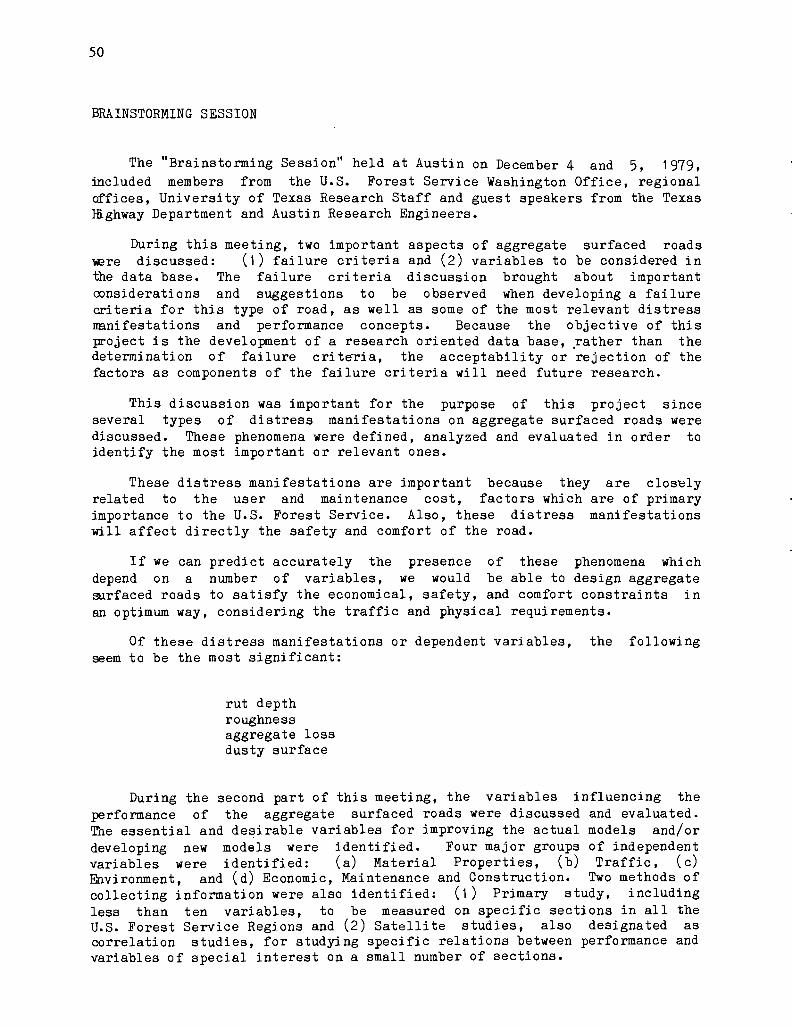
50
BRAINSTORMING SESSION
The "Brainstorming Session" held at Austin on December 4 and 5, 1979, included members from the U.S. Forest Service Washington Office, regional offices, University of Texas Research Staff and guest speakers from the Texas Highway Department and Austin Research Engineers.
During this meeting, two important aspects of aggregate surfaced roads ~re discussed: (1) failure criteria and (2) variables to be considered in the data base. The failure criteria discussion brought about important considerations and suggestions to be observed when developing a failure criteria for this type of road, as well as some of the most relevant distress manifestations and performance concepts. Because the objective of this project is the development of a research oriented data base, ,rather than the determination of failure crite~ia, the acceptability or rejection of the factors as components of the failure criteria will need future research.
This discussion was important for the purpose of this project since several types of distress manifestations on aggregate surfaced roads were discussed. These phenomena were defined, analyzed and evaluated in order to identify the most important or relevant ones.
These distress manifestations are important because they are closBly related to the user and maintenance cost, factors which are of primary importance to the U.S. Forest Service. Also, these distress manifestations will affect directly the safety and comfort of the road.
If we can predict accurately the presence of these phenomena which depend on a number of variables, we would be able to design aggregate surfaced roads to satisfy the economical, safety, and comfort constraints in an optimum way, considering the traffic and physical requirements.
Of these distress manifestations or dependent variables, the following seem to be the most significant:
rut depth roughness aggregate loss dusty surface
During the second part of this meeting, the variables influencing the performance of the aggregate surfaced roads were discussed and evaluated. The essential and desirable variables for improving the actual models and/or developing new models were identified. Four major groups of independent variables were identified: (a) Material Properties, (b) Traffic, (c) Environment, and (d) Economic, Maintenance and Construction. Two methods of collecting information were also identified: (1) Primary study, including less than ten variables, to be measured on specific sections in all the U.S. Forest Service Regions and (2) Satellite studies, also designated as correlation studies, for studying specific relations between performance and variables of special interest on a small number of sections.

51
A summary of this "brainstorming session" was completed, based on notes and tape recordings, and is provided in Appendix C.
A list of the variables to be collected is presented in Table 3.1. This table is divided into two parts, primary and satellite study, according to the type of the study where the information would be collected. Based on the type of variable, Table 3.1 is also divided into two groups: dependent and independent variables. The independent variables are classified in four groups, as described above.
SENSITIVITY ANALYSIS OF THE PDMS COMPUTER PROGRAM
During Phase III (Implementation of a Pavement Design and Management ~stem for Forest Service Roads), a sensitivity analysis of the PDMS computer program was performed. The basic concept for the sensitivity analysis, as stated in the Final Report of Phase III, is to evaluate the effect of changing the magnitude of a variable on the total project cost and rehabilitation strategy. In this way, the significant effects of different input variables could be compared.
The number of input variables for the case of aggregate surfaced roads was 47. The results of this sensitivity analysis showed that there were 24 variables significantly affecting the total cost. Of those 24, there were 16 Showing the largest effect. The results of the sensitivity analysis are presented in Table 3.2. According to the previous classification, these variables should be classified as independent variables.
Another important part of the sensitivity analysis was the study of the failure models (Rut Depth, Aggregate Loss, and AASHTO) to ascertain the ones controlling the pavement design for particular characteristics.
The Final Report from Phase III showed the Aggregate Loss Model controlled almost 40 percent of the most significant variables. The Rutting Model controlled only when the traffic characteristics (ranked number one in the sensitivity analysis results) were being considered. The AASHTO model, in general, controlled 60 percent of the most significant variables and also variables having small effect.
The sensitivity analysis indicates which variables are most important, and, therefore, indicates on which variables to concentrate resources to make accurate measurements for improving the models.
This sensitivity analysis was performed in May, 1978. Since this date, several modifications have been made to the PDMS program in such a way that a new sensitivity analysis will be required on the modified program dated May, 1980. We may postUlate the more significant variables should be the same because of the nature of the modifications performed.

52
TABLE 3.1. DATA BASE VARIABLES TO BE MEASURED AS RECOMMENDED DURING THE BRAINSTORMING SESSION
T Y P E o F STU D Y
PRIMARY SATELLITE
D DEPENDENT VARIABLES D 1. Rutting
2. Roughness
3. Aggregate Loss
4. Dusty Surface
INDEPENDENT VARIABLES
Material Properties
1. Structural Measurements: 1. Moisture Content
Number of Layers
Thickness of Layers
2. Quantification of Materials
Properties:
Strength
Atterberg limits
Gradation
2. Density
3. Resilient Modulus
4. Hardness (Soundness)
5. Aggregate Properties
Particle Shape
Degradation
6. Correlation between determina
tion of ~ in the field and in
the Laboratory
7. Seasonal variation of moisture
and density (as well as the
other variables)
8. Stability of Surfacing
9. Correlation between strength
testing methods
10. Deflections
(Continued)

53
TABLE 3.1. (CONTINUED)
Traffic
1. Number of Applications 1. Axle Loads
2. Distribution of the Traffic 2. Relation between aggregate 10ss
Traffic Speed
1. Precipitation
3. Relation of specific parameters
to Traffic (i.e., MMBE and
Traffic)
4. Measurement of monster vehicles
5. Tire pressure
6. HP
7. Configuration and types of axles
8. Affect of construction and
reconstruction vehicles
9. Weight ratio of vehicles
Environmental Variables
1. Depth of frost penetration
2. Temperature
3. Relation, if any, between lo
cation of the closer weather
station to the road
4. Relation, if any, between shaded
and non-shaded areas to moisture
5. Groundwater table
6. Snow dep th
7. Elevation
8. Wind
9. Freeze-thaw periods
(Continued)

54
TABLF ~.l. (CONTINUED)
Economic, Maintenance and Construction
1. Construction cost
2. Maintenance cost
3. Construction quality control
vs. performance
4. Maintenance records: number of
bladings
5. Affect of snow plowing on
aggregate loss
6. How to program seasonal closures
7. Quality of bladings vs. riding
quality
8. Dust vs. surfacing maintenance
9. Maintenance cost vs. performance
10. Water and rolling as maintenance
procedure
11. Energy cost of the maintenance
operation
12. Cost of tire wear
13. Cost of delays
14. Cost of accidents
15. Salvage value

55
TABLE 3.2. RESULTS OF THE SENSITIVITY ANALYSIS OF PDMS FOR AGGREGA TE SURFACED ROADS.
RELATIVE IN'" RANK VARIABLE CREASE IN COST*
.1 Traffic 1.53
2 Material cost, layer coefficient of 1.53 top layer
3 Aggregate surface loss 1.25
4 Soil support value of the subgrade 1.21
5 Salvage value of the top layer 1.16
6 Minimum thickness of an individual 1.10 rehabilitation
7 Grading cost 1.09
8 Regional factor 1.07
9 Material cost; layer coefficient and soil support of 2nd layer 1.07
10 Swelling clay parameter 1. 06
11 Interest rate 1.06
12 Minimum length of the performance per- 1.06 iod
13 Slope of the base 1.05
14 Accumulated maximum thickness of all 1.05 rehabilitation
15 Time between gradings 1.05
16 Annual routine maintenance cost 1.03
17 Terminal serviceability index 1.02
18 Average Approach speed to rehabilita- 1.01 tion
19 PSI and SI after an overlay 1.01
20 Non-deterioration parameter 1.01
21-47 Other variables 1.00
CONTROLLING FAILURE MODEL
R
L
A
L
A
A
A
L
L
L
A
L
A
A
A
A
A
A
A
A
A
*Increase in overall cost per mile using the highest value of the variable and compared with the overall cost when using an average value of this variable.
A = AASHTO Model L = Aggregate Loss 110del R = Rut Depth Model

56
C. T. COGHLAN QUESTIONNAIRE FOR AGGREGATE SURFACED ROADS
This questionnaire was sent to all regions of the U.S. Forest Service in July, 1979. Basically, two different questions were presented in this questi onnai re:
(1) How significant is a given factor to aggregate surfaced roads pavement design? and
(2) What are the most significant expressions of failure?
In answering the first included, as follows: Essential.
question, five possible rated answers were = None, 2 = Low, 3 = Moderate, 4 = High, and 5 =
A total of 111 factors were divided into five major groups as follows:
(1) Subgrade properties (SP), 24 factors
(2) Aggregate properties (AP), 55 factors
(3) Traffic (T), 9 factors
(4) Environment (E), 11 factors
(5) Management (M), 12 factors
This questionnaire took into account the qualifications of the engineers WlO replied by using an appropriate ranking system varying from 1 (Never designed a pavement and don't much care about it) to 5 (already have this all worked out and have all the answers).
The results from this survey showed that the most important factor concerning the design of aggregate surfaced roads is the "effect of moisture on subgrade strength," with a rank of 4.7. The least important factor is "field moisture equivalent related to lateral stability of aggregates," with a rank of 2.5 (Ref 18). A list of the 30 most important factors (ranked from 4.7 to 4.00) is presented in Table 3.3. As may be seen from Table 3.3, many factors are closely related to each other.
It may also be noted that many of those factors are not easy to measure because of their nature and large variability. The majority of these factors could be classified, according to the differentiation done in the part of the "Brainstorming Session," as independent variables. This means that these factors would interact with some other factors producing a particular condition on the pavement. This result or pavement condition would be one or a combination of the previously defined Dependent Variables, which are the factors realized by the road users. It is more practical and economical to measure these dependent variables than to measure the totality of the listed
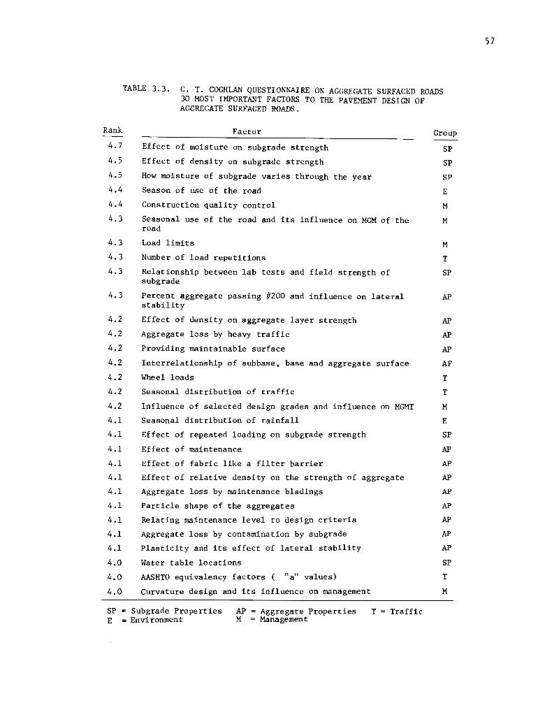
TABLE 3.3. C. T. COGHLAN QUESTIONNAIRE ON AGGREGATE SURFACED ROADS 30 MOST IMPORTANT FACTORS TO THE PAVEMENT DESIGN OF AGGREGATE SURFACED ROADS.
Rank
4.7
4.5
4.5
4.4
4.4
4.3
4.3
4.3
4.3
4.3
4.2
4.2
4.2
4.2
4.2
4.2
4.2
4.1
4.1
4.1
4.1
4.1
4.1
4.1
4.1
4.1
4.1
4.0
4.0
4.0
Factor
Effect of moisture on sub grade strength
Effect of density on subgrade strength
How moisture of subgrade varies through the year
Season of use of the road
Construction quality control
Seasonal use of the road and its influence on MGM of the road
Load limits
Number of load repetitions
Relationship between lab tests and field strength of subgrade
Percent aggregate passing #200 and influence on lateral stability
Effect of density on aggregate layer strength
Aggregate loss by-heavy traffic
Providing maintainable surface
Interrelationship of subbase, base and aggregate surface
Wheel loads
Seasonal distribution of traffic
Influence of selected design grades and influence on MGMT
Seasonal distribution of rainfall
Effect of repeated loading on subgrade strength
Effect of maintenance
Effect of fabric like a filter barrier
Effect of relative density on the strength of aggregate
Aggregate loss by maintenance bladings
Particle shape of the aggregates
Relating maintenance level to design criteria
Aggregate loss by contamination by sub grade
Plasticity and its effect of lateral stability
Water table locations
AASHTO equivalency factors "a" values)
Curvature design and its influence on management
SP Subgrade Properties E = Environment
AP = Aggregate Properties M Management
T l'raffic
Group
SP
SP
SP
E
M
M
M
T
SP
AP
AP
AP
AF
T
T
M
E
SP
AP
AP
AP
AP
AP
AP
AP
AP
SP
T
M
57

58
factors. Besides this, the measurements of these factors by themselves does not tell much. If we do not refer to them in some way, to pavement distress or performance, the measurements are less meaningful.
The presence of some factors in the list confirms the importance of variables, such as traffic variables (load applications, wheel loads, seasonal distribution, equivalence factors) and aggregate loss. It is also important to note those factors characterizing the materials, such as gradation, particle shape, plasticity, subgrade, and aggregate layers. The effect of density, which is directly related to construction quality control, should apparently play a very important role in the aggregate surfaced roads design. Many of these factors could be investigated in the "Satellite studies. "
A summary of the ranking of these factors is presented in Table 3.4, Where the percentages refer to the number of factors of each group (SP, AP, T, E, M) in 4 levels of importance. From this table we may notice the significance of the traffic variables, leading the first level of importance. It may be noticed that the groups: subgrade properties (SP), aggregate properties (AP), and traffic (T) have the same percentage of factors at the second level of importance. This analysis may give an indication of the group of variables deserving more attention. It is also important to realize that at this second level of importance the Management group has included 84 percent of its factor. From Table 3.3 it may be seen that the management factors, such as "construction quality control," "seasonal use of the road and its influence on management of the of the road," "load limi ts," etc., depend upon decisions that should be made based on knowledge of pavement parameters or models, which are not really available yet and that are the latest purpose of the Data Base.
According to this analysis, the importance of some variables has been quantified and corroborated, as in the case of aggregate loss, traffic, and many others that should be included in satellite studies. These results agree with the results from the two sources previously revised.
THE KENYA STUDY
The Kenya Study was conducted by the Transport and Research Laboratory (TRRL) and sponsored by the International Bank for Reconstruction and Development in two parts:
(1) Collection of information on the operating cost of vehicles relative to the road, geometrics, the surface characteristics and the environment.
(2) The study of the characterisitcs of the roads themselves and their relationships to the traffic carried, the environment, the original design and construction standards, and the different maintenance policies.

59
TABLE 3.4. RANGES OF IMPORTANCE TO THE PAVEMENT DESIGN OF AGGREGATE SURFACED ROADS OF THE FIVE GROUPS OF VARIABLES CONSIDER-ED IN THE "C. T. COGHLAN QUESTIONNAIRE"
Range of ImEortance Percentage of Factors in the Gro~
SP AP T E M
4.7 4.0 24% 25% 44% 18% 42%
4.0 3.5 51% 50% 33% 27% 42%
3.5 3.0 15% 15% 12% 55% 16%
3.0 2.5 10% 10% 11%
Total 100% 100% 100% 100% 100%
SP = Sub grade properties
AP = Aggregate prop~rties
T = Traffic
E = Enviornment
M = Management

60
Relationships between the variables computerized models were developed.
involved were derived and
The parameters that describe the condition of the road and are affected b,y the traffic and environment were measured. These performance parameters dealt with the unpaved roads:
(1) Surface roughness
(2) Rut depth
(3) Surface looseness
(4) Gravel loss
In the Kenya Study the following variables were selected for monitoring to explain the variation of these performance parameters:
(1) Rainfall (2 levels: low and high)
(2) Vertical geometry (3 levels: flat, intermediate and steep).
(3) Horizontal geometry (3 levels: low, medium, and high).
(4) Surface type (4 types: lateral, quartzitic, volcanic, and coral gravels).
(5) In addition, each gravel road section was duplicated or triplicated so that the effect of different levels of maintenance could be studied. Three levels were applied: normal maintenance (section graded each 6,000 vehicles), intermediate (section graded each 12,000 vehicles), and nil maintenance.
The unpaved road matrix is shown in Table 3.5.
Additional measurements were carried out on density, PI, and gradation); and on traffic factors, axle loads, traffic volumes).
material properties (CBR, measurements (equivalence
Each test section was one kilometer long with sections of similar characteristics extending for a half a kilometer on either side to act as a run-in. The test sections were concentrated in the southern region of the country, scattered in an area of approximately 170,000 km sq which represents 29 percent of the total area of the country. A total of 95 sections were used, 38 of them gravel sections, 8 earth surface, and 49 paved sections. The field work was conducted for 4 years in the first half of the 70's and some of the particular results and models are presented in Reference 20.

TABLE 3.5. CLASSIFICATION OF UNPAVED ROAD TEST SECTIONS IN TIlE KENYA STUDY
Road Low Rainfall High Rainfall Geometry <]OOOmm/year >lOOOmm/year
:s: Flat Inter- Steep Flat Inter- Steep <1.5% mediate ~3.5'-J mediate
~1.5%
Horizontal <3.5%
G28(I) G26(N) G33(N) G5 (I) G12(N) G29(Z) G3l(I) G35 (1) G7(N) G13(I)
Low «30° /kmJ G22(N) G32(Z) G36 (Z) E2(N)** G4l(N) G2l(N) G24(N)
Gravel Sections
(G) Medium(~300/km)G30 GlO(Z) (N) G34(N) G20(N) Gl(I) G6(N) «900/km}G42 G38(I) G25 (I) G2(N) Gll(N)
I (z) G 3(1)
High(~90° /km) G40(N) G16(N) G23(N) G17(I) G18(I) - G19(Z) El(N)
Low G27(N)* - - - E3(I) E4(Z)
Earth G37(I)* G15(1)* Sections Medium G39(N)* - - - -
(E)
High - - G14(N)* - - -
Note: (N) Normal maintenance level (I) Intermediate maintenance level (Z) Nil maintenance level * These sections were originally gravel sections but
were reclassified because the particle size distribution was poor.
** This section was originally an earth section but was reclassified as a gravel.
Gl-G19 Lateritic gravel G20-G25 Volcanic gravel G26-G38 Quartzitic gravel G39-G42 Coral gravel
61
I

62
BRAZIL STUDY (RESEARCH ON THE INTERRELATIONSHIP OF HIGHWAY COST)
The purpose of this study is to develop mathematical models for highway Planning and was sponsored by the government of Brazil, through the Empresa Brasileira de Planejaimento de Transportes (GEIPOT), the United Nations Development Program (UNDP) and the International Bank for Reconstruction and Development (IBRD). Basically, this study defines cost models which relate construction, maintenance and user cost for both paved and unpaved roads. lJhree major activities are identified in the Brazil Study:
(1) Road user cost surveys to determine the operating cost.
(2) Experiments to relate speed and fuel consumption.
(3) Pavement performance and maintenance experiments.
Of these three activities, the last one is the most interesting for our purpose of developing a data base for the PDMS program.
The parameters selected in this study to be monitored represent, in one or another way, pavement distress or define pavement performance. The selection of these parameters was, in the case of the unpaved roads (aggregate surfaced roads and earth surface), based on the results of previous research on pavement performance, with major input from the Kenya study. The selected parameters or dependent variables were:
(1) Roughness
(2) Gravel loss
(3 ) Looseness of gravel
(4) Rut depth
These dependent variables were monitored in the main study, considering the following five major factors:
(1) Type of surface material (three levels for aggregate surfaced roads)
(2) Traffic (ADT, two levels:high and low)
(3) Vertical geometry (high and low)
(4) Horizontal geometry (high and low)
(5) Maintenance (no maintenance, and every three months)

63
Also, a number of covariables such as percentage, heavy vehicles, total weight passing over the section per day, average daily distribution of the different vehicle types, passenger-car units, cumulative traffic since the last blading, number of days since the last blading, wet or dry season identification, and some material properties were considered. These covariables were monitored in the satellite studies. Some indicators of the applicability and limitations of this study may be inferred from the following paragraphs.
The test sections were widely scattered over central Brazil in an area of approximately 650,000 km sq. This area represents 8 percent of the total area of Brazil and 60 percent of of the road network of the country, which is around 1.5 million km sq (from Table 1.1).
In the main study a total of 113 sections were studied, divided into 65 paved sections and 48 unpaved sections (aggregate surfaced roads and unsurfaced roads). Of the 48 unpaved test section, 8 were replicates. The sampling matrix for the unpaved road experiment is shown in Table 3.6. Also, a set of star* pOints was selected to investigate nonlinear relationships in the regression analysis. Those sections possessing characteristics fulfilling the factor combinations for the star points are shown in Table 3.7. The typical test section was 720 meters long, divided into two subsections 320 meters long each and separated by an 80 meter long transition. A different maintenance level was provided each of the subsections as stated before. For comparison purposes and in order to get an idea of the resources involved in any study of this type and magnitude, it should be enough to mention that the Brazil project started in the middle of 1975 and the information collection phase ended in November 1979. Actually, the information is being analyzed in Brazil. The project cost, as stated in Ref 29, was over $13 million, with $750,000 being spent on instrumentation and equipment. A staff of over 165 was assembled including engineers, economists, technicians, administrators, clerks, and other support personnel.
RECOMMENDED STUDY VARIABLES
From these previous experiences, the following recommendations are made:
(1) Due to the large amount of variables affecting the pavement condition and due to the significance of these variables, it is recommended to divide the experiment into two types of studies: (a) the primary study, which would have national coverage and would include the measurement of the most important variables, and (b)
*The star point concept is used in the design of experiments methodology to cover intermediate and smaller and larger values of the variables to be monitored when compared to the selected limiting values.

TABL
E 3
.6.
UNPA
VED
ROAD
EX
PERI
MEN
TAL
DES
IGN
SA
MPL
ING
M
ATR
IX
IN
THE
BR
AZI
L ST
UD
Y
Tra
ffic
(A
DT)
Roa
d G
eom
etry
S
urf
acin
g M
ater
ial
Late
rite
Q
uart
zit
e
Wit
ho
ut
Su
rfac
ing
Ho
rizo
nta
l V
ert
ical
< 1
00
>
350
<
100
>
350
<
100
>
350
203
312
213
315
217
Cur
ve
~ 6%
20
9 21
5
R<
250
m
R<
250
m
. o
-1~
%
204
252
263
264
218
300
>
6 %
20
6 25
3 30
7 25
5 20
5 26
2 26
1 21
6
Tan
gent
o -
1~
%
202
251
259
254
201
313
302
304
The
nu
mbe
rs in
eac
h c
ell
refe
r to
th
e se
cti
on
num
ber.
i
"" .j:--

TABL
E 3
.7.
UNPA
VED
ROAD
ST
AR
POIN
T SA
MPL
ING
MA
TRIX
IN
TH
E B
RA
ZIL
STUD
Y
Lev
els
of
Tra
ffic
, V
ert
ical
Geo
met
ry a
nd H
ori
zon
tal
Geo
met
ry
Typ
e o
f T
r=*
Tr=
* T
r=*
Tr=
* T
r=*
Tr=
l T
r=2
Su
rfac
ing
V
G=*
V
G=*
V
G=*
V
G=l
V
G=2
V
G=*
V
G=*
HG
=*
HG
=l
HG
=2
HG
=*
HG
=*
HG
=*
HG
=*
Late
rite
21
4 31
0 25
6 21
1 31
1 21
2
Qu
artz
ite
309
303
258
301
257
308
305
Wit
hout
20
8 31
4 30
6 20
7 26
0 21
0 S
urf
acin
g
The
num
bers
in
eac
h cell
refe
r to
th
e se
ctio
n n
umbe
r.
Tr=
l if
ADT
<
100
vpd
T
r=*
if 1
50
< A
DT
< 3
00
Tr=
2 if
350
<
ADT
V
G=l
if
o <
Gra
de
< 1
.5%
V
G=*
if
3 <
Gra
de
<
5%
VG
=2 if
6
< G
rade
H
G=l
if
tan
gen
t H
G=*
if
250
<
Rad
ius<
45
0 m
H
G=2
if
250
~
Rad
ius
0'\
1.1
1

66
the satellite studies which would be performed in particular selected locations and would include the study of the pavement condition as affected by variables of secondary importance.
(2) There will be some dependent variables or pavement performance variables which will reflect in one or another way the failure of the pavement. These variables are the result of the interaction of a great number of factors which are called independent variables.
From the "Brainstorming Session," the Kenya study and from Brazil study the most important dependent variables roughness, aggregate loss, rutting, and loose material. variables should be measured in the Primary Study.
the are:
These
(4) The following independent variables are considered the most significant based on the five considered sources of information and are recommended for Primary Study.
a. Number of layers b. Layer thickness c. Strength and type of material d. Atterberg units e. Gradation f. Traffic, number of applications g. Distribution of the traffic (passenger cars,
pickups, trucks) h. Density and moisture measurements i. Maintenance level j. Environmental factors (Precipitation and
temperature index)
(5) From the Brainstorming Session, the PDMS sensitivity analysis, and the C.T. Coughlan Questionnaire, other independent variables deserving special consideration and requ1r1ng more extensive research were defined. These variables should be studied in the "Satellite Studies."
(6) The Brazil Study showed that data collection experiments with national coverage and scattered in a wide area may be performed successfuly if the appropriate planning, organization and coordination are properly provided.
In the following two chapters a review of the data collection procedures for these variables is presented.

CHAPTER 4. REVIEW AND SELECTION OF THE METHODS TO MEASURE DEPENDENT VARIABLES
In the previous chapter the variables involved in the pavement performance of aggregate surfaced roads were classified as dependent and independent variables. It was concluded that the dependent variables would be monitored in the Primary study. After reviewing major sources of information, four dependent variables were identified, namely: rut depth, roughness, aggregate loss, and looseness of materials.
Chapter 4 describes and evaluates the methods most measure each of these dependent variables. General selecting a methodology are also provided in this chapter. is placed on previous experience using these methods.
RUT DEPTH MEASUREMENTS
commonly used to recommendations in
Special emphasiS
Rutting is considered to be a major distress manifestation in any type of pavement. During the "brainstorming session" with the U.S: Forest Service Advisory Committee, it was concluded that rut depth was a relevant factor in the performance of aggregate surfaced roads for several reasons. It may determine the minimum layer thickness required in providing the adequate layer strength, in such a way that an underestimation of this distress manifestation may lead to a complete deterioration of the road. Associated with the presence of rutting are the surface channels, which would carry or contain water, possibly eroding the road surface and reducing its load carrying capacity.
The great significance of the rutting model in PDMS, and the necessity to validate this model has been confirmed by the Sensitivity Analysis of PDMS.
Two devices may be used to measure rut depth: the AASHTO type rut depth gauge and the transverse profile gauge. Both devices are described and evaluated here. Special attention is given to the description of the AASHTO type rut depth gauge as used in the Brazil study. A system to classify the ruts and obtain a better knowledge of this distress manifestation is included at the end of this section.
AASHTO Type Rut Depth Gauge
This device, developed during the AASHO Road Test, has been widely used around the world for measuring rut depth, because of its simplicity in operation and in transportation, as well as of the low acquisition cost.
67

68
It consists of a triangular aluminium frame with a graduated aluminium or steel bar which slides vertically through the center of the frame. The sliding bar is provided with a scale. The scale zero is in coincidence with the top edge of the frame when the instrument is standing on a flat surface; hence, this is the datum point against which depth measurement readings are taken.
During the aggregate surfaced roads rut depth measurements in Brazil, this device was slightly modified by providing the frame with a bottom cross bar to eliminate the influence of localized depressions on the measurements, as shown in Fig 4.1. To permit the instrument to be used on paved roads, the bottom cross member was removed. A smaller version was re~uired in Brazil in order to be transported in small vehicles. This was made in the same way, as the gauge from Fig 4.1, with the exception that its height was reduced by 20 cm (8 in). In the Brazil Study, the material used to manufacture the vertical sliding bar was changed to steel in later instruments, since the aluminium bar had a tendency to stick.
The operating method for gravel roads, as described in Ref 21, consists of laying the instrument across the rut to be measured with the sliding bar above the lowest point in the rut. This establishes the road surface level. The graduated bar is then allowed to slide down until its lower end rests in the bottom of the rut, but is not pressed down deeply into the material below the bottom of the rut. In taking rut depth readings, it is important to have the recording eye at the same level each time to obtain accurate readings.
In Brazil, rut depth measurements were obtained every two weeks. On the sections receiving high level maintenance, one grading every two weeks, measurements were taken five times within the two week interval.
The measurements were taken at five equally spaced positions within each 300 meter lon~ subsection. The first and last positions were taken to coincide with the two extremes of the subsection. The rut depth measurements were taken by the roughness measurements crew, hence the equal spacing was established using the electronic distance measuring instrument (DMI) mounted on the vehicle, as explained later in the Maysmeter description.
Because of the nature of the aggregate roads, the ruts were defined as those positions on the road where the majority of the vehicles travel. These areas are easily identified by the absence of loose material. When more than four wheel tracks existed, only those tracks were measured and the other measurement positions were left blank on the field form shown in Fig 4.2.
The rut depth measurement crew consisted of two men, one handling the rut depth gauge and the other recording the readings. In order to take measurements rapidly, it is recommended to have permanent concrete markers in the sections.
Transverse Profile Gauge
The transverse profile gauge or transverse profilograph is another device that has been widely used for rut depth measurements. A 2 meter (6

69
0-30em Steel Scale
/Datum Point
E ()
rt') rt')
E ()
If)
N
E 60em ()
E If) ()
", If) . CD If)
122 em
Fig 4.1. AASHTO rut depth gauge as used in the Brazil study.

MT
-GE
JPO
T
( T£
CN
tCO
S
]
PIC
R -E
STU
DO
S
DO
S P
AV
IME
NTO
S
FLE
CH
A D
AS
TR
ILH
AS
E
CO
RR
UG
ACO
ES
Dls
r ~
'01(,"
" D
ATA
IN
,1!(
•
C
RO
OO
\IIA
~~;
.t:: S
(N,
TR
l.HA
~ •
N ~
10 D
M M
Al.
Im
l ,
8 :I
EXT.
ESC
I
8 :s
INT,
ESO
2
e :s
INT.
DR
,
81--1
EX
TOIR
4
813
XU
'SO
I
8 :s
INT.
ESO
2
e h
WTD
lR.
1
e 3
EX
TO
l" 4
--
83
£X
1£5O
I
8 3
ME
SO
2
al ~
tNT.
OIR
)
8 I.
£X
T.D
IR <
1
~-~~r-'1~~~~4-~-~~
er~
(XT
£9>
I
al~
ME
SO
2
1-
a 3
ffl,O
IR.
:I
13
O
O.O
IR
4
"'.li."'O"~J41'''7,·"rx21
iu
LEIT
UR
A
DA
P
RO
f';N
OIC
A(j
£
iliA
SE
tAO
TR
AN
SV
ER
SA
L ,..
~ Im
ml
CO
RR
UG
AC
OE
S
I~
2~
l~
." S"
6~
7~
s·
9~
10
· Ir-I ....
. ~
JO[c
>oi
Itn
t
SEt,(
Card
Id
en
tifi
cati
on
N
um
ber
, 8
3
Co
l 1
-2
Co
l 3
-7
Co
l 8
-10
C
ol
11
-16
.
Ro
ad N
utr
ber
1 C
OM
Secti
On
N
utr
ber
Date
Co
l 1
7-1
9
Dis
tan
ce b
etw
een
C
ross
-Secti
on
s
Co
l 2
0-2
1
Dir
ecti
on
, SC
o
u C
S
Co
l 2
2
Car
d N
o 1
-L
eft
Ex
tern
al
Wh
eelp
ath
Cat
:d N
o 2
-L
eft
In
tern
al
Wh
eelp
ath
Car
d N
o 3
-R
igh
t In
tern
al
Wh
eelp
ath
ca.r
d. N
o 4
-R
igh
t E
xte
rnal
Wh
eelp
ath
S£M
Co
l 2
3-5
2
Ru
t D
epth
at
Cro
ss-S
ecti
on
Nu
mb
er
(mm
) in
q
rou
ps·o
f 3
colu
mn
s
Co
l ·5~
Co
l 5
4-5
6
ICo
l 5
7-5
9
L.
Are
th
ere
co
rru
qati
on
s
Yes
(S)
or
No
(N)
"Dep
th o
f co
rru
qati
on
s
(nun
) E
xte
nt
of
co
rru
qati
on
s
(m)
Sp
acin
q o
f co
rru
qati
on
s
(em
) A
vera
qe w
idth
o
f co
rru
qati
on
s
I
(!!o
"IlC
O
L.&
II',
..
Fig
4
.2.
Rut
d
epth
mea
sure
men
ts fi
eld
fo
rm
as
use
d in
th
e B
razil
stu
dy
.
--.J
o
71
ft) transverse profilograph was used during the Kenya study (Ref 19) and a 3.96 meter (13 ft) device was used in Oklahoma as reported by Oteng-Seifah and Manke eta al., Ref 22. The first study made measurements on aggregate roads and the latter one on asphalt concrete pavements.
The device reported in Reference 22, provides a continuous profile tracing of the pavement surface, thus, the shape of the pavement surface adjacent to the wheel path depressions is ascertained and the rut depth is measured to the nearest 0.025 cm. (0.01 in). The transverse profilograph consi~ts basically of: (1) a supported guide rail, (2) a trolley system, and ,3) "X - y" recorder. The profilometer is made from two magnesium alloy carpenter's framing levels.
The rail is supported at the center pOint and the ends with adjustable height supports and is oriented to span a traffic lane perpendicular to the centerline of the roadway. The two end supports are adjusted to set the rail at a given height above the pavement surface at these points; the center support is adjusted to remove any midspan deflection. Thus, the rail becomes a planar surface and serves as a guide for the trolley system and as the datum for the measurements.
The trolley system consists of an aluminium suspension plate with four nylon rail-track wheels machined to fit the top and bottom flanges of the rail. A rubber-rimmed actuating wheel, made of teflon, is attached to a short pivot arm hinged to the bottom of the suspension plate. The pivot arm also supports a helical potentiometer, whose shaft is connected to the axle of the actuating wheel, and a bracket connection for one end of a linear potentiometer. The other end of this linear potentiometer is attached to the suspension plate.
The actuating wheel contacts and rolls along the pavement surface as the trolley system traverses the guide rail. The helical potentiometer scales the horizontal displacement, and the linear potentiometer scales the vertical displacement of the actuating wheel. These displacements are recorded as a continuous transverse profile trace of the pavement surface by an X-y recorder.
A similar device is commercially manufactured by Rainhart Co., Austin, Texas, and is illustrated in Fig 4.3. The shipping weight is around 63 kg (140 lb), and the acquisition cost is about $1,000.
This device requires a two-man operational crew. By using this device, the entire transverse profile of the road may be obtained, but the device may provide too much information for rut depth measurement purposes and requires excessive office work to be interpreted and codified. However, if the leveled transverse profilograph is referred to a permanent benchmark, the information may also be used for aggregate loss measurements. This may be appropriate if these two pavement distress manifestations are measured with the same periodicity and at the same locations (which in fact, may not always be convenient). On the other hand, only one crew and one simple and relatively inexpensive device is being used. The disadvantage is the extra man-hours required for codifying and interpreting the data. A cost analysis of this procedure is required in order to make a proper decision.

a)
Tro
lley
sy
stem
b)
Fro
nt
view
Fig
4.3
. T
ran
sver
se p
rofi
log
rap
h a
s m
anu
fact
ure
d b
y R
ain
har
t C
ompa
ny,
Au
stin
, T
exas
.
'" I'-'

73
In Kenya, the rut depth measurements were made in all the wheel tracks present in the section, and the mean value of these measurements used as the final rut depth value for the section. The measurements were taken at each end of the one-thousand meter-long (3,280 ft) section and at one end of the 100 meter (328 ft) sections used for recording gravel loss.
A pneumatically operated transverse profilometer was used during the AASHO Road Test \Ref 23), for measuring the transverse profile. The information was automatically recorded by an electronic device which is shown in Fig 4.4.
Complementary Rut Depth Measurements
The devices previously described provide the magnitude the problem. Because there are different types of rutting, descriptive rutting measurements be made in order to better phenomenon.
or severity of it is recommended understand this
These measurements would provide the classification and or1g1n of the rutting, which in aggregate surfaced roads may be attributed to an~ of the following four reasons: (1) densification after construction, (2) shear failure of the surface layer, (3) shear failure of the sub~rade material, and (4) redistribution of the gravel by the traffic action. These rutting types will have different physical manifestations as shown in Fig 4.5.
The first step in the study of rutting, besides the measurement of the rut depth (RD in Fig 4.5), would be the external identification of the rut. Two external shapes may be recognized, as illustrated in Figs 4.5.a and 4.5.c, and are designated Type "V" and Type "M", respectively.
Once the external shape has been identified, the next step would be the differentiation of the rut Type "V" in two groups: (1) due to densification and/or redistribution. of the surface material, and (2) due to shear failure of the subgrade. In achieving this, it would be necessary to dig trenches and study the layers profile, to determine if the failure is due to densification or redistribution of the surface material or to subgrade failure. This type of study was conducted during the AASHO Road Test (Ref 24), using trenches 0.98 meter (3 ft) wide along the cross sections. While the trenches were being made, precise levels were taken at 0.30 meter (1 foot) intervals laterally on top of each of the layers and at both faces of the trench. Additionally, cores for density determination were taken of the surfacing course, and in place density, CBR, and moisture content determination of the granular materials and embankment soil were made. These studies were performed in sections with serviceability indexes below the minimum acceptable.
Because of the more general nature of these studies, they should be made when rut depth reaches an excessive level, before a grading operation, or before a regravelling operation. In order to track the variations in rutting, it would be necessary to dig trenches before or after the situations previously mentioned. When the trench is dug, the material is disturbed even though the trench is filled with the same material, but this trench may not

74
Fig 4.4. Transverse profilometer as us.ed in the AASHO Road Test (Ref 23).

Aoore oate Surface
Suborade
Ca) Densification and/or redistribution of the gravel by the traffic action.
'0·' \) :' 0 ~'()',.o·. ",0', • ..; ,f1 '" .. ,. • ~. O . ..
" . 0 . '. '. ~ . · -(/' .. 0 " . t?,·O·. . o· .. '" ~ .. , '. I....... ..' -) . . " ',. 0 '. 0 . • .
~ (b) Sh,ear failure of the subgrade.
." .
Aogregate
Surface
Suborade
'0 . • (') 0' • • Aggregate :.; ~ : '. . , o· o •• ' . 0 Surface ,,0 • ." ., '.c::::> ","
.,.' I 0 ., C/ '.. . •
~iw~~ Suborade
(c) Shear failure of the surface layer.
Fig 4.5. Rutting physical manifestations and its causes.
7':'

76
be used again as a sampling trench. So, it would be necessary to design a section that allows for the necessary number of trenches. The trenches would be excavated in an alternate fashion. With this, a better knowledge of rutting may be obtained. These complementary rut depth measurements might be performed on a satellite study.
Selecting a Rut Depth Measuring Device
In measuring rut depth, the AASHTO Type Rut Depth Gauge seems to be a very practical, simple, and economical device. The Transverse Profile Gauge appears to be an accurate and more expensive method. Although, if it is also used for aggregate loss measurements, its potential increases in such a way that a decision should be made based on a cost analysis and probably after trying both methods during a pilot study. It is recommended to include, as a part of the rut depth measurements, the classification of the rutting type.
ROUGHNESS MEASUREMENTS
The roughness concept has received considerable attention in the last twenty years from many highway and airport agencies around the world. In the case of asphalt or Portland cement concrete, roughness is a determinant factor in defining the Present Serviceability Index (PSI) of the pavement, which is normally used as a failure criteria in these types of roads. The criteria involved in designing these roads consider that the roads are provided for, and by, the users, and they must provide a safe, smooth and comfortable ride. Because of the characteristics of the roads managed by the Forest Service, it may be said that the majority of these roads must provide a safe, acceptable, and economical ride. Thus, roughness may not be primarily associated to the serviceability concept and may be considered as a pavement distress manifestation, as an indicator that something is not performing properly in the pavement structure. The study of the roughness phenomenon in aggregate surfaced roads must bring, among other benefits, important improvements to the structural model included in PDMS and may provide the basis for unified maintenance criteria for the Forest Service roads.
In order to quantify the roughness of a road, many devices have been developed. In the following pages four of them are described with comments. The preselected devices are the BPR Roughometer, the Surface Dynamics Profilometer (SDP), the PCA Road Meter, and the Maysmeter. Of the Mays Meter, three versions have been considered. In the last part of this section, some recommendations in selecting a roughness measurement system are presented.·
The BPR Roughometer
As described by Haas and Hudson (Ref 10), the BPR Roughometer has been used by many agencies since 1920. It is a trailer-type device, as

77
illustr~ted in Fig 4.6, that simulates one wheel of a passenger car and is comprised of a mass, spring, and damper combination.
The roughness of the road is measured by the displacement of the wheel with respect to the mass. This displacement is recorded by an integrator coupled to an electronic counter. The counter is calibrated to record inches of vertical movement of the axle relative to the top of the suspension system. Accumulation of the displacement over a distance interval is called roughness index, computed in inches/mile. The operating speed is 20 mph, when towed by a light vehicle. The limitations are low operating speed, attenuation of wavelength in the ride frequency range, poor repeatability, and a requirement for constant calibration.
Surface ~namics Profilometer (SDP)
Originally known as the GMR Profilomete~, it was developed by the General Motors Corporation, in Warren, Michigan. K.J. Law Engineering in DetrOit, began manufacturing the SDP in 1966. The basic operational principle is based on the use of a series of accelerometers. The SDP is contained in a van and consists of two road-following wheels mounted on trailing arms beneath the vehicle, one in each wheel path, and it is held in contact with the road by a 300 lb. spring force. Relative motion between the vehicle and the wheel is measured by a potentiometer mounted on the vehicle body above the road-following wheels at a point where an accelerometer measures the acceleration of the vehicle itself, see Fig 4.7. The truck mass and truck suspension form a mechanical filter between the road and the accelerometer.
The signal from the accelerometer and the potentiometer are input into an analog computer carried in the vehicle. The acceleration signal is integrated twice and added to the potentiometer signal, then conditioned to obtain right or left true profile, see Fig 4.8.
Wavelengths longer than approximately 200 ft are attenuated toward zero in proportion to their amplitude. Thus, it may be said the device gives a good indication of true profile for wavelengths shorter than approximately 200 ft and produces a signal proportional to true profile for longer wavelengths.
The profile data obtained in analog form is amenable to power spectral density processing, but other parameters such as slope variance or roughness indices are difficult to obtain. Consequently, analog-to-digital and digital processing subsystems must also be developed or adapted to obtain increased flexibility.
The advantages of the SDP in comparison to other devices are: (1) determination of actual profiles, (2) capability of handlin~ large amounts of data by automated means, (3) high operation speed, (40-50 mph), and consequently, high production per day, (4) capability of detecting and analyzing longer wavelengths, (5) excellent repeatability, (6) capability of use for calibration of a car road meter, and (7) calibration is not required.

78
•
Integrator
Fig 4.6. Schematic of BPR roughometer and trailer (Ref 10).

ANALOG COMPUTATION
Ir--:--=---Cl-- ACCELEROMETER
w
Fig 4.7. Principle of the GMR profilometer (Ref 25).
79

80
Output Analog Trace of Pavement Elevation Profile (Paper or Magnetic Tope)
r---------~----r- - -- --..J.......r I I I I Double
~lnt.grQtion
I I I I I I I I I
Accelerome ter Inertial r--- Reference (Output t 29)
~---------------- ..
Linear Motion Transducer (Output t 4inches)
Fig 4.8. Schematic of GMR profilometer (Ref 26).

81
The disadvantages of the SDP are as follows: (1) high capital cost, (2) high operation cost, (3) n~ed for highly skilled personnel, (4) complexity of the system, and (5) high computation cost.
This device has been widely used in Texas, Michigan, and in the Brazil study as a calibration device for the Maysmeter. The primary characteristic of the SDP is the capability of measuring the true profile of the road.
The PCA Road Meter
The PCA Road Meter was developed in 1965 to afford a rapid method for measuring slope variance. This device uses a simple electromechanical device installed in a conventional passenger automobile which measures the number and magnitude of vertical deviations between the body of the automobile and the center of the rear axle.
It has been widely used by the Portland Cement Association. As described by M.P. Brokaw (Ref 27), this device consists of a flexible, braided steel strand connected to the top center of the rear axle housing in a vehicle. The steel strand extends vertically through the trunk compartment, and then through a small hole in the package deck just behind the rear seat, see Fig 4.9. At this pOint, the strand passes over a transverse-mounted pulley, and is restrained by a tension spring attached to a small post on the package deck at a point near the right side of the body shell. Thus, vertical movement between the rear axle housing and the package deck is translated to horizontal movement of the strand.
Midway between the pulley and the tension spring, a roller microswitch is attached to the metal strand. The switch is mounted in a rectangular formica plate that slides in transverse metal guides.
The microswitch roller impinges on a switch plate, constructed so transverse roller movements can be measured in 1/8 inch increments, either plus or minus from a reference standing position of the automobile. The switch plate, divided into twenty three 1/8 inch segments, is also mounted in transverse metal guides.
The transverse reference position of the switch under the roller to accommodate various static loads adjustment is made by a separate tension-spring control.
plate can be adjusted in the automobile. This attachment and vernier
Automotive electric power is inserted in the roller and switch plate system. Output is directed to visual indicators of road-car deviations, mounted in a console placed just above the automobile instrument panel. Electric counters are mounted on a separate chassis resting on the floor of the automobile.
Methods for reducing counter data have been given intensive study. Each counter accumulates the number of impulses equal to or greater than its segment number. A counter will also record a double-count for impulses that are greater than its segment number.

Anc
hor
Rol
ler
+ 12
V.
(DC
) /
Fle
xib
le
Ste
el S
tran
d
L _ _
F
ixe
d P
ulle
y _Ten.~~
_ ~:
m. _
---~--I
III!
II
rlll
;t:o
;f;1
I1I1
i 1
III
I-
:I
j i
Rolle
; Con
toct
o'";
--
--
,..."
.z.
Dev
iatio
n Sw
i tch
2
3 C
onto
cts
Fix
ed S
pool
on
d V
ern
ier
Ad
just
men
t R
ear
Pac
kage
Dec
k::::
:::"
Ele
ctri
c C
able
J'F
tt
~ o
f A
utom
obile
to
Con
trol
C
onso
le
,,
Sin
gle
Pol
e ~~ 0
0
12-P
osi
tio
n
,:
Sw
itch
-51
\.0 I
oJ
'0
0 !"
,
4.1
In
dic
a la
rs
• * ~ment to
C
ente
r R
ear
Ax
le H
ousi
ng
No
t to
S
ca
le
Fig
4.9
. D
iagr
am o
f m
ech
anic
al a
nd
ele
ctr
ical
featu
res
of
the
peA
ro
ad m
eter
(R
ef 2
7).
00
N

83
Several versions of the PCA Road Meter have been developed, one of thembeing the Wisconsin Road Meter, Fig. 4.10. This road meter is manufactured by Soil test Inc., Evanston, Ill. The acquisition cost of this version of the PCA Road Meter is around $ 1,745.00.
In order to check the reproducibility of results from the PCA Road Meter, several studies have been conducted. One performed by the Minnesota Department of Highways and reported by P.C. Hughes, Ref 28, checked the repeatability of the Road Meter under the same operating conditions. Running the Road Meter five times on seven sections of pavement, it was found that the Road Meter showed an excellent repeatability under the same operating conditions as shown in Table D.1, Appendix D.
Also, there was an investigation into what changes in operating yonditions would affect the results reached with the Road Meter as follows: \1) Type of tire had very little effect, (2) tire pressure had no significant effect in normal inflation range, (3) speed of ~he automobile had a significant effect, (4) load in the automobile must be stable and no passengers in back seats, (5) air temperature should be above fifteen degrees Fahrenheit, (6) wind velocity of 15 mph or greater had a detrimental effect and crosswinds had more effect, and (7) type of automobile.
A detailed description of the research performed on the effects of these factors is presented in Appendix D.
The advantages of using the PCA Road Meter for roughness measurements are as follow: (1) low initial investment, (2) high operation speed, (3) only one roughness reading for each section, data is reduced.
Among the disadvantages, it is important to mention the following: (1) constant calibration is required, \2) difficult installation, (3) the measurement system seems to be very susceptible to small variations (tension in the cable, properties of the spring, etc.), and consequently susceptible to errors, (4) the maximum roughness depth that can be measured with this device is 10/8 inches, a value that in aggregate surfaced roads must be very common and probably greater. This fact may be solved by making th~ scale greater, maybe twice the present size, and (5) high operating cost because of constant calibration.
Some of the agencies that have used the PCA Road Meter are the Minnesota Department of Highways, the Iowa State Highway Commission, the Wisconsin Division of Highways, and the British Columbia Department of Highways.
The Maysmeter
In this section three versions of the Maysmeter are described and evaluated, namely the Standard Maysmeter, the Brazil study Maysmeter, and the Texas SDHPT Maysmeter System. Important aspects of the Maysmeter measurements variability, as well as the most important advantages and disadvantages of the Maysmeter when compared to other roughness measuring devices, are presented in the last part of this section.

84
Fig 4.10. The Wisconsin road meter.

85
The Standard Maysmeter. The Maysmeter is a three major component device: (1) transmitter, (2) distance measurement system, and (3) output system, see Fig 4.11.
The transmitter is rigidly attached to the car's body immediately above the differential and consists of a case in which is mounted a film strip with blanket and open windows for the transmission of light from a 12-volt lamp. The film strip is formed into a circle and is driven in a circular motion by a wheel attached to it through a drive shaft. The wheel is mounted on the outside of the transmitter housing and is driven by a bow rod. The lower end of the rod is attached to the center of the rear axle of the vehicle, as illustrated in Fig 4.12. The rod extends up through the vehicle's floor through a hole and passes up and down in contact with the transmitter wheel. A steel flexible cable is wrapped one turn around the transmitter wheel and attached to each end of the bow rod. The transmitter is attached to the vehicle's floor just over the center of the rear axle.
As the vehicle body is displaced relative to the rear axle, the transmitter is made to transmit a series of electrical pulses, one for each tenth inch of displacement, to the summation unit.
The second major component is the distance measuring system, which is integrated in the form of an odometer of the push-button reset type and reads to 0.01 mile. The odometer is driven through a tee inserted in the speedometer cable; its readout numbers approximate the parent vehicle's odometer. It is mounted in such a way that it can be easily read and conveniently operated by both the driver and the operator.
The output from the standard Maysmeter is printed in a six inch wide "z" fold strip chart, displaying three synchronized traces:· distance, profile, and landmarks. Of these, the latter is optional. Fig 4.13 presents a Maysmeter in operation, and Fig 4.14 illustrates a typical 9utput. The distance measurement system traces automatically, zigs for 0.05 miles.' and zags for 0.05 mile6. recording the information generated by the odometer. The paper is fed in increments of 1/64 inch for each and every 0.10 inch of rear axle/body excursion, in such a way that a perfectly smooth pavement would not drive the chart, and a rough pavement would consume a great length of paper. Dividing the length of paper produced, measured in inches, by the distance travelled and by 64, the result would be the number of 0.10 inch displacements of the rear axle relative to the car's body. The profile trace follows the rear axle excursions in the same direction, and at half the magnitude displaying surface peculiarities. In this way, the maximum deviation that can be measured would be twelve inches.
The landmarks trace alternately zigs or zags at the touch of a push button to pinpoint the beginning or ending of a test section, bridge or overlay; the location of intersections and surface imperfections can also be fixed.
The ~tandard Maysmeter has been widely used in the United States and abroad. Some of the users are the Florida Department of Transportationt the Louisiana Department of Transportation; the Pennsylvania Department of Transportation; the Texas State Department of Highways and Public

86
Tronsmi tter
Odometer
----
Recorder
Fig 4.11. Stanrlard ~ meter three major components.

87
Fig 4.12. Mays meter transmitter unit (Ref 33).

88
Fig 4.13. Standard Mays meter in operation (Ref 33).

_C
HA
Iff F
ED B
Y R
EA
R A
XLE
EX
CU
RS
IOlfS
••••
••••
••••
••••
••••
••••
••••
••••
••••
••••
••••
••••
••••
••
DIS
TAN
CE
<odo
tnem
)
"=1
=
I i 'm~i
,-----+----c
---,:_~,
C-¥
i.W
I
1:3
• •
i '
""" I
. .:-:
-:-:
==
:--,
---
--,
.. __
. .
. ,_
-+
--'
__ -+
'
.,. ___ -
-=+=-
-,g
J !
J
f~·. ._J
.ic
eK
iiir ~.-
-~-: --.. :
' ~ ~ ......
..,.~----'-.
:....-...=..
:-=--=T: •.. ~-T
~~-:
t~L<
'--
. .':~~ ""e
.'OLE
.-~~~ ::
-;~+~:~.
'c·~~==T
--:s= "'
-" -
"-.
..
(~Ie 5
5mph
. thi
s o
etv
c ..
I
f'eSt
ru
n--
-;-
j'l~=--.
..; =~l-=-u-+=-L
-"J
. ~~.
-t
.-'--
hOJ
.. J -:....
. 'i
-fi
eld
"otn
U
t-.
::-.
-.
! -I
..
_ J!
!! f
11'1-
' I!.
..L
A
ll_
.;,..,..
__
. __
__
_ .
"".
--"~-->.
..:j
];"
....
,.:K
'-:;:
.. .u
. -
rJ
--_
._'_
r--r~
I!I
....
..""
fIr
_ _
,fo
l'---
-:·.:J··
!"-fl
:k::.
.
'"
-1:_
. : ..
. -i,
... r=
_ ...
. : ~A
NDMARK
S m
.
?-..
.. ...
.. !
=r
mon
uol u
op.,
',=~.
. ,-~ -' ....
.......... -.. -
.... =
..;;
.,I'
""--
'!
(.0
. ...n~""',
'("
UI
7 ...
. -'~
01
. to
f;J.
1:0<
1 r~(CI:.)t. e
M""
l\II
O n
, tA
t."
....
.. flO
....
fl.""
'IT
t.
.N'
Itnl"f
.. .tu
(.0
. A
US
TjN
. T
o.A
I
••••••••••••••••••••••••••••••••••••••••••••••••••••••
Fig
4.1
4.
Sta
nd
ard
May
s m
eter
ou
tpu
t.
00
\0

90
Transportation. study (Ref 20)
With some modifications, it has been used in the and in roughness measurements in Bolivia (Ref 29).
Brazil
The Brazil Study Maysmeter System. During the Brazil study two major modifications were done to the odometer and output systems of the Standard Maysmeter. The odometer unit was replaced by an electronic distance measuring instrument, DMI, to permit roughness measurements to be obtained over fixed distance intervals. The DMI sensor, manufactured by Nu-Metrics, Connellsville, Pa., is, as described in Ref 30, mounted near the vehicle's front wheel, which is equipped wi~h eight target magnets, Fig 4.15. As each magnet passes the sensor, it issues a pulse to the input signal conditioner circuit. The DMI measures the distance traveled by the vehicle by counting the revolutions of the vehicle's front wheel. The DMI is believed to be more accurate than the mechanical odometer system originally provided with the Maysmeter. The distance travelled is continuously displayed on the DMI front panel, and the electrical signal is routed to the 'summation unit.
In order to speed the data collection and data reduction process, the Standard Maysmeter chart recorder was replaced by a digital readout, especially designed and constructed, Fig 4.16. The unit sums road roughness data and displays it at either 0.050 miles (80 meter), or 0.20 miles (320 meters) , intervals.
This output system receives roughness related electrical pulses from the transmiter unit and divides the pulse count by two. The count is accumulated in a special counter, which is incremented by one each time the vehicle's body changes position relative to the rear axle by two tenths of an inch. Information related to the distance traveled is also received in the unit in the form of electrical pulses from the DMI. The unit sums these pulses in a special binary counter. When the proper count is reached, representing either 0.050 miles or 0.20 miles, the interval being selected by the operator, the accumulated roughness count is made to replace the count currently in the four digitals display unit, Fig 4.17. At the same time, the roughness counter is set to zero, ready to start summing the roughness of the next selected interval. The operator is alerted to copy the new count by an audible tone which sounds just as the new count replaces the old count.
The DMI and the summation unit are fixed together via a mounting bracket and fixed to the vehicle instrument panel in a uniquely constructed panel which allows mounting the units in the glove box or other suitable opening.
Seven Maysmeter units were used in this study, and were calibrated by means of a GM Surface Dynamics Profilometer. The output from these devices has units of length per length, but to avoid confusion with other roughness measurements, the unl~S were designated counts/km and the roughness index named quarter-car index (QI). The cost of this Maysmeter configuration is around $2,900.00.
The Texas SDHPT Maysmeter System. As reported by Goss, Hankins, and Hubbard et. a1., Ref 31, the Texas SDHPT implemented in 1976 a Maysmeter device mounted in a specially designed and constructed trailer, which is pulled by any light vehicle. This was done in order to minimize the variations in the Maysmeter output due to changes in the tire pressure, in

91
Targets
Fig 4.15. Targets disposition used by the Brazil version of the Mays meter.

~~ 0
~ O~ ~
0 rz>
I~~~~~I
KIL
OM
ETE
RS
M
ET
ER
S
~~ -
1= ]-1
-
I -,
1_' I
-C]
-
@
I _I
I
I I
~~ O
N
HO
LD
RE
SE
T CA
L.I;}
-
-II
III III
III II D
ISTA
NC
E
ME
AS
UR
EM
EN
T IN
ST
RU
ME
NT
['\.
/ e
PO
WE
R
LEN
GTH
11~1
) I
1-'
-I
:'
on
0 .0
5 I
I_I
1= _
I
@
®
-I
1-
off
.20
L
( "-
e - -
Fig
4
.16
. D
igit
al
read
ou
t u
sed
by
the
Bra
zil
vers
ion
of
the
May
s m
ete
r.
0 0
\0
~

... -------------------------- - - ----------II n n n
I I -I
r n III II II I I I I II Accumulative
I~_I -I ------1~n~Counter F=======~:db::db:~==~~~d:~==~====~11
n il
I-I I 1
I I I I
I-I -I
II II
I-I :: Alternat ino I-I -I I _ -I ;: Counter s
F=::::!::::::===:!6::!::=::::!:::::::!::::::::::::!==::::!:=::::!::::&~b::b=='==I .. ~ II Seoment
I I I_I
. 2 ~.O 5 ... -.. _i----------fl-&f-
ilLL--t;~=====:::;==~~:;:;:;~=;::~~;;:;;:=~I' I Lenoth Switch Cj) I "..Q ~ .Jl .JJ I 01 S~NC~ I~ MI LE':
.J..o&o~~. rn III I II ON HOLD RST BI-OI I CI =1 I] -I
1 0 0 0 0 1
Distance ~I-Measurino
Instrument
Fig 4.17. Electronic counter system used by the Texas SDHPT version of the Mays meter.
93

94
the vehicle weight, and in the vehicle's operating speed. The use of a trailer would stabilize the weight variables, since weight could be constant due t? fuel use, (no decrease). A trailer would permit the use of standard test t1res, and the shock absorbers and springs in the suspension system could be standardized.
An additional advantage of this configuration is that a tow vehicle would not be tied up solely as a roughness measuring unit and the trailer could be easily transported, eliminating the need for a Maysmeter unit in each test section. The trailer was designed and fabricated in the Department's equipment and procurement division shops.
The trailer-mounted unit results were about 73 percent of the automobile mounted unit results. It is believed the differences in the values is due to the difference in weight and suspension systems of the vehicles. The transmitter unit is mounted on the axle of the trailer.
This version of the Maysmeter uses, as well as in the Brazil study, the electronic distance measuring instrument. The magnets can be mounted in the automobile or trailer wheel.
The standard "z" chart output was replaced by an electronic counter system in order to reduce the time n~eded for data collection and processing. The electronic counter system is shown in Fig 4.17. As may be seen in this figure, the big difference between this electronic counter system and the system used in Brazil, is the number of counters. The accumulative counter is designed to collect roughness information over a given length of highway surface. It is designed to collect information each 0.2 miles and is really two counters designed, so that one count is recording information while the other is in "hold mode", and the roughness value of the previous 0.2 miles may be recorded.
The length interval of 0.05 miles is only used for calibration or correlation to the SDP.
Maysmeter Variability, Calibration, Advantages and Disadvantages
Because the basic operating principle of the Maysmeter is the same as for the PCA Road Meter, measurement of the displacement between the rear axle and the vehicle's body, the Maysmeter measurements are subjected to the same variations as those measurements obtained with the PCA Road Meter, which have been previously discussed. However, the results from the evaluation carried on in Brazil are presented in Appendix E.
As well as the PCA Road Meter, the Maysmeter requires periodic calibration. Appendix F contains three different calibration procedures.
In comparing any of the Maysmeter version previously discussed" to other roughness measuring devices, the following advantages must be considered: (1) low initial investment, (2) high operation speed, (3) reduction of the amount of data is possible, (4) simple operation system, (5) relatively easy to install, and (6) it may be used in any type of road surface.

95
The great disadvantage of the Maysmeter is the need for periodic calibration.
Selecting a Roughness Measuring Device
Among the devices previously described, the Maysmeter system seems to have great potential for being used in the Forest Service roads. Its simplicity, versatility, and low cost make the Maysmeter a good candidate for selection. When compared to the SDP, which does not require calibration but has an excessive acquisition and operation cost (the SDP initial investment is almost seventy five times the initial investment of the Maysmeter), the decision for the Maysmeter is reinforced.
The basic difference between the Maysmeter and the PCA Road Meter is the simplicity in the measuring system, which seems to be simpler in the Maysmeter. This fact must be considered for installation, operation, maintenance, and repair purposes. Besides this, the successful use of the Maysmeter in aggregate surfaced roads, as was done in Brazil, should be taken into consideration.
Among the three versions of the Maysmeter, either the Brazil version or the Texas SDHPT version has a considerable advantage over the Standard version: easy reduction of data. The trailer mounted version's initial cost is at least three times the cost of the Brazil version. The use of the trailer-mounted unit may be recommended for organizations where the Maysmeter is used as a periodic roughness road evaluation method. The advantages of the standardization achieved with this trailer unit must be carefully considered, especially in wide-coverage studies, as the one of the PDMS Data Base. A determinant criterion for making this decision would be the future availability of funds. Since the influence of the operation factors on the measurements variability is now very well understood, a little attention in operating the vehicle mounted unit may save unnecessary expenditures.
If the front panel used in the Brazil version is substituted counter system of the Texas SDHPT version, provided with alternate a more reliable and economical Maysmeter system may be obtained. point the decision is of economical order.
AGGREGATE LOSS MEASUREMENTS
with the counters, At this
The aggregate loss phenomenon is a significant factor in the performance of aggregate surfaced roads for two reasons: m~n~mum layer thickness requirements and high cost of the regravelling operation.
This phenomenon has been studied in the two major aggregate road experiments previously mentioned: the Kenya study and the Brazil study. The measuring procedure used in each of them is presented in this section. The potential of some other methods as the use of a "multi-pin-truss" or the pachometer, is discussed in the second part of this section. Finally,

96
general recommendations in selecting an aggregate loss measurement methodology are also provided in this section.
Aggregate Loss Measurements in Kenya
On each gravel road test section, a 100 meter (328 ft) length of road, typical of the 1,000 meter (3,280 ft) long section in terms of geometry, was selected and established with permanent markers.
A bench mark consisting of a 30 cm, (12 in), s~uare metal plate was inserted just outside the 100 meter test section below the gravel surface at subgrade level.
The entire gravel surface between the side drains within this 100 meter section was cross-sectioned every four months on a 2-meter by 1-meter grid pattern, the longer dimension being parallel to the direction of the road.
The change in volume of the gravel surface between subse~uent sets of results was calculated and converted to a change in mean surface thickness.
The accuracy of the measurements was calculated by leveling the same section three times. The results indicated not only the extreme variability between the 100 meters section, but also the variability between results for one section taken at different times.
Aggregate Loss Measurements in Brazil
This procedure followed the same techni~ue used during the Kenya study: use of rod and level to measure thickness over a grid pattern. Different procedures were developed for tangent and curve sections.
For the tangent section measurements, two-50 m, (164 ft), long sections were located on each tangent test section. One subsection was provided with regular maintenance and the other with nil maintenance. In these gravel loss sections, at least 3 benchmarks were established at the area's extremes. These benchmarks also served as references for the location of the measurement grids. A bench mark consisted of a 1.3 cm (0.5 in) diameter and 50 cm (20 in), long steel bar, which was hammered into the subgrade, levelled with the top of the subgrade and concreted into the subgrade. This techni~ue ensured that only gravel 10s8 would be monitored since the benchmark moves with the pavement structure as the road settles. Every 3 to 4 months, a 5 x 1 meter, (16 x 3.2 ft), grid pattern was cross sectioned. The area's width was defined by the gravel surface between the side drains, but not including the drains. The rate of gravel loss was computed from the difference in the average elevation of all grid points over time.
For the curve section measurements, two subsections, 40 long each, one with maintenance and the other without it, system was adopted because of the difficulty in establishing for each measurement cycle. The difficulty arises due to roadway grade or superelevation of slight variations in grid may cause large discrepancies. The benchmarks and permanent
m (131.2 ft), were used. This identical grids the influence of placement, which section markers,

97
shown in Fig 4.18, aided in locating the grid at nearly the same position each time measurements were taken.
Two different forms were used to record the information. A header card containing constant information for each subsection or interval, Fig 4.19, and the form that contains the information collected from the grid elevations, Fig 4.20.
In order to determine the precision of the measurements, two tangent sections and two curve sections were selected. The grid was surveyed twice, two days apart. The standard deviation of the mean-gravel height of the four sections was 6.67 rom.
In a further exercise, two more tangent sections were divided into six 50 meter (164 ft), long inte~rals on each of these subsections, one with maintenance and the other without it, and used to establish the variability of the gravel loss measurements over time. The gravel loss results over a 5.5 month period, or after about 8,OOO-vehicle-passes for the four subsections are as follows:
Gravel Loss (mm).
Section No. Mean S.D.
201 8.2 1.8
201m 6.1
202 4.7
202m
Multi-Pin-Truss
During the December 1979 brainstorming session with the U.S. Forest Service Advisory Committee, the use of a "multi-pin-level" for aggregate loss measurements was suggested. Based on this, and on one of the devices used for measuring rut depth during the AASHO Road Test (Ref 23), illustrated in Fig 4.4, the use of a multi-pin-truss, as shown in Fig 4.21, could be proposed for measuring aggregate loss.
This device, as well as the procedures used in Kenya and Brazil, is based on the use of rod and level, but in this case, the elevation of each point across the road is obtained from graded scales that run freely inside each of the pipes. The rod and level are used to obtain the elevation of the

Su
bs
ec
t io
n
Wit
ho
ut
Mai
nte
nan
ce
Sec
tio
n M
arke
rs
Ben
chm
arks
Tra
ns;
t; o
n
40
,." - S
Ubs
ec ti
on
W
ith
MO
inte
nonc
e
Po
int
Fig
4.1
8.
Ty
pic
al c
urv
e se
cti
on
fo
r ag
gre
gat
e lo
ss m
easu
rem
ents
as
use
d i
n
the
Bra
zil
stu
dy
.
t..O
(X
)

HI - GEIPOT
PICR - PAVEMENT STUDIES
GRAVEL LOSS MEASUREMENT - HEADER -CARD
Card ID
Road Number 3 I Section Number 8
Date of Measurement 11 [ I I Subsection (SEM or COM) 17
Interval identification (blank or 'A' to 'F')
Number of measurements across the road
Number of measurements along the road
Staff reading at Bench Mark A (BMA) 27 I Pos i tion of SMA (row, column)· 31 I Staff reading at BMB 35 I position of BMB (row. column)· 39 I Standard Bench Mark BM 'A' or 'B'
Bench Mark within interval YES (S) or NO (N)
Position of section markers, on the left (E) or "right "(D) side in the direction SC
• Leave blank if the BM is outside the inter~al.
1
i I I
I
21
23
25
I I I I
ULJ II
I I I i I I I
20 D [[[]
CIJ [0
I I 430
440 4S 0
Fig 4.19. Gravel loss measurements in Brazil header field form.
99

MT
-GE
IPO
T
PIC
R -
ES
TUD
OS
D
OS
PA
\(IM
EN
TOS
I rE
CN
ICO
S
MA
LHA
DO
S TR
ECH
OS
NAO
PA
VIM
EN
TAD
OS
P
"O(N
TIF
ICA
CA
o 0
0 IN
TER
VA
LO N
O s
uaT
RE
cm
(BR
AN
CO
O~rA~ A
'rl
Q.
NU
MER
O 0
4 L
INH
A O
(NT
RO
OA
MA
LliA
TR
E-
SEM
L
fIT
UR
A O
A
MIR
A
AO
LO
NG
O 0
0 I
NTE
RV
ALO
IC
Qt.U
NA
I
C
RO
OO
VIA
0:
; O
ATA
Q
Up
0 O
OM
MA
A
CO
M
" 2
' 3~
4~
5' G~
7'
8'
9!
It)!
."
80
i-
-f-
I I
8 l-
I
e I
8 I
!
e I
1 '-
--
l 8
co
l 1
-2
Car
d I
den
tifi
cati
on
Num
ber,
80
eo
-~ B
-
~
Co
l 3
-7
Roa
d N
umbe
r -1
-
80
C
ol
8-1
0
Secti
on
Num
ber
,
8~
I-
.~
e~
Co
lll-
16
-Date
-~
Co
l l7
-19
S
ub
secti
on
SEN
o
r CO
M
~
I
80
80
r-
Co
l 20
P
_ Id
en
tifi
cati
on
of
Inte
rval,
bla
nk
~
80
o
r • A
' to
• F
' - .-
80
C
ol
21
-22
0
-R
ow
Num
ber
80
C
ol
23-6
6 S
taff
read
ing
(n
un)
in
gro
up
s o
f ..
colw
nn
s--
-i.
_ ..
80
I
I . .1
-
-I-
I-l-
I-
l-I-
I--
eo
i-f-
-l-
I-eo
8
0
l-I-
-
80
, I
S •
lJ . , •
t
1011
l
"IM '
16
' •• 0
Ie ~'f
z2 ill~~ ... t
rtF!' i
2"'.~
)I~ :u~ ~l4 ~t
ll4i
:'40
4, 4
;i
i.~~ O
dOOI
[;1
52:1
3 M
il( "o
R
Fig
4.2
0_
G
rav
el
loss
mea
sure
men
ts fi
eld
fo
rm a
s u
sed
in
th
e B
razil
stu
dy
.
.....
o o

1-<1 I.. .. ...
Screw Adjus table Level
10 .. Ie
'J
4.95m
Pipes @ 45 em
+ .. .. 1
Pipes with--....... Graded Scoles
~I Ie L L , , "I
Scoles
Fig 4.21. "Mu1ti-pin-truss" device for aggregate loss measurements.
101

102
structure, once it has been leveled by means of the screw-adjustable feet in each extreme of the structure. The next steps in the operation of this device would be to relieve the graded scales and to record the readings.
The device may be attached to a pick-up or van or may even be carried by hand. It could be manufactured in aluminium or another strong and light material.
The elevation of the structure would be obtained in relation to a benchmark previously selected. In order to detect the movements of the subgrade, the elevation of the benchmarks inserted into the subgrade should be obtained.
The most important advantage of this deVice, compared to the traditional methods, is the gained efficiency in taking the measurements. The non-use of a transit to create the grid pattern may be considered an advantage, since the transverse section can be located by means of prefixed marks (concrete benches, flags, etc.).
Experience derived from the Brazil study shows that the use of rod and level is highly susceptible to human error. The use of this method would reduce the possibility of human error.
Pachometer
During the brainstorming session, the use of a pachometer for measuring the layer thickness was suggested. This device has been widely used for detecting reinforcement bars in concrete members, determining the size and condition of them, and measuring concrete cover.
The pachometer is a magnetic detector and its basIc operating principle is change in magnetic flux. The dial gives readings for vibration in voltages as magnetiC flux linkage through test material changes. These dial readings can also be correlated on the dial face with figures for concrete or other material coverage expressed in inches.
The pachometer components are the instrument itself, probe, interconnecting cable, and charging cable, Fig 4.22. The portable instrument set weighs 13.3 pounds (6 kg). Circuitry is all solid state. The pachometer is powered by a rechargeable sealed storage battery, which allows for 20 hours of operation between charging. Operating temperature is 40 to 140 degrees Fahrenheit. The acquisition cost is around $895.00.
This device may be used to measure the thickness of the aggregate layer by inserting steel plates into the subgrade. These plates would take into account the subgrade movements. A problem in the operation of this device may be the variability of the density and moisture content of the layer material. These factors may affect the magnetic flux and consequently the thickness readings. In order to take into account these variables and many others that may affect the operation of the Pachometer, a calibration or performance test should be conducted. This experiment would provide correction factors for the thickness reading according to the density, moisture content and probably aggregate type, as theoretically illustrated in

lO~
Fig 4.22. Pachometer. general view.

104
Fig 4.23. In the field, the density and moisture content may be measured by using a nuclear moisture-density gauge.
A study conducted in 1976 by the Pennsylvania Department of Transportation, reported by Weber, Grey, and Cady et. ale Ref 32, evaluated different devices to measure the concrete pavement thickness and reinforcement location. The devices evaluated were of different classes, namely: ultrasonic devices, resistivity gauge, which is based on electric cur~ent principles, the pachometer, eddy current proximity gauge, and nuclear dev~ces.
The results from the "steel location" experiment were very favorable to the pachometer as indicate by the authors: "The pachometer is a highly stable and accurate device for determination of reinforcement location. It is suitable for use on both plastic and hardened concrete for reinforcement depths of less than 5 in."
The only apparent disadvantage of this device is the low depth of operation. Even this, and considering the differences in nature of the concrete and the aggregate surfaced pavements, which may affect differently the magnetic flux, to perform a pilot study in measuring aggregate layers thicknesses is recommended.
Independently of the potential problems, the use of the pachometer may eliminate the use of the rod and level, making the aggregate loss measurements faster and more economical. The transit would be used to locate the cross sections in the road.
Other Methods
Other methods that may be used to measure layer thickness and consequently aggregate loss, are the use of core samples and test pits. These methods have a great disadvantage: they are destructive methods. A second disadvantage of these methods is the additional delay of traffic, especially in one-lane roads, for repair works. The great accuracy and reliability of these methods must be considered when making a final decision.
Selecting an Aggregate Loss Measuring System
The aggregate loss has been traditionally measured by leveling the road using rod and level, and comparing these measurements to the original elevations. The difference in level determines the aggregate loss. This methodology involves a considerable amount of man-hours, and has been used in countries where the cost of labor is not as expensive as it is in the United States. This fact must be considered in selecting the aggregate loss system for the PDMS Data Base experiment. The accuracy of these traditional methods must also be considered when making a decision.
The use of methods such as the "multi-pin-truss" and esally the pachometer, must be seriously analyzed, and it is recommended to test them during a pilot study. These methods seem to be more economical and more

Layer Thickness
Reading by the
Pachometer
Density
Fig 4.23. Theoretical relationship between moisture content. density, and layer thickness as measured by the pachometer.
105

106
accurate than the traditional methods. A decision must be made after the detailed evaluation of the proposed methods.
LOOSENESS OF MATERIAL MEASUREMENTS
Looseness measurements were done in the Kenya and Brazil studies in order to. obtain ~he relationship betwee~ thi~ factor an~ the operation cost of the veh1cles uS1ng the road. The relat10nsh1p of th1s phenomenon with gravel loss and roughness were also investigated. Another possible reason for measuring this variable may be to find the relationship, if any, with the dusty surface problem, which has become a very high maintenance cost problem in the Forest Service roads, as commented on during the brainstorming session. Experience in measuring this variable in Kenya and in Brazil is presented in the following paragraphs.
Measurement Procedures Used in the Kenya and Brazil Studies
The procedures used in Kenya and in Brazil were similar. In Kenya, the depth of loose material, as well as the moisture content of the loose material, the strength of the surface layer underlying the loose material, and the type of loose material, (a visual assessment was made of the type of material, broadly divided into clay, silt, sand, and gravel), were evaluated. These measurements were carried for unpaved roads, meaning earth roads and gravel roads.
In the Brazil study, depth of loose material was determined for the entire road width across two transverse sections within each gravel loss subsection. In Kenya, the depth of loose material was done only in the wheel tracks as reported in Ref 19. The procedure adopted in Brazil was derived from a pilot study, run on six test sections. This study showed that measurements from one transverse section to the next were not significantly different, but that measurements across the road width were significantly different.
The equipment used for the measurements was: an angle steel frame, 1 m x 0.25 m, (3.28 ft x 10 in), used to define the area from which loose material was to be measured; a dust pan and wire brush to collect the loose material contained within that area; and a measuring cylinder to provide a constant mean of measuring the amount of material collected. The equipment is presented in Fig 4.24.
Depth of loose material was computed by dividing the volume of material by the area of the frame. Starting at one edge of the road, the frame was placed with its major dimension transverse to the axis of the road. In this way, the volume of loose material was determined at one meter increments across the road's entire width. A record was made of both the volume of loose material and the position on the road where the material was collected. The moisture content was determined in the laboratory (in Kenya it was determined by using a large "speedy" moisture meter). Constant data were

Frame
Mea suring Cylinde r
Dustpan and
Wire Brush
Fig 4.24. Equipment used in Brazil for measuring looseness of material (Ref 34).
107

108
recorded on the header card coding sheet, shown in Fig 4.25, and looseness measurements on the form shown in Fig 4.26. The original steel measuring cylinder was replaced by a plastic cylinder, the scales of which can be read from the correct level, resulting in greater accuracy.

HT - GEIPOT
PICR - PAVEMENT STUDIES
LOOSENESS MEASUREMENTS - HEADER CARD
Card ID
Road Number 3
Section Number
Date of measurement 11 [
Direction of increase of cross-section numbers SC or CS
Number of cross-sections per section
Distance between cross-sections (m)
Maximum number of readings per cross-section
Moisture content at cross-section N9 1
Moisture content at cross-section N9 2
Moisture content at cross-section N9 3
Moisture content at cross-section N9 4
Moisture content at cross-section N9 5
Hoisture content at cross-section N9 6
Moisture content at cross-section N9 7
Moisture contene at cross-section N9 8
Hoisture content at cro.s-section N9 9
Moisture content at cross-section N910
I 8
I
1 IT!]
I I ) I f
I I I I 1 I I I I
20 [I]
22 rn 24 I I I 1
27 [IJ 29 I I I )
• 32 I I I r 3S I I I )
• 3 8 ......... 1 '''-tl_l 411 ...... I'--tJ-l 44 I 1 1 47 I I I ]
• 50 ( I I ) 53 I~-!!-I _J
• 56
Fig 4.25. Looseness of material measurements in Brazil header field form.
109

I MT-G
EIP
OT
I
PIC
R-E
ST
UD
OS
DO
S P
AV
IME
NTO
S
I TECN
ICO
S J
ME
DIC
OE
S
DE
MATE~IAl
SO
lTO
T
R£·
SE
t.« ~R
SfC
V
OL.
r-E
C V
OL.
SE
C V
OL.
SE
C V
OL.
SE
C V
OL
I C
R
OO
OV
IA
CH
:)
DA
TA
au
LOC
NA
LO
C
NA
LO
Co
NA
LO
C
NA
LO
C.
NA
N
! CO
M
Ne
TR
PR
OJE
T
TR
f>R
OV
ET
TR
Ir.RO
VET
TR
PR
OV
ET
TR
PR
OV
ET
i
I 1 , . ~
, 1
• •
0 It
12
I,
4 ~"
r ,
• ~ I
I U~
.. ~ If
1 Iztp~
~I 3
: I-l
~.
6 ~, ~O,
40
I
,.z"
... , ,~
foE~
r f40
~q !l
O "
P :\.
':,. ~
~5<i~
~~~ ~81 ~I6J ."'6~
.Ii
l-f-
-~
8Z
--
1-1 .
... -
1-1
-f-
. -
r--
-r-
r·
f-.
.~ --
~
r -
r--
I-f-
-
8Z
f-
-1
--
~
f-.
---
82
-
f---
f--
82
-
-....
.... .
82
C
ol
1-2
C
ard
Id
en
tifi
cati
on
Nu
mb
er,
82
~ -
--f-.
.... -
f-'-
-8
2
Co
l 3
-7
Roa
d N
umbe
r f-
f-..
....
l-I-
-0
2
Co
l 8
-10
S
ecti
on
Nur
rber
-
I--
• -
--0
·
l-f-
-f-
I--
8Z
C
ol
11
-16
-
Dat
e f-
82
SE
M o
r CO
M
.... I-
-. -
-f-
Co
l 1
7-1
9
Su
bse
cti
on
, 1
-
82
--f-
--
I--
. C
ol
20
-21
C
ard
Num
ber
I--
e 2
Co
l 2
2-2
3
Cro
ss
Secti
on
f-
8Z
I-
--
1-
82
C
ol
24
-26
D
esc
rip
tio
n o
f P
osi
tio
n
-1
-
82
C
ol
27
-30
volu
ne o
f M
ate
rial
in r
-:ea
suri
ng C
yli
rrle
r (m
l)
1-
82
·T
he
info
rmati
on
in
co
ls
22
to
30
is
rep
eate
d
--
l-.-
--f-
82
.
--
.. -
f--
. 10
-1
--
--f-
82
82
82
82
~~
'04
' •
SO~I
... ;';
. ~.~
I I
• 4
! • , ,
',0 II
II I
J
4 lS
I'
IT
" .2
<2
1
U
T
,. •
1 f(
61
I J
~--
--
Fig
4
.26
. L
oo
sen
ess
of
mate
rial
mea
sure
men
ts
field
fo
rm a
s u
sed
in
th
e B
razil
stu
dy
.
t-'
t-'
o

CHAPTER 5. REVIEW AND SELECTION OF THE METHODS TO MEASURE INDEPENDENT VARIABLES
In Chapter 3 the independent variables to be included in the data collection experiment for the PDMS Data Base were identified. Those variables are: pavement material properties, layer thickness, traffic, (including the number of applications and traffic classification), and environmental factors. In Chapter 5 the most common methods used in collecting information on these four variables are described and evaluated.
MATERIAL PROPERTIES
In this section, the methods for characterizing the pavement materials are classified based on the type of information they provide. Criteria for selecting an appropriate testing methodology are briefly discussed in the second part of this section. Finally, a materials-characterization program is proposed, to be used in the data collection experiment for the PDMS Data Base.
Types of Material Characterization Methods
The technology for characterizing pavement materials may be divided into two groups based on the type of information they provide: index-type methodologies and fundamental-properties methodologies.
The index-type methodologies (such as the CBR and Atterberg limits) characterize the materials in terms of an index value. This index value may be used for comparisons of materials within the same general class but it is inappropriate for comparisons between classes of materials. This index-type or empirical test, generally yields index-properties related to fundamental materials properties, such as strength and stiffness modulus. These index-values only have meaning on a comparative basis or in terms of correlations with fundamental properties. These methods are commonly' used and have been closely tied to experience and performance in particular locations and are popular due to their simplicity in concept.
The fundamental properities methods (i.e., resilient moduluS, indirect-tensile stress, etc.), furnish information that is used by the pavement-design-methodologies based on elastic or viscoelastic layer analysis. These design methods have been gaining popularity due to an increase in computer capabilities, which are now able to properly handle the previously mentioned design methods. The material properties generally required by the elastic or viscoelastic layer analysis methods are as follow:
111

112
(1) Modulus of each layer and subgrade material.
(2) Poisson's Ratio of each layer material.
(3) Limit values for strength or deformation.
(4) Creep compliance.
With this information, values of stresses and strains, which are important for pavement design, may be computed. Among these parameters it can be mentioned that the vertical compressive stresses at the top of the subgrade, the horizontal tensil~ stress at the bottom of the surface layer, the vertical compressive strain at the top of the subgrade, the horizontal tensile strain at the bottom of the surface layer, and the deflection at the surface of the pavement.
One use of the horizontal stress or strain calculations at the bottom of the bound layer (in the case of asphalt concrete pavements) is for fatigue analysis. Vertical strain at the top of the subgrade may be used in permanent deformation or rut depth analyses. Vertical compressive stresses on the subgrade, and deflection at the surface of the pavement, have been used to explain pavement performance. The information provided by these methods would allow a better understanding of pavement responses. The index-type methods may explain, to a certain extent, one of the pavement responses; other responses may not be explained properly by these index-type values.
Pavement materials are not completely elastic or viscoelastic and a great number of factors such as moisture content, temperature, denSity, etc., may affect their properties. In order to practically characterize the materials it is necessary to assume they have simple linear elastic or viscoelastic properties. As stated by Haas and Hudson (Ref 10), these assumptions lead to approximations, which are, however, superior to the use of empirically based tests, and provide a sound basis for application and extrapolation of theory. Performing this type of test generally involves sophisticated and expensive equipment.
Criteria for Selecting a Testing Methodology
In selecting a testing program, four criteria have been traditionally considered as follows:
(1) Ease of testing,
(2) Reproducibility of test results,
(3) Limitations and applicability of the information provided, and
(4) Size of project and variability.

113
Based on the first criterion, many times an "imperfect" test method is selected because of its simplicity and the use of inexpensive equipment, short test time, short training of personnel or because it is simple in concept and easy to understand. As stated by many authors, simplicity and low cost should not be the primary basis for selecting a test procedure.
The second criterion requires a minimization of the variation associated with testing. In other words, the method should reproduce test results for essentially identical specimens. This variation may be measured by the coefficient of variation obtained from laboratory prepared and tested specimens of a given mixture.
When selecting a testing methodology, the limitations and applications of the results must be considered. If it is decided to use an empirical test, it must be realized that the results will be used in an empirical model. This model will produce a design based on experience, that may not contemplate many of the possible factors and relationships that should be considered. The pavement designed in such a way may perform properly in terms of a particular parameter, say, rut depth or roughness, but may promptly fail on other factors. This design may also be adequate for a certain area, which has uniformity in materials, traffic or environmental conditions, but may be inadequate for another location. Based on information derived from this type of test, fundamental properties of the materials may be obtained to be used in more complete models. These correlations are generally valid only for the conditions and range of values for which they were established. Checking for accuracy, limita'tion, and adequacy under specific conditions is recommended before using such correlations. They may be excellent indicators when looking for rough estimates.
If the information obtained from the test can be used to estimate the material fundamental properties, there will exist a wider range of design alternatives. It will be possible to check more pavement response parameters, and consequently a more realistic design would be produced. The assumptions and limitations of these design methodologies should also be revised before further applications.
The fourth criterion: variability of the involved materials and size of the project, indicates that the type and number of tests required is a function of the size and cost of the project. This variability refers to the change in properties of the material from place to place. It may be the same material, but it may present slight or wide changes in properties within a 200 m interval. It is obvious that the more tests carried out, the more reliable final estimates or results will be. Also, this variability will depend upon the type of material and may be measured by the standard deviation. This variability will increase with the size of the project. It is expected to have greater variability in a ten-kilometer test section than in a one-kilometer section. As the size and cost of the project increases, a greater number of tests is more justified.
In selecting a materials testing methodology for the PDMS Data Base, we should include a fifth criterion: type or character of the project. Since the purpose of this experiment is to collect data for research purposes, it is desirable to collect the maximum amount of information, within an

114
economical range. However, a large amount of information will not ensure the success of the experiment. We have to be aware of the quality of the information. It is not logical to carry two or more types of tests that would produce the same information. It would mean a waste of money and would make the analysis complicated. The test methodology must be selected in a manner useful in pavement research and one which would produce empirical models and the long-term research would produce models based on theory that would be capable of predicting pavement responses in a coherent and complete way. This does not necessarily mean that from a long term, the Forest Service will have to use fundamental properties testing methods for two reasons: adequate correlations may be developed, taking into consideration the particular characteristics of the Forest Service roads, which may permit the use of index-type testing methods. On the other hand, the fundamental properties of the materials may explain many of the phenomena that occur in the Forest Service roads and that are not being studied. The decision to implement an index-type method or "Fundamental-Properties" method will be dictated by the accuracy of the models to be developed and for the variability concept as well as for the size and cost of the road to be designed as well as other factors.
Materials-Characterization Program
Based on the previous discussion it may be suggested to following material testing methodology for the Data Base experiment:
adopt the collection
(1) Use of index-type methods that would be used to develop short-term empirical prediction models.
(2) Use of fundamental properties methods, used for developing long term theoretical prediction models.
These methods would be used to characterize the materials, (subgrade and aggregate), in all of the test sections at the beginning of the experiment.
It may also be of interest to evaluate the properties of the materials interacting all together in the form of a pavement structure. In other words, it may be useful to evaluate the structural capacity of the pavement, which may be another criteria for pavement evaluation. This may be achieved by means of deflection measurements, which may be carried out at the beginning of the experiment and at different stages in the life of the pavement.
The tests previously discussed will be carried out in the field or in the laboratory. The following procedures may be adopted:
Field Testing. tests:
It is recommended to perform the following field

115
1. Visual Classification. The first step in characterizing the pavement materials, will be to perform a visual classification, describing the type of material (a general classification code may be established in order to assure consistency. This code be the unified soil classification or the classification list provided in the National Summary of the FCQ), the color, texture and const~tuent materials should be included.
2. In-situ density measurements must be performed at the beginning of the experiment in all the test sections. The measurements will be performed for the subgrade and aggregate materials and can be done by using a nuclear density gauge (as manufactured by Troxler, N.C.) or any of the traditional methods (i.e., sand displacement method, balloon method, etc.).
3. In-situ moisture content measurements will be carried out to the same extent as the density measurements. This test may be carried out by using a nuclear moisture-density gauge or by taking samples to be tested at the labora tory. The nuclear moisture densi ty gauges have been used successfully since the early 70's (Ref 35) for many private and governmental road organizations. They can provide fast and accurate measurements, but calibration is required.
4. The last and perhaps most important part of the materials characterization program is to collect enough material to perform adequate laboratory tests, as discussed in the next section. These samples will be obtained from the same test pits dug for layer thickness measurements.
The number of measurements for density and moisture content on each section will be determined from a pilot study where the variability of the sample materials will be studied. During the Brazil study, two in-situ density measurements were performed. The same applies for in-situ moisture measurements.
Laboratory Testing. It is recommended that the following laboratory-tests be performed:
1. Gradation analysis. The gradation of the material is a factor that relates to road stability, p~rmeability, and frost susceptibility. The importance of carrying out this type of measurement was emphasized during the "Brainstorming Session" and by the C.T. Coghlan Questionnaire.
2. Atterberg Limits. This popular and world-wide index-type test would be performed in the materials for all the sections of the study, including primary and satellite studies. Judicious consideration of the liquid limit and plasticity index have proved to be remarkable indicators of soil performance in many engineering applications (Ref 36). This test is easy to perform and it does not require expensive equipment. However, this type of test is subject to numerous testing and human errors (Ref 36), such as:
(a) Difficulty of cutting a groove in some soils, particularly those containing sand and mica particles.

116
(b) Tendency of soils of low plasticity to slide in the cup rather than flow, as well as a tendency to liquify with shock rather than to flow plastically.
(c) Sensitivity to small differences in the testing equipment used, such as the grooving tool, the shape and wear of the cam and/or the cup.
(d) Sensitivity to operator technique.
The last two disadvantages may be minimized by the standardization of equipment and testing procedures. Numerous recommendations have been made (Refs 36, 37, 38, 39, and 40) regarding the first two disadvantages, making this index-type test method a practical and reliable methodology in spite of the mentioned disadvantages.
The Atterberg limits test would include basically the determination of the liquid limit (11), plastic limit (P1) and plasticity index (PI). The shrinkage limit may be a complementary value.
3. Moisture Content-Density Curves. In defining the material properties it is important to know the relations between moisture content and density of the material, which consequently defines the material strength. The methods used to perform these tests have been widely discussed in literature, (i.e., Refs 25 and 41), and no further description is provided in this report.
4. California Bearing Ratio (CBR). It is recommended that this index-type test method be used for the following reasons: it is a practical test; the actual rutting model of the Pavement Design and Management System, (PDMS), uses CBR values, and is the moat popular testing method in the Forest Service, (results from the characterization questionnaire indicate that the CBR is used in almost 60 percent of the national forests). Previous research on aggregate surfaced roads (Brazil Study) is based on CBR values; a comparison of results may be desirable.
The test procedure has been described in many publications (Ref 25 and 41) and only one aspect of the test deserves to be commented on. Two types of CBR laboratory procedures are commonly carried out: dry and soaked CBR. The dry condition implicates running the test at optimum or at field moisture contents. Serious disadvantages exist when carrying out this type of test. Among them, the following: The empirical nature of the CBR increases and comparison may be made only for a very specific climatological region with uniform moisture conditions; no comparison may be made in regions with different environmental factors; the moisture contents of the materials, especially in aggregate surface or unsurfaced roads, varies considerably not only from season to season, but from day to day situation that lead to a variability in CBR values (Ref 42).
These disadvantages are diminished by performing soaked CBR tests, which provide a reasonably good and consistent comparison criteria. Values from

117
locations with completely different environmental conditions may be perfectly compared and any model based on this method may have wider applications.
Recent findings by Visser (Ref 2), at the University of Texas, regarding the performance of aggregate surfaced roads in Brazil, indicate that in determining when the roads are impassable during the wet season, the soaked CBR value for the surface layer combined with average daily traffic values seems to be a very good indicator. In trying to find material characteristics which would explain this phenomenon, the PI and the percentage of surfacing material passing the No. 200 sieve were combined with ADT and no correlation was found. This could be another reason to carry out CBR tests in the data collection experiment.
5. Resilient Modulus (M ). The resilent modulus is a "fundamental property" test, of dynamic nature, and is defined as the ratio of the repeated axial deviator stress to the recoverable axial strain. The test is applicable to all types of pavement materials ranging from granular materials to fine grained soils. The test is conducted in a triaxial device equipped for repetitive load conditions. The specimen size is normally 4 inches in diameter by 8 inches high. This method seems to be one of the most adequate methods, if not the best, for characterizing the materials of the Forest Service roads. Other methods of this type, such as the Complex Modulus Test, Indirect Tensile Test, Modulus of Rupture, Dynamic (repeated Flexural) Stiffness or Diametral Resilient Modulus, seem to be more oriented to asphaltic materials, portland cement concrete, and/or stabilized materials.
Another reason to select this method is the fact that research in pavement Design Methodology in Chapter 50 is actually being conducted based on the Resilient Modulus test. The standardization in the research performed or sponsored by the Forest Service is highly desirable. As stated by Kennedy (Ref 43), on a poor-fair-good scale, the reproducibility of this test is evaluated as good.
Recent findings by Visser (Ref 2) have demonstrated that the resilient modulus may be very well correlated to parameters such as the Atterberg limits. If this correlation is properly validated, the potential benefits of using this testing method in the data collection experiment are of considerable value.
6. Additional information on aggregate properties may be collected. Among these properties, which may lead to useful correlations between the deterioration models and the type of aggregate, there are the soundness and the particle shape. These two characteristics seem to be the most important.
7. Deflection Measurements. These measurements are used to evaluate the structural capacity of the pavement. They provide information regarding the real working conditions of the pavement, taking into account the properties and characteristics of the pavement materials and their ~nteractions, as well as interactions with the environmental variables. In the case of aggregate surface roads, regraveling of the surface or grading the road may change the original design conditions, and consequently the pavement structural capacity. The use of a method to practically and

118
accurately measure the change is desirable. Also, deflections measurements may be used to collect information on the materials properties with time. Another advantage of this type of test is that it is a non-destructive test, and from the results of these deflection measurements, the fundamental properties of the layered materials may be evaluated.
Many devices have been developed for performing deflections measurements, and some of them are briefly described in Appendix G.
The information derived from these measurements may be used in two ways. First, comparison of maximum deflection for different pavement structures may be made to get an idea of which pavement is stronger. Also, this comparison m~y be made based on deflection of the pavement at different stages along the 11fe of the road and determine when the pavement structure is at its strongest or weakest condition. This alternative seems to be easy and practical in concept, but because of the great variability of the factors that may affect the value of the deflections, the correlations that may be obtained, if any, would have very limited applications. Among these factors, we can mention temperature, moisture content especially in gravel surface or unsurfaced roads, season of the year, frost-penetration combination of layer thicknesses, and type of materials. These correlations would have an empirical nature and would be applicable only in areas with common environmental variables, as well as similar pavement materials and similar pavement designs.
The second approach in using the deflection data would be that, based on the characteristics of the deflection basin, the fundamental properties of the materials were computed, and then used in elastic layer analysis to estimate the limiting loads on the road or the required re-surface thickness. The applicability of the models based on this analysis will have a wider range of applicability and would be of greater benefit in the management of the roads, especially under thawing ccnditions. In doing this, many methodologies may be used such as the one proposed by Irwin et al (Ref 44).
Among the devices that may be used to measure deflections, three of them seem to have the greatest potential, namely: the Dynaflect, the Road Rater, and the Falling Weight Deflectometer (FWD). The first two devices apply a dynamic vibratory force, with a maximum value of 1,000 lb for the Dynaflect, and 8,000 lb for the Road Rater Mod. 2008.
The loading concept in the FWD is based on the drop of a weight from a height varying from 0 to 40 cm., producing a maximum dynamic load around 15,000 lbf. In evaluating these features, the following factors should be considered as reported by Irwin et al (Ref 44): It has been observed in the laboratory that the response of highway materials to repeated loading differs, depending upon whether the load is applied continuously (sine wave) or intermittently (pulse load with rest period). Apparently some creep recovery takes place during the rest periods, and if they are longer than one-half second or so, notable differences in fundamental properties may be obtained. Based on this laboratory experience, it is clear that pulse loading systems should be preferred. Pulse loading would certainly more closely resemble the passing of individual vehicles than would continuous, sinusoidal loading. Another concern in the use of the sinusoidal loading

119
devices is the "appropriate frequency" at which the pavement should be tested. According to Irwin, pavements tend to exhibit a maximum deflection at a resonant frequency that is generally in the vicinity of 6 to 25 Hz, and typically at about 10 to 15 Hz. The factors that determine the resonant frequency for a given pavement are not well understood at the present time. The fact that no load frequency is included in the FWD operation may be a factor that would induce preference for the FWD over the Dynaflect or Road Rater, because uncertainty associated with the test is being reduced.
In simulating the loading process due to a moving wheel load, field studies have shown a response time in the surface layer of 25 to 30 milliseconds for vehicles moving at approximately 40 miles per hour. The response pulse has been observed to be shaped nearly like a sine wave, or more correctly, a haversine wave. To provide loading time consistent with the measured response requires a frequency in the range of 17 to 20 Hz. The FWD has a loading rate of 28 ms. pulse, which satisfies the desired features previously mentioned. The Dynaflect operates on a frequency of 8 Hz and the Road Rater in a range from 5 to 50 Hz, depending on the model.
The three devices are trailer mounted and may be towed by any light vehicle. The Road Rater model 400A may be mounted in the back of a van. The speed of operation is practically the same as well as the operating requirements (a minimum crew of 1 person is required and the optimal crew is composed of 2 persons, with the exception of the dynaflect equipped with a printer which requires only one person). Because the operation principle of the FWD is simpler than the Dynaflect and Road Rater, the equipment by itself is consequently simpler. This is important for maintenance purposes, although no major problems have been reported in the operation of the Dynaflect or Road Rater.
The accuracy of these three devices was evaluated by Bush and reported in Reference 45. An average error of 5.48 percent for the five velocity sensors was found for the Dynaflect. Those values were computed from the difference of the dynaflect values and a known input or deflection divided by the known input. In the case of the Road Rater Mod. 510, the main percentage error at a frequency of 10 Hz and 20 Hz was -26 percent and 5.3 respectively. The accuracy of the FWD was evaluated by placing the WES 16-kip velocity sensor beside the sensor of the FWD and comparing the results. A correlation was found and is expressed as:
WES1b Deflection = 0.95151 (FWD Deflection) (5. 1 )
The Dynaflect and Road Rater are more economical devices when comparing the acquisition cost, as shown in Table 5.1. This information comes from Refs 44, 45, and 46. This difference is reduced when comparing the yearly operating cost as reported by Bush (Ref 45), and shown in Table 5.2.

120
TABLE 5.1. DEFLECTION MEASUREMENT DEVICES
Acquisition Cost (Ref 44, 45, and 46)
Irwin Bush Eagleson Device Aug 79 Aug 79 Mar 60
Dynaflect, 8 Hz 25,000 16,000-19,000 18,500-25,000
Dynaflect, 12 Hz N.A. N.A. 50,000
Dynaflect, 5000 lbf N.A. N.A. 150,000
Road Rater 40,000 40,000 40,000-48,000
FWD 40,000 28,000 60,000
TABLE 5.2. DEFLECTION MEASUREMENT DEVICES
Yearly Operating Costs (Ref 45 - Aug. 79)
No. of Device Tests/Day Days/Year Cost/Year
Benkelman Beam 150 134 $26,800
Dynaflect
Digital 640 31 3,100 Standard 384 52 10,400
FWD 320 63 12,600
Model 400 Road Rater 480 42 8,400
Model 510 Road Rater 480 42 8,400
Model 2008 Road Rater 480 42 4,200
Note: Based on 20,000 tests per year and a $100 per day labor charge.

121
Based on the information previously analyzed, the use of the FWD for the data collection experiment is suggested. If availability of funds is short, the use of a Road Rater or ~naflect would be adequate.
Deflection measurements would be carried out in the sections of the primary study, and it is desirable in the satellite studies. In order to minimize the strong effects of moisture content in the pavement material, a correlation study could be carried out during the pilot study.
LAYER THICKNESS MEASUREMENTS
The great significance and influence of the layer thickness on the pavement performance and behavior may be easily understood. In any pavement study it is mandatory to have reliable layer thickness data before the traffic starts running over the experimental sections, whether new or old. Potential procedures for achieving this are discussed in the following paragraphs. The procedure adopted during this Brazil study is briefly cOnUnented on.
Potential Measurements Procedures
Severalmeasur~ment procedures may be applicable, some of which have been described in the aggregate loss section and include the use of core samples, test pits and bore holes. The remaining methods proposed in that section, such as the use of rod and level, the "multi-pin-truss" method, and the pachometer, are especially applicable for periodic layer thickness~measurements. In the case of the original layer thickness measurement, this thickness needs to be as accurate and reliable as possible, and a physical or direct measurement is recommended. In doing this, the use of test pits appears to be the most appropriate procedure. These test pits may be dug at both extremes of the experimental sections located on the expected traffic wheel path and outside of the test section in order to avoid disturbing the ,material of the section. The number of test pits needed will be dictated by the variability of the results from the pilot study. An initial alternative will be to dig one pit in each extreme of the section as shown in Fig 5.1. If the results obtained are not satisfactory, two ,more test pits would be required, Fig 5.2. In each case, one or,more test pits may be dug at the ends of the test section, however, this part ,may not be useful for further measurements such as roughness, aggregate loss, or rut depth measurements. If it is used, the inclusion of an alteration factor needs to be contemplated for the analysis phase. The layer thickness measurements need to be performed in both old or new roads. In the case of the new roads, they may also give an indication of the construction quality. The dimensions of the test pits may be, as in the case of the Brazil Study, 1.00 m x 1.00 m (3.28 ft x 3.28 ft). The depth will obviously vary with the layer thickness. The cost of this measurement technique may be ignored.

Tes
t P
it I
Fig
5
.1.
I. T
est
S
ecti
on
Le
ng
th (
x)
.1 I T
es
t S
ec
tio
n
: •
Te
st
Pit
2
I <!
Tra
ffic
I
Flo
w
"--
,, , '// I
I /'
I I.
. ,I
~
~_:;.-'"'i-
.-~ --~
~ O
pti
on
al
Te
st
Pit
I I I I
Test
se
cti
on
lay
ou
t co
nsi
deri
ng
cw
o te
st
pit
s
for
lay
er
thic
kn
ess
m
easu
rem
ents
.
.....
N
NI

Te
st Pit~
Tra
ffic
~
Flo
w .....
.....
.
Tes
t P
i
I.. T
est
S
ect
ion
Le
ng
th
(xl
.1 .r
Tes
t P
it
1 ,----,
I '/
• I
~--~
-
I '
I ./'1
I
. :.c:
: --~
..a T
raff
ic
\ !~
Flow
Op
ti o
nal
T
est
Pit
I I I
Te
st
Pit
Fig
5.2
. T
est
secti
on
lay
ou
t co
nsi
deri
ng
fo
ur
test
pit
s
for
lay
er
thic
kn
ess
mea
sure
men
ts.
......
N
W

124
Layer Thickness Measurements in Brazil
During the Brazil study, three test pits, as shown in Fig 5.3, were used on the aggregate surfaced roads and unsurfaced roads. The average thickness of the layer was measured to the nearest centimeter. We should remember that the test section in Brazil was divided into 2 subsections; one with nil maintenance, and the other with regular maintenance and between them a transition zone was defined. Notice that the third pit is located in this transition zone. From the pilot study conducted for the Brazil Study, it was ~hRwn . that trying to measure the layer thickness using a bore hole, 10 cm \4 ) d~ameter·, was not convenient.
TRAFFIC MEASUREMENTS
The traffic on a road is an independent variable that has been of primary concern when designing any type of pavement. This fact has been confirmed by the five major information sources described in Chapter 3.
During the "Brainstorming Session" it was concluded that among the traffic variables, the number of applications and the classification or distribution of the traffic should be included in the primary stud1. The sensitivity analysis of PDMS ranked Traffic (No. of applications) as the
·most important variable for this computer program. According to the results of the C.T. Coghlan questionnaire, the group of traffic variables has 44 percent of its variables ranked from 4.7 - 4.0. Among the traffic variables the most significant are, according to Table 3.3, the following: number of load repetitions, wheel loads, seasonal distribution of the traffic, and the AASHTO equivalence factors. Finally, during the Kenya and Brazil Studies, the traffic, (No. of applications), was carefully monitored as well as the
.distribution of the traffic. According to this, the two major traffic variables which should be monitored in our study are: (1) number of applications and (2) classification of the traffic. Besides these variables, and due to the variability of traffic on the Forest Service roads within the year, it is important to collect information related to the season of use.
In this section, the procedures that may be used to collect traffic information, regarding the quantification and classification of the traffic flow, as well as the vehicle loads are described with comments. The methodology adopted in Brazil is briefly discussed.
Quantification and Classification of the Traffic Flow
Basically, there are two methods for counting traffic: (1) mechanical or automatic and (2) manual. A third and relatively new technique, using common super-8 movie equipment is also evaluated in this part.
Mechanical Counts. Mechanical counters should be considered (Ref 47) for most counts requiring over 12 hours of continuous data at a single location. This type of measurement has its greatest application as only a

20
P
32
0m
D
aOm
D
32
0 m
....
..I-
-,. e
e ®
®
--
--.
---{
2)-
----
-.--
-----0
---.-
--
Bor
e H
oles
I
AT
est
Pit
s 0.
15 m
Dia
. I
m x
1m
e·1
'-'"
®
IIX
II
®
N ;,
I 2
40
m
4Qrr
i4O
m40
rri
120m
Fig
5
.3.
Lo
cati
on
of
the
test
pit
s
and
bo
re h
ole
s d
uri
ng
th
e B
razil
stu
dy
. I-
' N
V
I
126
simple tabulation is needed for the number of vehicles (no separation of vehicle type, direction, etc.).
Mechanical counters may be divided for the recording duration into portable mechanical counters and permanent mechanical counters. Both types of devices are briefly described and evaluated in the following pages.
The portable counters are commonly used to collect traffic volumes for an hour or less, during a collection period ranging from a day to a week. Permanent counters are used to record traffic continuously.
There are three types of portable counters, as follows:
(a) Junior counter. It is a continuous type counter with a visible dial and uses a dry cell battery.
(b) Period counter. This counter is provided with a time clock which may be set to turn on at any specific time, and then to run it only for a definite length of time.
(c) Senior counter. This type of counter contains a clock, a reset-type counter, a stamping and/or punching machine or counter pens, a roll of tape or a circular chart, and a battery, wet or dry cell.
The printed tape senior recorder stores the impulse in an accumulating register and upon clock actuations~ prints the results on a continuous adding machine tape. Typical printed tape recorders print either at 15-minute intervals or every hour. In either type, at the end of each hour the counter is automatically reset to zero.
Another type of printing device is the circular chart recorder which can record volumes from zero up to 1,000 vehicles for intervals of 5, 10, 15, 20, 30 and 60 minutes. These can be recorded for 24 hours or up to seven days, depending upon the equipment. The traffic counter pens move out on the graph in response to vehicle actuation, and upon determination of the preset counting period, the pen arm resets to zero position in the center of the graph.
Punch tape recorders are also used as a recording device and have the advantage that the tape from this type of counter can be processed in the office through a translator which, when connected to a keypunch machine, will produce punch cards or tape for computer tabulation.
The three types of portable counters previously mentioned use pneumatic road tubes from which air impulses are received due to moving traffic and transmitted to the counter, which logs one vehicle for each two impulses. The road tube consists of a flexible, rubber hose fastened to the pavement at right angles to the path of expected vehicle travel. One end of the tube is sealed, and the other end is attached to a pressure actuated switch. The

127
passage of a vehicle wheel over the tubing displaces the volume of air, thereby creating a detectable pressure at the switch. This presure causes switch contacts to complete an electric circuit and actuate the recorder.
In placing the road tube the following recommendations must be observed: the tube should be clear of the turning paths of vehicles to reduce multiple counts due to a single vehicle crossing the tube at an angle. The road tube should not be placed in an area subject to skidding or subject to heavy acceleration or braking. The pav~ent surface should be as smooth as possible and free of holes that could lacerate the tube. This requirement seems difficult to satisfy in aggregate surfaced roads.
A serious limitation of this kind of counters is the inability to classify vehicles as well as over-counting due to vehicles with more than two ~x~es. Other limitations include; (1) battery life, which is a problem; \2) vandalism may be a major concern; (3) the presence of snow or ice on the pavement may inhibit or render useless the road tube as a detection device and it is vulnerable to tire chains, snow plows, and skidding vehicles. The use of these counters is basically limited to asphalt or portland cement concrete pavements and according to Box and Oppenlander (Ref 47), the accuracy of the road tube counters is seldom greater than 90 percent.
The Permanent Mechanical Counters may use sensing devices including: road tube, photo-electric, radar, magnetic induction loops, detectors.
a variety of detection or electric contact plates, ultrasonic, and infra-red
Some permanent installations have only the sensor located at the counting station, and the impulses are transferred to a central location for recording; transmission is via leased telephone wire, radio, or other means. Other systems use a separate manual pickup of tapes that are taken to the central office.
Due to the limitations of the road tube detector, it is practically never used in permanent counting. A brief description of the other detectors is provided in the following paragraphs.
The electric contact plates type of detector uses a steel base plate over which a molded and vulcanized rubber pad holds a strip of suspended spring steel. A temporary type consists of metallic contacts separated by air and a gum rubber spacer. The electric contact detector is easy to install, but vulnerable to traffic hazards.
The photo-electric detector detects vehicles as they pass hetween a source of light and a photocell. Because of the great variation in vehicle body design, it is difficult to find a suitable beam height above the ground that does not count axles of combination units or window posts of passenger cars. The photocell is a simple and reliable system but is limited to light-volume roads because of accuracy problems, and its inability to distinguish individual lane volumes.
The radar compares the frequency of a transmitted signal with the frequency of the received signal. Wherever a frequency difference exists a

128
moving vehicle is detected. Radar devices are not subject to deterioration from traffic wear, and are accurate and reliable. However, as stated in Ref 7, their initial cost and some aspects of maintenance are higher than many other traffic counting devices.
The magnetic detector registers a signal or impulse caused by a vehicle moving through a magnetic field. The unit is neither subject to deterioration from traffic wear nor particularly vulnerable to traffic hazards or snow or ice. However, and especially in urban areas, nearby heavy electrical installations or underground cables can make use of this type of detector difficult, if not impossible.
The induction loop is a variation of the magnetic detector and depends upon a change in the electric inductance of a rectangular wire loop buried under the pavement surface to detect passages of vehicles. When necessary, separate loops may be installed in adjacent lanes, or a longer loop may extend across more than one lane with the disadvantage that the detector won't be able to count the vehicles per each lane.
This type of detector is particularly applicable for installations in the base course of a new pavement before application of the surface.
The ultrasonic detector uses an ultrasonic wave generated by a vibrating diaphragm and can detect both moving and stopped vehicles. It is not subject to traffic wear, snow or ice, or vulnerable to traffic hazards. It is accurate and reliable but has a high initial cost.
The permanent counter sensors have certain limitations as described under Portable Counting Equipment. The chief disadvantage is the inability to identify different types of vehicles.
Manual Counts. By using this type of traffic counting system, information as detailed as required may be collected. This information may include: vehicle classification, total number of applications, direction of travel, state license, etc. One important factor that may be checked in the Forest Service Roads is the percentage of loaded and unloaded truck, which could make a big difference in the pavement design due to the heavy loads typical of these roads, (we say checked because it is expected that 50 percent of the trucks will be loaded and 50 percent unloaded).
The most important disadvantage of this system would be the excessive cost, which includes basically salaries, transportation and the provision of a shelter for the observer, for the duration of the measurements.
Camera Counters. The great advantage of this system is that the information s recorded and can be consulted as many times as needed. The information is collected with great detail as in the manual counts but with a considerable saving of man-hours.
This type of equipment has been order to collect information and reported by Clark and Oglesby et aI, intervals of one, two, three or
used in the construction industry in data for work improvement studies, as
(Ref 48). Single pictures are taken at four seconds, (60, 30, 20, 15 frames per

129
minute), for long periods of time. Exposures are made at precise intervals so that elapsed times can be computed accurately as a product of the number of. pictures and the photographic time interval. The film may be reviewed uS1ng a common editor or frame-by-frame projector or by means of a special projector where the projection speed may be varied from 1 frame per second to 18 frames per second.
The time lapse technique is relatively inexpensive. A common super 8-mm film is 50 feet long and has 3,600 frames. If we shoot continuously at intervals of one frame each three seconds, the film will last 3 hours and will take 10 minutes to review it at a projection speed of 6 frames per second. The cost of the film is around $5.60 and for developing the common charge is $3.40. A disadvantage is the necessity of changing the film, perhaps 2 or 3 times per day. This problem may be solved by using a detector (previously described), which actuates the camera, saving a considerable amount of film and consequently making the film review, handling and storage easier and less expensive. This detector could be a photo electric cell or a road tube placed on a smooth surface in order to protect it from the traffic hazards, (this surface could be of cement portland concrete surface, asphalt concrete or even wood). The electric or magnetic detector may be also used.
The equipment consists of a super 8-mm camera provided with a timer device, a tripod, and a projector provided with a timer device that controls the projection speed. The equipment is manufactured by Timelapse, Inc., Palo Alto, California, and the cost of the standard camera is around $1,800; the projector has a cost of around $1,900. There is also a special camera that 1nserts a small clock in the film, costing around $3,300. This type of equipment has been used to measure traffic for different private and government offices, including some forests in Region 6.
Special attention should be paid to the location of the camera, it must be located higher than the object being photographed and should show as clearly as possible the number of axles of the vehicle. For this, an appropriate angle must be found. The camera may be placed on the top of a hill or on a specially constructed scaffolding or frame. If dust should be a problem, this could be avoided by spreading water on the section where the camera has the best view of the vehicle. In order to keep the moisture condition of the experimental section stable, the camera may be placed at the beginning or end of this section.
One alternative for measuring the number of applications and for classifying the traffic is to continuously count the number of vehicles using one of the traffic detectors previously described and periodically classifying the traffic using either a manual count or a photographic count. This period will be a function of the expected variability in the amount and type of vehicles on the road, i.e., holiday, timber hauling or winter season. This periodic sampling could be, for example, continuous for one week or one month, or broken into days per week or per month from 5:00 a.m. to 7:00 p.m. This would be established for each section based on the results of a pilot study or by the results obtained for measurements taken continuously or at smaller intervals.

130
The accuracy of this traffic-measurement procedure may be obtained during the pilot study, comparing the results from continuous measurements with the predictions based on measurements taken during a month, 2 weeks per month, or one week per month. A correction factor for each case will be obtained.
This system is obviously less expensive than the continuous method and its accuracy and reliability will be tested during the pilot study.
The procedure used in Brazil to collect traffic information on the unpaved roads is described in the following paragraphs as stated in Ref 49.
Very little traffic counting information was available at the start of the experiment for the unpaved road sections in the study area. Therefore, traffic count information was collected in two stages. The first stage involved installing non-recording traffic counters at each test section. Initially, Streeter Amet Model Jr., traffic counters, activated by pneumatic road tubes were tried, but difficulty was found in adjusting the system so that fast moving passenger cars and slow moving, heavily laden trucks would be counted correctly. Also, the road tubes easily became damaged by loose stones, and they were also extremely prone to vandalism. Consequently, this type of traffic counter was not used further. Instead, Fisher Porter Model 3000 traffic counters, activated by induction loops buried in the road, were used. These counters were installed at each section for a minimum of six weeks. This permitted a comparison of results over three periods of two weeks to check for consistency, since an inspection cycle of two weeks was used. In those cases where extreme variability was encountered between periods, the counting period was extended by a further two or four weeks. A good estimate of the average daily traffic was obtained using this procedure.
The second stage of the traffic collection effort consisted of a manual classification count taken during a 16-hour period per day and over a 7-day period. Counting from 05:00 to 21:00 encompassed more than 85 percent of the traffic, which was sufficient to obtain a vehicle class breakdown. The DER-MG obtained 7-day, 24-hour counts on the sections under their jurisdiction. In some cases, because of logistics problems, classification counts were only obtained during a 3-day period for 12 hours per day.
During the Brazil Study, for purposes of the experiment of related speed and fuel consumption, a traffic flow data logger was utilized in order to measure some variables associated with geometric design. Planning and costs were measured as well. This type of installation serves our purpose and is described in Ref 50.
Quantification of the Vehicle Loads
Once the different types of vehicles on the road have been identified, (Fig 5.4 shows the vehicle classification for the AASHO Road Test and Fig 5.5 shows the vehicle classification in the Brazil Study), the next step will be the measurement of the axle loads.

W'iiht in kil!l
Loop Lan, Front Load Gro .. Ad, Altl, We i9"t {@h 2 2 4
(i) LOAD AD
(l)!~ LtD 2 • • {@nI. .' 4 12 2.
~ @~ LDAD
'1' «I 24 54
I' «I II 42
'1' " 32 73
Ii I 22.4 II
'1' e 40 Ie
{@JLI Ii (f) •
e 30 «I1iI
(2) S .... II' 12 4. tOe
Fig 5.4. Vehicle classification as proposed during the AASHO Road Test (Ref 23).
131

132
VEHICLE TYPES
[!J CARS
IT] BUS
IT] UTLITIES
~ TRUC;K
m TRUCK
IT] SEMI TRAILER
m SEMI TRAIlER
[!] SEMI TRAlLfR
IT] SEMI TRAILER
~ SEMI TRAILER
[iIJ 1'RlX:K WITH TRAILER
IE]
@] TRUCK WllR TRAILER
Fig 5.5. Vehicle classification as proposed during the Brazil study.

133
There exist basically, two methods for doing this. The first one uses portable static weighers (platform scales or wheel-load weighers), and the second uses weighing in motion (WIK) systems. These two procedures have an easily identifiable range of application which is determined by the volume of traffic on the road. The results from the "Forest Characterization Questionnaire" indicated that in almost 70 percent of the aggregate surfaced roads, the average daily traffic is less than 50 VPD; in 20 percent of the roads the ADT is between 50-100 VPD; and only in 7 percent of these roads the traffic is greater than 400 VPD. Based on this, the use of portable static weighers seems to be more than adequate. This preference may be reconfirmed when comparing the acquisition cost of these devices: a portable wheel loader costs about $1,300, and the weight in motion system around $55,000. Also, the static weighers are more accurate. The accuracy of the weigh-in motion system was evaluated in relation to the platform scales and wheel-load we~ghers' accuracies as reported by Machemehl, Lee and Walton, et al (Ref 51). From this study, it was concluded that with approximately 68 percent confidence, the in-motion weighing system can estimate static vehicle weights with the accuracies shown in the following tabulation:
Basis For Expected Static Weight Accuracy
Weight Comparison of WIM,%
Gross vehicle weight Platform scales + or - 5.8
Axle weight Platform scales + or - 10.8
Wheel weight Wheel-Load weighers + or - 13.6
During the Brazil Study, traffic on roads carrying less than about 800 vehicles per day was weighed using two wheel weight scales at the same time. Only on the most heavily trafficked paved road sections was the WIM system used (more than 1,000 VPD). This is another reason that will induce, use of the portable weighers. The point at which the WIM should be utilized will result from a cost anal~sis, comparing the operation cost of this system (including acquisition cost) with the delay time of the road users, data that is not a part of this research. However, more details of the WIM system may be found in Refs 51 and 52. A brief description of the wheel-load weigher and platform scales are contained in the following pages.
Traditional damage to the pavement by passenger cars and light vehicles is negligible compared with that caused by heavy and medium load vehicles. For this reason, many axle-load surveys conducted by various agencies (Ref 53) reveal that light traffic is not weighed, and only medium and heavy are sUTVeyed.

134
Before making a similar decision in the case of the data base experiment, the following factor should be considered: the results from the "Forest Characterization Questionnaire" indicates that more than 60 percent of vehicles in the Forest Service roads are classified as "passenger cars and pick-ups." It should also be considered that these light vehicles travel at higher speeds than the heavy duty vehicles, a fact that would make no difference on the performance of paved roads, but in the case of aggregate roads, this could be a factor that affects the performance of these roads, especially the "aggregate loss" parameter. For these reasons, it is recommended to take axle load measurements of these vehicles, but perhaps not with the same periodicity or to the same extent as the measurements of the medium and heavy vehicles.
Another important reason for doing this is that the increment in cost for measuring these light vehicle axle loads is negligible when compared to the cost of measuring heavy vehicles. Let us assume that we have a road with an ADT of 100 vehicles (from the results of the Forest Characterization Questionnaire it was shown that 94 percent of the aggregate surfaced roads have an ADT of 100 or fewer vehicles). If we conservatively consider that the traffic will be distributed over 10 hours, it would mean an average of 10 vehicles per hour. When comparing this figure with the productivity of an axle-load survey crew, which is normally around 60 vehicles/hour (Ref 54), there is plenty of time to perform this measurement without incurring any extra cost. The only extra cost will be the one associated with the processing and handling of data.
The TRRL recommends (Ref 7) that axle load surveys be carried out for seven consecutive days for 24 hours a day. If preliminary traffic counts show a negligible vehicle flow at night, or if local difficulties make night working impossible, the survey period may be reduced, but even then, vehicles should be surveyed for at least 16 hours a day. Surveys of less than seven days are not recommended. The surveying daily-period should be determined in our case after a preliminary traffic count.
Another important factor that should also be considered and was previously mentioned is the fact that the traffic traveling in opposite directions will have different axle loads. This fact is particularly significant in the Forest Service Roads and for this reason, it is recommended to measure the axle-loads of the vehicles when they are loaded and unloaded; a good control may be kept by recording the license plate number of the trucks.
During the Brazil Study, the axle weights were measured on six study sections by means of two wheel-load weighers, twice, two years apart. The results verified the variability of measurements and weight distribution during the project. Weight distribution analysis of the repeated measurements showed no significant difference at the 95 percent confidence level as stated in Ref 20.
The TRRL, recommends based on its experience in axle-load surveys in roads of developing countries, (Ref 54), that the team work in three eight-hour shifts. The crew required for only making axle-load measurements should consist of at least three people. One person is required to control

135
traffic on the road and to direct vehicles into the weighting area. A second person is required to direct the vehicle within the weighing area to drive slowly onto the weigh-bridge or to place the portable wheel-load weighers in position. A third person is needed to record the wheel-loads and truck data. Adequate shelter protection should be provided.
Wheel loads can be recorded on special forms, as the one shown in Fig 5.6. Note that wheel loads are recorded and not axle loads. It is assumed that on the average, the axle load is twice the wheel load. The inf0!U1ation required for the column "Axle Config.", is provided by the prev10us vehicle classification.
ENVIRONMENTAL FACTORS
As stated environmental including:
by Haas factors
and that
(1) Moisture conditions
Hudson et may affect
(2) Temperature conditions
(3) Solar and atmospheric conditions
(4) Site geological conditions
al (Ref 10), there are several pavement behavior and performance,
The first two factors receive primary consideration in procedures.
most design
Although the importance of these environmental factors or variables are recognized by pavement designers, their characterization in any fundamental manner has proven to be a most difficult task. Some basic reasons include within-site variations of factors, site-to-site variations, time variations, interaction of factors, and a lack of understanding as to what component of the factor is most important and how it should be measured.
Environmental variables are usually handled for pavement design purposes in an empirical, qualitative way or are characterized in an empirical, aggregate manner by using one overall type of environmental coefficient or factor. A major example is the "regional factor," R, included in the AASHO Design Procedure (Ref 7). In some other methods (Ref 57), the environmental factor is taken into account in the prediction of performance. Basically, performance curves are predicted, both for traffic-associated deterioration and for environmentally associated deterioration. Then, at any particular point in time, the present serviceability of the pavement is calculated as the sum of serviceability loss due to environment plus serviceability loss due to traffic. In the following pages, the effects of moisture and

136
TRANSPORT. and ROAD RESEARCH LABORATORY
OVERSEAS UNIT Sheet Number I B I AXLE LOAD SURVEY
SURVEY DATE J REGIS AXLE WHEEL LOADS (TONNES)
COMMENTS TIME TRATION CONFIG. I 2 3 4 5 6 7
.
I
Fig 5.6. Axle load survey field form as proposed by the TRRL (Ref 54).

137
temperature on the pavements, as well as alternatives to measure these parameters in the experiment, are discussed.
Moisture Conditions
One of the most wide-spread problems in some of the modern roads as well as in the first roads built in the world, seems to be the lack of adequate drainage.
Moisture variations in the pavement structure might be respect to two general classifications, according to I..Ref 10):
considered with Haas and Hudson
(1) External to the pavement (i.e., rainfall amount, intensity and duration; snowfall amount, intensity and duration, site drainage conditions, water table, etc.) and
Within the pavement and subgrade (i.e., laterally, longitudinally, type and layer, particular location, vegetation, etc.).
variation with time, depth depth of pavement component type of subgrade material,
The range of variability of these factors is so wide, change with the hour of the day. To collect data for each would require a huge effort and large amounts of money. variables, the design engineer generally designs for conditions.
that they may even of these variables In facing these
the worst expected
In the C. T. Coghlan questionnaire, the importance of moisture content of the pavement structure is manifested in Table 3.3 where the factor, "effect of moisture on subgrade strength" is ranked as the most important factor in the deSign of aggregate surface roads; this fact is reconfirmed in the same questionnaire by the factors: "how moisture of subgrade varies through the year" and "seasonal distribution of rainfall," ranked third and eighteenth in the previous table.
Traditionally, the moisture factor has been indirectly considered by means of the amount of rainfall precipitation in previous pavement experiments (Kenya and Brazil Study). One reason for doing this is that measuring rainfall is relatively easy and expensive. Also, rainfall may be considered as the most important source of pavement moisture.
The external effect of rainfall on the properties of portland cement concrete pavement (FCC) or asphalt concrete pavements (AC), may be negligible because the external surface is considered waterproof. In the FCC pavements or in the AC pavements the effect of rainfall may be accentuated due to the existence of cracks or open joints that would allow the infiltration of water from the top to the bottom of the structure. These defects have been studied in such depth that with an adequate design and maintenance policy, there can

138
be much reduction of this potential damage. The most important effect of mOisture in these pavements is produced by the accumulation of water in the proximities of the road.
In aggregate surfaced roads, the effect of rainfall on the moisture of the pavement structure and subgrade is as serious as in the previously mentioned pavements, and is strongly accentuated because of the lack of a waterproofing surface. This factor would allow the water to easily infiltrate from top to bottom of the structure when the road is wet and loads aFe applied. The behavior and response at the road could be completely dlfferent than when it is dry. Also, rainfall would affect considerably those parameters to be monitored such as aggregate loss, rut depth, etc. Another reason for giving such importance to the rainfall measurement is that its erosive effect is more destructive on aggregate surfaced roads than on PeC or AC pavements. This fact was mentioned during the "brainstorming session," and an extreme case is presented by Ref 58.
Measuring the amount of precipitation during the experiment may be done, first, by using the information provided by the U.S. Weather Stations or the Forest Service Weather Stations. It is desired that these stations be located as close as possible to the test section.
A second approach to measuring precipitation would be to carry out accurate measurements in the test section during a certain time, and correlate them to the measurements taken at the weather stations. A correlation, or correction factor, would thus be found. This approach may be used when there is a doubt about the applicability of the information from weather stations, because of different location or different general conditions. A pilot study in each possible test section would need to be performed, and the final decision would be based on its results.
A third approach in measuring rainfall precipitation and obviously the most accurate, reliable, and expensive would be to carry out continuous preCipitation measurements in the same location of the test section.
Measuring rainfall is in principle very simple and the most common methods to measure it are, as described in Refs 59 and 60, non-continuous measurements and continuous measurements.
These precipitation measurements may be correlated to the measured pavement dependent variables. In order to properly do this, it would be necessary to compare, not the daily precipitation to the different dependable variable measurements; it is necessary to compare the rainfall precipitation measured over the period of time between collection of information for a particular variable.
A second question may arise since material moisture is so important for the structural capacity of the pavement: what is the relation of the rainfall precipitation and the moisture content of the pavement? An apparent answer would be to find a correlation between precipitation, moisture, and the pavement structural capacity. It is possible to do this, but the results may be incoherent in many cases because of the great number of factors affecting the pavement mositure content (i.e., location, temperature,

139
evaporation, wind speed, vegetation, water tables, etc.). If all of these variables are collected, analyzed and a correlation factor is found it may not be very practical to use because it may mean that every 100 m we will have to change our design a few centimeters. This would make design and construction expensive.
Temperature Conditions
Temperature variation is a primary concern in the design of any PeC or AC pavemept. The temperature changes will have a considerable effect on the durability, stability, permanent deformation susceptible under repeated loads, fatigue cracking under repeated loads, thermal shrinkage cracking susceptibility, etc. These situations have been extensively studied and for each of them reasonable recommendations have been proposed. These types of pavements are very susceptible to temperature changes because of the nature and properties of the surface materials.
In the case of the aggregate surfaced roads, the effects of temperature are not as important as in the PeC or AC pavements, and should be monitored for only one ,reason: variations of freeze-thaw cycle and its effects on the structural capacity of the pavement. It was recommended during the "brainstorming session· that this phenomenon be studied. The mechanics of the frost-soil phenomenon are extremely complex and include many factors. In order to have frozen soil all of certain factors must be present. These factors include: (1) a frost-susceptible soil, (2) slowly depressed air temperatures, and (3) a supply of water. If any of the above factors are not present, the freezing of the soil will not occur.
Studies made by the Corps of Engineers, (Ref 61), indicate that frost-susceptible soils include all inorganic soils that contain greater than three percent by weight particles finer than 0.02 mm. In Table 5.3 frost susceptible soils have been classified in four groups according to the degree of susceptibility, group F1 being the least susceptible to frost action and group F4 the most susceptible to the frost action.
Soil freezing depends to a large extent upon the duration of depressed air temperatures. Large amounts of information related to the number of days with temperature below 32 F (0 C) are available, but the fact that location "A" has double amount of days with average temperature below 32 F than location "BII
, does not mean that the frozen soil phenomenon will be more important in "An than in "B". Another parameter used in trying to characterize variations and length of low temperature periods is called the "degree days" term. One degree day represents one day with a mean air temperature one degree below the base temperature. If this base is 32 F then we will be working wi th "freezing degree days. tt If the base is 65 F we will be using "heating degree days". Using both of these parameters, the higher the number of degree days, the colder the location. Again, this information refers to the air temperature and by itself, it does not say much about the freezing of the soil.

140
TABLE 5.3 FROST-SUSCEPTIBLE SOILS
Group Description
F1 Gravelly soils containing between 3 and 20 percent finer than 0.02 mm by weight
F2 Sands containing between 3 and 15 percent finer than 0.02 mm by weight
F3 (a) Gravelly soils containing more than 20 percent finer than 0.02 mm by weight, and sands, except fine silty sands, containing more than 15 percent finer than 0.02 mm by weight. (b) Clays with plasticity indices of more than 12, except (c) varved clays existing with uniform conditions.
F4 (a) All silts including sandy silts. (b) Fine silty sands containing more than 15 percent finer than 0.02 mm by weight. (c) Lean clays with plasticity indices of less than 12. (d) Varved clays with nonuniform subgrade.
A third required factor to have frozen soil is the presence of a source of water. Equations have been developed (Ref 25) to check the height of capillarity rise from the existent water table at a particular location. Because the location of the water table varies from segment to segment of the road, this recommendation is not very practical for design purposes.
In studying the freezing phenomenon and phenomenon in the Forest Service roads, the recommended:
consequently the thawing following procedure may be
(1) Keep records of the daily air temperatures, especially average, at the experimental section location. information the degree days may be determined and Index" would be calculated.
minimum and With this
a "Freezing
(2) Keep records of the rainfall precipitation, which in some way will indicate moisture content of the soil. Develop a cumulative precipitation curve.
(3) Keep records of the type of aggregate and subgrade material, including gradation analysis, of considerable importance will be to keep records of the soil temperature of the aggregate layer as well

141
as of the subgrade material. These records will tell us exactly if the soil is getting frost or if it is melting. Soil temperature maf be taken by means of thermistors and thermocouples (Refs 62 and 63).
(4) Because the soil temperature will depend upon a large number of factors, the material density and amount of heat given to the soil, it is recommended to keep records of the layer density as well as of the latititude of the test section.
(5) The information collected this way, should be correlated in such a way that based on the type of materials, precipitation range, air temperature, location of the road, and pavement thickness, it would be possible to predict the period, number, and duration of the thaw cycles.
This part of the experiment would tell when to expect a thaw cycle. However, there are more questions that may be answered by this experiment; among them we must consider the following: what is the effect of certain loads when the road is in a thawing period? Should the road be closed for all the traffic or only for trucks?
The answers to these questions may be provided by periodic the road structural capacity. This may be done by means measurements, taken during the thaw cycles for different types and levels of ADT.
evaluation of of deflection of vehicles
These temperature measurements would be carried out only in those sections where frost-thaw cycles are expected and would be included in the satellite studies.
In measuring air temperatures, traditional methods may be used such as the use of dry and wet bulb thermometers. or maximum and minimum thermometers, which are widely described in Ref 59.

!!!!!!!!!!!!!!!!!!!"#$%!&'()!*)&+',)%!'-!$-.)-.$/-'++0!1+'-2!&'()!$-!.#)!/*$($-'+3!
44!5"6!7$1*'*0!8$($.$9'.$/-!")':!
CHAPTER 6. DESIGN OF THE SAMPLING PLAN
In this chapter, the experiment design for collecting information is developed. In the first part of the chapter, a brief introduction to the design of experiments, especially factorials, is provided. The second part of the chapter deals specifically with the experiment design for aggregate surfaced roads. The experiment is divided into two studies: the primary study and the satellite studies. Two satellite studies are proposed, with the first study pertaining to the quality of the maintenance provided, and the second one pertaining to the freeze-thaw cycles. Based on these studies, several experiment layouts are proposed.
The fact that 68 percent of the U.S. Forest Service roads are classified as unsurfaced roads, indicates that performance studies on unsurfaced roads are needed. Obviously, these studies would be focused on the management of these roads, and not design. The third part of the chapter deals with the experiment design for unsurfaced roads, including a primary study and the satellite studies mentioned previously.
The fourth part of the chapter provides information regarding the cost of conducting the experiment. Finally, general recommendations for performing a pilot study are briefly outlined.
THE DESIGN OF EXPERIMENTS
Considerable research and experimentation is conducted to discover the individual and joint effects of several factors on variables which are most relevant to the phenomena under investigation. This can best be carried out by using factorial experiment designs. The most important characteristic of this type of experiment is that the effects of a certain number of variables are investigated simultaneously. In the language of experimental design, an independent variable is referred to as a factor, and a treatment is defined as one of the many combinations that can be formed from the different factors at different levels.
Each factor may occur at different levels. For example, in an agricultural experiment the factor "concentration of nitrogen" may occur at three levels: high, intermediate, and low.
Among the advantages of the factorial experiments are the following: (1) information about the interactions of factors may be obtained and (2) due to the combinations studied, the experimental results are applicable over a wide range of conditions.
143

144
Some of the disadvantages of the factorial experiments are: (1) setting up the experiment and the resulting statistical analysis may be complex, (2) with a large number of treatment combinations, the selection of homogeneous experimental units becomes difficult, and (3) certain of the treatment combinations may be of little or no interest and, consequently, resources may be wasted.
In weighing these advantages and disadvantages, it is recognized that the disadvantages may, in one way or another, be minimized, and thus are minor when compared to the advantages of factorial experiments. Therefore, the use of a factorial experiment concept is recommended for designing a data collection plan for the PDMS Data Base.
In practice, it is common that the resources required to carry out a factorial experiment that includes all the possible combinations, are beyond the capabilities of the investigator. In addition, the results from such a full factorial may give more prec~s~on or detailed information than is needed. In situations like this, a fractional factorial experiment consisting of only part of a complete factorial is worth considering.
This reduction in the size of the experiment is done based on the confounding principle. It is said that two or more effects are confounded in an experiment, if it is impossible to separate the effects when the statistical analysis of the results is performed. This loss of effects is the price paid when reducing the size of an experiment. The reduction of the full factorial is sometimes justified in some types of research when previous experience, with the same factors or a knowledge of the nature of their actions, may lead the investigator to predict confidently that the effects of the confounded factors or interactions will be negligible, thus removing the ambiguity.
In other cases, the nature of the results makes one interpretation of the data more plausible than another. This assumption could be wrong and some risk of misinterpretation can not be avoided. In order to solve this ambiguity, an additional experiment, considering the treatment combinations that were originally omitted, may be conducted. This is applicable to experiments that take a short time, but it is not recommended for experiments that take a long time or involve a large number of factors. Detailed information on the procedures commonly used in reducing the size of a full factorial, as well as procedures used to evaluate the effects of one factor or the effects of two or more factor interactions may be found in References 64, 65, and 66.
EXPERIMENT ON THE PERFORMANCE OF AGGREGATE SURFACED ROADS
Two types of studies have been previously identified: primary study and satellite studies. The design of both studies is achieved in this section, and several alternatives are proposed for the study.

145
Primary Study for Aggregate Surfaced Roads
The factors and levels that must be included in the primary study are identified and a factorial experiment is proposed.
Factors to be Included. Based on the previous chapters, the factors or independent variables constituting the data collection experiment on the performance of aggregate surfaced roads are:
(1) Subgrade Material,
(2) Aggregate Material,
(3) Pavement Thickness,
(4) Traffic,
(5) PreCipitation, and
(6) Topographic Conditions.
The importance of each of these factors has been pondered in the previous chapters, and only a few deserve further consideration. The traffic would be considered in terms of number of applications, measured by the Average Daily Traffic (ADT) parameter. The axle loads, as discussed in Chapter 5, would be periodically measured, but would not be considered as a factor in the experiment. The environmental factors would be taken into account by means of the Precipitation parameter, and leaving the temperature for satellite studies.
The topographic conditions have been included since they are relatively easy to identify and because they involve a large number of environmental conditions, as well as other factors affecting the pavement performance. Among these factors are the following: vegetation, road geometry, precipitation effects, drainage conditions, and elevation.
Level for Each Factor. In the following paragraphs the levels for each of the six factors previously mentioned are discussed.
1. Subgrade Material
The subgrade materials as quantified in Table 2.14 indicate three major groups as follows: a) Coarse Materials (integrated by gravels and sands), b) Fine Materials (integrated by clays, silts, and organic materials), and c) Rock, including volcanic material.

146
When considering the rock as a subgrade material for a pavement structure, two approaches may be identified. First, to leave the material uncovered and then the road would be classified as an unsurfaced road. In the second approach, an aggregate course may be provided to procure an adequate and smooth riding surface. The performance of these two types of road would be different than in the case of aggregate surfaced roads with a subgrade material not as strong as the rock. This situation seems appropriate research for satellite studies.
In this way, two groups or levels of subgrade material may be identified: coarse material and fine material. In order to avoid confusion and misunderstandings regarding the classification of the subgrade material in these two groups, a common and unique classification criteria must be used. Adopting the criteria used by the Unified Classification System is suggested, where the material is considered as coarse-grained when it contains 50 percent or less passing a No. 200 mesh sieve; fine grained materials are those with more than 50 percent passing a NO. 200 mesh sieve.
2. Aggregate Material
In Chapter 2, six general groups of aggregate materials were identified and presented in Table 2.17. These groups may be reduced into two major groups: natural deposits and crushed aggregates. The first major group would be the same as the one in Table 2.17, and the second major group would include the rest of the materials in Table 2.17.
From the previous paragraph, two levels are identified for this factor. If a study that accounts for specific aggregate materials, such as limestone or basalt, is desired, it could be carried out in subsequent studies. In order to correlate the results of these future studies with the Primary Study, as proposed in this report, it is recommended to select a section from this Primary Study and then to change only the type of aggregate as many times as needed. Practical knowledge in designing this type of experiment indicates that a number of sections must be developed for each of the selected levels of traffic (Ref 2). This is done because of the large influence of the traffic factor on the performance of the aggregate surfaced roads. The same logic applies for any other desired study such as with different types of sandy subgrade material. These studies seem to have second priority when compared to the principal objective of the data base. For this reason, they will not be considered any further in this study.
3. Pavement Thickness
The information provided by the Forest Characterization Questionnaire indicates that 77.5 percent of the aggregate surfaced roads may be classified as one-layer roads. Of these roads, 29 percent have a pavement thickness less tha~ four inches, and 54 percent between four and eight inches.

147
For the two-layer aggregate surfaced roads, 15 percent have a base thickness less than four inches and 41 percent between four and eight inches. Regarding the surface layer, 52 percent of the two-layer aggregate surfaced roads have a thickness less than four inches.
From these figures, it may be estimated that the average pavement thickness of the aggregate surfaced roads would be around eight inches. This value may be used to define the two levels of the pavement thickness factor.
A word of caution is introduced here. If the levels of the quantitative factors are specified in terms of "points", it may happen that the selected sections have the same value for certain factors. For example, it may be possible that the majority of the selected sections have a pavement thickness concentrated in the limiting value, say eight inches. This situation would make the analysis difficult, or even may nullify the potential advantages of the factorial. In facing this situation, it is recommended to specify the levels of the quantitative factors in terms of "ranges" (Ref 67).
Based on this recommendation, the two levels of the pavement thickness factor are defined as: (1) less than six inches, and (2) more than ten inches. Leaving a "gap" between the levels ensures that some separation exists between the high and low levels.
4. Traffic
As mentioned in Chapter 2, 69 percent of the aggregate surfaced roads have an Average Daily Traffic (ADT) less than 50 vehicles. Based on this fact, two levels of ADT are adequate for the Traffic factor. Following the idea previously expressed regarding the definition of the levels, a low traffic level, less than 40 vehicles per day, and a high traffic level, more than 60 vehicles per day, is suggested.
5. Precipitation
Two levels of annual mean precipitation may be established based on the results from the Forest Characterization Questionnaire. Table 2.22 shows that 56 percent of the National Forests have an annual mean precipitation less than 30 inches. A low level would correspond to a value of less than 20 inches and a high level would be more than 40 inches.
6. Topographic Conditions
Four major topographic conditions have been identified as follows: flat to rolling, gentle rolling to hilly, mountainous, and steep mountainous.
These four groups may be reduced to three groups: (1) flat, (2) rolling to hilly, and (3) mountainous. Then three levels may be assigned to this

148
sixth factor. The criteria for classifying a particular location as flat, rolling to hilly, or mountainous would be the magnitude of the side slope.
Primary Study Layout. As a result of the previous analysis, the Primary Study is defined by five factors at two levels each plus a sixth factor at three levels, as illustrated below:
Factor No. of for satellite studies. Levels Levels
1 • Subgrade Material 2 Coarse, fine
2. Aggregate Material 2 Natural ,crushed
3. Pavement Thickness 2 Less than 6 in; more than 10 in.
4. Traffic (ADT) 2 Less than 40 VPD; more than 60 VPD
5. Precipitation 2 Less than 20 in/y; more than 40 in/y
6. Topographic Condition 3 Flat, rolling, mountainous
The factorial corresponding to this set of factors would be represented as 3 x 2 The design of this type of factorial can be obtained by an expansion of the corresponding 2 design, as recommended by Cochran and Cox (Ref 64). A full factorial would lead to 96 treatment sections.
In order to make appropriate comparisons among the results from the different sections, the same maintenance must be provided to all of the sections. A satellite study is proposed below to consider the effects of maintenance.
Satellite Studies for Aggregate Surfaced Roads
Among the many factors deserving a special or satellite study, two of them seem to deserve immediate consideration, namely: (1) the maintenance provided to the pavement and (2) the freeze-thaw cycle.
Maintenance. In order to determine the effects of maintenance on the performance of the aggregate surfaced roads, a satellite study may be performed. In this study one or more of the sections of the Primary Study would be repeated as many times as there are maintenance levels requiring evaluation. The maintenance provided to the road has not been considered in the main factorial for two reasons: the great variability of the maintenance levels that may be provided and consequently the large number of sections that would be required. Measuring the effects of different maintenance

levels in the satellite studies would require fewer sections for number of maintenance levels under study, than if these performed in the Primary Study.
149
a certain studies were
If three maintenance levels are under consideration, one of them being the one applied to the Primary Study sections, and if the full factorial is reduced to a fourth, the required number of additional sections would be: 2(96/4) = 48. For an eighth of the full factorial, 24 sections would be required.
In locating these test sections, two approaches may be identified; first, to locate them in different roads within the same national forest, or even in different forests or regions, being independent from the sections of the Primary Study. The second approach would locate the satellite sections on the same road as the primary study sections, but separated by a relatively short distance.
The argument supporting the first approach is that the maintenance provided is easier to control and it is not susceptible to maintenance crew misunderstandings in the sense of which maintenance level should be provided to each section. This factor seems to be insignificant, but was a principal concern during the Brazil study, where a section was originally divided into two subsections separated by a distance of 80 meters (262 ft). It was desired to provide nil maintenance to one of the subsections and to blade the other subsection every two weeks. Unfortunately, most of the time, the grader operator judged that the nil-maintenance section was in a very poor condition and decided to blade it. A poor demarcation of the different sections may also lead to this type of error.
Two important facts should be mentioned when evaluating the second approach: if the sections are located next to each other, the cost of collecting information would be considerably reduced because of the sharing in equipment and human resources, as well as the savings in time for mobilization from section to section. The second fact is that the closer the sections, the more reliable the collected information. The disadvantage is, as mentioned before, the problems encountered in providing adequate maintenance to each of the sections.
Freeze-Thaw Cycle. A second set of satellite studies would concentrate on the study of the freeze-thaw cycle phenomenon. The following two aspects are relevant: (a) prediction of the pavement freeze-thaw cycle and (b) evaluation of the traffic effects on the pavement during the thawing periods.
In predicting the freeze-thaw cycle, the following factors should be considered: (1) Air Temperature, (2) Subgrade Material, (3) Pavement Thickness, (4) Precipitation, and (5) Topographic Condition. Of these factors, only the air temperature factor is not considered in the Primary Study_ The Air temperature is measured by means of the parameter "heating degree days, " previously discussed in Chapter 2. Two levels may be identified for this factor based on the information from the Forest Characterization Questionnaire. The limits for these two levels would be: less than 6,000 and more than 8,000 heating degree days.

150
The other four factors would remain with the same number of levels as for the Primary Study, leading to a 2 x 3 factorial. If a half factorial is considered, the required number of sections would be 24.
As mentioned in Chapter 5, the dependent variable would be the soil temperature, which would indicate if the pavement is frozen or not. During the thawing process, the pavement temperature may be the same as when the pavement is frozen, thus a visual inspection would be required to determine When the thawing process starts and ends. An accurate record of these starts and ends should be maintained in order to properly correlate the freeze-thawing cycles with the factors previously mentioned.
The second part of this satellite study would consider the rational application of traffic during the thawing cycle and the measurement of the effects on pavement performance, especially structural capacity. Deflection measurements may be a good indicator of the pavement structural capacity. 1hese measurements should be performed in time intervals as short as possible, because of the relatively short duration of the thawing cycle. Because of the need for good control, it is suggested that traffic be applied under the responsibility and control of the Forest Service. This means that Forest Service Units (owned or leased) need to be run over the test sections in an organized way. The section could be divided into, for example, three subsections receiving different number of traffic applications during the same period of time. The traffic levels may be 50, 100, and 200 applications per day. The experiment would end with the de~truction of the section, or when the roads become impassable, or with the end of the thawing period. The traffic would be applied at the beginning of the thawing period in order to have uniformity in the measurements. A part of the section would not receive traffic applications in order to monitor the end and start of the thawing period. In order to properly measure the effects of traffic, it is suggested the traffic be applied at some time after the beginning of this period, e.g., 10 days.
For locating this satellite study's test sections, the following approaches are identified.
For the prediction of the freeze-thaw cycles, the primary study sections may be used and the soil temperature would be included as a covariate.
The second approach considers the effects of traffic, and due to the destructive nature of these studies, it is recommended that special sections be developed for the freeze-thaw cycle satellite study.
Experiment Layout Alternatives
Based on the previous analysis and among the alternatives that may be developed, three experiment alternatives are proposed in Table 6.1.
In this table, note that for alternative A, the primary <study is proposed as a full factorial, and for alternatives Band C as a half factorial. Before making any decision, it is necessary to understand the reasons supporting the use of a full factorial. If a partial factorial is

TABLE 6.1. EXPERIMENT ON THE PERFORMANCE OF AGGREGATE SURFACED ROADS, EXPERIMENT LAYOUT ALTERNATIVES
Study
Primary Study
Full Factorial
Replications
Satellite Studies
Maintenance Levels
Freeze-thaw Cycle
Total Number of Sections
Alternative A B
96 48a
6 6
198 126
a 5 A half factorial of 2 x 3
b A fourth of the Primary study full factorial and two maintenance levels
c A full factorial of 24 x 3
d A half factorial of 24 x 3
C
48a
6
54
151

152
considered, then the effects of some factors would be confounded and another experiment or experiments would be needed in order to clearly identify the effects of these factors on the pavement performance. The six factors defining the primary study are considered to be the first order of importance, and an accurate knowledge of their independent effects as well as of their interactions is greatly needed. Sometimes, when one of the factors included in the factorial is of secondary importance, the full factorial may be reduced, even if the effects of these factors are confounded. This is not the case of the experiment proposed in this report.
The last reason supporting the use of a full factorial is that if subsequent particular studies are performed (such as the effects of different crushed aggregates) a clear knowledge of the effects and interactions of the factors included in the Primary study would support and validate the results from these subsequent studies. If in the Primary study some effects are confounded and a doubt exists regarding the effect or interactions of some of the factors, this uncertainty would be transfered to future studies. The value of a full factorial as a platform for future research is another primary reason supporting the use of a full factorial in the Data Base experiment.
The results from any experiment are subject to variations due to the variability in the experimental material and due to a lack of uniformity in the physical conduct of the experiment. These variations are usually called experimental errors, which may be reduced by the standardization of the methods and procedures used during the collection of the information.
A very popular method used to evaluate the experimental error is the use of replicate sections. It is obvious that the larger the number of replicates, the smaller the experimental error and the more knowledge of the quality of the experiment. Following the idea of developing an accurate Primary Study, 6 replicate sections are included in all the alternatives presented in Table 6.1.
Two satellite studies are proposed in Table 6.1. The first of these studies would study the effects of different maintenance levels on the performance of the road. This satellite study has the Primary Study full factorial as a framework. For alternatives A and B, a fourth factorial has been considered. This partial factorial requires 24 sections, that are multiplied by two levels of maintenance to require a total of 48 sections. It is important to remember that the maintenance level provided to the Primary Study section, is different from the maintenance level provided to the satellite studies sections.
As stated before, problems may arise in locating the sections for a full factorial. If it is impossible to locate a particular section, it may be "manufactured" in order to satisfy the requirements of the full factorial. This may not be a major problem due to the nature of the aggregate surfaced roads where the thickness may be easily varied, or if a specific aggregate is needed it may be carried from another location, etc. The decision to construct the required test sections would not represent an excessive cost, and would produce a better experiment.

153
EXPERIMENT ON THE PERFORMANCE OF UNSURFACED ROADS
As was the case for the aggregate surfaced roads, the experiment on the performance of unsurfaced roads would consist of a primary study plus a set of satellite studies. In the following pages, each of these studies are described and several layout alternatives are presented.
Primary Study for Unsurfaced Roads
The selection of the factors experiment would be based on the surfaced roads experiment, as follows:
Factor
1 • Subgrade Material
2. Traffic (ADT)
3. PreCipitation
4. Topographic Condition
and levels to be included in this factors and levels for the aggregate
No. of Levels
2
2
2
3
The levels for these factors would be the same as those considered in the experiment for aggregate surfaced roads, with the exception of the traffic factor, which must be lower for unsurfaced roads. The recommended limits for the two levels are: less than 20 vehicles per day, and more than 40 vehicles per day.
In this way, the primary study on the performance of unsurfaced roads would be a 2 x 3 factorial, which calls for 24 sections.
Satellite Studies for Unsurfaced Roads
The satellite studies would involve, as in the case of the aggregate surfaced roads, research on the effects of different maintenance levels and the study of the freeze-thaw cycles.
The maintenance level satellite study may include two levels of maintenance and when combined with a full factorial would require 48 sections; if a half factorial is considered, then only 24 sections 'would be needed.

154
The studies related following four factors: and topographic condition. for 24 sections.
to the freeze-thaw cycles would include the air temperature, subgrade material, precipitation,
As before, it is a 2 x 3 factorial, which calls
Experiment Layout Alternatives
Based on the previous analysis and considering the extensive use of unsurfaced roads within the U.S. Forest Service road network, three experimental alternatives are proposed as shown in Table 6.2.
The dependent variables to be measured in the unsurfaced road experiment would be the same as for aggregate surfaced roads with the exception of aggregate loss.
COST ANALYSIS
In order to have a rough estimate of the cost of the experiment and to the great variety of equipment, methods, and procedures that may be to collect the information, several assumptions are required. assumptions made for these purposes relate to the equipment to use, frequency of the measurements, the wages of the technicians as well characteristics of the test sections, and are shown in Table 6.3.
due used The the as
An annual unit cost per section is calculated for both aggregate surfaced roads and unsurfaced roads, based on the unit cost for each variable measured, which are presented in Appendix I. Tables 6.4 and 6.6 contain the section unit cost for each type of road, respectively. Based on this information and on the experiment alternatives presented in Table 6.1 and 6.2, an estimated total experiment cost, including primary and satellite studies, is presented in Tables 6.5 and 6.7, for aggregate surfaced roads and unsurfaced roads considering an experiment duration of one, two, and three years.
Cost of the Aggregate Surfaced Roads Experiment
The unit cost for the sections involved in the primary study as well as in the satellite studies, is calculated in this section. Based on these calculations, the cost for the experiment alternatives previously discussed is presented at the end of this section.
Primary Study. As may be seen in Table 6.4, there are material properties that would be measured only once during the development of the experiment. These variables are identified by the superscript "b". The remaining variables would be measured following the recommendations provided in Table 6.4 during the experiment duration. The variables with the superscript "b" would constitute the fixed cost of the section; the variable cost would be composed by the measurement of the rest of the variables. In

TABLE 6. 2. EXPERIMENT ON THE PERFORMANCE OF UNSURFACED ROADS, EXPERIMENT LAYOUT ALTERNATIVES
Study
Primary Study
Full Factorial
Replications
Satellite Studies
Maintenance Levels
Freeze-thaw Cycle
Total Number of Sections
a A half factorial of 23 x 3
A
24
4
76
Alternative
B C
l2a
l2a
4 4
52 16
b A half factorial of the Primary study full factorial and two maintenance levels
c A full factorial of 23 x 3
155

156
TABLE 6.3. ASSUMPTIONS MADE IN DETERMINING THE COST OF THE EXPERIMENT
Variable
Dependent Variables
Rut depth Roughness Aggregate loss Looseness of material
Independent Variables
Material properties Visual classification In-situ density In-situ moisture content Gradation analysis Atterberg limits Moisture content-density curves Soaked CBR Resilient modulus Deflection measurement
Layer thickness measurements Traffic (ADT)
Number of applications and classification
Axle loads Environmental factors
Precipitation
Other Assumptions
Equipment or Method
Rut depth gauge Mays Meter Rod and level Dust pan
Nuclear gauge Nuclear gauge Laboratory Laboratory Laboratory Laboratory Laboratory Falling Weight D. Test pits
Time-lapse camera
Wheel-load weigher
Collecting vessel
Frequency
Every three weeks Every three weeks Every four months Every four months
Beginning of expo Every three weeks Every three weeks . Beginning of expo Beginning of expo Beginning of expo Beginning of expo Beginning of expo Every four months Beginning of expo
Every three months for one week
Every year
Continuously
The typical section is 1,200 feet long and it is located one hour by car from the operations center.
The technicians wage is $15.00 per hour.

TABL
E 6
.4.
EXPE
RIM
ENT
ON
THE
PERF
ORM
ANCE
O
F AG
GREG
ATE
SURF
ACE
D
ROAD
S 1 AN
NUAL
U
NIT
CO
ST P
ER S
ECTI
ON
.
Dep
ende
nt V
aria
ble
s R
ut
dep
th
Rou
ghne
ss
Ag
gre
gat
e b
ss
Lo
ose
nes
s o
f m
ater
ial
Ind
epen
den
t V
aria
ble
s M
ater
ial
pro
pert
ies:
V
isu
al
cla
ssif
icati
on
In
-sit
u d
ensi
ty
In-s
itu
mo
istu
re
con
ten
t G
rad
atio
n a
nal
ysi
s A
tter
ber
g li
mit
s M
ois
ture
c.-
den
sity
cu
rves
S
oake
d CB
R R
esil
ent
mod
ulus
D
efle
ctio
n m
easu
rem
ents
L
ayer
th
ick
nes
s m
easu
rem
ents
T
raff
ic:
ADT
and
cla
ssif
icati
on
A
xle
load
s E
nv
riro
nm
enta
1
fact
ors
P
recip
itati
on
Mea
sure
men
ts
or
sam
ples
p
er
secti
on
1 1 1 1 1 2 2 4a 4a 4a 4a 4a
1 1 1 1 1
Mea
sure
men
ts
To
tal
Num
ber
per
o
f y
ear
Mea
sure
men
ts
18
18
3 3
18
18
3 3
Un
it
Cos
t ($
)
$ 1
73
.62
1
10
.40
4
96
.64
1
73
.92
To
tal
Un
it
Cos
t ($
)
To
tal
Dep
ende
nt
$ 3
,12
5.1
6
1,9
87
.20
1
,48
9.9
2
52
1.7
6
7,1
24
.04
V
aria
ble
s:
$
lb
18'
18 lb
lb
~ lb
1 3 b 1 4 1
1 $
36
36 4 4 4 4 4 3 1 4 1
10
.00
$
10
.00
4
.96
1
78
.56
4
.96
17
8.56
3
2.0
0c
128.
00
50
.00
c 20
0.00
c
400.
00
10
0.0
0d
6
00
.00
2
,40
0.0
0
l80
.00
c 72
0.00
1
29
.21
38
7.63
1
38
.32
1
38
.32
48
6.4
2
1,9
45
.68
3
,57
4.5
0
3,5
74
.50
con
tin
uo
us
con
tin
uo
us
1,0
00
.00
1
,00
0.0
0
To
tal
Ind
epen
den
t V
aria
ble
s:
$ 1
1,2
61
.25
To
tal
per
Sec
tio
n:
$ 1
8,3
85
.29
a C
on
sid
erin
g t
wo
sam
ples
fo
r su
b g
rad
e m
ater
ial
and
two
sam
ples
fo
r ag
gre
gat
e m
ate
rial
b A
t th
e b
egin
ing
of
the
expe
rim
ent
and
on
ly o
ne
tim
e al
on
g i
t
c P
rices
as
Dec
embe
r 19
80 p
rov
ided
by
Au
stin
Res
earc
h E
ng
inee
rs,
Pav
emen
t C
on
sult
ant,
A
ust
in,
Tex
as.
d P
rices
as
Dec
embe
r 19
80 p
rov
ided
by
Tri
nit
y E
ng
inee
rin
g T
esti
ng
Cor
p-T
ET
CO
, A
ust
in,
Tex
as.
I-'
IJI
.......

158
TABLE 6.5. EXPERIMENT ON THE PERFORMANCE OF AGGREGATE SURFACED ROADS, TOTAL COST FOR NINE EXPERIMENT LAYOUR ALTERNATIVES
Study Alternative Duration Study A B C
One Primary $1,875,000 993,000 993,000
Year Satellites 2 2013,000 1,448,000
Total: $3,888,000 2,441,000 993,000
One Primary $3,343,000 1,770,000 1,770,000
Year Satellites 2 2704 2000 2 2138 2000
Total: $6,046,715 3,908,000 1,770,000
One Primary $4,811,000 2,547,000 2,547,000
Year Satellites 3 2 394 2000 2,829 2000
Total: $8,205,000 5,376,000 2,547,000
Alt. A: 102 sections primary study and 96 sections satellite sections
Alt. B: 54 sections primary study and 72 sections satellite sections
Alt. C: 54 sections primary study and nO satellite studies

TABL
E 6
. 6.
EXPE
RIM
ENT
ON
THE
PERF
ORM
ANCE
OF
U
NSU
RF A
CED
ROA
DS,
AN
NUAL
U
NIT
CO
ST
PER
SEC
TIO
N
Dep
ende
nt V
aria
ble
s R
ut
dep
th
Rou
ghne
ss
Lo
ose
nes
s o
f m
ate
rial
Ind
epen
den
t V
aria
ble
s M
ater
ial
pro
pert
ies:
V
isu
al
cla
ssif
icati
on
In
-sit
u d
ensi
ty
In-s
itu
mo
istu
re c
on
ten
t G
rad
atio
n a
naly
sis
Att
erb
erg
lim
its
Mo
istu
re e
!-d
en
sity
cu
rves
S
oake
d CB
R R
esi
len
t m
odul
us
Def
lect
ion
mea
sure
men
ts
Tra
ffic
: AD
T an
d cla
ssif
icati
on
A
xle
load
s E
nv
iro
nm
enta
l fa
cto
rs:
Pre
cip
itati
on
Mea
sure
men
ts
or
sam
ples
p
er
secti
on
1 1 1 1 2 2 2a 2a 2a 2a 2a 1 1 1 1
a C
on
sid
erin
g t
wo
sam
ples
fo
r su
b g
rad
e m
ate
rial.
Mea
sure
men
ts
per
y
ear
18
18 3 lb
18
l8
b lb
lb
lb
lb
1 3 4 1
con
tin
uo
us
To
tal
Num
ber
To
tal
of
Un
it
Co
st
Un
it
Co
st
Mea
sure
men
ts
($)
($)
18
$ 1
73
.62
$
3,1
25
.16
18
1
10
.40
1
,98
7.2
0
3 1
73
.92
5
21
.76
T
ota
l D
epen
dent
Var
iab
les:
$
5,6
34
.12
1 $
10
.00
$
10
.00
36
4
.96
1
78
.56
36
4
.96
1
78
.56
'2
3
2.0
0c
64
.00
2
50
.00
c 1
00
.00
2
10
0.0
0c
20
0.0
0
2 6
00
.00
1
,20
0.0
0
2 1
80
.00
3
60
.00
3
12
9.2
1
38
7.6
3
4 4
86
.42
1
,94
5.6
8
1 3
,57
4.5
0
3,5
74
.50
con
tin
uo
us
1,0
00
.00
1
20
00
.00
T
ota
l In
dep
end
ent
Var
iab
les:
$
911
98
.93
To
tal
per
Sec
tio
n:
$ 1
4,8
33
.05
b A
t th
e b
egin
ing
of
the
exp
erim
ent
and
on
ly o
ne
tim
e al
on
g it
.
c P
rices
as D
ecem
ber
1980
pro
vid
ed b
y A
ust
in R
esea
rch
En
gin
eers
, P
avem
ent
Co
nsu
ltan
t,
Au
stin
, T
exas
.
d P
rices
as
Dec
embe
r 19
80 p
rov
ided
by
Tri
nit
y E
ng
inee
rin
g T
esti
ng
Cor
p.-T
ET
CO
, A
ust
in,
Tex
as.
f-'
\JI
\0

160
TABLE 6.7. EXPERIMENT ON THE PERFORMANCE OF UNSURFACED ROADS, TOTAL COST FOR NINE EXPERIMENT LAYOUT ALTERNATIVES
Study Al.ternative Duration Study A B C
Primary $ 415,000 237,000 237,000 One
Year Satellites 836 2000 616 2000
Total: $ 1,251,000 853,000 237,000
Primary 776,000 444,000 444,000 Two Satellites 1,146 2000 906 2000
Years Total: $ 1,922,000 1,350,000 444,000
Primary 1,138,000 650,000 650,000 Three Satellites l z455 2 000 1 2 215 2000 Years
Total: $ 2,593,000 1,865,000 650,000
Alt. A: 28 sections primary study and 48 sections satellite studies
Alt. B: 16 sections primary study and 36 sections satellite studies
Alt. C: 16 sections primary study and no

161
this way and based on the information presented in Table 6.4, the unit cost of each experimental test section may be broken down as a fixed cost of approximately $4,000 and a variable cost of $14,500.
Satellite Studies. Since the cost of maintenance is not analyzed in the Primary study assuming that it would have to be provided anyway by the Forest Service, the cost of different maintenance levels is not considered further, thus the unit cost of the satellite study on maintenance levels would be .the same as for the primary study sections.
Regarding the freeze-thaw cycle satellite study, the only extra consideration in determining the cost per section, is that during the thawing period the deflections measurements would be taken two times a week during a period of five months, representing forty additional deflection measurements. The cost of these measurements, based on the information from Table 6.4, would be approximately $5,000.
Since many of these sections would be destroyed during the experiment, the duration of this satellite study would be only of one year. The fixed and variable cost of these satellite sections would be about $4,000 and $19,500 respectively. The cost of applying and controlling the traffic to these sections during the thawing period has not been considered in the analysis.
Table 6.5 presents the total cost for the experiment alternatives proposed in Table 6.1, considering an experiment duration of one, two, and three years.
Cost of the Unsurfaced Roads Experiment
The unit cost for the sections of the primary and satellite studies, as well as the total cost for each of the experiment alternatives previously proposed, are estimated in this section.
Primary Study. From Table 6.6 and using the same criteria as for aggregate surfaced roads, the fixed and variable unit cost per section of the primary study would be approximately $2,000 and $13,000, respectively.
Satellite Studies. The fixed and variable unit cost of the satellite study on maintenance levels would be the same as for the primary study sections. Cost of the sections of the study on freeze-thaw cycle would be a function of the number of deflection measurements taken. If forty additional measurements need to be taken, the new variable annual unit cost would be about $20,500. The fixed unit cost remains the same as for the primary study sections.
Table 6.7 presents the total cost for the unsurfaced roads alternatives proposed in Table 6.2 and considering an experiment duration of one, two, and three years.

162
PILOT STUDY
It is recommended to conduct a pilot study in order to check the performance and operation of each of the devices and methods proposed in Chapter 4 and 5 for measuring the variables included in the data base.
Several test sections would be selected, and the dependent and independent variables measured using the devices and methods with the highest potential. The problems in identifying and measuring the variables should be carefully recorded, as well as the resources involved in each of these measurements. As a result of this part of the pilot study, the optimum devices and measuring methodologies, including the field forms, should be determined.
A second part of this pilot study must define the optimum measurement periodicity for each of the variables included in the data base. The optimum test section length must also be determined from this pilot study.
The sections for the pilot study may be concentrated in a relatively small area, since they would be used for testing the technology for the final experiment, rather than collecting pavement technical information. It seems that eight to ten sections are an adequate number of sections.
After conducting the pilot study, the cost of the experiment could be more precisely estimated.

CHAPTER 7. CONCLUSIONS AND RECOMMENDATIONS
CONC LUSIONS
As a result of this project for the U.S. Forest Service, two pertinent points are obvious from a global standpoint. These are:
(1) The U.S. Forest Service has one of the most extensive road networks in the world, a large part of this being aggregate surfaced and unsurfaced roads.
(2) The available technology for the rational design and management of low volume roads is very limited, and for the most part, non-existent. If this technology is improved, the Forest Service will benefit greatly from the improved design and management of its road surfacing investment. Therefore, it is in the best interest of the Forest Service to take the steps necessary to develop this technology.
Based on the analysis performed throughout this report, it may be concluded that the development of a data base for PDMS is not only technically feasible, but necessary for the improvement of PDMS and the ensuing benefits to the Forest Service. This technical feasibility was evaluated in Chapters 1 through 5.
The economic cost of the data base is analyzed in Chapter 6. In this Chapter, several alternatives for designing an experiment to collect the information required for the data base are presented. These alternatives recognize two major road classes: aggregate surfaced roads and unsurfaced roads, and are based on the selection of one method to measure each of the proposed variables. This selection was made from a conservative point of view, and it is not intended to be the "final" or nul timate" selection.
From the analysis presented in Chapter 6, it may be concluded that a data base for PDMS is economically feasible and should be developed.
This conclusion is based on the idea that the data base information would be used to improve PDMS's capabilities, thus leading to better pavement management strategies, including pavement design and maintenance. If this is accomplished, a very substantial long term savings in total transportation costs will be achieved for the Forest Service.
163

164
In order to demonstrate the economic feasibility of the data base, it would be desirable to translate the previous paragraph into terms of dollars and cents. Unfortunately, this is difficult because of the great uncertainty surrounding the benefits evaluation. However, the following conservative evaluation can be considered. If it is decided to collect information on the performance of aggregate and unsurfaced roads during a one year period, and the smallest experiment layout is selected, the experiment cost would be around $1,200,000. Comparing this figure to the investment in the Forest Service Road System that is around $2,500 million, it may be realized that the experiment cost represents only 0.04 percent of this total investment. Considering the annual expenditures in regular maintenance, which in 1980 was $77 million, the experiment alternative above represents 1.6 percent of this figure. It would be ideal to have a figure representative of the potential savings in maintenance derived from an efficient pavement management system and in this way demonstrate the feasibility of the data base. Unfortunately, this information is not available. However, assuming that 5 percent of the annual maintenance expenditures would be saved with the operation of an
. efficient PDMS, then the cost of the experi~ent would have a payback period of approximately one-third of a year.
If the largest experiment layout is selected and measurements are made over a period of three years, the experiment cost would be around $11 million, or $3.7 million annually. This figure represents only 4.8% of the maintenance expenditures in 1980.
Many other advantages derived from the use of appropriate pavement management systems should be considered when analyzing the economic feasibility of a data base. Among them, consider that the system would help in an optimization of the available resources, would indicate the best time to regravel or grade a road, the effects of and consequence of the factors affecting pavement performance would be understood much better, and better management decisions could be made. It may be concluded that a data base for PDMS is not only economically feasible, but will also produce long term continuing benefits to the Forest Service.
STUDY RECOMMENDATIONS
To accomplish the development of the data base for PDMS, the following recommendations are made:
(1) Conduct a pilot study to first evaluate each of the methods proposed for collecting information. The technical and economical aspects should be considered when evaluating each of these methods or devices.
(2) Once a specific methodology has been selected the appropriate forms for collecting information should be designed. At the same time, detailed guidelines .should be developed for each of the methods and procedures that are finally adopted. These guidelines should assure uniformity in collecting the information.

165
(3) The computer requirements, manpower and 80ftwKre required to process the information should be developed in the pilot phase of this research project.
(4) In selectin~ or developing experiment lKyout Klternatives, it is recommended this selection be based not only on a cost criteria, but also on the value of the information derived from each alternative. An arbitrary decision to trying to reduce the cost of the experiment may lead to an experiment with less information, from which it would be more difficult to derive general conclusions and service-wide applications.
(5) In collecting the information, several alternatives should be analyzed. It may be collected exclusively by Forest Service personnel, private consultants, universities, or a combination of these groups under the coordination and supervision of a leader group. Also, local universities might be used to collect some of the data. Regardless of the alternatives selected, the leader group is the key to assuring uniformity in the information collected.
(6) In selecting between the alternative methods for accomplishing the data base, the Forest Service must make a decision, considering available manpower, total cost and calendar time for delivery. Obviously, it would be better for the experience to reside in the Forest Service, but operationally they are faced with quotas on manpower and other constraints. Universities could probably deliver a good end product at a lower total cost, but there undoubtedly would be delays because of classroom priorities and complex procedures for the purchase and maintenance of equipment. In addition, extensive travel is sometimes difficult for the university personnel. Consultants are not limited in manpower and equipment purchases and have a higher probability of delivery on schedule, but consultants are profit motivated and consequently, the costs may be greater.
(7) Due to the great number of people involved in this effort, the importance, objectives, and purpose of the experiment should be made clear in order to ensure the participation and maximum effort of the people involved.
(8) Finally, the results of the pilot study should be carefully evaluated and used in preparing a final detailed plan of the data base for PDMS.
PILOT STUDY RECOMMENDATION
In conducting a pilot study, the following recommendations are made:
(1) Locate the test sections close to each other.
166
(2) Eight to ten sections would be an adequate number of sections.
(3) Since the purpose of the pilot study is not to collect pavement performance information, but rather to evaluate measuring methodology, including test section length, measurement frequency, measuring procedures and equipment, the study duration does not need to be very long. A duration of three to six months is recommended.
(4) In order to determine the optimum measurement frequency, it is recommended that continuous measurements for each of the dependent variables be made in some of the teBt sections.
(5) Cost records for each of the measuring procedures and devices tested should be documented.
(6) A crew of five to six people is recommended to make the required measurements. The same crew should analyze and evaluate the information, as well as make the final recommendation regarding the optimum data collection methodology.
(7) It is recommended that this crew have at least one representative from the Forest Service in order to insure involvement and participation by the Forest Service in this pilot study.
(8) It is recommended that most of the equipment to be used in this pilot study be leased. It may be possible to borrow some items that are owned by the Forest Service.

REFERENCES
1. Howlett, R. M .• "Managing a 200,OOO-mile Road System: Opportuni ty and Challenge." TRB Special Report 160, "Low Volume Roads," Transportation Research Board, Washington, D.C., 1975.
2. Visser, T. Maintenance," May 1981.
A., "An Ph.D.
Evaluation of Unpaved Road Performance and Dissertation. The University of Texas at Austin,
Roberts, F. L., B. Wallin, "A Pavement - A Working Model," University of Texas
F. McCullough, H. U. Williamson, Design and Management System for Forest Council for Advanced Transportation at Austin, February 1977.
and W. R. Service Roads Studies, The
4. McCullough, B. F., F. L. Roberts, and A. Pelzner, "Implementing a Pavement Management System in the Forest Service, II TRR Report 702, "Low Volume Roads: Second International Conference," Transportation Research Board, Washington, D.C., 1979.
5. Hudson, W. R., and B. F. McCullough, "Flexible Pavement-Designs and Management Systems Formulation," National Cooperative Highway Research Program, Report 139, Washington, D.C., 1973.
6. Scrivner, F. H., W. F. McFarland, and R. R. Carey, itA System Approach to the Flexible Pavement Design Problem, II Research Report 32-11, TTl, College Station, Tx, 1968.
7. AASHTO," AASHTO Interim Guide for the Design of Pavement Structures 1972", Washington, D.C., 1972.
8. Van Til, C. "Evaluation
V., B. F. of the
McCullough, B. AASHTO Interim
167
A. Vallerga, and R. G. Hicks, Guide for Design of Pavement

168
Structures," NCHRP Report 128, Highway Research Board, Washington, D.C., 1972.
9. u.s. Corps of Engineers, "Thickness Requirements for Unsurfaced Roads and Airfields, " Waterways Experiment Station, Technical Report S-1 0-5, July 1970.
10. Haas, R, and W. R. Hudson, tfpavement Management Systems," McGraw-Hill Book Company, 1978.
11 • Lund, J. W., "Surfacing Loss Study," Region 6, U. S. Forest Service, Department of Agriculture, Washington, D.C., 1973.
12. Luhr, D., and B. F. McCullough, "A Pavement Design and Management System for Forest Service Roads - Implementation, II Council for Advanced Transportation Studies, The University of Texas at Austin, January 1979.
13. Hudson, W. R., B. F. McCullough, F. H. Scrivner, and J. L. Brown, "Developing a Pavement Feedback Data System," Research Report 123-4, Center for Highway Research and Texas Transportation Institute. The University of Texas at Austin, February 1971.
14. Kamel, N., and A. Rutka, "PAMFIS: Pavement Management Feedback and Information System," Paper presented to the RTAC, Calgary, September 1975.
15. Roads and Transportation Association of Canada, (RTAC), Management Guide," RTAC, Ottawa, Canada 1977.
"Pavement
16. Forest Service-USDA, "Forest Service Organizational Directory," Forest Service, Washington, D.C. March 1979.
17. U.S. Department of Commerce - "Climatic Atlas of the United States, It U.S. Government Printing Office, Washington, D.C., March 1979.

169
18. Coghlan, C., "The Forest Service Questionnaire on Aggregate Surfacing," Proceedings Forest Service Geotechnical Workshop at Ames, Iowa, Forest Service-USA, Washington, D.C., March 1979.
19. Hodges, J. W., J. Rolt, and T. E. Jones, "The Kenya Road Transport Cost Study: Research on Road Deterioration," TRRL Report LR673 Transport and Road Research Laboratory, Crowthorne, Great Britain, 1975.
20. "Report V, Final Report-Pavement and Maintenance Studies," Research on the Interrelationships Between Costs of Highway Construction Maintenance and Utilization. Brazil Study Ministerio dos Transportes, GEIPOT, TRDF, Brasilia, Brazil, June 1980.
21. Buller, Stan, "Rut Depth Gauge," Instrumentation (Operational) Memo Number 009/78 ICR/SB/008/79 Ministerio Dos Transportes GEIPOT Brasilia, D.F. Brazil, 5 January 1979.
22. Oteng-Seifah, S., and Phillip G. Manke, "Study of Rutting in Flexible Highway Pavements in Oklahoma," Transportation Research Record 602," Pavement Design, Evaluation and Performance, Transportation Research Board, Washington, D.C., 1976.
23. Highway Research Board, Special Report 61-A, It The AASHO Road Test-History and Description of the Project," Highway Research Board, Washington, D.C., 1961.
24. Highway Research Board, Special Report 61E, "The AASHO Road Test-Report 5, Pavement Research," Washington, D.C., 1962.
25. Yoder, E. J. and M. W. Witczak, ··Principles of Pavement Design," 2nd. Edition, John Wiley and Sons, Inc., New York.
26. Hudson, W. R., "High-Speed Road Profile Equipment Evaluation," Highway Research Record, Number 189, Highway Research Board, Washington, D.C., 1967.

170
27. Brokaw, M. P., "Development of the PCA Road Meter: A Rapid Method for Measuring Slope Variance," Highway Research Record, Number 189, Highway Research Board, Washington, D.C., 1967.
28. Hughes, Patrick C., "Evaluation of the PCA Road Meter," Highway Research Board Special Report 133, Pavement EValuation Using Road Meters, Washington, D.C., 1973.
29. Carmichael III, R. F., W. R. Hudson, and Cesar F. Sologuren, "Evaluation of Highway Roughness in Bolivia," Transportation Research Record 702, "Low Volume Roads: Second International Conference," Transportation Research Board, Washington, D.C., 1979.
30. Linder, S., "DMI Device," Instrumentation Memo Number 011/78 Ministerio dos Transportes, GElPOT, Brasilia, D.F., Brazil, January 1979.
31. Goss, Curtis L., Kenneth D. Hankins, and Allan B. Hubbard, "Equipment for Collecting Pavement Roughness Information," Texas State Department of Highways and Public Transportation, Report No. 2-1, Austin, Texas, December 1 976.
32. Weber, Jr., W. G., R. L. Grey, and P.D. Cady, "Rapid Measurement of Concrete Pavement Thickness and Reinforcement Location-Field Evaluation of Nondestructive Systems," National Cooperative Highway Research Program, Report No. 168, Transportation Research Board, Washington, D.C., 1976.
33. Rainhart Co., "Mays Ride Meter Booklet," 3rd. Edition, Rainhart Co., Testing Equipment, Austin, Texas, 1973.
34. Buller, Stan, "Loose Material Sampling Device," Instrumentation (Operational) Memo Number 010/78 ICR/SB/009/79 Ministerio dos Transportes, GEIPOT, Brasilia, D.F., Brazil, January 1979.
35. Anday, M. C., "Nuclear Gauges, Control Strip Guide," Rural and Urban Roads Magazine, July 1972.

171
36. Taute, A., "Charaoterization of Subgrade Materials," Term Paper for the course Surficial Soils (391S), The University of Texas at Austin, November 1978.
37. Gadallah, Russel, and E. Yoder, "Determination of the Atterberg Limits Using Moisture Tension Methods," TRR 497, 1974.
38. Kamapley, Inkabi, "The Influence of the Cup Friction and Grading on the Liquid Limit of Some Ghanian Soils," TRR, 497, 1974.
39. Russell, E. R. and J. L. Mickle, "Liquid Lim! t Values by Soil
40.
Moisture Tension," ASCE, SM, 1970.
Sherwood, P.T., and M. D. Riley, "An Investigation of a Cone-Penetrometer Method for the Determination of the Liquid Lim! t," Geotechnique, Vol. 20, No.2, June 1970.
41. The Asphalt Institute "Soil Manual for the Design of Asphalt Pavement Struotures," Manual Series No. 10 (MS-10), The Asphalt Institute College Park, Maryland, Maroh 1978.
42.
43.
Visser, T. A., and C. V. Quieroz, "Pilot Study of Material Test Prooedures for the Pavement Experimental Seotions," Teoh. Memo No. 71-6, Brazil Study, July 6, 1976.
Kennedy, T. W., "Praotioal Use of the Indireot Charaoterization of Pavement Materials," ARRD Vol.9, Part 3, 1978.
Tensile Test Prooeedings,
for pp.
the 35,
44. Irwin, Lynne H., "Equipment and Methods for Defleotion-Based Struotural Evaluation of Pavements," Prooeedings Forest Servioe Geoteohnioal Workshop, Ames, Iowa, Forest Servioe-USDA, Washington, D.C., 1979.
45. Bush, III, A. J., "Nondestruotive Testing for Light Airoraft Pavements -Phase I," Draft. U.S.Army Engineer Waterways Experiment Station, Geoteohnioal Laboratory, Vioksburg, Ms., August 1979.

172
46. Eagleson, B., "Background Report on Deflection Devices," Tech Memo 256-1, Project 256, The University of Texas at Austin, Austin, Texas 1980.
47. Box, P.C. and J. G. Oppenlander, "Manual of Traffic Engineering Studies," Institute of Transportation Engineers, Fourth Ed., Arlington, Virginia, 22209, 1976.
48. Parker, H. W., and C. H. Oglesby, Construction Managers," McGraw-Hill, 1972.
"Methods Improvement for
49. Ministerio Dos Transportes, GEIPOT "Traffic Flow Information," Working Document 13, Quarterly Progress Report No.1, Research on the Interrelationships Between Costs on Highway Construction Maintenance and Utilization, Brasilia, D.F., Brazil, 1976.
50. Linder, S., "Traffic Flow Data Logger," Instrumentation Memo Number 012/78, ICR/SL/099/79, Ministerio Dos Transportes, GEIPOT, Brasilia, D.F., Brazil, 5 Apr. 1979.
51 • Machemehl, R. Lee, It Truck Weight Surveys by In-Motion Weighing," Research Report 181-1F, Center for Highway Research, The University of Texas at Austin, September 1975.
52. Machemehl, R. B. and C. E. Lee, "Dynamic Traffic Loading of Pavements," Research Report 160-1F, Center for Highway Research, The University of Texas at Austin, December 1974.
53. Potocki, F., "A Portable Wheel Weighing Unit and Data Recorder," Report LR391, Road Research Laboratory, Crowthorne, Great Britain, 1971.
54. TRRL, "A Guide to the Measurement of Axle Loads in Developing Countries Using a Portable Weighbridge," Road Note 40, Transport and Road Research Laboratory, London, Great Britain, 1978.

173
55. Buller, S •. , "Portable Wheel-Load Weigher, It Instrumentation (Operational) Memo Number 008/78, ICR/SB/007/79, Ministerio Dos Transportes, GEIPOT, Brasilia, D.F., Brazil, 5 January 1979.
56. General Electrodynamics, "Operation, Service and Maintenance Manual Portable Wheel Load Weigher," General Electrodynamics, Garland, Texas, 75040, 1980.
57. Jung, F. W., Kher Ramesh and W. Pavement Performance Prediction," D.C., 1976.
A. Pang, "Subsystem for Flexible TRB Research Record 572, Washington,
58. Dittmer, M., and A. Johnson, "Impacts of High-Intensity Rainstorms on Low-Volume Roads and Adjacent Land," Special Report 160 "Low Volume Roads," Transportation Research Board, Washington, D.C., 1975.
59. McIntosh, D.H. and A.S. Thom, "Essentials of Meteorology," Wykeham
60.
Publications, (Londom) Ltd., London and Winchester, 1972.
Neiburger, M., J. G. Edinger and W. D. Atmospheric Environment," W. H. Freeman 1973.
Bonner, "Understanding Our and Company, San Francisco,
61. Berggren, W. P., "Prediction of Temperature-Distribution in Frozen Soil," Part III, Transactions, American Geophysical Union, 1943.
62. Lloyd, Victor Urban, "A Laboratory Investigation of Temperature and Veloci ty Fields in a Stratified COOling Reservoir," Ph.D. Dissertation, University of Texas at Austin, December 1971.
63. Davis, R. C. and R. L. Tucker, "Soil Moisture and Temperature Variations Beneath a Slab Barrier on Expansive Clay, It Research Report TR 3-73, Construction Research Center, The Uniersity of Texas at Arlington, Arlington, Texas 1973.
64. Cochran, W. G. and G. M. Cox, "Experimental Designs, It Second Edition, John Wiley and Sons, Inc., New York 1957.

174
65. Ostle, B. and R.W. Mensing, "Statistics in Research,"The Iowa State University Press/Ames, Iowa, Third Edition, 1975.
66. Anderson, V. L., and R.A. McLean," Design of Experiments," Marcel Dekkea, Inc., New York, 1974.
67. Queiroz, C., "A Discussion of the Regression Analysis and Analysis of Variance," Tech Memo FS-42, Center for Transportation Research, The Uniersity of Texas at Austin, 8 October 1980.
68. Walker, R. S., and W. R. Meter with the Surface Center for Transportation February 1973.
Hudson, "A Correlation Study 0 f the Mays Road Dynamics Profilometer," Research Report 156-1,
Research, The University of Texas at Austin,
69. Hide, H., S. W. Abaynayak, 1. Sayer and R. D. Wyatt, "The Kenya Road Transport Cost Study: Research on Vehicle Operating Costs," TRRL Report G72, Transport and Road Research Laboratory, Crowthorne, England, 1975.
70. Queiroz, C. V., "Performance Prediction Models for Pavement Management in Brazil," Ph.D. Dissertation, The University of Texas at Austin, May 1981.
71. International Road Federation, "Road and Motor Vehicle Statistics for 1981 ," Washington, D.C., July 1979.
72. McKenzie, D., M. Srinarawat, and W. R. Hudson, "The Use of Road Profile Statistics for Mays Meter Calibration in Texas," Research Report 251-1,Draft, January 20, 1980.
73. Luhr, D. R., and B. F. McCullough, "Development of a Rationally Based AASHO Road Test Algorithm," Paper presented at the 59th. Annual Meeting of the Transportation Research Board, Washington, D.C., January 1980.
74. Hernandez, J. E., and B. Statistics," compendium Center for Transportation be published in 1981.
F. McCullough, "U. S. Forest Service Roads to the report, "A Data Base for PDMS-Phase I," Research, The University of Texas at Austin, to

APPENDIX A
FOREST CHARACTERIZATION QUESTIONNAIRE, LIST OF
NATIONAL FORESTS AND DATA PROCESSING INFORMATION
175

!!!!!!!!!!!!!!!!!!!"#$%!&'()!*)&+',)%!'-!$-.)-.$/-'++0!1+'-2!&'()!$-!.#)!/*$($-'+3!
44!5"6!7$1*'*0!8$($.$9'.$/-!")':!

177
FOREST CHARACTERIZATION QUESTIONNAIRE
Forest _____________________________ Region ______ _
Name and Title ------------------------------------------------Date ------------------------------1. Classification of the roads in the Forest by surface type:
Asphalt Concrete miles with % 1 lane, % 2 lanes, __ % more than 2.
Surface Treatment miles with % 1 lane, % 2 lanes, % more than 2.
Aggregate miles with % 1 lane, % 2 lanes, % more than 2.
Unsurfaced miles with % 1 lane, % 2 lanes, % more than 2.
2. Classification of the Aggregate Surface Roads in your Forest:
one layer %
two layers %
3. In your Forest does a typical subgrade material exist (i.e., basic soil type?
____ Yes, and it is commonly known by the name of ____________________ _
----- No, there are two typical subgrade materials as follows:
and ------------ ---------------------------------------------____ No, there are three typical subgrade materials:
___________________________ , and ____ __
---- No, I believe there are more than three. How many? ---- They are:
-----------------"'
(Continued)
Figure A.I. Forest Characterization Questionnaire
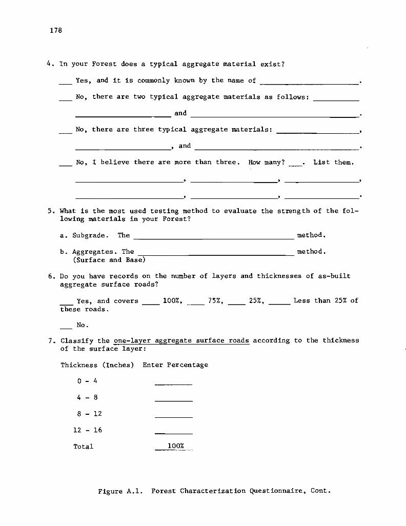
178
4. In your Forest does a typical aggregate material exist?
Yes, and it is commonly known by the name of ________________________ _
No, there are two typical aggregate materials as follows:
and ----------------------- ----------------------------------------No, there are three typical aggregate materials:
_________________________ , and ________________________________________ __
No, I believe there are more than three. How many? List them.
----------------------------,
5. What is the most used testing method to evaluate the strength of the following materials in your Forest?
a. Subgrade. The method. -----------------------------------------b. Aggregates. The method.
~--------------------------------------(Surface and Base)
6. Do you have records on the number of layers and thicknesses of as-built aggregate surface roads?
Yes, and covers these roads.
No.
100%, 75%, 25%, Less than 25% of -----
7. Classify the one-layer aggregate surface roads according to the thickness of the surface layer:
Thickness (Inches) Enter Percentage
0-4
4 - 8
8 - 12
12 - 16
Total 100%
Figure A.l. Forest Characterization Questionnaire, Cont.

179
8. Classify the two-layer aggregate surface roads according to the thicknesses of:
a. Base Layer b. Surface Layer
Thickness, in. Enter Percentage Thickness, in. Enter Percentage
o - 4 0 - 4
4 - 8 4 - 8
8 - 12 8 - 12
12 - 16 12 - 16
+ 16 + 16
Total 100% Total 100%
9. Has some system been implemented in your forest to measure traffic (number of applications), or are you going to implement some type of system during this year?
10.
_____ Yes, and the system(s) is (are) ________________________________ __
which cover(s) 100%, 75%, 50%, than 25% of the aggregate surface roads.
____ No.
-----25%, Less
What are the different levels of Average daily Traffic (ADT) for the for the Aggregate Surface Roads in your Forest?
From 0 to 50 VPD* for % of these roads.
From 50 to 100 VPD for % of these roads.
From 100 to 200 VPD for % of these roads.
From 200 to 400 VPD for % of these roads.
More than 400 VPD for % of these roads.
Total 100 %
*VPD: Vehicles per day in both directions.
Figure A.l. Forest Characterization Questionnaire, Cont.

180
11. Classification of the traffic in your forest by gross vehicle weight (GVW).
Passenger cars and pick-ups %
Trucks from 10,000 to 30,000 lb %
Trucks from 30,000 to 100,000 lb %
Trucks from 100,000 to 200,000 lb %
Total 100 %
12. Do you think that the topographic conditions of your Forest are all the same?
Yes, they are uniform throughout the Forest and could be described
as:
No, I think we can identyfy different topographic conditions our Forest as follows:
in % of the Forest area.
in % of the Forest area.
in % of the Forest area.
(If you need more space, please use the back of this sheet.)
13. Do you think that the environmental conditions of your Forest are all the same?
in
Yes, they are uniform throughout the Forest and could be described
as:
No, I think we can identify different environmental conditions ---- in our Forest as follows: (You may answer in terms of annual pre
Cipitation and/or temperature.)
in % of the Forest. -------------------------------------------in % of the Forest. -------------------------------------------in of the Forest. ---------------------------------------
Suggestions:
Figure A.l. Forest Characterization Questionnaire, Cont.

181
TABLE A.I • NATIONAL FORESTS CONSIDERED IN THE SURVEY AND THEIR REPLY INCLUD-'ING VALUES OF MEAN ANNUAL PRECIPITATION AND HEATING DEGREE DAYS.
National Forest Mean Annual Heating Com- Precipita- Degree
Reg. State No. Name p1eted tion. in. Days
1 Idaho 1. Clearwater xes 27 72 000 2.. Idaho Panhandle NFS. Xes 27 72 000 3. NezEerce xes 25 8 2 000
Montana 4. Beaverhead xes 14 10z000 5. Bitterroot xes 19 72 500 6. Custer xes 14 92 500 7. Deer10dge xes 19 8 2°00 8. Flathead yes 19 8 2500 9. Gallatin yes 14 10z000
10. Helena yes 14 8 2 000 11. Kootenai yes 19 8 2 500 12. Lewis & Clark yes 14 8,000 13. Lo10 xes 19 8 2 000
2 Colorado 14. AraEaho & Roosevelt xes 16 92 500 15. Grand Mesa, Uncompah-
gre and Gunnison yes 17 9 2000 16. Pike & San Isabel no 14 10 z000 17. Rio Grande xes 15 10 z000 18. Routt xes 17 92 000 19. San Juan xes 17 8 2500 20. White River yes 16 8 2 500
Nebraska 21. Nebraska yes 19 7 J OOO South Dak 22. Black Hills yes 20 72 500 Wyoming 23. Bighorn ;yes 12 82 000
24. Medicine Bow ;yes 13 8,000 25. Shoshone ;yes 11 10,500
3 Arizona 26. AEache-Sitgreaves xes 14 52500 27. Coconino yes 14 6,000 28. Coronado yes 13 22500 29. Kaibab yes 14 5 2500 30. Prescott ;yes 14 4 2 500 31. Tonto no 18 5 2500
New Mexi- 32. Carson ;yes 15 8,500 co 33. Cibo1a no 13 5 2500
34. Gila yes 13 6 2°00 35. Lincoln yes 10 4 2500 36. Santa Fe yes 16 4 2500
4 Idaho 37. Boise yes 27 8 2 500 38. Caribou no 15 82 000 39. Challis no 27 8,500 40. Payette yes 27 82500 41. Salmon yes 9 72 500 42. Sawtooth ;yes 27 72 000 43. Targhee yes 12 8 2500
Nevada 44. Humboldt no 8 62 500 45. Toiyabe no 8 62 500
(continued)

182
TABLE A.I. NATIONAL FORESTS CONSIDERED IN THE SURVEY AND THEIR REPLY INCLUD-ING VALUES OF MEAN ANNUAL PRECIPITATION AND HEATING. DEGREE DAYS.
Mean Annual Heating National Forest Com- Precipita- Degree
Reg. State No. Name pleted tion, in. Days
4 Utah 46. Ashle:l :les 19 72 500 47. Dixie no 12 5 2 500 48. Fishlake no 10 5 2 500 49. Manti-Lasal :les 10 5*500 50. Uinta :les 16 SzOOO 5I. Wasatch :les 19 9 2 000
Wxoming 52. Bridger-Teton xes 20 10 2 500 5 CaHfor- 53. Angeles no 18 3,000
nia 54. Cleveland :les 17 3 2000 55. El Dorado xes 20 8 2 000 56. In:lo :les 9 6 2000 57. Klamath :les 41 5 2500 58. Lassen xes 35 6 2000 59. Los Padres :les 21 2,500 60. Mendocino xes 41, 4 2500 6I. Modoc xes 40 6 2 500 62. Plumas xes 40 7 2 000 63. San Bernardino xes 18 3 2500 64. Seguoia xes 9 62500 65 ... Shasta-Trinitx xes 41 4,000 66. Sierra :les 10 8 2 000 67. Six Rivers xes 41 4,500 68. St. Anislaus xes 9 8,000 69. Tahoe xes 20 72000
6 Oregon 70. Deschutes Xes 33 7 2500 7I. Fremont xes 20 72 500 72. Malheur no 19 7 2 000 73. Mt. Hood xes 52 62 000 74. Ochoco Xes 13 7 2 000 75. Rogue River Xes 30 6 2500 76. Siskixou xes 75 5 2 000 77. Siuslaw xes 75 5 2000 78. Umatilla :les 19 6,500 79. UmEgua xes 30 5 2500 80. Wallowa-Whitman xes 19 6,500 81. Willamette yes 52 6,000 82. Winema yes 30 6,000
Washing- 83. Colville yes 20 7,000 ton 84. Gifford-Pinchot yes 63 8,500
85. Mt. Baker-Snogualmie xes 90 8 2 000 86. Okanogan xes 34 8 2 000 87. OlymEic xes 102 7 2000 88. Wenatchee xes 34 72 500
(Continued)

183
TABLE A.1. NATIONAL FORESTS CONSIDERED IN THE SURVEY AND THEIR REPLY INCLUD-ING VALUES OF MEAN ANNUAL PRECIPITATION AND HEATING DEGREE DAYS.
Mean Annual Heating National Forest Com- Precipita- Degree
Reg. State No. Name p1eted tion, in. Days
8 Alabama 89. William B. Bankhead ~es 52 3 2500 90. Conecuh yes 56 1,500 91. Talladega ~es 52 2,500 92. Tuskegee no 53 22 000
Arkansas 93. Ouachita ~es 50 22500 94. Ozark ~es 45 32500 95. St. Francis ~es 49 32 000
Florida 96. Aea1achico1a ~es 50 32000 97. Ocala ~es 50 3 2000 98. Osceola :fes 50 32 000
Georgia 99. Chattahoochee no 51 32500 100. Oconee no 47 2 2500
Kentuckx 10l. Daniel Boone :fes 45 4 2 000 Louisi- 102. Kisatchie no 56 2,000
ana Missis- 103. Bienville ~es 51 22 000
sippi 104. Delta :f~s 50 22500 105. Desota :fes 59 1 2 500 106. Ho11~ Serings :fes 52 3 2000 107. Homo chit to :fes 55 1 z500 108. Tombigbee :fes 52 2 2500
North 109. Croatan :fes 49 2z000 Caro- llO. Nanjaha1a ~es 54 4 2000 1ina 111. Pisgah :fes 52 4 2000
112. Uwharrie ~es 46 32 000 Puerto 113. Caribbean 110
Rico South 114. Fr ancis Marion no 45 22 000
Caro- 115. Sumter no 45 2 2 500 Tennes- 116. Cherokee yes 48 4,000
see Texas 117. Angelina no 45 22 500
118. Dav:f Crockett no 45 22 500 119. Sabine no 45 22500 120. Sam Houston no 45 22 000
Virginia 121. George Washington :fes 41 42500 122. Jefferson ~es 43 4 2500
9 Illinois 123. Shawnee :fes 43 4 z000 Indiana 124. Wayne-Hoosier yes 40 5,000
& Ohio Michigan 125. Hiawatha ~es 29 8 2 500
126. Huron-Manistee :fes 29 72 500 127. Ottawa :fes 32 9,500
(Continued)
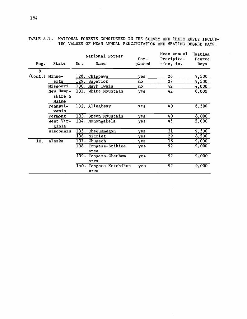
184
TABLE A.1. NATIONAL FORESTS CONSIDERED IN THE SURVEY AND THEIR REPLY INCLUD-ING VALUES OF MEAN ANNUAL PRECIPITATION AND HEATING DEGREE DAYS.
National Forest Mean Annual Heating Com- Precipita- Degree
Reg. State No. Name p1eted tion, in. Days
9 (Cont. ) Minne- 128. ChiEEewa xes 26 92 500
sota 129. SUEerior no 27 92 500 Missouri 130. Mark Twain no 42 4,000 New Hamp- 131. White Mountain yes 42 8,000
shire & Maine
Pennsy1- 132. Allegheny yes 40 6,500 vania
Vermont 133. Green Mountain Xes 40 82 000 West Vir- 134. Monongahela yes 45 5,000
ginia Wisconsin 135. Cheguamegon xes 31 92 500
136. Nicolet xes 29 82500 10. Alaska 137. Chugach xes 18 9 2000
138. Tongass-Stikine yes 92 9,000 area
139. Tongass-Chat ham yes 92 9,000 area
140. Tongass-Ketchikan yes 92 9,000 area

185
TABLE A.2. FOREST CHARACTERIZATION QUESTIONNAIRE. QUESTION NO.3 TYPICAL SUBGRADE MATERIALS. ANSWERS SUMMARY LIST.
Code
1
2
3
4
5
6
7
8
9
10
11
12
13
14
15
16
17
Sub grade Material
Gravels General
Sandy Gravel
Clayey Gravel
Silty Gravel
Alluvium
Sand General
Gravelly Sand
Clayey Sand
Silty Sand
Clay General
Clay Low Compressibility
Clay High Compressibility
Clay Shale
Silt General
Silt Low Compressibility
Silt High Compressibility
Organic Sil ts
Including
gravels, granular material, gravelly stoney materials, glacial gravels, glacial moraine, glacial till, chert, gravels: GP/GM/GC, glacial outwash.
clay and gravel, clayey gravel or clayey sandy gravel, GC
Silty gravel, silty sand gravel, GM
alluvium, fluvial deposits
sand, sandy soils, glacial sand, granitic sand
sand and gravel, sand or gravelly, sand well graded, SW, SP, SU
clayey sand or clayey gravelly sand, coa:cse sand, graywacke, SC
silty sand, silts and sands, sand shale, silty sand or silty gravelly sand, residual soil, SM, sandy silt
clayey soils, clay, glacial clays, A-6, A...,.7
CL, inorganic clay mixtures, lean clays, sandy clays, gravelly clays, low plasticity clay, silty clays
clay high plasticity, fat clays, expansible clays, CH
silty soils, silts, glacial silts, A-4, A-5, palouse silts
silts. sandy silts, gravelly silts or diatomaceous soils, lake bed sediments, lacustrine silts, phylitic, loess, ML
silts high plasticity, micaceous clay or diatomaceous soils, serpentinite, inorganiC silts, MH, plastic silts, clayey silts
organic silts or lean organic clays, OL
(Continued)

186
TABLE A.2. FOREST CHARACTERIZATION QUESTIONNAIRE. QUESTION NO.3 TYPICAL SUBGRADE MATERIALS. ANSWERS SUMMARy LIST. (Continued)
Code Subgrade Material
18 Loams General
19 Sandy Loams
20 Clay Loams
21 Silt Loams
22 Volcanic Materials
23 Organic Materials
24 Weathered Rock
25 Rock
26 Information Not Available or Sufficient
Including
loams, Gila conglomerate material
sandy loams, loamy sand, sandy clay loams
clay loams
silty clay loams, silt loam
cinder, ash
wet meadows, muskeg, organic materials
stone fragments, weathered rock, broken rock, partially decomposed rock
argillaceous dolomites, granite,decomposed granite, granite gruss, shale, limestone, quartzite soil, quartz feldspar, gneiss, micaschist soil, basaltic soil, sandstone, andesite soils material, rholite soil material, datil soil material, sedimentaries, metamorphic, bedrock, scoria, argillite, schist, yeso formations, igneous (intrusive & extrusive), volcanic deposits, pumice, hard pan, quarry rum shot rock

187
TABLE A. 3 • FOREST CHARACTERIZATION QUESTIONNAIRE. QUESTION ~"'(). 4 TYPICAL AGGREGATE MATERIALS. ANSWERS SUMMARY LIST.
Code Aggregate Material
1 Natural Deposits
2 Volcanic Materials
3 Weathered Rock 4 Volcanic Rocks General
5 Pegmatite
6 Diorite
7 Andesite
8 Granite
9 Basalt
10 Gabbro
11 Diabase
12 Scoria
13 Rhyolite
14 Metamorphic Rock General
15 Quartzite
16 Schist
17 Phyllite
18 Gneiss
19 Seppentine
20 Marble
21 Sedimentary Rock General
22 Limestone
23 Sandstone
24 Caliche
25 Metasiltstone
26 Mudstone
Including
ri"er gravel, river run, stream deposits, outwash gravels, clay gravel, glacial deposits, glacial till, boulder conglomerate (consolidated gravel), terrace gravels, natural gravels, chert (GP), natural bank materal
igneous, cinders
tuff, metavolcanes, volcanic outcrops
(Continued)

188
TABLE A.3. FOREST CHARACTERIZATION QUESTIONNAIRE. QUESTION NO. 4 TYPICAL AGGREGATE MATERIALS. ANSWERS SUMMARY LIST.
Code Aggregate Material Including
27 Shale
28 Graywacke
29 Argillite
30 Crushed Stone not Spe-cified
31 Information Not Avail-able or Sufficient

189
TABLE A.4. FOREST CHARACTERIZATION QUESTIONNAIRE. QUESTION NO. S.a MOST USED SUBGRADE MATERIAL TESTING ME'TIiOD. ANSWERS SUMMARY LIST.
Code Met hod
1. Resistance R-Value and Expansion Pressure of Compo Soil
2. CBR (AASHTO T-193)
3. Density Measurements Proctor (AASHTO T-99/S.S lb Rammer & 12" Drop) Modified Proctor (AASHTO T-1SO/10 lb Rammer & lS" Drop) In Place Test Using Sand Cone Method (AASHTO 191) In Place Test Using Rubber-Balloon Method (AASHTO 205) In Place Using Nuclear Methods (AASHTO T-23S)
4. Moisture Measurements Using Calcium Carbide Gas Pressure (AASHTO T-2l7) In Place Test Using Nuclear Methods (AASHTO T-239)
5. HVeem Stabilometer
6. Sieve Analysis
7. Field Evaluation
S. Soil Support Using PI and Haterial Passing No. 200 Sieve
9. None
10. AASHTO Methods General
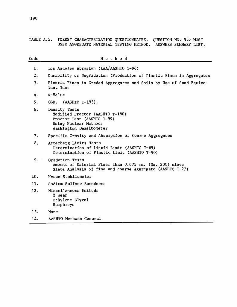
190
TABLE A.S. FOREST CHARACTERIZATION QUESTIONNAIRE. USED AGGREGATE MATERIAL TESTING METHOD.
Code Met hod
1. Los Angeles Abrasion (LAA/AASHTO T-96)
QUESTION NO. S.b MOST ANSWERS SUMMARY LIST.
2. Durability or Degradation (Production of Plastic Fines in Aggregates
3. Plastic Fines in Graded Aggregates and Soils by Use of Sand Equivalent Test
4. R-Value
5. CBR. (AASHTO T-193).
6. Density Tests Modified Proctor (AASHTO T-180) Proctor Test (AASHTO T-99) Using Nuclear Methods Washington Densitometer
7. Specific Gravity and Absorption of Coarse Aggregates
8. Atterberg Limits Tests Determination of Liquid Limit (AASHTO T-89) Determination of Plastic Limit (AASHTO T-90)
9. cGradation Tests Amount of Material Finer than 0.075 mm. (No. 200) sieve Sieve Analysis of fine and coarse aggregate (AASHTO T-27)
10. Hveem Stabilometer
11. Sodium Sulfate Soundness
12. Miscellaneous Methods % Wear Ethylone Glycol Humphreys
13. None
14. AASHTO Methods General

191
TABLE A.6. FOREST CHARACTERIZATION QUESTIONNAIRE. QUESTION NO.9 TRAFFIC MEASURING SYSTEMS ANSWERS SUMMARY LIST.
Code S Y i3 t e m
1. None
2. Traffic Counters in General
3. Inductive Loops
4. Electronic Counters
5. Magnetic Counters
6. Manual Counters
7. Pneumatic Counters
8. Random Sampling
9. Relation with Volume of Timber

192
TABLE A. 7. FOREST CHARACTERIZATION QUESTIONNAIRE. QUESTION NO. 12, TOPOGRAPHIC CONDITIONS. ANSWERS SUMMARy LIST.
Side Slope Code Topographic Condition %
1 Flat to Rolling o - 15
2 Gently Rolling to Hilly 15 - 30
3 Mountainous 30 - 50
4 Steep Mountainous +50
5 Information Not Available
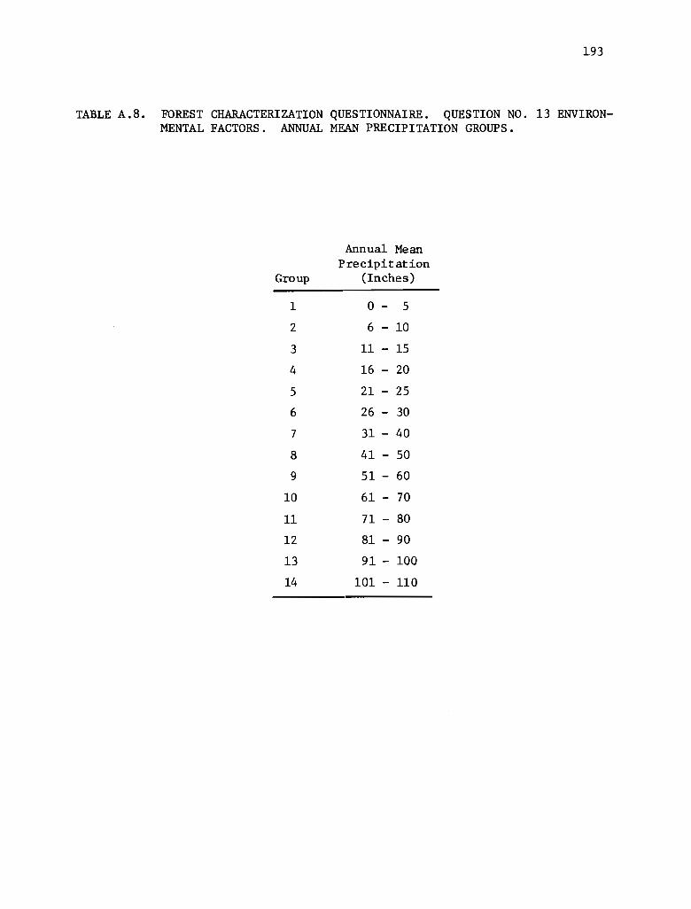
193
TABLE A.8. FOREST CHARACTERIZATION QUESTIONNAIRE. QUESTION NO. 13 ENVIRONMENTAL FACTORS. ANNUAL MEAN PRECIPITATION GROUPS.
Annual Mean Precipitation
Group (Inches)
1 o - 5
2 6 - 10
3 11 - 15
4 16 - 20
5 21 - 25
6 26 - 30
7 31 - 40
8 41 - 50
9 51 - 60
10 61 - 70
11 71- 80
12 81 - 90
13 91 - 100
14 101 - 110

194
TABLE A. 9. FOREST CHARACTERIZATION QUESTIONNAIRE. QUESTION NO. 13 ENVIRONMENTAL FACTORS. HEATING DEGREE DAYS GROUPS.
Heating Group Degree-Days
1 o - 1000
2 1001 - 2000
3 2001 - 3000
4 3001 - lLOOO
5 4001 - 5000
6 5001 - 6000
7 6001 - 7000
8 7001 - 8000
9 8001 - 9000
10 9001 - 10,000
11 10,001 - 11,000
194
TABLE A.9. FOREST CHARACTERIZATION QUESTIONNAIRE. QUESTION NO. 13 ENVIRONMENTAL FACTORS. HEATING DEGREE DAYS GROUPS.
Heating Group Degree-Days
1 o - 1000
2 1001 - 2000
3 2001 - 3000
4 3001 - [.000
5 4001 - 5000
6 5001 - 6000
7 6001 - 7000
8 7001 - 8000
9 8001 - 9000
10 9001 - 10,000
11 10,001 - 11,000

195
TABLE A.10. RELATION BETWEEN THE SUMMARY TABLES AND THE QUESTIONS OF THE FOREST CHARACTERIZATION QUESTIONNAIRE.
Sununary From Table Question Number Number
1 1
2 1
3 2
4 7
5 8
6 6
7 10
8 11
9 9
10 3
11 4
12 5
13 12
14 13
195
TABLE A.10. RELATION BETWEEN TIlE SUMMARY TABLES AND THE QUESTIONS OF THE FOREST CHARACTERIZATION QUESTIONNAIRE.
Summary From Table Question Number Number
1 1
2 1
3 2
4 7
5 8
6 6
7 10
8 11
9 9
10 3
11 4
12 5
l3 12
14 13

!!!!!!!!!!!!!!!!!!!"#$%!&'()!*)&+',)%!'-!$-.)-.$/-'++0!1+'-2!&'()!$-!.#)!/*$($-'+3!
44!5"6!7$1*'*0!8$($.$9'.$/-!")':!

APPENDIX B
FOREST CHARACTERIZATION QUESTIONNAIRE,
NATIONAL SUMMARY
197

!!!!!!!!!!!!!!!!!!!"#$%!&'()!*)&+',)%!'-!$-.)-.$/-'++0!1+'-2!&'()!$-!.#)!/*$($-'+3!
44!5"6!7$1*'*0!8$($.$9'.$/-!")':!

'" ... .. ... .. ::> ., ... co
'" .. . >. ..... . >'" ., ..
o ., ... o .. 0'" .. -... 1" .. 2 ..... 0 ..
> 20 OU
~ .. ::! ... -..... ... "2 .... 0 UM ~ .... _z
··:·z:······················· ... ························ .... • o • • z __ .-~ .• ~~.C .• -~O-~~.~ .. _~~~_ .. ~ .. ~.~_~ ... ~eC~.~Q.N.~~.M .• 0 · ........................................ ~ ........................... ., .................................... .. . mz___ ~ - N _ _ _ _ _ _ N _N ____ _ ...... • 1& •• :. : ................................................... . · . • m ••• 5~~5~5~ •• _._M •• S •• _ ••••• C ••• ~ •• O •• __ •• ~~ ••• ~S.S~ •• • .... • ............................................ ~ .................................. e ....................... .. • ~ •••• _N~~.~O._N.~O __ M •••• ~OQNOO~M ••••• N •• ee_M.~ •••• ~.N -- ••••• NO.NN~O-N~.N._~~.M_.~NN._C_ •• N._~.OO~~._N~.~ •• N_ .~ •• N ••• O •• ~.-.~O~MOe~._NQM.~O.N.M ••• O~ •• C~_C~.M~~~CM.~ • .~. __ NN_N _~ O-MN_N __ M N __ N_N __ ._N~ __ N____ N_.M NOM ..... ... ... • 0 .... · . · • 2 .20 .MM · .. ..... ..... 2 ... · .. · ... .... -..... .::::J", ....... .2M .::::J:I:
'"': u ••• · ... Z .20 .... --· .. ..... ..... 2
::l:':. ... . ~
· ................................................... . · .................................................. . •• IS~O.N.&~S~.~ •• mm._05 •• 5S ••• IS •• 5~5.~~SS~S5~s.5 •• mm5 .................................................... •••• ~~~~ ••• N~M •• ~~_~ •• ~ •• OO~M •• ~ •• M.~ •• ~_~ •• ~_m5CS.m M •• _MM •• ~ ••••• ~.M __ ~O .~--N~~~.~ •• 0~ •• ~.Q_~~~.M_~.55 ~ •• ~.~M_.S_OMMMN __ ••• ~N~~M~fIIII •• OO.$ •• ~.~$~~~._O~.~Q~ N. ____ N _N N_MN_N_ N ____ N_ ~-NO_______ _ __ N NN~
· .................................................. . · .................................................. .
:~; ~~~~~~~~~~~~~~~~~~~~~~~~~~~~~~~~~~~~~~~~~~~~~~~~~~~~ • .e~ •• E~~~.M~~.~ ••• OON •• ~M~.~_ •••••••• OM.O •• N.M •••• ~& ••• ..... ~~ 5 ••• N~~M ••• M._._N.MN~M •••• S O •••• ~~NSM~ ••• M ._ M.~ .O. __ •• N~ ._0 .~._M_M._O._~_~O 0 _N_N M. ~ ~._ NN • ."Z._ N _ ~-· .e_. · ... . .. . ..... . . . . . . . . . . . . . . . . . . . . . . . . . , ................................. . .. . ••• 7. • .ZO • .. > ........ . · . .... . • ~ • IS ... • • ...... Z. • .. S • · ....................................................... . · ... . • ..... ••••••••••••••••••••••••••• O ••••••••• IS ••• M •• ~$ •••• Na. .. ............................................................... . • .~_ ••• IS.aM ••• ~ ••• _ ••••• _.m •••• ~.-~~ ••••••• ONN •• ~ •••• ~O.~ • .u., •• N ._11\ ~ _ -. M _. NM. eo •• · .c.... ~ filii • · .... -' . · .--. • • =- Z • • • e .... .wr: .. . · ....................................................... . • .22. · ._0. · . -. · .. ~. · .......... • •• 2 • · ................•....................................... .. . .. . •• • •• a.~ ••• ~ •••• ~ •••••• N ••• aa-••• _ •• O •• ~o •• e •• -.~ •••••• · . ~ - ................ .................................................... ......... . • .~_ •••• & •• OM_.~ •••••• _ ••••• ~ •• O •• _O •• ~_ •• ~_~~M.~.~~O •• • .... w.~ _~ N~ 0 ~_._ MN O. _.O~ N ._OC~~N.N-eNMN~-N • • .%-'. --• • lit. _ •
• e z • ... -. · .. ......................................................... • • · . • • 2 • • ~ ~J • • Z ~" • • 0 ~. ~ • .... >-Z ... • • ~o >-• • _ _u .. • • ~ • OZ'" Z • • _ OJ :. _ 0 til.... . .. ... _. .. _ 0 " -' ~
~:~ :~: ~~ ~ ~ .:~ ~ ~ e ~ : ~oc :0 • .,. .~ ....... o eoz _ ~Z z_ ... _ ~ ... _oo ~ ~ :z ... IZO .z • .c .c~U%. oc_ .... o~ ... ..... ZZZZ ZO ~ Z~ ~ ~~ ~ Z ....... x 0_ : ... :z ::~~:~:~r:;:. :o:~~~:.~~~r;:=~~ ~c~:~g:~!c~=~~ =~:~u: ••• .c~a>~~.~-'~~MO.Z ~ ~.u%_.UOO. __ cu~ __ Z~.-'~~co>oo~_ OOZ
:0: :~:=::~=~~~g~S::~~~;:~=~~:~~:::~~~o~~:::~~:~~-';::~~g3 •• .u_zemuc~e%.~-' ... g •• ~~Z •• z_cu~.aug-'-.a--~ .. ~~~.u ... -.-'~zza :~: .. : .........••.•....•......••..••••......•.......•• .... : :~ :_N .... ~.~ .... _N~.~~., ... _N ... O~.~ .... NO~.~ .. _N ..... $_NO~.~ .... -N • .Z • _________ N~~NNNNNN~M~M~M~OO.O.O~.~~ •••• ~ ••• .. . : :.«: •••••••••••••••••••••••••••••.••••.••..•••••••••••••
199

200
... tI ................................... « .................. tI ......................................................... .. · . • « •••••••••••••• ~~.~ ••• OO.~~_~ ••• N.N_~~M __ ._.~.~ •••• M_._ •• ~._N.: :
• .......... e_ ............................ e. • • • • • • • • • • .. .. • • • • • • • • • .. • • • • • • • ... .. N ......... ______ NN ___ __ N _ .. .. · . ............••.........•.............•.•....•................ : .: · . ••• S.m6&S.N.~NS.~ •• ~ •• ~N.O~ •• ~_N.~.N~NN.O~$ •••• S •• &~O.~~ •• &.&: _! · . " .............. , . . .. . . . .. .. . .. .. . . . . .. .. . . .. . .. . . . .. .. .. . .. . . .. .. . . . . .. . . . .. . . . ... . .. . ~~._m-.SMM.C~.-.•• &.~ •••••• ~._ •••• ~ ••••• _Ne_~.~.N~ •• ~C.~C.~&. ~ • . ~.~.~~.--C •• M~._-.-••.•• _N~N •• ~ •• ~ •• N ...... __ ._ •• NON.~_ •• ~M •• M. ~M ••• ~N~.~~~ •• N.~~O •• O •• _.M •• O __ M._ •• ~NN_M.N.~ __ ~~.N.N •• __ ........ . --~_NNN •• ~NN~~~ ••• _ •• M_N~_ .N~N N N __ N__ __ _.~ • .. .. . .. ... . · . · . · . •..••...•....•...•...•.•...•.••.•.........................•.. : .: · "'. · .. · .. . .. .. . · . .. .. .. . •.........•....•.....•••.••............•............•••.••...... ... . •• ~S~~~SGS •• N ••••• SS ••• N ••• & •• _O •• ~~N~.~~.$~.5S •••••••• #S~&S~.~. · . . . . . . .. . . . . . . . . . . . . . . . . . .. . . .. . . . . . . . . .. .. . . . . .. . . . . . .. . . .. . . . . . .. . .. . . • N.&~S&&.N.~ •• mNM.~m.~NM.N.~. __ •• N~~_~.~_.s.~~m.~~&.~~~~~~.S •••• ~M •• N.~S~ ••• ~-.~ •• ~ ••• NC~~._&".N ••• N~N&~~.SC.~ •• _ ••••• ~~ •• ~ $ ••• • NN~~$._N._.~NS~_~~.~ •• ~~ON._.~~~ __ N~. __ ~N.~.~ .~.~_~ ~~o ~ ~. #. --"'_ IIIU_ ... ~___ _ ~ N_ __ O_N_ _ _ _. ~ • .. ... · -. · .. .. . . . . . . . .. . . . . . . . .. . . . . . . ... . . . . . . . . . . . . . .. . .. . .. . .. . . . . . . . . . : .:
: ..... : · .. · ... : N: .. .. ............................................................... : .: ...... ••••• $& ••• S.M~ •••• S ••• ~ .... _om.N ••• _ •• _ •• _ ••• ~ ••••••••• SNC •••••••• · ....................................................................... . •••• _.NC~~~.O~.N_ •••••• N ••••• NM_.~_N_.N ........ ~ •• _ ••••• ~ •• S._& ... . .• _N •• Q"'_ ••• _ •• &.SS ... __ " __ .S~.N~.~_.S.~ •• m~~~Q~ ••••••• ~.NN~&. ~.
~ •• __ ._~.~~._.N •• N ••• "" .~."N~N • ~ 0 O~N_ N_~"'_~ __ e. ._ ... N ______ ~N_~ _N_ __ •••
• • .. . · . . . . .. . . . . . . . . . . . . . . . .. . . . .. . . . . . . .. . . . . . . . .. . . . . . . . . .. . . . . . . .. .... .. : : · .. . · ... . · ... .. · . .. .. · . .. . . . . . . . . . . . . . .. . . .. . . . . . . . . .. . . . . . . . .. . .. . . . . . . . .. . . . . .. . . .. .. · . •••••••••• _."' ••••• m •••• ~.N ••••••• ~ •••• N ••••••••• mss._.~.m ••• S. ~ • .................................................. , ....................................... .. • ~ •. ~&N._. __ .. e.~ ... ~~~_~.~ ......... ~ ~ ... N.-~~.&~~.~._~ ....•. N.
_N. NoO_ •• , .. ,,'" "'._~ - N. _M ~N - _ .... ~__ N._ 10.'" .. ~. _ •• _ M _ ••• · .... · . · . .. .. · . .. .. . . . . .. .. . . . . . .. . . .. . . . . . . . . .. . .. . .. . . . . . . .. .. .. . .. .. .. .. . . .. .. .. .. · . .. .. : ,:: .. .. ................................................................... · . • ... 4O •••• & •• & •• ~.~_ ............ _.~ ••• ~ •••••••••• "N ••••••••• ~ •• _~._ ••••..• ........... , ................................ , ..................................................................... .
•••••• ~.N ....... N_~ •• C.~.N •••• ~~ .............. && •• ~ •• ~~~.& e ••• I0 ••••••• N .~ ....... N_ •••• N ••• N ••••• N • N NN __ "'N~ N • • ••
-_N _... IN - '" ~ - - : "': · . · .. .. . .............................................................. : .: · . c.. • • = c:'.. :-:: .. : : r d .... ...J Z ..... Z •• ,..J tuZ "'0 .....
i ~ : i~ ~ e .:.:.:: z ~ a~~:: :; ~ a: ~ ~~ :f .~!: ~ : ~ ~ = : : .. z ~~~: :
; E !!:. :=> i~ w&7z :: .. :;~ ~~ i:: : ... ..,:~ g ... : .. ~~!r: ~Yi:~: ..... I >...1 ...... 0 .0:.--, ..... ,..JO ....... "'z ... %~.% ... -' ....... z .... w .~%%:It' .:r;wz .. a: .... z ......... . ... _ ...... w. ~zoo > .. .J ... ss ... -'.¥aw"' ... ~ .... U ...1...1" 0 z ... % ...... ~.~ •• .., % u ... wu ...... . _O ..... *_..,ZOO"' ... _.J .... ~0 .. z_c ... oa .... %U% ...... OW> ....... ~"'"~ ... OOWZW .. 2.&W.ZZ~-' ............ z. ~ •• ZOU.ZO~._~G.J...JW> •• ZS4VWU • .J...J ... kZ .. C.JOm .... 4 .... SZ~oca .... w ... o.o.ODO. •
Z04WX ... Z •• % •• ~.a...J...Jz...J~ ... ~ZZZ ....... "'z ... ,..J • .Jrzc.Z ... c •• > .............. ,..J ... ZWU~ZZZ. z. c ... %ww .... W.~UO .... _~S .. _kC .... ~ • .J_cO~NaU_ .. w ... WQOO ...... Z~ ... Z ...... ~~%Z,..J.0%_%000 ...... ••••• m .. c.:r;o ••• ~~ •• SU.:It'OD •• ~OO ... OOQ.QC%% .... ua~uU~_X%ZCus .. aZUZU ........ :.J: ........•.......••.•...........•.....••....••.•••••......••.. ::: ::::~::~~=:=:~:~:;=::::::::~::::~;;;;;;;=:=~:S:~!;;~;e;;;;;;:: ~: · . ........................................••...•..................

.. ... .... -,. • ...... ~= .... .. %0 ...... .... ::0'"
Q .. -"' ... ,,'" 00 au ....... :1:% t-
o. o %
~ .. '" ....... _ .. IICZ .. 0 ._ .. 0" z
« «
_ •••• _G •••••••• N •• N •• MN •••• _··~· ••••••••••••• N.M ••••• _ •••• W.~ •• ft~ •••• - ••• - •• ~N_.M ...... ~ .. N •• _._N.~ ... ~.N .. _M •••• ~ •• -' II ........................................................................................................... .. _ ••• MM.M.M~ ••••• _~_ ••••• M.Mm •• _~ •••• M ••• _~N •••• ~._N •••••••
-'a ••• ~N-._.N_.~ •• _ ••• N •• ~._ •••••••• _M~.N •••• ft_~MMft •••• • N_ •• •••• NM._._.~.M ••• "M •••• M •••••• N •• _ •••• ~_ ••• N •• ~.~_ •••• ~~ •• M ~-' ••• N __ N_N __ O_ON ____ M N ____ M ____ •• __ NNN _____ OM .OM __ ••
o • t- • • «
« • ••••• - •••••••••••••• _MS •••••••••• a ••••• NM_ •• M._ •••••••••• u ••••• _.N •••••• M •••••••• N ••••••• ·_ ••••• __ .~ •••• M •••••• •••• .... II ................................................................................. . ••••• ~.~ .... & •• ~_~N.~ ... ~ •• c._ ... ~~~ ...• ~ ....... _ .... ~ ....... ~ ..
_~.~ •. _~M_.~ .••.... __ ~~~ .~ __ ~~.~ ..•. _N .... ~_._ .. ~M~~ ... ~ •. ...... ~ .. ~_ .... M~. ___ N •• ~~~ •• ~ ••••••••• _.N.~~~.~.~.~.M.~~~ _X.N. ____ N _N ___ N ___ • __ _ ~N_ ~_N~_______ _ ___ _ ._~_~_ ... "'. .. . :0 • • • ... . ~ . •• &&.~N ••• S~$~~_S&_ ••• ~&.ss~s~~sm~s.s._.m __ 5s&&&S55S&&~.&~ ~ ••••• ~ •• ~.~ ••• NN.~N •• ~ •• ~._ ••••••••• _~~. __ ._ ••••••••• ••••
~~ .. ----.---.-----~~ .. ,-----.-.------~~--------------- ----_. 4 •••• ~ ••••••• ~ •• ~_ ••••••• - ••••••• ~ •••• NMN_ •••••••••••••••• u=:==: __ ;~:.~==:~::;:=~;~:!~:-: !=:;::.~:.:c:: : :: ~:= :: ... ~_ _". N _ _ N_ ... ...... ... '" . • :~:::::::::::::::::i:::::::::::::::::::::::~::::::::=:I::::
... a •••••• ~ ••••••••••••• _ •••••••••••••••••••••••••••••••••• w •••••••••••••• N •• & •• _ ••••••••• NNN.NC •• S ••••• _~._ •••• ~.~ •• •• •• ~_~ • _ __.. N~ M •• • ~ •• N_. ~. _ • N _. _N
• N .... ~. 0::0 • •• • •
: •••• _.~ •••••• ~.~ •••• _._ •• _ •••• M ••••• N ••• ~ •• ~ •••••••••••• w~.~ •••••• ~ ••••• ~ •••• _ ••••... N •••• _._ •• _.~ ••••• N~.~ ••••••••
j •••••••• & •• ~.~ ••••••••••••••••••••••••••••••••••••••• •• ~ •• .4 ••••••• NN~ ••••• ~ •• _~ ••• __ ._ •••• _ •••• __ ~.N •• ~ __ ._._._ ••• ~ %.N M_.. • ._~_ .M c_ N~.~ _. .~.~~~ •• ~_~.~M~_ ••• ~~
>&._ _ ___ _M_ ___ _N •• ..... • • .. .. ..
• % : ~ ~~ • 0 W+ • • ~ >z ~ : • ::ft: 0 ,.. : ~ = g~ a : ~ ~ ~
~:.: c~ ~ «;W : ~ ~ : ~ ~ • ~! :=L~:~ :cz ~v .:~ Z~4= W~:Q~ ~ % : ~~g :~ ;:
~ •• ~~uz. O~~ •• L.~ 4 •• 7ZZ2 2C ~ ~~ ~ ~~ j Z.4~ % OM .~. : ::~::::~r~:~. ~C:~~~:Kg~~r~~:8~ 5~w=~gr~!.~:~~ =~:~v:=~:: ~~::,~!~=:~j~t~3::Q~2==~~=~~~:~::~~;=~~~:~~~:~:c~=:.~:~z5:: ... z:~~~==~Z~:~~~~:I.=:~~~=~~~~8::~=~:~:::::;~;:~~~~~3r~~:=~= .... .. .. . ~ :_N~.~.~&.s __ ~.~~ ••• _~~.~.~ ••. ~.~.~._N~ •• 5_~.~.~ ••• _~~.~. ~.. __________ ~N~~~N~_~~~~~~~ ••••• Q.~ .. ~_~.~ •••••• • ... 0. .. z. % ..
201

202
" " .... ~~N.~-.~~.~.~~_.~ .. ~··-.. __ ._~_ ..... _ .. _.~ .. ~.NN~~ ..... •• ~._._ •••• ~ •• __ .N •• ~NN.""~N.~ •• ".& •• ~ •• ~ •• ~.~ ••••••• N •••• ~ ........................................................... •••••• _~.".~ •• ~N •• N •• NN." ••• NN._~ •••• _.N~~._N •• _ ••• M~ •••••• ••• N-••• _~._._~ •• ~.N ••• ~N.M •••• N_._ ••• NM.~M.N.N •• ~_.~~~~." • •• - •• ~~_ •• _N~ ••• ~._.N.~~N._ ••• N •• ~NN_"_".~_N ••• N.N ••• _.04 •• NN" •• ~NNNN~ •• ~- •• ~_N~_ 4N"_ N _ N __ NN_ _ _N_ •••
"Po "N
" " • • :==:::::::::::~::::::=:~::~:::=:::::~::::::::=::::~:=:I:::: .......................................................... -. .. . . ••••• N.~ ••• N ••••• MNM.N ••• __ .~."._~~~_ •••••• NN ••••• M._ ••••• ~ ~ N.N •• Po •• M_.MM.~._.N •••••• M.N_ •• N.N.Po ••• N.~.NPo_ •• M •• M_ •••• Po .N.-N.-.PoN.~N •••••• ~ •• N.-._M~ __ NM. __ ~N •• ~ •••• M_M ••• _M ••• · • NN~~--- _. N_ _ ___ N_ _ _ ___ _ ••
.~ .-· · · .. && •••• ~esss ••• C.SS~ •• #~_~~~~.N~N.&~ •• &~~~ •••• S~& ••• N_S •• 5 •• •• N.~.M.M~ •••• ~ ••• _.~~_~ •• _ ••• _ •• _._ ••• N~~ ••••••••••• ~ •••• ~ . ---- --- -- ------- --------- -_ .. _ .. ------ _ .. -- --- ---- -- ----- --..... ~.~ •• ~~_.~ •••• ~.N.M_ •• N •• ~.N~.~ •• ~.~ •••••••• _ •••••••••• ~ •• M • ~.m •• NMe •• _.N~._.~_ •• N~_ •• N~ •• ~ •• _ •••••••• Poec~ •••• _ •• ~N~S"N •• • _M~N •• M •• _.~~~N ••• ~M ~.~.N.N ~ ~ • 4NN_ ~~.M_._ •• _ ._ ••• N ______ N __ ~ _NN -- -- _.~ N
.Po • • .. .. · •••.••••..••••. a.~ .•.••••....•••••••••...• ~ ..• & ••••• N ••••• ~ •••••••• M •••••••• N.N •••••••••••••••••••••• ~ •• ~ •• _ ••• ~ ••••• ~ ......................... , .................... _ .......................................................... . • N •• ~. __ .S •••••• M •• _~ ••••••••••••• & •••• ~ •••• ~ •••• ~ ••••••••• ~~= ~ ••• ~=N. - N! ~.-.~ N ~ .~-~ N ••• ~~ :: N ...
• • " • • • •• & •••••• W.N~ •••••• N ••••• ~ ••••••••••••••••• - ••••••••••••••• •••••• N.N ••••••••• - ••••• ~~ •••••••••• ~N._ •• ~ ••••••• N ••••••• _ '';'': ...... _ ... ,., .. .: ....... N ..... ~ .. .: .;-~,,: •• .:.:~_-...... ,:,:-.: M .. C ... fS ...... • ..... ~ ..... a .... · ... ,:.: ....... ::.: .... .; .... .: ..... :~.. ;: .~.N~.N.M ••• _N_ ~.... _ N • N ~~_N~~.. . N__ •• ~_ ~ 0_ _N N_. • - ~ •• •• • .. .. · · · cc •
~ c =. ~:c:~
~ ~~ ~ ! ~ ~ ~ z z ;;ai~ % %0 ~ ~ e ~ z «w _ _ _x%.
...
• ~ ;:: x • J
• :: ~~ t .!. ~ ~ .: % :!:; :. :'cz ~~~: ...... •• ~ ZW". ~ ~o ~ _0 Z • • _ z z~o ~%w.w c .~. ~ .~.. ~+ .u ow «~~ cz c z ~~~w. .u¥ ...... Z ~~ :~C :~ ...... :: ~c::ur~z:+; cc~ ~~:z+~:s~~~;; ;~~~~~~z~:::; ~ ;:~~~g:~~~~~~::~g=g~~~B~X~4S~:4~>~~:~:~=:~:~~:~w~z~~~~::::~ ~ M:~#~zf~=~~:jj~~~~::::~~:~~~;~~~j~:~::=gt:~:::!:~:f:Bgrll: ~ H~.~~~Uo __ rz. __ OH~WJ~.O~~&U_._~~OOOC_S%~~%._~~%%~.O%_%000. ~
•• ~o~rou •• ~~ •• 2UQEOO.CUOO.OO~COOZZ~U&~u.~ •• %Xou ••• ruzu~~~:~ 0 .. · ~ ... _~._.~ .•• _N~ ... ~ .•• M .• ~._~._.~_._N._~~ .•• ~C_N~ .•• ~ .... ~ ••• ~~~~~~~~~ •••••••••••••••••••••••• ___ N~NNNN.N~~~M~~~MM ••
_____________________________ .0
· ... .. z ~ U
'" ... It.

~HtDN'L Oil! L1~! , TWO Ll.U.
COVU1Nil I 11 'O~UTl. unn.4 4\; \ !'EACENT UUI.' B,' _EACENT
203
'* •••••••••••••••••••••••••••••••••••••••••••• _.-••••••••••••••••• -.-••• - ••• - •••••••• -•••••••• * ••• _ •••••••••••••••• '* •• '* '* ••• '* ••• '* '*;, '* •• '* •• • 'OA!IT. ON[ LlN! •• TWO L'''ES • .... HlM! • "'"'L' * I~ Tar I T.1ft .'GAEG.T!_ U"SU.' t. TnTil •• "PWAL T • S. Ti(f' T. '* lGGWfroJ TJE '* UNSUQ" • TOTlL
• '''IL'''' • C'4TLJ.S\ • ("'fLEI' • ,;.all"S,' fIolILf'" •• "1'ltES)' (loITLtS). (tolTl.ESl '* (MILEI) ....................................................................................................................................... • 1 C:L!'RWllfR • 1ft;. e,_ • ."~0. 1~1'.3. ".'.5 '.,5 e,0 -."... .,0 • 1":' • I 1'''''.IT.''''ur. lOW! • '.' P,' • 2Ie,_. 4111".p * oi5'.' til., 0*~ '.0 '.0: II,. *
I N[ZI'!I:CI .;e • '1.1 15;0.. • .... ~ * HUII'.".* o!.0 '8." "IIj.R rt.~ "el," • o 8f'\J!I:HI'() .. ',~ • I.' 58, ... ')'~.' lJe'.'.. 'l.1 e.e Q.1Ij '-.'" 21 •• * , 81TTrl:I:OOT • ',1 • e.1 • I'.' ""*' 1',e~I.. Se.' 8,0 ,a. 18.' ".l .. • tuaT[1: e,e .. 1.1. 1'1,_ 18)'."" 120e,' e.0 i'1.'" 223. t "'"."'" 10',1 * , orIIlLOOG! .,. • ".0.. ".2,5. 1''''.'. 1'1'!i',. 18,t ~.~ U.I tl.P 4'~2 *
• • "L'T~!'O '1,1 8.q. la,;,. 2t~J.l.'OI 150'.0,.. .i!~.7 "'.~ a1.1 O.0 '],1 * • • IULL'TIN .,~ • 6.111 • ..... 6''''~ * "1:,".. t.1Ij ".'01 O," GJ.~ ',II§ * .. lt1 HELEN' fI,1II • ,,~ ., S5,. ' •••• 111.. 11'1,'.. O.' 1.8 ~.1 I.VI '2.t • II .OOTfNiY e., • "0," 1'&0.' IU_,_. ns..... .'.0 15_.", ze.~ 0.~ lI5.' • • II Lfwll. CL'stl( 't~ • I.t. 11',' 41 •• ,. '!.','.. 1.1" 8<~ ]].8 2J.\ 6f!,a. • IS LOLO .,e .. ..1. 1'1',6. il"."'. .(ne.1 *. '''.1'' la.e li10.0 I,f!, 2110, •• • 10 ""P'MO + 1I00,lvl'LT .. 1,0' .. ',0' .. ", •• 1101.'. 11 .... 1.. ..3 1.21 ~.,8 I,CIt '0,e • • 1~ GJU .. O "!SA,UNCOH.;UN. "f" • e.a • ".6 3U.O.'. ~16','.. ".Q 0,0 2.1.8 1".8 528,5 • • l' 1I1l) Ga'NOr Zt" • ".0. Utz,. 11~"'.". ~i!.e,... "'.~ a.~ 11.A 40,ft '~,II • • 18 ROUTT Itt" • ii,'" 211,1 11'1'1.". tl",3.. "'.~ ".(li .fI." A,{It 'A t ' • 1. SUI JUit.l flte e.A 5'5,t. tn_,tl. ~'ll,t.. Jl." I,A ",1 I.e ",i • • II W"ln RIVU * la," I,' • ,.,. •••••• 111'.5" '.1 ',~ 102,' U.," "~.' • • II t.lllUUI..:, • e,. • 15.1 1",8 !.',4. • •• ,... 8,1 '1.1 1'0,8 5'.' 41.,' • • 12 8Llt~ MJLLI 4.' I.. • U',I 141 •• ,. ,.,A.'.. 15.' .,. 141.1 12,2 "1,2 • • 23 'UGMOAN .,. • I,,' • 8,8 • fI," • 1,1.. 1e5.8 0._ 131.8 0,A iJI, •• • I. "'I[OICIYI lOW ,I' • 10.1.. "',11. It'ft,-. 12",J.. .' e.e .51.ft ~1.2 ":S,J .. ·25 8HOl110NI 15,. I,' • ",J. It •• ,f. "fI','.. 1.t e,1 '2.' 112.' I!',_ • •• , ''''CH! SIT.,.ltr .. y!! _," I.e. !t4,1. Uet,CI. .1,A,2.. "',8 e .. 0 141.8 8," "e.,8 11
" COCONllrlt) '6,a e,". 2&2,8. {'!ieA-,'. .,1',5.. ,'II.' fl." .'''.1 ,.5.' 5J',5 .. 21 eOAON.t.orr 8," I,. • .,'. ' ••• 0. ' •• ,' ".' J.~ ~,,, 5J.!''' ",,, •
• " IUI8'. J,I • I... ".,.. 'f!',,",CI. "18,'.. ,t '.0 20.,e ',11 2.5,8 • JI PArleOTT ',ft 1,1 • '.e .. 1.IP". ,.a',4.. e.. 1.' fI.e •• t.A 1.8,' • • ]' e.t.AIO~ 18,' 2.0 1.',1. 'J~,III" te,','.. O.' 1.8 e,e ",,,. .,1 • JO GIL.' ..,. • 2.6 I ...... tJi86".III" 5163,1 .6 '.8 5.,. e,A 1J1,5. ·]5 LINCOL" • If I .. e., • '2,0" 1.1,*-. t"I, t 2 •• ' ,. 41,1.11 '2.6 2'.' I.J,' • J' I"NT"F ~., I.e. 1.... 14"fI.1II * I~'flf- ".Ii' tl!.~ 'e." 8,1. lt1, •• • l' ROllr ,'la.e • 12,e 10'''.!'' 4111,1'11,1.. .1 1~.~ t8,PI '1".". l"f1,t • * AI .,vI[TTl' e,1 • e~e .,. ."".Q. .fj,a~Q.. ~'.0 e.C'l J7.,t1 tJil.t,l le.',I. • 41 S"L~ON A,e • ',I 5',' 1.' •. 111. t6S8,' f'." ".PI 11,1 e.... le,l· * AI ,"WT001'" 1,1 • 1,' • 't'" 1"1,41 * 1.".'.. 1.... 1.' t2.0 ,'.a.. '.,1 •• J Tl.GHEI[ .,_ • CI.e • 14',8. 1'..... 1J~4,~.. ..... 0.;'1 ats.,'" .... !. '.~,'" • O. .'WLIY ',2 • A.' • .'.1 161Jl.-. l'~I.Z.. lfi'.1 ".~ 11.' JI,.1. l'~.I • ••• M1NTI-LlI.L .fe • f!~e • .',8. tl'8,Jl * 12.a .. ,.. , •• e 1~ .. ". ".J 12.1. lS.,l • '!ie UINT. l,~ • l'.6 • 1',~. linfl,o * lft'4.~ 11.1 i~." 16,0 le.o '1, • .. 51 Wl.lTCH ~'J" • e,R • 5',4 '1'.111. 811.0'.. 11." '.1 1'.6 e." 11,-• ~2 IAIDG!a.T'TO~ 'f" I.... • 421,1 ,~.,,,. I1fJI,1.. 15.0 I,P 2"t .. 2 1'1.5 111,' • '0 CLI[V!L."O ',l 21,2 0','. alt,_. .,J .. I.. 1.'. 5.' e.1 '.I,iI. 151, •• • U rL DORADO 1 •• 8 • " •• 1 us." I~I',~. ~eU.8" ",2 ~4,8 U., la',8 1I~.' • • 5' INVO 6J,' • I.e. e,lII. "8.". 1.a2,0.. bl.' I.a 1.1 JI'I.' •• ',1 .~, I(L .. M"Tw t •• ,e • 31,8. 161111,.. 14)",111. 411ft.,... l'.0 8,0'. e.a 1.1 la,l • ,(I L. .... EN .',~ lit.". "'Z.CIi )'''.,. * 'H •• ,e.. 'IS e." 211.1 120,5 J51,_ * 5' LOS "O"'!. 1',' • 6),8 I.e .,-.p. '5'.'.. 2t.1 21 • .1 ".1lI '." 41 1 • ••• ~l[lrIOOChlO 13,1 Jl.8' 15,'" ).""PI,CIi.' '1"~... 111.3 12,fi "'._ IJ_."' .. i5': • •• , MOOOI! e.I .011 •• 8. 12'".CIt 14t1C1i.P * al",e.0.. II,e I.~ "'.1 e.PI • 213._
20lJ
• u * n ... • ~s · .. · ,,' · ,,~ • •• - T' • ?l • 11 • TO - '5 · ,. -" • 18 . " * ~. • U * U
• n • AI • ~S * ~. * IT * n · ~. * •• * n • •• " .,
* •• *1111 *111 • '1'. .In ., itt.
*1", -I". ·U" ·Hi *111 *11. *1 'I *122 *111 ella -IZS *1,. .12' .". • , 'U *In *1'11 *1" *1'.n: -u. *11' • t l' '11. *1 .. 1
·LU~" U~ 'U~'ROI~O • (QUOtA 8W"".TRINITV IIfARA IlY RIVERA ,"NtlLAU' TiWO( * OUeWUT(' • 'R(MO~T • M' HOOD • OeMocO OOQU( RIVU UlklVOu • UU'LA~ UWATILL' U ... QUA i.dLLOM' •• II·i t ,.UN "ILL'''fTT[ .I~I"' COLVIL~[ QI"OOO .t~eMoT "T ,"k(hl~OQU'L"U • OUNOGA~ OLVM.IC "INUCHn "NMHUO'TAL~AOU' CO~(CUH
OUACHIT. OZU •• .,: 'UNCri • A.·VC"ICOLA • OC.L. O.nOL' O"UL 'O~NI U!Hvl~L( OlLT. OnOTO MOLL V '.RINCS MO"OeMInO TO"'IO'I£ coOAHN ouoo ... N.NTA"'LA U"M,RRI! CMUO.IE "[ORor ."MINGTON JI"UION SHjIliNI! .01NI·Mon'IIR H%,,,,,'H, .. WU·O •••• NUT!! OTT,,,, CMI •• h, 1lI~lf[ MOLINTAIN • ~Ln"IN' GR!(. NDU.TUN NONONGA"El' e"fGu··!OO" .ICOLIT CMUQlCW ., TONGlSS.STtJ(lN! ,.[,. TCN(U".CHlfWA'" AAr,. TONQ&".I(!TCHt K1N , •
*' ,8 • ),2 • I U,S •
ISi_,' • I,' * • t.,' •
Il •• e ., e.~ ., I,t .. 0.1 • I.' .
fl.S • '1,' • 2 G,J •
',' ',' 2.1 ••• s., * "'",15 .. II" • I,S 1,'
IJ.' • 41.a '* 1,2 * '.,l • ',e • '.' . 2J.1 •
S".' '* ',' . ',11 •
',' ',' ,. e.1 • " . ,3 • ,.
I,' 1,_ ., .. ',1 •
S." • Sol,G ..
4,5 '* e, ••
,1 1,•• a .. ',5 •
2~,.
2~.' e,e • 1,1 • I.e. it,' •
.3 • e.1 .. .. " . ',e • I.e ...
111;_ • ',- .. I,e .. ,u,e. 2'1, •• :"~,I • •• ,0 • ,., ..
",g" I''',. Use.1
"'.' . IU.,3 • 1''',3 • I'U,' 'III,' 2114.' lin,S' "'6,8 • a.6, ••
II ,.; •• nlll,' • 14",' • , " IS60.1 1111,2 • lIJ,' • •• ,.! •
l.n,1 'ZI,' n'.J.I,' • ",,, . ""." I",' '" . '.',1 • .",~
2.2. T n,' IT ,I
al',a • •••• • , .. , .. "1,' • II',' • Ill.' • ., .. In,l • '.,1 • ""~ , .. 1."," ,I",R 1~U,3 • ".,e
',8 • I', I • 1",' . ", '1 •
ll," .' .1',PI ... 180.0
Jeatll.p' .. 1~'0.1I • II"t,* • 2.1.,111 • IU·.· • "I~,P ..
"U'A.D' • ,'S!i," ... 'I·n,' • ".".1.'11 • "Il, •• ", .. " . t •• ,,_ ...
"".' . It"" • ..... -. ,J,." • 'iJt, • .". '''I.~ . .'a., •
28111',? • 'a'!I,1II • ""e ,II,. '11,' •
1 •••• 1 • t.Ol" • 2'1-'._ •
GS'!:.- • III",· -'"',.''' . "".1 • 12'.tI •
I.Sl,'
" ... -143," • U •• ' 'Ut ., .ttl,_ • uti.' • , "', .. ''''1, •• 281,. ,8_,1' ne,' • t".' • .1.,~ . 1.,p •
111ft,,.t. Q
'SI;.* • 1alll," • .tlltII.~ • .',,' . ' .. " . lI .. l. t • ')111.'" ... ue~.jIo • ".p .. "'.,P ...
"',PI • .,l1jl.CII ..
'''21~a •• t155,? •• In',J •• II TI,. t'a~.. •• '~I~,e •• s "1.0 1Z.2,1 •• .'.".' .. .S.'.8 •• ]21', •..•• 12.S.J •• i 0 6.,1 au., Pl",' •• 11 ?I.. .. ]"a.. •• hl,',_, •• .'0',_ •• t taG ~. •• J"',' •• Ol'·f· •• 11'S,a •• 'l'.1 •• la.... .. ,I", ' l'.'.' UT,I ., ••• :1 •• "", " ... n70,. •••• , T ~oS.' •• 21"._ •• , .... taO,2 •• ,,2.' .fI.i,' 1U,I II'," -. 214,'
II",. S4t, T •• 'Ia,. ••
111'.1 '1 4 .1 • ~b,5 02,' .'.a.1 ••
'''',~ .. ,2' •• " tt~',' na.~ , .... 2ft'.11 •• a., ~ t ••
1$1"'.5 •• laa • .,
".' , n_,~ 011.' 1.00.~
3'.~ 22,-a.0
110,. IlS,a IU,. 'J." • 4'.14 "... . ',. .
"8.'5 • ".e • II,. • ... a 17 .f 2',lI .J.' .1,.
"2,e !a.. • ',' Ill,. S •• _
'.,1 n,' 20,'
,5 •
',' e,' ".1 • " ,2 .' . •••• • I.' . "~ a,. e,0 ',' 1,1 •
-,' •• a e,_
12 •• II, T ~,'
'I.e 15.3 n._ ZiI!.e 21." ',,5 n.s 2.'
14,1 . ,' tn.s f ••
••• • I,a ',0
"," !Z,e IZ,~
JIl.¥' • ",~ .
125.t2.3
H2 •• ~.p • 1.,- . e,~ • III,A • ~,A
0.A !!I.M •
18.'" •
".'" . \1,9, • til." • a.p • ',S .. " . 1.S •
'J.' e.l'; • oe.A • 1111.2 • 5,.
'''.-" •• e~ • '." . e,' m,. 18,0 -,' ".U" 1.1 0," • I.' • ." •• 9 • '.h," 8.5 .,5
]'5.0' 2,' a,p e,' 2.~
',' 2~." -,I ",-
01.' qCJ, ~ 21. ,
81t.a
-,' a, • 1~._
"""" 2Se,A '0.1
115.2 •• a iii.,."
' •• t' 21.1 -11,' A._ I,' I,.
51.8 .]. t
1 '''.D! 11ct.a • I".' Iz.e
." 2,. " .. " 2,.8 u~.. . 12.~ • ]]. , t".' • ••• a 4i.2 11,1 n,l 0'.1 • 2'5. ,
Il'.A
'.' 1 i. Z • 6>.' • 1.111 • ',e • e ••
"PI.0 11, , ',.
11,5 Jo.1
1.2 •• ,1111._ ~1_.4
3,_ m ••
'0, t •• 1
115,~ 11' • ., UI'.~ 1~.] -.'.-'.'
l'''.A 14 •• h 12'.2 324." 140,0
I,a 2' •• ., 054.,
PI." • ClI.e • 1.... . .,' I,' B •• ',I • ',' ',1
'I,~ ',~ ua,.
." U,.
'" ",I ..' . ' .. ' . ",' . III." • ..,2 I.' . I,e e,' '" U.I I.' e,. '.Q!! • I.ll!: • ".1 • 1,1 ',. .,. -,",.
10.5 '1.' '.' . "," 1 ".e In •• 48.]
",ll!: • .,' '''.'' ",-
11S.lS • ., . 2u.u t".5 ",.
A,A I,a
................................... ft t ........... ~ ............ ~ * ••••••••• -: ...................... " ........ * •• ., ........ * ••• ,," ••••••••• * .................. .
.. TOTAL • 21" .. -.. utt'."" 5"~5.1J. t.oa, •. ' • ,,5'''].~.* J.IlS.". l'~i.lS. .1fl",-. '~b' •• *2"'1:7 • ..... .............. *.* ....... * ••• -" ..... * •••• * ............. ., ........ ft. ft .................................................. ft .......... * .............. ft ••• 111 ..... * •••• " • If n, ,N! OWl_lUtE: AOU)S. !:I .. 1.11 .. 1 •• 111 • .,1:_.. *. .. • P r)J' TNI Tllle_LiNf Af')i.Oa •• HI.] .. a.t • tl.~ • ".' " .. ft ••• ft ............................. ft ............................... 11 ..................................... ft ................... ft •••••••••••• ft ••

205
" CLAS&t'IClTI~N 0' T~[ lGGArG'T~ SU.'AC! ~OAOI IV TM! NUMI,~ 0' LAY!.'
NATIONAL NO, 0' 'OR!STS CON'JO!R~O lIS
** ••• ***.~*.**.******** •• *********.*.*.***.*** •• ** •• ** •• ***.**.* •• *****.* ••• ** •• *.~ * * * • * • NATIONAL 'OIlEeT ON! LnU • TWO Ln"IS * TOT A L * • * * * • • NO ... N M [ * (MIV., * tMtLU, • (!!ILU' • * • • * *** •••••••• ** ••••• **.*.*** •••• ** •• ***.*** ••••••• ** •• ***.*.*.*******.****** ••• ** •• *. * * • • • * • I * CL!UUT!~ * "'II;" • I 'tI.~1 * lIn," • • 2 • IPN'.~T.MUI!S ZaN! * IO,n 0 ,,-' 'U,1I111 • • J • NUP[RC! • T"." 0 "_"'. 0 ne,'. • • a • IlUV£llMUO • :~,!: • tI.~' &S.I' • • , . AITT[RIIOOT • * ".'" • ".ae • • • • CU8TU 187!ee 0 ".pe 0 '''',.' . T • O(!(IILODG! • IB.,U • '11."'0 • ne, ... • • • 'LlTH!lO • JI., TIl • o,.d * au.n. • , . ULLlTIN • :;.:: • II,,,. • U.98 • • Ie • H!L!N& • ",I'll • n." • • tt • KOOnNA! • n .. : •• • !'''.~' 2ee ••••• • 12 • LEW IS • CLARK UII al 11o,~1 UT,T, • • u • LOlO • n2l: .. • 1111.1" 1"11," • • I' • ARAPAHO. 1I00BfYfLT • ttl,.1 '.~I 11.,1e • • II • OIlANO MraA,UNCOW+GUN • I::,:: • '.'0 JU," • • 11 • litO GII'NOr • 4 •• ~' • 1I~.ell • • la • ROIlTT U.:211 • u,u • 12G.18 • • l' • IAN JUAN • ns,a lll 0 ••• n • 't2,011 • • 28 • WHIT' II!VU • nl, ., • G."I • 136.1111 • • It • N!8 I1 ASKA 0411,'8 • I.P' • Q'~.00 • • 12 • tlLACK IjILLI .~:,:: • n,~' en ,'" • n • UGHOIIN • • 11," IlJ.ee • • 24 • M!DICtNf 811" • ,.0',. • iU.TB • TlI.01 • • 21 • SHOSljONE u.:n • ",'" • U'I.U • • ,. • l'lCHf .ITG~rAVfl "'.10 • "_"" • "T,U • • n • COCONINO on;" • n,~1 . • Otl,llI • • u. CORONADO !lOll • ft."" • 5.41l • • Z' • uUlII .. 11:10 • I 'I'. fill • AIlII.el • • SII • _R[SCOTT • IIII11l • ".'" 11.01 • • U • cnSON • In:"e • U,~I In.lll • • JQ • GILA · ZIIlB," • !II.'" • nl," • J!l • L!NCIILN • IU,5!! • h.~' • "5.811 • ,. . UN" '! • I::,:: • 211.fI' IU,ee •
31 • 80tSf • • II. tile '1'.81 • • Oil • PAV!TT! 3111:811 • ".,,1 lU.eII · • 41 • ULMON ~:,~: • T". n,lIlIIJ • u • lAW TOOTH • • ... fI' ,1l.TI • • 4J • URGljU' • IU:15 • I'!i." aU." • • 4t • UHL£Y • ,U,III • t ,.~I JII,IIII • • ." • MANTI-LUAl • T',ee • l,fll • '~.Be •
Ie • UINTA • ::':: • PI.fI' • 62.'1 • '51 · WU"CIj • • I!!' fill • ••• 18 • • II • IIII!OG!R-T!70N • '81:" • I'I,fI' • Tn.n • • la • CL!Y!~ANO • e III • lI.flll 1IJ.18 •
• I'!I • !L DORADO • :In:" • 16,&' • In, ... • 110 • tNVO • e 8B II, .. ' • ••• 1 · • IT • KLlI!£ TH • 16U:1Il8 II •• ' • 20"1. lie • • sa • LlISf N • tit:':: '.fI' • Itl5,ee · ,'I • LOS PADIIU • "_Dl' • e,U •
te • M!NDOCINO n:n • I.'!! • J5.ell •

206
.. . , .. "OOOC .. S .. ; •• .. UII.~II .. III ...... .. U • PLUMU .. " .... • 1\ .11' • III." • .. U • UN IUIIAIIDIIIO • :.:: .. II.'" • •••• • • •• • 'UUOIA .. • '.'" • •••• • .. n • 'WUThUtIlITV .. 171:,. • ; .. ' • ., ..... • • •• • UIAIU .. ,. .... • 4ft. 'I' • ....... • " .. ISX IIIV!U .. US." • "'." • US." • • ... ITAllnLIUI .. n .... • PI.~' • , ..... • * •• .. UHO! • 1'1 •• • "." • IU." • • 71 * OUCHUTU .. n .. : •• • "'."" • n ...... • " • 'AEMOIIT • IU .. • ,u." • ".'." . • u. MT HOO~ • IU.;" • lIt.n • 11n." .. • ,.
• OCHOCO .. 11171 • "',U • 1111." • " 7!t • AO'U! IIIVU .. Inl:,. • ,,. ... • n ..... " • .,.. IUM.J.VOU • n ... " " IU.", .. ISU." " • ." • ISUILAW • 'I, ,I .. un,11 • l'n.5I • .. 'PI .. UMATILLA .. ,.": .. " I •• ,. .. III .....
" .,. .. UMPQUI .. "79," " '''IP.~' .. 11'1,11 " .. .. .. WALLOWA-WHITMAII .. "",11 .. ""1' • I"' .... • II .. WILUM[nl .. nil." .. UII."" • " ....... .. u .. W!N[Ml .. SU,U • ".T.!! .. ........ .. n .. COLVILL[ .. ""," • II,Il" .. III ...... .. u .. GI[,nRO "SIICHOT .. TI.," .. tau.,. • * ,. ....... .. IS .. MT ,'IIAKfA-INODU'LMtE .. ··~,t; • 1117 ••• • 'n .... • .. •• • OKANOGAII " .. '.15 " lI.se " • .., .. OLVMP!C .. ,'U .. •• S.II' .. "".71 ..
" II • W!NA~CHn U.,,:15 " .... 5 .. 11,. ... .. • '" • IAIIK !AO.TALL'OEOA .. JI., II .. ',". • SIt.I' • • 'II • CO~!CUH .. S. II .. •• 11' .. S .... .. .. 'IS. OUACHITA .. u .. : .. .. ...... , • ""."1 .. • 'I. • OIIRK •• ,; 'RANct. .. .. .... • Ol .... • . ..... .. .. .. • ""ALlCHJCnLl • n,." • It,tII8 • n'.11 .. • 'IT • O~ILl .. JlS," • ill."'. • SIl,.' .. .. •• • o.CEOLI • III," • ..... • UI.-• • .. III • f)'~UL IIOON! .. ns," • s~,,,. • '''.'' . .. liS • U!IIII'ILL! ':N~ 0 ·I.U • "'.11 0 .. "' .. D!lTa .. 0 1.5' • S',.' .. .. 11'.1 • OUOTO • "I:'. 0 JI.I. 0 .a,." • .. II. .. MOlL~ I""!IIOI 0 "U .. J." n.1I • .. II? .. MOMOC Mil TTO .. u.:u • h." • JU." .. .. '" • TOMIIOI!! 0 :;·r: • "~' * n ••• .. .. I" • CROlTlN .. • " .... .. IT.II .. .. III .. .,rSGl" • ~INTlM'LI • 48.: .. • ... u • ........ .. III • UWMlRIIU • .... • II .... .. ..... .. .. II. • C~I!:ROKU .. u.: .. • ." .... .. 4111." .. • III * GlOAG! Wl'MINGTON 0 ""." 0 II .... • ,71.'1, .. * 121 • JI:"UION .. 13'1," " II,"" 0 ., ..... • In • SN.WIII[ .. I:~.:: • n.'S' • In ..... .. U· • WlYN!·HOOIUA .. • ..... .. .. ... .. .. us .. MUWU"l * .,.; .. .. .. ,II' • '''.'' .. * I .. • MUAON.MlNIITr! 0 I"," .. lI.ftl • "I." • • 117 .. OTTlwl • "',ee .. • ,11' • , ..... 0 .. ·1" .. (MI""[WA .. II •••• .. jill .... • 'I ••• e. 0 .. lSI 0 WMJTF. MOUNT' IN .. , .. , .. • ',P' 0 I •••••• .. In • ALLUH!NV • se.,n • u.,S • SII.411 .. .. us. OAn" MOUNUIN .. "., .. • II ... ' • IU," .. .. 1)11 '" MO~ONGlHlLl • ... , .. • '.,. • SII." .. .. u. .. CHI"QUlMII:GON .. "S,U • n •• 1 0 IT'.U • I,. • ~ICOLn .. . ""," • 1."- • ........ • "T. CMUGACH • ::.:: • -." • II." • .. UI .. TONGl •••• T!.tNE lAra • • •• 000a • ..... .. .. IS' • TONGl ••• eM,TM.M lAEA .. ,n: •• *. -.'" • IISS." .. .. \4' • TONG •••• K!TeMI •• '" I .. II.: .. * PI_"" • 111.111 .. ---............................... -.... _ ....................................... -... .. .. • • * • TOUL (MILU' .. U'IIA," .. \,.,.:12 .. "TII'~U .. .. .. • .. .. .. p[Re!"T ~, TOTll "GRlGlT! .. ,.,;" • n:u • .. .. ROlDI tN TME NlTtON .. .. • .. •••••••••••••••••••••••••••••••••••••••••••••••••••••••••••••••••••••••••••••••••••

207
CLlIII'fClTIOH 0' THI l'.R~GATI IUR,AC£ RO'OI BY THE NUMSER 0' 'lV!RI tLlNf "ILEal ~.'rONlL N; ,0R£I,a eONaror~IO IU
N' NO, ON! LlV!!R twO LlvrRS T 0 T 1 L tj.1NI! MILU' fLUl1! "IU:U
••••••••••••••••• ** ••••••••••••• *** ••••••• *** ••••• *** •••
I "".;11. tI Il; III 111111;" 2 :!",IJI 2.1J1 2'".11 3 U.s,.1 II." U,S, 1111 4 n,u 11.111 ",'3 IJ 2822 .... 28.22 • lit II: II. 1.1111 .111," , IU, •• • •• 1 I" •••• • 428," ",U "'.311 " 08," ..111 48,'" II 74.1' ',.' ?Q,18 tI 1118," 2:N~ 2Il,"." 12 352," nl," Il I"Z."" 41.: .. 211"',1i! u lU,87 !l.U In.l5 15 083,2' ~.'" 681.20 I' n,2. 5'.16 In ••• 18 nl,u 82.". .14," Iq .u," ".aa 'U,1e i!~ 211." ',1 4 211," 21 714.81 ., .. '14,111 22 881.:11 ' a ... 81"," n 15";'. 1".48 u.,n :14 'n, .. In.44 ".".611 Z~ 141," :.:: 1<41.78 2~ 11"".811 II""." 2' U e,2' u:". "",21 n I'." In I'.I~ n 4Q~." I"':" .... IS 18 '.111 • 11 ., .. 12 112." ,,; .. 14',.' 14 248," U.II' 1 ..... III 2U,14 IS." 217,611 J. II"," 2\ ... 2IB,II, 17 \88.'" •••• 1111 ,IS 491 741, .. • ••• ,n.8, 41 ;~'n .. '\ .. ,14 42 Il •• ' n. 'I 4! ,.,:lI4 2&!l." tlu.]'I Olo 25,u 1'.1& .',u .. IlI,n '." 111,15 51 11",12 ~.I' ..,12 91 131," '.1' 111." 52 "a:,:: •••• "10." S4 . ,. ",118 n 32";1' ";11 10., '!II .. • •• A •• I ., .. !I' 110":'" II •• ' '''.,10 U m:,:: '." UU,IIl 5" '." ','1 U u'n In n, .. &\ UII:'~ ~4':'1 "",1' u 2"2," 1lI,.1 1I.,i!~ U :.:: II •• ' '," U .... ., .. I>!l ell'!" 8,58 8!U,1!IJ

208
.. 1.4;11. !I.; .. , .. ; .. " 11'," ',.1 an, .. .1 t ..... ~," t ..... .. ,IY 21 I, .. '''',28 11 2'1":" 1188 " ..... 't .u, .. 'llt :38 II .. ,SI n tnl," 'I I' uu.n ,. us n "":111 ten,lI n 1241:'1 m'l; tut ,III n un,n uu,s' n .. tl' U"'!" I,n," n , .. ,:a. 4' n Itt •••• ,. "17," t'U:" ".',841 sa I'!I'," ,U .. tU.", It 131"." n .. :oe '''.,'' sa U'.'IJ a:,:: ,u,u as 'U4," 1114.11 U '''S','' ta":.1 2"1'." as "',0. un, .. 147"." .. 'S.u ',1' n,n ..,
".. U "4,43 ' .. I." .. t2.':"' ",'" uu,,. .. ne,74 .... SII.74 'II n,n II," III.S11 n t't'." I,ll I"'." 'II tUI.n ., .. till ....
". '27.11 '."' ""n '" 4n,'57 :':: 415." 'II IU,It!I' ,u;.,
I" '144,'. ":'1 ''','' tllS 12'.'" ':':: 2.11." til. ,. '" n,t' tn ,u:n 11: .. '!'I,n t" •• t1 S4I ..... ,87 25':12 ,.:l' 'St7. tl tea "s.n 4," .. ~., ,,, Ute ., .. 17,11 III ... : .. N: 411 .... tn ••••• . .... II' , .. ,., .. : .. .u, •• nt UI,n :':: '88,25 tn 148," In," In t~!,:: 14:., tu,U \I. e, .. ",II tl!l Sal: .. ., .. UII,t. I ZIt "'," :':: '1'5." 117 114," tU,4' till! m::: ,,.:111 se •••• u, I" til," UP U',1I ,,':,. ''511,08 US t ..... I III " .... 'SI ''II,'' .. :,t IIU, •• In ,08"," tU,4' 16U,SI U. 'lU,U ','I' '''',4' U' II," I, •• n,Jf ,n II .11 .,11 II, .. U" u,: •• :r:: "'," toe III, .. "'," TOTAl. U .... 'I "UI ~'!!S ',"n.Ta
~u ToT ,,~t1 III;.,

209
4. CLI'.'~ICITID~ 0' THI O~E-LIV!R IIIRECITI 'UR~ICI ROID' IV THE LIV!R TNJCK~E'I
~IT!OIUL ~. ,01lnTS CO~ItDI!IIIO II' D~E·LIYllI liBREC1TE '. IIOIDI J~ THE ~lTIO~ 5),,4." HILES ONE-L1V!1I lGGII(G1TE S~ IIOIDI IN TH[ NITION II ".5' ~!RCI!~T O~ TOTIL IGC. S. ROIOI IN TNE N'TIO~
••••••••••••••••••••••••••••••••••••••• **.****.** •••••• *.*.*.*.*.* ••••• *.* •• *.*****.*******.*.*****.*** ••• * •• *.*.* •• *.* •• *.* .... .. .. .. .. .. .. A II
.. .. .. .. II • 4 • " .. 8 .. T .. T
.. .. K N [ S I fINCHES
A • \2 .. \2-" .. .. .. .. .. ..
TOT A L
(!!fLU!
.. .. .. .. • **.* •• ****.**** •• **.*~.* •• ***.** ••• ** •• * ••• *.* ••• * ••••••••••••••••••••••••••••• *** ••• *****.******* ••••• **** •• ***.*.*.*****. *. • ........ * • .. , .. CLUIIMA!U .. .."~.e.. lie..... .5..... '"iIl .. .' II.. ...... .. .. I .. fll~,.n."AIlt!B %014[" ....... 11',1'" lI.n.. '." .. .'.... 141.'11 .. .. J .. NI%'(IIC( .. ,....... "'.'." 1.81 .. 1.1111 .. .:11... nil.!!'" .. • .. IIEAvEIIHEAD .. 41,.... " ,"" Ie.n.. .," .. ',111.. ",'" .. '!I .. IIfT(IIIIOOT .. ".11" '." .. ,.n .. '... .. ...... n ..... .. • .. eUITIII .. ...... ''',.... .,11' .. ',1Il .. ".111.. !lU..... .. ., .. OI!(IILOOIE .. n.n.. t55."" •••• .. .... .. 'I."" III,.... .. I .. 'LATHUO :Sll.h.. n."" '.'" .. '." .. ...... U'."" .. • .. IULL'T!~ .. U.II." 14." •.•• .. .... .. ...... '1."" .. 11 .. HELENI .. e..... 105.'"'' .,.. .. ' •• ' .. II,.... .'."" .. " .. KOOTINAI .. ,........ tt7l."" t....... ....... ...... 18 •••••• .. 12 .. LI!:WII .. CLAIIM .. '~.,.~.. U "" 11>..... 16."" ',"'" lU •• ,,, .. 11 .. LOI.O .. 1216,.... 1":10 tn,.. .. •••• .. 11."1" lUll.""
U .. 'U'AMO .. ~OO.I!:V!L ~.. n.II" U." '.111 .. ' •• ' .. ...... ,tI,"" .. \I .. IU~O M!!U,UO/COH+GUN.. '.111" nl,u.. .... .. I.'. .. '."" I....... .. 11" AIO IIUNOI!: .. ','"'' ....... •• u .. '.'. .. .,1IiI ••••• .. .. 18 .. AOUTT .. ...... "',111 .... .. .... .. '.n n'.2111 ..
, ... U~ JUAN ..... 'U,85" IOS,'5" .... .. '."' ~'s." .. U .. wwUI! IIIV!!! .. 'iU:"" •••• .. '," .. '." .. .... U'." .. II .. NUIIAIKA .. 41,.... ITI.'II" •• U .. '." .. ',~' "'.11 ..
.. lit .. BLAh HILLI ;.n.l\. •••• '.11 .. •.•• .. p." 'U." *
.. n .. SIIHOIIN .. .,.... ".'11 n... .. •• ee * lI,n ?If." It .. H[OleIN! lOW .. IIot,17" J",'~ ..... .. •.•• .. .... '''.'' n .. IHO'HONI!: .,.... 117 •• \" I,n .. .... .. .... II ....
.. U" APACHI! UT;AUVU "'I,lt 1'5,71 .... .... .. .,.... "'."" .. IT .. COCOO/INO 01'." .,.. .. II... .. '.01 • ',"" ."'.""
.. II .. COAONADO ... II 5.. .. •.•• .. '.111 II." .. ,.0. ..
.. It .. KAl1l8 • 251:.." U:U" .,111 '.111 e,II'" I.......
.. )' .. 'REICOfT ... III .. '.__ II... ,.e' '."" .. • .•• . n .. CAReON .. ..:.... ",1"" e.1II .. '.10 ...... III ....
.. :s ... GILA ...... tn,__.. ".I!II" .... '."'. I.......
.. l!I .. LI~COL~ .. \I.. 1'.111 .,.. .... "."" t ..... :s. * 1I00TA 'I! 18.:.. .. •••• •••• • .... ' •• '" til, .. :S., .. lOa! ...,.n.. II !lR '.I!' .. '.n '.".. ".IlI!" I •• 'AVETT!! .. ',111" HO:.... .... .. .... ...... :S'.,01"
.. ., .. UI.MON 1If.1l .. ',n •. e. •.•• ..ee.. '1.71 .. .1. IA.TOOTH u,n .. ','" •.•• .. .... '."" II,. .. .. I' .. TAllIIH!! .. IU,U" 'U." .'.31 .... ...... .n:II"
.. • ... AI"LIV • •••• .. ',el! •••• .. '." III..... It ...
.. • ... HANU_LAUL .. '.5. 611,eR .. 7.!I' .... .... 7'1.U .. • 'I." UINTA .. U," ';81 .. ".1. '.01 .... U... .. .. II" WUATCH .... til ',U .. '.'11 .. I,e. ...... .......
.. " .. BRIDGEII.TITON .. 1111;'. "',U .. .,.. .. '.11 '.'." 7n..... 51 .. CI,IYILAND .. 0,.. 1,88 .. .." .. .... .. ~.II' '." " .. ttL DO"ADO • tU.III" \0'",,, I'!I.U" ','" .. •••• :sn.u ..
.. U" INVO .. .,.. .. I." .. .... .. ',U .. 3... .. .... ..
.. ., .. MLAMATM .. 1311..... n....... I, •• el" •••• .. ..... ,. •••• , ..

• • • • * • • • • * • • • • * • • • •
• • • •
• • * •
• • • • • * • • • • •
• •
* • • •
210
U • LAU!N A,e.. aU~I~. Ua, n • ~.n • A" I'. "n,n ,'I • Lot ~AOlln • 0,9' • I,IA • .... • •. 111 • I:~' I.'. • •• • MINOOUNO • l,n. I.,". 3,n • '.0' * 11,18. n.n. ., * Mqooe • ',11". ,.1.l1li. 1'1.111 •• " • II,"". n .... n • "LUMAS • u~,.. ,n,.II. n,.. * '.111 • .,". ""~'''. U • SAN UIINARDINO * 11,18 .,.. • .,.. • I." • ',.1 • I." • ••• S!DUOIA • ','. III." * II... • III.'. • •••• .... • .1 • IHA8ThTIIINITV • '," ''','~. ...~.. '.81 • _,'" T7I.I8. .. • SUUA • .... * IU,.". " •• 11. II." • .,... n..... ., • Irx IIIV!RS • e,u UI,II • 1,111 • •••• • _,'" nl,II" •• * STANISLAUS • "," •• ,.. * II... .... . ..... ,Ie.... , •• TAHO! ",," * ..... ..... • .... • ••• 1 ,'I,... • 7 •. DUCHUTU • ..11. nlll.11 "." * I." . I,... n...... 7t • 'IIIMONT • JlS.'" "',IT' 141.117 ,.... • •••• au... • n • MT MODO • .I,.,~~' 1111,S,. un •• , I"',n • ••••• un. ''.I • 14 • oeMoco ~.' ,II 17 '." .... ',01. 1"1,78 n • ROGU! IIIVER Q'I n. n.:". I"." n .• ' n.n' 1883 ... h • IUMIVOU • u~:... 1111,'''' U~." .... • •••• un.IT " • .IU'LAW .,U. U~ To n,u • ." • .,." ' •• IT T8 • U'IATILLA "' •• 71. 1147... JU.IT' In.3' ','" ''''1.'' , •• UNItDUA ','''' 3n," I3n.... In •• , _,11' ""; .. •• WALLOWA-WHITMAN • ..,To "',3~. 18.,.. .... . ",'" 118'I.lI. II WILLAMnT!! • 212.... '11,""' 'II1.n UI... '... un.e. • :; : m~;tL! : III:;::' 'n·::: I::::: I:::: ::==. 1m:::. I •• GJ"OilO !'INC"OT • 13..... •• ,!.... TI." •.•• • I •• Tle.lI. • 1'.1 • MT.I&M£hINOQUALMtIt. e,... 1.',6.. '''.48' " •. n .. :1.' •• 1 .... .. • OUNOGAN 1,11 • ,U • .... ' •• ' lI,n • ,.u . .7 • OLVM'IC '.... UI.". n •. n III.'" 115.11 "7.101 • '1 • W!NATeM!! • JIII,.I. A.'," IS.U •• ee • .,"' lIu.n • .. • IhN.MUIl+ULLADI':DA 31'.1" I',.' •. " '.111 • .,.. '110.11 .. C'It'leUH * U.S!, I,s, .... • ',111 • .." * U.I.. n OUAC"fTl * II..... 113.21' 110,810. • •• 11 • ....' U .... , • •• • OUII. + IT. 'IIANcrl • U..... 3",'" .,.. • .... • .,.' * "'..... ... A~ALACMrCOLA "..... .3,,~ R... . •. e. • .,... .n.n " • OCALA US,.. 11,14 •• u • , •• 11 .,n * 183.41 t8 * OICI!OLA • nl,.. U,I- I~.I • '.80 I.!!.' UI....
til • DANJI!L eoo(ll • 44'.1,111 •• ,!Ie • ..81 * .... • .,e.. A'S,... Ie} • II!!NVILLt • '.'" , .... , •••• • ••• e • .,... 1I •• n. 114 • O[LU * .,... U,I!' .... • •• ee ',1.' ... 11 11'.1 • O[.OTO • '." '.1," • II,.. * •••• • e.",. S'I,n. , ... MOLLy.,.IIINQI • I,.. 61,4. ~". • •• e • ',,,e. '1,114' 117 • HONOCMrTTO I,... "I,'A ',n • •.•• • ',II" UI.... I.S * TOMItGII!! • ..,.. IT, n .,.. • •••• • .,.. IT," • I" • CIIOATAN * II." '.I.u • •••• • '." • .,... 27.11' III • "IIGAH + NANTl"ALA • 31., U. AI ~'I • '.11 * •••• • e,... ...... . III • UIiMAIIIII! II,... 12,1P' .,.. e •• e I.U. • .. .. 116 • CHUOK!! U"" '.'" • .... •.•• • •• '" 3101,'.. UI • GIOIIG[ u'HIND1011 • '," na,1I •••• • '." • .,.. ITa." • III • JI"[1II0N 115, II. 21,.. '.U * '.118 • .,... U..... III • hAWN!! l!4.JI' ",ZIt .,.. • .... • .,u. III.". \I. * WAYN!.HOOIfIR • ~,'. II,U I~.'" '.0e • .,011 41.ee U' • HtlWlTMO • e... lU,U I.'. ..ee .,.. 178." * I,. • MUIION_MANUTEr • ••••• IU.'II. •••• * •••• • .".. 1.1.... II' • onou • !St,'" n.,A~' II.'. * '.1' • ",11. !St.... * III • CMUpl!WO • ••••• ..,811 • •••• • .... II,.. * tel.n. UI * WHIT I NOUNTUN ',"1' "'," * •••• • '.10 a... te.... • In. lLLI!OHI!NV n,l! * lal,'. JII.n. It. II _,~. I' •• n UJ GII!lN NOUNUIN '.811' lu,e.. .... • •••• • ',11' * I •••• ' * U' MONONGANI!LA • IA,II 1~1.'A * •• 81 '.110 • ',11" ••••••• IJII • CH!QUAMtGOII 116. T4 U',U • •••• • •• " II,"" TIl. n • 1310 • NICOLET ..... .".110' .... • '.1. ..... .".110 liT • CMUGAeM ,,~... ZI~... .,U • •••• e'll II.'" • In • TONous-nlkIN£ U[O II.... II ... * •• 11. '.10 • .'e. I8.U •
• U' * 'O~QA"_CHiTMoN 011£' 0,'''' • .~.. • .... • •• ee * .n:... UII.'III • IA •• TO~GUS-kI!TCHIUN A n... .• 15.... •••• • '.u • '.811. I .. ;.'" ••• *.** •• **.*.*.*****.*.*.***.************** •••• * •• **.* •••• *.*.*.***.*.********.*.*.*****.*.*.***.***** •• ****.************** • * * .. * .. * .. • TOT A L (NIL!'" IS'.IJ'~I" 18114~JII "It •• '. tI81.,a. ,.,;.,. I'17'.'A. .. *.. .. * Itllle 0' ON!!_LAY[R lGG:': ROAOS • ";11 '.;U U.414 • 2.'t • t.n • •
IN TH[ NAHON. • * • ********.**.*.** •••••• *.*****.***********.* •••• *** •• *.****.***.* •• ******.****** ••• * •• ******.*.********* •••••••••• ** •••••••••

211
NATIONAL N, FOREST' CONSIO!R!O III TWO-LAV!R AGGREGAT! I, ROADI IN T~! NATtON IS4f6,12 ~IL!S TWO-LAV!R AGGR!GAT! S. ROA~I IN T~! ~ATION IS f2.44 p[Re!NT OF TOTAL AGG. I. ROADS IN T~[ NATtON
••• **.* ••• * •••• *~*.**** •• ** •• * •••• * •• * •• * •• ****.*.***.** ••••• * •••• ******.************** ••• * ••• ********.** ••• **************** * * * * NAT rONAL FOR!ST * AS! .. T C • N ! 1 a I I N e ~ £ • * TOT A L * * • • NO, * N "! • 0 • 4 • G • I • &. tl • t2 • 16 • 16 • (MILU) • *.. .... * .... •••••••••••• ** •• *** ••• *.* •••••••••••••••••• **** ••••••• **.*.*.** ••• *.*.**.*.***** •••• **.****.*.**.*** ••• ***** ••• *.**.*.**.*** .... .. ... * * * .. • I • CLURWATU • 18,... 2'~U '."Il • ',08 I~''l. 111.".
l • r"N"n~"AlIUS lON!. 1.15 * I,I!I • '.fll! • Il.n '.08 2.sa • • • • • * • * • • * * • • •
• *
• •
• • •
• • • * • * • • •
J • NU"!RC! • II,.' • e,lII • .,AI • 9 .... ,... .,111 fI.00 • •• 8UV!II~['D • Il,ell • 0,'tII • II.U • '."'0 11," • e.el! • !I • erTT!AROOT • "',U • ',111 • •••• • iii... • "',1111 • 0.00 • 6 • eUn!R • lI.e. • l,eA • .,n • .... • .,ee • •••• • , • OEtRLOD'! • •••• • iiI,e. • •••• • ••• e • ',1' • '." • s • FL"~['O • _,Jl. P.ll. 11.12. lI.n 1."0. 4IJ.)I. " • I:ALlUtN • lI,ell • ',8" • I.ee • '.'0 * 0," * e.ee •
11 • H!L!NA • e,ee • ',Ill * •• ee • e.ee • e,aII • •••• • tt * KOOT!NU • 11,11. ae,le. 14',111. lIe.lIl1. 11,'11. 2...... U * L!WU • CLARK • I,ll • II ell • ,.Ill • • •• 11 • • '" • e... • \l • LilLO • 1!.-;1Il~. ,.:ell. ,,11,.0. '17.... 5':". 1$..... \4 • AU"AWO • ROOI!Vrl T. J,5' • e,11l * ',ee e.eII * .,ee • J.5S • \! • GRl~O M[S&,u~CO~.GUN * II." * ',11 •. tl ',ee * ',11' * 11.111 * I' • 1'10 GRAND! • al.I4I. _,"6 * e.01 e.aIII * 1,811. n: ... II • IIOUTT •. "... /oa,u. ',III • II." • ..811. /00." * tq • UN JUAN • ",21. '.Ie * .,.. • e.lI. • .,11 ",2e • III • WHITr IIIVrll • 1." • ,It lII,n • e.'11 • 11,8" a... • 1\ • N!8RlI~A • .,.. • .,.. • 8,ee • ~." .,.. • •• 11 • U • SLAe~ HILLa n,n • •••• • .... ·e.lle • Il,ee. U.S!. n • StG~ORN • n,fR 11,111 ~ e... e.ee • e,ee. 51,211. 2a * "rOtet~t: 80W • e,ee til," .,n e.1II! • 11,08. til." • .IS • 8HO,HON! • 0,ee •••• • .,1111 • e.'11 .,.. • •• u • ,. • AIIACHt: IlTQIIUVU • ... • ','" • ..II! * .... .,11 • .," • .I' • eOCON1NO • 2111:,.. 2,lI! ~... • •• 11 • .," n.n • Z8 • eO"O'jADO • .... • ',n • e,lI! ',ee • e,el • 0," • n • KUIAI • 121,'8. I,.. • R,.e '.10 * .,... lu.ee 11 • IIR[SeOTT • e.u • !,e.~ • ',II! 111.10 • 1I.,e • e.u J2 • eARSON • 18,... w " • e,lI! .,11 ',e8 1!8." • ]I * 81lA • ~.". 51:... •• 11 • I.n '," u, .. ]!I • Ll~eOLN • ".'" • 6,/t' • II," • '." e,lI. 16.50. J •• SANTA ,! • ••••• Je,'''. .,II! • I. II! .,... II.II!. JT • SOU[ • R,e" • .,." • II.1lI • ..ee * ',U • I... • 41! • IIAV(TTE • .,.. • .,.. • •••• * e.'11 • II,.. * .... • It • UL"O~ • ,11 • , ,I, • .... • .... 11,8' • '.J' • II • SAWTOOTH • I,e" • .,." * lI.eII • ',U * e,u • e... • OJ • "!!GH!! • e •• " • .,II! • '.80 • II.II! • e,lle ~ e.u • .. * UWI..[Y • ',lie * u..... e.BI e.1I! ",Ilil" 11.... ... ""ITt-LASll • 11,110 • e~," • e.n • 1Il •• e • '," • •••• * '!I' • UI>!" • II,.' • ','" • .... • 11.119 * •••• • II... • 51 * WA"'CM • lI,ee • e"e • ..e. * .... • e,.. • •••• • !II • UJDI!R.T!TO~ • •••• * e,ee • p." • ..ee • ',.e • .... * !lO * el..!V[I.. ... 0 • 9,e. • .,.. • •••• • e... * .,ee • •••• • 'II~ • [I.. DOAAOO • ".5'11. 4.'~ • 11.111 • '.u * II." * to.S'. 56 • INVO • ',ee • '.1. • •••• * '." * •••• * .... • 'II' * ~LAMnH • '." * 1l.1I1I • • ,Ill! * .... '.81 • •••• •

212
.. 58 .. LAiUN II.U 11;1111 .. II~U .. ',IIB • e;u .. I,"
.. 5' .. LOI "olin '1."' '.n .. 1I.lIe • e.18 .. ~.I!II .. e.n • • , .. ~!NOOCrNO e.II' • 1;15 II." I.U .. e;1III 1.7'1 •
• .\. ~OOOC • 7'1',81. ~u,ell. II." .. 0.1~ ~,01 8il0.n .. .,. IILUMU • II.IR. 11.1111 II." • 1I.1l0 lI,ee II." . • .~ .. UN 81!IINARDINO • lI.ell • '.1111 ,.11. • '." .. ..111 .... .. .. .. S!QOOIA • '." • ".IIB • .,.. • Il." . e.1I1I • _;,. .. • U SHAnA-TRINITv .. II... • '.111 • II.U ••• 11 • II." • 1,111 .. U" S!!IIU ',II' • e.,". '11.011 n.II! • lI.e.. 411.111 .. • U ... \ III RIV!III 8,1111 • lI.ee '.u • '.n ',n • ..n
U'. "ANIILAUS e.1I11 • 11.18 • ..Ill • 0,''1 • .... e, .. loll • TAHOE .. 11.01 • e,1II • •••• • e... • 11,11 '." n • D!BCIIOT!' • '," • ',.11 • .... • .... '." • .,.. • 11 • '"!IIONT • l1.n. IU,.5. 131.... .... ...... 344,11"
.. 13" ~T HOOD .. S~"" ".18" I,.' .. ' •• ' .,11'. ",15. • , •• OCHOCO II,'." n.h" .10,.'.' IS."" '." '11,31 • .. n .. RO;UE IIIV!R .. ••••• U'.U. ",4'" .... .. .,.. Ih.1II • • ,. • SUKIYOU • B •• ". \ts,n.. 31.'1. '.11 .. I,.. IU.43
" .. ltu.LAW • 11,18. 37,3\ ,n.1.. \4'2.2'. .," "'S.U • • 18 • UMATILLA .. 1.1111. 3? ,'. 4.12 • '." "."" 4'.2'" • " • U~'QUA .. 'I.'" 511',111 ... 01. • e... .. .,.... \llI.n. .. • •• WALLD~A.~ .. tTM1'" tl.u" U','\!. '.u • '.111 .. .,ee ft 21'.32 .. &I .. WILLAM[TT! .. ........ ,....... ...... .... '.". Jd..... .. ., .. IfIN!I" .. ...... n,u. '." .. .... • ..n.. 12.'1"
aJ .. COLVILLI • •••• .. ' •• 11 • '.111 .. .... .. .,.. • .... • • n. GI"'OIlO IIJ"'cwOT • ,t..... "'2.'" ........ .t.U '."" \821.". • IS .. 14T~!UKrll.'NOQUAL14'!" .,.. ,.4.'... ,.,.48 1.,.41 29T,U 14U,4, • • .... OUNoeAN '.'\ • ,11 • e.n •••• ell" 1.n .. • n • .oLYM"IC '.'." IU,U \".12 \2'.". ..:,.. S".U. .. II .·WrNiTCHI!! ...... U,'S" .... •••• .. •••• • ••• , ..
III" lliNKHUO.ULLAOI!IU .... .... .. •• l1li '.811 .. .... II." .... CON!CUH .. e... ',11t .... .. I,U .. "'." .... •
• 9J .. OUACHITA .. .... •••• .. ',II! .. "." .. II," .... .. .. .. ft OZUK • IT. '"ANCII" •••• • '.'. • '." .. '," .. .,ee '." • • •• ft UALACHICOLA .. .... • .,1It ft •••• .. .... .. '.11' • '." .. .. .,. OCALA .. I.'. • '.'. .. .,111 .. '." .. .,.. .. '.11 .. • ... o.crOLA •••• .. ',11 II... • '." • '," .... .. .. til. OA"'l!L 1100"'. ",n .. ','" '.118 .. ',.' • ',111 n.1I In .. IUNVI"L! • ...... ".Ie 8.1111 .. •••• ..... n,"" .. tl4. O!LTA I,ll • 1.$1 .. I... .. '." ',11' .. I.S' .. • tl!. D!'OTO ',11. JI, \4 .. I... . .. ee '."" 3\, tl • te •• HOLLY '''ItN;' • .,.. • J,I, • '." .. ..u '," • J.n .. tl'. HOMoCHlno • ••••• ".12. .... • '." .. •••• ' •• n .. 1.11 .. TO~IIUB[! • '.111 .. 4,'1 .,n .. '.III! • ',n .. 4." • · t.'. CIIO"AN .. .... .. .... .... '.11 .. ..111 •••• .. .. III. "lI;AN • NANTiHA,,'. '." .. 1," •••• • •• II • '," •••• .. .. tlZ. uwMUIIU .. '." '.u • I." .. • ... ft '," • • ..... .. It'. CH[III'IK!! .. '.11iI ','1iI .. .,11 .. .... • .,.. .. I,ll • .. til" nOIlO!! __ 1"INIITON • •••• • '." '.U • e.". .. 11." .. • ... .. UZ" JI!~HR.ON .. .... ft •••• .. ',11' • '.u .. •.•• • B ••• • In. '"AWN[! .. •••• ft 13,U I... .. I.ee .. I." ft n.'.I'. • III. WUN!.~ClOIU. '," ft ',11' 11.111 • '.118 .. ',11 .. II,U .. .. IU. H,AWATIU' .... • ',111 .. .... • '." .. '." ft •••• .. .. t,. ... UIION.M1NUT!! .. '." • II,U .. '." .. I.ee 11,1111 .... .. .. 111. OTTAWA .. I,ll • I.U .... • O.11 II,U .. .; •• .. III. CHUHOl • "',11. 11,1111 • ',11 .. a,.. .. ',01" tU,"
13t • WHUI ~ClUNTUN • '." .. ',11 .. •••• .. .... .. I,ll .... 111 • 'LLUM!NY • .,... " ,I' \'.U • J.U .. ',.'. ,. ••• tJJ • II"UN MOUNUIN .. .... • 1,1. • 1iI.1I • 1I •• e .... .. ••• e 151 • MONONG1111!LA • '.'1, .. '.16 • e,n .. 1.1' • ','0 .. '.1' .. \n ft CH!QU1M!1I0N n." .... . •. 11' • .... • 11," 11;" •
• In. "'ICOL!T • •••• • .... .. ',ea • .... '." 4." .. 111 .. C14UG1CH ';1" _;," ft 6.11 '." • .;". 1.811 .. tn· TONUU"'UKIN! UU '.10 .. ~,,, • '.111 .... .. •• 0G1 '.1lI • • IS'. TONGUe.cil'TIU~ ARU .... .. _.11 .. "." .... .. A,.. •.•• .. .. u •• TONUU.K~HIUN'. ..01i1 • '.11I1t GI.1lI • • •• e • .,81 • .... • ••••• * .•• *.* ••••••••••••••••••••••••• * ••••••••• * •• ~.* ••••••••••••••••••••••••••••••••••••••••.••.••••.••••••••••••• -•.•••••• -• ToT A L CMILUI" nl2~u: uu;n: uu;u· 1161.54 4U:40" 1'.112\.41:
* *... "!IIC 0' TNO_LUU 11111:.; 1I0ADR 1';20 41;4,. n;1I \4.JJ • ~:01 IN Till! NHro", ..... ..
•••••••• ** •••••••• * •• ;A ... ~ •• ***.*.**.* ••• *.*.* •••• * ••••.................................................................

213
** •• ****.*.**** ••••• *.*.***********.******.*.* •• ****** ••••• _ ••• _ •••• ____ ••••• ____ ••• _ ••• ___ ••••••• __ •••• __ •• *.t*. __ ••• __ •••• •• * • .. NATIoNAL 'OIl!IT • SU""CE ... T ., ! I • ( INC ~ f S TOT A L .. .
NO.." M! e • 4 • • • • ! • I it iii • " • \I> .! "I LEU
.. * * * * * •••••••••••••••••••• _ •••••• _ •••••• ___ ••••••••••••••••• * •• e ••••• _.w ... __ •.•. __ ._._ •••••••..• __ • _____ ...•••• _ •••• *._t_te._.tt* * * ••• * * • * • I .. CL!UW1TEII • I"~.e. .~.. • .... • If. III .. fI'".. lilli," • , .. 1I'.,,;n:MlIIIEl ZONE.. 2.'. .. •••• • .... • .... .. .... .. '." .. • '! .. NI!ZI'EIICE • • •• 111 • .... .. lI.e. .. •• 11 .. .:.. .. •• 11 .. • 4 .. 8!l"[II~UD • .... .. •••• • '~Illl .. '.11' .. 1t;/il1II .. '.11 .. .. , .. IITT[UOOT * I,.. ' •• 11 .. 1.11 * '.1I1l .. 8," .. •••• • • I> .. CUITEI! .. I,'" .. 1.8f1 • 8.11' 0.11 • .,U .. '.1111 • .. T • O[!IILODU .. I'e • '.'/il II," ',111 0,11' .. II," • .. ! • 'llTM!lD .. 4'!:n. Il.U •• 01 e," • ",U. 4),J'. • ... CiLLATtN 1.1" • '.u 1.11' I," • I,n ',.1 • .. II. H!L!Nl .. I,ll lI,ee .. ~,"" • 1.111 .. _." ".II~ • • II .. MnOT[NU • ',11 U',U • •••• '.01 lI,ee it'II." • • sa .. LEWU • CllU • II,~. ',Ilfl .. II.U .. '.11 ',n • 1.18 • .. IS • LOLO .. SU •• 1f n," • .... • •••• Il,~'" "',11" • 14 .. lU"AHO .. 1I001!"ElT.. S.U .. ..u • .... .. •••• ',11 .. 1." • .. t!I • GIUND IIUA.UNCOM+IUN. .... .. II.U .. I./ill ,. •• e. '." •••• • • tT .. 1110 GII1NO! .. 41,11" U.OJ. • e... • ',ee • .,... i ••• .,. • 18 .. IIOUTT .. U.I!!. ',efl .. II... .. I.ee • ",.. 104." .. • I' • IlN JUIN • • •• ZIl" I.,. • I,ll • '.'8 ,. I.... ••• n .. II .. MilnE II("!II ,. 4.14 • 1.811 .. ..11 • '.11 • ..111 .. 4.'1 .. itl" NIt"'lI~l .. lI.ee ,. .,." • 8.11 • '.111 • ',II' • 1.1111 .. • 2' .. SLACK HILll • IS,.'" ',Ill • .... .. '.11 .. .,11.. n.n .. .. 11 • 81GIIOIIN .. .1,1'" •••• • II,.. .. .... .. ..... '1,11. .. ~4 • IIIOIUN! lOW .. "',71" ,,"" • •••• .. .... • ••• 1.. liS. TI .. • it ... IHO,NONE .. '."" .. ,,"" .. '." .. _." • ',~' ,. _." • • 21> .. lltACMI IIT."ll,," • .,.. .. ','" .. 11.1. .. .... .. .... .. .... ,. • 11 .. coeOlilNO • itS,.... '.IIf1 .. •••• .. ••• e • ...... n.n. • , •• COIIONADO '," .,., * II.'. • '.11 11,'11 • .... ..
,. • MUll! lit •• " .. .,.. .. ••• 1 .. .... ...... ",.U" se • "'"con .. •••• .. ',n .," .. '.10 • ',111 .. .... .. Sit * CAIIION .. lI.el" •• u * ~.ee '.10 • .,ee.. 21..... J4 • OtLA ,. II,.... ••• u. .,.. .. I.U • ',11" SI." n .. LINCOI.I4 U." • • u • •••• .. .... ".".. U.".
.. u. "Nfl ~I • "..... .. :.... I.U .. .... .. ',.e it.... •
.. 31. 8011! .. ','1 .. ',ee ,. '," .. .... • .... ..ee ,. • ell. "nlTTI ,. .... • '.'" ,. '," .. e... . '.f' I,ll .. .. 41. ULMON ..11 .. ';.T .. •••• • '." .,.. .. '," .. • 42 .. IlWTOO'N .. '." ,. ','" .. .,1'" .. • .• e •••• .. .... ,. • U" TUOHIE • '," • '." ,. •••• .. '.11 • •••• .. .... • • .... I.IMl!Y • e,.' l,U • '.'11 .. ',110 • ...... tI..... .. .. .. M1NTt .. LAUL • •••• ','. • ~,". .. .... •••• .. '.'" .. .. " .. UIN" • ',ee •••• • '." .. ..ee • 11," .. •••• • · ,t. u.nCM .. .... .. •••• • fl." .. .... '," • .... • • !II" '~IOGlII"'ETO~ • .... •••• • •••• • ••• 1 .,.. .. •••• .. .. 14 .. CLIV!I.ANO • .... • •••• • .... • •••• • I." .. .... • .. ~~ .. IL OOIlAIlO .. a,51. '," • .;". .. •••• .. ..... ".sa
51> • I~YO ~." .. .... ~,II' 0.'" • ',eII • .,me • OJT • ~lA~lTM II." ',111 1.81 '.110 ','" .. '.'. •
.. 58 .. LAlnN .. II;" .. '.'" .. ~.". 0.18 I,ll .... ..
.. , •• LOI 1'101111 .... • •••• ',1111 '.'. II,.. .. .... .. • , ... "!NDOC1~O I." • ••• • II," '." .... • 1.71 .. ". IIOOOC " •• 18" ":'1" •.•• •.•• ..... u •• u.

214
.. .. • • .. .. .. .. .. .. .. .. • .. .. .. .. • .. .. .. .. .. .. .. .. * • .. .. · • .. .. .. .. • .. .. .. · .. .. .. .. * * .. ..
u .. ~LU"U J~Je .. .~." 1.18 .. 0.111 .. .:811 * 1\."" U * UN URNUD!NtI .. lI.e~ .. ',11'1 * e.01 .. '.U O,00 .. e... * • ... IrQUO!A .. lI~ee 1,88 .. "'."" .. I.se '," .. '.811 .. .5 .. IHUTA-TRtHtTy ',n e,ee * e.II' .. I.U .. _,8' .. 1.18 .. •• * IUUA .. I,ll" 'II.". * n... * '.80 .,.... ••• "" ., * IIx UV!RI .. '.811 .. ',"" •• ,.. 8.80 11.00 .. ..1. * • ... STANtSLAUI .. ',.' .. ',~II .. .,11111 .. ',1' .. '~I!e .. e.1e .. .. UHO! .. .... .. '.80 .. • •• 1 .. I.U .. .... * .... .. n .. OUCHUTrS .. .;e. .. '~I!! * 1.88 .. '." .. 0," .. .... .. 71 .. 'R(HOIIT .. JII","" 14,01" '."" .. e,e' * .,.... JU. II * n * HT HOOD * 18,1, I," .. ..e. .. .... .. .,.. h.I'I 11 .. OCHOCO .. "...... ,I,JI" ',11 .. e," .. .t!!.. 'IS,"
.. • • n .. !lOGUE IIIV!II .. IU,I., .. .,11 .. ~,,, .. '.'. ",..... IS ••••
, ... U'KlvIlU .. nll,OJ .,.. .. '."" .. I." .. ',88" ISII.n .. n .. l!uauW .. IU,S1" .... 31.. I,U,4... 55,.... "." u".n .. U .. UHATILLA .. 11,11" 21,1-" '.88 .. ',81 .. ..n.. .,.u " .. UMI'aUl .. 'II~"'!" 1111 ~u .. .,.. .. e.,,' .. I~ee I.U.,. .. U .. WALLOIlAdHITMAN .. _, _.. "', 1~ .. I,ee .. "." .. "."''' 151.31 .. II .. WILLAM[TT! IJ"." I"","" 141,8'" 1.'1 .. ",81 * ) ••••• , II .. WIN!MA .. n.".. ','11 .. .... * ••• " I."'" "," • .. .. II .. COLVILLE .. ..IiI. .. '.'. .. 1'.11 .. •••• .. .,11 * ','" 14 .. U"Ollll "tIlCHoT * U70,II" 5",.,.. I... .. .... .. I,.... I.,...... n .. MT.UKrR-INOQUA~"J! "',oa" IUI,I~" III.'. * '.'" .. '.". * 1481.40" • •• OIlANOGAN .. T ,J!! .. ",," .. ",I" • e.". * e.1II .. 1.n .. a, .. OLYIII'tt • e,u .. n,ea • e.e. • ' •• " * ",III.. .as..... .. .. W!HATCH!! • .'.'5 '," • .... .. e.1I8 • 1,'1 ••. n * • •• IlHKHUO.TALL&OEU" ",.3 • ',e. .. •• " * ••• e * e,e. • I.U .. • ... eONI!CUH .. .... .. .," .. ',ee * '," _,.. .. •• ell .J OUlt"tTA .. 'f.' 0,"" .. e.~. .. '.'" .. e,u '," fa OZUK. IT. 'RAilers.. e,ell .. .,.11 .. ",'" .. ..e. * ','1 .. • ...
.. .. • .... A"ALAC~ICOLA .. .," .,... .. .... .. '." .. • ... ' • ..IIB
" .. IlCALA .. e,.. • il," * II." .. "," .. ','" .. .,,~ .. .. .. OeC!oLA .. .,.. '." .. .... .... • .... .. •• " ..
1'1 * OANll!L 800llr .. n,"" ',ee • '," .. .... .. .,.... IS,U • In .. aU;NvILLI! ..... ",z... .,.. .. .... .. .,ee. n,n .. 114 .. OEL" .. .,ee • I," • .,.. ,.,. .. _,II .. I," • In .. OI!IOTO .. ••••• 31.14" ',118 .. ..e. * I,.... JI.la II. * HOLLY II'R!IIIU • 3,25 .. '~ee .. ,.e. .. '.10 e,.. J.n
• .. .. II' .. NOIIOC"I"o .. .,.... '.,U" '." * e... '." h,ll 188 .. TOllltll8[E .. '," .. '.61 * '," .. '," • .,.. .. 4 •• ' .. I.' .. CROA;AN * .,.e .,.e .. '," '.'" .. '," .. '." .. III • "UUH • HANTAHALA" .,.. .. .,.. .. •• Ile .. '." .. '.1" '." .. III .. UWHAIIIII! .. .,.. • ',11' .. '," • e," .. .,.. * .... .. tI' .. CHI!ROKI!! .. U," ... a,II! .. '.11 .. •.•• ',l1li" oe.e.. III .. G!OIlIll! WAI"IIlIlTOIi • .," .. .,.. .. •••• * .... •••• .. .... .. III • JE'HRaON .. ',ee .. .,.. .. .... .. I.e. e... .. '.11 .. In • eNAlIlIEE • lJ,se" .,1Il .. • •• , .. ".ell .,ee.. u,~.. 110 .. WAYNr-HOOUEIt • 11,'1 .. .,U .. .... .. •• ee • I,ll .. I •• ' • II" • HUIIATHA e... I... .. e," 0.ee II,.. .. ••• e .. II •• NU_OII_MAIIIITE! .. •••• .. 1,'" .. ',fllI • 0." .,.. "." .. 111 .. OTTAWA • ',ee .. a,.~ .. .... .... "," .. • ... 1111 .. CHIII"EIlA .. ""." I,ll .. .," e.lI11 .,.... U..... lSI" W"fT! "OUNTAIII .,.. .. .,ee • •••• .. II." .. .,.. .. I." • III .. ALLUHEIIV .. 115."" se,.s * .... .. ',1111 • .... ".111 .. IS] .. IIt(I!N MOUNTAIN • .,.. .. II,U .. III." .. .... .... • '.111 .. 114 .. MOIION,AHELA • '.U * I,n .. 0.91 .. •••• • ',e' _,I' .. tJ'I .. CMI!QUAMI!:IION n._. .. ',U .. 11,1111 • 11.13 .. ',ee.. n."" IU .. NICOLET' .,u .. .,Ia • '.18 .. II." .. ..ee .. II.U .. In .. C"UIIACH .. I'," .. 111,8, .. e,.. ..'111 • ',1' .. a... •
.. 131 .. TONun-IT!"III! AJU" .,11 .. ..U .. •••• • '.1118 •••• .... • • IS'" TONGAn-CWATHAM AIIU.. '.'_ 11,111 .. .~.. • 11,'1 11,01 .. • ... .. \411 .. TONGUe_K!TCHIKAN A. .... .. iI.... .. II." .. 11.110 • II." .. '." •......••••....•••........••••.•..••...••••...••.•.•.•••..•••.•.••• __ ...•••.••.•.•..••.. -..... -.•••....•......•...•.•• " ..... • ••• * " * •
TOT A L f WIL!III" '.''1;,." ~'1II':18 1"'.]1. 5S..... .:.11. IS2SI.II. .. * * .." • • IOue 0' TWO_LAYER AGG:I. _OADI .. n;'t.. U;80 II.J. .]1 * a:011 .. .. .. IH TME IIATtOIl. * .. .. .. .. .. • .~.** ••••••••••••••• *.**.* ••••• *.**.* •• * ••••• * •••• * ••• _ ••••••••••••••••••••••••••••••••••• * •••••••••••••••••••••••••••••••

*.*** ...... * ••••••••••• * •••••• * •••• * ••• **.***.* •••••• **********.**********.*.*.**.* •• * •• .... .. .. NA'IONAL 'OR!I' .. NIL!a 0' .. 'IRC 0' ~IL!I TN T~! II' WITH R[CORDI .. .. .. AUAlG"! a: .. .. • NO." N ,,! .. AOAOI .. \11.75.. "h'- 2'1-'" "ON! .. .. *.. .. .* ••••••••••••••••••••••••••••••••••••••••• * •••••••••••• * •••••• * ••• ** •••••••••• ** •••••••
.. ..
· .. .. • • .. ..
.. • .. .. •
• • .. .. .. .. .. .. .. ..
\ .. CL! UlWA1U .. 2 .. I'N',I'.NAAI!I ZDN! .. 3 .. NUII!IICI .. • .. 8fA V!IIHUO .. 'I .. nTT!AROO' .. & .. eUSHII .. 7 .. OEIALnOG! .. 8 .. 'LATHUO • .. GALLATIN
\11 .. H[LENA 1\ .. ~OOf[NA I \l .. L!WIS • eLAII~ U .. LOLO .. \11 .. lR1II1HO • AOO,EVELT .. \'1 .. GR1NO "EI1,UNCOH.GU~ .. \' .. 1110 OIUNDE .. \1 .. IIOU" .. \" • 11N JU1N .. ZI! .. WHIf! IIIV!R .. 1\ .. "E!lUIU .. II .. SL1CK H!LLI .. n .. U'HOIIN .. ! •• "!!UCIN! lOW • U .. IHOIHON! I •• A'AC~I IITOR!AVII 21 • COCONINO .. 21 .. COIIONADO ..
'" .. UIUI 51 .. IIRUCon .. 12 .. CAlleON .. 311 .. GILa 35 • LINCOLN .. 3 ... IANTA '1 .. 3' .. IIOUI .. 4. .. '1 'If TTl .. III .. ULNON .. III .. I1WTOO'H • IS .. TAAIHEI • lie .. AlHL!Y .. .... N1Nn_LUAL • '!I .. UINTA .. 'II .. WUlTCH .. '12 .. BRIDGEA.'ITON 'I ... Cl!V!lANO 55 • Il DOIUDO n • !NYO .. 57 .. KL1NAT" 58 • LUIIN 'I' .. LOI "DilES
II";" .. n.,1II! * 780,11 .. 61.11 .. 27,411 *
'187,n * UI," .. 4U.lle .. n, .... ''1.0, ..
211l!',fl0 .. 317.7. n •• , .... II'." * 3".4' * 1\4,el .. n4," .. ."," * IU,I' .. " .... * ""," * U3, .. * ''1I,e. .. I ....... 157.ee * 4'1," *
1,4, IU." .. '," .. 1411,.. * 2'10." .. 1&5,'" .. zea, .. ..... .. )74," .. n, •• * It',7, *
• ••• 2" .. J',I. .. n~.. . 112,.8 .. ..,ee ..
7U," .. 9,81 *
nll,'11 .. e,'" *
UIII, III .. 11\'1,18
e,U
• x • .. x ..
• .. • • • * • x ..
x • • x .. · .. · .. * * • * • * • * x •
x • x * x x .. x .. x ..
• • • · .. * * .. .. .. • .. •
w x
r
* ..
.. .. * • • .. • • .. • • • • .. .. .. *
• .. .. .. • .. .. • .. .. .. .. • * · .. • •
• •
.. .. .. .. .. .. .. .. .. .. .. .. .. .. .. .. • .. .. * * .. .. .. * • .. .. .. .. * .. .. * • .. • .. .. .. .. .. .. ..
x x
x
x
.. *
* .. • * .. • * • .. .. .. .. *
* • * • • .. • .. .. • .. * • .. • .. .. * * .. .. .. • • ..
215

216
• * •
• •
.. * •
• .. .. • * • .. • • • • .. *
• • • • • •
• · *
• • · *
." • "!NDOe INO • n..... • , • HODDe • II •••• " .. U .. PLUMAS • II ...... U .. hN t!RNAIIDtNa .. '. II .. •• • I!QuntA •••• • .... 'MAau-UtOlrTV • "..... .... StERRA .. ....... .. ., .. SIX "!y!PS .. 61'.81" ... SUliULAUS • tn ••• .... TAHD! I"." • , ... OtleHUT!S 2!..... . " .. "lIrMONT .. II.,.... n • "T HOOD • "" ." .. , •• DeMoeo 1."." , •• ROGU! RIV!R IS..... • , ... S!'kIVOU l'44.S. • .,., .. stU.LAW .. nu." • '18 .. UMATILLA • 211..... , ... UMPQUA ""." .. .... WALLOWA_WHITHAN .. 1'61,"" 11 .. WILLAM!TT! .. UII..... II .. WIH! .. A .. • ..... 8, .. eOLVILL! II..... . a4 .. GI"OIlO 'INCHOT 10..... . I ... "T.tA~!II-INOQUALMt! • I.".... .. .. O~AHO;AN .. ". S. .. S' .. OLvM,re "1'." • lit .. wtHnCH!! • ISU..... ..... AHKH!AO+TALLAO!OA .. '16.1'" •• .. eON!eUH .. '...." ., .. OUACHITA .. ....... . , ... OIA"K + IT. 'IlANCIa.. ,....... .... APALACHrcoLA .,1.2. •
x .. • • .. • .. .. • • .. .. .. .. .. .. .. .. .. .. .. .. .. .. .. • • • •
., .. OUlA .. sn..... ..
.. .. o.unLA .. 221.'. ..
.. .. .. .. • • .. • * .. • • .. • • • .. • .. .. .. •
.. * • .. •
IlIIt • OANItL SOONI .. !! •• I, .. III .. saNvIlLE .. ,n.lI. .. .. 114 .. O!L TA • SI,4... W"
11'.1 .. onnTo .. U2."" "'. I" • HOLLY SPR!NGS .. n.te .. w .. 117 .. HOMneHtTTO 11114.'. .. .. W .. II" • TOMUGII!! .. '1,4,,, .. .. I" .. CROAUN .. IT.II" • .. III . "UGAH + NANT .;HALA • 4...... .. lIZ .. UIlIlARIIU ....... .. I" • CHEI!Ok!! 411.... .. .. ..
.. • • .. .. .. • •
• • • .. .. .. .. • • .. • • .. .. • • .. • .. • * .. .. .. .. .. • •
III .. GlORG! WASHINGTON • I".!". .. • 122 .. J!"EUON •. 11'.... . .. .
x
w • x x
.. .. .. .. • • • • • • .. .. .. .. .. .. .. • .. • .. .. .. .. .. .. .. • .. • .. .. • • .. .. • .. *
• .. •
u, • a .. AWNH • tn.... • .. • 124 • WAVNtt.HooaUR • ...... .. • • • II • .. MUW"HA .. In." * • .. * x * 12 •• "URON-MAIoltlTE! 161." * .. • .. * 117 • OH,WA • 5'..... * * .. • 128 .. eI<!I""hA .. S..... * • • • * III .. WlllT[ MOUNTAIW • II.,,"" • • • .. uz .. ALl!GH!NV • U..... .. . . . In. U!!N MOUNU IN .. 16..... • .. .. .. U4 • Ht!NONGAHELA .. ,n,lI. .. • • • Il! .. CH[t>UA"EGO~ • .,....... .. • • .. In • NtCOL£T .. 484._.. . . . .. U' .. CMUUCH • 2..... ". .. I,. .. TONGUS-aUK!Ij! AIIU" 2..... . . .. . In • TONGUS-eM'''U" AIIU. In._. • .. * .. · I U . TOOjCAU.~!TC"tKAN A • II..... .. . . .
.** ••••••••••••• *** ••• * •••••••••••••••••••••••••••••••••••••••••••••••••••• ***-•••••••••
NUHe!1I o " 'ell'lfS * * .. .. .. • •
n • •
.. .. • • II • • ................................•...... -........ --_ ........ -.-.-....... -............ -.. .

217
': LrvrLI o~ AOT ON TwE AI'REOAT! IUR'AC! ~OAOI (I'UCENTAU, •
NATIONAL N. 'OllrIT. CONlfOrR!O ttl MfL!1 0' A'ORrQAT! IUII'AC! ROAOI fN TW! NATlON .. ,.,; .. **** •••••••••••••••••••••••••••••••••••••••••••••••••• t.t •••••••••••••••••••••••••••
* * • NATIONAL 'OA!n * AOT tV!WlCL!8 fN 80TH DlllICTlONIl * * * • 110. • N M ! • .. 51 • ~'·I" • III.", • ........ .... • · • • • • • •••••••••••••••••••••••••••••••••••••••••••••••••••••• ***.-•••• '.' ••••••••••••• ' ••••
* I • CL!AIIWAT!II • II;" • II." • II;" * ';1' • •••• • • 2 • ll'N"er:MAIIIl'II ION! • ..... • .s ... • IS." • S ... • .... • ] . NUI'!AC! • "," • I .... 11,11 • s ... ., .. • · • • !!AVIAMt!AO ••••• • , .... • ... • .; .. • . ... • * ~ ItTURAOOT * 51, .. • n ... • n: .. • ., .. • .... • • , CUtT!R • ..... • ! .... • II ••• '." • .; .. • • ? • O!fALOOO! ~s ••• • ! .... • •••• • ••• • . ... • • • 'LnI<UD • ..... • , .... • '." • 4 ... I;" • • • hLlATlN .... • .... • I, .. • I •• " • I." • * II * H!L!"A ..... • !I." • •••• • ..ee • . ... • * II • MOOT!NU • , .... t •• ' .... '.I~ . ... • 12 • L!~n • CLARK • "'." • i'," • "." • •••• • .... • n • LO~O * " ... • .. , .. • II, .. • I •••• • 11." • • II • AIIA'AHO • ROOS!V!LT '," * "." • I, .. ., .. • '," * • tI. GRANO M!aA,UNCO".OUN II, .. .... • ., .. II." • • ••• I' • RfO OIUNDE • . ... • 41." • St." ., .. • . ... • * II • ROUTT • 11 ... • ,I." • ".n • "." 0 •••• * * I' • SAil JI)AN • II." • .. , .. • II." ., .. • ',' . • • 21: * Wl<fT!.RIV!A 0 at ... • i'," • '." * '." I." 0
• 2t • '1U"IU • tI .... • •• 11 ... • . ... • •••• • • u • 8LACK HlLLI • ..... • 11 ... • 18: .. • '.'" • \ ... U * afOHOAN ..... • ~." . • ... '.'" •••• • 2. • HEDtCINt! lOW • • =-:: • , .... • .. : .. !!." • t'.I ... • • 2'l * SHOINON! • • II." • A',U • 2 •• " • tt ... 20 • • ~AC"t! IITOIIIAVII * n: .. • , .... .* 4" I.'" • •••• • • n * COCoNINO * ?I, .. • il." II! .. • ., .. * • ••• • 28. COAONADO "." • '." ., .. • '.'" • .... 2· * MAIUII • . :-:: * f .... .,111 • •••• • 11.11 II ~A!lCDTT • • .... • 1",111 • 1.1" • .... • • U CAIIIO" • .. : .. 0 I ... • ., .. • 11,111 * . ...
* I. • GILA "." '." ' •• 11 '," '.1' n * LINCOLN • ""." • n.'· • '." • ••• 11 .,n • · J. • IAN'. ,r • "." • "." • ','" • I, •• * '.Ilt' • * J~ • lOll! "." • s ••••. • I'," •. • I, •• • '." 41 · ~AY!TT! • ..... • p,1lI ',II I,ee • '." .t • ULMON • II, .. • t ••• • • ••• '." • .... •
41 • "WTOOTH • .. , .. • !.; •• • s.: •• * ., .. • • ••• • A, • TAR~HU • \"" • !t.1I 2 •••• U,BIII · .... • .. • UML!V ..... • " ... 11,1. ','11 • '.11 • .. • MANTt-UaAL , .. • SI, .. * ..... • '." * '." • • , .. UINTA • .. : .. ..... * ',u • '." • ., .. • • " · wunCH • .. , .. i .... • ','. ','. 1.18 • • II • UIDUhTrTON • ':':: • ,s." I, .. .... .... • II • CL!V!LANO • •••• • ... • ',Ie * •••• • n. !L IIOUOO • sa: .. * n." 0 II: .. • ".'" • s,u • * ,. . '"YO • til, •• • , .... • I':: •••• • .... • • u • ~LA"ATH • ..... • i'." • • .... • •••• • !II · LA18!N • 'PI ... '." lI!n • '." · •••• · * " • LOI "111118 • •••• • .... • .... 0 •••• 0 .... *

218
• .. • • .. •
* • .. •
· • • • · • .. •
• *
.. • • .. * .. • · .. • ..
U .. M!IIDOChIO .. t'.~.. .. ~'." .. n~1JI .. .~.I'I .. ...... 61 .. MODDC .. IS." i...... '." .. .... . e... . .1 .. "I.UMU .. ..,e, ,..0e.. ".Ie .. •.•• '.1... .1 .. '1N I[AII1RDINO .. 1.... .. Z..... ',I. .. '." .. •••• .. 6 ... ,!QuOIA ...... .~.. ','~" , •• 1 .... .. .... SHASTA-TRINITV • ..... .. i.... . . Ie .. .... .... .. .... SIERAA ";" .. l.... .. 4':" • Z.... . ..••. ., .. IIX RTV!R' • l.... .. •••• e II,.. II~"" .... •• • "1NUL1US .. 41." ""'''''8. 1,1" .. •.••• " • HH!)! .. 68,.. ,....... ":.. 11,'1'1" •••• .. 111 .. OUCHUTU .. II,.. • 4'~'" .. n... "."" '.'" 11 .. 'R[MONT • ••••• .. ,.,.e. .. ' .• a. •.•• .. •.•• • .. .. 13 • NT HOOD .. ".... • II..... '.1lII • ...... '." 14 • OCHOCO • ''1,..'' '." .' .,'1 .. .... • .... .. n .. RoaUE RIVIR I'," .. ••.•• 11.U" '.'" • .... .. , ... 'Uw!VOU .. '1'1,111 .. l'." .. '," .. .... .. •••• .. n .. 'IU.LAW .. 'I.... .. f.... ','"'' .... '.U .. ,. .. UMATILLl .. '4," .. ,.... .. ','" I..... '.u .. n .. UMIOQllA .. '.," .. "." t,ee ',''1'' •••• .. a ... WALLOWA.WHITM1N .. "." .. 4,"" I,.. I,"" •••• • at • WILLAM[Tt[ .. u." '..... .,.. .,.... •.•• 112 • WIN!MA .. "." ,..... .,.. .. .,.. .. •••• n .. COLVILL! .. 11111,.. ..IU! .,11 '.'1'1" •••• 80 .. Gt"OIlD .tNCM!!T .. 'J'," ,1." II,.... '." .. 1,.. .. 8'J .. MT."AK!II.SIIOOuALNIE .. ••••• • 11." .. ~"I'I * t." t •• ,. 86 • OMANOG1N * n." * ._;.... • II • '," .. ';11 81 • O~VH'fC .. J'." .. ••.•• 2':'W" '." * J."" 88 • WfNlTCHfl! .. 8'1," .. i..... S.'R. ','" .. '.111 .. ''1 .. 'ANWH!AD+TllLAOrGA "," ,..... •••• ','''. '," .11 • CON!CUH 'I'." .. '." • '," '.". '." 'I' • OU1CMITA .. "," • I." • '," I •• ,.. ..11 '4 • OIARW + IT. 'A1Ner. 8~,.. I',.... ','. .. •.•• . • .•• ... APALACHICOLA TI." .. ~ •. " .. S," • •••• .. .... • ItT • OCALA .. n,'" • U." • ',''1. ',88. ••••• ,,~ • o.croLA • 11." 2'.11" I,"" '.Ie. .... • III .. OANIEL "O~NE .. I.... • I..... ...... 2,'" • 4." •
III .. 81!NVILl! '.," • j.;" • .,n ...... •. u .. 184 • on Tl "," • s." .,.. '," .... .. liS • DUOT!! "," .. ,.... S,.. '," .... .. I" .. HOLLv ,PAINOI •• ,.. • i...... .,.e .,... ..•. . t" .. HOMDCHtTTO "." • '." .. •••• • ••••• '." • t ••• TON8fG~H .. "," • '." • • II .. '.11 ',"" t" .. CII01TAN • .'," • ]S." • I'J:" • I.... I.... Itt. PISGAH + NANT1HALl • 4 ••••• 11." • \'1,''1 .. I.... I •••• III .. UWH1RRI! ••••• • l3." • II...... • I.... . •••• • 116 • CHEIIO.!!! • ..,.. • ,.... • • I,.. ••••• 121 .. G!OIlO! WAIHINGTON • "," • ••••• I.:... •••• '.1.. tn .. J!"!IIaON • ",". 'I." ••••• .,.. • .... • tn .. SHAWNU .. ..... .. , ••• 11 .. .,.. ..... .... • t2 ... W1VN!.HnOS,!1I 1'J," • IS.... •.•• . •.••. •.•• * 12S .. Ht lWATHA • .... .. j..... '.'1'1 .. s,.. . .... . 12 ... HUIION_"ANIIT!! • i •• :.. ••••• •••• ',". • ••• 111 .. OTT1WA ••••• * i.... * •••• • •••• • •••• UI • CHTIIP!Wl • n," • r.... • 'J,II • '," • • •••
• * • III • WHtT[ MDU~TArN • .s... 'J..... ',111 • •••• • ...
IlZ • AI.LI!GMr .. v • n," • i'..... '," . .,.. •.••• tIl. GR!EN MOUNTAIN .. .','. .. I.... .. ',1.. •••• ...... t14 • "ONnNGAW[Ll .. 'I," • "."" '." .,... ',". In. CHEOUAM[OON * U... • , ..... * ",111,. ••••• '.11 • 11. * ~!C!!I.!T * "," .. t.... * .,... .... • .... • 11' .. CHUG1CH .. 1.... ".". I'.'~ .. ',"" ',.e .. tll .. TONG181.'TIK!NE lllEA .. te.," •• ~.. •••• • •• ,. '.~' .. 13' • TONUU_CwUHAM AREA * "s." * '..... ~... •• ~.. • ....
• 1'1. T!!NOA'.-K[TCM¥KAN A * '." • 7.... * 3.... ...... '." * -***.* •••••••••••••• ---.-••••••••••••••••••••••••••••••••••••••••••••••••••••••••••• * • • • * * • • wErGWT[O lV!RAG! C~!IICENTAGEI:. '~.1' i'.". 1;7! * I~.'" .'." • * * • • • • ••••••••••••••••••••••••••••••••••••••••••••••••••••• -**** ••••••••••••••••••••••••••

219
CLAS'l'ICATIO~ 0' T"! TRA"IC IY IROII Y!"ICL! Will"' (~I.C,.N'Alrl
"TlO~AL N~ 'ORIIT CO~IJO!R!D III
••••••••••••••••••••••••••••••••••••••• --_ •••••••••••• __ •• e •••••••••••••••••••••••••
" • • NATJO~AL 1I'0RleT • ;ROI' V!"leLI WltlNT (LI X lI,n, • • • NO; • N " ! " ,.... CUI • 111-11 1,,-11111 • 1.11-2111 • • " • • IIIChUII, • " " " **.*.*** ••• ****** •••••••• *** •• * ••••• *.* •••• ***.*.**** ••• * ••••••••••••••••• _ •••••••••
" I • CLIUWATI!I! " ... 1111 " I~" " u~ .. 1.'" " " 2 " tIlN'.8T~M"'IU ZONE " ,"," " II, .. • u.n " . ... • " I • NU'IIIC! • .s ... " III, .. " I~.'" • '.n " • 4 " 8!AVIRNIAO " ..... • .... I ..... " '.11 • • ! " 'ITTlOOOT " .. ~ .. " ,., .. " u, .. • ..81 • . " CUITII! " .. ~ .. • s ... • ~,,, " ',111 • • , . DUItLO!)G! • "." • J," 0 2.U • •••• • • 8 • 'LATN!AO • 1'5," • '." 0 "." • Il." 0
" • • GiLLATlN • ", .. • '11,111 0 1II.1l, • .,11 " " II • H!L!NA • n." " '5,.' • n, .. • . ... II • MOOUNU ..... • '." • ze ... • I, .. 12 " L!WI8 • CLAIIM .... 11 " 15,11' " ".B, • '.11 " " II " lOLO U, ... " 15." " 'fI, .. ..n •
" \4 " AItAPANO • IIODI!VILT • a., .. " '," • I~.II • •••• • " n • IRIND MIII.UNCOM.OUN " •••• " • ,111 " .... " .... " 17 " lito lRA~OI • ".111 " S ... " '." • ....
18 • "'Dun " ..... • '." " I" ... • S,U • 1'1 • UN JUAN • ..... • S, .. " 1"1." • .... • • 211 • wNITI "IVllt • "," • J." • .. " " I." • • II • ~UIIU~&· • ".'. • '.11 " ... 11' " •••• • " n • BLACk NILLS n ••• • I, .. • a ..... • ',11' • • :u • BUNDII~ • ,.~ .. • I:,:: • U.II, .... • • 24 • M[DICINI BOW " .. ~ .. • • le. lI, • I ... • • ill .. SNoaNONI • II." .. ,.: .. • U,II' Ie ... * • 21> * A~AeM! aITQP!AV[8 • n •• ' • s." • ...... • ' .. ' .. • n .. CotnNIND ,. 81," • I, •• • '! •• ' • .... • • 2~ • CORDNADO • ..... • I, •• • ,." '.lIe • " ,'I • kA!8&B • ..... • II, •• • •• e. • lI,ell • • ]~ • PII!;SCOTT " , ..... • .... • II." • • ••• • * Jl • CUION • n ... • II," • I .... • •••• •
:14 .. GILA • .. , .. • II, .. I., •• • . ... • J!l • LINCOLN U ... • 1 ... • -, .. • '." • I. • SANTA ,! • a, ••• • '," • lit •• ' • •••• • • n. aOUI ••••• • I., •• • JI •• ' • .... • • All • _,V!TT! • '51." • 31," • lit." • .... • • 4\ • ULMON • IS, .. • II," • ; ... • . ... •
• U· aAwTOOTH • a .... " ... • n.'. • I." • .] * TARGMr! • "IS,.' • .. : .. • U,'. • • ••• • I. . ASHl!Y • TI,.' • 1"1 •• ' • n," ,. .... • • •• • MANTI_LU'L a.,' • • IS, •• • .,111 * 1,'. • • !II • UINTA "." • I, •• • .... • .... • "II * WUIATCM ..... • •••• • ".n • loll • n • tllllDII"·T!TON ..... • '" • lit, •• ., .. •
"IG • eLhlLAND .. ..... • 11:111 •••• • .... • !~ • Il DORADO • ..... .. 211." • ' .. " • I ... * • I. • l~vO .. 'I," • .... • S,II' • ..11 .. .. " . MLAMATM • n." 1 ... • ••••• • . ... * • S8 • LUUN • ..... .. I .... • , .... • . ... • • S' • I.ns PAIlIIU • U." • S," • •••• .. ••• ,1 •

220
• • • • •
• • •
* • * • • • • •
* • • • • • * • • * * •
•
• .> · * * • , • *
• • •
u • M!'IbOC1NO .t • MOOllC ., • PLUMAS ., • IA" 8ER'IAROINn ... I!OUOIA ••• IMAITA·TAINITy .. • It!!!'" U • Itx AIVEA' ... IUNISLAUI ••• HHO! 18 • D!ICHUTU n • 'ItEMONT n • NT HOOD 7Q • OCMOCO ,! • ItOQU! AIV!R 140 • IUl<tyOU ,., • ITUILAW TIl • UMATILLA ,. • UMPQUA Ie • WALLOWA.WMITMAN It • WILLA Nun II • WIN£'I& n • COLVILL£
:; : ~~~:~:~A=i=~;~!LMI! u • OKANOGAN n • OLYNPIC II • WINueMU ~ •• BANKHEAD.TALLADIIA .8 • CONI!CUM n • OUACMlTA ••• OlAAK • ST. 'AANell " • APALACMICOLA 9T • oeAlA 9S • oanOLA
tIl • DANIEL 100"! In • "IENV!LLE 18' • OtLT! I'! • D!lOTO I ••• MOLLY ,'ATNGS I" • HONOCHtTTO 118 • TOMUGB!!! 119 • CItOATAN III • PI.GAH • NANT,HALA I tl • IIIIH,AAt! I U • eM!IIOKI! 121 • G!ORG! W'IHINGTON Ii! • J!"IAION tn • IMA~N!! 124 • WAVNE.Monllf. U! • HUH'HA 12 •• HUItON.N'"IIT!! t2' • OTT'WA 128 • CH!pa!WA 1]1 • liMITE MOUNTAIN UZ • ALLUM!NV tIl • 'A!!N NOUNTA!N 114 • MONO .. GAMILA 1]1 • CM!QUAH!GON t" • NICOL!T U' • CHUUCN II •• TONQ'I'.ITIKINI ARIA IS' • TONIAII.CHATHAM AR!A 14' • TO~aAII.KI!TCMfKAN A
• • • * • • * • • * • • • • • • • • * • • • * • • • • • * • • •
• • • * • •
• • • · •
· • • • * •
" ... "." n," TI." ..... 51," ..... I •••• ... ee .'," ..... H ...
"." ",II U ... SS, .. IS, .. ,. ... n." IS." n ... ••• u IS." ,. ... .. , .. .. , .. 15 ••• et ••• IS." II;" S .... .s.1e , .... n." ..... fl ... ..... n." I'," IS." n." 'S," St." n," ..... n." ..... 'S." fl." U.te II." fS, .. ••••• n." II." n." n." ~:::: n." ..... Z •••• It ••• I ••••
• • •
• • • • • •
• • • • • • • • * • * • • • • • • • • • • • • • • • • * • • • • • • • • • • • • • • • • • • *
• •
• • • • • • • • • • • • • • • • • • • • • • • • • * • • • • • • • • • • • • • • • • •
• • * • • • • • • • • •
1lI~" 111." all," u ... I'," S .... u~ •• ',II S.,,, 1If1," ..fI, 5 •••• . ," II." n, •• S., .. SO," I"" I~." 11ft,.' h •• ' SIf." 4,,", n •• ' s~,,, I, ..
I~.ell I~, •• • ,01 ,.n ,., ..
U,III I .... n." ",11 I, .. ~." 1." n."
III." Itl, •• .,ee 211." S,.1lI I ....
'~." I., .. l •• ' .,ee ~." lo,U
111.01 1~.81 U.III U, .. S~,II' ~.111' IA."
I •••• U," .... ,,19 •• 11' .... 11'
• * • • • • • • • • • • * * • • • • • • • • * • • • • • • • • * • * •
• • • •
• • • · •
s ... .... .... • ••• .... lI,ee '." IS." '.11 .... •••• I.U .... .... I." "" I." .... '." II." I." .... .... I." I.e. n." S." '.11. s ... 5." I." •••• '." S." !.'. '.1. •••• '." .... .... ..11 '.81 •• e. •• 11 . ... •••• . ... .... .... I.ee S,"
IS," . ... '." .... .... •• ee '," , •• 1 .,p. II, ••
fI,te ".u S."
• • • • • • • • • • * • • * • • • • * • • • • * • • * • * * • • * • • * * * * • * • * * *
* • • • * *
• • * * •••••••• *** •••••••••••••••••••••••••••••••••••••••••••••••••••••••••••••••••••• * ••••
• *. * • • • wlEGMTIO AVII"I /PIACI!NTAGr)~. .Z.'2 '~4S. Z;;I. • 2.4. .. .. .. ..............•..•..•• _--... -•....•.•.•..•• -*-.-.•...• _._ ..•.•..... -.---.....•..•...

221
Q. SYSTEMS UI!D TO MEISUR[ T.l"IC IND. 0' I'LIC1TIONI' IN leG.EG1T! SUR'lCE ROAOI ~"II)NlL N' CONIlD,R!!) I U
•••••••••••••••••••••• , ••••••••••••••••••••••••••••••••••• ** ••• * •••••• *** •• *** •••• * •••••••••••••• ********** •• *.****.*.******* ... .. NATION1L 'OIlEST .. lGGUU" IU"'IC! 110101.. .. T L , C 0 V [ II r D BY TN' I Y • T [N .. .... .. NO," N ME.. TOTIL .. 'ERC MIL,a .. NON! .. TR1"IC .. INDUCTIVE .. fL[CTRONJC" M1GN[TIC ..
.. MILEI .. COVrll!O .. 0. NOT .. COUNTERI.. LOOPS .. COUNTERS .. COUNTERS .. ... .... .. 1,PL leuu:.. G[N!lIlL .. .. .. .. ••••••• **** •••• **** ••••• *** •• ** ••• ***** •••• ***.***** ••••• * •••••••••••••• ** ••••••••• ****** ••• *********** •• *******.** ••• ** •••••
I .. eLElAWI~!II .. 1.111," .. 12,111" n.~.. .. U.... .. '.81 .. .~.. .. .~ .. . z .. I'~'." .MAllna ZDN! .. n.,.. . II,.... 21.... .. Ill." .. ..11 • .,et .. .~ .. .. J .. N!l'!IIt:f ".... .. ...... "'." .. .... .. '.811 .. '." .. • ... .. Q .. BUVE"MUD .. 61." .. S'," * 14.'5 .. JO.n .. • ... * '." .. • ... .. S .. IIJTT!RROOT .. ".48 .. ...... Z1,4' .. •••• • .... • I,e. • '." • I> • CuSTER UT." .. ...... sn.'. .. •.•• .. .... .. 0,1' .. • ... .. , .. Or!RLOOOf 181." • 5...... ••. se .. ~." .. ".lI • .... • ... .. • .. 'LlTMUO .. QU." .. 11,81" 111.14 .. 51," .. '." • .... .. • ... .. • .. GALLlTlN .. ..,.. .. U,"" -1.24 .. S,l, .. •••• • .... .. • ... ..
I' .. MELENI .. n,.. .. lIl.n .. .. 31,S!! .. n.n .. '.'" .. • Ie .. '.' ... 11 .. ~nOT!Nl! .. U..... .. 11.18 .. ! ,.,," .. Iu.al .. .... .. .:.. .. • ... .. II .. LI!'W18 + CLARK .. In.T. .. .... .:nT.'.. '." .. ..n.. .... .. a ... .. U .. LOLO .. .. •• ,.. .. 15.'. .. lln,ea .. 475.'1 .. '.11 .. • •• .. 8.11! .. II .. A"APAHO + "OOaEV!LT .. 11'.5. .. 11 •• 1.. t'5.1. .. 14.J4 .. ..e. .. .:.. .. • ... . IS .. GRANO NEaA,UNeOM.QUN.. I"," .. ,.,.... 1.5.1. .. •••• .. •••• .. ',8' .. • ... .. I' .. ~tO IUNDE .. 114.".. s...... 51." .. .." .. ..111 .. .,.. .. • ... .. II .. ROUTT .. 324." .. 11,.... 18'.11 .. e.~. .. n." .. •••• .. • ... . I ... hN JU1N .. "'..... 5...... Ut... .. nl." .. ~.u .. .,CI .. ..u .. ze .. WHIT! RtYER .. 1310... .. II,.... 11',108 .. 1'.12 .. .... .. .,.. .. I, .. .. zt .. N!!RUMA .. 42.... .. ...... .11.118 .. •••• .. e... .. .... .. • ... .. U .. 8LlC~ HtLLa .. "'.S' .. IS,.'" 518.11 .. •••• .. .... .. .... • ... .. n .. 8lGNOIIN .. In,.... 'S,"" n.n .... .. Ill,.. .. .,.. • ... .. ZI .. MEDIeIN! BOW n...... 1I,.e 11'," .. .... .. •. ~g .. 17.... .. ' .• ~ .. 2~ • IHOIMON! ...... ! .,.... In." .. lI.ee .. ..ee •.•• • ..n .. 2!> • .,ICM! alT;RUVU 15'." ... n,"" '.2,T!! .. 1l4.n.. ..n .... .. ., .. . ;z1 .. COCONINO .. .'1," .. III,". Jls,n IIS.2' • '.10 .. '," .. • ... . U • CO"ONlDO .. 5,41 .. II..... Q.7S .... .. e... .. .... .. I!,I!~ .. " ... KUIlAI .. 48.... .. II..... nl," .. ..... • .... .. '," .. • ... .. JI! ... REacoTT •••• .. ...... ••••• • .... .. .... .. '.18 .. • ... .. n .. CARlON 14&,.. .. .,.... 10.... .. .... .. • .• ~ .. ' .• ' .. • ... .. 14 .. GILA 2S.... .. ","" '2.S8 .. •••• .. 111.58 .. •••• .. • ... .. I'!I .. LyNCOLN 1105." .. II..... 1I,.n .. I.... .. ..1. .. .... '." .. 1 •• SANTA 'E .. "".11.. SI •• e.. I..... . .... .. I •••• ' .. .,111 .. '.111 .. J7 .. eour • ..,.. .. 12,... ",,,,.,, "." .. '." • '.'8 .. ',81 .. U .. PAV!TT! .. ITA... .. 11..... 21J,II .. '.811 .. .... .. U',.. .. • .....
• 41" SALMON 73,.. .. 'f". 11.11e .. •••• .. ..e. .. •... .. ..u .. .. 4" • ''''/T001N 2', ,. .. "."" S. II •••• .. .... .. •••• .. '.811 ..
4J .. T'~GNrr .. .. •• u .. ',"" .a4.11 .. .,.. • •• a .. •••• '.111 .. .. 4 ... ""LEV 11." .. ","" '.,u .. J," •.•• • '.111 .. '.'" .. n .. "lNn_LUlL .. '5." .. 5',111.. n,SII .. .... .. IT.5. .. .,.. .. • ... ..
50 .. UYNTA .. n •• ' .. II... n.1S • ',SS .. .... .. ..ee .. • ... .. '1 • WAS. TC~ * ••••• • .,... •• ,.. • ..1&, '* 1."1 • 1,'1 * • ,I' '*
.. !l2" 8~!D.rhT£TON .. Tn." .. II..... '11.64 .. ".10 .. '.10 .. •••• .. • •••• 54 .. CL!VfllNO e... • ••••• •••• .. ".8' .. •••• • •••• .. • ..... n .. EL OOUDO .. JJ.... .. n,8'" n.u .. lI.ee .. Z41.50 .. ',II .. ',0' • , ... INYO .. ',1It .. 12..... .... • '." .. •••• • .,.. .. '.l1li .. 51 .. KLIMATM .. UIII." • 11,88 .. UII."" .... .. In... .. '.1. .. It ... ..
• ' S8 .. LUIEN t liS." .. n.... .1 •• 25 218.15 .. ..ee .. .... .. • ... .. S ... LOS PIDRU .. •••• .. ...... .... .. .... • I.U .. .,.. .. • ... .. U • M€"'IIOeJNO • ' 15~".. II..... 11.18 .. .... .. 11.511 .. '.n .... ..
222
hi .. ~OI)OC • UII." • 12;" • ,nt," • IU.', • ,.e, • .; .. • .; ... U .. "LU~lS • ne.,. • n,ea • 'I," • It!." • I .... '." . '." . I>J • SA~ 8~~~AROI~o • '.11 • • 'I • .... • , •• e • . ... • . .... I, •• • .4 . a!QUOIA • e.ee • II:" • e;e. • '." • .... • :':: .. '," . . ~ • S~UTl.fRINITY • 71';" ;. 1'1." .. !II!." • .... .. '." • • 1''1.'' • .. • UUU .. .... 81 • 1'1." • 18 ..... e.1I • '." .. I .. : .. • .... • 1>7 • II_ RIV!RI • '1'1." • '," • '." .. '." . . ..... '." • ...... fl8 • lTANISLAUI • In.1I • 1'1," • "," • II." • ••••• I,ll • ., ... . " . hH!l~ • 1".18 • 15." • 1411, •• • •• Be • ••••• ., ... I, .. • 70 • OUCWUTU • 2".,l1li • U, .. • "1'1." • ' .. ' . '.11 • "," • ••••• 71 • ~R!!~!l'" • 11417," • 11.11 • "n.I' • 117." • .... • '.11 • .,11 • n. ~T HOOO • 1717." • II." • I .... S. • UI .... '.11 • ., ... ',U • 74. OCHOCO • 1'17 •• ' • U." • I"," • lIZ," • • •• e • '." . '." • 7~ • ROQU~ QIVU • lUI;" • 1'1." • I ...... • 142." • ' .... ' '." • e.1II1 .. 7 •• IUKIYOU • 1114.)1 "," • 771.15 • .... • '''.U .. III, .. • '.111' .. 77 • stUILAW .. "U.S' .. !I." • 11"I.n • ",II • e.e, • ., .. • . .... 7A • UMATILLA • III .... • '!It," • 1115." .. tlu ... • ..... ., .. 111,1' • '" • UM"QUA • "'2," • n." • 'I ...... 711 .... '." . • ••• • ..111. • 88 • wALLOWA.WHrTMAN .. lUI." • II ... • 111','1 • '," . ..... .,1' • UI.U. 81 • WILLl~!TT! • !II ..... .. II ... • 111'4," • ..., .. • '.111' • ' .. ' . . .... u • WIN!~. • ...... • n," • 111.58 • 454. II • .... * ',11 • ••• * n • COLVlll[ * I''','' • 12,1118 • I'''.'' * l4a .... I." • '." . ',18 * eo. U"'''IlAO "rlleH.,T • ,. ..... * II." • 11 ..... • n ..... ',1118 • ~." . '." • &S • MT;RAk(~.'NOQUALMI[ • 247', •• • ., .. * un ... • 211.11 •••• • '." .. •••• • 8/0 * OKANOt;,lN .. 11.11 • 12." • , '.2 •• I." • •••• • •• 11111 • . .... e7 * OLYMPIC • 1'12.71 * 15." • ,''''.52 • 4U.17 • I ••• • . ... • . ... u • W[IUTCHU • UU." • U •• ' • Ilu.U • IU ... • '.11 • . ... • • •• 11 • n • IANKHfAO+TALLlO!GA • U.,II • II, •• • 'Ie.I •• .... • . ... I," • • ••• • ". • CON!CiJI' • lI.41 • '." • 1 ••••• •.• 1 • . ... I.'" • .... * H • OUACHITA I .... " • '.'1 • ........ .... • II.' •• '." . '.IIIR • U • OZARK + af. ".A~Cle • '".''' . .... * .. ..... R." * '." * ..... . ... • 46 • APALACHICOLA • 611,11 • I .... * ",.14 I." • . .... n." • ••• 1 • 47 • OClLA • IU.U .. 11,11 • )J7.U .... • 1.11 • U.II • ., .. • 48 • OSCEOLA • UI," n." • In.7, • .... • I." • n,n • •• ee * 101 • tUNUL .OON! * 558, ... II." • 414, .. • I.e •• I ... • . ... • . ... • In • B!tllVILL! • In. I' *
., .. * .... 1. .. . .... ..... .... . • ••• • II. * on Tl • 11.4' • .... * 11.41 • .; ... ' •• ' * .... * •• ee • 11'5 • DUOTO • 101'.81 • .... • n2,II • • •••• .... • • ••• * .... * \0/0 * MOLLY SPRtll" • n.1I * .... .. ",I' • . .... •• tI • '," * ..... 117 • HOMOCHITTO • 114." *
., .. • SI4." • II.' •• . .... . ... * ., ... le~ • TOMBIG!!!! * "," * . , .. • ",4, • .... • ••• 1 • .... .. . ... • · le4 * e~OATAIi • 27,11 • .. R. * .... . . ... • 27.1' * • ••• • .... • • III • PII$lH • IIAIIT,HALl • .... u • •• 11 * '." . ' .. ' . 411 .... • ••• • • •• 11 • III • UWMA~Ra • ... 61 • II,'" • I, ... '.'" . • •••• * ".'" * , •• 1 .. 116 • CH[QO"n • 48'.11 • IS." • 1 ..... I." .. 180." • ., ... '." . UI • G!ORG~ WA.~IIIGTOIi • 174.58 • II." • II'I,U • n.u. e ... • '." . I, ...
• 122 • J["[RlON • n .... • II." * 'II.U • 21 ... • I." • '," . ••••• 123 IHlWN£! * lSI." • ., .. • In ... • '." • e ••• '* '." • '." • 12' WlYN!.~OOI!!R • 4 ••••• •••• • 4'.11 • iI,"e '* •• 11 • o ... • ., .. • In .. HIlWlTHA • 2n ... * II." • 1)4,81 • • ••• * 1.1 ... ..... • '.n • u/o • HURO~.HANt.T[[ 1'1," • ','. • 1'1 •• ' • II." * ..... ',811 • ',11 • 127 OTTlWA 5 •••• " • U," • I ..... • '.'" • I." • '." • • •• 11 • III CHI""!wA • SU." .. II." • ..... ". _,el '* e.'" • '." • '.811 • 131 • WHI'! MOUNTAIN • I ...... •••• • U'.II '." . I ... • . ... • •••• • 132 • ALUGH!NV • 111,41 • tI ... • ))4.71! • 4S,U • ••••• . ... • • ••• * 111 • $lInN MOUNTU" • ,. .... IS,ee • 114.5, • ',"'1 * 41." • e ••• • •• U • 134 • MONONGAH!LA • 111." 1'5." .. 'U.4' • 111,1" • .... • ., .. '." . 13'.1 • CH~GUl~!GON * n ..... '.11 • "8,se • e ••• • ell. * 0,ee .. ..... 13& • Nleo~!T • 414." • 12." • US," !I.I, •••• • •••• • .,'R • 13' • CHUCAC~ • lI." . •• ee • It,ll • .... • ••• • .. " • ' .. " • 138 • TON~A'I.'TI~IN! lllEl • lI.1III .... • I.n • '.1lI • 1,1' * ",ee • •• 11 • 134 • TON$AU·eHATHAM AitU • US." •••• • 4)'J.1I • .... • . .... 0." .....
• lIP • T~NCAII.K!TeHt~AN A • I ...... II." .. u;ee • '." • ..... .~ ... '.11 • ****.*** •• ********** •• * •• ****.***** •••••••••• **** ••••••••• **.** ••••••••••••• *** ••••••••••••• * ••••• *** ••• *** •••• ***** •• *.** •• * • • • • • • • • • • TOTAL . "fLU • "74'~' •• • I,"T .... IU,.34 • IUI •• S • ,.,;u • 1".14 • • "[Re 0' AOG_!eAT! SUR,C. 1I0Aoa • 21." * YI." • 1'.7Z .. 3.1J1J • 1.14 • .IJI
* • • to • • · **.***** •••••••••••••••••••••••••••••••••••••••••••••••••••••••••••••••••••••••••••••••••••••••••••••••••••••••••••••••••••••

221
CO~TtNU'TlON
••••••• ****** •••••••• * •••• *** ••••••• ***** ••••••••••••••••••• ** ••• ***** ••• **** •••••••••••• ** •• *** ••••••••••••• *.* .. .. .. .. .. ~ ! l r: e 0 v [ It [ D .. .. .. .. N' .. .. ",MUll .. '"fU"ATte RA"DO"" R!llTtOM NO .. eaU~T!It. .. COUNT'1t1 I'"'LI~G .. Tt"~'A VOL ..
• • " * ••• ****.*** ••••••••••••• * •••••••••••••• ** •••••• *** •••• **.** •••• * •••••• *.~.*.*.***.*.*.* •• * ••• *.** •• * •• **.* •••• t.
· ..
• ..
.. ..
..
· .. .. •
, .. .. '.1' .. I.ee .. I.U .. .~ .... 2 .. '." .. I." .. .... .. • •• e .. 3 .. .... '," .. .,u .. '." .. a .. .. .... .. e... .. ..11 .. '." .. ! .. .. ...... ' •••• .. .... .. ',U .. a .. .. ',n.. .... .. .... .. • ... 1 .. .. ',.e .. .... .. e... .. ',11 e .. .. '." .. ',ee .. '.18 .. e ... .. • .. .. •••• .. ..ee .. •••• .. • ... ..
UI .. .. e •• " .. '." .. e... .. • ... .. u .. .. '." " .... .. .... .. ' ... .. u .. .. e •• If'" .... .. .... • ... .. 13 " .. '.Ie .. '.11' .. •••• '," .. 14 .. .. ';''1 .. .... .. .... .. I, .. .. ,! .. .. ','" .. II... .. "!.U " ., .. .. t1 .. • •• e .. '." .. !7." .. ., .. .. U .. .. '." .. .... .. •••• .. • ... .. I' .. .. ','" .. .... .. '.11 .. • ... .. III .. '.111 .... .. II." .. ..11 ... It .. .. '.1. •••• .. •.•• .. • ... .. U .. .. .... .. ,a'.18 .. '." .. • ... .. U .. " '.'" " ••• TS .. .... .. ., •• " 20 .. " '." .. .... .. .... .. .,ee .. U .. " .... .. I •• , .. ..111 .. ., .... U " " .... " '.Ie .. • •• , .. ',11' .. n .. .. •••• " '.11 .. • ••• ~ .... .. U .. .. .... .. .... .. .n" .... .. Z' .. .. •• e. .. .... .. .... .. ., .. .. 1. .. 1.'" .. '.1, .. '." .. • ... .. n .. .. II." .. •••• .. • ... " '," .. J4 .. .. '," .. .... .. •••• .. • ... " J! .. .. .... .. ..111 .. •••• .. '." .. u .. .. ',II! .. .... .. '.11' .. I ..... 57 .. .. ',111 .. 1.01 .. • •• e .. '." .. 41! .. .. II.'. .. '." .. '." .. '." .. 4\ .. • '," • '.~. .. .... • ..e ... II .. .. .... .. '.118 • I!.n .. • ..... 41 • .. '." .. 11.1111 .. '.111 • '," .. .. . .. '.'" . '," .. .... .. ., .. .. .. • '.18 .. ' •• ' • '." .. ., .. .. !. .. .. '.1' • •.•• • ..08 .. ',11 .. !I .. .. 11.'11 • .." • ..10 .. '~''I .. !l .. • •• ee .. '." .. • •• 11 '." .. U .. .. .... .. • •• e .. .... • ..... !I! • .. .... .. .... .. • ... • '." .. !. .. .. '.'~ .. '... .. .... .. '." .. ~, . . II,.. . .... . a .. !!Ie * I,el • U .. •••• • .... •••• .. '." .. !' .. .... .. .... .... .. '," .. U .. • II •• , • .... • .." .. '." .. al • .. 111 •• 11 .. 0." .. .... .. ',' ... ., .. • •• Ie •••• .. ..11 • '.111 .. 103 .. ..l1li 11.11 .. .... .. ..IIB .. U .. 11.11 • I." .. • •• ' ',111 .. a! • .. •• u • .... • 11.'11 ••• 0 •
•

224
•• • * •• ge • .," * •• 111 • .~ .. * .1 • * •• " * .,.. • '.0. • U ..... U • • '.'" • .,8" • •• II * '." • .. • • •••• * ., •• * ..... * .... * 11 • * •••• * •••• • U •••• * '. II * 71 • • .... • '," • ' ... * .... * n * • ..1111 • 11.81 • .... • II." • U • • •• " • •••• • • ... * ••••• ,. • * •• " * •••• • • •• 11 * I, .. . ,. * • '.'. • .... • .... • • ... . 71 • • '.'. • '." • .... • • •••• U • • '." • I •• " • .... • • ... . ". . ..... ..... ..... . ... .
• II • * '.'. * .... • •••• • II, ••• It * • •••• • '." .... * ., .. * It • • •••• • •••• .... • ., ••• n • ., .. * .... • .... • ',11 • U • • •••• • .... • .... • ., .. . n. • ................... . • " • • ',88 • • ... * .... • • •••• 11 • • •••• • .,.. • • ••• * ••••• II • * ',11 • .... •••• • • .... •• * •••• • • ••• * •••• • • •••• • .. • •• e. • .... • '.08 • • ... . '] • * •••• • .... • '.11 • • ... . • 4 • • .... • •••• • .... • .f'. •• • .,.. • •••• • •••• • I.e • • , • • 'f'lI • .... • e... • ., .. . · 9. . . I,.. . .... . ..u . • ... .
• tl\' * .... • .... • ..... • • ... . t.l • •••• • •••• • •••• • 'f" • til • • •••• • .,Ia • •.•• • e .... 1111.:. • ••••.• .... • .... • •••• te. • '." • '.II! • e... • .... 187 • •••• • •••• • e,ee • e,ee • 108 • • ..e. • ',ee •• ee • '," • I.. • • .,.. • .... e.ee • ',ee • III • •••• • ',e. • •.•• • 8," •
* 112. • .... • .... • •••• • '." • * I .. * • .... • '." • .... • '," • • I2t * • '.'" • ',n .... • ',11 • • tn • '," • • •• e '.Ie • ',ee * • In • '.U • ..11 • e... • e.ee • • . U4 • • e... • ',ee • .... • e, •••
In • • •••• • .... • U •• " • ., .. . U6 • • '.Ie • I.ee • 8." • • ... . 127 • • •• ee. .... • 71.51 e ... . t 28 .. * •••• .. 1".08 .. •••• ..e ... 131 • • •••• • ',ee • e," • e, ... 132 '." ',ee • • •• e • e •• e • 1]1 ,.el • e.ee • ..'e • e •• , •
• I3Q. • ',ee • 1 •• 10 • '." * '." • · 11.. . .... . e,ee • .... • '," • I U • • e,.. • .... • .... • ',Ie * UT • • e.n • ,.el • .... • '.88 tU • • e,.e • •••• • I.... • e,ee 13. • • e.le • e ••• * •••• • e •••
• 14.. • II." * .... • •••• • e .... ••••••• **** ••••• *** •••••••••••••••• ** ••• ***** •• *** •• ******** ••••• ******* ••• ****.** •••• ******* ••• ********** •• ****
• II," • 3,t.43 • 153'.... .15;' •• .. * .12" .!I.. 2.'." ."" .* •••••• ** •••••••• ***** ••• ****** ••• **** ••• *** •• ***.*** •••• ****** •• ***.**** •••••• ***** ••••••••••••••• ************

225
10, "~IClL 8U8ORiOl MATIIIULI
NHIONAL N, '081IT, COMStOl810 ItS
I,.l OtIT8t8uTI~N 0' TV'tClL IUI08l01 MATE8tlll R' NlTlnNlL '08r.'
•.•.•• **._ •••....•.•.••.....••.••.•..•..•••...••••...•..........•..•...•.......•..... * .. • NATIONAL 'OIlIlT • * • • T,~rCAL 'USQUOI MATEllrALI * t.lO~ .. A " I • .. • • • .. *** •••••••••••••••••••••••••• _ ••••••••••••••••••• -•••••• * •••••••• -_ ••••••••••••••••••
I .. CL! .. ~HU • I', n, U. .. • Z .. t'N' ,IT; MAUU ZONI 0 II, ., I, .. 0 1 0 N!Z~E8C! 0 ., • • I .. IUVUM!AO • I, n, 14 ; .. .. I .. UT!!IIIIOtn I, ., 2~, .. .. • .. cunEII 0 ~" ..
? o O!ULOOQ[ .. ", I, ta~ * .. 8 .. 'LlTMUO I, n, l5e I, .. .. . .. IALLATIN • U, n, '5, 0 0 Ie 0 HIL!NA 0 1 •• 15. • 0 II o KOOTlNl! • I. ., tI; • 0 II o ulla + CLAIIK 0 U, II, 0
• I'S .. LOLO 0 U. I, • • II 0 l.A~lHO + lIooelVILT 0 1'1. II, I' .. .. II 0 OlllNO MIIl,UMCOM+GUN 0 I •• U, U' II. • • !? o _to GlIlNO! • 1, I. II' • • u 0 _Dun • U. I!. " n, 0
• I. • 1 .. 1 JUlN • I. II, 14: 0 .. " . IIMITI 8IV!1I II, U, I., a. II, • .. ZI • NUIUIU • ., II, 18, 0
• Uo SLACK MILLS • n. • • IS • IIG~08" • I, U.' 13; • II • "!!OletNI ROil • n, I. • n • 'MOIMONI • n, I, I.; 0
• u. l~ACHI ,tTGllllVrl II. n, II, u. 0
• ~T 0 COCONINO II, II, • • 2. 0 COIIONlOO .. II, 18, 0
• 2~ o IUn,. la, lA, 18; I, .. SII • ~U'COTT • n, • II • enlON • n. 14, n; III, ., • JG 0 OILl • n, la, 0 .. 3S • Llt/COLN 0 ~I. 0
0 u • IANT. ,!! • II, G, 21; te, • n 0 aotl! n. 0
• II • ~lYlTTr .. n. 0
0 II o ULMON .. ", • .. u • UWT~OT~ • n. I, • • GJ * TUOHI!! • . , 14 • .. * I. • AaMLEY • 1'5, • n • """I_LUlL • •• 18, It; .,
" I. • .. n. UINTA • 1'5, • • II • ~UHCM • II. \., 25; • • 'J2 .. UIIIG!!hT!TON .. U • II, • * !I. • CLIVILlNO • I., iI. • • I. • !L aouoc * \1, 21. .; I, *

226
• !n 0 hlYll * 15, I, 0
• !17 • KL1N1TH • n. • • sa 0 LiS"lII • U. 21, n; • n • LOI PAOli" " II, U-.. • "I"'DQUIIIO • ,. I', n l
0 ., • "OOoe • ,e, 12, ,.1 • U • ~\.UHU • I, ., u! u, ., • n 0 lilll 1I!:'lIIlllDIIIIO 0 I •• 0
• u • IIQUOU I •• • n. IIUIT1-UIIIIITv • n. • u • IU,,,, • 14, ., • IU ,IVIIII • .,
0 0 .. * "'lIIraLlUI " '. ,.; H, • 0 •• 0 Ti"OI n, 0 0 .,. o DUtWUTU 15, 12, 0 0 1t 0 '''I''ONT 0 n. u, 'e; U, 0 0 n 0 14T 14000 0 " 0
• '7. o OellDI:O • ,e, 10, .- I. , . n, 0 0 '7, • "OGul IIIVU • ta, ttl u l IS, I, 1, • ,. • IUKtyOU • " 4, Ie: '0, I, n, 0 0 n 0 ItUILl" • ", " 0
'71 o UM1TlLLl 0 U, • • ,. 0 U",PQUl 0 n, • * II 0 WlLLQU.WIHTH,1II " 0 It • WILll"!fn I., 0, , ; I.,
II o "IN!"l • n. no COLVtLL! 0 II, 111, ,,' .. 0 Ot,'o,O ~rNe"(lT 0 '. n, " I, ., 0
0 n 0 "T.S'WIR.IIIIOQuA\.Hr! 0 I. 14, .! II". * * .. 0 O~lIllOQAIII " .,
8'7 0 CLVH~te 0 4. I, I' ., " I'. 0
ell o WINlTCHI!! 0 I. 'I. I.: " I, " I; It. II. '7, 0 ., 0 elNKHrlC.TlLLlO!Gl 0 ", 'I, * •• 0 cOlllreu" •• 0
0 ., * OulCHITl 14 , H. · .. o ClARK. I'. "llllCtl II, I. n; I •• 0 '6 • "·'\.lClltCOLl • •• •
., 0 OCAl' •• • •• o oaCtoLl ., • • II" o C''''aL ,DON! ... 14, 0
* In tIt!NVILLI 0 II, H. 0
1114 on Tl 0 II, II. 0 OUOTO II. 0
0 I" • HOLl v IPRt"'Ga II, • • In o HOMOCHfno ", 0
• In 0 TOHRtU!I! II, • • Ill" • ellonui 0 I, • HI • prIG'" • N'NT1H'L' • 11, a, I.;
112. UI/IIUII%! II, 0
• tl6 • CH!ROK!! II, U. • • 121 o GrORG! "'IHINeTcN Il, .. , 0 122 o JI"rllaON 0 jl, Il, n; • In • IH'Wllf! 0 II, 0 114 0 "HNf.WOCIIU II, " .. "f •• "'41 •• n. 0
'" • HURON.H''''tIT!! ., • • 121 o on.". I, •• U' 18, n • • 0 III · cI!tP"r". • •• ta, u! • • 131 • WHIT! MCU"'''f''' • I. •• • • UI 0 'LLI!G"ENV * 14, III. .; • In • GU"N MnUNTA!N ., • \34 • HCNO",ru04!L' n. tt, q; ., • 0 IJII • CHUU1HfCCti • It, ., •
tJ6 • fltCOL!T • U. ., 0
tJ' • CHUUCM * I, • 138 * fONG ... ·lTflC!NI AIIIA • 15, I, U'
• uq TONa •••• CH.TH.M "E' " I. u~ n, n. • • 149 TCN~.la_K[TCHtK'''' • • n. *t.t.t •••••••••••••• _ •••••••••••••••••• _ ••••• _ •••••••• *ttt ••••• t._.t •..•.•••....•••••

227
11.1 QUANTI'ICATION 0' TV'CAL SUIGRAOI MATIRyALI.
••••••••• *** ••• **.*******.**.***.**.**.***************** • * • * • TVllteAL IUIGRAOE MATERIAL. * NO~ 0' * IIIRe; 0' * • • N' WITH * N' WITH * • NO. • N A M I • THII MAT * THII MAT * * * * • • .**** •••• *.***** •••• ***.****.***.***.*****.** •• *.*******
* 1 * ("UVEll GEN!AAl • 2. * 2!~" * • 2 * IANOV GfUV!L" • 4 • :1,'4 * • 3 * ClAY!Y GRAVIL * 4 * :1,'4 • • 4 * IILTV GRAVEL * 11 * 8,8! • * IJ • ALLUVIUM * :I • 2," * • • • SAND G!NIRAl • 18 • 1','3 * • , * GRAVELLY ,ANO * • • 1J,:l1 * '" 8 * CLAVIV lAND • , • .,19 * * 9 * SILTY SAND * I. * 1',81 * • Ul • CLAY GENIRAL • 2. • 21,24 • • 11 * CLAY LOW COM'RISSI! • I! • 1:1.2' • • 12 • CLAY HIGH COMIIRESI18 • • • '~:ll • • 1:1 • CLAY SHALl * , • • l' • • 14 • St~T GRAL * " • 115;84 * • I! • SILT LOW COMIIAlllt. • 11 • lIJ,I4 * • I' • lILT HIGH COM'RESSta • , • .,1' • • I' * ORGANIC It~TS • 1 • .11 • • 18 • LOAMI GRAl. • IJ • .,42 • • I' * SANDV LOAMI • II • 4,41 • • 21 • CLAY lOAMS • • • ',31 • * 21 • Ir~T LOA ... I * IJ • 4,42 • • 22 • VOLCANIC MATERtALS • , • .,19 • • 2:1 • OIltG,NIC M'T~RIAL8 • ., • .,19 • • 24 • WEATHERED ROCK • I • ., 18 • • 2! • A a e I( • 44 • SI:94 • • 2. • IN' NOT AVAt OR aU'! • 2 • I • ." * •••• * ••••••••••••• * ••• * •••••••• * •••• * •••••••••••••••• * ••

228
t~;C QUANTt~ICATION OF TypreAL SUBGRAD! MATFAIALI (MflEa AN~ LAN! MIL!S' NATIONAL NF eONSIOfR!D 113
MAT MILES 0' ROAD eOO! (ALL TVPES)
WITH THIS "'AT
IIERe MIL!! wITIoI TIoIIS
"'ATERUL
L-MILU ", AD tALL TV-EI)
wITIoI THII MAT
PERC L_MIL wnH T\IIts
MAT!RIAL •••••••••••••••••••••••••••••••••••••••••••••••••••••••••••••••••
1 2 3 4 15 6 ., 8 ,
11 11 U U 14 n u 11 18 l' 20 21 22 21 14 2~ 26
1.124;85 2814,88 1'158,'" °'21,88 ,~! 81
141550: 13 2.82,15 2602 13
21.,.,': 12 1.518,44 'lU,O'· 22"1,68 21545 12
t 1210:'8 144J6,49 IoIU.,"
n4,6' 580 1,&8 110',16 3n 6," "'61.'2 "UJ~Zl n'J " 14~11;'1R
'5074'1.11 82ee;I"
2B!U:U un;'5 ZIIIt1 52
1115,,,:,1 1102 158
16622:26 JU".U 2852; 'h
nOUrU 16718,45 "21,51 Z5'''~1I1 271e '7
UJ"":IU 15168,12 U!',n
1,585,'111 6121,16 4n".e' 4.U;i 4 '1'0,""
103"',01 2886,U
ISI!JJ5,2' 6USet:1§5 UUI.1111

229
II. " .. tCAl ACCUlaT( MAf!IIUl.
NATIONAL ~. rOIl!.TI CONltorllro III
1\ ~l DIITllt8UTtON or T, .. tCAl ACGllralTI "A'[RtAll IV NATtONAl ,"""T
.**********************.* •• ****** •• **** ••••• ********************.*******.*** ••••• **** • • • NATtONAL rOllin • T.lOtCAl ACC"!IUT\!' "U(lItlla • * -.to. * N M I • * * •• *.* •• ************* •• ******.*********.*****~~*-**.** ************* •••••• ************
I * ClUIIWUU * " u, 2.; I. ta, U. ~ * UNr ,n:MUI!a ZON! I!, II. * 1 * NU"!lm! I!, '0 II; * • 4 * 8!1v!llHUD I. 22. I!. 0, * • 'I * BtTT!''''OOT * I. *
* , * CUST!R U. *
* , * OE!IIUIDII! • I!, IJ, " " ... * • B • PlUM!AD • ". u, I! * • " • GAllATtN • " 2t. • * tl! * H!l!NA * I!. '. l'f t * • 1\ * KOOT!NAI • t, I!. n, *
IZ * l!IIU • CllllK • I, 22, • • \l* LOlO • 8, I!I, * 10 • AIIAIOAHO * lIoo.rV!lT * t, " I: * tl!' * G"ANO M!IA.UNeOM*GUN • n, 2, * t' • litO Gill NO! * -, t. * t~ * IIOUTT * " t. •
* t' IAN JUAN IS, 22. 14" * U WHtT! IItVIII t, a. 21: • 2t • N!8UI~A • t, 12, 0 2Z * lilAC. HILL' u,
n * IItGHOIIN • t. a, u; 0 0 ,0 • "IOtCIN! 8011 0 t!. U, !I. • 2! * IHOtHON! • I, 0
• " * A"'CH! IITGII!lV!1 I. 21, • * Z1 * COCONtNO * I, * 211 * COIIONADO • I, 0 2' * KAt I All * U, 2, .; • 39 * IOIlEleoTT 0 31, * • 12 * CAIlION -, 2t. t; * JO* GILA • " 11, • :n * It>lCOLN * U. u. •
l' * SANTi PI! • U, u. ,; • 31 .1I0U! • " I. 0
'" . "n!TTE * " I, * • ot • UL~ON • t!, • • Ol UWTOOTH · ,., IS. t; * 0 n TUGH!! * I, • • U· ASHLI. 0 II, • .. MANU-LUll U, .,
" !Ie UINTA U, u, u: !It • lIunCH U, u, u; 'I~ 0 8AlDC!JI_TETON t, 5. 0 CU:V!llNO I, • ~~ • !l OOlll(JO I, •

23U
• u. II/YO • I. • n • ~LA.uTN • I. I, u; • • 1I1 • LUUN • I, ?, • • 5' • LOI P'OflU • 1, I, • • ,. . M!N!)OeJNO • 1. U. .; • • ,.
• "ODOC • I, '. • • U • "LUMAS • .. ., .; ?, U, • • n • I&N B!RNUI)INO ,., • • U • InUOIA • U. • • ., " 'NllTA-TRINITy • I, I, t.; ., ., U, • • ,. . Stuu • " ?, .' • . • ". IU UV!Ra • J. • • ,. • 8UNJlLlUa • I, " U ..... If, -. • • n ~ hNO~ • I. e, ZIt
• ? • DESCNUTES • I, I, II' • ?I • 'RI!NONT • I. " u: • n • MT 101000 • T. ., • T4 • OCHOCO • T. " !J' 4, • • T!I 0 ROOur R!V[R • I. T. .: 14. •• •
?6 • .n~IYOU • ". 4. • " 0 IJUSLAW • " • • TIl • UMATILLA • ., • " • UMPQUA • " .'. • II • WALLOWA.WHITMAN • '. • 1\ • W1LLAH!n! • '. 7. I. 0, • • II • W1N!"A I. ., • • n • COLVILLE a. Ill, ?; II. 17, 0
• u * Gl"ORD "TNCMOT • T. ., • • a~ * "T.RAKI!R.'NOQUALNf! • 1 , '. .' U. T, • ,. . OKlNOGAN • 1. I, II: • I? • OLY""IC • 0, ,II, 1, • U • .[NATCM[[ • II, 7. " •• II, .1, • I. • IANKN!AD.T·LLAD!IA • U. • til • CON!CUH • II, • '3 • OUACHITA • JI, U, I; • • .. • OZ'IIK + IT, 'RANCTI • :I', I, • ... ApALACHICOLA • U. •
" • OCALA • II, • • .. • OIC!OLA * ", * * III • DANf!L 1I0DNI! * ", • • .83 • 'IINY!LL! • I, 0 · 110 • DI!LTl I, * 0 I III • OUOTO " 0
• 1" • HOLLY ,p"lNQ' 1 , • • II? • Ho"ocHtno I, • • 118 • T!)"lIuart * ., 0
"' 0 CROATAN ." • lit • "l.CAH + NANTAHALA \I, II, Ill; 16, I, n, • • 112 · UWHUII1t 10, •
1110 • CN!ROK
231
11.B QUANTI'ICATION 0' TYPICAL AGGR!GATI MAT~RIAL ••
. -.......................... ' ............................ - • • • .. TYPICAL AGGR!GATE MiT!RIAL~ • NO~ a, • PIRC; 0' • • • N' WITH • N' WITH • • NO. • N A M E • THIS MAT • THIS MAT •
- • • • • _ ••• -.* •••• * ••••••••••••••••••••••••• * •••• * •••••••••••••
* 1 • ,..ATURAL DEItOSITS • .3 • 38,15 • - 2 • VOLCANIC MAT~RIALS • lZ * tl,6Z • - 3 • WEATHERED ROCK • t • 88 • - 4 - VOLCANIC ROCK8 GRAL. • 111 • 8'85 • - 5 • PEGMATtT! • 1 • '88 * , • 6 • DIOIUT! • , - .,.2 • - , • AND!ltT! • 16 .,. t4,16 • - 8 • GRANtT! • 24 • 21,2. • - q • IUSAL T • 2' .,. 23,8' • - II • GABBRO • 1 • ,88 * - 11 • DJABAS! • 1 • ,88 • • 12 • SCORIA • 1 • ,88 • * 13 • RHYOLtT! * 8 • ',18 • • t. • METHAMORP ROCI< GRAL • 8 • , 18 • - 15 • QUARTZITE • 14 • 12:3. • - 16 * SCHIST • I • 1," • ..
" * PHYLLITE * 2 • I," * - 18 • GN!tSI • 5 • 4,42 • - I' • SERP!NTIN! * 1 - ,88 • - 2" • MARBL! * 1 • 88 • .. 21 .. SED!M!NTA ROel< GRAL • 4 • 3:'. • - 22 • LIM!ITON! • 32 • 28,31 * .. 23 • 'ANDITON! • , • 6.1' • - 24 • CALICH! • 1 - ~88 • - 25 • MITAIILTITON! • 1 * ,88 • - 26 • MUDSTON! * I • 1,1" * - 2' • SHAL! • 3 • 2," • - 28 • GRAYWACK! * 3 .,. 2," • - 2' • ~RGtLLITE • , • 4,42 • .,. 3" * CRUSHED ITO,..! NOT I' *
, * " l' • • 31 • IN' NOT AVAI OR au,t * 3 • 2.6' • _ ••••• * •• * ••• * ••••• * ••••• * •••••••• **.*** ••••••••••••••••

232
tl~e QUANTI'ICATtON OF TVPICAL A,'R!GAT! MAT~RIALS (MIL!S ANn LAN!.MILIS' ~ATION'L Nil' eaNSID!~rD ttl
MAT MIL~S 0' ROAD CODE 'ALL TVP!S)
WITH THIS MAT
pERC MILU wITH THIS
MATERIAL
L-MILU 0' RD tALL TVP!""
WITH T"'I1 MAT
P!RC L.Io4IL WITH TH!S
MAT!RIlL *****************************************************.***********
U'le~ttl t Ilt484,IS 2"0S,I" 'ft]I!I,6' 82, A7
24R6:'" t 4 3A1,!' 2045CJ,ftl 4B41 11t ,34
!2' " liZ5:"" Z44'1."9 "54,'1 '224 51
12&55:55 141,'1
11"0.33 2415 1,23 2B4~,SI 1'1 .0
221':48 2"",8CJ
5CJU ," 848,8'" Jf.Il.4PJ ",-",
1Ise:A! II, filI8
18,,'1' ttl'I:'" 42Al.I"
41'6!~1J' al148,'" 24'5,"0 uu,u 8CJ",n
2n2 tit lSnt!,l UU6,It 43252, i'
5.. !CJ 2US:A0 2"1,1" I .. s,n 6SU, i'
UUB,!'e "1 ~, 1236:.,
,,.., , lit I ZUI,U IU,U
U18 ,! J'4":;'4 .stlt~1 '2',45 163,411
"t'lII 148',~4 381'7111
4I11U!"S 11"2,'1 41U.U

.....••........•.... -.•........•...... __ ..........•..••.. *.-....... __ ..•. -.. _--••... * * • • NATIONAL , 0111 IT • T I a T N I I T ~ 0 0 • o o NO, 0 I • • • "ATIIIUL • * * .. * • ... -. __ ..... -_. __ .-.-----.-.-._ ... -.-.. -..... -•.... --.-*--.-.. _"----_ ..... _ ........ -• o .. • * • .. • • • ..
o
• •
• .. .. .. ..
• .. •
t • CLIARU!!R 2 • IPN~,IT."AAI!s ZON! 3 0 NUPERC! 4 • 'UV!R~U!) I • 'ITTERROOT • • CUIT!R T • OURLODIt: 8 0 'Ln~uo • 0 !ULLAUN
sa 0 II!L!NA II • KanT!NAI II .. LEwIS • e~ARK 13 • LOLO 14 .. AAAPA~O • AODa!VILT I' .. OAANO "IIA,UNCO"+IUN IT .. AIO IUNO! U .. ROUTT. I" .. hN JUAN II .. W~IT! AIV!I 21 .. NEUUU II .. 'LACK ~ILL8 ;n .. 8111<OAN 14 .. MEOleIN! 'oW II .. I~OIHONI " .. APACH! IITGA!AVES 2T .. COCONINO 28 .. CORONADO I • .. tUIU' 11 • PIIUCOTT n .. eAlIlON 34 .. ttL' 11 .. LINCOLN 3 ... SANTA '1 :IT • SOISE 411 • PAY!TTI 41 • IALMON 4l • IAWTOOTH 41 .. TUGH!I U .. ""LEV •• • "ANTI-LAIAL '" • UINTA !I • IIAUTe~ .2 • IIII0GEII-T!TON
• e;S~A, .. C,I ••• • A, VALU! o ~VEEM STAlll0MET!A • OIN.ITV M!ASUA!M!NTS • DIN'ITV MliSUA!M!NT. • 0,NI11' MIAIUAIM!NTI
e,.,A, .. e,l.ft. • A, yA~U! • e,I,A, .. e,a. A• • A, YA"UE • e,I.". o C,I,A, .. c,a. lIt • • C,I,., • C.I.I.
NON I .. e;.,A, .. C.I.". • ,1E1.0 !YALUATlDN .. IIY!IM .TA_ILOMET!A .. 0,N,I1Y MIAIUA!M!NTS .. e,II,A, .. C.I.". • O!NIITY "!'IURIMENT' .. II U.INQ PI ANO -III .. AAIIiTO M!TIIOD. OIlAL • e;I;II; .. e,I .... .. . C.I.A.
'JElD !VALUATI0N C.I. I • NON I
• A; VALUI .. A, VALU! • IIY!IM ,TAS11.0MIT!1I .. 'JI~D.IVALUATtON • e.I.A • • liVE!" ITAltLO"ITIII • ~,l'ALUE * C.I.I.
• • • .. • • • .. • • .. • .. • • • .. .. .. • • .. • • • • • • .. • • .. • .. • .. • .. .. • •
L~I ANOEL!I A.RAIION .. Lnl ANGELEI AIAAIION .. Lnl ANG!L!I AIRAISON • Lnl ANlrL!' ASAAltON .. O!NISTv T!ITI • ou.,IILtTV OA D!GAAD .. Lnl ANG!L!I AIRAIION • Lnl ANO!LIS AIIIAIION .. LOS ANI!L!I A!AAatON .. Lnl ANG!L!I AIAAltON • Lpl ANI!L!' ABII'IION • e.I:R. * AAI"TO M!TIIODI OA1L • lnl lNIEL'S AllIAalON • C'II'A" • LOI'l~G!L!1 llRlllON • Lnl ANG!LEI ASAAIION .. Lnl ANG!LII l'AAltON .. N " !oj ! .. OrNIITV TUTI • Lnl lNGELEI llRAltON • Ln. ANG!L!I llRAllON • Lol ANG!LII lSIIAIION • ~JI~!LLANIOUI "ITMD' • e,I,., • e.I... .. orN81TV TISTS • Lnl ANIIL!I &8I1A8rON • AAI~TO METHOO. OA&l Loa ANGIL!I AIAAIION Lol ANGILle AIAAIION • snDIuM aUL'AT! IOUNO .. e:I.". * DUR,ltLITY 011 OIOAAO • Lol ANG!LII llRliiON L9' lNOILIS AI,A'ION • ". vAlU! My!!M STISllOMITIR .. ~; vl~UI .. c: .1:1. * Mvl,.M ITlIILONIT!1 • Lol ANorLI' AIIIAIION N " til I
233

234
III • el!vIlAND • D'N.ITY M!A,UR!M!Nt. • D!N_ITY TUTI ''5 • !l 00R4DO • R, V4LUI • 'l4.TIC 'INI' IN G.A ,. . INVO • R, V4LUI • lp' 4NG!l!' AIR All ON '51 • Ml.MATH • R, V'LUI .. II. vALUE • '58 .. L'''!N • ", V·\.UI • O~"AlllrTv 0" DIG"'O • • !'I • lOI "0"" • efl. R• • e.I:-. • ... MfN\')OCINO .. II, ~4\.ur • Lot 'Nlfl!' AI"4.tON • • u • MqDOC • e,I.R. .. LP' ANIIlII AI"4110N • • u • 'lUMAI • II. VALur • II. vAlUI .. • no. IAN I!RHAIIIUII!) .. DIN.ITY·MIAIUIIIM!NTS • DUIIAIILITy all DIG"AO • .. ,. . InUOIA i'I .. N 0 N ! .. ",HI ITY TlITI • ''.I • IHUTA-TIII Ty .. II~ VALU! .. II. vAlUI ..
• .. • SIURA • II, VAlur • lOI 4NI!LII AS.AIIOll • • u .. It X '!lVUI .. ., VAlur • DUIlAIIlITY 011 DfO"40 • .. • .,AIIUl4UI • II, VALUI • lol ANGIlI. AIIAIIOIl • • •• • hMO! • II, VA\.U! • GUDATION TUT • • 711 • OnCMUTU • C.I.R. • Lot .NIILII A8I1A'ION • • 'I • '"I"OIiT • "SHTO MITIIODS GlIAL • .A, .. TO M!TMOOI OAAl • • 7! • MT MOOD • e;'.R~ • lol AHG!lll AI1I411DN • • ,. • OCIIOCO • C,I,A, • N !! N ! • .. 1'!1 • 1I0GUI .IYrA e,I,", LO' ANlflEI AIII'IION • • " . IUMIYOU • e,I,", LD' ANQ!LEI '1IIA,rON • ". IIUIL'w • e,I,II, • DU"ASrlITy 011 Of Gil AD • ,. • UMATrllA • C,I,II, LO' ANlfL!' Ae"AIION • ,. . UM'QUA • e,I,II, • lol ANULU .IRUION • '11 • WALlOWA-WMITMAH • e,I,II, • LOa ANOIL,.S A'"'SloN ..
II • wILLAMf"! • C.S.II. • 'TTrllll!!G ltMITS Tfl • U .. WtN!MA • DfNUTV "llIUllfMINT' • "lle!llAN!OUI M!TMOI • n .. eOLvILLI .. e;I~II; • lol .NOfLIS •• IIAIION .. • Gt"o"D 'tNCHOT • C,I,", • 1411~ILlANIOUI "!TMO. • .. Ii! • MT.8AMf"-INOIU'LMtl • e,I.". lol .NGIL,.I AIRIIION .. .. u .. OUWOlAw • C,I,", l!!t ANGILII '8AA'rON • .. ., • OLY"'le .. C,I,II, "ot ANIIll1 A~IIAltON • • ... IIINATeN!! • e,I.A, lOa ANO!LII AeAllrON •
" • 8AII~~!'D.TAllADfIA .. e,I,A. N ~ II I • .11 .. eON!CUN • C,I,II, N ~ II I • • ''5 • OUACM!U .. e.'.tt. e: •.•. • .. •• • OZ'''K + IT. 'AANefl • DfN'tT¥ MIUUII!MfN,. .. D~N,ITY trITt .. .. • .'AL.CMleOlA .. N 0 N ! • e,I,". ., • OCALA • II 0 N r .. C,I,". • 'I • o,eEOLA N II N I • c ••••• • .. III • OANtll 100NI • C; •• "; • II " N I • • In • IUNVtll! N II N I N " N ! • • 1114 • OIL" • N 0 N ! N " N ! .. • 111'.1 • DUOTO .. N 0 N ! • N II II ! .. .. til' • ~O"lV "AtNGI • N 0 II ! N II II ! .. .. 1111 • >«OI40CMITTo .. N II II I .. N 1\ N ! .. • 11111 • '0"8toRU .. N 0 N ! N " II ! • • til ... eROAUN • e~I,,,, N " N I • .. Itl • 'I'~AH + NANTIM'lA • e,I,", .. II n II ! * • 112 • UW"UU! • e,.,A, • N 1\ II ! · .. It' .. C"!ROMI!.'! .. e,s,lI, • Loa ANCll!! AIIIIAUON • .. 121 • GIORGI W .... !NGTON e,.,". • lna ANO!L!I AIAA.tON • IU .. Jr""rIl&OIl .. e,_,R, • NJa~["LAN!OU' ,,!'''Ol ..
U] .. bAWIiU • e,s,", • C.I.II. • • 124 • WAYNE_MOOU!II • C.I.A. • II n II [ .. • In • HUIIATMA .. OINltTY MIAIUIIIMENT. • O'N~fTV trlta ..
116 .. HU./lII_NAN II tit! .. 'JILO,t:YALIJ.ttON • GIIAIIATION nIT • · 117 • onAW. • e, •• II, • e;I;-. • 121 .. e~t"IWA e,I,", • C,I,".
1'51 .. w .. tn MOUNTAIN C,I,II, • C,I,". .. III • ALLIGHIHV • C.I.IIt. .. e.8.A. • In • GII[[N "OUN"!N .. e;8,", • C:I:". ..
• 134 • "ONONGA~ll' .. e,8,A, • N n N ! • • 135 • e"!QUAMrGON • e,I,II, • II t) N I • • 136 • NHolU • e ••• •• .. N 0 N I • • 137 .. CHUGACH • II 0 II I • LOI ANo!L!I AUUtOH • .. 1]8 .. tONU .... 'II(!N! uu .. N II II I • lol ANGIl!l "RUfON • .. 13' • TONGAIS.eMAT"A" AIIIA .. N 0 N ! • N 0 II I * .. 1411 • TONOA.I.KITe"tM.N • II 0 N f .. !J,NUTV Trau • ••••••••••• **** •••• *** •••••••• * ••• *** •• *.*** ••••••••••••••••• *** •••••••••••• *.** ••••

'l,e QUANTIFICATION 0' THE ~OlT UIID IUIGRAOF MAT!~IAL T!ITING M!THODI (USING NU~8FR 0' ~OR!STI AND HILES,
••••••••••• * ••••••• * •••••••••••••••••••••••• *.* •• ***** •• ** ••••• * ••• **** •• * •• *.* •• *** * * * * * T! S TIN G H E THO 0 * NUMIER 0' * '!RC!NTAGI * !~U'V'LINT * 'fRCINTA * * * NF U'ING * N, USING * MfL!a * MIL!S * * NO~ * N A M I * TH! METHOD • THE METHOD * USING THIS * USING TH * *. * * * * * *************** •• ******.***** •• **********************************.************.*****
* 1 * R; YULJ! * IT * 15;14 * 4,521,111 • 11,55 * • 2 * C,B,It~ * 5' * 52,21 • t4."',11 * !e,'1 * * I * D!NSITV ~!'SUItEMENTS * 11 * e,A! * hU2.Z. * 6,64 * * 4 * MOIITUR! ME'SUREMINT * • * .,11 * I,ll * I,ll * * ! * HY!!M STAAILOMET'R * 4 * I,!. * ""'~1IIJ * a,ll * * 6 * SUYI! AN'LVSlI * • * 1,1' * 1,1" * 1,1110 * * 1 * '1ILD EV'LUATION * 4 * 1,511 * 11114, •• * 2,4. * * I * SS USING PI 'NO .2'1 * 1 * ,II * "U," * 1,20 * * • * N tI N I! * 16 * 14,16 * U n l,5111 * fI,II. * * II * A'IMTO M!THODS 'RAL * 2 * 1,11 * .6"'," * 1 •• 1 * *.*******************************************.**************************************
12:e QU'~Tl'!C'TI0N 0' THI MOlT yl!D SUIGR'n! ~'T!RIAL T!STtNft MfTHnos (USING LANE.MILES).
TM ,",,0
L .... ILU UUNG THIS MUfooIOD
'ERe!NUGU
.************************************* 1 2 1 4 5
• 1 8
• 11
4·'J16,fIS 155'51., U
18!!in,.1 I,RA
181ll,n eif l1li
1n0:21 12n ,80
18441 ~u ."" •• 80

236
ti.D QUANTI.ICATIDN O. TH! MOST UIID AGIRIGA', MAT!AIAl TISTtNG ~!THDD' (USING NUM8lR O •• OAISTI AND MILlS' •
•• ********************************************-*** ••• *.* •• ** ••••••••• ** ••••••••••••• • • * • * T! I TIN G M ! THO D • NUMB!R 0 •• 'ERCENTAG! • I~U!VAL!NT • PIRC!NTA • * • N' UIING * N, UIING * M'LES • MILES • * NO. * N A H! * TNI MITHOD * TN! MITHOD * URING THI. * UIING TH • * * * * * * * *********************************.**.***.**.** •••••• ** •• *.* ••• * ••••••• *.* ••••• * ••• **
• 1 * LOS ANG!LES A~RASIDN * 4J * JI~e5 • tl~'iJ,I0 * 44.51 • * 2. DURABILITY OA DIGRAD. 6. 5,J1 * 1~"'.~0 * '.I~. * J. P~AITIC .INES IN G~A. 1. ,~I * PJI1.11. ,'0 * * II. R, yA~U! *, • 4,12 * nu,.u. 1.13. * 5 * C.B.R' * t1 * 15,84 * 313"2,113 * 12.Jl * * ~ * D!NSITY TEITI * I * 1,el * 1,216." * 4.'" * * 1 * S,Ecr.IC GRAVITy * • * I,ll * 1.01 * 1,10 * * A * 'TTIRBIRG LIMITS TEl * 1 * ,SI * 6111.10 * 2,11 * * ,* GRADITION TEIT * 2 * 1,11 * ,,11.00 * 1.51 * * 10 * HV!EM STIBILDMITER * 2 * 1,11 * ,118.41 * 1.24 * * tt * SODIUM SUL.lT! SDUND. 1 * ,88 * 1 ~'~.Ie • ," * * 12. MISCELLINIOUS MITHDS * 4 * J.54 * _211.00 * J.Jl. * tJ. NON E * 21 * 11,11 * 2~1"5~00 * l,tJ. * 111 * 'A'HTD METHODS GAIL * J * 2,~5 * 1411,~e, * '.65 * ***********.**.***.***.****.****** ••• **.*.* •• ****.*** •• ********.***************.****
12.E QUANTI.rCATIDN D. TH! MOST VIID 'GGR!GIT! MITERIIL T!'TI~IG METHODI rUSING LANE-MILES'.
TM NO
L_HILES USING THIS MUHOr>
************************************** t 2 ] /I '5 a 1 ,. '4
la 11 tl 13 t4
11"'S.a4 1']11.38
2631.25 S'11i6,6" JlI46.84 10U'.56
e.el '1956~ee 5112.1' nn,11 181)1'.'0 UA1,1'
U561.60 145U.8i1

237
, 3 ~ TOPOGUI'HIC CONDITIO'" (P!RC!I/TUr 0' AIIUI
·,UION&L N' CONSlO!IIED II)
•••••••••• *** •••••••••••• ** •••••••••••••••••• * ••••••••••••••••••••• *** •••••••••••• * •••• ** ........................ *. · .. .. .. .. NATIONAL '01lE1T .. TOUL .. T 0 I' 01" A PHI C CON 0 ! TID II .. 11I,0ll'UTO" .. · .. MILU .. nu .. g"Ol·~ILLS .. MOUNTA .. !OU .. ST[EII MOU .. NOT lVAILAILE ..
• "0. * N A M [ .. .. C"-I!! .. (I!!.Sf I .. tlS-!IS I .. +!IS .. Oil NOT Ulr'UL .. • • .. , .. .. .. .. .. ••••••••• ** ••••••••••••••••••• ** ••• **** •••••••••••••••••••••••••••••••••••••••••• ** •••••••••••••••••••••••••• ~ ••• *.
I • CLUII.unll .. '1' .. ; .... ,; .. .. II ... .. ".'" .. 'e.n .. '." • , .. II'N' .8T~'UIlt!S ZnN! .. U!l .... • •••• • . ... • I ..... .. . .. , • • ••• .. 1 • NUII!IIC! • 1"',11 .. .... .. . ... .. . ... • •••• .. II •• " .. 4 .. 8UV!II>lUO • 14I 1.? • . ... .. • ••• • '1." • • 1,11 .. •••• .. , .. UTTrllllOOT '.21," • . ... • . ... • .... • '.Ia .. II .... .. • .. CUn!1I ,U?" .. .... .. ' •• 11 .. III,e. .... .. . ... .. ., .. OUIILOOG! • I'IS.II .. 21,11 .. ~'." .. " ... II.'. .. . ... • • • 'LlTNUO .. ,.21 .... 21." .. ~, ... • ••••• • Ill." .. . ... • • • GALLATIN • 72S," • •••• • II." • ..... .. •••• • '.11 I' • HfLl!llA • 1.74 ... .. e." .. •••• • III.B' • ••• • . ... • II • ~!lOT!N'1 • 'US," • .... • • ••• • . ... • •••• • I ..... • I' • Lrwta • CLARK • 111,1' • •••• .. •••• • .., .. • z .... • • ••• • I'J • LOLO • nu ... • ... • • ••• III, .. .. .... .. • ••• IQ .. AIIAIIANO • IIOOS[V!LT • 141.,1' • u: .. • te ... • I .... .. le," • •••• .. It • GAAND ~!'A.UNCO~.GUN .. snlpll • u, .. • J .... • .., .. • Ie ••• • • ••• • 11 • 1110 GUND! • nit .... • 11,11 • , .... • "," It .... • .... • 18 • IIOUTT .. t4U." • '.11' .. •••• .. It •••• • ..... .. .... • 1'1 • IAN JUAN • 2111, .. • '." • •••• • . ... .. .... .. II •••• • II • WHIT! IIIV!R • tTn, ... .... • •••• • ',11 .. .... I ..... .. · 21 • NrtllUKA • "" ... • TI ... • 1 •••• • '." • .... . ... ..
• II • ILACK MIU. .. nU.I' • 2 •••• • 4 .... • n,lI .. '." • •••• n • 8!OHORN .. 15 ..... . , .. .. 4 .... • .. ... .. ,. ... .. .... • 1t4 • MI'!DtctN[ lOW .. , ...... tI,1I • .'.18 .. Is,e. II." • .... .. IS • SMO.IiON! • lSI? .It • II, .. .. ,a ... • 11." .. St." • .... • u .. A'ACM! ItTgII!AV!1 • 1'1 .... .. '." • "." • Je,e. • 4 •••• . ... • ,T .. eOCONINO uu, .... ..... • , .... • II, .. .. II." .. .... 28 • COIIONAOO .. tUI.I' • ".18 • •••• .., .. • II ... .. .... 2'1 .. KUSlI .. " ..... .. ... • . ... II .... .. .... .. .... .. ,. • PUSCOTT • IIU." .. u: •• • "." .. , .. . ... .. ..11 U .. Ctll.ON tin." • '," • !'.U ss, .. lI.n • .... J4 • GILA .. UIS,,. • .... • n ... .. .., .. .... .. • ••• .. )! .. LtNCOLN .. I ...... .. ..... .. n ... .. 15." II." • .... .. ,. .. IANfl "! • un ..... 581 , .... • 15." 5 .... .... .. IT .. 8011( sen •• ' • ,.: .. .. ,s ... 15,81 .. ze ... . ... • .. .. "VUT! I ...... .. n." .. •••• .. 5 .... .. ze ... • ••• .\ "LHOH 111 ...... .... .. III." .. •••• .. III." • I .... • II SAWTOOTH ze'5l.\' ., .. • .... .. . ... .. .... .. I ... ee • 41 .. TUOH!! .. \"".11 II •••• • • ••• • ",II .. •••• .. . ... .. .. A,NLEy .. \I ...... 41, .. • !I.'. .. se ••• • lS." • •• 18 .. 4'1 • MANTI_LUll I ........ II." • ••••• • Je." • I •••• • • ••• .. '" .. UINTA .. II 7I.S' .. .... • • ,11' • . ... • \1111 ... • ..11 • .. 1I1 .. WAtne" 1".8" • III." .. .... .. II," .. 'J .... .. II." .. .. u .. utOG[R-T[TON nIlS." .. ze ... .. ~ .. " • "." .. J .... • •••• • 1I. • CL!v!LANO '16." .. .... .. IS." • Ill." • •••• • .... ,~ . !L DORADO .. un, ... )I." .. ..... .. u.ee * ze •• e • . ... • 51>. hyO .. un." .. \ .... .. ..e. • ",81 .. .... • . ... .. ". ~Ll"lTM * ., ...... •••• .. n." .... .. 15," .. • ••• .. '8 • LAIIIN * nll ..... 11, .. \ .... .. n,eI IS." • ••• .. ,9 .. Loa IIlDIIU .. se .... .. 18." n.1I .. ..... • IS." .." •

238
•
· •
· •
· •
., • MrNDoetNO IS"',U • .~... ..... 1 ... 91 .... '."
.1 MODOC GIU ... * "." ,1.111. ...... .... * •••• U PLUMU Uu." • HI." • ,.... • n,.. . 21.... .... U UN nANUDJNO • lU',.. • !I,... ,.... • .. ,... !I,U. • ... .. • arQUOJA • un... . I'," • I.... • a.... . ,. .. n. '.l1li U * SMAlThUUltTv • un,.. • I.... • n... . 2!1,.. • II.... '.111 •• • InnA • 1"'," • .,... '.'~ a.... * 61.... .. .. • 7 • IX. IUV!AS • 21",8' • ••••• ••••• I...... ..... ... . .8 • liTANULAUI • "78,.. • 11,.. • ~'... • II." • 11.l1li. • ... •• • TAMor • UII,'" ",". ..... 50." • SI."* .. .. ,. • 1)!IICHUTrl • "U,,, U,... ~'.U • 28.... •. 8" .. .. 71 • 'RrMONT • 14U.... ••••• ~'." a..... I •• n. . .. . 'J • MT HODO • 'I!lU,.. • I". ..... ,.,.. . Je.n .. .. ,a • OCMOCO • IllS,.. • I.:.. . ••.•• . ••.••. •.• e. • ••• '!I • ROGUl!' AJY[R IS'.,.. • ,.... • ••••• • I..... ..... .... ,. • UIKtVOU I .... ,. • II,.. . ..... . I.," • 7I.n. • ••• " • SJUILAW • ,.''1,... n... . A.... . .. ,... ..... •.•. 71 • UMATILLA • un.... n,.. • "... • n," 11.118. • •• e n • UMPQUA • "'1.11 * e,... n.1I .,.... 1 •• 11' '.118 •• • WALl.OWA.WHtTMAN US •• ', • II,... ..... •• ~.. • •••••• '.n II • "Il.LAM!TT! .71.... . ,..... ..••. ..... . 2..... •..• n WYN[MA • I...... . ..,... ..... Jo." • 16.... •... II COLYJLL! • ..1.... . ..... ..... u..... ..... .... U • GY"OAI) PUICMOT • .U.... • 1',11. '.... u... . I'.,B. ..111 " • MT.BAK[R.'NOQUAl.Mt! * 'U'." • !.... ,1... U,Be ••• se '.11 ••• OUNOQAN • ""." • II.... ..... 60... ..'" .. .. If • OLVMfOlC • ' .... 11 * lI,... .... n.... !I!.... .. .. 88 • W!!:NATCN!! • UU, .. * I'," • p •• " • •••••• •• n. '.11 .. • UNKH[AOUALl.AO[QA • Ill',.' • 10," ~"'B. 4~." '.11' '." .. • CON[CUH n •• ,.. III •• ' .... .... '.U. ..11 n • OUACHlTA • ..!I'." • '.... .... '!I." ••••• '," 'I •• OUAK • IT. 'IUIICU • 1.17 ." • ..... •• 111 I..... .... '.11' ,. • APAlAeHtcOLA • ' .... 15. . U,.. . "... e... .... • ... ." • OCALA • IUI.t'. t.".... ..... ..... '.80 '.11 '111 • OSC!!:OLA • '''.21. .'." • ".'I!. .,81' '.811 '.11
1\111 • OAN!!!:l. aOON! • n...... •.••. II.n • ae.lI. ..... •.•• 183 • l!t£NYtl.l.! ... ,11 • .,... t"'..... B." '." •••• I" • Ot!l TA 114.". te',III. ..... ..... ••• 0 •• 0. I.' • DrSOTO '.'.'" Z0." • •••••• ••••• ••• 0 ••• 11 tl'" • HOl.l.V SPRtNGS • • ... n. ..... I~'.'II II." '.8e ' .• ' t17 • HOMOCMJTTO • 12'.2' • .,... t"'.... 0,.. ..10 '.1' till • TONUG"U • 21'," • ••••• IU;". II.... ..... •.•• I" • tROATAN • U' ••• t..... * 0.... 11,00. ..... .... It I PIIUN. NANUMAL' • It .. :... .,.. ~'.'" !II,... .... . ... Itl UwHUU! • UI." • ..... '." 188,... 11.'11. • ••• II •• CM[AOK!! • tll'2," • ..... II.... 188." •• ee. • ... 121 • GEORG! wAlMXIIGTON • 12'11," • '.11'. III,... 15.'11 IS.... .... 111 • J["!1180N 'It," • .,... j.... . ".10. • •• 1. • ... In •• MAWN!!:I • 71'1." ',". T.... • lB,... '.eB .... U •• ~4V"p;.MOO~IP;" lee," • '.U' ••••• ..... •• ee. " •• ee In • MJAW,TMA 21 U." 'a.... n.... '.e. ..... .... IU • IlUIION.M,NtlT!! • II..... 90.". ".18 e.n '.1118. II.U In • OTTAWA • I!"," . 25.'1 • ,.... '." !I.... '.20 128 • CMl"P!WA .'''.88 n,81' ,!I.II 10.81 .... ..e0 111 • WMXTI MOUNT UN '41." " ..... • ,.... 20." •• ". • •• 0 III • ALL!GM!~V 'I" •• ' • ,..... '." ••••• • •• e. • ••• In • ;Rt
23(j
14, !NYI~ONMENTAL 'AeTO~8 NATIONAL N' CONSIDERED 113
14,A ANNUAL MEAN PRECtPITATtON ttNeMEI/V!AR~
** •• *.** •• *** •• ***.******.*.**.** •••• ** ••••••• **** •• * ••••• **** •• *.* ••••• ***. • * • • • • • QRP • !NCM!IIV!U * NO 0' • P!IitC!N 0' • EQUIYALENT • ItOe!NT • • * • N 'OAUTs • N 'OAfSTS • MILU • MIL!' * • * • • • * * * ••• * •••• ** ••••••••••••••••• * ••••••••• * ••••• ** ••• **.*.*** ••• *.** •• ***.* •• *.* • • • • • • • 1 • '-'.I • I • ',I' * 8~1'" • e~e, * • 2 * It-U • ., • .,1 1t • 11""',1'" • 4, ,. • * 1 • U.l!i • 18 * 1'.1,411 * neTt, .,m • 13,30 * • " • llt-2" * n • 22,12 • .80151.111 * 21 ,4'.1 * * s * 2hZ!i * I • 1, .,., * lue ~ II!! * l,el * * 6 * 26-3e * 12 * 1I!I.U • len1,1J1 • 12,14 • * ., . 31.4' * It * '.n * 2lt841,4' • iI,eo * • 8 • 41-'.1" • l' • le ft Sl • 1.", ctI , lI!I • 1'.1,2" • • It • 51-6' • trII • 8.8! • 11211, JfJ • 1t,'G • * 10 * 6'-.,PI • 1 * .88 * 4501.el * 1,81 * * It • Tt~80 * 2 • 1 • .,., * 48U~IJ~ ~. 1," * • 12 * B 1 -'" • 1 • ,88 * !U"~le * 1, ,., * * 13 • 1t1_190 * 4 * 3.54 * 2IJ13~IIIJ • 1,It * • 14 * tr111-110 * 1 • ,88 • 2lU1.,U • .'. *
******* •••••• *.**** •• **** ••• ***.***.* •• ****.***.*** •••• *****.***.**** •• *.* ••
14.B MUTING Oe;GR!! !"lAYS
••••••• ** ••• ** •• *.** •• * •• * •• ***.* •• ***** •• ******* •• * •• *********.********.**. • * * * * • * GRP * DEGAEE_DAVS * NO n, * P!AC!N 0' * EQU!VAUNT * PERCENT • * * • N 'ORUTS • N 'ORESTS * MILU • MIL!! * * • * .. * • • *.* .... ** ..... ~~ .. **.* •• * ••••••••• **.**.*.********* ••• ****.**.*.****.**.* • * • • * • * 1 * I- trII" 0 * 0 * 1.1" * e,01 * ".", * , • 2 * leel- 2100 * ! • 4.412 * nu,11 * 1,10 * * 3 • 2001_ 31!1 I'll * U • 18,e2 • 1851&,113 * ",n * • 4 * :51°1- ""II * 8 * .,.es * 11»12',41 • ",41. * * IJ * 41°1- '.11"0 * t1 • '.13 * 181U,U * ., 2' * • I» .. '.1"'1- 1»091 * 12 * t".U * 1844e.4' • U:IJI * * ., * 1»101- 1811 • U * 13.2" * 44''',41!1 * 11,'" * * 8 * 111.'11- 8""" * n * I.~'IJ • 51»]lt3," • 12,15 * * It * U01- ''''" * l' • 15.84 * 38142.SI1 • !StU • * 10 * '"' 1- till" • 8 • ",18 • U"IJ'~81 * '.1,.1 • • 11 • eillll t -11 ,e" • 2 • 1 , .,., • IUca, 'GIl * l,t! • ** •••• **.** •• ********.** •• *****.* •• *.************.******* •• * •• *****.*.** •• **

240
TOPOGRAPHIC CONOITIONS rlUMMARY USING LANE-MIL!.'
TOII'OGR LAN!-MIL!S PERCENT CONOIT L-MILEI . •••••••••••••••••••••••••••••••••
I ISflIS:S. I'~'"
! SII •• :.I II~St
I Itll'J~" .2~2S
I IIIII~'" tS~I'
S IftS21:S" '~IS

APPENDIX C
SUMMARY OF THE "BRAINSTORMING SESSION"
241

!!!!!!!!!!!!!!!!!!!"#$%!&'()!*)&+',)%!'-!$-.)-.$/-'++0!1+'-2!&'()!$-!.#)!/*$($-'+3!
44!5"6!7$1*'*0!8$($.$9'.$/-!")':!

u.s. FOREST SERVICE SUMMARY OF THE "BRAINSTORMING SESSION"
with FOREST SERVIC E ADVISORY COMMITTEE
FAILURE CRITERIA DISCUSSION
Held at Austin, Texas December 4-5, 1979
243
A summary of the ideas, concerns, op~mons and suggestions about Failure Criteria for the aggregate surfaced roads is presented in the following pages.
The prinCipal purpose of this discussion was to discover the key factors or parameters which define failure of the road and concentrate our research and data collection efforts on these. This knowledge will allow us to design the road to that condition when the road is considered to have II failed" (not necessarily a catastrophic occurrence).
Some of the factors or parameters that were discussed as potential components of the Failure Criteria are (1) rutting, (2) corrugations, (3) aggregate loss, (4) degradation, (5) dusty surface, (6) riding quality, and (7) safety.
It was also suggested that in defining the failure criteria, we should identify and consider the type of the road as well as its purpose.
Rutting
Rutting as a failure criteria comes from the Corps of Engineers; maximum permisSible value of rutting is 3 inches.
Three types of rutting were identified during the discussion:
(1) classical or densification,
(2) redistribution of gravel by the traffic action, and
(3) shear failure.

244
Obviously the three types are not going to occur at the same place or ~t the same time. It was mentioned that rutting is important not only because it represents distortion or distress; it is also important because of the presence of surface channels, which will carry water.
A general feeling among the attendees was that of the three types of IUtting, the first and the second types do not have to be included in the definition of the Failure Criteria and are closely related to the maintenance effort. We should include rutting due to shear failure. It was stated that this type of rutting is important because we do not have enough surface layer depth on the road to provide the required strength. Rutting of the surfacing layer due to shear failure can be related to subgrade rutting. Also, it was mentioned that if the rutting is on the surface, it will be easy and inexpensive to repair (blading); if it is in the subgrade, it will have more serious consequences and the correction of this defect will be difficult and expensive.
The fact that it is difficult to recognize or predict when the damage begins extending from the surface to the subgrade, as well as the complexity of measuring this parameter, was emphasized. An important characteristic of rutting is that the depth of rutting increases rapidly after the first signs of distress.
Other opinions indicated that rutting on the surfacing layer should be included in the Failure Criteria. It was mentioned that 2 or 3 inches of rut depth is very significant as a failure criteria. It was also said that IUtting is closely related to the roughness of the road.
It was pointed out that we can not deny the wide extent and presence of rutting. In some regions of the Forest Service, a great amount of rutting due to densification has been observed, while in others the presence of rutting during summer has been insignificant. It was said that longitudinal IUtting is not a controlling factor, because, in almost all the cases of failure, something else is the controlling critical failure parameter. For example, the road could fail first due to the washboarding phenomenon, than due to the presence of rutting.
It was also mentioned that the moisture content has a large influence on the amount of rutting. The rut depth will be different during the dry season than during the wet one.
In the view of some representatives of the Forest Service at this meeting, rutting may be considered as a major problem of the road but it is FOssible that with good maintenance the problem would not exist; thus there may be other parameters causing the failure of the road. It appears that IUtting should be a matter related to maintenance rather than to Failure Criteria.
From the experience and observations of some roads of the Forest Service, sometimes a 6-inch rut depth has not been a problem. The experience of some researchers in Brazil indicates that rutting is not very prevalent and possibly should not be considered seriously in the Failure Criteria. In

245
thi~ part of the discussion, it was recommended that some qualitative measure, such as PSR, be used in establishing the Failure Criteria.
Corrugations
Corrugations are related to roughness. They are a definite problem on aggregate surfaced roads.
Aggregate Loss
Aggregate loss was accepted as a problem and should be a determining the Failure Criteria of the aggregate surfaced important fact mentioned during the brainstorming session was that of the aggregate loss is attributed to maintenance operations.
Degradation
Degradation should be considered as a part of aggregate loss.
Dusty Surface
factor in roads. An 66 percent
It was mentioned that dusting is becoming a very high-cost, service-wide factor and should be considered in association with disintegration of the material and aggregate loss. This phenomenon should be focused on as a consequence of those factors previously mentioned. Also, it was suggested that this problem could be faced by using special maintenance procedures and should be covered in the maintenance program of the road. A dusty surface has an important effect on maintenance cost, as well as on the safety of the road.
Riding Quality
This factor was not defined in Chapter 50 but is included in the PDMS computer program by using the PSI concept from the AASHTO Road Test. This factor has a very big influence on the thickness design. In the opinion of some of the attendees of the "brainstorming session," riding quality is closely related to roughness and rutting. Other opinions were that the riding quality was related to roughness, as well as to operating speed and kind of traffic on the road, which depends on the purpose or type of road under consideration.
In this part of the discussion the existence in the Forest Service Policies of five different levels of maintenance was mentioned; the policies recommend taking into account the purpose of the road, (i.e., recreational road, timber hauling road, etc.). Each of these maintenance levels obviously will produce a different riding quality. The comment was made that the Failure Criteria should be those things which control the thickness of the aggregate. Riding quality seems more to be composed of or related to

246
maintenance schedule or something that will help in the of aggregate to be used. For all those reasons, it was ~ality should not be included as a parameter of Qpposite to this recommendation, there were some who qlBlity should be included in the Failure Criteria.
selection of the type suggested that riding the Failure Criteria. thought that riding
For some other Forest Service Engineers, riding quality could very well be a design factor for cont~olling maintenance design, and it is a factor that the land manager can relate to roughness. In the same way, riding qlality could be included and handled in the operating cost concept.
In the Brazil project, the riding quality of the aggregate surfaced and asphalt surfaced roads was measured by using a specially developed index called Quarter Car Index (QI), in order to have a larger scale for measuring both types of roads. From this project two important opinions were mentioned: (1) after each blading, the value of roughness and, consequently, riding quality will always be different, (2) a minimum value will protect the road from severe damage, even during the wet seasons.
Some important suggestions mentioned during the discussion of the riding quality as a factor of the Failure Criteria are the following:
(1) It could be interesting to determine the influence of maintenance on the structural capacity of the road.
(2) Considering the PSI concept in relation to aggregate surfaced roads, it is very important to develop an interim procedure for design of aggregate roads, and it looks like the AASHTO equation does not apply very well to the aggregate surfaced roads.
(3) Maintenance criteria are needed in the actual operation of the PDMS computer program. In the future, it is expected the program will predict when to maintain and where, in order to provide a certain riding quality.
Safety
The general feeling was that this factor should be included in the formulation of the Failure Criteria for Aggregate Surfaced Roads. In the last part of the discussion it was recommended that research efforts be concentrated primarily on the distortion factors, such as rutting and roughness, as well as on economical or cost factors for defining the Failure Criteria. After that, other factors, such as comfort and safety, should be studied. Trying to do this in as simple and straight forward a way as possible, with the establishment of priorities, was emphasized. Also, choosing typical sections of the road and measuring, over a period of time, the cost of maintenance and the cost of materials to determine the relationships of the key variables was suggested.

247
DATA COLLECTION DISCUSSION
The second part of the '-brainstorming" session consisted of the identification of the most important and significant variables related to the sggregate surfaced roads. A summary of these ideas, as well as suggestions, ~commendations, and concerns, is presented in the following paragraphs.
Two major ways of collecting information were proposed:
Main Study. This study will analyze a few variables (probably less than 10) a~he data will be collected in all the regions of the Forest Service.
Satellite Studies. If we have specific concerns about some variables, a particular study called a satellite study will be developed. This satellite study will take into account very particular correlation studies.
Material Properties
(1) Variables that characterize the analysis and Atterberg Limits, satellite studies.
materials are the gradation which should be collected in
(2) The studies, main and satellite, should measure or comprehend all the properties of the materials.
(3) Initially, information should be collected on those variables which have an important economical influence (i.e., crushed aggregate).
(4) Information should be collected about deflection, from which important characteristics of the materials may be obtained.
(5) This collection of data should be done taking into account the seasonal variations of the variableo.
(6) Information should be collected on layer thickness and number of layers.
(7) In!ormation about moisture content, density, and resilient modulus should be collected, according to some opinions, in the main study and to others, in the satellite studies.
(8) Hardness (soundness) of the aggregate should be measured.
(9) Particle shape of the aggregate may be studied in the main study and graduation in the satellite studies.
(10) Aggregate properties (degradation, gradation, particle shape, etc.) should be included in the satellite studies.
248
(11) Take in<to account that for some places, some variables are more important than for other places.
(12) In satellite studies, the following variables should be included:
(a) degradation testing,
(b) determination of resilient modulus in the lab and correlation with field determination,
(c) seasonal variation of moisture and density,
(d) correlation between strength testing methods, and
(e) stability of surfacing.
These variables could be correlated with the major characteristics or parameters of the main study.
(13) The structural capacity may be obtained by using the unconfined compressive strength.
Traffic
For the main study, The University of Texas personnel proposed to collect the following information: number of applications and distribution of the traffic (passenger cars, pick-ups, and logging trucks). For a satellite study, the measurement of the axle loads was suggested. Distribution of traffic is extremely important. Further items to be considered are:
(1) Using photo-counters to obtain the distribution of traffic.
(2) In some regions of the Forest Service, camera counters are successfully used to obtain information on traffic.
(3) In a satellite study, measuring the relationship between aggregate loss and vehicle speed.
(4) Basing traffic analysis only on timber hauling trucks, ignoring all the passenger cars.
(5) For pavement design, developing a relationship between traffic and some other parameter, such ass MMBE, in a satellite study for the particular case of timber haul roads.
(6) In the determination of the traffic, emphasizing the purpose of the road (e.g., on recreational roads, garbage trucks constitute the majority of the heavy loads).

249
(7) Taking into account the construction vehicles and equipment on the road during the construction or reconstruction phases.
(8) Including in satellite studies the measurement of horse power and weight ratio.
(9) Measuring, also, the tire pressure in a satellite study.
(10) Including in a satellite study, the configuration and type of axles.
(11) Taking into account seasonal distribution of traffic also.
Environment
For satellite studies The University of Texas proposed to collect data on the following:
(1) depth of frost penetration,
(2) temperature, and
(3) precipitation (rain and snow),
which could be obtained from the U.S. Weather Bureau.
Obviously, seasonal distribution of each variable needs to be obtained. Taking into consideration the location of weather stations was suggested because sometimes the road site may have different climatic conditions (elevations). The U.S. Forest Service has weather stations in various areas of the country. In the satellite studies, the particular characteristics of the road, such as shaded areas, which do not exist in typical U.S. highways, must be taken into account are
(1) groundwater table,
(2) snow depth,
(3) elevation,
(4) wind, and
(5) freeze-thaw periods.
Economic, Maintenance, and Construction
In the satellite studies, The University of Texas proposes to collect information on

250
(1) construction and maintenance costs,
(2) salvage value,
(3) construction quality control, and
(4) maintenance (number of bladings).
It was suggested that the number of bladings should be taken as a part of the main study. Reports about this variable are carried by some of the regions of the Forest Service. These reports include the work that was done, time ~at was used~ labor, equipment, and material cost. Collecting information ~ich could solve the following concerns was suggested:
(1) effect of snowplowing on aggregate loss,
(2) how to program seasonal closures,
(3) relate the degree of construction control with the performance of the roads,
(4) quality blading and how it relates to riding quality,
(6) how total maintenance cost relates to performance of the road.
A satellite study must show whether or not there are some benefits from adding water and rolling as part of maintenance. The 'May in which the road is operated may also affect the maintenance and performance of the road. Another satellite study should cover the aspect of energy cost of the maintenance operation. Also, in these satellite studies the cost of factors such as tire wear, accident, and delays should be analyzed. Variation of the subgrade support should be measured, and the construction quality Iequirements should be studied in such a way that a better relationship between cost of inspection and quality achieved can be reached. Due to the importance and influence of the parameter "salvage value" on the PDMS program, and to the shortage of information for the determination of this parameter, a special study which could give recommendations or equations should be developed.
Data Collection, Retrieval, and Administration
In order to measure the relationships between the different kinds of maintenance and performance of the road, the use of separate test sections rather than different parts of one section was suggested. It is important to identify the non-traffic deterioration. Each year the road is reviewed by the Forest Service in accordance with the operation of the road and the expected use of the road (hauling timber, recreation, etc.) and a maintenance level is recorded. Short term commitments are to organize the data base with

251
a ~mooth transition of collecting data. Long term commitments (after data are obtained) are to determine who is going to be responsible for the successful collection of data. The regional level should supply, if necessary, the financial help.
It was also mentioned that the Washington office of the Forest Service should be responsible for coordination between the Regional Offices and The Uhiversity of Texas. Other alternatives would be the formation of some three or four "data collection teams," which collect all the data allover the united States. A team leader could be the project coordinator and be responsible for storage of the data and checking it. The information could be submitted to this team leader by the other crews. These teams do not have to be composed of Forest Service personnel.
Also mentioned, was the possibility that some regions could share resources for data collection. The personnel from the Forest Service should be responsible for collecting data because they are going to use it. If financing is necessary, it should be supplied. Another alternative is to put the Research Arm of the Forest Service in charge of this activity.
Cost of the data base will most likely be founded as a special item, and the regions of the Forest Service will not have to sacrifice money or man power. Also suggested was that the satellite studies should be coordinated and checked by the University of Texas. Special tests could be subcontracted.
Measurement of Roughness
Roughness is the key factor in the PSI and may be measured by using the following equipment: Mays Meter of Coxmeter. Both devices are based on the movement between" frame and rear axle. A more sophisticated device is the profilometer; the General Motors Profilometer could cost approximately ~25,000. The Mays Meter installed in an automobile costs $1,500 to $2,000. This device, as well as the Coxmeter, requires constant oalibration and is subject to a wide error (frame changes, tire ohanges, etc.). The University of Texas may propose to use the Mays Meter on the Forest Service roads. In some regions of the Forest Service, the Coxmeter has been used.
Measurement of Aggregate Loss
The use of the benohmark in the subgrade was suggested for measuring the gravel loss. When measuring the aggregate loss, it is necessary to take into account that the change in the level of the surface could be attributed to the presence of rut depth, or penetration of the aggregate into the subgrade, or the aggregate loss only. The use of common surveying techniques oould bring about many errors in the measurement of aggregate loss. The use of a "roul ti-pin-level" was suggested for measuring the surface profile. Keeping track of the measurements of rutting, aggregate settlement of the cross-section, etc., but independently of eaoh other, was suggested. The use of an inclinometer and paoometer was suggested. Keeping records of how much gravel is added to the road during certain periods and relating this to the

252
amount ~f timber that has been carried off during the same period was also suggested. By finding the ratio of aggregate loss per timber hauled and by measuring the layer depth at any time and making a comparison between the value and the value measured at the time of construction, the volume and, consequently, the aggregate loss could be inferred.
Measurements Frequency
It will be a function of what results are desired. The frequency will be a function of the performance of the variables. The use of statistical techniques to obtain the measurement period of each variable was suggested. ~ke an experimental study and determine the intervals to measure the variables by using statistical techniques. One suggestion was to make measurements in each season, thus taking into account seasonal variations. Also suggested was oversampling at the beginning and, according to the variations observed, modifying the criteria.

APPENDIX D
PCA ROAD METER MEASUREMENT VARIABILITY
253

!!!!!!!!!!!!!!!!!!!"#$%!&'()!*)&+',)%!'-!$-.)-.$/-'++0!1+'-2!&'()!$-!.#)!/*$($-'+3!
44!5"6!7$1*'*0!8$($.$9'.$/-!")':!

255
APPENDIX D. PCA ROAD METER MEASUREMENT VARIABILITY
Several studies have been performed in order to check the ~producibility of results from the PCA Road Meter. Among them we can mention the study carried out by The Minneeota Department of Highways, documented in Ref 28. During this experiment, the repeatability of the PCA Road Meter was evaluated under the same operating conditions. Running the Road Meter 5 times on 7 sections of pavement, it was found that the it has an eccellent repeatablity as shown in Table D.1.
The second part of the study investigated what changes in operating oonditions would affect the results reached with the PCA Road Meter. The seven factors involved in the study were: (1) type of tire, (2) tire pressure, (3) speed of automobile, (4) load in the automobile, (5) air temperature, (6) wind velocity, and (7) type of automobile. A summary of the findings in this part of the experiment are presented in the following pages.
1. Type of Tire
Initial tests on 6 sections, (bituminous and concrete pavement), were made with standard 2-ply tires and winter 4-ply snow tires (all tires inflated to a pressure of 30 psi).
The results indicated that there is no significant difference between the output, measured in terms of PSR, obtained with snow tires and the output Obtained with standard tires. An average difference of 0.08 PSR units was the result of using different types of tires.
2. Tire Pressure
As reported by Brokaw, (Ref 27), and from tests conducted in evaluating the tire pressure influence, it was found that pressure within the range of 24-26 psi (cool and static situation) had no significant effect on serviceability index.
3. Speed of Automobile
Tests were run on 19 sections at 30, 45 and 60 mph. It was found that vehicle speed significantly affects the output of the Road Rater. The higher the speed, the lower the PSR or the rougher the road. An average difference of -0.30 PSR units was found when measuring the roughness at 30 mph and at 45

25(,
TABLE D.l. REPEATABILITY CHECK OF ROAD METER (REF 27)
PBR
TeBt Standard Section Maximum Average Minimum Range Deviation
1 1.50 1.33 1.21 0.29 0.09 2 1.84 1.58 1.54 0.10 0.03 3 3,28 3.20 UO 0.18 0.04 4 3.38 3.26 3.20 0.18 0.05 II 2.51 2.50 2,48 0.04 0.01 8 2.52 2.50 2.46 0.06 0.02 'I 2.'111 2.'11 2.65 0.14 0.05
~o"': T.II"- with 11166. 2<1oo<.lull'iloll Ford icoil """".1'1<

257
mph. Measuring roughness at 45 and 60 mph, an average difference of -0.28 ESR units was found.
4. Load in the Automobile
A limited number of tests were made to determine what effect different vehicle loadings, composed by amount of gas in tank, weight of equipment in trunk and number of passengers in car, would have on the output of the Road Meter.
It was found that except for the case of a passenger in the back seat, none of the other types of car loadings had any effect on the output.
Based on these results it passenger would sit on the one-quarter full, and (c) there excluding spare tire and jack.
5. Air Temperature
was decided that when testing: (a) no back seat, (b) the gas tank would be at leat would be no more than 100 Ib in the trunk,
It was found that low temperatures appears to significantly affect Road Meter output. This is probably due to changes in the operating characteristics of the shock absorbers and other vehicle components including tires.
After consideration of this variable, it was decided that the Road Meter should only be operated at temperatures above 250 F. It was also decided that before beginning the testing, the road meter should be turned on and the test vehicle driven several miles to allow all components to warm up and to check out the counters.
6. Wind Velocity
Wind did not significantly affect the Road Meter output until it reached a velocity of 15 mph. Crosswinds of more than 15 mph were of the most concern because they can result in a change in the static reference position of the rolling contact of the road meter. Head and tail winds are of less concern than crosswinds.
Based on this information, it was determined that the Road Meter should only be operated when the wind velocity is less than 15 mph regardless of the direction.
7. Type of Automobile
In order to ensure an acceptable correlation for the output of any combination of Road Meter and test vehicle, it was found that the combination must be calibrated individually with the laboratory Road Meter. To avoid any

258
change in Road Meter output due to deterioration in vehicle condition, the suspension system, shock absorbers, and tires must be maintained in excellent condition. Each spring, the shock absorbers should be replaced. Periodically, the tires should be balanced dynamically and checked for roundness, the front end should be in good alignment and any vibrations that may interfere with obtaining accurate output must be corrected.

APPENDIX E
MAYS METER MEASUREMENT VARIABILITY
259

!!!!!!!!!!!!!!!!!!!"#$%!&'()!*)&+',)%!'-!$-.)-.$/-'++0!1+'-2!&'()!$-!.#)!/*$($-'+3!
44!5"6!7$1*'*0!8$($.$9'.$/-!")':!

261
APPENDIX E. MAYSMETER MEASUREMENT VARIABILITY
Several experiments to determine what factors influence the Maysmeter operation and output have been performed. Two of them are the studies conducted during the Brazil Project and the one performed by the Texas SDHPT and reported by Goss, Hankins and Hubbard et al (Ref 31).
The factors considered in both studies were: (1) load conditions, (2) tire pressure, and (3) and vehicle's speed. During the Brazil Study an additional factor was monitored: variation in roughness measurements when using the tubeless tires and tube tires.
In both studies three different roughness levels were selected in each case. The results and recommendations obtained from these studies were similar. The experiences from the Brazil Study are transcribed in the following paragraphs.
1. Load Conditions
One run was carried out over each of the three sections at three different speeds: 20 kph (12 mph), 50 kph (31 mph), and 80 kph (50 mph) with three different loads: no additional load, 90 kg (198 1b), and 180 kg (396 Ib). The tests were carried out at a tire pressure of 25 psi. The results obtained are shown in Fig E.1. From this figure, we may realize that at 80 kph (50 mph), there are only small differences in the results over all three sections with different loads. At 50 kph (31 mph), and 20 kph (12 mph), there are relatively large variations, but no trend is apparent.
As a result of these experiments, a load of 90 kg (198 1b) was selected as a standard load in such a way that the only pos$ib1e variation in load is a result of the gasoline carried. The factor of the time of the day was related to the quantity of fuel carried since the vehicle was filled each morning. An inspection of the results taken showed no order in the scatter of the morning versus afternoon results; and therefore, the problem of fuel carried can be neglected.
2. Tire Pressure
In this experiment the standard load of 40 kg (88 1b) was used. The tire pressure was varied within the range of 20 to 30 psi (+ or - 5 psi over the manufacturerfs recommended pressure). Measurements were taken in the same 3 sections as the load effects measurements. The results obtained with the different tire pressure, the higher the value of roughness. Although the

262
8
7
E .¥ ..... E 6 E
", 0 )( 5 gil
C
"0 0 4 cu a: ... cu -cu :3 E en >. 0
::E 2
Note: The Bar Indicates the Range in Individua I Results
50 km/h I ... h-I.&; 1.1. An kmjh .
Section M-04
----------- 2,Qkm/h --. r 80km/h I
iI- il rl 50k~
Section -------M-07 ,:;-
T. 1
Section M-O:3
1 IT l'
o
~Mean of 4 Readings
II -- "1
90 Load t kg
20 km/h
80 km/h -I
50 kmlh ~ ...
20km/h
180
Fig E.l. Mays meter results for different loads and different speeds as obtained during the Brazil study (Ref 20).

263
increasing slope is small, compared to the range in results, it is meaningful and constant enough to influence the results. Since no startling variations in results occurred, it was decided to use the manufacturer's recommendation of 25 psi as a standard tire pressure.
3. Vehicle Speed
As can be seen in Fig E.1 and E.2, Maysmeter roughness is strongly dependent on the vehicle speed. Since the majority of the measurements in Brazil would be taken on rural roads, it was decided to standardize the roughness measurement speed to the general speed limit; in these roads 80 kph (50 mph). This decision was influenced by the fact that a lower speed could cause a traffic hazard and that at 80 kph (50 mph) a best utilization of the eqUipment would be made.
However, certain conditions such as high roughness on unpaved roads, climatic, traffic and safety conditions imposed speed constraints. Two alternate operating speeds, 20 and 50 kph (12 and 31 mph) were selected to cover these conditions. In all the cases, the highest possible speed was used. To be able to correct results at speeds which differed from the standard 80 kph (50 mph), correction equations were established from a large number of measurements on paved and unpaved roads. The regression equations are shown below, where mm being the Maysmeter reading in mm/km, and the subscript indicates the speed in km/hour:
4. Type of Tires
During the Brazil Study it was found that a vehicle fitted with tires and tubes gives a different result than when it is fitted with tubeless tires. To avoid problems in this respect, all vehicles were fitted with tires and tubes as standard procedure. After fitting new tires and tubes, the vehicle was run for at least 100 kilometers (62 miles) to seat the tires before balancing.
Because of the similarities between the PCA Road Meter and the Maysmeter, the effect of some factors as load, tire pressure, vehicle speed, and type of tire are similar. In the same way, the recommendations derived from the studies of the effect of such factors as air, temperature, wind velocity and direction, and type of automobile on the PCA road rater must be observed for the operation of the Maysmeter.

264
Note:rThe Sa II" Indicates the Rar oe in Indiv dual Resu Its
9 \
~ T~ 80 km/h -
50 km/h .... Section
8
E 7 ~ .....
M-04 . T 20 km/h !
E E .
It) 6 0
»It
Qt
~ T 80km/h J
1 J C 5 "0 0 Q)
a::
50km/h Section ~ M-07
'- 4 Q) -Q)
E CI) ,..
3 c ::E
r 20 km/h
T 1 ( r
'Mean of 4 Readinos
2 80 kmlh ...
T iT Section .. jl. 50 km/h J M-09 20 kmA\
o 20 25 30
Tire Pressure I ps i
Fig E.2. Mays meter results for different tire pressures and different speeds as obtained during the Brazil study (Ref 20).

APPENDIX F
MAYS METER CALIBRATION PROCEDURES
265

!!!!!!!!!!!!!!!!!!!"#$%!&'()!*)&+',)%!'-!$-.)-.$/-'++0!1+'-2!&'()!$-!.#)!/*$($-'+3!
44!5"6!7$1*'*0!8$($.$9'.$/-!")':!

267
APPENDIX F. :MAYSMETER CALIBRATION PROOEDURES
Three procedures used for calibrating the Maysmeter are presented in this section, namely: the procedure adopted in the Brazil study, the TRRL Pipe Calibration Course, and the Rod and Level Procedure.
BRAZIL CALIBRA TION PROO EDURE
The calibration procedure adopted in Brazil used the Surface Dynamic Profilometer (SDP), to measure roughness, expressed in terms of QI (quarter index), over 20 paved road sections which varied from smooth to rough.
The profilometer was run over each of these sections at regular intervals. From these runs, a QI value was established for each section for a specific time period. Very little change in the QI value of the majority of sections occurred during the project since they were located on lightly trafficked roads.
The Maysmeter calibration was used by running it five times over each of the calibration sections during two days. The first, third and fifth results from the first day and the second and fourth result from the second day were used to calculate the average Maysmeter output for each of the sections. These results were then related to the profilometer QI values for each section and a regression equation for each Maysmeter unit was obtained. An example of this is shown in Fig F.1.
In order to ensure the proper operation of the Maysmeter and to check that the unit is not out-of-calibration, a control procedure was established. This procedure was based, as well as the calibration procedure, upon the recommendation proposed by Walker and Hudson et ale (Ref 68).
The Maysmeter control was provided by comparing the mean and range values from periodic test runs against the control limits. Control runs were made once per day when the units operated in the vicinity of the calibration sections, or before and after each field trip when away from calibration sections' zone.
Each set of control runs comprised the measurement of at least 3 test sections for the daily control, or five sections before and after the trips. The sections selected for the control runs covered the full range of roughness encountered on the calibration sections. Whenever the control run results fell outside the established limits, a close inspection was made of

268
100
<:> 80
e .::II! , ......
60 en - (i) C ::t 0 • 0
'" 40 (I Surface Treatment
0 Sections
20 Vehicle 0-101 Date: December 1,1977
o L-________ ~------~--------_;--------~
2000 4000 6000 8000
Maysmeter Roughness at 80 km/h, mm/km
Fig F.l. Typical profilometer QI vs Mays meter correlation as obtained during the Brazil study (Ref 20).

269
the Maysmeter unit, if the cause of this output was attributed to a malfunction in the system, this was repaired, and the vehicle recalibrated.
THE TRRL PIPE CALIBRATION COURSE PROCEDURE
This calibration procedure developed by S. W. Abaynayak (Ref 69) from the United Kingdom Transport and Road Research Laboratory (TRRL) uses one standard section to calibrate any roughness measuring device. Measurements are taken for six different roughness levels which are varied by means of pipe segment. The rough new range covered varies from 2500 mm/km (paved road in good condition) to 14,000 mm/km (unpaved road in extremely poor condi tion) •
The procedure consists of establishing a permanent test section on a 300 meter (984 ft) long rigid concrete pavement, preferably continuously reinforced, at least 20 cm. (7.8 in) thicker. The six different stages are as follows:
Stage Pipes Distribution
No pipes.
2 25 pipes at pOints 0,12,24,36,etc. to 288 meters.
3 25 additional pipes placed at points 8,20,32,36,etc. to 288 meters.
4 25 additional pipes placed at 4,16,28,40, etc. to 292 meters.
5 39 additional pipes placed at 2,6,10,26,30,34,50,54,58, etc. to 266 m., 270,274,290,294,298 meters.
6 36 additional pipes to fill all spaces at 2 meters.
The pipes, 2.15 m (7 ft) long and 1 11/32 inches e.d. (heavy gauge type), are fixed to the pavement by means of three screws, two driven in the 15 em. flattened end extreme and third in the center of the pipe.
Roughness measurements are taken at least three times for each stage at a constant speed to establish the calibration.
This method has been used to calibrate the Maysmeter in Bolivia (Ref 29) and in the Kenya Study (Ref 69).
By using this method only one test section needs to be e.stablished and may be used for calibration and control. A correlation between the SDP and

270
Maysmeter, or other roughness devices may easily be established. A "rough-typical" section may be used, even in widespread areas, requiring only one measurement by the SDP in order to have an absolute roughness value (QI or SI). If keeping traffic away from this section, the roughness value is almost invariable.
The disadvantage of this method is that the test section should be built especially for this purpose.
ROD AND LEVEL CALIBRATION PROCEDURE
This procedure has been used in Brazil for several years as reported by C. Queiroz et al (Ref 70), and is based on the use of the traditional rod and level measurements to obtain the true longitudinal profile of the road.
After the profile has been obtained, an absolute index which reflects the roughness of the road should be obtained. With the use of this index, a relative indicator that one road is rougher than another is obtained.
A typical index may be, as the one proposed by McKenzie et al (Ref 72) called Root Mean Square Vertical Acceleration (RMSVA), and obtained in the following way: Let Y , Y, ••• ,Y represent elevations of equally spaced points along one wheel path of the profile. If this is the horizontal distance between adjacent points (sampling interval), then a simple estimate of the second derivative of Y at point i is:
The distance b = ks we shall call the base length corresponding to VA, the resulting measure of:
where C is the constant that transforms units to ft/sec vehicle speed.
for a given
It is apparent that specifying the base length b is essential if RMSVA is to be a meaningful description of a road profile. It has been found that Y increases dramatically as b is decreased. Furthermore, in a typical profile, VA is most sensitive to half wavelength approximating b.

271
Wavelengths much larger than b contribute very little to VA. In fact, it is this sensitivity of RMSVA to base length that renders it a valuable statistic for describing a profile. Therefore, it should not be regarded as a single roughness index, but rather as a set of indices, say, VA , i = 1,2, •••• , which collectively can reveal many of the pavement characteristics usually associated with roughness.
This procedure may be used in two ways: as a direct roughness measurement procedure or as a calibration procedure for other devices as the FCA road rater or the Maysmeter. The first approach has been followed in Brazil and the second has been used by the Texas SDHPT for Maysmeter calibration. From studies conducted at the University of Texas with different base lengths, it was concluded that the optimum base length was 8 feet. More details of this study may be found in Reference 72.

!!!!!!!!!!!!!!!!!!!"#$%!&'()!*)&+',)%!'-!$-.)-.$/-'++0!1+'-2!&'()!$-!.#)!/*$($-'+3!
44!5"6!7$1*'*0!8$($.$9'.$/-!")':!

APPENDIX G
DEFLECTION MEASUREMENT DEVICES
273

!!!!!!!!!!!!!!!!!!!"#$%!&'()!*)&+',)%!'-!$-.)-.$/-'++0!1+'-2!&'()!$-!.#)!/*$($-'+3!
44!5"6!7$1*'*0!8$($.$9'.$/-!")':!

275
APPENDIX G. DEFLECTION MEASUREMENT DEVICES
A brief description of each of the most common devices used for measuring deflections is presented in this Appendix. This description includes operating principle, features, manpower requirements, production indicators as well as operation procedure. The devices considered are the Benkelman Beam, the Dynaflect, the Road Rater, the Falling Weight Deflectometer and three auto-propulsed prototype devices including the traveling Deflectometer, the Lacroix Deflectograph and the Waterways Experiment Station (WES) 16 kip Vibrator.
BENKELMAN BEAM
The Benkelman beam is a simple, hand operated device and is widely used for measuring pavement deflections. This d~vice was developed at the Washo Road Test and was used at the AASHO Road Test as well as in the Kenya and Brazil Studies. It consists of a simple lever arm attached to a lightweight aluminum or wood frame, and the deflections are recorded by means of a dial placed at one end of the beam.
The basic operation consists in placing the toe of the beam between the dual wheels of a single axle, loaded to 18,000 lbs. ~le dials are zeroed, the truck is moved to the next position, and the rebound or upward movement is thus recorded. The maximum deflection is recorded to within 0.0001 inches.
This equipment is versatile, simple and has a low first cost. In terms of operator training, it requires probably as much or more than any other devices (Dynaflect, Road Rater, etc.).
If desired, by reading the dial as the truck tire passes designated distances for the measured point, it is possible to obtain a picture of the deflection basin under the tire by the principle of reciprocal displacement.
For optimum operations, three persons are required - one handling the Benkelman Beam and the other recording the deflections, plus one truck driver. In addition, one loaded truck with an 18,000 lb single axle is required along with the Benkelman Beam.

276
DYNAFLECT
It is an electromechanical device, widely used for deflection measurements in the U.S. and manufactured by SIE, Inc., Fort Worth, Texas. It consists of a dynamic cycle force generator mounted on a two-wheel trailer, a control unit, a sensor unit, a sensor assembly and a sensor (geophone) calibration unit.
A sinusoidal force is applied to the pavement by means of two steel Wheels. The deflection is measured with five geophones or velocity sensors, the first of them located directly between the two steel wheels and the other four geophones are spaced at 12 inch intervals in the longitudinal direction on the surface of the pavement. The output of the velocity sensor is integrated with the recording equipment provided to vertical deflection.
The vibratory force is produced by two counter-rotating masses that are rotating at a constant frequency of 480 rpm. This produces a cyclic vertical force of 1,000 lbs. on the loading wheels at a frequency of 8 to 12 Hz. This device applies a 2,000 lb. static weight to the pavement.
Two types of signal conditioning and recording devices are available with dynaflect: standard control unit and the digital control system. With the standard unit the frequency is monitored on a meter, but the deflection from each of the five sensors must be hand-recorded from a single meter by switching an indicator to each of the five positions. The digital system has a digital display for each of the five sensors as well as a meter for monitoring the frequency. A thermal printer can be attached to the optional recorder that will record each of the five deflectors and a test number.
For this particular device, as stated by Yoder (Ref 25), the magnitude of load placed on the pavement is quite small, and, hence, it is necessary to correlate the results of the D,ynaflect with that of the Benkelman Beam. Because of the wide range of this correlation, agencies wishing to relate the two devices conduct their own correlation studies.
In operating the D,ynaflect, the geophones must be calibrated, and after that, attached to the device. It is recommended that the device be warmed up before operating. The steps involved in the operation are: (1) vibratory wheels lowered to the test position, (2) geophones are lowered, (3) allow displays to stabilize, (4) record values read, (5) geophones raised, and (6) move to the next position (if the test interval is short enough and the pavement smooth, the vibrator is left running with the wheels down.
The required time for the test is around 1 .25 minutes in the case of the standard control unit and 0.75 minutes in the case of the digital control unit. The operator training will take around one hour and the manpower requirements are as shown below:

277
Manpower Requirement Standard Digital
Minimum
Optimum 2 (with printer)
Little maintenance is required, particularly if it is not abused.
ROAD RATER
Manufactured by Foundation Mechanics, Inc. of El Segundo, California, this device has an operation principle similar to that of the Dynaflect by with two basic differences: the force is generated by an electrohydraulic system instead of a mechanical system, and the force and frequency of the, load applied to the pavement, may be variated. The pavement deflection is monitored with 4 velocity sensors.
The static weight of the Road Rater can be varied through hydraulic lines. The frequency can also be selected among a range of 10,20,25,30,40, Hz. Force and deflections are read as percentages of full scale deflections on the scales of a control display console. Two basic models are commercially available. One is truck or van mounted and the second one is a trailer mounted unit.
Similar to the Dynaflect, very little operator training is required. The basic operator procedure includes: (1) vibrator lowered to the pavement, (2) vibrator unit is turned on, (3) vibrations are generated at a preselected force and frequency, (4) data recorded, (5) turn off vibrator, (6) raise vibrator, and (7) move to the next position. The time required for test is one minute with 15 minutes set-up and calibration time. The equipment is truck or van mounted with two operators required.
Maintenance costs are insignificant if a few preventive maintenance steps are followed. Due to little maintenance requirement and fuel costs being very nearly equal, operator costs would govern the operating cost.
When operating this type of device, it is important to be sure that: (1) it is properly calibrated, (2) the force being ap~lied to the pavement is actually that which it is assumed or recorded to be, (3) recorded deflections are properly calibrated, and (4) it is extremely important to check that the frequency at which the load is applied is equal to the recorded force, because if not, it can affect the force actually generated and because the pavement response can vary significantly at different frequencies.

278
FALLING WEIGHT DEFLECTOMETER
This is a relatively new device in the U.S. and has been developed in EUrope by different researchers, such as Bohn and Claessen. It consists of a mass which is dropped on a set of rubber cushions. The resulting force and deflection are measured by load cells and velocity transducers. The drop in height, and consequently the force, can be varied. The control system displays the pressure applied to the pavement and the maximum peak displacement.
This device is trailer mounted and carried by any small vehicle. It weighs around 1,200 lbs. The sensors are placed by hand and not mechanically as in the other devices. (Dynaflect and Road Rater.)
Two persons are required for proper operation and the operator training required is greater than for the Benkelman Beam, and no more than for ~naflect.
The steps in the operation are: (1) lower rubber cushions, (2) select adequate height, (3) set up load cells, (4) operate, (5) record readings, (6) raise rubber cushions, and (7) move to the next positions. The time required per test is around 1.5 minutes.
AUTO-PROFULSED DEFLECTION MEASUREMENT DEVICES
Based on the working principle of the Benkelman auto-propulsed deflection measurement devices have been Traveling Deflectometer, the Lacroix Deflectograph and EXperiment Station (WES) 16 kip vibrator.
The Traveling Deflectometer
Beam, three developed: the the waterways
It was developed by the California Division of Highways and combines a truck-trailer unit with a single rear test axle loaded to 18,000 lbs, or any other desired load, with a Benkelman Beam type apparatus attached to the trailer. As the truck moves continuously along the road surface, a beam is alternately placed on the pavement and permitted to rest at a specific point until the wheel passes over the reference point. After the deflections have been recorded, the beam is mechanically moved forward and the readings are repeated. Pavement deflections are measured each 20 feet and recorded to the nearest 0.001 inch. The truck-trailer travels at a speed of 0.5 mph. During an average working day a single deflectometer, truck and crew of two people can perform between 1,500 and 2,000 measurements.

279
The Lacroix Deflectograph
This device, developed by the National Laboratory of Roads and Bridges in Paris, France, is used extensively in France as well as in Great Britain. The operation principle is the same than for the previous device, and the traveling speed is around 1.1 mph.
The Waterways Experiment Station eWES) 16 kip Vibrator
The WES 16 Kip Vibrator is an experimental prototype which operates electrohydraulically and is housed in a 36 ft. semitrailer containing supporting power supplies and automatic data recording systems. The vibratory mass assembly consists of an electrohydraulic activator surrounded b,y a 16,000 lb. lead-filled steel box. The vibration load can be varied from 0 to 30,000 Ibs., peak-to-peak, with a frequency range of 5 to 100 Hz for each load setting.
The load applied is measured by three load cells; the pavement response is picked up by velocity transducers located in the 18 inch diameter steel load plate and at points away from it.
The frequencies and the load can be varied by means of a servomechanism. An automatic X-Y recorder plots load vs. deflection, and a printer that provides data in digital form are some of the instrumental devices.
Speed of testing is 1 1/2 minutes per location and 60 minutes are required for set-up and calibration at the start of the day. Resource requirements are four persons as operators and one large truck to house the vibrator and tow it.

!!!!!!!!!!!!!!!!!!!"#$%!&'()!*)&+',)%!'-!$-.)-.$/-'++0!1+'-2!&'()!$-!.#)!/*$($-'+3!
44!5"6!7$1*'*0!8$($.$9'.$/-!")':!

APPENDIX H
VEHICLE LOAD WEIGHERS
281

!!!!!!!!!!!!!!!!!!!"#$%!&'()!*)&+',)%!'-!$-.)-.$/-'++0!1+'-2!&'()!$-!.#)!/*$($-'+3!
44!5"6!7$1*'*0!8$($.$9'.$/-!")':!

283
APPENDIX H. VEHICLE LOAD WEIGHERS
Two devices commonly used in measuring the vehicles' load are briefly described and evaluated througtout this appendix. Those devices are the wheel-load weighers and the platform scales or weighbridges. Recommendations in locating the surveying site are presented in the last part of the appendix.
WHEEL-LOAD WEIGHER
The wheel-load weigher, as manufactured by General Electrodynamics, Garland, Texas (Ref 56), is a static weighing scale, hydraulically operated. This device measures the weight of a wheel and the load applied to it.
This was the kind of weighing instrument used during the Brazil Study, and as stated by Buller, et al (Ref 55), comprises a pressure plate which, When pressure is applied to it, depresses a diaphram by means of the roller bearings and pressure transfer plates, which in turn transmits the pressure via hydraulic fluid to a bourdon tube. This tube tends to straighten, and in doing so, activates a rotating shaft by means of a pivoted lever which has a sector gear on one end that meshes with a pinion gear on the shaft. The shaft has a calibrated circular scale mounted on its upper end, thus as the shaft rotates, the scale also rotates and the weight is read from it opposite a datum line.
The whole assembly is contained in a high strength cast aluminum alloy chassis which has a non-skid base and a small angle ramp on either side of the pressure plate.
This device needs to be calibrated regularly. In doing this a hydraulic press capable of producing a total load of more than 20,000 pounds, is required with either an accurate pressure indicator or another previously calibrated portable load-wheel weigher. In the calibration procedures two parameters need to be considered: the "span" and "linearity." Span is the amount of movement between zero and the maximum reading. Linearity is the equality of the increments between these two pOints. More details of the calibration procedure may be found in Ref 55 and Ref 56. During the Brazil Study, the scale accuracy was maintained to within 5 percent at any reading.
Experience derived from the Brazil Study indicates, as stated in Ref 55 that the most popular problems encountered in the operation of the wheel-load weigher were physical damage caused by irate drivers pulling away too quickly

284
and throwing the instrument along the road. This resulted in broken carrying handles and sheared pressure transfer plate locating pins. Since it is not always immediately noticeable that these pins are sheared, further internal damage is readily incurred during the next attempted weighing. This is due to the fact that the pressure-trans fer-plates are free to move about inside the instrument. In one such case, the pressure plate was cracked across its width and in two other instances, the diaphragm was split with the consequent loss of hydraulic fluid.
PLATFORM SCALES
This equipment, as developed by the Overseas Unit of the Transport and Road Research Laboratory,· specifically for use in developing countries (Ref 54), consists of an aluminum alloy weighing platform or weighbridge, a read-out unit, and a 12-volt car battery (the dial gauge is normally nitrogen filled and fully sealed). The dimensions of this particular weighbridge are 7 m x 5 m x 0.9 m and it is 44 kg in weight. The system has a measuring range of 0-10,000 kg and under field conditions of use, has an overall accuracy to within + or - 2 percent of full scale. The equipment is not adversely affected by high temperature or humidity.
The site selected for the weighbridge installation should be firm and level, with no high spots and no risk of subsidence during weighing. The weighbridge should be installed in a pit with its top face level with the surrounding road surface. The design of a typical pit is shown in Fig H.1. Timberform work is employed to form the edges of the pit and a level concrete base with soakaway to drain off any water that may accumulate, should be constructed. A layer of sand may be placed on the base of the concrete to facilitate the positioning of the weighing platform which should be levelled with a spirit level. It is also recommended to construct a channel to the edge of the pit to carry the cable connecting the weighbridge to the read-out unit; this prevents it being damaged if a vehicle inadvertently drives over it. The pit should be made sufficiently wide to allow the platform to be moved laterally, by about 20 cm (18"), to enable large vehicles and trailer combinations to align their wheels more easily. It is convenient when sitting the weighbridge pit to place it on the driver's side of the vehicle to make it easier for him to position his vehicle correctly. A white line painted along the road also helps in this respect.
It is recommended to keep the read-out unit out of the sun and protected from rain.
Calibration of the wheelbridge is carried out by the manufacturer using a calibrated proving ring. The user should check the calibration from time to time. This may be done using the in-built calibration signal, which simulates a known load or using an accurate loading device if it is available.

E E o o
A
Concrete Surround
Timber
,:: ' .... " ~ •• 4 •
.:. " ::
Distance xx to be Minimum 20 mm Each
Weighbridge
- , -' -, w:::.:;~:s
Timber Formwork
1300 mm
Plan View
.. o ., - - '.;) -
. .' . _(}. ,0 '"
10mm Layer of Sand
. Approx. 1600 mm
Section A-A
, j)
o·
285
Readout Uni t in Channel
A
Fig H.1. Construction of weighbridge pit as suggested by the TRRL (Ref 54).

286
LOCATION OF THE SURVEYING SITE
As stated in Ref 54, the success of an axle-load survey and the ease with which it can be carried out will depend very largely on the choice of site. It must be permitted to sample the traffic easily, quickly and safely.
The ideal survey site should be located on a clear stretch of road with good visibility as it is important that traffic is aware of the survey well in advance to give plenty of time to slow down and stop. It is often useful to site the survey point at the crest of a hill where, provided the approaches on both sides have good visibility, the heavy vehicles being surveyed will have to slow down anyway to cope with the gradient. Sites Should always be positioned on stretches of road with no junctions or other turnings.
Layouts for survey sites are shown in Fig H.2 through Fig H.3. In these cases a two-lane road is considered. The TRRL recommends to use the layouts illustrated in Fig H.2 for traffic flows over 30 commercial vehicles per hour in both directions (Ref 7). For lower flows, or where turning vehicle conflicts do not present a hazard, as the case of the majority of the Forest Service roads, the layouts shown in Fig H.3 may be used. Some of the layouts require a service road parallel to the road being surveyed. This is a particularly convenient arrangement since vehicles being weighed are isolated completely from the main traffic road and do not create a traffic hazard. A most commonly used type of layout is the one in which the shoulder is widened. The TRRL experience derived from studies in developing countries' roads indicates that the shoulder be widened and leveled over a length of at least twice the length of the longest vehicle and trailer to be weighed.
When the layouts illustrated in Fig H.2 are used, it is not necessary for the two surveying sites to be exactly opposite each other, but it is recommended that the two survey points be between the same pair of junctions, to ensure that the same sampling conditions apply for both directions of traffic.
Fig H.4 illustrates two more rudimentary layouts, which may be used when traffic flow is quite small. The advantage of this layout is that either the service road or the widened shoulder would be narrower than in the layouts presented in Fig H.3, which have to provide enough space to accommodate and to permit circulation of vehicles in both directions. In the case of one-lane roads it would probably be necessary to wide a small section of the opposite lane, in order to allow long vehicles to adequately turn, as shown in Figs H.4.b.
The adequate selection of the layout for the experimental sections will be basically a function of the topography of this section, as well as of the traffic flow and available resources. The pilot study should define the most adequate layout.

2R7
Survey Site
Service Road
~ ---~
- - Main Road - -
>
""'---a) using service roads
____ / ~ ,Survey Site
~~ --~---
< Tra ffi c Flow
- - - - -- -- -Main Road Traffic ~:>
~~~~;s~·-· -'-'-'~-.-y-" Sur ve y Site
b) widening the shoulders.
Fig B.Z. Layout of bilateral survey sites recommended for high traffic (Ref 54).

288
Survey Site
---~ ~~
Traffic Flow Ma in Road
Traffic Flow
a) using a service road.
Lsurvey Sile
~~~ -.~.-.-
...!.raft~..fl ow_ - Main Road
Traffic>F low _._. _._.
b) widening the shoulder.
Fig H.3. Layout of unilateral survey site recommended for low traffic (Ref 54) •

Survey Site
>
a) using a service road.
JSurve y Site
/i ~ -'-'-.~->'-'-. >~j~~--.-
Traffic Flow--~~
"<" ;-....... ,.
.... ---~OPtional
b) widening the shoulder.
Fig H.4. Layout of unilateral survey site with one entrance recommended for low traffic.

!!!!!!!!!!!!!!!!!!!"#$%!&'()!*)&+',)%!'-!$-.)-.$/-'++0!1+'-2!&'()!$-!.#)!/*$($-'+3!
44!5"6!7$1*'*0!8$($.$9'.$/-!")':!

APPENDIX I
COST ANALYSIS
291

!!!!!!!!!!!!!!!!!!!"#$%!&'()!*)&+',)%!'-!$-.)-.$/-'++0!1+'-2!&'()!$-!.#)!/*$($-'+3!
44!5"6!7$1*'*0!8$($.$9'.$/-!")':!

MEASUREMENTS COST ANALYSIS
RUT DEPTH MEASUREMENTS
Equipment
Rut Depth Gauge = $ 2.70 /sect;;ion
Labor
Two Technicians
(2) ($15/hr)(5 hours*) ... $150.00/section
Transportation Vehicle
Travelling: (2 hr) ($6.56/hr)= $13.12
Idle (3 ht) ($2.60/hr)= 7.80
$20.92
$ 20.92/section
$173.62/section
*It was assumed a transportation time of two hours (round trip). Two rut depth measurements would be made every 200 feet in a 1200 foot long test section. Three hours would be needed to locate the cross sections and measure the entire section.
293

294
MEASUREMENTS COST ANALYSIS
ROUGHNESS MEASUREMENTS
Equipment
Mays Meter = $ 19.45 /section
Mays Meter Automobile:
($6.38/hour) (2.5 hr*) = 15.95/ section
Labor
2 Technicians:
(2) ($15/hr) (2.5 hr*) = 75.00/section
Total $110.40/section
*Assuming that two hours would be spent in transportation and that the measurements would take half an hour, the operating speed is assumed to be 30 mph. A set-up time of 20 minutes has been considered.

295
The adequate selection of the layout for the experimental sections will be basically a function of the topography of this section, as well as of the traffic flow and available resources. The pilot study should define the most adequate layout.

296
MEASUREMENTS COST ANALYSIS
AGGREGATE LOSS MEASUREMENTS
J:quipment
Rod and Level, transit, and related equipment =
Labor
Leveling Crew
(3 Technicians) ($15/hr) = $45.00/hr
Surveying Crew
(3 technicians) ($15/hr) = 45.00/hr
90.00/hr
Time Required:
Transportation: 2 hours
Measurements 3 hours*
5 hours
Charge per labor: ($90/hr) (5 hr) =
Transportation Vehicles (2 units)
Traveling: (2 units) (2 hr) (6.56/hr) = $26.24
Idle (2 units) (3 hr) (2.60/hr) = 10.40
$36.40
$ 10.00/section
$450.00/section
Charge per transportation vehicle = $36.40/section
Total $496. 64/section
*Assuming that a 200-foot-Iongsection ·wou1d be leveled following a grid pattern of 20 ft x 4 ft, thirty-three points need to be located and leveled.

MEASUREMENTS COST ANALYSIS
LOOSENESS OF MATERIAL
Equipment
Dust Pan and Related equipment = $ 3.00/section
Labor
2 Technicians
(2) ($15/hr) (5 hours*) ~ $150.00/section
Transportation Vehicle
Travelling: (2 hr) ($6.56/hr) = $13.12
Idle (3 hr) ($2.60/hr) = 7.80
$20.92
Charges per transportation = $ 20.92/section
$173.92
*Assuming two hours for transportation (round trip) and three hours taking measurements in two cross sections of the road.
297

298
MEASUREMENTS COST ANALYSIS
IN-SITU DENSITY AND MOISTURE CONTENT MEASUREMENTS
Equipment
Nuclear Gauge = $8.l7/section
Labor
One Technician
(7 minutes/test) ($l5/hr) = $l.75/section
Transportation Vehicle
It is assumed these measurements would be performed by the crew per-forming other tests, so O.OO/section
Total $9.92/ section
Since this cost includes the density and moisture content measurement, the latter total must be divided by two to get the cost for each of these tests, so the unit cost would be $4.96/section
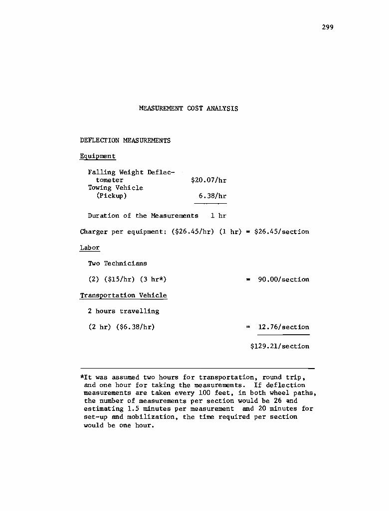
MEASUREMENT COST ANALYSIS
DEFLECTION MEASUREMENTS
Equipment
Falling Weight Deflectometer
Towing Vehicle (Pickup)
$20.07/hr
6.38/hr
Duration of the Measurements 1 hr
Charger per equipment: ($26.45/hr) (1 hr) = $26.45/section
Labor
Two Technicians
(2) ($15/hr) (3 hr*) = 90.00/section
Transportation Vehicle
2 hours travelling
(2 hr) ($6.38/hr) = 12.76/ section
$129. 21/section
*It was assumed two hours for transportation, round trip, and one hour for taking the measurements. If deflection measurements are taken every 100 feet, in both wheel paths, the number of measurements per section would be 26 ~nd estimating 1.5 minutes per measurement and 20 minutes for set-up and mobilization, the time required per section would be one hour.
299

300
MEASUREMENTS COST ANALYSIS
LAYER THICKNESS MEASUREMENTS
Equipment
Not Considered
Labor
Assuming that two test pits 3 ft x 3 ft x 8 in. would be dug, taking 2 hours to perform this, adding two hours for transportation, the charge per job would be, considering two technicians.
(2) ($l5/hr) (4 hr) =
Transportation Vehicle
Travelling: (2 hr) ($6.56 hr) = $13.12
Idle (2 hr) ($2.60/hr) = 5.20
$18.32
Charge for Transportation
Total
$120.00/section
$ 18.32/section
$138. 32/section

MEASUREMENTS COST ANALYSIS
TRAFFIC MEASUREMENTS QUANTIFICATION AND CLASSIFICATION OF THE TRAFFIC
Equipment
Time Lapse Camera $22.48/scction
Time Lapse Projector 1.20/section
$23. 68/section
Charge for Equipment
Labor
Shooting. One technician during seven days for two and a half hours a day:
(7 days) (2.5 hr/day) ($15/hr) = $262.50
Analyzing the film. It will take one technician one hour: (1 hr) ($15/hr) 15.00
$292.50
Charge fo:r Labor
Transportation Vehicle
Travelling: (2 hr/day) (7 days) ($6.56 hr) = $ 91.84
Idle (0.5 hr/day) (7 days) ($2.60 hr) = 9.10
$100.94
$ 23.68/section
$292.50/section
Charge for Tr ansporta tior.. $100.94/ se ct ion
Materials
Super-8 Film
(7 rolls) ($5.60*/each) = $ 39.20
Developing
(7 rolls) ($3.40*/each) = $ 23.80
$ 63.00 (Continued)
301

302
QUANTIFICATION AND CLASSIFICATION OF THE TRAFFIC (Continued)
Materials (Continued)
Other materials such as batteries mounting material, etc., assuming a 10% of the film cost:
(0.10) ($63.00) $ 6.30
$69.30
Charge for Materials:
Total
$ 69.30/section
$486.42/section
An average daily traffic of 60 vpd is assumed. Each vehicle would be filmed for 1.5 minutes. This would represent 90 minutes of film per day. If the picture is shot at 30 frames/minute, 2700 frames would be required. A common super-8 roll has 3600 frames.
*Prices as provided by The University Co-op, Camera Department, Austin, Texas, October 1980.

MEASUREMENT COST ANALYSIS
TRAFFI C MEASUREMENTS AXLE lOADS
Equipment
2 Portable Wheel-load Weighers
(2 units) ($19.75/section)
Labor
2 Technicians surveying for 16 hours per day during the seven days of a week:
= $ 39.,50/ section
(2) ($15.00/hr) (7 days) (16 hr/day) = $3,360.00/section
Transportation Vehicle and Shelter
A mobile home may be provided for this purpose at a charge of $25./day:
(7 days) ($25.00/day) = $ 175.00/section
$3,574.50/section
303

30{J
Equipment Cost Analysis
Rut Depth Gauge
Acquisition cost: $ 400.00 Life (years): 3 Salvage Value: 0%
Ownership cost
Depreciation (D):
D (400.00 - 0.00)/3 years
Investment, insurance, and storage cost (I):
=
I = (400.00 + 0.00)(0.15)/2 =
Maintenance and repairs (M):
M = (133.33)(0.60) =
Total ownership cost:
Operation Cost
Fuel, lubricating oil, etc.
Total operation cost:
Total cost:
$ 133. 33/year
$ 30. DO/year
SO.OO/year
$ 243. 33/year
$ O.OO/year
$ O.DD/year
$ 243.33/year
If one rut depth gauge is used for five sections, and measurements are taken every three weeks, the cost per section would be
Cost per measurement and per section: (243.33)/(5)(18) = $2.70

Equipment Cost Analysis
Transportation vehicle. Pick-up truck, 8 cylinders. Acqusition Cost; $ 6,000 Life (years): 5 Salvage value: 10% Operation hours per year: 1,000
Ownership Cost
Depreciation (D):
D = (6,000 - 600)/(5)(1000) =
Investment, insurance and storage (I): I (6,000 + 600)(0.15)/(2)(1000) =
Maintenace and Repairs (M):
M = (0.50)(1.08) = Total Ownership cost:
Operation Cost
Gasoline: (0.06) (100 HP) (0.60) ( $ 1.1/ga1) =
Oil: [({100 HP)(O.6)(0.006)/7.4) + 4 ga1/100 hour][$ 2/ga1] =
Tires: (4)($ 150.00/each)/2000 hours Total Operation Cost:
Total Cost:
$
$
$
$
$
305
1.08/hour
0.50/hour
0.54/hour
2.12/hour
3.96/hour
0.18/hour 0.18/hour
0.30/hour 4.44/hour
6. 56/hour

306
Equipment Cost Analysis
Mays Meter Unit furnished with DMI and electronic output system Acquisition cost: $ 2,900 Life (years): 3 Salvage value: 20%
Ownership Cost:
Depreciation (D):
D (2,900 - 580)/3 years
Investment, insurance and storage (I):
I = (2,900 + 580)(0.15)/2 =
Maintenance and repairs:
M (0.80) ($ 773.33) =
Operation Cost
Total Cost: $
$ 773. 33/year
261. OO/year
6l8.66/year
O.OO/year
l,652.99/year
If the Mays Meter is calibrated four times during the year, each time requiring three days, the Mays Meter would be available fifty weeks during the year. If measurements are taken every three weeks and if each unit is shared by five sections, the cost per measurement and per section (OMS) would be
CMS = ($ 1,652.99)/(5 sect.) (17 meas./year) $19.45

307
Equipment Cost Analysis
Nuclear Gauge Nuclear Density Meter Mod. NIC-5DT, manufacturd by Soi1test, Inc. Acquisition cost: $ 2,800 Life(years): 4 Salvage value: 0%
Ownership Cost
Depreciation (D):
D = ($ 2800 - 0)/4 years = $ 700.00/year
Investment, insurance and storage (I):
I = (2800 + 0)(6.15)/2 = 210.00/year
Maintenance and Repairs (M):
M * (0.8)($ 700.00) = 560.00/year
Operation Cost O.OO/year
Total Cost: $ 1,470.00/year
Assuming that this device would be shared by five sections and that it would be used for density and moisture measurements every three weeks. The total number of tests that would be performed would be 36 for each of them and the charge for equipment per test (CET) would be
CET = ($ 1,470.00/year)/(5 sect)(36) $ 8.17

308
Equipment Cost Analysis
Mays Meter Automobile Medium size vehicle, six cylinders, gasoline engine Acquisition cost: $ 5,000 Life (years): 4 Salvage Value: 10% Hours per year: 1,000
Ownership Cost
Depreciation (D):
D = (5,000 - 500)/(4)(1,000 hours) =
Investment, insurance and storage (I):
I = (5,000 + 500)(0.15)/(2)(1,000) =
Maintenance and repairs (M):
M = (1.2)($ 1.13) = Total Ownership Cost:
Operation Cost:
$
$
Gasoline: (0.6) (80 HP) (0. 6) ($ lolO/gal) = $
Oil: [«80 HP)(0.6) (0.006)/7.4) + 2 gal/100 hr)][$ 2/gal]=
Tires: (4)($ 100/each)/2000 hr =
Total Operation Cost: $
Total Cost: $
1.13/hour
0.4l/hour
1.35/hour
2.89/hour
3.17 /hoi.lr
O.12/hour
0.20/hour
3.49/hour
6. 38/hour

Equipment Cost Analysis
Falling Weight Def1ectometer Acquisition Cost: $ 60,000 Life (years): 5 Salvage Value: 10% Hours of operation per year: 1,000
Ownership Cost
Depreciation (D):
D = (60,000 - 6,000)/(5)(1,000)
Investment, insurance and storage (I):
I = (60,000 + 6,000)(0.15)/(2)(1,000)
Maintenance and Repairs (M):
M = (0.40)($ 10.80)
Operation Cost
Total Cost:
304}
$ 10.80/hour
4. 95/hour
= 4.32/hour
= O.OO/hour
$ 20.07/hour

310
Equipment Cost Analysis
Portable Wheel Load Weigher Model MD-SOO as manufactured by General E1ectrodinamics Corp., Garland, Tx.; 20,000 1bs capa~ity. Acquisition Cost: $ 1,312.50 Life (years): 3 Salvage value: 0%
Ownership Cost
Depreciation (D) :
D = (1312.50 -0.00)/3 years = $ 437.50/year
Investment, insurance, and storage (I):
I = (1312.50 + 0.00)(0.15)/2 = 98. 44/year
Maintenance and repairs (M):
M = (0.40)($ 437.50) 175.00/year
O£eration Cost = O.OO/year
Total Cost: $ 710. 94/year
Assuming that the axle load measurements would be made once a year, and that the survey would take one week per section, monitoring three sections per month. The charge per section and per survey (CSS) would be
CSS = ($ 710.94)/(12 months) (3) = $ 19.75

311
Equipment Cost Analysis
Time Lapse Camera Model 1240 as distributed including super-8 camera, Acquisition Cost: $
by Timelapse Inc., Mountain View, CA, lenses, iripod, and remote control. 2,075.00
Life (years): Salvage value:
Ownership Cost
Depreciation (D):
4 20%
D = (2075 - 415)/4 years
Investment, insurance, and storage (I):
I = (2075 + 415)(0.15)/2
Maintenance and repairs (M):
M = (0.50)(415.00)
Operation Cost
Total Cost
= $ 4l5.00/year
= 186. 75/year
= 207.50/year
= O.OO/year
$ 809. 25/year
Assuming this camera would be shared by nine sections, making four measurements in each section during the year, the charge for each section and for each measurement (CSM) would be
CSM ($ 809.25)/(9 sect) (4) $ 22.48
* Timelapse price list as June 1980

312
Equipment Cost Analysis
Time Lapse Projector Model 3240 as distributed by Timelapse Inc., Mountain View, CA. Acquisition Cost: $ 2,075 Life (years): 6 Salvage value: 20%
Ownership Cost
Depreciation (D):
D (2075 -415)/6 years $ 276. 67/year
Investment, insurance, and storage (I):
I = (2075 + 415)(0.15)/2 = 186. 75/year
Maintenance and repairs (M):
M (0.50)($ 276.67) = 138. 33/year
Operation Cost = O.OO/year
Total Cost: $ 601. 75/year
Assuming that by using one projector the traffic information from 500 sections may be counted and classified, the charge per section CS would be
CS ($ 601. 75) /500 $ 1. 20

183-8
183-9
183·10
183-11
183-12 184-1
184-2
184-3
184-4F
188-1 I 88-2F 196-IF
198-IF 209-IF
212-IF 244-1 24S-IF SI4-IF 1053-IF
RR 16
RR35
RR36
RR37
RR 38
RR39
RR40 RR43
RR4S RR46
RR41 RR48 RR49 RR50 RR51 RR52 RR53 RRS4 RR55 RR56
,RR60
RR61
RR62 RR63 RR64
(Continuedfrom insidefront cover)
"The Resilient and Fatigue Characteristics of Asphalt Mixtures Processed by the Dryer-Drum Mixer," by Manuel Rodriguez and Thomas W. Kennedy. December 1916. "Fatigue and Repeated-Load Elastic Characteristics of Inservice Portland Cement Concrete," by John A. Crumley and Thomas W. Kennedy. June 1917. "Development of a Mixture Design Procedure for Recycled Asphalt Mixtures." by Ignacio Perez, Thomas W, Kennedy, and Adedare S, Adedimila, November 1918. "An Evaluation of the Texas Blackbase Mix Design Procedure Using the Indirect Tensile Test," by David B, Peters and Thomas W Kennedy, March 1979. "The Effects of Soil Binder and Moisture on Blackbase Mixtures," by Wei-Chou V. Ping and Thomas W. Kennedy, May 1919, "The TEXAS Model for Intersection Traffic-Development," by Clyde E. Lee, Thomas W. Rioux, and Charlie R. Copeland, December 1911. "The TEXAS Model for Intersection Traffic Programmer's Guide," by Clyde E, Lee, Thomas W. Rioux, Vivek S. Savur, and Charlie R. Copeland, December 1917. "The TEXAS Model for Intersection Traffic-User's Guide," by Clyde E. Lee, Glenn E. Grayson. Charlie R. Copeland, Jeff W. Miller, Thomas W. Rioux, and Vivek S. Savur, July 1911. "Application of the TEXAS Model for Analysis of Intersection Capacity and Evaluation of Traffic Control Warrants," by Clyde E. Lee, Vivek S. Savur, and Glenn E. Grayson, July 1918. "Behavior of Stage-Cast Inverted T-Beams with the Precast Flange in Tension," by S. A. A. Wahidi and R. W. Furlong, August 1976. "Strength and Behavior of Stage-Cast Inverted T-Beams," by Richard W Furlong, August 1978. "Design of Reinforcement for Notched Ends of Prestressed Concrete Girders," by Gangadharan Menon and Richard W. Furlong, August 1971. "Control of Cracking on the Side Faces of Large Reinforced Concrete Beams," by G. C. Frantz and J. E. Breen, September 1918. "Fatigue Loading of Cantilever Sign Structures from Truck Wind Gusts," by Bruce M. Creamer, Karl H. Frank, and Richard E. Klingner, April 1979. "Design Criteria for Median Thrn Lanes," by C. Michael Walton, Thomas W. Horne, and William K. Fung, March 1918. "Analysis of Single Piles Under Lateral Loading," by Barry J. Meyer and Lymon C. Reese, December 1979. "Texas Traffic Data Acquisition Program," by Han-Jei Lin, Clyde E. Lee, and Randy Machemehl, February 1980. "Effects of Temperature Change on Plastic Crash Cushions," by Victor N. Toth and Clyde E. Lee, January 1976. "Social Service Agency Transportation Services: Current Operations and the Potential for the Increased Involvement of the Taxi Industry," by Walter L. Cox and Sandra Rosenbloom, August 1917. "The Prediction of Passenger Riding Comfort from Acceleration Data," by Craig C. Smith, David Y. McGehee, and Anthony J. Healey. March 1976. "Perceived Environmental Utility Under Alternative Transportation Systems: A Framework for Analysis," by Pat Burnett, March 1976. "Monitoring the Effects of the Dallas/Fort Worth Regional Airport Volume I: Ground Transportation Impacts," by William 1. Dunlay, Jr., Lyndon Henry, Thomas G. Caffery, Douglas W. Wiersig, and Waldo A. Zambrano, December 1976. "Monitoring the Effects of the Dallas/Fort Worth Regional Airport Volume II: Land Use and Travel Behavior," by Pat Burnett, David Chang, Carl Gregory, Arthur Friedman, Jose Montemayor, and Donna PrestWOOd, July 1976. "The Influence on Rural Communities of Interurban Transportation Systems, Volume II: Transportation and Community Development: A Manual for Small Communities," by C. Michael Walton, John Huddleston, Richard Dodge, Charles Heimsath, Ron Linehan. and John Betak, August 1977. "An Evaluation of Promotional Tactics and Utility Measurement Methods for Public Transportation Systems," by Mark Alpert, Linda Golden, John Betak, James Story, and C. Shane Davies, March \977. "A Survey of Longitudinal Acceleration Comfort Studies in Ground Transportation Vehicles," by L. L. Hoberock, July 1976. "A Pavement Design and Management System for Forest Service Roads - A Working Model," by Freddy L. Roberts, B. Frank McCullough, Hugh J. Williamson, and William R. Wallin, February 1977. "Characteristics of Local Passenger Transportation Providers in Texas," by Ronald Briggs, January 1977. "The Influence on Rural Communities of Interurban 1l'ansportation Systems, Volume I: The Influence on Rural Communities of Interurban Transportation Systems," by C. Michael Walton, Richard Dodge, John Huddleston, John Betak, Ron Linehan, and Charles Heimsath, August 1917. "Effects of Visual Distraction on Reaction Time in a Simulated Traffic Environment," by C. Josh Holahan, March 1977. "Personality Factors in Accident Causation," by Deborah Valentine, Martha Williams, and Robert K. Young, March 1977. "Alcohol and Accidents," by Robert K. Young, Deborah Valentine, and Martha S. Williams, March 1917. "Alcohol Countermeasures," by Gary D. Hales, Martha S. Williams, and Robert K. Young, July 1917. "Drugs and Their Effect on Driving Performance," by Deborah Valentine, Martha S. Williams, and Robert K. Young, May 1977. "Seat Belts: Safety Ignored," by Gary D. Hales, Robert K. Young, and Martha S. Wmiams, June 1978. "Age-Related Factors in Driving Safety," by Deborah Valentine, Martha Williams, and Robert K. Young, February 1978. "Relationships Between Roadside Signs and Traffic Accidents: A Field Investigation," by Charles J. Holahan, November 1977. "Demographic Variables and Accidents," by Deborah Valentine, Martha Williams, and Robert K. Young, January 1978. "Feasibility of Multidisciplinary Accident Investigation in Texas," by Hal L. Fitzpatrick, Craig C. Smith, and Walter S. Reed, September 1977. "A Pavement Design and Management System for Forest Service Roads - Implementation," by B. Frank McCullough and David R. Luhr, January 1979. "Multidisciplinary Accident Investigation," by Deborah Valentine, Gary D, Hales. Martha S. Williams, and Robert K. Young, October 1918. "Psychological Analysis of Degree of Safety in Traffic Environment Design," by Charles J, Holahan, February 1979. "Automobile Collision Reconstruction: A Literature Survey," by Barry D. Olson and Craig C. Smith, December 1979. "An Evaluation of the Utilization of Psychological Knowledge Concerning Potential Roadside Distractors," by Charles J. Holahan. December 1979.

.J CENTEJ:! FOR TRANSPORTATION RESEARCH UBRARY L.:
I IIlfllll III ~I~ 1111I IIIIIIIII~IIIIIIII [039397