A cost function for similarity-based hierarchical clustering

Sanjoy DasguptaUniversity of California, San Diego

dasgupta@eng.ucsd.edu

March 4, 2016

Abstract

The development of algorithms for hierarchical clustering has been hampered by a shortage of preciseobjective functions. To help address this situation, we introduce a simple cost function on hierarchiesover a set of points, given pairwise similarities between those points. We show that this criterion behavessensibly in canonical instances and that it admits a top-down construction procedure with a provablygood approximation ratio.

1 Introduction

A hierarchical clustering is a recursive partitioning of a data set into successively smaller clusters. It isrepresented by a rooted tree whose leaves correspond to the data points, and each of whose internal nodesrepresents the cluster of its descendant leaves.

A hierarchy of this sort has several advantages over a flat clustering, which is a partition of the data intoa fixed number of clusters. First, there is no need to specify the number of clusters in advance. Second, theoutput captures cluster structure at all levels of granularity, simultaneously.

There are several well-established methods for hierarchical clustering, the most prominent among whichare probably the bottom-up agglomerative methods: single linkage, average linkage, and complete linkage(see, for instance, Chapter 14 of [9]). These are widely used and are part of standard packages for dataanalysis. Despite this, there remains an aura of mystery about the kinds of clusters that they find. In part,this is because they are specified procedurally rather than in terms of the objective functions they are tryingto optimize. For many hierarchical clustering algorithms, it is hard to imagine what the objective functionmight be.

This is unfortunate, because the use of objective functions has greatly streamlined the development ofother kinds of data analysis, such as classification methods. Once a cost function is specified, the problemdefinition becomes precise, and it becomes possible to study computational complexity and to compare theefficacy of different proposed algorithms. Also, in practice prior information and other requirements oftenneed to be accommodated, and there is now a well-weathered machinery for incorporating these within costfunctions, as explicit constraints or as regularization terms.

In this work we introduce a simple cost function for hierarchical clustering: a function that, given pairwisesimilarities between data points, assigns a score to any possible tree on those points. Through a series oflemmas (Section 2), we build up intuitions about the kinds of hierarchies that this function favors. Itsbehavior on some canonical examples—points on a line, complete graphs, and planted partitions—can becharacterized readily (Section 3), and corresponds to what one would intuitively want in these cases. Thecost function turns out to be NP-hard to optimize (Section 4), a fate it shares with all the common costfunctions for flat clustering. However, it has a provably-good approximation algorithm (Section 5): a simpletop-down heuristic, variants of which are used in practice for graph partitioning.

1

Related work

Much of the development of hierarchical clustering has taken place within the context of phylogenetics [19,10, 7]. Several of the methods originating in this field, such as average linkage, have subsequently beenadapted for more general-purpose data analysis. This literature has also seen a progression of cost functionsover taxonomies. One of the earliest of these is parsimony: given a collection of vectors x1, . . . , xn ∈ 0, 1p,the idea is to find a tree whose leaves correspond to the xi’s and whose internal nodes are also marked withvectors from the same space, so that total change along the branches of the tree (measured by Hammingdistance, say) is minimized. Later work has moved towards probabilistic modeling, in which a tree defines aprobability space over observable data and the goal is to find the maximum likelihood tree. This is similar inflavor to parsimony, but facilitates the addition of latent variables such as differential rates of mutation alongdifferent branches. Finally, there is the fully Bayesian setting in which a prior is placed over all possible treesand the object is to sample from the posterior distribution given the observations. Although some of theprobabilistic models have been used for more general data (for instance, [17]), they tend to be fairly complexand often implicitly embody constraints—such as a “molecular clock”, in which all leaves are expected tobe roughly equidistant from the root—that are questionable outside the biological context. A more basicand interesting question is to find variants of parsimony that behave reasonably in general settings and thatadmit good algorithms. This is not the agenda of the present paper, however. For instance, our cost functiondoes not assume that the data lie in any particular space, but is based purely on pairwise similarities betweenpoints.

The literature on hierarchical clustering also spans many other disciplines, and there are at least twoother prominent strains of work addressing some of the same concerns that have motivated our search for acost function.

One of these has to do with the statistical consistency of hierarchical clustering methods, as pioneeredby Hartigan [8]. The aim here is to establish that if data is sampled from a fixed underlying distribution,then the tree structure obtained from the data converges in some suitable sense as the sample size grows toinfinity. Only a few methods have been shown to be consistent—single linkage in one dimension, and somevariants of it in higher dimension [4, 6]—and it is an open question to assess the convergence properties, ifany, of other common methods such as average linkage.

Finally, there has been an effort to evaluate hierarchies in terms of cost functions for flat clustering—byevaluating the k-means cost, for example, of a hierarchy truncated to k clusters. Results of this kind areavailable for several standard clustering objectives, including k-center, k-median, and k-means [3, 5, 18, 14].In the present paper, we take a different approach, treating the hierarchies themselves as first-class objectsto be optimized.

On the algorithmic front, the method we ultimately present (Section 5) uses a recursive splitting strategythat is standard in multiway graph partitioning: divide the data into two clusters, then recurse [12]. Thespecific splitting criterion is to find an approximate sparsest cut (by spectral methods, for instance), whichis somewhat surprising because our cost function includes no ratios of any sort. Recursive spectral partition-ing has previously been justified for flat clustering by appealing directly to the conductance of individualclusters [11], whereas in our setting, the same method is seen to produce a hierarchy that approximatelyoptimizes a natural cost function over trees.

2 The cost function and its basic properties

We assume that the input to the clustering procedure consists of pairwise similarities between n data points.Although it would perhaps be most natural to receive this information in matrix form, we will imagine thatit is presented as a weighted graph, as this will facilitate the discussion. The input, then, is an undirectedgraph G = (V,E,w), with one node for each point, edges between pairs of similar points, and positive edgeweights w(e) that capture the degree of similarity. We will sometimes omit w, in which case all edges aretaken to have unit weight.

We would like to hierarchically cluster the n points in a way that is mindful of the given similarity

2

T [u]

u

i j

i _ j

Figure 1: Induced subtrees and least common ancestors.

1

2 4

3

1 23 4

G T5

6 5 6

Figure 2: A small graph G and a candidate hierarchical clustering.

structure. To this end, we define a cost function on possible hierarchies. This requires a little terminology.Let T be any rooted, not necessarily binary, tree whose leaves are in one-to-one correspondence with V . Forany node u of T , let T [u] be the subtree rooted at u, and let leaves(T [u]) ⊆ V denote the leaves of thissubtree. For leaves i, j ∈ V , the expression i ∨ j denotes their lowest common ancestor in T . Equivalently,T [i ∨ j] is the smallest subtree whose leaves include both i and j (Figure 1).

The edges i, j in G, and their strengths wij , reflect locality. When clustering, we would like to avoidcutting too many edges. But in a hierarchical clustering, all edges do eventually get cut. All we can ask,therefore, is that edges be cut as far down the tree as possible. Accordingly, we define the cost of T to be

costG(T ) =∑i,j∈E

wij |leaves(T [i ∨ j])|.

(Often, we will omit the subscript G.) If an edge i, j of unit weight is cut all the way at the top of thetree, it incurs a penalty of n. If it is cut further down, in a subtree that contains α fraction of the data, thenit incurs a smaller penalty of αn.

Figure 2 shows a toy example. Edge 3, 5 is cut at the root of T and incurs a cost of 6. Edges1, 2, 2, 3, 3, 4 each incur a cost of 4, and the remaining three edges cost 1 apiece. Thus costG(T ) =6 + 3× 4 + 3× 1 = 21.

2.1 Two interpretations of the cost function

A natural interpretation of the cost function is in terms of cuts. Each internal node of the tree correspondsto a split in which some subset of nodes S ⊆ V is partitioned into two or more pieces. For a binary split

3

S → (S1, S2), the splitting cost is |S|w(S1, S2), where w(S1, S2) is the weight of the cut,

w(S1, S2) =∑

i,j∈E: i∈S1,j∈S2

wij .

In the example of Figure 2, the top split, 1, 2, 3, 4, 5, 6 → (1, 2, 3, 4, 5, 6) costs 6, while the subsequentsplit 1, 2, 3, 4 → (1, 3, 2, 4) costs 12.

This extends in the obvious way to k-ary splits S → (S1, S2, . . . , Sk), whose cost is |S|w(S1, . . . , Sk), with

w(S1, . . . , Sk) =∑

1≤i<j≤kw(Si, Sj).

The cost of a tree T is then the sum, over all internal nodes, of the splitting costs at those nodes:

cost(T ) =∑

splits S → (S1, . . . , Sk) in T

|S|w(S1, . . . , Sk). (1)

We would like to find the hierarchy T that minimizes this cost.Alternatively, we can interpret a tree T as defining a distance function on points V as follows:

dT (i, j) = |leaves(T [i ∨ j])| − 1.

This is an ultrametric, that is, dT (i, j) ≤ max(dT (i, k), dT (j, k)) for all i, j, k ∈ V . The cost function canthen be expressed as

cost(T ) =∑i,j∈E

wijdT (i, j) + constant.

Thus, we seek a tree that minimizes the average distance between similar points.

2.2 Modularity of cost

An operation we will frequently perform in the course of analysis is to replace a subtree of a hierarchical clus-tering T by some other subtree. The overall change in cost has a simple expression that follows immediatelyfrom the sum-of-splits formulation of equation (1).

Lemma 1 Within any tree T , pick an internal node u. Suppose we obtain a different tree T ′ by replacingT [u] by some other subtree T ′u with the same set of leaves. Then

cost(T ′) = cost(T )− cost(T [u]) + cost(T ′u),

where the costs of T [u] and T ′u are with respect to the original graph restricted to leaves(T [u]).

2.3 The optimal tree is binary

In the figure below, the tree on the left is at least as costly as that on the right.

T1 T2 T3 Tk· · ·T1 T2

T3

Tk· · ·

It follows that there must always exist an optimal tree that is binary—and thus we henceforth limit attentionto the binary case.

4

2.4 Different connected components must first be split apart

If G has several connected components, we would expect a hierarchical clustering to begin by pulling theseapart. This natural property holds under the cost function we are considering.

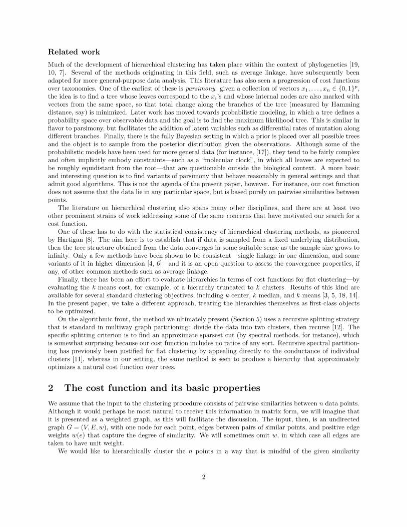
Lemma 2 Suppose an optimal binary tree T contains a subtree T ′ whose leaves induce a subgraph of G thatis not connected. Let the topmost split in T ′ be leaves(T ′)→ (V1, V2). Then w(V1, V2) = 0.

Proof. Suppose, by way of contradiction, that w(V1, V2) > 0. We’ll construct a subtree T ′′ with the sameleaves as T ′ but with lower cost—implying, by modularity of the cost function (Lemma 1), that T cannotbe optimal.

For convenience, write Vo = leaves(T ′), and let U1, U2 be a partition of Vo into two sets that aredisconnected from each other (in the subgraph of G induced by Vo). T ′′ starts by splitting Vo into these twosets, and then copies T ′ on each side of the split.

Vo

U1 U2

T 0

restrictedto U1

T 0

restrictedto U2

T 00 :

The top level of T ′′ has cost zero. Let’s compare level `+ 1 of T ′′ to level ` of T ′. Suppose this level ofT ′ contains some split S → (S1, S2). The cost of this split—its contribution to the cost of T ′—is

cost of split in T ′ = |S|w(S1, S2).

Now, T ′′ has two corresponding splits, S ∩ U1 → (S1 ∩ U1, S2 ∩ U1) and S ∩ U2 → (S1 ∩ U2, S2 ∩ U2). Theircombined cost is

cost of splits in T ′′ = |S ∩ U1|w(S1 ∩ U1, S2 ∩ U1) + |S ∩ U2|w(S1 ∩ U2, S2 ∩ U2)

≤ |S|w(S1 ∩ U1, S2 ∩ U1) + |S|w(S1 ∩ U2, S2 ∩ U2)

= |S|w(S1, S2) = cost of split in T ′,

with strict inequality if S ∩U1 and S ∩U2 are each nonempty and w(S1, S2) > 0. The latter conditions holdfor the very first split of T ′, namely Vo → (V1, V2).

Thus, every level of T ′ is at least as expensive as the corresponding level of T ′′ and the first level isstrictly more expensive, implying cost(T ′′) < cost(T ′), as claimed.

3 Illustrative examples

To get a little more insight into our new cost function, let’s see what it does in three simple and canonicalsituations: the line graph, the complete graph, and random graphs with planted partitions.

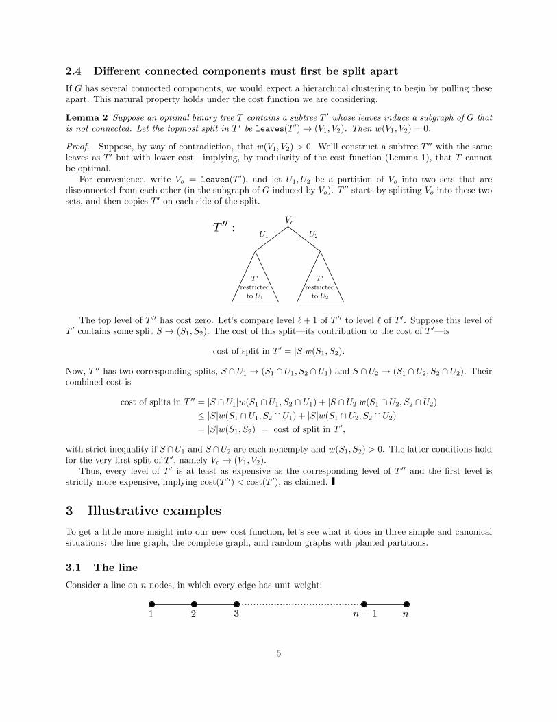
3.1 The line

Consider a line on n nodes, in which every edge has unit weight:

1 2 3 n 1 n

5

A hierarchical clustering need only employ splits consisting of a single edge. This is because any splitthat involves removing multiple edges e1, e2, . . . can be replaced by a series of single-edge splits (first e1,then e2, and so on), with an accompanying reduction in cost.

Let C(n) denote the cost of the best tree for the line on n nodes. The removal of an edge incurs a costof n and creates two smaller versions of the same problem. Thus, for n > 1,

C(n) = n+ min1≤j≤n−1

C(j) + C(n− j).

The best strategy is to split as evenly as possible, into sets of size bn/2c and dn/2e, yielding an overall costC(n) = n log2 n+O(n).

On the other hand, the worst splitting strategy is to choose an extremal edge, which when appliedsuccessively results in a total cost of

n+ (n− 1) + (n− 2) + · · ·+ 2 =n(n+ 1)

2− 1.

3.2 The complete graph

What is the best hierarchical clustering for the complete graph on n nodes, with unit edge weights? It turnsout that all trees have exactly the same cost, which is intuitively pleasing—and will be a crucial tool in ourlater analysis.

Theorem 3 Let G be the complete graph on n nodes, with unit edge weights. For any binary tree T with nleaves,

costG(T ) =1

3(n3 − n).

Proof. For a clique on n nodes, a crude upper bound on the best achievable cost is n ·(n2

), assessing a

charge of n for every edge. We can round this up even further, to n3.Pick any tree T , and uncover it one split at a time, starting at the top. At each stage, we will keep track

of the actual cumulative cost of the splits seen so far, along with a crude upper bound Φ on the cost yet-to-be-incurred. If, for instance, we have uncovered the tree to the point where the bottom nodes correspond tosets of size n1, n2, . . . (summing to n), then the bound on the cost-to-come is Φ = n31 + n32 + · · · .

Initially, we are at the root, have paid nothing yet, and our crude bound on the cost of what lies belowis Φ0 = n3. Let’s say the tth split in the tree, 1 ≤ t ≤ n − 1, breaks a set of size m into sets of size k andm− k. For this split, the immediate cost incurred is ct = mk(m− k) and the crude upper bound on the costyet-to-be-incurred shrinks by

Φt−1 − Φt = m3 − (k3 + (m− k)3) = 3mk(m− k) = 3ct.

When we finally reach the leaves, the remaining cost is zero, but our crude upper bound on it is Φn−1 = n.Thus the total cost incurred is

cost(T ) = c1 + c2 + · · ·+ cn−1 =Φ0 − Φ1

3+

Φ1 − Φ2

3+ · · ·+ Φn−2 − Φn−1

3=

Φ0 − Φn−13

=n3 − n

3,

as claimed.

3.3 Planted partitions

The behavior of clustering algorithms on general inputs is usually quite difficult to characterize. As a result,a common form of analysis is to focus upon instances with “planted” clusters.

The simplest such model, which we shall call the (n, p, q)-planted partition (for an even integer n and0 ≤ q < p ≤ 1), assumes that there are two clusters, each containing n/2 points, and that the neighborhood

6

graph G = (V = [n], E) is constructed according to a generative process. For any pair of distinct nodes i, j,an edge is placed between them with probability

p if i, j are in the same clusterq otherwise

and these(n2

)decisions are made independently. All edges in E are then assigned unit weight. It has been

found, for instance, that spectral methods can recover such partitions for suitable settings of p and q [2, 16].We will also consider what we call the general planted partition model, which allows for an arbitrary

number of clusters C1, C2, . . . , Ck, of possibly different sizes, and has a less constrained generative process.For any pair i, j, the probability that there is an edge between i and j is

> q if i, j are in the same clusterq otherwise

and these decisions need not be independent. Once again, the edges have unit weight.

3.3.1 The general planted partition model

Fix any set of points V = [n], with unknown underlying clusters C1, . . . , Ck. Because the neighborhoodgraph G is stochastic, we will look at the expected cost function,

E[costG(T )] =∑i,j

EG[wij ] |leaves(T [i ∨ j])|

=∑i,j

Pr(edge between i and j in G) |leaves(T [i ∨ j])|.

Lemma 4 For a general planted partition model with clusters C1, . . . , Ck, define graph H = (V, F,w) tohave edges between points in the same cluster, with weights

w(i, j) = Pr(edge between i and j)− q > 0.

In particular, H has k connected components corresponding to the clusters.Now fix any binary tree T with leaves V . For G generated stochastically according to the partition model,

E[costG(T )] =1

3q(n3 − n) + costH(T ).

Proof. Letting Kn denote the complete graph on n nodes (with unit edge weights), we have

E[costG(T )] =∑i,j

Pr(edge between i and j in G) |leaves(T [i ∨ j])|

= q∑i,j|leaves(T [i ∨ j])|+

∑i,j

(Pr(edge between i and j in G)− q) |leaves(T [i ∨ j])|

= q∑i,j|leaves(T [i ∨ j])|+

∑i,j∈F

w(i, j) |leaves(T [i ∨ j])|

= q costKn(T ) + costH(T ).

We then invoke Theorem 3.

Recall that the graph H of Lemma 4 has exactly k connected components corresponding to the underlyingclusters C1, . . . , Ck. By Lemma 2, any tree that minimizes costH(T ), and thus E[costG(T )], must first pullthese components apart.

7

Corollary 5 Pick any binary tree T with leaves V . Under the general planted partition model, T is aminimizer of E[costG(·)] if and only if, for each 1 ≤ i ≤ k, T cuts all edges between cluster Ci and V \ Ci

before cutting any edges within Ci.

Thus, in expectation, the cost function behaves in a desirable manner for data from a planted partition.It is also interesting to consider what happens when sampling error is taken into account. This requiressomewhat more intricate calculations, for which we restrict attention to simple planted partitions.

3.3.2 High probability bounds for the simple planted partition model

Suppose graph G = (V = [n], E) is drawn according to an (n, p, q)-planted partition model, as defined at thebeginning of this section. We have seen that a tree T with minimum expected cost E[costG(T )] is one thatbegins with a bipartition into the two planted clusters (call them L and R).

Moving from expectation to reality, we hope that the optimal tree for G will contain an almost-perfectsplit into L and R, say with at most an ε fraction of the points misplaced. To this end, for any ε > 0, define atree T (with leaves V ) to be ε-good if it contains a split S → (S1, S2) satisfying the following two properties.

• |S ∩ L| ≥ (1− ε)n/2 and |S ∩R| ≥ (1− ε)n/2. That is, S contains almost all of L and of R.

• |S1 ∩ L| ≤ εn/2 and |S2 ∩ R| ≤ εn/2 (or with S1, S2 switched). That is, S1 ≈ R and S2 ≈ L, or theother way round.

As we will see, a tree that is not ε-good has expected cost quite a bit larger than that of optimal trees and,for ε ≈ ((log n)/n)1/2, this difference overwhelms fluctuations due to variance in G.

To begin with, recall from Lemma 4 that when G is drawn from the planted partition model, the expectedcost of a tree T is

E[costG(T )] =1

3q(n3 − n) + (p− q)costH(T ), (2)

where H is a graph consisting of two disjoint cliques of size n/2 each, corresponding to L and R, with edgesof unit weight.

We will also need to consider subgraphs of H. Therefore, define H(`, r) to be a graph with ` + r nodesconsisting of two disjoint cliques of size ` and r. We have already seen (Lemma 2 and Theorem 3) that theoptimal cost for such a graph is

C(`, r)def=

1

3(`3 − `) +

1

3(r3 − r),

and is achieved when the top split is into H(`, 0) and H(0, r). Such a split can be described as laminarbecause it conforms to the natural clusters. We will also consider splits of H(`, 0) or of H(0, r) to be laminar,since these do not cut across different clusters. As we shall now see, any non-laminar split results in increasedcost.

Lemma 6 Consider any hierarchical clustering T of H(`, r) whose top split is into H(`1, r1), H(`2, r2).Then

costH(`,r)(T ) ≥ C(`, r) + `1`2r + r1r2`.

Proof. The top split cuts `1`2 + r1r2 edges. The cost of the two resulting subtrees is at least C(`1, r1) +C(`2, r2). Adding these together,

cost(T ) ≥ (`1`2 + r1r2)(`+ r) + C(`1, r1) + C(`2, r2)

= (`1`2 + r1r2)(`+ r) +1

3

(`31 + `32 − `1 − `2 + r31 + r32 − r1 − r2

)= C(`, r) + `1`2r + r1r2`,

as claimed.

Now let’s return to the planted partition model.

8

Lemma 7 Suppose graph G = (V = [n], E) is generated from the (n, p, q)-planted partition model with p > q.Let T ∗ be a tree whose topmost split divides V into the planted clusters L,R. Meanwhile, let T be a binarytree that is not ε-good, for some 0 < ε < 1/6. Then

E[costG(T )] > E[costG(T ∗)] +1

16ε(p− q)n3.

Proof. Invoking equation (2), we have

E[costG(T )]− E[costG(T ∗)] = (p− q)(costH(n/2,n/2)(T )− costH(n/2,n/2)(T

∗))

= (p− q)(costH(n/2,n/2)(T )− C(n/2, n/2)

).

Thus our goal is to lower-bound the excess cost of T , above the optimal value of C(n/2, n/2), due to thenon-laminarity of its splits. Lemma 6 gives us the excess cost due to any particular split in T , and we will,in general, need to sum this over several splits.

Consider the uppermost node in T whose leaves include at least a (1 − ε) fraction of L as well as of R.Call these points Lo ⊆ L and Ro ⊆ R, and denote the split at this node by

(Lo ∪Ro)→ (L1 ∪R1, L2 ∪R2),

where L1, L2 is a partition of Lo and R1, R2 is a partition of Ro. It helps to think of Lo has having beendivided into a smaller part and a larger part; and likewise with Ro. Since T is not ε-good, it must either bethe case that one of the smaller parts is not small enough, or that the two smaller parts have landed up onthe same side of the split instead of on opposite sides. Formally, one of the two following situations musthold:

1. min(|L1|, |L2|) > εn/2 or min(|R1|, |R2|) > εn/2

2. (|L1| ≤ εn/2 and |R1| ≤ εn/2) or (|L2| ≤ εn/2 and |R2| ≤ εn/2)

In the first case, assume without loss of generality that |L1|, |L2| > εn/2. Then the excess cost due to thenon-laminarity of the split is, from Lemma 6, at least

|L1| · |L2| · |R| >εn

2· (1− 2ε)n

2· (1− ε)n

2

by construction.In the second case, suppose without loss of generality that |L1|, |R1| ≤ εn/2. Since we have chosen the

uppermost node whose leaves include (1− ε) of both L and R, we may also assume |L2| < (1− ε)n/2. Theexcess cost of this non-laminar split and of all other splits S → (S1, S2) on the path up to the root is, againby Lemma 6, at least∑

S→(S1,S2)

|L ∩ S1| · |L ∩ S2| · |R ∩ S| ≥∑

S→(S1,S2)

min(|L ∩ S1|, |L ∩ S2|) ·(1− 2ε)n

2· (1− ε)n

2

>εn

2· (1− 2ε)n

2· (1− ε)n

2,

where the last inequality comes from observing that the smaller portions of each split of L down from theroot have a combined size of exactly |L \ L2| > εn/2.

In either case, we have

costH(n/2,n/2)(T ) > C(n/2, n/2) + ε(1− ε)(1− 2ε)n3

8≥ C(n/2, n/2) +

εn3

16,

which we substitute into our earlier characterization of expected cost.

Thus there is a significant difference in expected cost between an optimal tree and one that is not ε-goodfor large enough ε. We now study the discrepancy between cost(T ) and its expectation.

9

Lemma 8 Let G = (V = [n], E) be a random draw from the (n, p, q)-planted partition model. Then for any0 < δ < 1, with probability at least 1− δ,

maxT|costG(T )− E[costG(T )]| ≤ n2

2

√2n ln 2n+ ln

2

δ,

where the maximum is taken over all binary trees with leaves V .

Proof. Fix any tree T . Then costG(T ) is a function of(n2

)independent random variables (the presence or

absence of each edge); moreover, any one variable can change it by at most n. Therefore, by McDiarmid’sinequality [15], for any t > 0,

Pr(|costG(T )− EcostG(T )| > tn2) ≤ 2 exp

(− 2t2n4(

n2

)n2

)≤ 2e−4t

2

.

Next, we need an upper bound on the number of possible hierarchical clusterings on n points. Imaginereconstructing any given tree T in a bottom-up manner, in a sequence of n− 1 steps, each of which involvesmerging two existing nodes and assigning them a parent. The initial set of points can be numbered 1, . . . , nand new internal nodes can be assigned numbers n+ 1, . . . , 2n− 1 as they arise. Each merger chooses fromat most (2n)2 possibilities, so there are at most (2n)2n possible trees overall.

Taking a union bound over these trees, with 4t2 = ln(2(2n)2n/δ), yields the result.

Putting these pieces together gives a characterization of the tree that minimizes the cost function, fordata from a simple planted partition.

Theorem 9 Suppose G = (V = [n], E) is generated at random from an (n, p, q)-planted partition model. LetT be the binary tree that minimizes costG(·). Then for any δ > 0, with probability at least 1− δ, T is ε-goodfor

ε =16

p− q

√2 ln 2n

n+

1

n2ln

2

δ,

provided this quantity is at most 1/6.

Proof. Let T ∗ be a tree whose top split divides V into its true clusters, and let T be the minimizer ofcostG(·). Since costG(T ) ≤ costG(T ∗), it follows from Lemma 8 that

E[costG(T )] ≤ E[costG(T ∗)] + n2√

2n ln 2n+ ln2

δ.

Now, if T fails to be ε-good for some 0 < ε ≤ 1/6, then by Lemma 7,

ε <16

(p− q)n3 (E[costG(T )]− E[costG(T ∗)]) .

Combining these inequalities yields the theorem statement.

In summary, when data is generated from a simple partition model, the tree that minimizes cost(T )almost perfectly respects the planted clusters, misplacing at most an O(

√(lnn)/n) fraction of the data.

4 Hardness of finding the optimal clustering

In this section, we will see that finding the tree that minimizes the cost function is NP-hard. We begin byconsidering a related problem.

10

4.1 Maximizing the cost function

Interestingly, the problem of maximizing cost(T ) is equivalent to the problem of minimizing it. To see this,let G = (V,E) be any graph with unit edge weights, and let Gc = (V,Ec) denote its complement. Pick anytree T and assess its suitability as a hierarchical clustering of G and also of Gc:

costG(T ) + costGc(T ) =∑i,j∈E

|leaves(T [i ∨ j])|+∑

i,j∈Ec

|leaves(T [i ∨ j])|

=∑i,j|leaves(T [i ∨ j])|

= costKn(T ) =n3 − n

3

where Kn is the complete graph on n nodes, and the last equality is from Theorem 3. In short: a treethat maximizes cost(T ) on G also minimizes cost(T ) on Gc, and vice versa. A similar relation holds inthe presence of edge weights, where the complementary weights wc are chosen so that w(i, j) + wc(i, j) isconstant across all i, j.

In proving hardness, it will be convenient to work with the maximization version.

4.2 A variant of not-all-equal SAT

We will reduce from a special case of not-all-equal SAT that we call NAESAT∗:

NAESAT∗

Input: A Boolean formula in CNF such that each clause has either two or three literals, and eachvariable appears exactly three times: once in a 3-clause and twice, with opposite polarities, in2-clauses.

Question: Is there an assignment to the variables under which every clause has at least onesatisfied literal and one unsatisfied literal?

In a commonly-used version of NAESAT, which we will take to be standard, there are exactly threeliterals per clause but each variable can occur arbitrarily often. Given an instance φ(x1, . . . , xn) of this type,we can create an instance φ′ of NAESAT∗as follows:

• Suppose variable xi occurs k times in φ. Without loss of generality, k > 1 (otherwise we can discardthe containing clause with impunity). Create k new variables xi1, . . . , xik to replace these occurrences.

• Enforce agreement amongst xi1, . . . , xik by adding implications

(xi1 ∨ xi2), (xi2 ∨ xi3), . . . , (xik ∨ xi1).

These k clauses are satisfied ⇐⇒ they are not-all-equal satisfied ⇐⇒ xi1 = xi2 = · · · = xik.

Then φ′ has the required form, and moreover is not-all-equal satisfiable if and only if φ is not-all-equalsatisfiable.

4.3 Hardness of maximizing cost(T )

We now show that it is NP-hard to find a binary tree that maximizes cost(T ).

Theorem 10 Given an instance φ of NAESAT∗, we can in polynomial time specify a weighted graph G =(V,E,w) and integer M such that

• maxe∈E w(e) is polynomial in the size of φ, and

11

• φ is not-all-equal satisfiable if and only if there exists a binary tree T with costG(T ) ≥M .

Proof. Suppose instance φ(x1, . . . , xn) has m clauses of size three and m′ clauses of size two. We willassume that certain redundancies are removed from φ:

• If there exists a 2-clause C whose literals also appear in a 3-clause C ′, then C ′ is redundant and canbe removed.

• The same holds if the 3-clause C ′ contains the two literals of C with polarity reversed. This is because(x ∨ y) is not-all-equal satisfied if and only if (x ∨ y) is not-all-equal satisfied.

• Likewise, if there is a 2-clause C whose literals also appear in a 2-clause C ′, but with reversed polarity,then C ′ can be removed.

• Any clause that contains both a literal and its negation can be removed.

Based on φ, construct a weighted graph G = (V,E,w) with 2n vertices, one per literal (xi and xi). Theedges E fall into three categories:

1. For each 3-clause, add six edges to E: one edge joining each pair of literals, and one edge joining thenegations of those literals. These form two triangles. For instance, the clause (x1 ∨ x2 ∨ x3) becomes:

x1

x3 x2

x1

x2 x3

These edges have weight 1.

2. Similarly, for each 2-clause, add two edges of unit weight: one joining the two literals, and one joiningtheir negations.

3. Finally, add n edges xi, xi of weight W = 2nm+ 1.

Under the definition of NAESAT∗, and with the removal of redundancies, these 6m+ 2m′ + n edges are alldistinct.

Now suppose φ is not-all-equal satisfiable. Let V + ⊂ V be the positive literals under the satisfyingassignment, and V − the negative literals. Consider a two-level tree T :

V

V + V

The top split cuts all edges of G, except for one edge per triangle (and there are 2m of these). The costof this split is

|V | · w(V +, V −) = 2n(4m+ 2m′ + nW ).

12

function MakeTree(V)

If |V | = 1: return leaf containing the singleton element in VLet (S, V \ S) be an αn-approximation to the sparsest cut of VLeftTree = MakeTree(S)RightTree = MakeTree(V \ S)Return [LeftTree, RightTree]

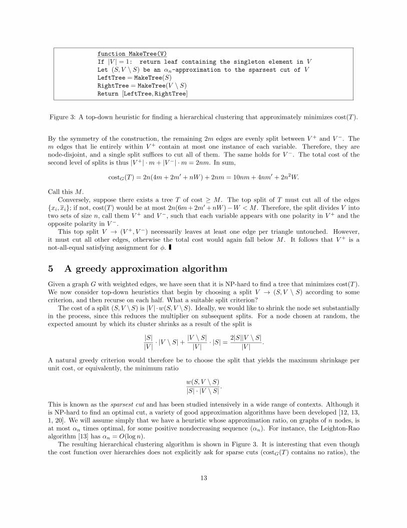
Figure 3: A top-down heuristic for finding a hierarchical clustering that approximately minimizes cost(T ).

By the symmetry of the construction, the remaining 2m edges are evenly split between V + and V −. Them edges that lie entirely within V + contain at most one instance of each variable. Therefore, they arenode-disjoint, and a single split suffices to cut all of them. The same holds for V −. The total cost of thesecond level of splits is thus |V +| ·m+ |V −| ·m = 2nm. In sum,

costG(T ) = 2n(4m+ 2m′ + nW ) + 2nm = 10nm+ 4nm′ + 2n2W.

Call this M .Conversely, suppose there exists a tree T of cost ≥ M . The top split of T must cut all of the edges

xi, xi; if not, cost(T ) would be at most 2n(6m+ 2m′+nW )−W < M . Therefore, the split divides V intotwo sets of size n, call them V + and V −, such that each variable appears with one polarity in V + and theopposite polarity in V −.

This top split V → (V +, V −) necessarily leaves at least one edge per triangle untouched. However,it must cut all other edges, otherwise the total cost would again fall below M . It follows that V + is anot-all-equal satisfying assignment for φ.

5 A greedy approximation algorithm

Given a graph G with weighted edges, we have seen that it is NP-hard to find a tree that minimizes cost(T ).We now consider top-down heuristics that begin by choosing a split V → (S, V \ S) according to somecriterion, and then recurse on each half. What a suitable split criterion?

The cost of a split (S, V \S) is |V | ·w(S, V \S). Ideally, we would like to shrink the node set substantiallyin the process, since this reduces the multiplier on subsequent splits. For a node chosen at random, theexpected amount by which its cluster shrinks as a result of the split is

|S||V | · |V \ S|+

|V \ S||V | · |S| =

2|S||V \ S||V | .

A natural greedy criterion would therefore be to choose the split that yields the maximum shrinkage perunit cost, or equivalently, the minimum ratio

w(S, V \ S)

|S| · |V \ S| .

This is known as the sparsest cut and has been studied intensively in a wide range of contexts. Although itis NP-hard to find an optimal cut, a variety of good approximation algorithms have been developed [12, 13,1, 20]. We will assume simply that we have a heuristic whose approximation ratio, on graphs of n nodes, isat most αn times optimal, for some positive nondecreasing sequence (αn). For instance, the Leighton-Raoalgorithm [13] has αn = O(log n).

The resulting hierarchical clustering algorithm is shown in Figure 3. It is interesting that even thoughthe cost function over hierarchies does not explicitly ask for sparse cuts (costG(T ) contains no ratios), the

13

sparsest cut objective emerges organically when one adopts a greedy top-down approach to constructing thetree.

We will now see that this algorithm returns a tree of cost at most O(αn log n) times optimal. The firststep is to show that if there exists a low cost tree, there must be a correspondingly sparse cut of V .

Lemma 11 Pick any binary tree T on V . There exists a partition A,B of V such that

w(A,B)

|A| · |B| <27

4|V |3 cost(T ),

and for which |V |/3 ≤ |A|, |B| ≤ 2|V |/3.

Proof. The diagram below shows a portion of T , drawn in a particular way. Each node u is labeled withthe leaf set of its induced subtree T [u]. We always depict the smaller half of each cut (Ai, Bi) on the right,so that |Ai| ≥ |Bi|.

A1

A2

Ak Bk

B1

B2

B3

V

Ak1

Let n = |V |. Pick the smallest k so that |B1|+ · · ·+ |Bk| ≥ n/3. This also means |Ak−1| > 2n/3 (to dealwith cases when k = 1, let Ao = V ) and |Ak| > n/3. Define A = Ak and B = B1 ∪ · · · ∪Bk.

Now,

cost(T ) ≥ w(A1, B1) · n+ w(A2, B2) · |A1|+ · · ·+ w(Ak, Bk) · |Ak−1|

>2n

3(w(A1, B1) + · · ·+ w(Ak, Bk))

≥ 2n

3w(A,B)

since the removal of all the edges in the cuts (A1, B1), . . . , (Ak, Bk) disconnects Ak from B1 ∪ · · · ∪ Bk.Therefore,

w(A,B)

|A| · |B| <3

2n· cost(T )

(2n/3) · (n/3)=

27

4n3cost(T ),

as claimed.

Theorem 12 Pick any graph G on n vertices, with positive edge weights w : E → R+. Let tree T ∗ be aminimizer of costG(·) and let T be the tree returned by the top-down algorithm of Figure 3. Then

costG(T ) ≤ (cn lnn)costG(T ∗),

for cn = 27αn/4.

14

Proof. We’ll use induction on n. The case n = 1 is trivial since any tree with one node has zero cost.Assume the statement holds for graphs of up to n− 1 nodes. Now pick a weighted graph G = (V,E,w)

with n nodes, and let T ∗ be an optimal tree for it. By Lemma 11, the sparsest cut of G has ratio at most

27

4n3cost(T ∗).

The top-down algorithm identifies a partition (A,B) of V that is an αn-approximation to this cut, so that

w(A,B)

|A| · |B| ≤27αn

4n3cost(T ∗) =

cnn3

cost(T ∗),

and then recurses on A and B.We now obtain an upper bound on the cost of the best tree for A (and likewise B). Start with T ∗, restrict

all cuts to edges within A, and disregard subtrees that are disjoint from A. The resulting tree, call it T ∗A,has the same overall structure as T ∗. Construct T ∗B similarly. Now, for any split S → (S1, S2) in T ∗ thereare corresponding (possibly empty) splits in T ∗A and T ∗B . Moreover, the cut edges in T ∗A and T ∗B are disjointsubsets of those in T ∗; hence the cost of this particular split in T ∗A and T ∗B combined is at most the cost inT ∗. Formally,

(cost of split in T ∗A) + (cost of split in T ∗B) = |S ∩A| · w(S1 ∩A,S2 ∩A) + |S ∩B| · w(S1 ∩B,S2 ∩B)

≤ |S| · w(S1 ∩A,S2 ∩A) + |S| · w(S1 ∩B,S2 ∩B)

≤ |S| · w(S1, S2) = cost of split in T ∗.

Summing over all splits, we havecost(T ∗A) + cost(T ∗B) ≤ cost(T ∗).

Here the costs on the left-hand side are with respect to the subgraphs of G induced by A and B, respectively.Without loss of generality, |A| = pn and |B| = (1− p)n, for some 0 < p < 1/2. Recall that our algorithm

recursively constructs trees, say TA and TB , for subsets A and B. Applying the inductive hypothesis to thesetrees, we have

cost(TA) ≤ cncost(T ∗A) ln pn

cost(TB) ≤ cncost(T ∗B) ln(1− p)n

where we have used the monotonicity of (αn), and hence

cost(T ) ≤ n · w(A,B) + cost(TA) + cost(TB)

≤ n · |A| · |B| · cnn3· cost(T ∗) + cncost(T ∗A) ln pn+ cncost(T ∗B) ln(1− p)n

≤ cnp(1− p) · cost(T ∗) + cncost(T ∗A) ln(1− p)n+ cncost(T ∗B) ln(1− p)n≤ cnp · cost(T ∗) + cncost(T ∗) ln(1− p)n= cncost(T ∗) (p+ ln(1− p) + lnn)

≤ cncost(T ∗) lnn,

as claimed.

Is this approximation guarantee non-trivial? Recall the example of a line graph (Section 3.1): there, wefound that a good hierarchy has cost O(n log n) while a bad hierarchy has cost Ω(n2). For sparse graphs ofthis kind, a polylogarithmic approximation guarantee is useful. For dense graphs, however, all clusteringshave cost Ω(n3), and thus the guarantee ceases to be meaningful.

15

6 A generalization of the cost function

A more general objective function for hierarchical clustering is

costG(T ) =∑i,j∈E

wij f(|leaves(T [i ∨ j])|),

where f is defined on the nonnegative reals, is strictly increasing, and has f(0) = 0. For instance, we couldtake f(x) = ln(1 + x) or f(x) = x2.

Under this generalized cost function, all the properties of Section 2 continue to hold, substituting |S| byf(|S|) as needed, for S ⊆ V . However, it is no longer the case that for the complete graph, all trees haveequal cost. When G is the clique on four nodes, for instance, the two trees shown below (T1 and T2) neednot have the same cost.

1

3 4

2

1 2 3 4

12

3 4

K4 T1 T2

The tree costs, for any f , are:

cost(T1) = 4f(4) + 2f(2)

cost(T2) = 3f(4) + 2f(3) + f(2)

Thus T1 is preferable if f is concave (in which case f(2) + f(4) ≤ 2f(3)), while the tables are turned if f isconvex.

Nevertheless, the greedy top-down heuristic continues to yield a provably good approximation. It needsto be modified slightly: the split chosen is (an αn-approximation to) the minimizer S ⊆ V of

w(S, V \ S)

min(f(|S|), f(|V \ S|)) subject to1

3|V | ≤ |S| ≤ 2

3|V |.

Lemma 11 and Theorem 12 need slight revision.

Lemma 13 Pick any binary tree T on V . There exists a partition A,B of V such that

w(A,B)

min(f(|A|), f(|B|)) ≤cost(T )

f(b2n/3c)f(dn/3e) .

and for which |V |/3 ≤ |A|, |B| ≤ 2|V |/3.

Proof. Sets A,B are constructed exactly as in the proof of Lemma 11. Then, referring to the diagram inthat proof,

cost(T ) ≥ w(A1, B1) · f(n) + w(A2, B2) · f(|A1|) + · · ·+ w(Ak, Bk) · f(|Ak−1|)≥ f(b2n/3c) (w(A1, B1) + · · ·+ w(Ak, Bk)) ≥ f(b2n/3c)w(A,B),

whereuponw(A,B)

min(f(|A|), f(|B|)) ≤cost(T )

f(b2n/3c)f(dn/3e) .

16

Theorem 14 Pick any graph G on n vertices, with positive edge weights w : E → R+. Let tree T ∗ be aminimizer of cost(·) and let T be the tree returned by the modified top-down algorithm. Then

costG(T ) ≤ (cn lnn) costG(T ∗),

where

cn = 3αn · max1≤n′≤n

f(n′)f(dn′/3e) .

Proof. The proof outline is as before. We assume the statement holds for graphs of up to n− 1 nodes. Nowpick a weighted graph G = (V,E,w) with n nodes, and let T ∗ be an optimal tree for it.

Let T denote the tree returned by the top-down procedure. By Lemma 13, the top split V → (A,B)satisfies n/3 ≤ |A|, |B| ≤ 2n/3 and

w(A,B) ≤ αn min(f(|A|), f(|B|)) cost(T ∗)f(b2n/3c)f(dn/3e) ≤

αn

f(dn/3e)cost(T ∗),

where the last inequality uses the monotonicity of f .As before, the optimal tree T ∗ can be used to construct trees T ∗A and T ∗B for point sets A and B,

respectively, such that cost(T ∗A) + cost(T ∗B) ≤ cost(T ∗). Meanwhile, the top-down algorithm finds trees TAand TB which, by the inductive hypothesis, satisfy

cost(TA) ≤ (cn ln |A|)cost(T ∗A)

cost(TB) ≤ (cn ln |B|)cost(T ∗B)

Let’s say, without loss of generality, that |A| ≤ |B|. Then

cost(T ) ≤ f(n) · w(A,B) + cost(TA) + cost(TB)

≤ f(n) · w(A,B) + (cn ln |B|)(cost(T ∗A) + cost(T ∗B))

≤ αnf(n)

f(dn/3e)cost(T ∗) + (cn lnn+ cn ln(2/3))cost(T ∗)

≤ cn3

cost(T ∗) + (cn lnn− cn/3)cost(T ∗) = (cn lnn)cost(T ∗),

as claimed.

Acknowledgements

The author is grateful to the National Science Foundation for support under grant IIS-1162581.

References

[1] S. Arora, S. Rao, and U.V. Vazirani. Expander flows, geometric embeddings and graph partitioning.Journal of the Association for Computing Machinery, 56(2), 2009.

[2] R.B. Boppana. Eigenvalues and graph bisection: an average-case analysis. In IEEE Symposium onFoundations of Computer Science, pages 280–285, 1985.

[3] M. Charikar, C. Chekuri, T. Feder, and R. Motwani. Incremental clustering and dynamic informationretrieval. SIAM Journal on Computing, 33(6):1417–1440, 2004.

[4] K. Chaudhuri, S. Dasgupta, S. Kpotufe, and U. von Luxburg. Consistent procedures for cluster treeestimation and pruning. IEEE Transactions on Information Theory, 60(12):7900–7912, 2014.

17

[5] S. Dasgupta and P.M. Long. Performance guarantees for hierarchical clustering. Journal of Computerand System Sciences, 70(4):555–569, 2005.

[6] J. Eldridge, M. Belkin, and Y. Wang. Beyond Hartigan consistency: merge distortion metric for hier-archical clustering. In 28th Annual Conference on Learning Theory, 2015.

[7] J. Felsenstein. Inferring Phylogenies. Sinauer, 2004.

[8] J.A. Hartigan. Statistical theory in clustering. Journal of Classification, 2:63–76, 1985.

[9] T. Hastie, R. Tibshirani, and J. Friedman. The Elements of Statistical Learning. Springer, 2nd edition,2009.

[10] N. Jardine and R. Sibson. Mathematical Taxonomy. John Wiley, 1971.

[11] R. Kannan, S. Vempala, and A. Vetta. On clusterings: good, bad, and spectral. Journal of the ACM,51(3):497–515, 2004.

[12] B.W. Kernighan and S. Lin. An efficient heuristic procedure for partitioning graphs. Bell SystemTechnical Journal, 49(2):291–307, 1970.

[13] F.T. Leighton and S. Rao. Multicommodity max-flow min-cut theorems and their use in designingapproximation algorithms. Journal of the Association for Computing Machinery, 46(6):787–832, 1999.

[14] G. Lin, C. Nagarajan, R. Rajaraman, and D.P. Williamson. A general approach for incremental ap-proximation and hierarchical clustering. SIAM Journal on Computing, 39:3633–3669, 2010.

[15] C. McDiarmid. On the method of bounded differences. Surveys in Combinatorics, 141:148–188, 1989.

[16] F. McSherry. Spectral partitioning of random graphs. In IEEE Symposium on Foundations of ComputerScience, pages 529–537, 2001.

[17] R.M. Neal. Density modeling and clustering using Dirichlet diffusion trees. In J.M. Bernardo et al.,editors, Bayesian Statistics 7, pages 619–629. Oxford University Press, 2003.

[18] C.G. Plaxton. Approximation algorithms for hierarchical location problems. Journal of Computer andSystem Sciences, 72:425–443, 2006.

[19] R.R. Sokal and P.H.A. Sneath. Numerical Taxonomy. W.H. Freeman, 1963.

[20] U. von Luxburg. A tutorial on spectral clustering. Statistics and Computing, 17(4):395–416, 2007.

18