a control architecture for a mobile heavy-lift precision manipulator
TRANSCRIPT
A Control Architecture for a Mobile Heavy-Lift Precision Manipulator with Limited
Sensory Information
William Becker, Matthew DiCicco, Justin Garretson and Steven Dubowsky* Mechanical Engineering Field and Space Robotics Laboratory
Massachusetts Institute of Technology Room 3-469, 77 Massachusetts Ave.
Cambridge, MA, 02139, USA
* Corresponding author [email protected]
ABSTRACT
Mobile robotic manipulators can augment the strength and dexterity of human operators in
unstructured environments. Here, the control system for a six degree-of-freedom heavy-lift
mobile manipulator for lifting and inserting payloads on the deck of a ship is described. The
robotic hardware and the application present several control challenges, including structural
resonances, high joint friction that varies with time, limited sensors for measuring the joint
friction, complex interaction with the environment, tight tolerances for the insertion tasks, lack of
bilateral force feedback of the contact forces, and ship motions. The control system enables an
operator to perform insertion tasks using feedback of tactile clues of the manipulator position,
and reduces the effects of friction with a combination of sensor-based, adaptive, and model-
based methods of friction compensation. The control architecture is validated in simulation and
on a laboratory manipulator.
I. INTRODUCTION
Mobile robotic manipulators can be used to augment the strength and dexterity of a human
operator, allowing them to perform otherwise difficult or impossible tasks, often in unstructured,
harsh environments in the presence of substantial environmental disturbances. However, heavy
payloads, tight tolerances, and design constraints can combine to make the control of these
systems difficult.
In this paper, the control of a teleoperated six degree-of-freedom manipulator for lifting very
heavy payloads on the decks of ships and inserting these payloads onto racks with tight
tolerances is studied, see Figure 1. The manipulator is mounted on an omni-directional vehicle
that allows the robot to move from point to point while carrying the payload. The system will
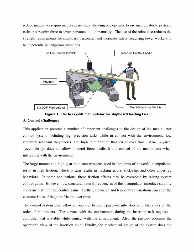
reduce manpower requirements aboard ship, allowing one operator to use manipulator to perform
tasks that require three to seven personnel to do manually. The use of the robot also reduces the
strength requirements for shipboard personnel, and increases safety, requiring fewer workers to
be in potentially dangerous situations.
Figure 1: The heavy-lift manipulator for shipboard loading task. A. Control Challenges
This application presents a number of important challenges to the design of the manipulator
control system, including high-precision tasks while in contact with the environment, low
structural resonant frequencies, and high joint friction that varies over time. Also, physical
system design does not allow bilateral force feedback and control of the manipulator when
interacting with the environment.
The large motors and high gear-ratio transmissions used in the joints of powerful manipulators
result in high friction, which in turn results in tracking errors, stick-slip, and other undesired
behaviors. In some applications, these friction effects may be overcome by raising system
control gains. However, low structural natural frequencies of this manipulator introduce stability
concerns that limit the control gains. Further, corrosion and temperature variations can alter the
characteristics of the joint friction over time.
The control system must allow an operator to insert payloads into slots with tolerances on the
order of millimeters. The contact with the environment during the insertion task requires a
controller that is stable while contact with the environment. Also, the payload obscures the
operator’s view of the insertion point. Finally, the mechanical design of the system does not
Position Control Joystick Insertion Control Handle
Omni-Directional Vehicle
Payload
Six DOF Manipulator

permit the use of a powered master controller that would allow bilateral force feedback of the
contact forces.
The objective of this paper is to develop a control architecture that is able to compensate for the
high joint friction in the manipulator and enable an operator to perform insertion tasks without
bilateral force feedback and limited task view.
B. Background Literature
Many control methods have been suggested to estimate and compensate for the effects of joint
friction [2]. These methods generally fall into three categories: model-based compensation,
adaptive compensation, and sensor-based compensation.
Model-based friction compensation uses mathematical models to predict joint friction, which is
then compensated with motor torque [15,30]. The effectiveness of this type of compensation
depends on the accuracy of the models. Accurate characterization of joint friction is difficult in
harsh environments such as this one, as friction changes over time with variations in temperature
and wear [32].
To compensate for friction variations, methods have been proposed for online estimation of
friction parameters using adaptive and observer-based approaches [2,5,12, 17]. These methods
take advantage of known and measured system dynamics to identify the friction parameters
online. Online friction identification and compensation using single-joint observer methods has
resulted in good position control performance in systems with high joint friction [24,25].
However, single-joint adaptive identification is not practical when the manipulator is in contact
with the environment, because adaptive identification may interpret contact forces as frictional
disturbances. Adaptive friction compensation for systems in contact with the environment
requires an adaptive model-based feed-forward structure, as well as a contact force sensor so the
controller can differentiate between joint friction and contact forces [38]. The formulation of
these adaptive methods is quite complex, especially for high-degree-of-freedom systems [31]. In
the system studied here, direct measurement of the contact forces is not feasible.
Sensor-based compensation overcomes many of the problems of model-based and adaptive
methods, but can only be used when the design of the robot allows the placement of sensors to
provide direct feedback of the system friction. Torque control loops can then be used to reduce
the effects of friction [28,33]. No model of the friction is required and the compensation is
robust to friction changes with wear or temperature. This method has been shown to provide
accurate compensation for joint friction; however, providing sensors at each joint can be costly
and add substantial system complexity. More recently, a sensor-based method has been
proposed that permits the friction in all joints to be estimated using a single six-degree-of-
freedom force/torque sensor in the manipulator’s base, greatly simplifying the hardware
implementation of sensor-based approaches [19,29].
For this system, the manipulator is controlled by a human operator. Teleoperated position
control of a manipulator is well-studied, and relatively straightforward. Approaches such as
Jacobian inverse control with linear joint controllers [3,39], sliding mode control [3,35], and
adaptive control [7,36] are all established means of controlling the position and velocity of a
manipulator. Coordinated vehicle and manipulator control is also well studied [34,40]. In this
system, because of the extremely heavy payloads, stab jacks lift the omni-directional wheels off
of the ground when the manipulator is being controlled by the operator, effectively providing a
base for the manipulator that is fixed to the ship. The use of these stab jacks prevents low
frequency manipulator and suspension vibrations that could lead to system instabilities. Hence,
the manipulator controller does not need to consider vehicle motions, although it must
compensate for the substantial dynamic effects of the ship pitching and rolling in heavy seas.
During payload insertion, when the manipulator is in contact with the environment, it is
important to carefully control the forces exerted by the manipulator to prevent payload jamming.
A number of manipulator force controllers have been proposed, including explicit force control,
hybrid control, and stiffness/impedance control [6,18,37]. When a human is operating a
manipulator under force control, best performance occurs when the operator is able to “feel” the
forces and moments measured by a force/torque sensor close to the contact points, and controls
the robot by applying forces to a force-sensitive input device. This structure is known as
bilateral force feedback, and has been shown to be effective in the control of many teleoperated
systems [1,16]. However, to be effective, the operator interface system must be actively
powered. This adds substantial complexity to the physical and control system, as well as
additional cost. Such a user interface was not considered feasible for this system, as shown in
Figure 1.
In summary, sensor-based methods of friction compensation are preferred when the sensor
hardware is available. Adaptive methods can perform very well, but cannot easily handle contact
forces. Model-based methods are more stable, but are not robust to unmodeled or time-varying
effects. Because the system in this report has low structural natural frequencies, a high-gain
linear controller is not feasible. The system design does not permit force sensors that can
measure all of the joint torques and the forces and moments at the manipulator’s contact with the
environment. Finally, a simple model-based compensator would not be effective because of the
very large changes in the friction over time caused by the harsh ship deck environment, wear,
changing loads, etc.
C. Approach
In this study, a control architecture has been developed that is an amalgam of the above
approaches. In the joints that do not have force sensors, an adaptive algorithm is used when the
manipulator is moving in free space, and data from this algorithm is used update the parameters
in a model-based feed-forward compensation algorithm that is used when the manipulator is in
contact with the environment. This approach compensates for time-varying friction and remains
stable in the presence of contact forces. This friction compensation architecture is validated in
simulations of the full scale manipulator, as well as in experiments with a laboratory robot.
While bilateral force feedback is not possible here because of the lack of a powered master
control interface, the presence of an operator insertion force input handle located on the
manipulator close to the payload allows some tactile feedback by enabling the operator to feel
small motions of the manipulator. This type of robot is referred to as an "extender" or
"exoskeleton" system. A number of control strategies have been proposed for such structures
[8,10,20,21,22,23,26,27]. A variation of these methods are applied here with good results as
shown by laboratory experiments.
II. SYSTEM DESCRIPTION
A. Joint Configuration
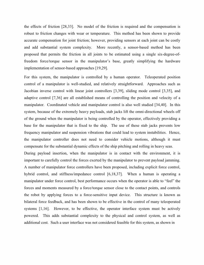
Figure 2 shows the joint configuration and coordinate systems of the manipulator. All the joints
are powered by electric actuators. Joints one and two of the manipulator are base yaw and pitch
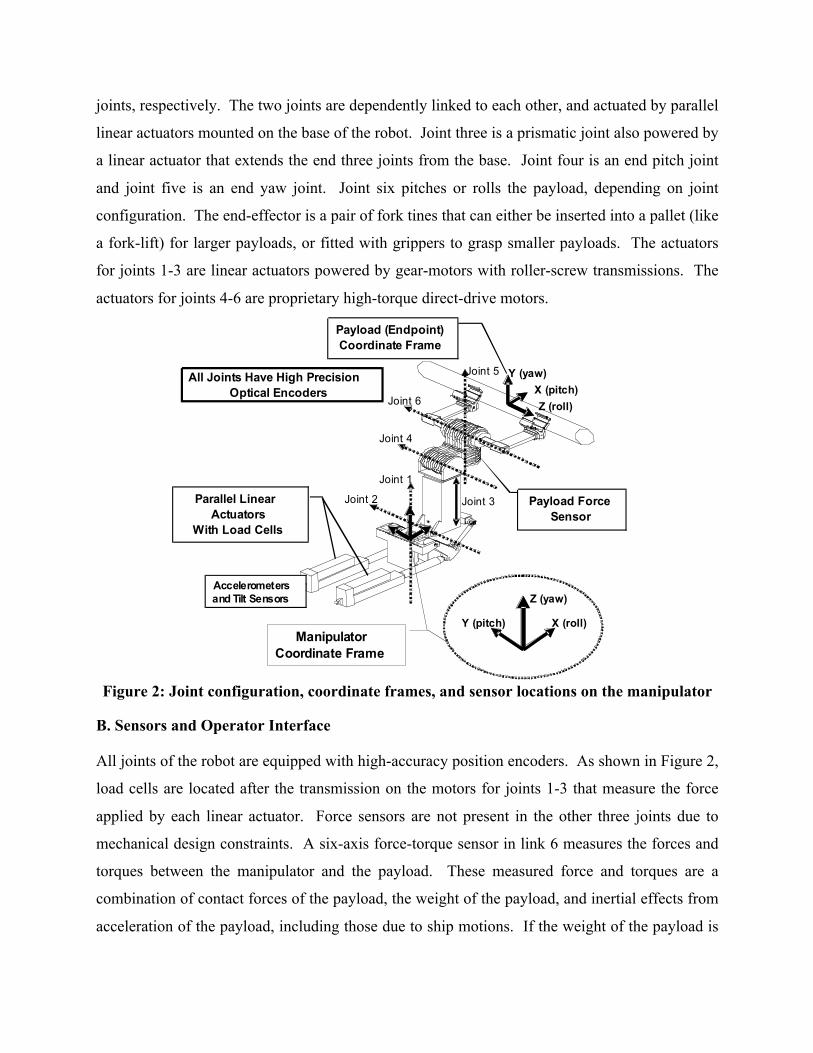
joints, respectively. The two joints are dependently linked to each other, and actuated by parallel
linear actuators mounted on the base of the robot. Joint three is a prismatic joint also powered by
a linear actuator that extends the end three joints from the base. Joint four is an end pitch joint
and joint five is an end yaw joint. Joint six pitches or rolls the payload, depending on joint
configuration. The end-effector is a pair of fork tines that can either be inserted into a pallet (like
a fork-lift) for larger payloads, or fitted with grippers to grasp smaller payloads. The actuators
for joints 1-3 are linear actuators powered by gear-motors with roller-screw transmissions. The
actuators for joints 4-6 are proprietary high-torque direct-drive motors. Kinematic Coordinate Frames
Payload (Endpoint) Coordinate Frame
All Joints Have High Precision Optical Encoders
Parallel Linear Actuators
With Load Cells
Joint 2
Joint 5
Joint 3
Joint 1
Joint 4
Joint 6
Y (pitch) X (roll)
Z (yaw)
Manipulator Coordinate Frame
Y (yaw)X (pitch)Z (roll)
Accelerometersand Tilt Sensors
Payload Force Sensor
Figure 2: Joint configuration, coordinate frames, and sensor locations on the manipulator
B. Sensors and Operator Interface
All joints of the robot are equipped with high-accuracy position encoders. As shown in Figure 2,
load cells are located after the transmission on the motors for joints 1-3 that measure the force
applied by each linear actuator. Force sensors are not present in the other three joints due to
mechanical design constraints. A six-axis force-torque sensor in link 6 measures the forces and
torques between the manipulator and the payload. These measured force and torques are a
combination of contact forces of the payload, the weight of the payload, and inertial effects from
acceleration of the payload, including those due to ship motions. If the weight of the payload is
subtracted from this measurement, and the manipulator is moving slowly so that inertial effects
are minimal, this sensor provides an estimate of the contact forces and torques on the payload. A
three-axis accelerometer is located in the base of the manipulator and used in control loops that
compensate for ship motions and inclined floor surfaces. The operator interfaces are a joystick
on the omni-directional base, and a force-sensing handle mounted on the manipulator near the
payload.
C. Coordinate Systems
The manipulator coordinate system origin is located at the base of the manipulator along the axis
of joint 1. The Z axis corresponds to the vertical direction, X is the forward direction, and Y is
the sideways direction. Rotations about the X, Y, and Z axes are referred to as roll, pitch, and
yaw, respectively. The origin of the payload coordinate frame is at the height of the center of
mass of the payload above the endpoint of link six, midway between the grippers or fork tines.
In this coordinate frame, Z is along the long axis of the payload, Y is vertical when joint 6 is
level to the ground, and X is horizontal and perpendicular to the long axis of the payload.
Payload rotations about the X, Y, and Z axes are referred to as pitch, yaw, and roll motions,
respectively.
D. Friction Models
Experimental data from the motors show that the friction profiles for the different joints in the
system are quite different. The friction behavior in joints 1-3, given in Equation (1), has
coulomb and viscous components and some stick-slip behavior, as well as a linear dependence
on the static load on the motor:
)sgn(])1()([( 311121 qqeF q
loadfriction αββαατ β +−++−= − (1)
The parameters α1 and α2 define coulomb friction and the effect of static load. The parameter α3
defines the contribution of viscous friction. The β terms define a nonlinear velocity-dependent
shaping function to approximate the stick-slip model.
Because joints 4-6 use direct-drive motors, the only significant source of friction is from their
motors. Stick-slip effects are not significant. Their friction profile is a function of joint velocity
and motor load:
)sgn())()(1( 2
4321 qC
CCq motormotorfriction
τατααατ
+++−= (2)
The parameter α1 defines the velocity-dependent term, α2 represents the zero-velocity, zero-load
level of friction, and α3 and α4 define the contribution of motor load to the friction. The constant
C is a scaling parameter.
E. Payload and Insertion Details
The manipulator must handle payloads of up to 1350 kg with relatively simple, straight peg-in-
hole insertion with friendly geometry and tolerances of 1.0 cm. A major control requirement is to
allow a maximum endpoint tracking error of 2.5 cm. while maneuvering any payload under
position control. Payloads of up to 225 kg have complex insertion constraints with 2 mm
tolerances and present a far more difficult insertion task. Hence, this payload is used is the
example discussed in this paper for the insertion task; for further information on manipulator
performance see [14].
III. CONTROL SYSTEM ARCHITECTURE
The manipulator controller has two modes of operation. The first is a teleoperated position
control mode that is used to maneuver a payload from its storage position to close proximity of
its insertion position. The second mode is used when the manipulator near or in contact with the
insertion point. These modes primarily differ in the operator interface, and the form of friction
compensation in joints 4-6.
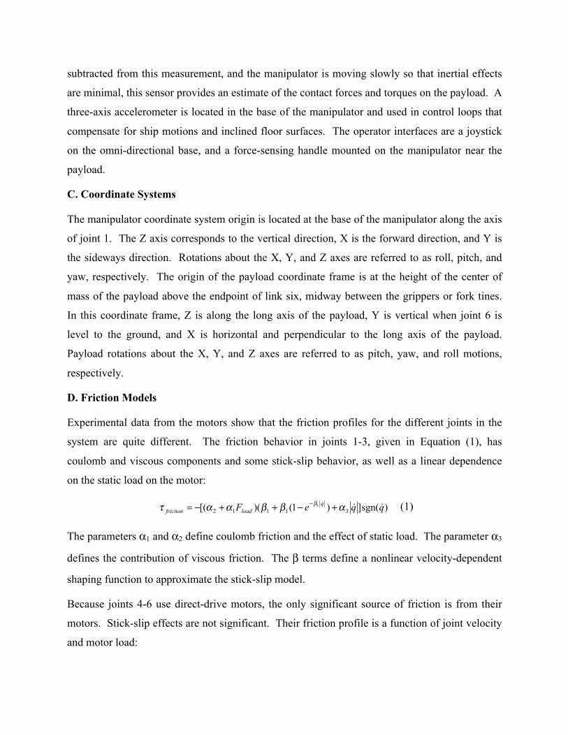
A. Position Control
The load cells in joints 1-3 allows the use of sensor based torque control to compensate for the
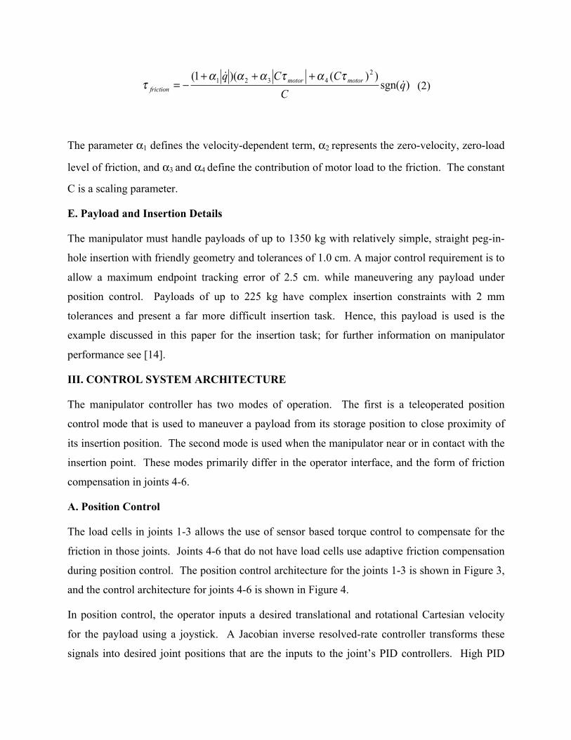
friction in those joints. Joints 4-6 that do not have load cells use adaptive friction compensation
during position control. The position control architecture for the joints 1-3 is shown in Figure 3,
and the control architecture for joints 4-6 is shown in Figure 4.
In position control, the operator inputs a desired translational and rotational Cartesian velocity
for the payload using a joystick. A Jacobian inverse resolved-rate controller transforms these
signals into desired joint positions that are the inputs to the joint’s PID controllers. High PID
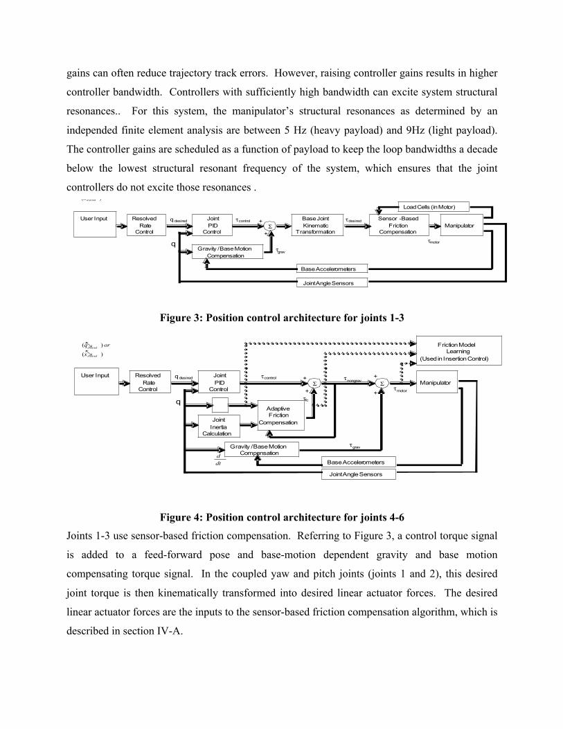
gains can often reduce trajectory track errors. However, raising controller gains results in higher
controller bandwidth. Controllers with sufficiently high bandwidth can excite system structural
resonances.. For this system, the manipulator’s structural resonances as determined by an
independed finite element analysis are between 5 Hz (heavy payload) and 9Hz (light payload).
The controller gains are scheduled as a function of payload to keep the loop bandwidths a decade
below the lowest structural resonant frequency of the system, which ensures that the joint
controllers do not excite those resonances .
JointPID
Control
qdesired Sensor -Based Friction
Compensation
Gravity / Base MotionCompensation
+
+Manipulator
Base JointKinematic
Transformation
Resolved Rate
Control
τdesired
τmotor
τcontrol
Σ
τgrav
q
Position Control System Joints 1 -3
User Input
)(
)(
d esired
d esired
x
orq
Joint Angle Sensors
Base Accelerometers
Load Cells (in Motor)
Figure 3: Position control architecture for joints 1-3
JointPID
Control
qdesired
Gravity / Base MotionCompensation
+
+Resolved Rate
Control τmotor
τcontrol
Σ
τgrav
q
Σ
Adaptive Friction
Compensation
dtd
+
JointInertia
Calculation
+
τnongrav
τfc
User Input
)(
)(
d esired
d esired
x
orq Friction Model
Learning(Used in Insertion Control)
Joint Angle Sensors
Manipulator
Base Accelerometers
Figure 4: Position control architecture for joints 4-6
Joints 1-3 use sensor-based friction compensation. Referring to Figure 3, a control torque signal
is added to a feed-forward pose and base-motion dependent gravity and base motion
compensating torque signal. In the coupled yaw and pitch joints (joints 1 and 2), this desired
joint torque is then kinematically transformed into desired linear actuator forces. The desired
linear actuator forces are the inputs to the sensor-based friction compensation algorithm, which is
described in section IV-A.

In joints 4-6, the control torque signal is added to a friction compensation torque signal
from an adaptive algorithm. This friction compensation algorithm uses an observer to
compensate for all uncompensated disturbances to the joint, and is discussed in section IV-B. It
requires the joint velocity, joint inertia, and the sum of all non-disturbance torques applied to the
joint as inputs. The gravity and base motion compensation torque is calculated the same way as
for the joints 1-3. Gravity and gravity compensation are assumed to offset, and any difference in
the two is treated as a disturbance. The friction parameters are learned during this time for use
during insertion control.
B. Admittance Based Insertion Control
The insertion controller allows an operator insert the payload in its rack even when the view of
the insertion lugs on the payload and the mating slots on the loading rack are obstructed by the
payload. See Figure 5 for conceptual diagram of the insertion controller. The operator applies
force and torque to the insertion control handle, which is mounted on a force/torque sensor. This
force/torque combination (wrench) is then vectorially added to an estimate of the contact wrench
acting on the payload. The contact wrench is approximated by subtracting the weight of the
payload from a measurement of the force between the payload and the manipulator. If the model
of the payload is correct, and the inertial forces from motion of the payload are small, this
approximation is accurate. The combined wrench from the user and the payload force sensors is
the input to an admittance control law, which calculates a desired endpoint velocity of the
manipulator. A purely viscous admittance law, which translates a desired force into a
proportional desired endpoint velocity, was chosen for this application [41,9]. The desired
endpoint velocity is then integrated and used as the input to a position controller.
During insertion control mode, the operator grasps the control handle, and can watch the motion
of the payload and feel the response of the manipulator to his input forces. When an operator
brings the payload into contact with the environment, the control law uses the feedback from the
payload force to command the manipulator to come to rest against the environment, and exert a
force on the environment equal to the user force on the input handle. Effectively, the payload
moves easily in directions where it does not contact the environment, and the manipulator does
not attempt to push the payload through the environment any harder than the user is pushing on
the force handle. The forces caused by the payload interaction with small environmental features

cause the controller to alter the motion of he payload in such a manner that the operator can
determine the location of the interference, and adjust his inputs accordingly. For example, if an
operator is pushing a payload in a straight line, and the payload began to rotate about some point,
the operator could both see and feel that the interference is occurring at that point. The
operator’s tactile feedback, combined with the knowledge of what forces he applied and the
payload interaction geometry, allows the operator to formulate a mental model to compensate for
the obstructed view of the insertion and the lack of bilateral force feedback..
Figure 5: Description of the insertion control concept.
During insertion control mode, the sensor-based friction compensation algorithm in joints 1-3 is
identical to the compensation algorithm in position control mode, as it is stable in the presence of
contact forces. However, it is difficult to make the adaptive friction compensation used in joints
4-6 stable in the presence of contact forces. Therefore, during insertion control, joints 4-6 use
model-based feed forward friction compensation. The parameters of this model are learned
during position control motions from the output of the adaptive friction compensation. Details of
the feed-forward compensation and learning process are discussed in section IV-C.
IV: FRICTION COMPENSATION
A. Joints 1-3: Torque Control Loops
The force sensors in the first three joints of the manipulator are located between the end of the
roller screw of the linear actuators that power the joints, and the linkage of the joint itself. This
allows a reliable measurement of the force transmitted through this point in the manipulator. The
force at the end of the linear actuator is related to the motor torque by:
LR
F gmeasureLoadcell
πτ
2= (3)
where L is the lead of the roller screw, and Rg is the transmission gear ratio. The error between
this measured torque and the desired torque is input into a PI controller that ensures the actual
torque applied to the joint tracks its desired value [11]. The gains in the torque control loops are
selected so that their bandwidth is approximately ten times the bandwidth of the PID controllers.
B. Joints 4-6 Position Control: Adaptive Friction Compensation
The adaptive estimator used here has been shown to provide accurate online estimates of friction
in position control systems, without regard to the model of the friction [12, 13]. A proof of the
Lyapunov stability of this adaptive algorithm is given in [13]. The algorithm is based on a
simple dynamic model of the joint:
αττ Ifricapp =+ (4)
where I is the effective joint inertia, α is the joint angular acceleration, τapp is the applied torque
by the controller, and τfric is the disturbance torque that is assumed to be friction. The effective
joint inertia is a function of the manipulator configuration, and is defined as the moment of
inertia of the links of a manipulator beyond a joint, about that joint. The applied torque (τapp) is
the sum of the uncompensated torques commanded to the joint by the controller. In this
manipulator, the applied torque is the sum of contributions of the PID controllers (τPID) and the
friction compensation torque (τfc) (see Equation (5)).
fcPIDapp τττ += (5)
Disturbance torques can come from many sources, such as friction, wind, contact forces, gravity
compensation errors, or an operator pushing on the manipulator. Because the friction
compensation works at the joint level, torque resulting from movement of the other joints is a
disturbance, as well.
The algorithm identifies the magnitude of the disturbance force (â) through the use of an
observer. It is assumed by the algorithm that all disturbances are the result of friction in the
joint, and the algorithm attempts to identify and cancel out this disturbance. The algorithm will
converge to the actual value of the disturbance so long as there is sufficient excitation for the

observer. For practical purposes, this means that the algorithm will correctly identify friction
whenever the joint is moving, as long as other disturbances are sufficiently low. A friction
compensation torque is then applied as the estimated magnitude â times the sign of the velocity
through the control law. The intermediate variable z is found using the adaptation law (see
Equations 6, 7, and 8).
)sgn(ˆ qafc =τ (6)
µqIkza −=ˆ (7)
)sgn(][1 qqkz fcapp ττµ µ −= − (8)
where q is the joint angle and k and µ are gains tuned for individual joints. In the case of this
manipulator, the applied torque less the friction compensation torque is the torque from the PID
controllers. In other cases, however, applying a shaping function such as a saturation function,
low pass filter, or a gain to the friction compensation torque may be useful to reduce effects such
as chatter.
The adaptive estimates from this algorithm, as well as the joint velocity and command torque are
recorded for use in the model-based feed-forward algorithm used during insertion control mode.
Dynamic disturbances from motions of other joints can lead to inaccurate identification of the
magnitude of friction at a given time, and therefore inaccurate identification of the parameters of
the friction model. For this reason, the friction parameter identification works best when only
one joint is moving at a time, or when the dynamic interactions between joints is small. The
motions of this manipulator generally fall within these boundaries.
C. Joints 4-6 Insertion Control: Model-Based Compensation
Since adaptive compensation is not feasible when the manipulator is in contact with the
environment, model-based feed forward friction compensation is used during insertion in joints
4-6. The form of the friction was developed based on experimental data (see Equation (2)). As
mentioned in the previous section, the data recorded by the adaptive friction compensators
during free motion of the manipulator is used to identify the parameters of this friction model.
Updating the parameters of the friction model enables the feed-forward friction model to track
changes in friction due to environmental conditions or wear over time. To the author’s
knowledge, this is a novel method of compensating for friction in contact with the environment.
Accurate parameter identification requires that data be cropped to eliminate points where the
estimate of friction is not likely to be accurate, such as when joint velocity is near zero, and
during any learning transients. The cropped data is used in a recursive nonlinear least-squares
curve-fit to identify the friction model parameters α1, α 2, α 3, and α 4. The parameters are then
averaged with other recent estimates.
The feed-forward friction compensation must not introduce any instability into the overall
controller. In order to ensure that the controller is robust to errors in the friction model, an
uncertainty torque is subtracted from the feed-forward friction torque, ensuring that the joint
controllers are not overcompensating for the joint friction [35]. The uncertainty in the friction
model will be evaluated on a joint by joint basis, based on the simulated and experimental
performance of the friction parameter identification algorithm.
V. SIMULATION RESULTS
A dynamic simulation of the full system was used to verify the friction compensation algorithms.
A representative model, seen in Figure 6, was constructed in MSC ADAMS, and interfaced with
a Simulink controller running at a time step of 0.001 s. The PID gains used in the joint
controllers were tuned 0.9 Hz, one decade below 9 Hz, the lowest structural natural frequency of
the system obtained from an independent finite element analysis. The joint friction was
implemented in the Simulink controller utilizing the models described in section II-C. During
the insertion control tests, the model also contains simulated insertion geometry that provides
contact force between the payload and the environment, in this case a loading rack. The loading
rack is modeled with a slot running the length of the rack, and the payload has two T-shaped lugs
that fit into the slots. The tolerances between the lugs on the payload and the slot are shown in
Figure 7.

Figure 6: The simulation system
Figure 7: Cross-section of the insertion geometry of the simulated system
A. Position Control Representative Task
A representative trajectory was selected to evaluate the performance of the position control
architecture. This trajectory includes payload acquisition, maneuvering into a carrying position,
and maneuvering the payload close to the insertion rack. The tracking error over this trajectory
of the manipulator with friction compensation is compared to a case without friction, and a case
with no friction compensation, see Figure 8. The tracking error is the endpoint deviation from
the desired trajectory, and the assumed permitted error is 2.5 cm.

Figure 8: Tracking error comparison for the representative task
The frictionless manipulator easily meets the permitted tracking error requirement during the
task. The manipulator with uncompensated friction has errors well above the 2.5 cm
specification, showing the need for joint friction compensation. Figure 8 shows that friction
compensation dramatically improves the performance. The errors of the robot with friction
compensation are only slightly higher than the frictionless robot, and far smaller than the errors
with uncompensated friction. The largest tracking errors are only about 1.6 cm, well within the
position control mode goal of 2.5 cm.
B. Friction Extraction
During the position control mode the friction magnitude in joints 4-6 is estimated by the adaptive
compensation algorithm. Figure 9 compares the estimate of friction from the adaptive
compensator with the actual value of friction used by the simulation. . It can be seen that the
adaptive algorithm estimates the friction very well. It is difficult to distinguish the two curves in
Figure 9.
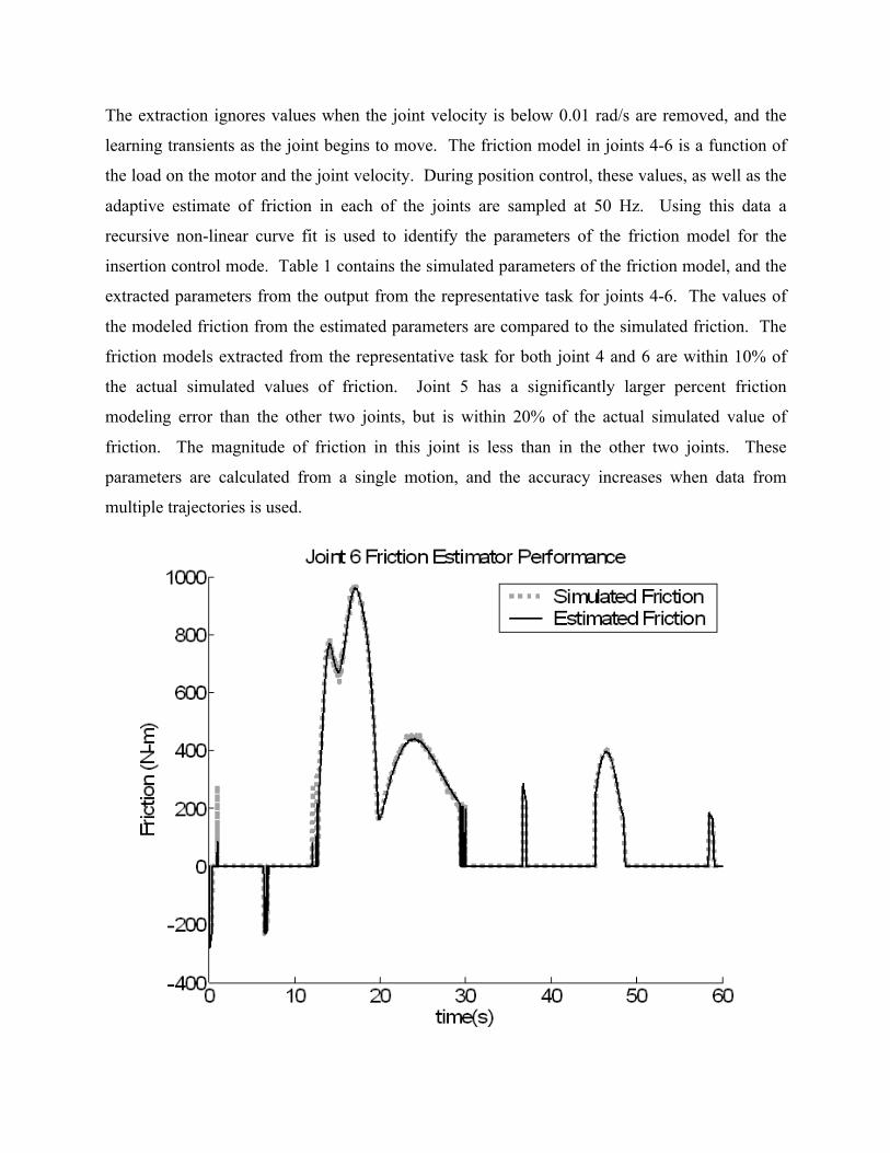
The extraction ignores values when the joint velocity is below 0.01 rad/s are removed, and the
learning transients as the joint begins to move. The friction model in joints 4-6 is a function of
the load on the motor and the joint velocity. During position control, these values, as well as the
adaptive estimate of friction in each of the joints are sampled at 50 Hz. Using this data a
recursive non-linear curve fit is used to identify the parameters of the friction model for the
insertion control mode. Table 1 contains the simulated parameters of the friction model, and the
extracted parameters from the output from the representative task for joints 4-6. The values of
the modeled friction from the estimated parameters are compared to the simulated friction. The
friction models extracted from the representative task for both joint 4 and 6 are within 10% of
the actual simulated values of friction. Joint 5 has a significantly larger percent friction
modeling error than the other two joints, but is within 20% of the actual simulated value of
friction. The magnitude of friction in this joint is less than in the other two joints. These
parameters are calculated from a single motion, and the accuracy increases when data from
multiple trajectories is used.

Figure 9: Friction estimator performance in joint 6 during the representative task Table 1: Actual and extracted curve-fit parameters of friction
Joint Simulated/ Extracted
α1 (s/rad)
α2 (Nm)
α3 (no dim)
α4 (N-1m-1)
4 Simulated 10 500 0.187 -1*10-6 4 Extracted 9.78 484.4 0.184 -7.2*10-7 5 Simulated 10 150 0.187 -1*10-6 5 Extracted 12.03 122.6 0.160 -2.6*10-6 6 Simulated 10 350 0.187 -1*10-6 6 Extracted 10.7 335 0.177 -1.3*10-6
C. Insertion Control Mode – Admittance Law Stability
The admittance law must be tuned so that the environmental interaction does not lead to
control instabilities or excitation on the resonant frequencies of the manipulator.
A stable admittance law will have a bandwidth sufficiently low to avoid manipulator
structural resonances, as well as to avoid resonances arising from the payload-environment
interaction. A vibration analysis as proposed in [11] and modified to add a gripper compliance
and separate payload as in [37] may be used to determine a range of stable admittance laws for
the insertion controller. In this analysis, the response of the robot to endpoint disturbances is
linearized in the vertical direction with the manipulator arm outstretched.
The model shown in Figure 10 is used to derive state space equations for the robot. The
system is approximated as a one-directional, sixth order system of vibrating masses. These
masses are the robot, sensor, and payload of the manipulator. A state space vector is constructed
of the positions and velocities of these masses.
MR M s MP
KR Ks KG KP/E
BR Bs BGBP/E
XR Xs XP
F
MR M s MP
KR Ks KG K
BR Bs BG
XR Xs XP
Fcontrol
Subscript R: RobotSubscript S: SensorSubscript G: GripperSubscript P: PayloadSubscript P/E: Payload -Environment Interaction
State -Space Inputs and OutputsInput: Controller ForceOutput 1: Robot PositionOutput 2: Contact Force
= Fcontrol
= X R
= K S(XS-XR )
Figure 10: 6th-order model used for tuning the admittance law (Adapted from DiCicco [2])
The state space equations (9) describe the system and its response to the controller force F. The
output equations (10) describe outputs of the system, which are XR, the endpoint position of the

robot, and FC, the force sensed by the contact force sensor. The transfer functions from F to XR
and FC will be referred to as TFXR(s) and TFFC(s), respectively.
FM
X
MBB
MB
MKK
MK
MB
MBB
MB
MK
MKK
MK
MB
MBB
MK
MKK
VVVXXX
XR
P
EPC
P
C
P
EPC
P
C
S
C
S
CS
S
S
S
C
S
CS
S
S
R
S
R
SR
R
S
R
SR
P
S
R
P
S
R
⋅
⎥⎥⎥⎥⎥⎥⎥⎥
⎦
⎤
⎢⎢⎢⎢⎢⎢⎢⎢
⎣
⎡
+⋅
⎥⎥⎥⎥⎥⎥⎥⎥⎥⎥⎥
⎦
⎤
⎢⎢⎢⎢⎢⎢⎢⎢⎢⎢⎢
⎣
⎡
+−+−
+−+−
+−+−=
⎥⎥⎥⎥⎥⎥⎥⎥
⎦
⎤
⎢⎢⎢⎢⎢⎢⎢⎢
⎣
⎡
=
00
1000
)(0)(0
)()(
0)(0)(100000010000001000
//
(9)
FXKKF
X
SSC
R ⋅⎥⎦
⎤⎢⎣
⎡+⋅⎥
⎦
⎤⎢⎣
⎡−
=⎥⎦
⎤⎢⎣
⎡00
0000000001
(10)
Where R signifies robot, S is sensor, G is gripper, and P/E is payload and environmental
interaction. The controller force F is approximated as a PID controller with natural damping,
with a transfer function of the form (11).
IPND
IPD
KsKsKIsKsKsK+++
++23
2
(11)
The inertia term I is determined by calculating the inertia of the robot arm about the endpoint of
the robot and the control gains are calculated by tuning a PID controller with natural damping
with the same damping factor and bandwidth as the joint controllers for the calculated inertia. A
full listing of the identified and calculated parameters this system, as well as further details of
this stability analysis are found in [4].
Once the parameters of the system have been identified, the transfer function between
applied user force and applied force of the manipulator on the environment may be calculated as
a function of the admittance law. The closed loop position controller transfer function is shown
in (12)
)()(1)()(
sCsTFsCsPC
XR ⋅+= (12)
where s
KsKsKsC IPD ++=
2
)( (13)
As mentioned in section III-B, the admittance law is chosen so that desired payload velocity is
directly proportional to the contact force.
sKsA A=)( (14)
A closed loop transfer function between input force and output force (A.9) can be calculated
using the admittance law, position controller, and controller force to contact force transfer
function in the forward path with unity feedback.
)()()(1)()()(
)(sTFsPCsAsTFsPCsA
sGCF
CF
+= (15)
The bandwidth of the function G(s) must be limited to a decade below the structural natural
frequency of the manipulator, or a decade below any resonant frequencies of the payload-
gripper-environment interaction system, whichever is less.
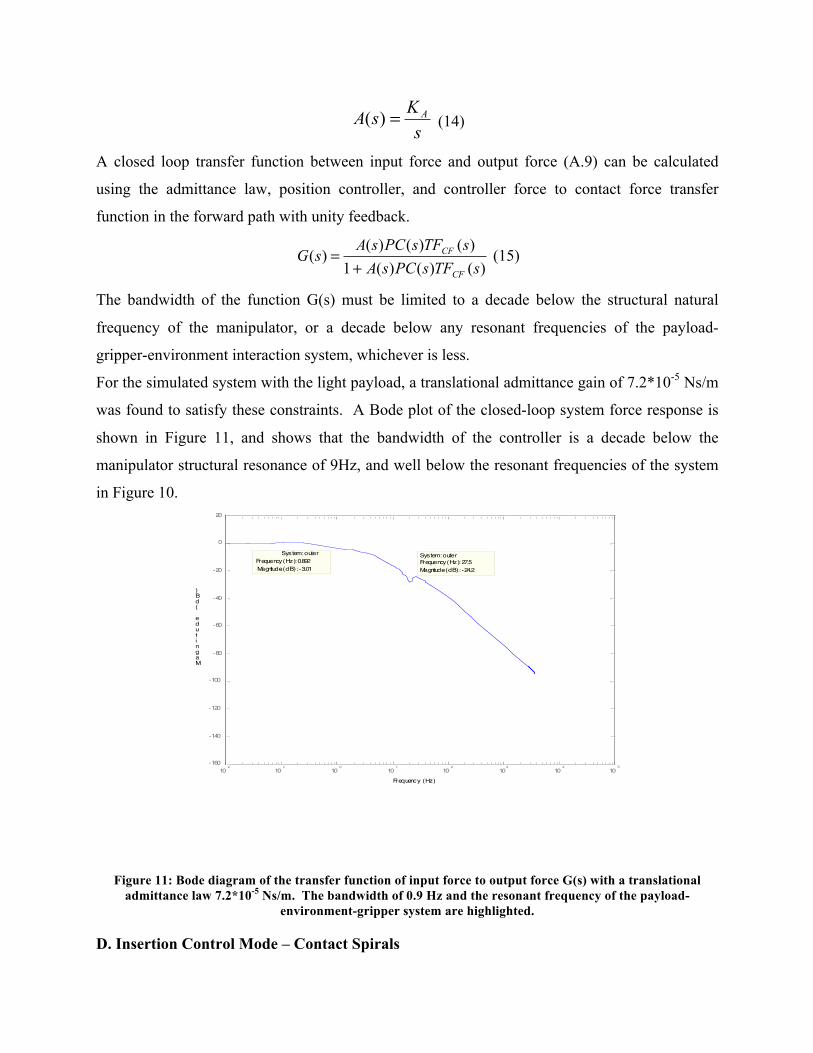
For the simulated system with the light payload, a translational admittance gain of 7.2*10-5 Ns/m
was found to satisfy these constraints. A Bode plot of the closed-loop system force response is
shown in Figure 11, and shows that the bandwidth of the controller is a decade below the
manipulator structural resonance of 9Hz, and well below the resonant frequencies of the system
in Figure 10.
10-2
10-1
100
101
102
103
104
105
-160
-140
-120
-100
-80
-60
-40
-20
0
20
System: outer Frequency (Hz): 0.892 Magnitude (dB): -3.01
System: outer Frequency (Hz): 27.5 Magnitude (dB): -24.2
Magnitude (dB)
Bode Diagram
Frequency (Hz)
Figure 11: Bode diagram of the transfer function of input force to output force G(s) with a translational admittance law 7.2*10-5 Ns/m. The bandwidth of 0.9 Hz and the resonant frequency of the payload-
environment-gripper system are highlighted.
D. Insertion Control Mode – Contact Spirals
A gain of 0.9 is used on the output of the friction model during insertion control to ensure that
the friction is never overcompensated. The performance of the feed-forward friction
compensation algorithm in a simulated task of the robot in contact with the environment is seen
in Figure 12. In this simulation, the payload is lifted into contact with a flat surface. The
commanded force is then reduced to 25N. For 15 seconds, an additional operator force is applied
in the plane of the surface. This force increases from 0 to 120 N at a constant rate, and the
direction of the force rotates within the plane every 4 seconds. This force input should result in
an expanding spiral motion of the manipulator endpoint while maintaining contact with the
surface. The actual and desired manipulator endpoint trajectories during this simulation are
shown in Figure 12 for a case with joint friction compensation.
During the simulation, the contact force normal to surface should remain constant at 125 N,
which is equal to the operator input force of 25N multiplied by the operator gain of 5 used for
this case. If the normal force has large variations, the corresponding friction variations cause the
manipulator to move intermittently along the surface, instead of smoothly, which is desirable for
the operator to make fine movements. Without friction compensation, the contact force varies
between -325N (2.6 times the expected value) and approximately -1N (where the manipulator
has almost lifted off of the rack), as seen in Figure 13. This variance from the desired force of
125N is due to tracking errors from uncompensated joint friction, as well as friction between the
payload and the environment. This large variance would make it very difficult for a user to
finely position the manipulator and complete an insertion task. Figure 14 shows the contact
force during the contact spiral simulation with friction compensation. The contact force varies
between -47 and -182. Examination of Figure 14 shows that the peak force tracking errors are
periodic. These peaks occur when joints of the manipulator change direction to follow the
desired path. While the force tracking errors are significant, they occur at predictable times, and
are never large enough to cause the payload to come close to leaving contact with the rack
Implementing the feed-forward friction compensation greatly improves the ability of the
manipulator to maintain a desired contact force.

Figure 12: Actual and desired trajectory during the contact spiral simulation

Figure 13: Contact force normal to the plane of the surface during the contact spiral simulation without joint friction compensation

Figure 14: Contact force normal to the plane of the surface during the contact spiral simulation with joint friction compensation
D. Insertion Control Representative Task
Because human operators are difficult to model, the simulation uses simple inputs to evaluate the
effectiveness of the insertion controller. Figure 15 shows a view looking down the insertion slot
of the rack during an insertion task. First, the manipulator is commanded to hold the payload
several centimeters below the slot. The payload is initially misaligned with the slot by three
degrees about the pitch (payload X) and yaw (payload Y) axes. After 2 seconds, a force
command, represented by the white arrow, of 100N is applied in the positive Y direction to the
manipulator. At 5 seconds, the rear lug contacts the insertion rail. This impact results in a
contact torque about the X axis of the manipulator endpoint, and the control system reacts by
rotating the payload in the direction of the torque. At 8 seconds, this rotation results in the
impact of the front lug with the insertion rail. At this time, a 100N force in the negative X
direction in addition to the 100N force in the positive Y direction is applied. The manipulator
then moves along the rail until 11 seconds, when the rear lug enters the insertion slot, resulting in
a torque about the Y axis of the payload. The manipulator then rotates the payload, and at 12
seconds the second lug enters the insertion slot, ending the insertion task.
The simulated insertion task demonstrates the effective compliance of the manipulator to the
effects of contact forces. When the manipulator is pushed into a misaligned rack, the controller
uses the contact forces to align the payload with the rack. As the payload is pushed across the
rack and a single lug partially enters the slot, the torque resulting from this partial engagement
aligns the other lug with the insertion slot. The successful insertion task with a misaligned
payload and simple open-loop force inputs suggests that a human operator should be able to use
the insertion controller to exploit environmental forces to aid in payload insertion tasks.

Figure 15: Simulated insertion task
VI. EXPERIMENTAL RESULTS
The full-scale manipulator had not yet been fully assembled and was not available for
experimental evaluation at the writing of this paper. Therefore, the control algorithms developed
here have been implemented on a reduced degree-of-freedom laboratory manipulator to provide
some experimental validation of the control algorithms. The robot is not equipped with joint-
level load cells for sensor-based friction compensation, so the control architecture for the
experimental system is the same as joints 4-6 in the full-scale manipulator. The joint position
controllers are tuned to a 1 Hz bandwidth, which is approximately the bandwidth of the joint
controllers on the full scale manipulator with the light payload. During position control, all
joints have adaptive friction compensation, and during insertion control all joints have model-
based feed-forward friction compensation. The absence of joints using sensor-based friction
compensation is acceptable because the torque loops in those joints are well-studied [28,33].
The laboratory robot enables an evaluation of the more novel aspects of the controller: utilizing
adaptive friction compensation to formulate a model of friction for use in contact with the
environment, and the insertion control mode.
The system is an AdeptOne robot. It is shown with its kinematic configuration in Figure 16. It
is a 4 degree of freedom manipulator, which allows the end effector and payload to be translated
in three axes, and rotated about the world yaw axis. The robot is equipped with two six axis
force/torque sensors that allow sensing of operator input and estimation of contact forces. The
operator input sensor is located under a handle which rotates with the end link. The payload
force sensor is located along the axis of joint 4, below the attachment point of the operator force
handle. The payload is mounted below the force sensor, and consists of a cylinder with two lugs.
The lugs and the mating geometry of the lugs have tolerances of approximately ½ that of the full-
scale manipulator. The robot is equipped with position encoders on each joint.

Payload
X
Z
Y
Payload Force Sensor
(Manipulator Endpoint)
UserHandle
User Force Sensor
Joint 1 Joint 2
Joint 4
Joint 3
Figure 16: The experimental system
A. Position Control Trajectory
The ability of the adaptive friction algorithm to reduce tracking errors during position control is
shown in Figure 17. For this case, the desired trajectory is a square in the horizontal
(manipulator X-Y) plane. Figure 17 shows the tracking error with and without friction
compensation. The manipulator with uncompensated friction had a maximum tracking error of
2.96 cm. and an average tracking error of 0.79 cm. The maximum tracking error was reduced to
1.50 cm., and the average tracking error was only 0.20 cm with adaptive friction compensation.
Clearly, the adaptive friction compensation algorithm can reduce position control tracking errors.
B. Friction Model Extraction
To identify the form and parameters of the joint friction models, the response of the manipulator
to a sinusoidal joint input was studied. Figure 18 shows the friction estimate from joint 2
following this trajectory as a function of joint velocity. It appears to be a parabolic function with
a peak value of 3.6 Nm at zero velocity. The magnitude of the friction estimate does not vary
widely, so a simple Coulomb model can be used to approximate the friction. The adaptive
estimator data is fit to this model, and the Coulomb friction parameter a1 is identified as:
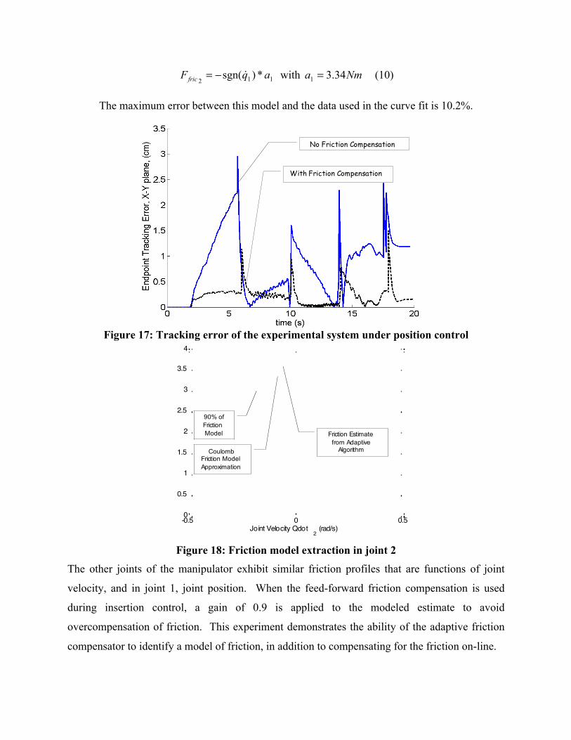
112*)sgn( aqFfric −= with Nma 34.31 = (10)
The maximum error between this model and the data used in the curve fit is 10.2%.
Experimental Position Control
No Friction Compensation
With Friction Compensation
Figure 17: Tracking error of the experimental system under position control
-0.5 0 0.50
0.5
1
1.5
2
2.5
3
3.5
4Friction Model from Adaptive Estimates, Joint 2
Joint Velocity Qdot2 (rad/s)
Friction Estimate (N/m)
90% of Friction Model
Coulomb Friction ModelApproximation
Friction Estimate from Adaptive
Algorithm
Figure 18: Friction model extraction in joint 2
The other joints of the manipulator exhibit similar friction profiles that are functions of joint
velocity, and in joint 1, joint position. When the feed-forward friction compensation is used
during insertion control, a gain of 0.9 is applied to the modeled estimate to avoid
overcompensation of friction. This experiment demonstrates the ability of the adaptive friction
compensator to identify a model of friction, in addition to compensating for the friction on-line.

C. Insertion Task
During insertion control, the user grasps the force handle of the robot, and maneuvers a payload
into contact with the environment. An analysis similar to that shown in section V-C was used to
determine stable admittance laws for the contact force feedback and operator input [4]. An
insertion payload and mating geometry were constructed for the experimental system to
approximate a ½ scale light payload. This payload is shown in Figure 19. Tests were performed
where operators were asked to insert the payload into the insertion slots and slide the payload
forward, simulating locking the payload into place, as seen in Figure 20. Operators were asked
to perform the task using only visual feedback, controlling the manipulator from a controller
fixed to ground. Operators also attempted to insert the payload using both visual and tactile
feedback, using the force sensor mounted on the manipulator endpoint to control the robot, as
seen in Figure 21.
Figure 19: The two lug payload and insertion geometry
Operators were able to perform successful insertions in both the visual feedback only and visual
and tactile feedback cases. However, the addition of tactile feedback greatly increased the speed
with which an operator could perform the insertion task, and the speed which an operator could
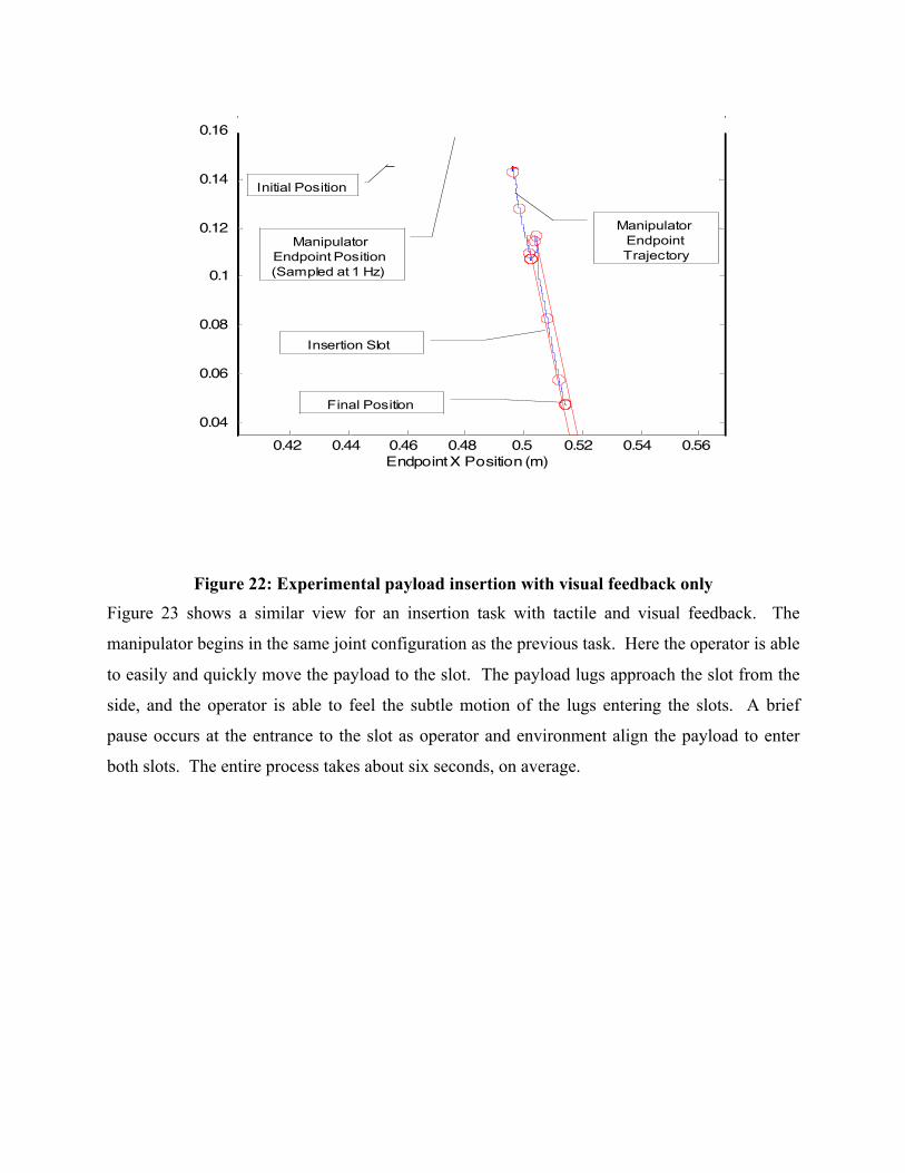
correct for a mistake made during the insertion process. Figure 22 shows the overhead view of
the trajectory of the manipulator endpoint during a typical insertion using only visual feedback.
The solid line represents the trajectory, the circles are the position of the manipulator sampled at
1 Hz, and the dotted line represents the border of the insertion slot. The operator, moving
slowly, is careful and moves the payload sideways and makes fine rotational adjustments so it is

aligned with the slots. The operator then moves the payload forward until both lugs approach
their slots. After several small adjustment motions, the lugs of the payload enter the slot, and the
operator can push the payload forward into place. The entire process takes approximately 17
seconds on average.
6
Rear Lug inRear Slot
(moved forward)
Front Lug inFront Slot
(moved forward)
Figure 20: The payload after a successful insertion task has moved forward in the slot
Figure 21: The manipulator under insertion control with visual and tactile feedback
0.42 0.44 0.46 0.48 0.5 0.52 0.54 0.560.04
0.06
0.08
0.1
0.12
0.14
0.16
Insertion Task, Visual Feedback Only
Endpoint X Position (m)
Endpoint Y Position (m)
Manipulator Endpoint Trajectory
Manipulator Endpoint Position (Sampled at 1 Hz)
Insertion Slot
Final Position
Initial Position
Figure 22: Experimental payload insertion with visual feedback only
Figure 23 shows a similar view for an insertion task with tactile and visual feedback. The
manipulator begins in the same joint configuration as the previous task. Here the operator is able
to easily and quickly move the payload to the slot. The payload lugs approach the slot from the
side, and the operator is able to feel the subtle motion of the lugs entering the slots. A brief
pause occurs at the entrance to the slot as operator and environment align the payload to enter
both slots. The entire process takes about six seconds, on average.

0.42 0.44 0.46 0.48 0.5 0.52 0.54 0.56
0.04
0.05
0.06
0.07
0.08
0.09
0.1
0.11
0.12
0.13
0.14
Insertion Task, Visual and Tactile Feedback
Endpoint X Position (m)
Endpoint Y Position (m)
Manipulator Endpoint Trajectory
Manipulator Endpoint Position (Sampled at 1 Hz)
Insertion Slot
Final Position
Initial Position
Figure 23: Experimental Payload insertion with visual and tactile feedback
The experimental tests of the insertion controller confirm that the presence of position tactile
feedback from a manipulator significantly improves the ability of an operator to insert the
payload. The improved performance as a result of tactile feedback is further demonstrated by the
ability of many operators to insert the payload when wearing a blindfold after some practice
using the manipulator. The operator is able to construct a mental model of the payload and
environment interaction, and from the tactile feedback of the manipulator is able to determine
where the payload is in relation to the insertion slot, and successfully insert the payload.
However, this situation requires a substantial increase in the time required to complete the task.
VII. CONCLUSION
In this paper, a control architecture is developed for a heavy-lift manipulator required to perform
precision insertion tasks in a harsh environment. A major component of this control architecture
is a friction compensation system that is able to significantly reduce the effects of joint friction
that varies over time. Another major component of the control architecture is an “insertion
control system” which allows the feedback of tactile clues of the position of the manipulator to
the operator to compensate for the lack of bilateral force feedback.

Simulation and experimental results show that the friction compensation architecture
significantly decreased the tracking error during position control. Simulation results demonstrate
the ability of an adaptive friction compensation algorithm to extract parameters of a known
model of friction. Experimental results show that the output from the adaptive algorithm could
be used to identify an unknown model of friction as well. Successful insertion tasks in
simulation using open-loop force commands, and experimentally with operators suggest that the
control architecture, when implemented on the full scale manipulator, will enable an operator to
load large payloads in a difficult environment.
VIII. ACKNOWLEDGEMENTS
The authors would like to acknowledge the support of Foster-Miller, Inc. and the United States
Navy for their support of this research, as well as Takeshi Takaura, and Matt Lichter for their
helpful comments and contributions during this work.
IX REFERENCES
1. Anderson, R.J., and M.W. Spong. "Bilateral Control of Teleoperators with Time Delay." IEEE Transactions on Automatic Control. Vol. 34, no. 5. pp. 494-501.
2. Armstrong B, Dupont P, Canudas-de-Wit C. “A Survey of Models, Analysis Tools and Compensation Methods for the Control of Machines with Friction.” Automatica, Vol. 30, Issue 7, pp. 1083-1138, July 1994.
3. Asada, H, and J.E. Slotine. Robot Analysis and Control. Wiley-IEEE, New York. 1986. 4. Becker, W. “The Design of a Control Architecture for a Heavy-Lift Precision
Manipulator for Use in Contact with the Environment.” Master’s Thesis. Mechanical Engineering Dept. Massachusetts Institute of Technology. 2006.
5. Canudas de Wit C., Lischinsky P. “Adaptive Friction Compensation with Partially Known Dynamic Friction Model.” International Journal of Adaptive Control and Signal Processing, Vol. 11, 65-80, 1997.
6. Chiaverini, S., B. Siciliano, and L. Villani. "A Survey of Robot Interaction Control Schemes with Experimental Comparison." IEEE/ASME Transactions on Mechatronics, Vol. 4, no. 3. pp 273-285. September 1999.
7. Craig, J.J., P.Hsu, and S.S. Sastry. "Adaptive Control of Mechanical Manipulators." Proceedings of the 1986 IEEE International Conference on Robotics and Automation, Vol. 3, pp. 190-195. April 1986.
8. Deeter T, Koury G, Rabideau K, Leahy M, Turner T. “The Next Generation Munitions Handler Advanced Technology Demonstrator Program.” Proceedings of the 1997 IEEE International Conference on Robotics and Automation, pp. 341-345, 1997.
9. DiCicco, M. “Force Control of Heavy Lift Manipulators for High Precision Insertion Tasks.” Master’s Thesis. Mechanical Engineering Dept. Massachusetts Institute of Technology. 2005.
10. Draper, J.V., F.G. Pin, J.C. Rowe, J.F. Jansen. "Next Generation Munitions Handler: Human-Machine Interface and Preliminary Performance Evaluation." ORNL/CP-101966, April 1999.
11. Eppinger, Steven D. and Warren P. Seering. “Introduction to Dynamic Models for Robot Force Control.” IEEE Control Systems Magaine. 1987. 48-52.
12. Friedland B, Mentzelopoulou S. “On Estimation of Dynamic Friction.” Proceeding of the 32nd Conference on Decision and Control, Vol. 2, 15-17, pp. 1919-1924, December 1993.
13. Friedland B, Park Y. “On Adaptive Friction Compensation.” IEEE Transactions on Automatic Control, Vol. 37, Issue 10, pp. 1609-1612, October 1992.
14. Garretson, J. “High-Precision Control of a Heavy-Lift Manipulator in a Dynamic Environment.” Master’s Thesis. Mechanical Engineering Dept. Massachusetts Institute of Technology. 2005.
15. Gomes S, Santos da Rosa V. “A New Approach to Compensate Friction in Robotic Actuators.” Proceedings. ICRA ’03. IEEE International Conference on Robotics and Automation, Vol. 1, 14-19, September 2003.
16. Hastrudi-Zaad, K. and S.E. Salcudean. “On the Use of Local Force Feedback for Transparent Teleoperation.” Proceedings, 1999 IEEE International Conference on Robotics and Automation. IEEE. 1999. Vol. 3. pp. 1863-1869.
17. Henrichfreise H, Witte C. “Experimental Results with Observer-Based Nonlinear Compensation of Friction in a Positioning System.” IEEE Intl. Conference on Robotics and Automation, Vol. 1, 16-20, May 1998.
18. Hogan, N. “Impedance Control: An Approach to Manipulation: Parts 1-3: Theory, Implementation, and Applications.” Journal of Dynamic Systems, Measurement and Control. 1985, Vol 107. 1-24.
19. Iagnemma K. “Manipulator Identification and Control Using a Base-Mounted Force/Torque Sensor.” Master’s Thesis, Department of Mechanical Engineering, MIT, 1997.
20. Jacobsen, S. C., I. D. McCammon, K. B. Biggers, and R. P. Phillips. “Tactile Sensing System Design Issues in Machine Manipulation.” IEEE. 1987. pp 2087-2096.
21. Kazerooni, H. “Extender: A Case Study for Human-Robot Interaction via Transfer of Power and Information Signals.” IEEE International Workshop on Robot and Human Communication, 1993. pp 10-20.
22. Kazerooni, H. and Ming-Guo Her. “The Dynamics and Control of a Haptic Interface Device.” IEEE Transactions on Robotics and Automation, Vol 10. No 4. 1994. pp 453-464.
23. Kazerooni, H., Tsing-luan Tsay, and Karin Hollerbach. “A Controller Design Framework for Telerobotic Systems.” IEEE Transactions on Control Systems Technology, Vol 1, No 1. 1993. pp 50-62.
24. Kim H, Cho Y, Lee K. “Robust Nonlinear Task Space Control for a 6 DOF Parallel Manipulator.” Proceedings of the 41st IEEE Conference on Decision and Control, Vol. 2, 10-13, December 2002.
25. Lischinsky P, Canudas-de-Wit C, Morel G. “Friction Compensation of a Schilling Hydraulic Robot,” Proceedings of the 1997 IEEE International Conference on Control Applications, 5-7, pp. 294-299, October 1997.
26. Love L, Jansen J, Pin F. “On the Modeling of Robots Operating on Ships.” Proceedings of the 2004 IEEE International Conference on Robotics and Automation, Vol. 3, pp. 2436-2443, April 26 – May 1, 2004.
27. Love, L.J., J.F. Jansen, and F.G. Pin. “Compensation of Wave-Induced Motion and force Phenomena for Ship-Based High Performance Robotic and Human Amplifying Systems.” ORNL/TM-2003/233. October, 2003.
28. Luh J, Fisher W, Paul R. “Joint Torque Control by Direct Feedback for Industrial Robots.” IEEE Transactions on Automatic Control, Vol. 28, No. 1, Feb. 1983.
29. Morel G, Iagnemma K, Dubowsky S. “The Precise Control of Manipulators with High Joint-Friction Using Base Force/Torque Sensing.” Automatica: Journal of the Int. Federation of Automatic Control, Vol. 36, No. 7, pp. 931-941, 2000.
30. Moreno J, Kelly R, Campa R. “Manipulator Velocity Control using Friction Compensation.” IEE Proceedings on Control Theory Applications, Vol. 150, No. 2, March 2003.
31. Niemeyer G, Slotine J. “Performance in Adaptive Manipulator Control.” Proceedings of the 27th IEEE Conference on Decision and Control, Vol. 2, 7-9, pp. 1585-1591, December 1988.
32. Olsson H, Astrom K, Canudas-de-Wit C, Gafvert M, Lichinsky P. “Friction Models and Friction Compensation.” European Journal of Control, Vol. 4, No. 3, 1998.
33. Pfeffer L, Khatib O, Hake J. “Joint Torque Sensory Feedback of a PUMA Manipulator.” IEEE Transactions on Robotics and Automation, Vol. 5, No. 4, pp. 418-425, 1989.
34. Seraji, H. “An On-Line Approach to Coordinated Mobility and Manipulation.” Proceedings of the 1993 IEEE International IEEE International Conference on Robotics and Automation, Vol. 1, pp. 28-35. May 1993.
35. Slotine, J.E. "Robust Control of Robot Manipulators." International Journal of Robotics Research. Vol. 4, no. 2, pp. 49-64. 1985.
36. Slotine, J.E. and W. Li "On the Adaptive Control of Robot Manipulators." International Journal of Robotics Research. Vol. 6, no. 3, pp. 49-59. 1987.
37. Volpe, Richard and Pradeep Khosla. “Analysis and Experimental Verification of a Fourth Order Plant Model for Manipulator Force.” IEEE Robotics and Automation Magazine. 1994. 4-13.
38. Whitcomb, L, S. Arimoto, T. Naniwa, and F. Ozaki. " Adaptive Model-Based Hybrid Control of Geometrically Constrained Robot Arms." IEEE Transactions on Robotics and Automation, Vol. 13, no. 1. February 1997.
39. Whitney, D.E., “Resolved Motion Rate Control of Manipulators and Human Prostheses.” IEEE Transactions on Man-Machine Systems, Vol. MMS-10 No. 2 June 1969.
40. Yamamoto, Y. and Yun, X. “Effect of the Dynamic Interaction on Coordinated Control of Mobile Manipulators” Proceedings IEEE Transactions on Robotics and Automation, Vol. 12, No. 5, pp. 816-824. Oct 1996.

41. Yu, H. “Mobility Design and Control of Personal Mobility Aids for the Elderly.” Ph. D. Thesis. Mechanical Engineering Dept. Massachusetts Institute of Technology. 2002.
APPENDIX: D-H PARAMETERS OF ROBOT
Link Axis Name αi ai (m) θi di (m) type Range
1 Base yaw π/2 0.1651 0 0 0 variable
2 Base pitch -π/2 0.2951 0 0 0 -95o to -25o
3 Arm extension π/2 0.0444 0 0 1 0.921 to 1.327 m
4 End pitch -π/2 0.3239 0 0 0 10o to 105o
5 End Yaw π/2 0 0 0.3810 0 -120o to 120 o
6 Roll (up to 1500 lb payload) 0 0.5080 0 0 0 -45o to 225o
6 Roll (1500 to 3000 lb load) 0 0.3810 0 0 0 -45o to 225o