Master's Degree Thesis ISRN: BTH-AMT-EX--2015/D11--SE

Supervisors: Maciej Wysocki and Mohammad Rouhi, SICOMP AB Sharon Kao-Walter, BTH

.

Department of Mechanical Engineering Blekinge Institute of Technology

Karlskrona, Sweden

2015

Waleed Ahmad Mirza

A Continuum Based Solid Shell Element Based on EAS and ANS

A Continuum Based SolidShell Element Based on EAS

and ANSWaleed Ahmad MirzaDepartment of Mechanical Engineering

Blekinge Institute of TechnologyKarlskrona, Sweden.

2015

Thesis submitted for completion of Master of Science in MechanicalEngineering with emphasis on Structural Mechanics at the Department ofMechanical Engineering, Blekinge Institute of Technology, Karlskrona,Sweden.

Abstract

This work is a stepping stone towards developing higher order shell element forsimulating composite manufacturing procedure. In this study, a continuumapproach suitable for combined material and geometrically nonlinear analysisfor an eight node solid shell element SS8 is explained. The formulation of SS8comprises two ingredients to alleviate undesirable locking effects: 1) AssumedNatural Strain concept, which has proven to alleviate the curvature thicknessand transverse shear locking problems. 2) Enhanced Assumed Strain, whichadds enhanced degrees of freedom to improve the in-plane response of theelement and the curvature thickness locking problem. This formulation hasbeen extended to represent geometric and material non-linearity using TotalLagrangian approach. Finally, finite strain formulation has been verified bynumerical examples. Results when compared to continuum shell element inABAQUS show a reasonable agreement with a relative error of less than 2%.

Keywords

Lagrangian, Finite Strain, Solid Shell Element, Enhanced Assumed Strain

Acknowledgement

This research work is carried out in Swerea SICOMP AB and Blekinge Insti-tute of Technology, Karlskrona, Sweden, under the supervision of Dr. MaciejWysocki, Dr. Mohammad Rouhi and Prof. Sharon Kao-Walter.

I am grateful to Dr. Maciej Wysocki who provided me the opportunity to con-duct this research. Moreover my sincere appreciation goes to Dr. MohammadRouhi for helping me with technical difficulties and to all my colleagues atSICOMP for providing me a conducive atmosphere to carry out this researchand above all for their valuable support and advice. Last but not least, myfather, mother and girlfriend, who owes my deepest gratitude and love forbeing an endless source of motivation for me.

Gothenburg, May 2015

Waleed Ahmad Mirza

Contents

1 Notation1.1 Variables . . . . . . . . . . . . . . . . . . . . . . . . . . . . . . . .1.2 Abbreviations . . . . . . . . . . . . . . . . . . . . . . . . . . . . . .1.3 Superscripts . . . . . . . . . . . . . . . . . . . . . . . . . . . . . . .1.4 Operators . . . . . . . . . . . . . . . . . . . . . . . . . . . . . . . .

2 Introduction2.1 Motivation . . . . . . . . . . . . . . . . . . . . . . . . . . . . . . .2.2 Solid Shell Elements – State of the art review . . . . . . . . . . . .2.3 Outline of thesis and proposed methodology . . . . . . . . . . . . .

3 Theory of Finite Strain Analysis3.1 Total Lagrangian Formulation . . . . . . . . . . . . . . . . . . . . .

3.1.1 Integrating EAS and TL Formulation . . . . . . . . . . . .

4 SS8 Formulation- Small Strain kinematics4.1 Linear Element Formulation . . . . . . . . . . . . . . . . . . . . . .4.2 Thickness Strain . . . . . . . . . . . . . . . . . . . . . . . . . . . .4.3 Transverse Shear Strain . . . . . . . . . . . . . . . . . . . . . . . .4.4 In-plane Strain Response . . . . . . . . . . . . . . . . . . . . . . . .4.5 Transformation to Orthonormal Coordinate System . . . . . . . . .4.6 Enhanced Strain . . . . . . . . . . . . . . . . . . . . . . . . . . . .4.7 Element Stiffness Matrix . . . . . . . . . . . . . . . . . . . . . . . .

5 SS8 Formulation- Finite Strain kinematics5.1 Geometric and Kinematic Formulation . . . . . . . . . . . . . . . .

5.1.1 Strain and Enhanced Strain Parametrization . . . . . . . .5.1.2 Internal load vectors . . . . . . . . . . . . . . . . . . . . . .

5.2 Stiffness Computation . . . . . . . . . . . . . . . . . . . . . . . . .5.3 Constitutive Equations of Hyperelasticity . . . . . . . . . . . . . .

4

5.4 Algorithm . . . . . . . . . . . . . . . . . . . . . . . . . . . . . . . .

6 Numerical Analysis6.1 Benchmarking . . . . . . . . . . . . . . . . . . . . . . . . . . . . . .6.2 Cantilever beam bending . . . . . . . . . . . . . . . . . . . . . . . .

6.2.1 Results . . . . . . . . . . . . . . . . . . . . . . . . . . . . .6.2.2 Discussion . . . . . . . . . . . . . . . . . . . . . . . . . . . .

6.3 Analysis of thin eam ( tL =30, 300 and 3000) . . . . . . . . . . . .

6.3.1 Conclusion . . . . . . . . . . . . . . . . . . . . . . . . . . .6.4 Cook’s Membrane Problem . . . . . . . . . . . . . . . . . . . . . .

6.4.1 Results . . . . . . . . . . . . . . . . . . . . . . . . . . . . .6.4.2 Discussion . . . . . . . . . . . . . . . . . . . . . . . . . . . .

6.5 Patch Test . . . . . . . . . . . . . . . . . . . . . . . . . . . . . . . .6.5.1 Result . . . . . . . . . . . . . . . . . . . . . . . . . . . . . .6.5.2 Discussion . . . . . . . . . . . . . . . . . . . . . . . . . . . .

6.6 Distortion test . . . . . . . . . . . . . . . . . . . . . . . . . . . . .6.6.1 Results . . . . . . . . . . . . . . . . . . . . . . . . . . . . .6.6.2 Discussion . . . . . . . . . . . . . . . . . . . . . . . . . . . .

7 Conclusion and Recommendations7.1 Conclusion . . . . . . . . . . . . . . . . . . . . . . . . . . . . . . .7.2 Learning outcomes . . . . . . . . . . . . . . . . . . . . . . . . . . .7.3 Future Work . . . . . . . . . . . . . . . . . . . . . . . . . . . . . .

8 References

9 Appendix9.1 Appendix A: Flow Diagrams . . . . . . . . . . . . . . . . . . . . .9.2 Appendix B: MATLAB Code . . . . . . . . . . . . . . . . . . . . .

Notation

Variables

Benh

BNL

B

B

b

Cijrs

c

D

E

t+�to E

eij

F

F

Enhanced strain displacement tensor

Non-linear strain displacement tensor

Non-linear strain displacement matrix

Linear strain displacement tensor

Left green Cauchy tensor

Component of Fourth order material tensor

Right green Cauchy stress

Energy dissipation

Elasticity modulus

Green Lagrangian strain tensor at time t + �t

Linear strain tensor

Deformation gradient

Transformation matrix

5

fenh Internal force due to enhanced strain matrix and stress state

Internal stress state tensor

Shear modulus

ith column of Jacobian matrix

ith column of spatial basis vector

Fourth order Identity Tensor

Determinant of deformation gradient

Linear stiffness tensor

Non-linear stiffness tensor

Spatial velocity gradient

Tensor of order 3x24 containing shape functions

Spatial normal to a surface

Shape function at node I

f

G

Gi

gi

I4

J

KL

KNL

l

N

n

NI

NkX Derivative of Shape function at node k with respect to spatial

coordinate X

P Stress power

R External load

S Second Piola-Kirchhoff stress

Sv Second Piola-Kirchhoff stress in vector formulation

t True traction vector

U 3 × 8 tensor representing displacement of each node of SS8

6

u Nodal displacement

ui,j Displacement component i with respect to component j

Vo Undeformed volume

v Poisson ratio

X, Y, Z Global coordinates( material coordinates)

x, y, z Deformed coordinates

ξ, η, ζ Natural coordinates

α Enhanced degree of freedom

ηij Non-linear strain tensor

εij Components of Green Lagrangian strain tensor

Ψ Free energy

τ Cauchy stress

σxx Longitudinal stress along x-axis

σyy Longitudinal stress along y-axis

σxy In plan sheer stress

Assumed Natural Deviatoric Strain

Assumed Natural Strain

Abbreviations

ANDES

ANS

EAS Enhanced Assumed Strain

7

SS8 Eight Node Solid Shell Element

Total Lagrangian

Updated Lagrangian

TL

UL

Superscriptsc Orthonormal Coordinate system

h Discrete

n Natural coordinate system

Operatorsδ Variation operator

(a ⊗ b)ijkl = (a)ij(b)kl with c : (a ⊗ b) = (c : a)b and (a ⊗ b) : c = (b : c)a

8

But these advantages come at cost of many undesirable phenomenas, popu-larly referred as locking effects [1]. Locking occurs when a shell element ismodelled like a solid brick element using displacement interpolation whichtends to ‘lock out’ realistic displacement of element response by activatingextraneous strains that require much higher energy input than strains of therealistic mode. These locking behaviours prevent solid elements to be usedfor shell like structures.

The goal of this project is to formulate an eight node solid shell element

9

Introduction

They are computationally effective and reliable in terms of capturing inplane and transverse response compared to brick elements. For instance, inapplication such as sheet metal deforming membrane stretching, bending andshearing are very dominant. In such scenario, solid shell elements can besuccessfully implemented to capture such intricate responses.

Unlike planer shell elements, using solid shell elements boundaries of threedimensional structures can be modelled without introducing any kinematicassumptions.

Shell elements are very efficient and robust in capturing mechanics ofstructures with thickness span much smaller than other two directions. Theseshell elements consist of arrange of subclasses, one of which is solid shellelements. Solid shell elements are in general modifies brick elements, capable tomodel thin shell or plate like structures. From literature review, solid shellelements are found to have following advantages over other families of shellelements [4].

reviewSolid shell elements are quite similar to brick elements in nodal formulationand exhibit only translational degree of freedom. Along with several advan-tages, these elements come with a number of disadvantages resulting fromsmaller span of thickness dimension compared to the lateral dimensions [1].Solid shell concept was developed to overcome well known degenerate concept.Using nodes at upper and lower surface and displacement degree of freedom,stresses and strains in longitudinal, transverse and thickness direction are cal-

10

based on continuum approach using isotropic hyper-elastic constitutive ma-terial model. This formulation is coupled with techniques such as AssumedNatural Strain (ANS) and Enhanced Assumed Strain (EAS) aimed at re-moving locking effects. First a solid shell element is formulated for smallstrain, linear kinematics and later extended to finite strain, nonlinear mate-rial kinematics using Lagrangian approach. At the end case studies have beenproposed to verify the formulation.

2.1 Motivation

This work is part of a bigger project aimed at developing a simulation tool formodelling composite manufacturing process of a wide range of popular infusiontechniques using higher order solid shell elements. Higher order shell elementshave extensive application in fields like porous media theory where pressurefield, a derivative of displacement, is approximated with linear variation [ ].As a consequence of linear pressure variation, the displacement is renderedquadratic. This quadratic displacement trend can be very well captured with a20 node solid shell element. Moreover, in other applications of structuralmechanics, higher order shell elements are better capable of capturing curvedgeometries.

The current project is a stepping stone towards developing higher order solidshell elements. The project involves formulating a 3D-shell element compris-ing 8 nodes based on hyper-elastic material model. The approach developedfor formulating eight node solid shell element will be used for modelling higherorder solid shell element in the follow up project. Such higher order elementwill be implemented in simulating composite manufacturing procedures likevacuum infusion.

2.2 Solid Shell Elements – State of the art

culated accurately. Along with several advantages, these elements come witha number of disadvantages resulting from smaller span of thickness dimensioncompared to the lateral dimensions. In literature several techniques such asANDES, ANS and EAS [1], [4] have been applied to overcome deficienciessuch as extra undesirable energy modes and locking phenomenas. A reviewon the locking behaviour is as follow.

1- Transverse shear locking / trapezoidal locking is the inability of anelement to exhibit zero shear strain when subjected to pure bending. Thisdefect is owed to the formulation of standard strain displacement matrix us-ing displacement interpolation, as a result of which shear strain terms arisein strain displacement matrix because of in plane strain terms. This idea canbe illustrated in the following example.

Figure 2.1: Deformed and un-deformed state of element under purebending.

Consider the 4 node quadrilateral element as illustrated in figure 2.1. Theelement is subjected to pure bending which is supposed to render zero shearstrain. Let’s assume the displacement vector in the current deformation is asfollows:

(u1, v1, u2, v2, u3, v3, u4, v4) = (1, 0, −1, 0, 1, 0, −1, 0) (2.1)

These nodal displacements will trigger shear strain owing to the followingstrain displacement formulation.⎧⎪⎨⎪⎩

εxx

εyy

εxy

⎫⎪⎬⎪⎭ = 1/4

[−(1−y) 0 (1−y) 0 (1+y) 0 −(1+y) 00 −(1−x) 0 −(1+x) 0 (1+x) 0 (1−x)

−(1−x) −(1−y) −(1+x) (1−y) (1+x) (1+y) (1−x) −(1+y)

]{u} (2.2)

11

This problem can be minimized by using reduced integration. Shear strainsare evaluated at x=0 and y=0, which results in zero shear strains as can beseen in equation (2.2).

2- Volumetric locking arise in problems comprising incompressible or nearlycompressible constitutive material models where oisson ratio is equal to 0.5.This value renders the material matrix equal to infinity as shown in equation(2.3-2.6) leading to a very high value of stress. There are several methods toavoid this behaviour one of which is reduced integration or using constraintssuch as given in equation (2.6).

(2.3)

C =E

(1 + v)(1 − 2v)

⎡⎢⎣1 − v v 0

v 1 − v 00 0 1 − 2v

⎤⎥⎦ (2.4)

Equation (2.4) becomes as follows at v=0.5.

C = ∞⎡⎢⎣0.5 0.5 0

0.5 0.5 00 0 0

⎤⎥⎦ (2.5)

exx = −eyy (2.6)

12

⎡⎢⎣σxx

σyy

σxy

⎤⎥⎦ =

E

(1 + v)(1 − 2v)

⎡⎢⎣1 − v v 0

v 1 − v 00 0 1 − 2v

⎤⎥⎦⎧⎪⎨⎪⎩

εxx

εyy

2εxy

⎫⎪⎬⎪⎭

The constraint limits the value of stress on each integration points by can-celling the denominator term of (1-2v) in equation (2.4).

3- Poisson thickness locking happens when the displacement is assumedto vary linearly in the thickness direction, which renders constant thicknessstrain. However, due to Poisson’s effect (shown in equation 2.7), the thick-ness strain is coupled with in-plane strains that vary linearly across the thick-ness. This discrepancy results in Poisson thickness locking. The remedies tothis defect could be: 1- Assuming a quadratic displacement distribution inthickness direction, resulting a linear thickness strain. 2- Using EAS degrees-of-freedoms and enhancing the thickness strain to vary linearly across the

(2.7)

Curvature/Trapezoidal locking occurs when element edges in thicknessdirection are not perpendicular to the mid plane. This type of situation ariseswhen curved geometries are modelled with solid shell element. This defectcan be reduced by using Assumed Natural Strain concept

Membrane locking happens when the element is subjected to in-planelongitudinal or transverse (shear) loads and the low order shape functions arenot capable of modelling the physical behaviour of the element. ANDES andANS approach can used to alleviate this behaviour [1].

Assumed Natural Strain (ANS) concept was first introduced in 1978 by Parkand Stanley [ ] for doubly curved thin shell. This technique is effective inalleviating shear locking. A similar technique called Mixed InterpolationTensoral Components (MITC) was developed by Bathe et al. [4]. The As-sumed Natural Deviatoric Strain concept (ANDES) presented by Felippa andMilitello, represents a combination of free formulation of Bergan [ ] andhas been extensively used by researchers for alleviating membrane strain. AN-DES and MITC, though very effective, has not been used much in the past.EAS technique originated from variational framework presented by Simo andRifai [15] which ultimately evolved to EAS variant. EAS is mainly used tocounter Poisson thickness locking. All locking alleviating techniques have beenextensively used in both small and finite strain analysis.

As far as nonlinear formulations of solid shell elements is concerned, a detailedwork has been done till now. Up to this point, researchers have used TotalLagrangian, Updated Lagrangian and Co Rotational formulation to modelnonlinearity. Schwarze and Reese [17] developed a reduced integration geo-metric nonlinear element based on otal Lagrangian approach. Abed-Meraimand Combescure [18 19] employed updated Lagrangian approach to modelnonlinear behaviour of solid shell elements. In work of Mostafa [1] solidshell element with ANDES, ANS and EAS techniques have been used butfor nonlinear analysis he used Co Rotational Formulation which is effectivefor modelling material nonlinearity but has disadvantage of not being able tocapture large strains [1]. More work on nonlinear analysis can be found in[20,21,22,23].

13

⎢⎣σxx

σyy

σxy

⎥⎦ =E

(1 + v)(1 − 2v)

⎡⎢⎣1 − v v 0

v 1 − v 00 0 1 − 2v

⎡ ⎤ ⎤⎥⎦⎧⎪⎨⎪⎩

εxx

εyy

2εxy

⎫⎪⎬⎪⎭

thickness

2.3 Outline of thesis and proposed method-ology

To accomplish the goals of this project, following methodology has been fol-lowed.

1- Literature review to comprehend theory and equations constituting finitestrain kinematics and Enhanced Assumed Strain concept (Chapter 3).

2- SS8 formulation for small strain linear kinematic using Assumed NaturalStrain (ANS) and Enhanced Assumed Strain (EAS) concepts (Chapter 4).

3- Finite strain formulation of SS8 element using Total Lagrangian approach(Chapter 5).

4- Implementation and verification of formulated element in the proposed casestudies (Chapter 6).

5- Finally drawing conclusion and suggesting future work (Chapter 7).

14

15

o ijS

Theory of Finite StrainAnalysis

This chapter details theory and constitutive equations behind the adopted fi-nite strain methodology. There are two popular methodologies to approach afinite strain problem: Total Lagrangian (TL) and Updated Lagrangian (UL)formulation. According to Bathe et al. [4], in Total Lagrange formulation (TL),the reference configuration is the undeformed or material configuration asopposed to Updated Lagrangian (UL) formulation where the reference con-figuration is set as the current configuration from the last converged incre-ment. In TL formulation, integrals are solved over the undeformed configura-tion and Second Piola-Kirchhoff stress and Green Lagrangian strain are usedas stress and strain measures. Whereas in UL, formulation integrals are solvedover current configuration and if the increments are small, Cauchy stress andRate of Deformational tensor are employed as stress strain measures. Thedownside of Updated Lagrangian approach includes more computation sincereference state, volume and stress orientation are updated in every incre-ment.But unlike Total Lagrangian formulation, Updated Lagrangian does notcontain any initial displacement effect in strain measure. In this study, TotalLagrangian formulation has been followed coupled with EAS approachto model strain response.

.1 Total Lagrangian Formulation

Consider energetically conjugate pair of stress and strain at time t + �t re-ferred to reference state at time t=0 denoted as t+�t and t+�tεij . Principle

o

of virtual work involving such energetically conjugate pair can be written asfollow [36].

∫Vo

t+�to Sijδt+�t

0 εijdVo = t+�tR (3.1)

In an incremental approach solution at time t is known (for example t0Sij ,

t0ui,j etc.). Therefore stresses and strains are decomposed as follows:

t+�t

oSij =t Sij + Sij

(3.2)

t+�t

oεij =t εij + εij (3.3)

In incremental procedure, the stress t Sij and strain t εij stated at time t areknown while increments i.e. εij , Sij are unknown. Therefore, these unknownincrements are required to be estimated at any given time step. Defining theGreen Lagrangian Strain Tensor at time t and t + �t in following equations.

tεij =12

(tui,j +t uj,i +t uk,ituk,j) (3.4)

and

t+�tεij =12 (t+�tui,j +t+�t uj,i +t+�t uk,i

t+�t uk,j) (3.5)

Now substituting equation (3.4) and (3.5) in equation (3.3) yields the follow-ing.

εij =12

(0ui,j +0 uj,i +t uk,it uk,j) +

12

uk,i uk,j (3.6)

Now, linear strain increment eij and non-linear strain increment ηij can bedefined as follows:

(3.7)eij =12

(0ui,j +0 uj,i +t uk,it uk,j)

(3.8)oηij =

oεij =oηij +oeij (3.9)

16

12

uk,i uk,j

Variation in incremental Green Lagrangian Strain yields the following.

δoεij = δ ηij + δ eij (3.10)

Now equation of virtual work becomes,∫

Vo

oSijδoεijdVo +∫

Vo

tSij δ0ηij dVo = t+�tR −∫

Vo

tSij δ eij dVo (3.11)

The above mentioned equation is a non-linear function of the unknown dis-placement increment. Therefore, equation (3.11) is linearized to obtain thefollowing form.

toK �U =t+�tR −t

o f (3.12)

Equation (3.12) is an approximation of equation (3.11) obtained by neglectingall higher order terms in displacement increment. A detailed description oflinearization procedure can be found in [36]. Here final form is mentioned.

∫Vo

oCijrsoersδoeijdVo +∫

Vo

toSijδoηijdVo =t+�t R−

∫Vo

tSij δ εij dVo (3.13)

Now writing the linearized form of principle of virtual work in matrix nota-tions.

toKL =

∫Vo

toBo Co BdVo (3.14)

toKNL =

∫Vo

toB lg

t

oS o

tBnlgdVo (3.15)

tof =

∫Vo

toB Sv dVo (3.16)

(toK +t

o KNL) � U = t+�tR −to fint (3.17)

17

3.1.1 Integrating EAS and TL Formulation

The EAS formulation was introduced in 1990 by J.C. Simo et al. [15]. En-hanced Assumed Strain Approach is capable of treating volumetric, thicknessand shear locking. This formulation enhances the in plane strain and thick-ness strain response by adding extra degree of freedom in strain displacementmatrix. In this section we will layout the mathematical formulation governingthis approach. In EAS, Linear strain displacement matrix B is enhanced byadding few extra columns, denoted by Benh.

Bnew =[B Benh

](3.18)

Matrix Benh is formulated by meeting the following conditions [2 ] Benhshould be linearly independent from B as given in following equation.Ignoring the condition will render matrix singularity and will give a non-unique solution.

Benh ∩ B = φ (3.19)

2- Second Piola-Kirchoff tress and enhanced strain displacement matrixshould be orthonormal i.e.

∫Vo

BTenhSvdVo = 0 (3.20)

Since Second Piola-Kirchoff stress is constant, therefore equation (3.20) iswritten as:

∫Vo

BenhdVo = 0 (3.21)

Now the new form of equation (3.17) is as follow.[∫

VoBT CBdVo +

∫Vo

BTnlgS9BnlgdVo

∫Vo

BT CBenhdVo∫Vo

BTenhCBdVo

∫Vo

BTenhCBenhdVo

]{uα

}

={

Rt+�t

0

}−{ ∫

VoB Sv dVo∫

VoBenhSvdVo

} (3.22)

Where α are the extra degree of freedom added as a result of enhancing thestrain displacement matrix. In short form equation (3.22) can be written as:

18

[toKL + t

oKNL GT

G A

] [uα

]=[Rt+�t

0

]−[

tofinttofenh

](3.23)

Lastly, these extra degree of freedoms are condensed out using static conden-sation method. Finally displacement degrees of freedom are left as given inthe following equation:

(toKL + t

oKNL − GT A−1G)u = t+�to R − t

ofint + GT A−1tofenh (3.24)

toIn linear formulation terms such as t

oKNL and fint will be ignoredand ollowing equation

(KL − GT A−1G)u = R − GT A−1fenh (3.25)

19

Now in next chapter using equation (3.25) and (3.24) SS8 element for smallstrain and finite strain case

20

SS8 Formulation- SmallStrain kinematicsIn chapter 3, continuum mechanics behind Total Lagrangian method andEnhanced Assumed Strain (EAS) method were discussed. In this chapter, finiteelement implementation of these concepts is explained. Techniques such asEnhanced Assumed Strain and Assumed Natural Strain will be used to modelsmall and finite strain response of SS8 solid shell element. First, moving on fromequation (3.25) small strain response of SS8 element is modelled. Later usingTL formulation (as discussed in chapter 3), this formulation will be extended tofinite strain, non-linear material analysis. MATLAB code based on thisformulation will be verified with case studies in chapter 6. Small strainformulation of SS8 element proceeds as follow.

.1 Linear Element Formulation

In this section geometric formulation of SS8 element is described. The elementgeometry is shown in figure 4.1. Anode node-numbering convention is adoptedso that edges between nodes (1,2,3,4) and (5,6,7,8) correspond to the thicknessdirection. Faced 1-2-3-4 and 5-6-7-8 thus constitute the bottom and top surfacesof the element, and the remaining four faces are in-plane surfaces. Note that,the order of node numbering is kept constant throughout the formulation.Similar to Quak [27], three different coordinate systems have been used namely:1- Global Cartesian coordinate system. 2- Orthonormal coordinate system. 3-Convective coordinate system. These coordinate systems are illustrated in table4.1 and figure 4.1. Following vectors are used to define these coordinate systems.

Figure 4.1: Geometry of SS8 Solid Shell Element [28].

X =[X Y Z

]T(Xi, i = 1, 2, 3) (4.1)

ξ =[ξ η ζ

]T(ξi, i = 1, 2, 3) (4.2)

x =[x y z

]T(xi, i = 1, 2, 3) (4.3)

J =[G1 G2 G3

]=

⎡⎢⎣

∂X∂ξ

∂X∂η

∂X∂ζ

∂Y∂ξ

∂Y∂η

∂Y∂ζ

∂Z∂ξ

∂Z∂η

∂Z∂ζ

⎤⎥⎦ (4.4)

21

Table 4.1: Coordinate System.

Coordinate system Base vectors Coordinates EnvironmentOrthonormal r1 , r2 , r3 x,y,z Local

Natural ξ1, ξ2, ξ3 ξ, ζ, η LocalCartesian e1 , e2 , e3 X,Y,Z Global

Orthonormal Coordinate System is constructed at element centre ξ = 0, η =0, ζ = 0 by the following system of equations.

P1 =

⎡⎢⎣

∂X∂ξ∂Y∂ξ∂Z∂ξ

⎤⎥⎦ (4.5)

P3 =

⎡⎢⎣

∂X∂ξ∂Y∂ξ∂Z∂ξ

⎤⎥⎦×⎡⎢⎣

∂X∂η∂Y∂η∂Z∂η

⎤⎥⎦ (4.6)

P2 = P1 × P3 (4.7)

ri =1

‖Pi‖Pi, i = 1, 2, 3 (4.8)

Orthonormal coordinate system is used to compute parameters such as SecondPiola-Kirchhoff stress (in nonlinear analysis) and Green Lagrangian strain (inboth linear and nonlinear analysis). One advantage of constructing such sys-tem is that in nonlinear analysis local stress and strain components betweeniterations can be added without any transformation. If these parameters werein global form then they would have to be rotated between the increments.Lastly, the natural coordinate system is used to build strain interpolation andenhanced strain interpolation matrices.

In order to estimate coordinates of points across the element, isoparametricformulation is used. Isoparametric formulation relates global coordinates ofpoints within the element to nodal coordinates using shape functions.

Xh =8∑

I=1N1(ξ, η, ζ)XI (4.9)

Where,

NI(ξ1, ξ2, ξ3) =18

(1 + ξ1ξ)(1 + η1η)(1 + ζ1ζ) (4.10)

Superscript h is used to denote finite element approximation and XI repre-sents the coordinate of I shown as follows:

22

XI = �XI , YI , ZI� (4.11)

A similar isoparametric formulation is also used to interpolate displacementsin terms of shape function.

Uh =8∑

I=1N1(ξ, η, ζ)UI (4.12)

Similar to XI, UI represents displacement of nodal point I of SS8 element,shown as follow:

UI = [UxI , UyI , UzI ] (4.13)

Furthermore, N tensor is defined as follows:

N = [N1I, N2I, N3I, N4I, N5I, N6I, N7I, N8I] (4.14)

Where I is 3x3 identity matrix and N is a tensor of order 3x24. Once coor-dinate systems and kinematic parameters have been defined, strain displace-ment matrix of SS8 element will be estimated.

4.2 Thickness Strain

Thickness strain response is formulated using Green Lagrangian straincoupled with Assumed Natural Strain approach.

Ec = Eijn Gi⊗Gj (4.15)

Where Enij represents the entries of Green Lagrangian Strain tensor in natural

coordinate system represented by equation (4.16) and Gi represents columnsof inverse Jacobian matrix.

En = (En11, En

22, En33, 2En

12, 2En13, 2En

32)T (4.16)

In general Enij is represented as,

Enij =

12

(Gi∂U

∂ξj+

∂U

∂ξiGj +

∂U

∂ξj

∂U

∂ξi) (4.17)

23

Note that the nonlinear term ∂U∂ξi

∂U∂ξj

in equation (4.17) is ignored in linearanalysis. Now in order to calculate thickness strain, i, j= 3 will be insertedto the equation and equation (4.9) and (4.12) will be substituted in equation(4.17). Final form of thickness Green Lagrangian Strain proceeds as below.

En33 = GT

3 N3U (4.18)

Where N3 represents the derivative of tensor N shape function vector withrespect to ζ. Now the derivative of En

33 with respect to U yields out of theplane strain displacement matrix B33.

B33 = GT3 N3 (4.19)

Now using Assumed Natural Strain method, B33 is interpolated at four col-location points (shown in Figure 4.2) and the four values are interpolatedlinearly to obtain the assumed strain field.

BANS33 =

4∑L=1

14

(1 + ξLξ)(1 + η1η)(GL3 )T NL

3 (4.20)

Where G3L,N3

L are calculated at points A1, A2, A3, A4. Schwarze et al. [ ]showed that constructing element with this formulation alleviates thicknesscurvature locking.

Figure 4.2: Collocation points used in thickness strain interpolation [35].

24

(4.21)

Figure 4.3: Natural coordinates of collocation points usedin transverse strain interpolation [35].

25

4.3 Transverse Shear Strain

Transverse shear strains are also formulated in similar lines as thicknessstrain En

33 using Green Lagrangian Strain tensor and ANS concepts. Here onlyfinal form of derivation is presented.

[B13

ANS

B23ANS

]=

12

[(1 − η)BB

13 + (1 − η)BD13

(1 − ξ)BA23 + (1 − ξ)BC

23

]

Cardoso et al. [29] have shown that this approach for constructing the trans-verse shear strain field is effective in alleviating transverse shear locking in theelement behaviour. It is to be noted that in [1], Mustafa has used fullintegration by utilizing 4 collocation points for each transverse shear strain.However, similar to the current work, Quak [27] also used two collocationpoints for enhancing the computational efficiency of the algorithm.

4.4 In-plane Strain Response

Using procedures outlined in section 4.2 and 4.3, in plane strain response isapproximated using Green Lagrangian Strain tensor. Note that here onlyequation (4.17) is being used. ANS method is not used in formulation ofin-plane response. The final form of in plane strain displacement matrix isshown as follow.

⎛⎜⎝B11

B22B12

⎞⎟⎠ =

⎛⎜⎝ GT

1 N1GT

2 N2GT

2 N1 + GT1 N2

⎞⎟⎠ (4.22)

4.5 Transformation to Orthonormal Coor-dinate System

Until now strain displacement matrix is estimated in natural coordinate sys-tem. Now these strain components are transformed into orthonormal coordi-nate system. Following series of steps are taken to undergo this transforma-tion.

Ec = FEn (4.23)

Where F is the transformation matrix converting Green Lagrangian strainfrom natural coordinates to orthonormal coordinates [2 ].

F =

(4.24)

As seen, F matrix is written in terms of components of T matrix. Notethat F is formulated with respect to the components of strain mentioned inorder given by equation (4.16). T matrix is evaluated with thefollowing equation [2 ].

T = [[r1 r2 r3

]T [J−1]T

] (4.25)

Note that T is a 3x3 matrix. Now with T matrix in hand, the entries of matrixare used to calculate transformation matrix F. Note that strain displacement

26

matrix in orthonormal coordinate system is also arranged in order of strainvector given in equation (4.16).

4.6 Enhanced Strain

Now in order to counter membrane, shear and thickness locking nomenas,columns of strain displacement matrix are enhanced. Strains are enhanced ac-cording to equation (3.22). The assumed natural thickness strain calculatedin equation (4.20) is increased by one extra degree of freedom to alleviatethickness locking. In an attempt to improve the in-plane response of element[1], five extra degrees of freedom are used (represented in first two and fourthrow of enhanced strain displacement matrix) in equation (4.26).

Benh(ξ, η, ζ) =

⎡⎢⎢⎢⎢⎢⎢⎢⎣

ξ 0 0 0 ξη 00 η 0 0 −ξη 00 0 0 0 0 ζ0 0 ξ η ξ2 − η2 00 0 0 0 0 00 0 0 0 0 0

⎤⎥⎥⎥⎥⎥⎥⎥⎦

(4.26)

Benh(ξ, η, ζ) =

⎡⎢⎢⎢⎢⎢⎢⎢⎣

0 0 0 0 0 0 0 00 0 0 0 0 0 0 00 0 0 0 0 0 0 00 0 0 0 0 0 0 0ξ ζ 0 0 ξη ξζ 0 00 0 η ζ 0 0 ξη ηζ

⎤⎥⎥⎥⎥⎥⎥⎥⎦

(4.27)

Kinkel et al. [3 ] proposed a matrix capable to remove all types of lockingi.e. membrane, oisson and shear locking. The proposed matrix is as follow.

27

Matrix mentioned in equation (4.26) is only capable to alleviate membrane andthickness locking. On the other hand a number of researchers [37], [38] havesuggested enhanced strain matrices which are also capable of alleviating shearlocking effects. For instance, Quy et al. [3 ] have introduced an enhanced straindisplacement matrix involving parabolic transverse strains to avoid shear andPoisson locking. The formulated matrix is as follow.

M1 =

⎡⎢⎢⎢⎢⎢⎢⎢⎣

ξ 0 0 0 0 0 0 0 0 00 η 0 0 0 0 0 0 0 00 0 0 ζ 0 0 0 0 0 00 0 0 ξ η 0 0 0 0 ξζ0 0 0 0 0 ξ ζ 0 0 00 0 0 0 0 0 0 η ζ 0

⎤⎥⎥⎥⎥⎥⎥⎥⎦

(4.28)

M2 =

⎡⎢⎢⎢⎢⎢⎢⎢⎣

0 0 0 0 0 ξη ξζ 0 0 00 0 0 0 0 0 0 ξη ηζ 00 0 0 0 0 0 0 0 0 ξζηζ 0 0 0 0 0 0 0 0 00 ξη ηζ 0 0 0 0 0 0 00 0 0 ξη ξζ 0 0 0 0 0

⎤⎥⎥⎥⎥⎥⎥⎥⎦

(4.29)

M3 =

⎡⎢⎢⎢⎢⎢⎢⎢⎣

0 0 0 0 ξηζ 0 0 0 0 00 0 0 0 0 ξηζ 0 0 0 0ηζ 0 0 0 0 0 ξηζ 0 0 00 ξη 0 0 0 0 0 ξηζ 0 00 0 ξζ 0 0 0 0 0 ξηζ 00 0 0 ηζ 0 0 0 0 0 ξηζ

⎤⎥⎥⎥⎥⎥⎥⎥⎦

(4.30)

Now combining M1 M2 and M3 together in a matrix as follow:

Benh(ξ, η, ζ) =[M1 M2 M3

](4.31)

In SS8 formulation, Benh matrix used in equation (4.31) is implemented. Theenhanced strain displacement matrix is converted to orthonormal coordinatesystem using the following.

(4.32)Bcenh = F Benh

28

Where Fo is the value of transformation matrix at ξ = 0, η = 0, ζ = 0.

4.7 Element Stiffness MatrixOnce B, Benh and material matrix C are calculated, stiffness matrix KL can beestimated by equation (3.14) leading to estimation of nodal displacementsusing equation (3.25). In the next chapter this small strain formulation of

SS8 element will be extended to finite strain, non-linear material kinematicsusing TL approach.

29

(5.1)

(5.2)

30

Where xI represent the coordinate of node I and is a matrix of 3x8 order.Spatial coordinates are now used to define spatial basis vectors (alsoknown as columns of spatial Jacobian vector) as follow.

SS8 Formulation- FiniteStrain kinematicsIn this chapter, kinematic formulation of SS8 solid shell element is ex-tended to finite strain, material non-linear analysis. As explained inchapter 3, Total Lagrangian together with EAS concept will be used informulating finite strain analysis. In last section of this chapter, anincremental procedure for implementation of SS8 element in FEM isintroduced.

5.1 Geometric and Kinematic Formulation

Geometric formulation of SS8 element and coordinate systems used for finitestrain analysis is consistent with chapter 4. In finite strain analysis,deformation is a function of time and spatial coordinates, so nodal coordinatesand displacements are updated in every increment. Coordinates of body at anyinstant of time during deformation are called spatial coordinates (also calleddeformed coordinates) defined as below.

xh =8∑

I=1NI(ξ, η, ζ)xI

[g1 g2 g3

]=⎢⎢⎣⎡

∂x∂ξ

∂x∂η

∂x∂ζ

∂y∂ξ

∂y∂η

∂y∂ζ

∂z∂ξ

∂z∂η

∂y∂ζ

⎤⎥⎥⎦

Relation between Gi and gi is as follows:

gi = Gi +∂U

∂ξi(5.3)

(5.4)

Equation (5.3) can also be written as:

gi = FGi

Where F is the deformation gradient not the transformation matrix F givenin chapter 4.

5.1.1 Strain and Enhanced Strain Parametrization

Green Lagrangian Strain tensor components are formulated in local coordi-nate system as follow.

tE = t Eij (5.5)

(5.6)

Strain displacement matrix of equation (5.6) is as follow.

Bij = GTi Nj + GT

j Ni + UT NTi Nj + UT NT

j Ni (5.7)

For the sake of simplicity from now onward time increments will not be men-tioned in superscripts. Equation (5.7) can be written in simplified form byexploiting equation (5.4).

Bij = gTi Nj + gT

j Ni (5.8)

31

Gi⊗Gj

Note that unlike strain displacement formulation of small strain anal-ysis, in finite strain analysis deformation gradient plays a role in updat-ing strain displacement matrix. Final form of strain displacement matrixis as follows.

toEij

n 12

= (GiT ∂o

tU

∂ξj+ Gj

T ∂otU

∂ξi+

∂otU

∂ξj

∂otU

∂ξi)

(5.9)

Enhanced Strain displacement matrix is formulated in exactly the same wayas mentioned in the last chapter. Transformations are carried out in accor-dance with equation (4.23) and equation (4.24) to obtain strain displacementmatrices Bc in orthonormal coordinate system.

5.1.2 Internal load vectors

The internal force vectors are also calculated in the local orthonormal coor-dinate system as follow.

fint =∫

Vo

(Bc)T SvdVo (5.10)

fenh =∫

Vo

(Bcenh)T SvdVo

(5.11)

KL =∫

Vo

(Bc)T CBcdVo (5.12)

Stress stiffening matrix is computed with series of equations and transforma-tions given below.

32

B =

⎛⎜⎜⎜⎜⎜⎜⎜⎜⎜⎝

g1T N1

g2T N2∑4

l=114(1 + ξ1

Lξ1)(1 + ξ2Lξ2)(g3

L)T N3L

g2T N1 + g1

T N20.5[(1 − n)BB

13 + (1 + n)BD13]

0.5[(1 − ξ)BA23 + (1 + ξ)BC

23]

⎞⎟⎟⎟⎟⎟⎟⎟⎟⎟⎠

Where Sv is Second Piola-Kirchhoff stress in vector formation containing en-tries of S tensor.

5.2 Stiffness Computation

As stated earlier total stiffness of SS8 element consists of linear stiffness KL

which comes from the strain displacement matrices and KNL which comesfrom the internal stress state. Once strain displacement Bc and enhanceddisplacement matrix Bc

enh have been calculated, the linear stiffness matrix iscomputed as follow.

KNL =∫

Vo

(Bnlg)T S9BnlgdVo (5.13)

Where,

S9 =

⎡⎢⎣S 0 0

0 S 00 0 S

⎤⎥⎦ (5.14)

Note that S is a 3x3 tensor of Second Piola-Kirchhoff stress.

[Bnlg

k

]=

⎡⎢⎢⎢⎢⎢⎢⎢⎢⎢⎢⎢⎢⎢⎢⎣

NkX 0 0

NkY 0 0

NkZ 0 0

0 NkX 0

0 NkY 0

0 NkZ 0

0 0 NkX

0 0 NkY

0 0 NkZ

⎤⎥⎥⎥⎥⎥⎥⎥⎥⎥⎥⎥⎥⎥⎥⎦

k = 1 · · · · · 8 (5.15)

All entries denoted by Bnlgk are assembled in a 9x24 matrix as follow.

�Bnlg� = �Bnlg1 , Bnlg

2 , Bnlg3 , Bnlg

4 , Bnlg5 , Bnlg

6 , Bnlg7 , Bnlg

8 � (5.16)

In next section, equations used to estimate Second Piola-Kirchhoff stress ten-sor and fourth order material tensor C are discussed.

5.3 Constitutive Equations of Hyperelas-ticity

It is assumed that the free energy density Ψ(per unit volume of the refer-ence configuration) acts as potential function for stress due to total (elastic)deformation. In order to assure objectivity of the response because of superimposed rigid body motions, free energy Ψ is related to the deformation viaright Cauchy–Green deformation tensor c as follow [30]:

Ψ = Ψe(c) (5.17)

33

The constitutive relations for hyper elastic response are obtained for zero en-ergy dissipation D at constant temperature. This is expressed as:

D = P − Ψ = 0 (5.18)

Where P is the stress power. Now with these fundamental assumptions, Neo-Hookean model based on isochoric-volumetric split is employed to estimateCauchy stress tensor.

τ = τ iso + τ vol (5.19)

Where,

τ iso = GJ− 23 (b − I1

31) (5.20)

Where invariant I1 is defined as I1 =trb = 1:b

τvol = KJ(J − 1)1 (5.21)

Now Second Piola-Kirchhoff stress is calculated by push forward transforma-tion equation as follows.

S = F−1τ(F−1)T (5.22)

C = Eiso2 + Evol

2 (5.23)

Where,

Eiso2 =

23

GJ− 22[I1(I + 1

31 ⊗ 1) − (b ⊗ 1 + 1 ⊗ b)]

(5.24)

Evol2 = KJ [(2J − 1)1 ⊗ 1 − 2(J − 1)I4] (5.25)

In equations of section 5.3, G is the shear modulus, K is the bulk modulus and Jis the determinant of the deformation gradient. Now with all parameters ofequation (3.25) in hand, implementation of the proposed formulation in a finiteelement algorithm using Newton Raphson Method will be discussed.

34

5.4 Algorithm

(5.26)u(k+1) = 0

1- Computation for internal and external forces is as follows:

f (k+1) =∫

Vo

[Bc(uk+1)]T S(uk+1)dVo (5.27)

R =∫

Vo

NT ρob dV +∫

∂Vo

NT tdA (5.28)

2- Calculate out of balance force.

Re = [G(k+1)]T A− (5.29)

Gk+1 =∫

Vo

(Bcenh)T CBc(uk+1)dVo

(5.30)

K =∫Vo

[Bc(uk+1)]T C Bc(u )dVo +∫

Vo

(Bnlg)T S9BnlgdVo (5.31)

f =∫

Vo

(Bcenh)T dVo (5.32)

A =∫

Vo

(Bcenh)T CBc

enhdVo (5.33)

4- Assembling and solving these equations gives following results:

K(k+1)T =

ηelm∑e=1

K(k+1) − [G]T A−1G (5.34)

35

e1f + R − f (k+1)

If R = Aeη=1elmRe ≤ tolerance −→ END

3- Compute components of tangential stiffness matrix.

Algorithm to implement the proposed formulation in a finite elementprogram is as follows:

Start values:

R(k+1) =ηelm∑e=1

[G]T A−1fenh + R − fint (5.35)

K(k+1)T � uk+1=R (k+1) (5.36)

5- Updating displacements.

u(k+1) = u(k+1) + �u(k+1) (5.37)

36

6- Go to step 1 for for further iterations.

It should be noted that in this section, an incremental procedure basedon Newton Raphson method is proposed and superscript k refers toiteration number, not time increment. In finite strain analysis, thisNewton Raphson procedure is repeated for each time step. For moredetails refer to Appendix A and B.

Numerical AnalysisIn this chapter, a number of case studies will be solved using the formulatedMATLAB code and results will be benchmarked against results obtained from8 node continuum shell element in ABAQUS. The purpose of benchmarkingis to verify the formulated MATLAB code and response of SS8 element undergiven natural and essential boundary conditions. For this purpose, severalcase studies have been chosen from the literature. A summary of thesecase studies is mentioned in table 6.1.

Table 6.1: Description of proposed case studies

Case Studies. Challenge/Purpose.

Cantilever beam under tip loading. To verify transverseresponse of SS8 element.

Analysis of thin beam.To verify SS8 element is freeof shear locking.

Cook’s membrane problem [1], [35].1- To verify in plane re-sponse of SS8 element. 2-To verify SS8 element is freeof membrane locking.

Distortion test [35]. SS8 element’s responsesensitivity to elementdistortion.

Patch test [1], [35].To verify completeness, con-vergence and compatibilityof SS8 element in finite ele-ment formulation.

37

Figure 6.1: Material Model in ABAQUS.

6.2 Cantilever beam bending

This case study involves a three dimensional cantilever plate subjected to tiploading. Consider a simply supported cantilever beam subjected to staticload of F = 1E5 N applied vertically at its tip, as shown in Fig. 6.2. Letthe length of the plate be = 0.3 m, its cross section a rectangle of heightH and thickness t, thus with area A = H.t (L >> A and H/t > 5). Thebeam is made of an isotropic, hyper-elastic material with E = 200.E9and Poisson ratio v = 0.3 and its shear modulus by G = 2(v

E+1).

38

6.1 Benchmarking

As mentioned previously, the 8 node continuum shell element S8R inABAQUS is used for the purpose of benchmarking. This element ischosen because its geometric formulation is similar to SS8 element thanany other element in ABAQUS. Material model employed in ABAQUS isNeo-Hookean hyper-elastic material model as shown in figure 6.1. Staticanalysis is carried out for each case study and geometric non-linearitiesare turned on in step definition.

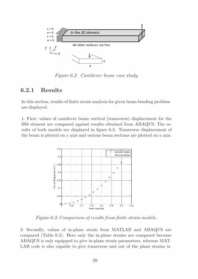
Figure 6.3: Comparison of results from finite strain models.

2- Secondly, values of in-plane strain from MATLAB and ABAQUS arecompared (Table 6.2). Here only the in-plane strains are compared becauseABAQUS is only equipped to give in-plane strain parameters, whereas MAT-LAB code is also capable to give transverse and out of the plane strains in

39

Figure 6.2: Cantilever beam case tudy

6.2.1 Results

In this section, results of finite strain analysis for given beam bending problemare displayed.

1- First, values of cantilever beam vertical (transverse) displacement for theSS8 element are compared against results obtained from ABAQUS. The re-sults of both models are displayed in figure 6.3. Transverse displacement ofthe beam is plotted on y axis and various beam sections are plotted on x axis.

40

Strain Parameter Results from ABAQUS Results from MATLABExx 9.09E-2 8.98E-2Eyy 1.603E-2 1.58E-2Exy 7.278E-3 7.211E-3

output. Deformed and undeformed states of beam obtained from both modelsare illustrated in fig. 6.4.

Table 6.2: Comparison of strain values of finite strain model fromABAQUS and MATLAB.

Figure 6.4: Deformed and undeformed beam geometry obtainedfrom ABAQUS and MATLAB

6.2.2 DiscussionThe vertical tip displacement values obtained from ABAQUS and MATLABare 0.26338 m and 0.261 m respectively. The relative percentage differenceerror is 0.9%. When strain values are compared as shown in table 6.2, a relativepercentage error of 0.92% is obtained. This study proves that SS8 elementexhibits an accurate transverse response when compared with 8 nodecontinuum shell element of ABAQUS.

As described in chapter 2, in case of thin beams, transverse shear strains arenegligibly small however locking can give rise to shear strains consequently

increasing the stiffness of the beam. In this study, SS8 element is used toanalyse beam with Length

T hickness = 30, 300 and 3000 and compared results withan 8 node brick element in ABAQUS to prove that EAS modified element isfree of shear locking. To compensate the reduction of beam’s stiffness in thisanalysis, tip load is reduced by 1000 when thickness is decreased by a factor of10. Results of this comparison are outlined in table 6.3.

Table 6.3: Analysis of thin beam.

41

Length tothicknessratio.

wmax fromcontin-uum shellelement[m].

wmax fromSS8 [m].

wmax frombrick ele-ment [m].

Percentageerror be-tweencolumn 3and 4.

30(thickbeam)

2.14E-1 2.123E-1 2.047E-1 3.58%

300 2.242E-1 2.198E-1 1.783E-1 20.47%3000(thinbeam)

2.26E-1 2.19E-1 1.274E-1 43.46%

6.3.1 Conclusion

It can be seen that brick elements show a sizeable increase in beam stiffness inthin beam case as opposed to SS8 element, whose bending stiffness does notchange much with increasing L/t ratio. For brick element the value of stiffnessincreases from 3.58% to 43.46% as L/t ratio is increased. The reason of thisincrease in stiffness is that 8 node brick elements does not involve modificationssuch as ANS and EAS in its formulation. Hence in case of thin structures, theycannot counter locking phenomenas. Whereas, formulation of SS8 elementinvolves modifications that counter locking. Hence, this analysis indicates thatSS8 element is free of shear locking.

6.4 Cook’s Membrane Problem

The formulated element has been tested with Cook’s membrane problem. Thenature of the problem in Cook’s membrane is shown in fig. 6.5. A skewed plateis cantilevered and subjected to in plane shear load. The material behavioris modelled as isotropic linear elastic with Young’s modulus E = 1 and

42

Figure 6.5: Cook’s membrane study.

6.4.1 Results

For the given shear load and geometric properties, analysis has been carriedout for finite strain models of ABAQUS and MATLAB. A maximum tipdisplacement is measured to be 1.504 units and 1.491 units obtained fromABAQUS and MATLAB respectively. A graph representing mesh conver-gence for the given problem is presented in fig. 6.6. Behavior of SS8 element forvalues of Poisson ratio 0.4, 0.495 and 0.4995 are plotted and displayed in fig.6.7. Deformed state of the skewed membrane obtained from ABAQUS andMATLAB are shown in the figure 6.8.

Poisson’s ratio = The beam is fixed at the left end and subjected to a shearforce F distributed uniformly over right edge of the plate. This testis used to check the presence of membrane locking in an element. In orderto check the elements behavior under Poisson locking, same analysis iscarried out with Poisson ration v = 0.4, 0.495 and 0.4995.

Figure 6.6: Mesh Convergence test for Cook’s membraneproblem at oisson ratio=1/3.

Figure 6.8: Results of Cook’s membrane problem carried out at veryfine mesh.

43

Figure 6.7: Response of Cook’s membrane at different oisson ratios.

u1 = (x +y

2) × 10−3, u2 = (y +

x

2) × 10−3, u3 = 0.0 (6.1)

Mesh description is shown in fig. 6.9.

Figure 6.9: Element mesh for patch test [35].

44

6.4.2 Discussion

This reasonable agreement in value of maximum vertical displacement showsthe membrane response is well captured by SS8 element and there isno membrane locking. It can be seen in g. 6.7 that SS8 element givesan accurate membrane response until v = 0.495. But for 0.4995,SS8 element fails to converge. Hence SS8 element cannot modelresponse of material with Poisson ratio greater than 0.495. Moreover, meshconvergence test shows that 8 node continuum shell element convergesfaster than SS8 element.

6.5 Patch TestIn this section, SS8 is evaluated in context of patch test. Patch check isused to verify if given element is able to fulfil the condition of compatibility,convergence and completeness in finite element analysis. Problem descriptionof this case study is illustrated in fig. 6.9. Material behavior is modelled withE = 10E6 and v = 0.25. Following essential boundary conditions are applied atexterior nodes.

6.5.1 Result

As a result of subjected boundary conditions, the plate undergoes deformationand nodal displacements outlined in table 6.4 are obtained.

Table 6.4: Nodal degrees of freedom in patch test.

Nodal dis-placements

u v u v u v u v

Analyticalsolution

5E-5 4E-5 1.95E-4

1.2E-4

2.E-4 1.6E-4

1.2E-4

1.2E-4

Solutionobtainedfrom SS8elements

4.99E-5

3.9E-5

1.94E-4

1.19E-1

1.99E-4

1.599E-4

1.199E-4

1.2E-4

Moreover, a constant stress state is achieved in all five elements .

S11 = S22 = 1499, S12 = 399.8 (6.2)

45

6.5.2 Discussion

Nodal displacements show a reasonable agreement with analytical formulation [1]. Moreover, constant stress shows that SS8 element has passed the patch test. This should be seen as no surprise since in chapter 3 it was assumed that volume integration of enhanced strain displacement matrix is zero, which is necessary condition for passing the patch test.

6.6 Distortion test

In this case study, in-plane shear locking with respect to mesh distortion isinvestigated. A cantilever beam with length = 10 units and width = height =2units is modeled with finite elements and is subjected to a couple force F = 10at its free end as shown in fig. 6.10. Material is used with Elasticity modulusE= 1.5E3 and oisson ratio v = 0. The distortion in mesh is defined by theparameter s as shown in fig. 6.10.

46

Figure 6.10: Illustration of mesh distortion study.

6.6.1 ResultsAnalytical maximum vertical beam deflection is 1 unit [35]. From MATLAB,maximum vertical deflection is found to be 0.99978 unit. Moreover a dis-tortion sensitivity analysis is carried out as shown in fig. 6.11 and resultsare compared with results obtained from 8 node continuum shell element inABAQUS. In mesh sensitivity analysis, beam is divided in 10 elements, eachwith a length of 1 unit. Therefore value of s is only varied between 0 to 0.5.

6.6.2 Discussion

Maximum vertical displacement obtained from MATLAB matches the ana-lytical result. As value of distortion parameter s is increased, a significant dropis value of vertical displacement is observed. This trend is in similar lines withthe trend obtained by doing the same study in ABAQUS. But from the fig. 6.11it should be noted that SS8 element is is slightly less sensitive to meshdistortion compared to continuum shell element of ABAQUS.

47

1- Beam subjected to end loading: In this study cantilever beam is sub-jected to a tip load and its response in terms of vertical displacement andin-plane strain is compared with ABAQUS. Comparison shows a small rel-ative error of less than 1%, verifying accurate transverse response of SS8element.

2- Analysis of Thin Beam: This study is carried out to assess SS8 ele-ment’s response under shear locking. Results of SS8 elements are comparedwith 8 node hexahedral brick element in ABAQUS. It is observed that brick

48

Conclusion andRecommendationsIn this chapter the results of this research project will be summarized andpotential follow up avenues of research will be explored.

7.1 Conclusion

In this work, an eight node shell element has been formulated using AssumedNatural Strain (ANS) and Enhanced Assumed Strain (EAS) technique. Thisformulation is extended to incorporate geometric and material non-linearityusing Total Lagrangian approach based on constitutive relations of isotropichyper-elasticity. Later this finite strain formulation is verified for intendedresponse by using case studies comprising: 1- A cantilever beam/platesubjected to end loading. 2- Cook’s membrane problem. 3- Patch test. 4- Meshdistortion test. Results are compared against a Neo-Hookean hyper-elasticfinite strain model developed in ABAQUS involving 8 node continuum shellelement. Following conclusions are obtained from these studies.

element shows a stiff behaviour as length to thickness ratio is increased. Whenlength to thickness ratio is increased from 30 to 3000, stiffness of brick ele-ment increases from 3.58% to 43.46%. On contrary to brick element, SS8element retains its stiffness with increase in length to thickness ratio. Thisstudy shows that that SS8 element doesn’t show any extraneous locking inthin structures when subjected to transverse loading.

Cook’s Membrane Problem: This study constitutes a skewed beamsubjected to an in-plane shear load. Accurate membrane response of theskewed beam estimated by SS8 element proves that SS8 element is free ofmembrane locking. Whereas, oisson locking test revealed that SS8 elementdoes not converge for materials with oisson ratio greater than 0.495, thusfailing the oisson locking test. Mesh convergence of Cook’s membrane studyshows that SS8 element exhibits slow convergence when compared with 8 nodecontinuum shell element in ABAQUS

In above mentioned studies, error ranging from 0.5%-1.8% are observed.These errors can be attributed to the difference of element model used inABAQUS and SS8 formulation, explained as follow.

1- In ABAQUS, reduced integration has been carried out coupled with hourglass mode remedies in order to remove shear locking from the continuumshell element. While in SS8 element, ANS and EAS approach has been car-ried out for this purpose.

2- In ABAQUS, the continuum shell element is capable to exhibit 6 degreesof freedom (3 translational DOF and 3 rotational DOF) per node while SS8

49

4- Patch Test: Patch test has been carried out to check quality of formu-lated SS8 element. Patch check is used to verify if given element is able tofulfil the conditions of compatibility, convergence and completeness in finiteelement analysis. In the study, it is shown that a plate with irregular mesh ofSS8 element exhibits constant stress field under given displacement boundaryconditions, which is a necessary condition to pass the patch test.

5- Mesh Distortion Test: In this study a cantilever beam is subjected tocouple force and its tip displacement response is checked by increasing thedistortion parameter s of the mesh. It is observed that value of tip verticaldisplacement of the beam significantly decreases as distortion parameter s isincreased from 0 to 0.49. This trend is compared and verified against resultsof continuum shell element in ABAQUS.

7.3 Future Work

For future work, following recommendations are proposed.

1- The methodology proposed for developing SS8 element can be used todevelop a higher order 20 node element, as the one shown in fig.7.1. It is learntfrom the literature review that by far such element has not been developedmainly because of lack of its application. Mostly in structural analysis usingmore elements with less number of nodes is favoured than using less higherorder elements. In opinion of our research team, 20 node thick shell element isvery feasible for simulating composite manufacturing procedures like vacuuminfusion where linear pressure field [34] is only possible if displacement fieldis quadratic or higher order. Developing such an element will take morecomputation but essentially the same methodology.

50

is only capable of exhibiting 3 degrees of freedom per node. This indicates adifference in respective formulations of SS8 and continuum shell element.

3- The nature of model used in ABAQUS for 8 node continuum shell elementcould not be explored indepth because of the lack of a detailed description inABAQUS theory manual [33].

7.2 Learning outcomes

In this project following learning outcomes and goals have been achieved.

1- An in-house code consisting of 8 node solid shell element is developed,which is capable to capture finite strain and material non-linearity.

2- A great deal of learning in fields of non-linear continuum mechanics andfinite element analysis is achieved.

3- In-depth experience of structured programming in MATLAB.

4- Exposure to Latex, as the documentation of this research project is carriedout in Latex.

Numerical Example ChallengeStretching of a cylinder withfree ends.

Geometric non-linear be-haviour of the elementagainst bending and mem-brane modes.

Bending patch test. Ability of the element to re-produce a constant bending.

Twisted beam. Performance of wrappedstructures when curvaturelocking is dominant.

Compression of Clampedsquare plate.

Studying element’s responseunder buckling.

51

Figure 7.1: 20 node solid shell element

2- In this study, SS8 element is only verified to be free of shear and membranelocking. Membrane and shear locking are most dominant of all lockings whileless dominant lockings such as curvature, thickness and curvature lockingsare yet to be verified. Some case studies that can further verify SS8 element,are proposed in table 7.1.

5

References

1. Mohammad Reza Mostafa, (2011), A geometric nonlinear solid-shell el-ement based on ANDES, ANS and EAS concepts. Unpublished doctoraldissertation, University of Colorado, Boulder.

2. Voyiadjis, George Z., and Dimitrios Karamanlidis, eds., (2013) Advancesin the Theory of Plates and Shells. Elsevier.

3. Arnold, Douglas N., Alexandre L. Madureira, and Sheng Zhang, (2002),On the range of applicability of the Reissner–Mindlin and Kirchho–Love platebending models, Journal of elasticity and the physical science of solids, Vol.67, No. 3, Pg.171-185.

4. Bucalem, M. L., and K. J. Bathe, (1997), Finite element analysis of shellstructures. Archives of Computational Methods in Engineering Vol.4, No.1,Pg.3-61.

5. Wall, Wolfgang A., Michael Gee, and Ekkehard Ramm, (2000), The chal-lenge of a three–dimensional shell formulation the conditioning problem, InProceedings of ECCM, Vol. 99.

6. Alves de Sousa, R. J., R. M. Natal Jorge, R. A. Fontes Valente, and J. M.A. César de Sá., (2003), A new volumetric and shear locking-free 3D enhancedstrain element, Engineering Computations, Vol.20, No. 7, Pg. 896-925.

7. De Sousa, RJ Alves, J. W. Yoon, R. P. R. Cardoso, RA Fontes Valente, andJ. J. Grácio. (2007), On the use of a reduced enhanced solid-shell (RESS) ele-ment for sheet forming simulations, International Journal of Plasticity, Vol.23,No. 3, Pg. 490-515.

8. Andelnger, U., and E. Ramm, (1993), EAS elements for two dimensional,three dimensional, plate and shell structures and their equivalence to HR el-

5

ements, International Journal for Numerical Methods in Engineering, Vol.36,No. 8, Pg.1311-1337.

9. Park, K. C., and G. M. Stanley, (1986), A curved Co shell element basedon assumed natural-coordinate strains, Journal of applied Mechanics, Vol.53,No. 2, Pg.278-290.

10. Cardoso, Rui PR, and Jeong Whan Yoon, (2005), One point quadratureshell element with through-thickness stretch, Computer Methods in AppliedMechanics and Engineering, Vol.194, No. 9, Pg.1161-1199.

11. Cardoso, Rui PR, Jeong Whan Yoon, and Robertt A. Fontes Valente,(2006),A new approach to reduce membrane and transverse shear locking for one-point quadrature shell elements: linear formulation, International Journal forNumerical Methods in Engineering, Vol.66, No. 2, Pg.214-249.

12. Cardoso, Rui PR, Jeong-Whan Yoon, José J. Grácio, Frédéric Barlat, andJosé MA César de Sá, (2002), Development of a one point quadrature shellelement for nonlinear applications with contact and anisotropy, Computermethods in applied mechanics and engineering, Vol.191, No. 45, Pg.5177-5206.

13. Cardoso, Rui PR, and Jeong-Whan Yoon, (2007), One point quadratureshell elements: a study on convergence and patch tests, Computational Me-chanics, Vol. 40, No. 5, Pg.871-883.

14. Cardoso, Rui PR, Jeong Whan Yoon, Made Mahardika, S. Choudhry, R.J. Alves de Sousa, and R. A. Fontes Valente, (2008), Enhanced assumed strain(EAS) and assumed natural strain (ANS) methods for one-point quadraturesolid-shell elements, International Journal for Numerical Methods in Engi-neering, Vol. 75, No. 2, Pg.156-187.

15. Simo, Juan C., and M. S. Rifai, (1990), A class of mixed assumed strainmethods and the method of incompatible modes, International Journal forNumerical Methods in Engineering, Vol.29, No. 8, Pg.1595-1638.

16. Nelvio Dal Cortivo, Carlos A. Felippa, Henri Bavestrello, and William T.M. Silva, (2009), Plastic buckling and collapse of thin shell structures, usinglayered plastic modeling and co-rotational ANDES finite elements, ComputerMethods in Applied Mechanical and Engineering, Vol.198, No5-8, Pg.785-798.

5

17. M. Schwarze and S. Reese. (2009), A reduced integration solid-shell finiteelement based on the EAS and the ANS concept-Geometrically linear prob-lems, International Journal for Numerical Methods in Engineering, Vol. 80,No. 10, Pg. 1322-1355.

18. F. Abed-Meraim and A. Combescure (2002), SHB8PS-a new adaptative,assumed-strain continuum mechanics shell element for impact analysis, Com-puters and Structures, Vol. 80, Pg. 791-803.

19. Farid Abed-Meraim and Alain Combescure (2009), An improved assumedstrain solid-shell element formulation with physical stabilization for geomet-ric non-linear applications and elastic-plastic stability analysis, InternationalJournal for Numerical Methods in Engineering, Vol. 80, No. 13, Pg. 1640-1686.

20. Coultate, John K., Colin HJ Fox, Stewart McWilliam, and Alan R.Malvern, (2008), Application of optimal and robust design methods to aMEMS accelerometer, Sensors and Actuators A: Physical, Vol.142, No. 1,Pg.88-96.

21. Criseld, M-A, (1981), A fast incremental/iterative solution procedure thathandles “snap-through”, Computers Structures Vol.13, No. 1, Pg.55-62.

22. Criseld, M. A., and G. F. Moita, (1980), A COROTATIONAL FORMU-LATION FOR 2D CONTINUA INCLUDING INCOMPATIBLE MODES,International Journal for Numerical Methods in Engineering, Vol.39, No. 15,Pg. 2619-2633.

23. P. G. Bergan, (1980), Finite elements based on energy orthogonal func-tions, International Journal for Numerical Methods in Engineering, Vol.15,No.10, Pg.1541-1555.

24. Bergan, P. G., and M. K. Nygård, (1984), Finite elements with increasedfreedom in choosing shape functions, International Journal for NumericalMethods in Engineering, Vol.20, No. 4, Pg. 643-663.

25. Felippa, C. A., and K. C. Park, (2002), Fitting strains and displacementsby minimizing dislocation energy, In Proceedings of the Sixth InternationalConference on Computational Structures Technology, Prague, Czech Repub-lic, Pg. 49-51.

5

26. De Sá, César, M. A. José, Renato M. Natal Jorge, Robertt A. FontesValente Pedro M.Almeida Areias, (2002), Development of shear locking freeshell elements using an enhanced assumed strain formulation, InternationalJournal for Numerical Methods in Engineering, Vol.53, No. 7, Pg.1721-1750.

27. Quak, Wouter, (2007), A solid-shell element for use in sheet deformationprocesses and the EAS method.

28. Schwarze, Marco, and Stefanie Reese, (2009), A reduced integration solid-shell finite element based on the EAS and the ANS concept—Geometricallylinear problems, International Journal for Numerical Methods in Engineering,Vol.80, No. 10, Pg.1322-1355.

29. Cardoso, Rui PR, Jeong Whan Yoon, Made Mahardika, S. Choudhry, R.J. Alves de Sousa, and R. A. Fontes Valente, (2008), Enhanced assumed strain(EAS) and assumed natural strain (ANS) methods for onepoint quadraturesolidshell elements, International Journal for Numerical Methods in Engineer-ing, Vol. 75, No. 2, Pg. 156-187.

30. Ragnar Larsen, (1997), MULTIPLICATIVE FINITE STRAIN HYPERELASTO—PLASTICITY — Basic Theory and its Relation to NumericalMethodology.

31. Bathe, K. J., Ramm, E., Wilson, E. L. (1975), Finite element formulationsfor large deformation dynamic analysis, International Journal for NumericalMethods in Engineering, Vol.9, No. 2, Pg.353-386.

32. RD Cook, DS. Malkus, and ME. Plesha. Concepts and applications offinite element analysis. John Wiley and Sons, New York, 3rd edition, 1989.

33. Systèmes, D. (2012), ABAQUS 6.12 Theory manual, Dassault SystèmesSimulia Corp., Providence, Rhode Island.

34. Mohammad S. Rouhi (2007), Infusion Modeling Using Two Phase PorousMedia Theory, Independent Master’s Thesis in Solid and Fluid Mechanics,Chalmers University of Technology, Göteborg, Sweden.

35. Klinkel, S., Gruttmann, F., Wagner, W. (2006), A robust non-linear solidshell element based on a mixed variational formulation, Computer Methodsin Applied Mechanics and Engineering, Vol.195, No. 1, Pg.179-201.

5

36. Bathe, K. J. (2006), Finite element procedures, Klaus-Jurgen Bathe,Prentice Hall, Pearson Education, Inc. ISBN: 978-0-9790049-0-2.

37. Klinkel, S., Wagner, W. (1997), A geometrical non-linear brick elementbased on the EAS-method, International Journal for Numerical Methods inEngineering, Vol. 40, No. 24, Pg. 4529-4545.

38. Quy, N. D., Matzenmiller, A. (2008), A solid-shell element with enhancedassumed strains for higher order shear deformations in laminates Tech. Mech,Vol. 28, No. (3-4), Pg. 334-355.

5

Appendix

9.1 Appendix A: Flow Diagram

The related codes in our routines regarding Newton iteration read as below:%

%=============== ==== = MAIN FEM ANALYSIS PROCEDUR ======================================

%

% w Nodal displacements. Let w-i^a be ith displacement component

% at jth node.

% dw Correction to nodal displacements. Let w_i^a be ith displacement

% Component at jth node. Then dofs (w_1^1, w_2^1, w_3^1, w_1^2, w_2^2,

% K Global stiffness matrix. Stored as [K_1111 K_1112 K_1121 K_1122…

% K_1211 K_1212 K_1221 K_1222…

% K_2111 K_2112 K_2121 K_2122…]

%

% F

%

% R

% b

Force vector. Currently only includes contribution from tractions

acting on element faces (i.e. body forces are neglected)

Volume contribution to residual

RHS of equation system

%

clear all; clc;

% Run preproc routine

preproc;

%

dw = zeros (nnode*ndof,1);dw=sparse(dw);

w = zeros (nnode*ndof,1);w=sparse(w);

K= zeros (nnode*ndof,nnode*ndof);K=sparse(K);

R= zeros (nnode*ndof,1);R=sparse(R);

b= zeros (nnode*ndof,1);b=sparse(b);

5

9.2 Appendix B: MATLAB Code

%

% Here we specify how the Newton Raphson iteration should run

% Load is applied in nsteps increments;

% tol is the tolerance used in checking Newton-Raphson convergence

% maxit is the max no. Newton-Raphson iterations

% relax is the relaxation factor (Set to 1 unless big convergence problems)

%

Nsteps = 25;

tol = 0.0001;

maxit = 200;

relax = 1.;

for step=1 : nsteps

loadfactor = step/nsteps;

err1 = 1 . ;

err2 = 1 . ;

nit = 0;

disp(‘%%%%%%%%%%%%%%%%%%%%%%%%%%%%%%%%%%%%%%%%%%%%%%%%%%%%%%%%%%%%%%%%%%%’)

disp(‘%%%%%%%%%%%%%%%%%%%%%%%%%%%%%%%%%%%%%%%%%%%%%%%%%%%%%%%%%%%%%%%%%%%’)

disp(‘%%%%%%%%%%%%%%%%%%%%%%%%%%%%%%%%%%%%%%%%%%%%%%%%%%%%%%%%%%%%%%%%%%%’)

disp (‘%%%%%%%%%%%%%%%%%%% Step Load %%%%%%%%%%%%%%%%%%%%%%%%%%%%%%%’)

disp ([step loadfactor])

disp(‘%%%%%%%%%%%%%%%%%%%%%%%%%%%%%%%%%%%%%%%%%%%%%%%%%%%%%%%%%%%%%%%%%%’)

disp(‘%%%% %%%%%%%%%%%%%%%%%%%%%%%%%%%%%%%%%%%%%%%%%%%%%%%%%%%%%%%%%%’)

disp(‘%%%%%%%%%%%%%% %%%%%%%%%%%%%%%%%%%%%%%%%%%%%%%%%%%%%%%%%%%%%%%%%%%’)

while (err2>tol) & (nit<maxit)

nit = nit + 1;

%Calculate the Global Stiffness Matrix

5

K = globalstiffness (nrecord, ndof, nnode, cords, …

nelem, maxnodes, nelnodes, connect, materialprops, w);

%Calculate global traction vector

F = globaltraction (nol2, py, ivno, nnode);

%Calculate global residual vector

R = globalresidual (nrecord, ndof, nnode, cords, …

nelem, maxnodes, nelnodes, connect, materialprops, w);

%out of balance vector

for n=1 : nnode*ndof

b(n) = loadfactor*F(n) – R(n) ;

end

for n = 1 : nfix

rw = ndof* (fixnodes (1,n)-1) + fixnodes (2,n) ;

for cl=1 : ndof*nnode ;

K (rw,cl) = 0 ;

end

% Solve for the correction

dw = (K\b) ;

% Check Convergence

err1 = 0 ;

err2 = 0 ;

wnorm = 0 ;

for n=1 : ndof*nnode

w(n) = w(n) + relax*dw (n) ;

wnorm = wnorm + w(n)*w(n) ;

err1 = err1+dw (n)*dw (n) ;

err2 = err2+b(n)*b(n); end

% Store traction and displacement for plotting later end

% Run post processing routine plot_disp;

School of Engineering, Department of Mechanical Engineering Blekinge Institute of Technology SE-371 79 Karlskrona, SWEDEN

Telephone: E-mail:

+46 455-38 50 00 info@bth.se