a continuous real-time interactive basin simulator (ribs)
TRANSCRIPT

A Continuous Real-Time Interactive Basin Simulator
(RIBS)by
Valeri Yuryevich Ivanov
Submitted to the Department of Civil and Environmental Engineeringin partial fulfillment of the requirements for the degree of
Master of Science in Civil and Environmental Engineering
at the
MASSACHUSETTS INSTITUTE OF TECHNOLOGY
June 2002
@ Massachusetts Institute of Technology, 2002. All Rights Reserved.
A u th or ............................................................................................................Department of Civil and Environmental Engineering
June, 2002
C ertified by ....................... .....................................Rafael L. Bras
Bacardi and Stockholm Water Foundations Professor,Department of Civil and Environmental Engineering
Thesis Supervisor
Accepted by ........... .. . ......................... '".........................Oral Buyukozturk
Chairman, Departmental Committee on Graduate StudiesSSCHUSETTS INSTITUTE Department of Civil and Environmental Engineering
OF TE~lILLLCNBLOGY
JUN 3 2002
LIBRARIESARCHIVES
MA

--q

A Continuous Real-Time Interactive Basin Simulator
(RIBS)
by
Valeri Yuryevich Ivanov
Submitted to the Department of Civil and Environmental Engineeringon May 9, 2002, in partial fulfillment of the
requirements for the degree ofMaster of Science in Civil and Environmental Engineering
Abstract
This thesis presents enhancements to a rainfall-runoff, event-based model, the Real-TimeInteractive Basin Simulator (RIBS). Major modifications are made in the description ofinfiltration and subsurface saturated lateral exchange processes. The infiltration model isrevised to include a modified Green-Ampt scheme which allows one to account for the cap-illary effects during infiltration in a soil that has exponential decay of the saturated conduc-tivity with depth. A soil moisture redistribution scheme is incorporated in the model toprovide a way of simulating the dynamics of the soil moisture profile during interstormperiods. Also added is the capability of modeling the processes of lateral moisture transferin the ground water system. An unsaturated zone - ground water coupling mechanism isimplemented to account for interdependences between the two systems. All these newlyadded features ensure the capability of the model in applications over longer periods of timeunder a broader range of meteorological conditions.
Another aspect of the presented work is estimation of the basin state at the beginningof a storm. A new soil moisture initialization scheme is implemented which is differentfrom the kinematic parameterization of the soil water profile used in the previous version ofthe model. The initial soil moisture profile is linked to the position of the saturated zone.An independent algorithm is developed that obtains the spatial distribution of the depth tothe water table in a basin based on a steady state assumption of the topography controlledground water.
This thesis presents simulations that test each of the model components. Variousinfiltration events are used to illustrate the sub-grid pixel behavior corresponding to pondedinfiltration and infiltration under conditions of rainfall with constant and variable intensity.The ground water simulations are compared with the 2-D analytical solutions of a linearizedform of the Boussinesq's equation. The overall model performance is demonstrated inapplications for an artificial 1-D hillslope model and a natural watershed. These tests showthe model's capability to simulate the principal phases of hydrologic response of a systemthat couples the unsaturated zone and ground water. Overall, the presented simulationresults are physically sound and encouraging.
Thesis Supervisor: Rafael L. BrasTitle: Bacardi and Stockholm Water Foundations Professor


Acknowledgments
I gratefully acknowledge the National Aeronatics and Space Administration (NASA) andthe Department of Civil and Environmental Engineering for the financial support of thiswork.
I am particularly grateful for the continued guidance and support of my advisorRafael Bras who has been coaching me all that time spent at MIT. I thank Dara Entekhabiwho provided valuable suggestions and assistance throughout the work. I am grateful topeople from Parsons Lab, its current "residents" and alumni, whose work and advice helpedin completing this thesis. Special acknowledgements deserve Scott Rybarczyk, EnriqueVivoni, Nicole Gasparini, Greg Tucker, Jingfeng Wang, Vanessa Teles, Jean Fitzmaurice,Frederic Chagnon, and Daniel Collins. I would like to thank Luis Garrote and MarizaCabral who I have never had a chance to meet. I am very much grateful to the Departmentof Hydrology at Moscow State University where I spent wonderful years "learning rivers",my former advisor Victor Zhuk in particular. Lastly, special words of gratitude deserve myfamily and my wife Tatyana.

Eu

Contents
I Intoduction 13
1.1 Introduction, motivation, and scope of the work ................................. 13
1.2 R elevant literature ................................................................................ 16
II Core Model and Its Modifications 23
2.1 Infiltration and runoff generation scheme ............................................ 23
2.1.1 Basin representation .................................................................... 23
2.1.2 Runoff generation ....................................................................... 25- Basic Assumptions ..................................................................... 25- Infiltration Model Description .................................................... 28
Saturated infiltration ......................................................... 30Unsaturated infiltration ..................................................... 32Evolution of fronts ............................................................ 37
- Subsurface flow exchange .......................................................... 39- Runoff generation schematic ...................................................... 41
2.1.3 Surface flow routing scheme ....................................................... 44
2.2 Transformation to a continuous operation .......................................... 47
2.2.1 Soil water redistribution and subtraction..................................... 48
2.2.2 Coupling procedure between fronts of the unsaturated zone andw ater tab le ............................................................................................ 53
2.3 Ground water model description ......................................................... 54
2.3.1 Formulation of the ground water model ...................................... 54
2.3.2 Ground water flow partitioning ................................................... 57
2.4 Modifications of the ground water module allowing continuousoperation .................................................................................................... 6 1
III Initialization Schemes 71
3.1 Fixing the water table depth: overview of strategies and a modifiedapproach of steady-state ground water distribution ................................... 71
3.2 An overview of soil moisture initialization schemes. Hydrostaticequilibrium moisture profile ...................................................................... 77
IV Model Performance: Synthetic Off-line Tests 87
4.1 Test case: ponded infiltration into a semi-infinite soil column ............ 87
4.2 Test case: rainfall of constant and variable intensity ........................... 93
- 'III
4.3 Ground water model off-line testing ..................................................... 101
4.3.1 Damping of a ground water mound in the infinite plane ............. 101
4.3.2 Instantaneous filling of a canal: semi-infinite case ...................... 108
V Model Performance: On-line Model Applications 113
5.1 Test case: the hillslope model ............................................................... 113
5.1.1 T he w et case ................................................................................. 1 14
5.1.2 T he dry case.................................................................................. 1 19
5.2 Test case: Peacheater Creek Basin ........................................................ 131
VI Conclusions 141
6.1 Summary of development and implementation results ......................... 141
6.2 Summary of simulation results ............................................................. 143
Appendix 1
The Green-Ampt model for non-uniform soils. Formulation of the wet-ting front capillary drive ............................................................................. 145
Appendix 2
Formulation of the wetting front capillary drive for the unsaturated infil-tration case .................................................................................................. 15 7
Appendix 3
Derivation of an equation for evolution of the top front of the perched sat-urated zon e ................................................................................................. 159
Appendix 4
Derivation of an equation for the water table depth given the soil moistured eficit .......................................................................................................... 16 3
Appendix 5
Subtraction and addition of moisture above/below the wetting front in the
perched saturated zone ............................................................................... 165
Bibliography 167
List of Figures
2.1 RIBS representation of a subgrid element ............................................. 24
2.2 Schematic representation of the computational element verticalstructure w ithin the RIB S ....................................................................... 32
2.3 Schematic representation of the computational element in theunsaturated zone .................................................................................... 36
2.4 Four basic pixel states: Unsaturated, Perched Saturated, SurfaceSaturated, and Fully Saturated ............................................................... 44
2.5 Schematic representation of a flow path for a hillslope node ................. 46
2.6 Illustration of the module estimating water table drop from the soilsurface ................................................................................................ .... 4 9
2.7 Illustration of the module computing water table drop in a cell havinginitial ground water level at some depth below the soil surface ............. 50
2.8 Illustration of the basic drying cycle ...................................................... 50
2.9 Illustration of direct water table re-adjustment ...................................... 52
2.10 Computation of flow direction on planar triangular facets ..................... 60
2.11 Flow partitioning across edges of rectangular box ................................. 61
2.12 Illustration of the module accounting for the transition into thesaturated state caused by the ground water influx .................................. 62
2.13 Illustration of the module accounting for the water table drop in theunsaturated zone - ground water coupling scheme ................................ 67
2.14 Illustration of the module accounting for the water table rise in theunsaturated zone - ground water coupling scheme. Part I. .................... 68
2.15 Illustration of the module accounting for the water table rise in theunsaturated zone - ground water coupling scheme. Part II. ................... 69
3.1 Groundwater topography before the smoothing procedure ................... 76
3.2 Estimated depth to the water table. Peacheater Creek, OK .................... 77
3.3 Surface soil moisture variation of hydrostatic profile depending ondepth to the water table (soil properties represented by the Brooks-Corey param eterization) ........................................................................ 82
3.4 Surface soil moisture corresponding to the hydrostatic assumption ofpressure distribution in (Touchet silt loam, Brooks-Corey parameter-ization) .............................................................................................. ..... 83

3.5 Soil moisture distribution corresponding to the hydrostatic assumptionin Brooks-Corey soils ............................................................................ 84
4.1 Ponded infiltration: base case ................................................................. 89
4.2 Ponded infiltration: f parameter varied ................................................. 90
4.3 Ponded infiltration: 19b parameter varied .............................................. 91
4.4 Ponded infiltration: shallow water table ................................................. 92
4.5 Simulation of infiltration: constant rainfall of 4 mm/hour intensity ....... 96
4.6 Simulation of infiltration: constant rainfall of 10 mm/hour intensity ..... 97
4.7 Simulation of infiltration: constant rainfall of 20 mm/hour intensity ..... 98
4.8 Simulation of infiltration: rainfall of variable intensity, deep water tableca se ..................................................................................................----... 9 9
4.9 Simulation of infiltration: rainfall of variable intensity, shallow watertab le case ................................................................................................. 10 0
4.10 Ground water mound .............................................................................. 102
4.11 Water table head for simulation run time 50 hours and 240 hours: MSapproach ............................................................................................. 104
4.12 Water table head for simulation run time 50 hours and 240 hours: Dooapp ro ach .................................................................................................. 10 5
4.13 The error surfaces: Hour 50 .................................................................... 106
4.14 The error surfaces: Hour 150 .................................................................. 107
4.15 Water table head for simulation run time 240 hours: both approaches ... 110
4.16 The error surfaces: Hour 50 .................................................................... 111
4.17 The error surfaces: Hour 240 .................................................................. 112
5.1 Representation of an artificial hillslope .................................................. 121
5.2 Cross-sectional view of the hillslope: end of 11-hour 1 mm/hour rain-fall period (w et case) ............................................................................... 122
5.3 Cross-sectional view of the hillslope: end of 18-hour no-rainfall period(w et case) ..................................................................................... . ...... 123
5.4 Cross-sectional view of the hillslope: end of 16-hour 1 mm/hour evap-oration period (wet case) ......................................................................... 124
5.5 Cross-sectional view of the hillslope: end of 14th hour of 16-hour 10mm/hour rainfall event (wet case) ........................................................... 125
5.6 Cross-sectional view of the hillslope: end of 10-hour 3 mm/hour evapo-ration period (w et case) ........................................................................... 126
5.7 Hyetograph and hydrograph for the hillslope simulation (wet case) ...... 127
5.8 Cross-sectional view of the hillslope: end of 14th hour of 16-hour 10mm/hour rainfall event (dry case) ........................................................... 128
5.9 Cross-sectional view of the hillslope: end of 10-hour 3 mm/hour evapo-ration period (dry case) ........................................................................... 129
5.10 Hyetograph and hydrograph for the hillslope simulation (dry case) ....... 130
5.11 Surface topography of the Peacheater Creek watershed ......................... 131
5.12 Summary plot for Peacheater Creek calibration ..................................... 135
5.13 Peacheater Creek: water table at the surface (simulation results) ........... 136
5.14 Peacheater Creek: runoff generation (simulation results) ....................... 137
5.15 Peacheater Creek: subgrid pixel behavior, Case 1 .................................. 138
5.16 Peacheater Creek: subgrid pixel behavior, Case 2 .................................. 139
5.17 Peacheater Creek: subgrid pixel behavior, Case 3 .................................. 140
AL.1 Example of pressure distribution in the saturated thickness ................ 147
Al.2 A sketch of the general and the Green-Ampt soil moisture profiles ....... 149
Al.3 Sensitivity of the capillary drive term to various parameters .................. 155
Al.4 Fit of the model to the data of Childs and Bybordi [1969] ...................... 156
A3.1 An illustration of the domain of interest Q ............................................. 159
A5.1 An illustration of the soil water profile for the perched saturated case ... 165


CHAPTER I
Introduction
1.1 Introduction, motivation, and scope of the work
Within the last decade new distributed data sources have created a real wealth of informa-
tion for hydrologists. Among the major components significant to flood forecasting capa-
bilities was the establishment of the Next Generation Weather Radar (NEXRAD) which
provides radar-generated rainfall maps and facilitates gradual improvement of quantitative
precipitation forecasts (Olson et al., (1995)). Information about geometry, topography and
soil properties of river basins has become readily available from the USGS Digital Eleva-
tion Models (DEM), various soils and land use databases such as the Soil Conservation Ser-
vice (SCS) State Soil Geographic Databases (STATSGO, SSURGO), the USGS Land Use
and Land Cover (LULC) database, and many other local data banks supported by different
scientific communities. The level of detail and precision of this type of information have
undergone considerable re-evaluation and changes (e.g. Farr et al., 2000) in recent years
providing a real wealth of data to flood forecasters. Introduction of these new technologies
calls for the improvement of forecasting skills of rainfall-runoff models by using all avail-
able information describing the spatial heterogeneity of the land surface and hydrometeoro-
logical forcing. Accordingly, recent research efforts in the flood forecasting area have been
focused on distributed hydrologic modeling schemes.
The possibility to include detailed basin information on topography, soil types, veg-
etative cover, and geology and make effective use of radar-generated rainfall estimates is a
promising and attractive opportunity for flood forecasting. Topography has been proven to
affect runoff generation significantly, in particular peak streamflow. The soil type and vege-
tation cover/ land use type may characterize highly permeable top soil horizons or crusty
surface layers that have low water conductivity. The combined effect of accounting for soil
type and land use along with moisture availability allows one to describe different runoff
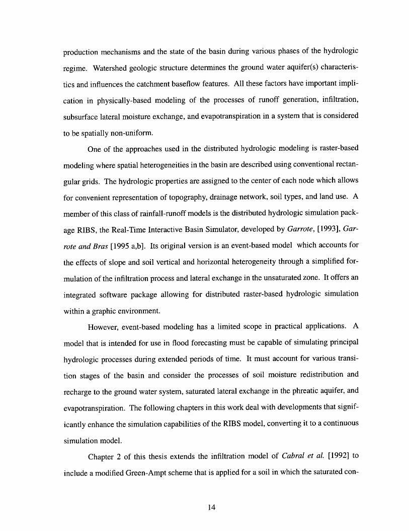
production mechanisms and the state of the basin during various phases of the hydrologic
regime. Watershed geologic structure determines the ground water aquifer(s) characteris-
tics and influences the catchment baseflow features. All these factors have important impli-
cation in physically-based modeling of the processes of runoff generation, infiltration,
subsurface lateral moisture exchange, and evapotranspiration in a system that is considered
to be spatially non-uniform.
One of the approaches used in the distributed hydrologic modeling is raster-based
modeling where spatial heterogeneities in the basin are described using conventional rectan-
gular grids. The hydrologic properties are assigned to the center of each node which allows
for convenient representation of topography, drainage network, soil types, and land use. A
member of this class of rainfall-runoff models is the distributed hydrologic simulation pack-
age RIBS, the Real-Time Interactive Basin Simulator, developed by Garrote, [1993], Gar-
rote and Bras [1995 a,b]. Its original version is an event-based model which accounts for
the effects of slope and soil vertical and horizontal heterogeneity through a simplified for-
mulation of the infiltration process and lateral exchange in the unsaturated zone. It offers an
integrated software package allowing for distributed raster-based hydrologic simulation
within a graphic environment.
However, event-based modeling has a limited scope in practical applications. A
model that is intended for use in flood forecasting must be capable of simulating principal
hydrologic processes during extended periods of time. It must account for various transi-
tion stages of the basin and consider the processes of soil moisture redistribution and
recharge to the ground water system, saturated lateral exchange in the phreatic aquifer, and
evapotranspiration. The following chapters in this work deal with developments that signif-
icantly enhance the simulation capabilities of the RIBS model, converting it to a continuous
simulation model.
Chapter 2 of this thesis extends the infiltration model of Cabral et al. [1992] to
include a modified Green-Ampt scheme that is applied for a soil in which the saturated con-

ductivity exponentially decays with depth. It also supplements the infiltration model with a
soil moisture redistribution scheme that provides a physically reasonable way to mimic the
dynamics of the soil moisture profile during a rainfall hiatus and interstorm periods. A new
parameterization is added that allows for extraction of moisture from a soil water profile,
therefore simulating evaporation conditions. These procedures significantly expand the
range of meteorological conditions under which the model can be used. The model of Gar-
rote [1993], Garrote and Bras [1995 a,b] has also been extended to incorporate a ground
water module that simulates the lateral fluxes in the saturated zone. Chapter 2 also gives a
description of development of an unsaturated zone - ground water coupling scheme that
simulates interaction of moving fronts and changing ground water level. The scheme
ensures the capability of the model in applications over long periods of time.
Chapter 3 deals with the basin initialization models. It provides a general overview
of various approaches for specifying the soil moisture state and ground water level distribu-
tion at the beginning of a simulation. An approach using a steady state assumption of
topography controlled ground water (Sivapalan et al., 1987) is described in more detail. It
is used as a RIBS input procedure to initialize depth to the water table in a basin. The
approximation uses soil hydraulic properties, topography information, and a mean depth to
the water table in a catchment. It is further assumed that location of the ground water level
significantly controls wetness conditions in the basin. Knowledge of the water table depth
is related to the distribution of moisture in the unsaturated zone. The model uses the hydro-
static equilibrium parameterization for the vertical distribution of pressure head which cor-
responds to zero initial flux in the unsaturated zone. The Brooks-Corey parameterization of
soil hydraulic properties defines the corresponding initialization soil moisture profile in the
form of convenient for treatment closed-form expression.
Chapter 4 presents off-line tests of the infiltration model applied to a horizontal lat-
erally infinite soil column in which the saturated conductivity is assumed to decay with
depth. First, a ponded infiltration case is discussed which demonstrates the general validity

of the modified Green-Ampt scheme. Soil response to constant rainfall intensities of vari-
ous magnitude is also simulated. The unsaturated, perched, and surface saturated phases of
infiltration are discussed and the conceptual validity of the model is shown. The simulation
results for a sequence of storm and interstorm periods are also presented which demonstrate
the capability to run the model continuously. Two ground water flow partitioning schemes
considered by the model are compared in this chapter. Analytical solutions for 2-D cases
are used as a benchmark in these simulations.
Chapter 5 applies RIBS to a synthetic one-dimensional hillslope to evaluate how
realistically the model simulates infiltration and subsurface lateral exchange in the unsatur-
ated and saturated zones. The simulation includes rainfall and evaporation periods. The
dynamics of the principal variables is discussed for two cases: initially wet and dry. The
results indicate a general agreement between the model behavior and the expected response
in the hillslope system.
A single calibration example is presented for Peacheater Creek basin in Oklahoma.
The model is applied for an event that includes a storm hiatus and interstorm period. Using
NEXRAD rainfall data the calibration of the simulated streamflow is performed. The fit of
the model output to the observed storm flow is found to be reasonably good, and the cali-
brated parameter values are within a physically reliable range. Several cases of subgrid
model behavior are illustrated for pixels located in different regions of the catchment. They
demonstrate the general consistency of the simulations with hypothesized dynamics in vari-
ous hillslope sections.
This thesis presents a work in progress, and its current conclusions and suggestions
for further investigation are given in Chapter 6.
1.2 Relevant literature
The model development described in the current work covers a rather broad range of topics.
Relevant references are given in this section that are good as general introduction to the

approaches used in the description of hydrologic processes and becoming familiar with the
area of distributed rainfall-runoff modeling. Specific literature references are also given in
the chapters and appendices of this thesis.
Extensive literature exists on infiltration. Philip [1957] presents a detailed analysis
of the theory of flow through unsaturated porous media applied to the problem of infiltra-
tion. Analytical solutions for Richard's equations exist only for unrealistic assumptions
based on the adoption of a uniform soil moisture with depth and constant positive moisture
flux into the soil (e.g. Philip, 1957; Parlange, 1971; Broadbridge and White, 1988; White
and Broadbridge, 1988; Warrick et al., 1990). An exact analytical solution for a continuous
infiltration process within a given storm of variable intensity is not available. Approximate,
physically based approaches for continuous infiltration events have been developed (e.g.
Green and Ampt, 1911; Mein and Larson, 1973; Smith and Parlange, 1978; Parlange et al.,
1982; Smith and Hebbert, 1993; Smith et al., 1993; Corradini, et al., 1994). These approx-
imate approaches extend to variable rainfall rates and some of them account for soil water
redistribution during dry periods (Corradini, et al., 1994; Ogden and Saghafian, 1997).
Skaags and Khaleel [1982] and Singh [1989] provide reviews of conceptual and empirical
infiltration models used to estimate rainfall excess under one-dimensional and lumped
approaches.
The extension of the one-dimensional infiltration problem to the two-dimensional
analysis of flow in a hillslope has also been extensively studied. The vertical infiltration in
this case is combined with the lateral subsurface flow in the unsaturated and saturated
zones. Freeze [1972] made an outstanding study of the dynamics of the hydrologic
response of subsurface process-controlled catchments. His model treats the saturated and
unsaturated regions of soil in a unified two- or three-dimensional flow equation solution
which provides a revealing look at the saturation from below mechanism. Zaslavski and
Sinai [1981 a, b, c] in a series of papers study the effects of soil heterogeneity in a system
consisting of layers of homogeneous isotropic soil with different hydraulic properties. Such

a system behaves as a nonisotropic soil matrix, and they discuss mechanisms that result in
downstream lateral flow parallel to the soil surface. In this matter, they discuss the impor-
tance of the surface "transition layer", a layer that refers to the top portion of the soil having
higher hydraulic conductivity due to macropores. Germann and Beven [1982] stress the
importance of macropores of the soil surface layer in infiltration and subsurface storm flow.
Beven [1982 a, b] presents an analytical model of hillslope subsurface stormflow generation
based on the kinematic wave theory. Smith and Hebbert [1983] introduce a mathematical
model that integrates all the major hydrologic response mechanisms of a simple hillslope to
analyze the relationships between rainfall, soil hydraulic properties, hillslope geometry, and
runoff characteristics. Among the findings is the conclusion that the subsurface stormflow
is highly affected by anisotropy and the spatial distribution of the saturated conductivity.
The vertical growth of the saturated zone is demonstrated to have a potentially greater effect
on runoff than horizontal movement in cases where anisotropy is not high. Philip [1991 a,
b] presents an approach to obtain an infinite-series solution for the full non-linear unsatur-
ated flow equation for a planar, convergent and divergent hillslope. The analysis also
applies to two cases where the soil anisotropy is considered: the principal direction is either
horizontal or parallel to the soil surface. A markedly different behavior is found between the
cases. Philip [1991 c] studies infiltration on convex and concave slopes. He underlines the
dominant role of surface slope in determining the dynamics of infiltration normal to the
slope and the dynamics of downslope unsaturated flow. Kirkby [1978] and Anderson and
Burt [1990] are an excellent reference to reviews of studies in hillslope hydrology.
The saturated zone dynamics are important in terms of both the infiltration process
and runoff generation. Among the best references to the theory of ground water hydraulics
are Bear [1979] and Bear [1972]. The theory of flow through porous media in the unsatur-
ated and saturated phases is given in Bear [1972] who emphasizes understanding the micro-
scopic phenomena occurring in porous media and their implications at a macroscopic scale.
Bear [1979] provides a full review of the mathematical treatment of the ground water flow

problem. He provides a number of approaches to solve the ground water problem either
analytically, numerically, or by means of laboratory models and analogs. Polubarionova-
Kochina [1952] provides a full spectrum of analytical solutions to particular ground water
problems which include one-, two-, and three-dimensional cases. They can be used as a
benchmark while evaluating the performance of a numerical ground water model.
Distributed rainfall-runoff models attempt to consider various processes of the mois-
ture cycle as highly interdependent components of a catchment hydrologic system. They
account for spatial heterogeneity of properties in the simulated domain and link individual
processes to reproduce the interior dynamics of hydrologic variables based on physical
arguments. The area of distributed hydrologic modeling has been in constant evolution for
the last 30-35 years but only in the last 15 years have distributed models been actually
applied to catchments of a quite large scale. Perhaps the pioneering work in distributed
modeling belongs to Freeze and Harlan [1969] and Freeze [1972] who constructed a three-
dimensional model based on the numerical integration of the partial differential equations
governing overland and subsurface flow. Since then, a wide variety of physically based dis-
tributed models have been constructed for the characterization and prediction of watershed
hydrology. Intensive data requirements prevent using fully three-dimensional numerical
schemes and simplifications are usually made to keep the models computationally feasible.
They usually involve reducing the dimensionality of the problem by discretizing the water-
shed into coupled one- or two-dimensional components. Differences in the goals and meth-
ods used by model developers have led to significant diversity between the models. A
relevant review of the topic is given by Abbot and Refsgaard [1996], Singh [1995], DeBarry
et al. [1999]. A short description of some of the models that are or could potentially be
used for flood forecasting purposes is given below.
One of the most widely referenced distributed hydrologic models is the Systeme
Hydrologique Europeen, or SHE model developed by the Danish Hydraulic Institute (Abbot
et al., 1986). SHE is a basin scale model, simulating overland flow, channel flow, saturated

and unsaturated subsurface flow, along with interception, evaporation, and snowmelt.
Hydrologic processes in the SHE model are represented by numerical schemes of various
dimensionality. Channel flow and unsaturated zone subsurface flow are averaged to a single
dimension. Overland flow is calculated in two dimensions. A fully 3-D ground water
model simulates the subsurface flow in the saturated zone. Finite difference method numer-
ical schemes are used to calculate mass and energy conservation on an orthogonal grid net-
work.
The Institute of Hydrology Distributed Model IHDM (Beven et al. 1987) is concep-
tually similar to the SHE model. The model structure places more emphasis on the basin
representation. Rather than following a rectangular grid, the catchment is divided into hill-
slope and channel components of irregular shape but the same basic processes are included
in the simulation framework.
The Cascade of 2-D Planes CASC2D model (Julien and Saghafian, 1991; Ogden,
1997) started as an overland flow algorithm. It was largely expanded later to create a phys-
ically based continuous hydrologic model for flood forecasting. The model is based on a
raster data platform. It includes continuous soil moisture accounting through numerical
solution of the 1-D Richard's equation (Philip, 1957) with inclusion of interception and
evapotranspiration schemes. The dimensionality of the model is 2-D overland flow and 1-D
channel flow. Recent enhancements include development of a 2-D ground water model.
THALES is a set of hydrological modelling modules that subdivides the model area
into interconnected irregular shaped elements and calculates a number of topographic
attributes for each element (Grayson et al., 1995). Each element has uniform infiltration,
surface, and subsurface parameters although they are allowed to vary between different ele-
ments. The model is a relatively simple physics-based model that enables a wide range of
hydrologic processes to be represented through incorporation of the Hortonian mechanism
of surface runoff as well as representation of variable-source-area runoff and exfiltration of
subsurface flow.

Real-Time Interactive Basin Simulator RIBS (Garrote and Bras, 1993) was devel-
oped as a single event raster-based hydrologic model that assumed the dominant role of
topography in basin hydrologic response. It was designed as a flood forecasting tool for
medium- to large-scale watersheds. The model hydrology accounted for the effects of slope
and soil vertical and horizontal heterogeneity through a simplified formulation of the infil-
tration process and lateral exchange in the unsaturated zone. This work modifies the
description of infiltration and subsurface saturated lateral exchange processes, significantly
enhancing simulation capabilities of the model. The most important enhancements concern
the added capability of simulating catchment hydrologic response continuously during
storm and inter-storm periods. RIBS modifications are the subject of this thesis and are
discussed in the following chapters.

CHAPTER II
Core Model and Its Modifications
This chapter describes the RIBS model - Real-Time Integrated Basin Simulator - a distrib-
uted, physically-based rainfall-runoff model that includes a real-time flood forecasting envi-
ronment. The model inherits the structure and logic of the original event-based version
Distributed Basin Simulator (DBS) developed by Garrote [1993] and Cabral et al. [1992].
The discrete spatial representation of terrain based on the raster structure allows one to track
the evolution of moisture waves within a computational element and their redistribution by
the lateral fluxes in the unsaturated zone and in the phreatic aquifer during wetting and dry-
ing periods. The description follows much of the Garrote [1993] and Cabral et al. [1992]
work with the supplements dealing with the continuous simulation capabilities added in this
work.
2.1 Infiltration and runoff generation scheme
2.1.1 Basin representation
The event-based Distributed Basin Simulator is the core of RIBS. It represents the three-
dimensional structure of the basin on a number of data layers which contain two-dimen-
sional information. Using a conventional rectangular grid with the hydrologic properties
assigned to the center of each node allows for efficient representation of topography, drain-
age network, soil types, and land use. Dictated by the base resolution of the Digital Eleva-
tion Model (DEM) data layer, the geometry of each grid cell is represented as a two-
dimensional section of sloped soil (Figure 2.1) on three data layers: elevation, orientation,
and slope. The elevation of the element is defined by the DEM and corresponds to its cen-
tral point. The land surface slope orientation of the element is "discrete" and defined in the
direction of one of the eight surrounding neighbors, in the direction of steepest descent
(approach is often referred as "D8", see Section 2.3). Connectivity between cells is there-

fore described as "drains to" reflecting the aspect relationship between contiguous pixels.
The same single drainage direction is assumed for the vadose zone fluxes implying that the
subsurface moisture exchange is dominated by gravity and enforced by soil anisotropy. The
direction of the ground water flow is defined based on simulated gradients of the ground
water level. Such a coupling scheme at the pixel scale effectively implements large scale
interaction within the basin allowing moisture transfer among computational elements and
subsequent non-linearity in the basin response.
dx
p
dy
Figure 2.1: RIBS representation of a subgrid element
The basin drainage network is obtained from the DEM using the notion of "total
contributing area". For a given grid element this equals the number of pixels whose flow
reaches the pixel of interest following the path of steepest descent, the "D8" methodology
mentioned previously. Assuming a certain threshold for contributing area, pixels with
exceeding values may be considered as a stream. The drainage network can thus be
extracted from the contributing area map. The threshold value is determined such that the
overall drainage density of the computed stream network is approximately equal to the
drainage density of the network obtained from the USGS quadrangle maps.
Two different scales of variability are combined in the model. Large scale horizon-
tal heterogeneity is represented by a mosaic of pedologic and geomorphologic properties on

the nodes of the rectangular grid. Soil data are usually much coarser than the DEM and the
model therefore emphasizes topography as the basis in the analysis of basin response. Each
cell is assumed to have laterally homogeneous properties with several properties assigned to
the node. Some subgrid variability is also considered but only in the normal with respect to
the terrain surface direction. The subgrid analysis is carried out in a reference system
defined by the coordinate system (n, p) (Figure 2.1), where n follows the direction normal to
the terrain slope (positive downward) and p follows the direction parallel to the plane of the
maximum slope (positive downslope). All the variables within the element are assumed
constant in the plane parallel to the land surface and variability is considered only in the
direction n. This will be explained in the following section.
The model was designed to work on grids with any number of elements but the
upper limit is set by hardware limitations: memory allocation and execution time. These
constraints are much more flexible than in the earlier days of DBS implementation. The
execution time however is still an issue considering time step limitation in the explicit
numerical scheme used. Currently, the base resolution most commonly used is the DEM
standard grid spacing, 30 m x 30 m. However larger grid cell sizes can also be used to
increase the model real-time efficiency.
2.1.2 Runoff generation
- Basic Assumptions
The reference system is defined by the axes n and p introduced in the previous section (Fig-
ure 2.1). The model considers a soil column of heterogeneous, anisotropic, and sloped soil
in which the saturated hydraulic conductivity decreases with normal depth. The properties
are assumed constant on a plane perpendicular to the (n, p) plane of a grid cell. The spatial
variability in the domain is considered by the elements of the grid.
Besides accounting for the large scale heterogeneity in the two-dimensional plane,
soils in the model also exhibit non-uniformity with depth. Beven [1982, 1984] argues that
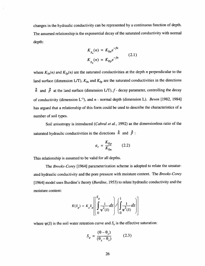
changes in the hydraulic conductivity can be represented by a continuous function of depth.
The assumed relationship is the exponential decay of the saturated conductivity with normal
depth:
K (n) = Kone-f
K (n) = Kopf
where Ksn(n) and Ksp(n) are the saturated conductivities at the depth n perpendicular to the
land surface (dimension L/T), Kon and Ko, are the saturated conductivities in the directions
h and p at the land surface (dimension L/T), f - decay parameter, controlling the decay
of conductivity (dimension L-1), and n - normal depth (dimension L). Beven [1982, 1984]
has argued that a relationship of this form could be used to describe the characteristics of a
number of soil types.
Soil anisotropy is introduced (Cabral et al., 1992) as the dimensionless ratio of the
saturated hydraulic conductivities in the directions n and p:
a,. = (2.2)KOn
This relationship is assumed to be valid for all depths.
The Brooks-Corey [1964] parameterization scheme is adopted to relate the unsatur-
ated hydraulic conductivity and the pore pressure with moisture content. The Brooks-Corey
[1964] model uses Burdine's theory (Burdine, 1953) to relate hydraulic conductivity and the
moisture content:
TSe
K(Se) = Ks e K 2 ds f 21 dV (S M) 0 V (S)
where W(S) is the soil water retention curve and Se is the effective saturation:
Se = 0 (2.3)e(Os - Ord

where Q, is the saturated moisture content (assumed to be equal porosity), and 0 , is the
residual moisture content, defined as is the amount of soil water that cannot be removed
from the soil by drainage or evapotranspiration. Brooks-Corey [1964] used Burdine's the-
ory assuming the empirical model for soil water retention curve:
1
e(S) = VbSe (2.4)
(where 9b is the air entry bubbling pressure and X is the pore-size distribution index) to get
the expression relating unsaturated conductivity and the soil moisture content:
2+3X 2+3X
Kn(Se) = KsSX = K (2.5)SeS
Substitution of Equations 2.1 for the saturated conductivities in the directions h and p
into Equation 2.5 yields:
2+3X0
Kn(0, n) = KonefnS, = KOne 67_7
2+3X (2.6)
K(0, n) = Kope Se = Kpef _ jS r
where Kn and K, are the unsaturated conductivities (dimension L/T: mm/hour) in the direc-
tions n and p at moisture content 0 and depth n. Therefore, given the soil parameters
and the distribution of moisture content (or matric potential) in the vadose zone, the unsat-
urated conductivity is obtained from Equation 2.6. It is worth noting that Kon, Os, and Or are
measurable parameters and thus have physical meaning. Parameter X has more or less obvi-
ous physical sense either being small for media having a wide range of pore sizes or large
for media with a relatively uniform pore size. The parameterization has a limitation: it is
applicable only for the range of yi satisfying y > N'b. It is necessary to note that though the
Brooks-Corey model was developed for isotropic media (drainage cycle, hysterisis
neglected) it appears feasible to apply the model (2.6) for non-uniform soils.

- Infiltration Model Description
The flow vector in the unsaturated zone for sloped soil can be expressed as:
= (0, n) ni - K=(0, n)Ti=
-Kn(O, n)(jy - cosa>,, - KP(O, n)( - sin aP (2.7)
where ah and L are the components of the hydraulic gradient vector in directions A andan a
4
p ; a and LY are the capillary potential gradients respectively; and in and i, are unit
vectors in these directions (cos a and sin a are needed because gravitational forces are
assumed to act along vertical direction).
An exact solution of Equation 2.7 for a continuous infiltration process which
accounts for both the pre-ponding and the post-ponding stages is not available. However,
approximate, physically based descriptions of the infiltration process for simple continuous
operation have been developed. The original RIBS infiltration model is based on the kine-
matic approximation (Beven, 1981, 1982; Charbeneau, 1984) for the flow in the unsaturated
zone. The assumption neglects suction forces and uses the gravitational component as dom-
inant in the infiltration process. Beven [1982] wrote: "...greatly simplified models may be
sufficient to predict the subsurface response to storm rainfall on hillslopes... justification for
this contention is based on the predominance of gravity over capillary forces in controlling
the movement of free water within the soil... for both saturated and unsaturated flows it is
possible to neglect terms involving capillary and pressure potentials and yet retain a useful
predictive model". Indeed, using both the kinematic assumption and expression 2.2, equa-
tion (2.7) conveniently transforms to:
= Kn(, n)cos a -i + K,(0, n)sin c - , =
= K,(On)cosa -i + aK(0, n)sin a -, (2.8)
From the steady-state flow analysis of unsaturated infiltration under constant rainfall rate R
in a uniform slope of infinite length it follows that (Cabral et al., 1992):
K,(0, n) = R (2.9)
which is evident for the kinematic flow assumption. Such an approximation is mostly appli-
cable for later stages of infiltration when a sufficient amount of water has accumulated in
the soil. It is also a plausible assumption for soils having very high hydraulic conductivity
(e.g. sands) relative to the rainfall rates such that there is no control imposed by the soil on
infiltration rates. The original RIBS completely relies on the kinematic approximation and
its full description is given by Garrote [1993].
In many cases, however, ignoring soil suction potential may lead to a substantial
underestimation of the infiltration volume. Eagleson [1970] writes, describing the impor-
tance of suction: "...the gravitational gradient is small with respect to that of capillarity (that
is, L4 >> 1). It has been argued that these conditions are often met when the saturation is
relatively low, such as in the early stages of infiltration and in the later stages of exfiltra-
tion". This note becomes especially important in continuous simulation of rainfall-runoff
process, the case when the wet and the dry soil states are sequential and may have signifi-
cant temporal variability. Under such conditions, the gradient of capillary potential has an
important effect and has to be taken into account.
For the purposes of coherent explanation of assumptions made in the RIBS infiltra-
tion model, this section starts from the saturated infiltration description. This applies to the
description of moisture dynamics in a soil column under ponded conditions (i.e. a saturated
layer exists at the soil surface). Most of the relevant material is given in Appendix 1.
* Saturated infiltration
The Green and Ampt [1911] model of ponded infiltration has been the subject of consider-
able attention in the hydrological literature. The standard Green-Ampt model follows from
assuming that for a moisture front infiltrating into a semi-infinite, uniform (homogeneous)

soil with a uniform initial volumetric water (0, = const) content, there exists a precisely
defined wetting front for which the water pressure head hf remains constant with time and
position. Behind the wetting front, the soil is uniformly saturated with a constant conduc-
tivity K, corresponding to a natural saturation. The movement of water in the soil is
assumed to be in the form of a discontinuous piston-like front. For ponded conditions, the
potential at the surface is equal to the depth of the ponded water ho. Under the considered
assumptions the Green-Ampt model can be expressed as:
qn = -Ks N f (2.10)
where Nf is depth of the wetting front. The Green-Ampt model represents a limiting case
when the diffusivity increases rapidly with the water content, i.e. approaches the delta func-
tion (Philip [1969]). Though the Green-Ampt equation is a simplified representation of the
infiltration process in the field, there have been a number of demonstrations of applicability
of the formula and the good agreement with data (e.g. Childs and Bybordi, 1969; Mein and
Larson, 1973; Bybordi, 1973).
The standard Green-Ampt formulation assumes that the soil has a vertically uniform
hydraulic conductivity. Furthermore, it assumes a uniform initial moisture content as the
antecedent condition. The modifications presented by Childs and Bybordi [1969] and con-
tinued by Beven [1984] extended the Green-Ampt formulation for layered soils:
qn(Nf) = -Keffhf N 1 (2.11)1 f
where Keff is the harmonic mean of the conductivities over the saturated depth and assuming
the exponential decay (2.1):N5
dn fN
Kf(Nf) = Nf 0 K0 fNf f(2.12)
S dn eK (n)
sn0

As it is seen Kff is a monotonically decaying function of depth Nf , which becomes
equal to the surface saturated conductivity K0, as f -* 0. The analytical derivation of
equation 2.11 is given in Appendix 1 by considering the water pressure profile in the satu-
rated thickness (Childs and Bybordi [1969] and Beven [1984] generalized the original
expression substituting K, with Keff). Appendix 1 also gives a derivation of an expression
for the effective wetting front capillary pressure which explicitly accounts for changes in
the soil moisture and conductivity with depth (equation (A1.20)):
3+1
hf(Nf) = 1ISei X(Nf) (2.13)3X(Nf) + 1
(Oi(Nf) - 0) fNf
where Sei(Nf) = - O) and X(Nf) = X0e . An analysis of the hf term is
also given in Appendix 1. Setting ho in equation (2.11) to zero, we note that the term
Tis(Nf) = -Keg(Nf) N represents the flux rate due to capillary forces in the soilNf
where the index "is " denotes the soil moisture range Oi (Nf) to 0, for which the term is eval-
uated. Taking into account the change in the gravity gradient with slope of the soil element
results in the following expression for infiltration flux:
qn(Nf) = Keff(Nf)cos a +Wi,(Nf) (2.14)
Expression (2.14) constitutes the basis for modeling the saturated infiltration in RIBS when
the rainfall rate is higher or equal to the q, .
* Unsaturated infiltration
Material of this section presents concepts and assumptions used in the description of the
infiltration process when a top saturated layer has not yet formed. This includes develop-
ment of a wetted unsaturated wedge and formation of a perched zone in the soil. Let's

introduce some of the variables used in further analysis. Consider the schematic soil mois-
ture profiles presented in Figure 2.2 and 2.3. There are two fronts depicted in figure 2.2: the
wetting and the top front. As in the saturated infiltration case, the wetting front represents
penetration of the moisture wave into the soil. It separates the infiltrated rainfall from the
initial soil moisture profile in a discontinuous piston-like fashion as in the Green-Ampt
model. The top front represents the ascent of the shock wave caused by the formation of the
perched saturation zone. The normal depths to the wetting and the top front are correspond-
ingly denoted as Nf and N,. They coincide if there is no perched layer and the soil column
is therefore in the unsaturated state (Figure 2.3).
0Rainfall Moisture Wave
Top Front
Wetting Front
Initialization Moisture
Water Table
Saturated Zone
n
Figure 2.2: Schematic representation of the computational element vertical structurewithin the RIBS
The total moisture content above the wetting front Mt can be divided into an unsatur-
ated area (from the land surface down to the top front) and a saturated area (between the top
and the wetting front). The unsaturated moisture content Mt (attributed to the depths from

the land surface down to the top front) and the saturated moisture content M, (between the
top front and the wetting front) can be expressed as:
N, N1
MU = fO(n)dn Ms = f0(n)dn M, = Mu+Ms (2.15)
0 N,
If Nt= Nf , Mt is equal to Mu .
- Wetted wedge dynamics: No perched zone
One of the key assumptions made in the RIBS infiltration model is that while recog-
nizing the importance of the capillary forces, gravity is considered to be the dominant com-
ponent in the infiltration process. For the case when the perched zone has not formed yet,
an expression for an equilibrium soil moisture profile corresponding to a constant rainfall
intensity R can be derived (Cabral et al., 1992). The profile maintains a constant unsatur-
ated conductivity (equation (2.9)) throughout the whole wetted thickness between the soil
surface and the wetting front. This permits expressing the moisture content as a function of
depth to the wetting front:
fn
0(R, n) = (Os -Or)e +Or, for 0 n Nf (2.16)
It is therefore assumed that irrespective of the suction effects at each point of the
wetted wedge, the moisture profile quickly adjusts itself to the equilibrium profile. The
assumption is reasonable provided that it is mostly applied to the top portion of the soil col-
umn where higher conductivity due to macroporosity is the primary factor in soil moisture
redistribution. This would also be plausible for initially wet soils in which capillary effects
play a minor role.
In order to deal with variable rainfall rates and to account for the subsurface fluxes
between the computational elements, Garrote [1993] made several additional assumptions.
At all times moisture gets redistributed in the normal direction in order to attain an average

uniform normal flow. This implies that only a single moisture wave will propagate down-
wards, regardless of the variability of rainfall intensity during the storm. This is a strong
assumption which is, to some extent, supported by the unsaturated infiltration mechanism:
local moisture accumulation increases the hydraulic conductivity and correspondingly
increases the local normal flux, and hence moisture will tend to migrate from that point;
conversely, if the moisture content is lowered, the conductivity becomes lower and water
will tend to accumulate in that area. The implication is such that the flux variations in the
normal direction are quickly smoothed out.
The solution adopted in the model is to define an "equivalent" rainfall rate Re (Gar-
rote, 1993), a value that would lead to the same moisture content in the unsaturated portion
of the pixel above the wetting front as from a constant rainfall at rate Re under equilibrium
conditions. Therefore it is sufficient to know the amount of moisture and depth of the wet-
ting/top front in order to get the Re. The moisture profile is given by equation (2.16). Inte-
grating the moisture amount above the wetting front, substituting R with the "equivalent"
rainfall rate Re and equating the expression to the unsaturated moisture content Mu:
N, - 1 fn
Mu K~(Os-Or)e' +Or dn (2.17)0 On
one can solve for Re:
Mu - OrN1Re = Kn(O, n) = KO - (2.18)
f(s~r ) ~
where Kn(9, n) is a constant unsaturated hydraulic conductivity (by equation (2.9)) corre-
sponding to the moisture amount Mu contained in the wetted wedge in the range of depths 0
to Nf.

The redistribution normal flux for the unsaturated wetted wedge that is discontinu-
ous at the wetting front depth (Figure 2.3) is formulated by analogy with (2.14):
qn(Nf) = K,(Nf)coscc + TF,(Nf) (2.19)
where K,,(Nf ) is in fact Re since the wedge has constant unsaturated conductivity, and
',e(Nf) is the capillary drive across the wetting front in unsaturated conditions. Physi-
cally, the last term depends on the initial wetness of the soil profile as well as on the mois-
ture magnitude in the wetted wedge. For the discontinuous profile, the range of moisture
values for which ie(Nf) has to be evaluated corresponds to [0e(Re, Nf), Oi(Nf)]
where 0; (N) is the moisture content at the depth Nf of the initial moisture profile, and
0 (Re, Nf) is the moisture content obtained using equation (2.16) for Nf using Re instead of
R. Oe (Re, Nf) represents the maximum moisture value in the wetted wedge (Figure 2.3).
Appendix 2 gives an approximation for the effective unsaturated capillary pressure evalu-
ated for an arbitrary moisture range in soils with decaying saturated conductivity:
3 + 1 3+ +
S X(Nf) - Si .X(Nf)
hf(Nf, O, Oe) = tb 3X(Nf) e1 (2.20)
(0,( Re, Nf ) -0,.)where Sei(Nf) is defined as previously and See(Nf) = (s - Or) If we now use
an unsaturated form of Darcy's law assumed by Smith et. al. [1993] (equation (26) of the
paper), then the second term of (2.19) becomes:
hf(Nf, Oi,Oe)Tie(N, Oi, 0e) = -Ksn(Nf) N (2.21)
tf
thus allowing to estimate the redistribution flux rate qn for unsaturated conditions.
- Perched zone fonnation
Given that the saturated conductivity decreases with normal depth, the equivalent
rainfall rate (defined in (2.18)) at some point may become equal to the saturated conductiv-
ity at the depth of the wetting front N*:
Re = Ksn(N*) (2.22)
One can solve for the depth within the soil profile N*(Re) where saturation occurs:
N*(Re) = i n) (2.23)
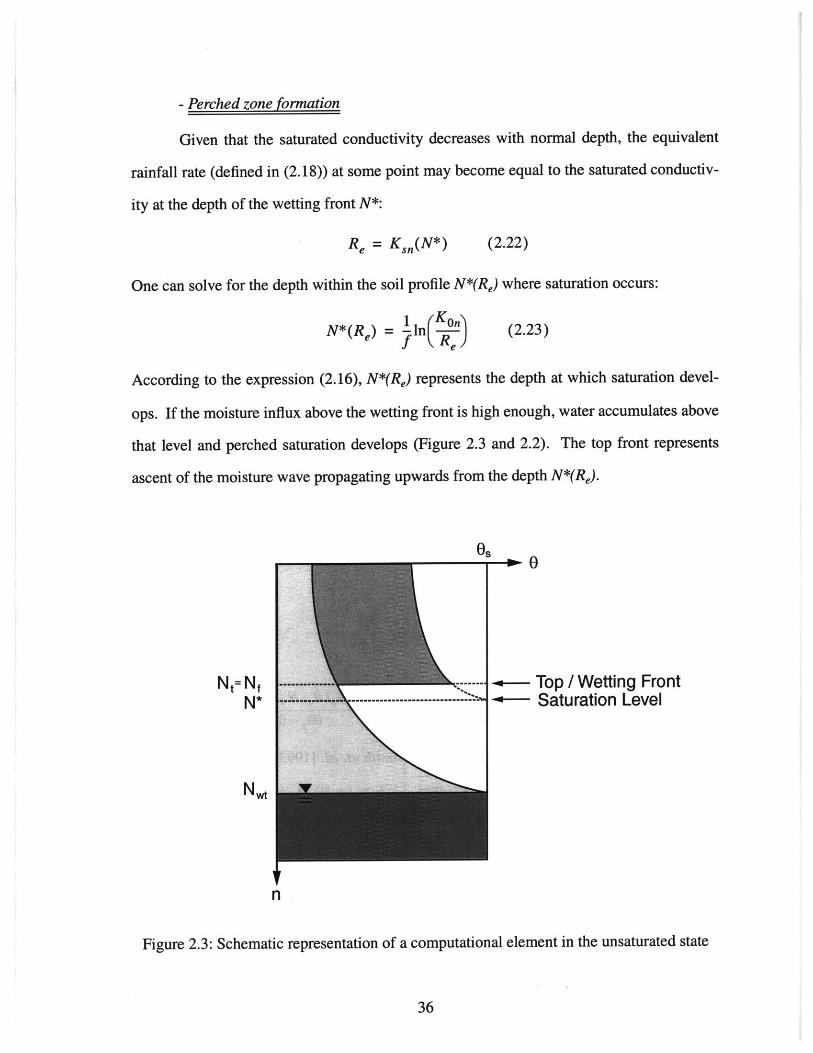
According to the expression (2.16), N*(Re) represents the depth at which saturation devel-
ops. If the moisture influx above the wetting front is high enough, water accumulates above
that level and perched saturation develops (Figure 2.3 and 2.2). The top front represents
ascent of the moisture wave propagating upwards from the depth N*(Re).
Osi Io 0
Nt= NfN*
-- Top / Wetting Front+-- Saturation Level
n
Figure 2.3: Schematic representation of a computational element in the unsaturated state
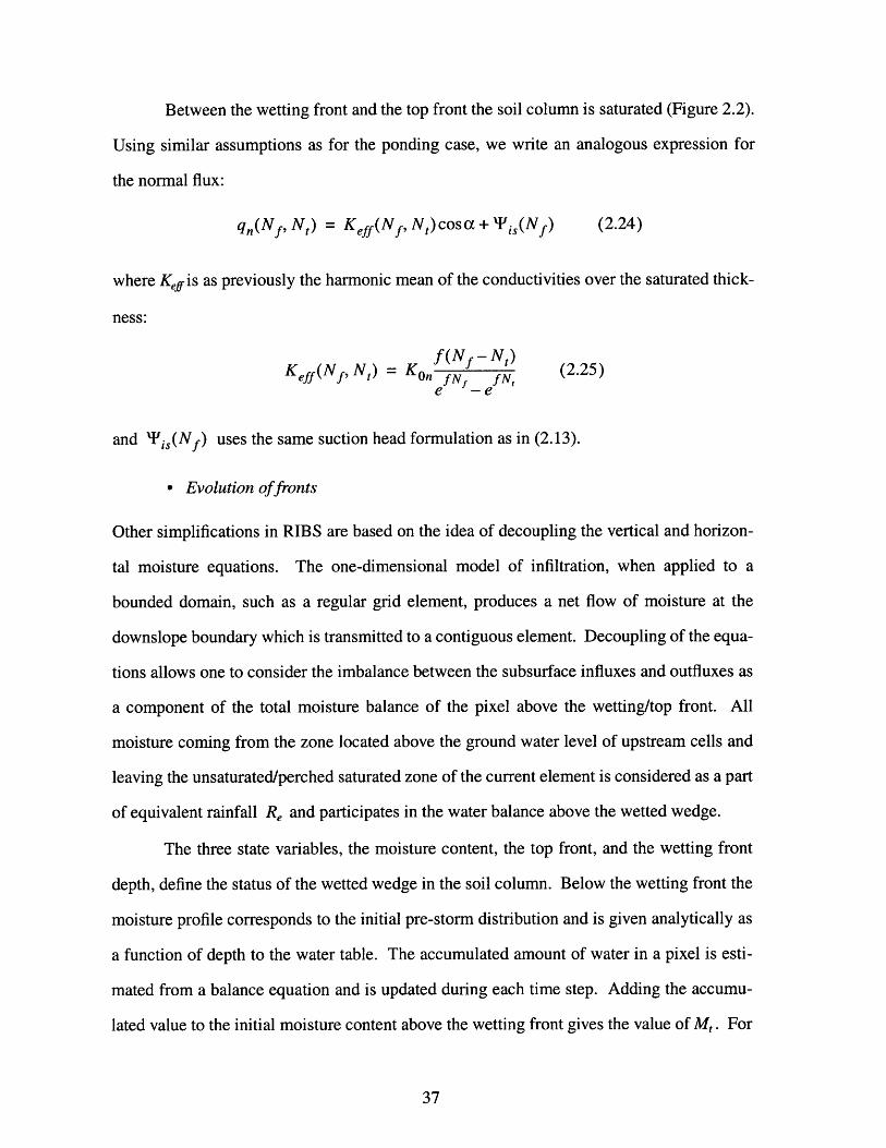
Between the wetting front and the top front the soil column is saturated (Figure 2.2).
Using similar assumptions as for the ponding case, we write an analogous expression for
the normal flux:
qn(Nf, N) = Keff(Nf, N,)cosa +'' i,(Nf) (2.24)
where Kfg is as previously the harmonic mean of the conductivities over the saturated thick-
ness:
Kef (Nf, N,) = K 0 f (Nf N, (2.25)e - e
and Tis (Nf) uses the same suction head formulation as in (2.13).
- Evolution offronts
Other simplifications in RIBS are based on the idea of decoupling the vertical and horizon-
tal moisture equations. The one-dimensional model of infiltration, when applied to a
bounded domain, such as a regular grid element, produces a net flow of moisture at the
downslope boundary which is transmitted to a contiguous element. Decoupling of the equa-
tions allows one to consider the imbalance between the subsurface influxes and outfluxes as
a component of the total moisture balance of the pixel above the wetting/top front. All
moisture coming from the zone located above the ground water level of upstream cells and
leaving the unsaturated/perched saturated zone of the current element is considered as a part
of equivalent rainfall Re and participates in the water balance above the wetted wedge.
The three state variables, the moisture content, the top front, and the wetting front
depth, define the status of the wetted wedge in the soil column. Below the wetting front the
moisture profile corresponds to the initial pre-storm distribution and is given analytically as
a function of depth to the water table. The accumulated amount of water in a pixel is esti-
mated from a balance equation and is updated during each time step. Adding the accumu-
lated value to the initial moisture content above the wetting front gives the value of M,. For

the unsaturated state (Figure 2.4), the wetting front evolution is described by a first-order
differential equation (Cabral et al., 1992; Garrote, 1993) in the form:
dN = qn(Nf)- (2.26)
dt Oe(Re, Nf) - Oi(Nf)
where qn is the redistribution flux value defined in (2.19), 0, (N) and Oe(Re, Nf) are the mois-
ture contents also introduced previously. Equation (2.26) is approximated by the backward
in time finite-difference:
t t-1 t-1
At O(R ,N(-f)-O;(N)- (2.27)
where index "t" defines the time level, and At is the computational time step.
The dynamics of the wetting front for the perched saturated and the surface satu-
rated state (Figure 2.4) are defined as:
dNf qn(Nf, N,)(2.28)
dt OS - 0(Nf)
which is numerically approximated in the same fashion as (2.27).
In the modified RIBS, evolution of the top front in the perched saturated state is dif-
ferent from the formulation used by Garrote [1993]. The original formulation assumes a
discontinuity in the moisture content at the top front: from the land surface the profile fol-
lows the distribution corresponding to N*(Re), the depth at which perched saturation started
developing, and abruptly becomes 0, at the top front (see Garrote, 1993 for details). This
introduces certain difficulties since the moisture profile above the top front can not be easily
treated with arbitrary upper boundary flux conditions, e.g. handling the moisture profile
during the periods of rainfall hiatus or interstorm periods. Instead, it was assumed that the
top front at each time t represents the saturation depth corresponding to some Re . Accord-
ing to (2.23):
N, = N*(R') = In [ (2.29)I .-Re-
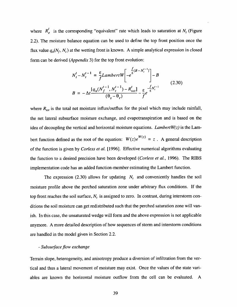
where Rt is the corresponding "equivalent" rate which leads to saturation at Nt (Figure
2.2). The moisture balance equation can be used to define the top front position once the
flux value q,(Nf, Nt) at the wetting front is known. A simple analytical expression in closed
form can be derived (Appendix 3) for the top front evolution:
t t-1 E ~ (B-N -Nt =-LambertW
[ e s] B (2.30)t-1I t-1I t fN'~-1
B -At [n( Nf , N, ) - R tot] 6 e C
where Rtor is the total net moisture influx/outflux for the pixel which may include rainfall,
the net lateral subsurface moisture exchange, and evapotranspiration and is based on the
idea of decoupling the vertical and horizontal moisture equations. LambertW(z) is the Lam-
bert function defined as the root of the equation: W(z)e = z . A general description
of the function is given by Corless et al. [1996]. Effective numerical algorithms evaluating
the function to a desired precision have been developed (Corless et al., 1996). The RIBS
implementation code has an added function-member estimating the Lambert function.
The expression (2.30) allows for updating N, and conveniently handles the soil
moisture profile above the perched saturation zone under arbitrary flux conditions. If the
top front reaches the soil surface, N, is assigned to zero. In contrast, during interstorm con-
ditions the soil moisture can get redistributed such that the perched saturation zone will van-
ish. In this case, the unsaturated wedge will form and the above expression is not applicable
anymore. A more detailed description of how sequences of storm and interstorm conditions
are handled in the model given in Section 2.2.
- Subsurface flow exchange
Terrain slope, heterogeneity, and anisotropy produce a diversion of infiltration from the ver-
tical and thus a lateral movement of moisture may exist. Once the values of the state vari-
ables are known the horizontal moisture outflow from the cell can be evaluated. A

simplified scheme was adopted to account for the moisture transfers between elements.
Gravitational forces are assumed to be predominant in the lateral subsurface water transport
and therefore the kinematic formulation is used to estimate the outflux. The horizontal
component of the gravity-dominated flow can be integrated along wetted depth to obtain the
total discharge from the soil column (Garrote, 1993):
Nfcos a
Q = q (z)dz (2.31)0
where Q is the outflux from the wetted portion of the unsaturated zone (per unit width).
Replacing the integral with the relevant components for the unsaturated and saturated part
of the moisture profile:
N, NfcosaL cosa
Q = f x(z)dz + f q (z)dz (2.32)0 N,
cos a
where the horizontal components of flow for the unsaturated and the saturated portions of
soil are respectively given (Cabral et al., 1992) as:
q, = Recosa -sinc(ar - 1)
= K cs sn cc are-fncosacc f(Nf - N) (2.33)=KOn Cos a - sina are efN e fN, Ie - e-
Substituting (2.33) into the integrals of (2.32) the expression for gravity-driven sub-
surface moisture flux per unit width is obtained (Cabral et al., 1992):
- 2-ar -fN, -fN5 f(Nf - N,)
Q = sina [NtRe(ar-1+ 1Konf(e -e O[ fN e fN '34)
The first square-bracketed term of (2.34) gives the contribution from the unsaturated part of
the wetted profile. If the perched saturation zone exists, lateral discharge is given by all
three terms of (2.34) while N,> 0. In the advanced stages of infiltration N, = 0 and Nf is very
large. Therefore the first term in equation (2.34) is zero, the third approaches zero and the
asecond term has a limit value for large N, given by lim Q = sin aKOn - . The limit value
r >- f
increases with the anisotropy ratio and the surface saturated hydraulic conductivity and
decreases with the decay parameterf.
Expression (2.34) is applied to evaluate outflows for all elements in the basin. The
single preferential direction of the subsurface flow is defined based on the local topography
according to the highest elevation gradient (the "D8" approach referred above). Subsurface
inflow into a certain cell is given by the sum of the outflows from all upstream elements
draining directly into it. In order to account for moisture transfers between elements cor-
rectly, the computations are carried out recursively from the upstream elements down to the
outlet.
As noted by Garrote [1993], several major simplifications are implicit in this
scheme. First, the coupling effect between elements is only indirectly considered. Each cell
is represented by its central node to which the model equations are applied. The coupling
between elements is taken into account in the mass conservation equation, but neglected in
the momentum equation, i.e. the speed at which the fronts move. This is acceptable as long
as the volume of water transferred is only a small fraction of the total moisture content in
the element. The second simplification refers to the assumption about the flow geometry.
The spatial orientation of flows entering a cell is assumed to be parallel to the line of maxi-
mum terrain slope, irrespective of the orientation of the slopes of the upstream pixels and
discontinuities at the pixel boundaries associated with different slopes in adjacent cells.
The assumption is plausible considering the fact that the pixel size is much larger than ele-
vation difference in the contiguous nodes.
- Runoff generation schematic
Both infiltration excess runoff and return flow are represented in RIBS. They are estimated
as the result of evolution of the state variables in the element and reflect the fact of limited
or zero soil infiltration capacity.
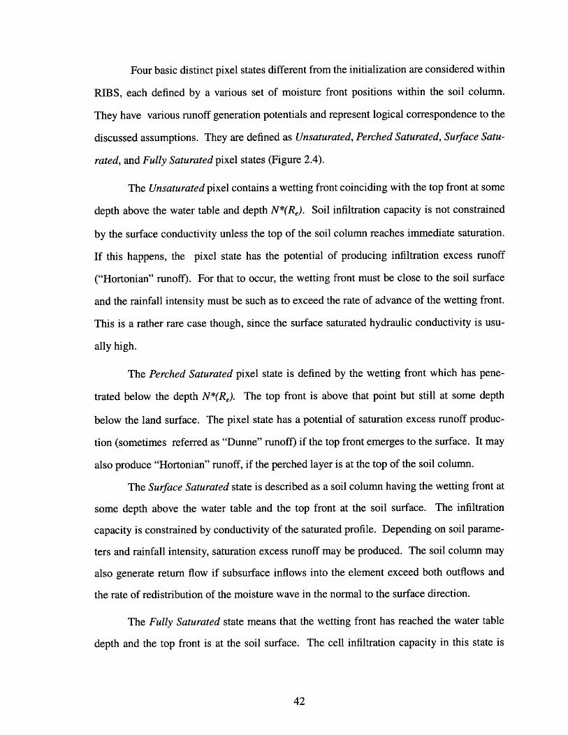
Four basic distinct pixel states different from the initialization are considered within
RIBS, each defined by a various set of moisture front positions within the soil column.
They have various runoff generation potentials and represent logical correspondence to the
discussed assumptions. They are defined as Unsaturated, Perched Saturated, Surface Satu-
rated, and Fully Saturated pixel states (Figure 2.4).
The Unsaturated pixel contains a wetting front coinciding with the top front at some
depth above the water table and depth N*(Re). Soil infiltration capacity is not constrained
by the surface conductivity unless the top of the soil column reaches immediate saturation.
If this happens, the pixel state has the potential of producing infiltration excess runoff
("Hortonian" runoff). For that to occur, the wetting front must be close to the soil surface
and the rainfall intensity must be such as to exceed the rate of advance of the wetting front.
This is a rather rare case though, since the surface saturated hydraulic conductivity is usu-
ally high.
The Perched Saturated pixel state is defined by the wetting front which has pene-
trated below the depth N*(Re). The top front is above that point but still at some depth
below the land surface. The pixel state has a potential of saturation excess runoff produc-
tion (sometimes referred as "Dunne" runoff) if the top front emerges to the surface. It may
also produce "Hortonian" runoff, if the perched layer is at the top of the soil column.
The Surface Saturated state is described as a soil column having the wetting front at
some depth above the water table and the top front at the soil surface. The infiltration
capacity is constrained by conductivity of the saturated profile. Depending on soil parame-
ters and rainfall intensity, saturation excess runoff may be produced. The soil column may
also generate return flow if subsurface inflows into the element exceed both outflows and
the rate of redistribution of the moisture wave in the normal to the surface direction.
The Fully Saturated state means that the wetting front has reached the water table
depth and the top front is at the soil surface. The cell infiltration capacity in this state is

zero. When the wetting front reaches the ground water surface, it is assumed that the water
table is instantaneously transferred to the soil surface. This causes sudden expansion of the
ground water zone of the cell and elimination of its unsaturated portion. If rainfall persists,
the element produces saturation excess runoff. If upstream cells contribute subsurface flow
from the vadose zone to a pixel in this state, return flow is generated. Also, if the net satu-
rated flux in the groundwater system for such an element is positive, groundwater exfiltra-
tion flow is assumed to be produced.
In general, actual infiltration I, rainfall Rn, infiltration capacity f, and runoff Rf
("Hortonian" and "Dunne") can be related as:
I = Rn, Rf = 0 if N,>0, Nf<Nw,
I f,, Rf Rn-fc if N, = 0, Nf<N,,, Rn>fc
1= 0, R = Rn if N, = 0, Nf = Nw,
where Nwt is the water table depth in the element. Return flow is the result of lateral subsur-
face exchange and is produced under similar conditions:
I = fc, Rf = YQs-fc if Nt = 0, Nf<Nwt, IQs>fc
where EQs is the net sum of subsurface lateral inflows and outflows and is positive. The
runoff generation due to the ground water corresponds to the following conditional expres-
sion:
I = 0, Rf = LQsat if N, = 0, Nf = N,
where 2Qsat is the net positive sum of fluxes in the saturated zone. The RIBS ground water
model description is given in Section 2.4.
The total surface flow generated in the element is the sum of all runoff types pro-
duced by the described mechanisms. This runoff is routed to the basin outlet. Re-infiltra-
tion schemes are not presently considered within the RIBS.

Unsaturated (sEMEM~ , I 0
Nf = Nt
Nwt
Perched saturated
Nwt
nSurface saturated 0
MR6 pNt = 0
Fully saturatedNt = 0
Nwt Nf = Nwt
Figure 2.4: Four basic pixel states: Unsaturated, Perched Saturated,Surface Saturated, and Fully Saturated
2.1.3 Surface flow routing scheme
Another aspect in modeling basin response to a storm is routing of generated runoff to the
basin outlet. In Section 2.1.1 a short description of the algorithm used for extracting the
OsE-i*O

flow network from DEMs is given. Runoff produced at any grid point is assumed to follow
that path down to the basin outlet. The detailed geomorphological description of terrain
offered by DEMs provides a good estimate of length of the travel path. The evaluation of
the travel time along that path is a more complicated issue because it involves estimation of
flow velocities which are highly nonlinear due to transient conditions of basin response.
Flow conditions change significantly during a storm. This influences flow velocities and
travel times throughout the basin. A full or approximated form of the Saint-Venant equation
of shallow water flow is usually used to account for bulk transport and flow dispersion in the
real basin. Such a hydraulic routing scheme is physically based and uses information about
watershed flow conditions. However, in order to ease the parameter load and data and com-
puter power requirements, which are the major issue for operation on mid- and large-sized
basins, a simplified parameterization scheme (Garrote, 1993) was implemented allowing to
successfully cope with these problems. The scheme is often referred to as "hydrologic rout-
ing".
The objective of the adopted solution is to differentiate between the two transport
mechanisms that operate in overland and stream flow and to account for some non-lineari-
ties in the basin response. Bulk transport of water is assumed to be the dominant factor in
the basin response and the effect of dispersion is neglected to a first approximation in order
to keep model parameters to a minimum. The distributed instantaneous response function is
assumed to be a Dirac delta function with a delay time equal to the travel time from the
pixel location to the basin outlet. Inclusion of dispersion effects in the formulation is made
in a simplified manner. The method following Garrote [1993] is described below.
The travel path I, for runoff produced on a given hillslope element consists of a hill-
slope fraction lh and a stream fraction 1, (Figure 2.5):
it = lh +is (2.35)
The travel time is defined according to the assumption of uniform velocities for both
overland and stream flows throughout the basin for a given time, although the travel veloci-

ties are allowed to vary as the storm progresses accounting for changing flow conditions in
the streams. If uh(t) is the hillslope velocity and 0,(T) is the stream velocity at time T,
the travel time t, for the typical hillslope element is given by:
t 1 + i+ (2.36)
stream
outlet
Figure 2.5: Schematic representation of a flow path for a hillslope node
The uniform surface velocity approximation allows for a simple computation of the
hydrograph at the basin outlet. Thus at time t the instantaneous response function of the
basin element located at (x, y) would be the Dirac delta function given by:
h,(x, y, t) = -(uh + s (2.37)
An incremental basin response is estimated independently for every time step for the runoff
generated at every pixel:
q,(t) = Rft(x, y)h,(x, y, t)AxAy(x, y) e Catchment
(2.38)
where RfT(x, y) is the runoff rate generated in a cell at location (x, y) at time t and AxAy is
the area of the element. The total basin response at time T is obtained by adding the incre-
mental response since the beginning of the storm:
Q(t) = Y q (t) (2.39)= O
Thus the basin response can be estimated once hillslope and stream velocities are known at
every time step.
Studies and experiments show evidence of non-linear behavior in basin response. It
was assumed that a power law relationship between discharge and flow velocities might
hold (Garrote, 1993) thus reflecting the dependence of travel times on the amount of water
present in the basin. The value selected as an indicator is the discharge at the basin outlet at
the same time. Basin discharge can be thought of as a rough estimate of the conditions in
the drainage network and has the computational advantage of being available at all times.
Thus channel velocities at each time can be obtained using the following expression:
)s(T) = c[Q(T)]r (2.40)
where 1,(T) is the stream velocity at time T, Q(T) is the discharge at the basin outlet at
time T, and c, and r are parameters to be obtained through calibration. It is also considered
that the ratio of stream velocity to hillslope velocity is a constant K, and also has to be esti-
mated through calibration. The travel velocity in hillslopes is thus given by equation:
oh(T) = UQr (2.41)KU
2.2 Transformation to a continuous operation
A rainfall-runoff model intended for use in operational hydrologic forecasting must show
the skill in simulating pre-storm and post-storm conditions in the basin. This requires ade-
quate representation of the ground water system and its runoff production mechansims, as
well as soil moisture redistribution during storm hiatuses and periods of evapotranspiration.
In order to accurately describe interactions between the ground water and unsaturated zone,
a coupling mechanism between them should be developed. Such coupling allows for simu-
lation of ground water recharge as well as accounting for changes in the moisture state of

the unsaturated zone induced by the saturated zone dynamics. All these features are consid-
ered in the modified RIBS version and the following is a description of the basic assump-
tions and techniques implemented within the RIBS framework.
2.2.1 Soil water redistribution and subtraction
The interstorm conditions are modeled using five new RIBS modules dealing with various
pixel transitions that allow for soil moisture redistribution and dynamic adjustments of the
moisture profile during evaporation.
1. The first module calculates the water table drop from the soil surface (n = 0) as a result
of negative mass flux applied at the upper boundary of the computational element (Fig-
ure 2.6). The amount of moisture extracted from the pixel is used to define how deep
the ground water level goes within the time step. An expression is derived for a soil
moisture profile corresponding to a hydrostatic or hydraulic equilibrium assumption (a
more detailed discussion will follow Section 3.2). The Newton iterative scheme is used
to find the solution of a corresponding non-linear equation (Appendix 4). It is efficiently
implemented and leads to convergence within a few iteration steps.
2. The second transition form deals with elements having initial water table located at
some depth below the land surface with negative forcing applied at the upper boundary
of the soil column. Correspondingly, the boundary condition requires subtraction of
water from some portion of the moisture profile which can be done in several ways. The
rationale for the chosen scheme is to keep continuity of the moisture profile in the unsat-
urated zone and conserve mass. The moisture is subtracted from the whole unsaturated
profile which results in drop of the water table for mass conservation (Figure 2.7).
Therefore, the soil moisture profile gets re-initialized. Although the assumption is
strong, it allows for a more convenient treatment of moisture in the unsaturated zone
because of the unique relationship between the water table position and the soil water
distribution given a set of soil parameters.

3. The third module allows for simulation of soil moisture profile transitions during peri-
ods of rainfall hiatus or interstorm periods when a wedge of infiltrated water exists in
the soil (the first three states shown in Figure 2.4). Accounting for the drying cycle pro-
cesses is important (Smith et al., 1993) because of the inherent relationship between soil
moisture and soil infiltration capacity. Ignoring these transitions in the conditions of
intermittent rainfall pulses may lead to a significant underestimation of infiltration vol-
ume. Furthermore, subsurface lateral fluxes may significantly contribute to the descend-
ing limb of hydrograph within the first hours-days after storm termination and hence the
moisture dynamics should be appropriately simulated during this period.
A diagram of the drying cycle is given in Figure 2.8. Immediately after storm ter-
mination, the infiltrated moisture profile redistributes and the surface soil water content
starts decreasing with time. If the duration of the drying period is sufficiently long, the
wetting front may reach the water table and an adjustment of the ground water level will
therefore occur. Depending on the pixel initial state, soil parameters and interstorm
conditions, not all transitions depicted in Figure 2.8 might be present. The moisture
wedge may transit to various states which are briefly discussed below.
Figure 2.6: Illustration of the module estimating water table drop from the soil surface

K'
Figure 2.7: Illustration of the module computing water table drop in a cell having initialground water level at some depth below the soil surface
Figure 2.8: Illustration of the basic drying cycle
- From the Surface Saturated state to the Perched Saturated case (Figure 2.8): if
the normal infiltration flux is higher than the total moisture influx, the moisture pro-
file becomes perched saturated, with the wetting and the top front located at some
depth. This situation may also occur during a storm period, when rainfall intensity
suddenly drops in magnitude.

- From the Perched Saturated profile it may be redistributed to the Unsaturated
profile: the flux at the wetting front depth is high and the recharge rate above the
wetting front is small. After redistribution the top front will coincide with the wet-
ting front (Figure 2.8). This situation may also occur during the storm period.
- In the latest stages of infiltration, the unsaturated wedge will approach the initial
soil moisture profile and, if the wedge soil moisture profile is sufficiently close to the
initial profile, soil moisture excess can be redistributed along it. In order to deter-
mine the need for the procedure, a threshold for the moisture content 0 (Re, Nf) in
the wedge is established. Redistribution of the moisture profile will also occur when
the wetting front reaches the water table. The moisture content in the unsaturated
zone is adjusted to obtain the hydraulic equilibrium profile (Figure 2.8).
The basic governing equations of front and moisture dynamics for all cases
considered above are the same as described in Section 2.1.2. They are applied under
the conditions of zero/negative flux at the upper boundary that results in gradual
wedge de-saturation with time.
4. Two "static" pixels modules are considered in the model. Both refer to the cases when
none of the dynamic variables in the computational element change their values. The
first state refers to the no-flux situation in the element when the moisture profile in the
unsaturated zone stays equal to the initialized state of the pixel. In the second situation,
the water table is located at the soil surface. If no evaporation occurs, or if its rate is less
than the rate of lateral fluxes into the pixel, the water table stays at the surface, influx
excess is accounted as runoff, and all other dynamic variables are set to zero.
5. An artificial soil moisture transition has been added to the model. In fact, it does not
directly deal with the interstorm conditions but is a link from a rainfall event to the
beginning of the interstorm period. It is applied only in the areas with a shallow water
table such as bottoms of convergent hillslopes. During a rainfall period, it is very likely

that the first moisture wave modeled in RIBS as a sharp discontinuity will reach the
water table and therefore the entire soil water profile will be re-adjusted to a new state
with a shallower water table (Figure 2.9). If rain persists, one would expect propagation
of a new wave. However, implementation of this logic leads to a rapidly changing wet-
ting front position in the elements at the hillslope bottom: while in some pixels the sec-
ondary wetting front is starting to develop, in others the first front has not reached the
water table yet. Depending on the initial soil moisture and the subsurface lateral
exchange, the rate of advance of the wetting front will vary for different nodes and
hence at any instantaneous time the cross-section of the hillslope depicting the front
position (as in Rybarczyk, 2000) could resemble numerical instability.
Rainfall
Figure 2.9: Illustration of direct water table re-adjustment
To avoid such an erratic behavior, an assumption is made about how rainfall infil-
trates after the first moisture wave reaches the water table. It is assumed that the mois-
ture added to the initial profile of the vadose zone after the first moisture front reaches
the ground water is sufficient to facilitate propagation of any successive moisture waves
without forming a perched zone. Hence, no runoff production will occur unless the soil
gets completely saturated. The implication in RIBS is that no subsequent fronts are cre-
ated, all water entering the pixel is redistributed along the unsaturated profile and there-
fore the local water table rises. The assumption seems to be reasonable taking into
account that in the majority of cases it is applied to downstream convergent hillslope,
which mostly contribute through the saturation excess runoff and therefore the fronts
position is of secondary concern. It is more important to simulate the rise in the water
table and the saturation stage.
At some point, after the beginning of a no rainfall period, the algorithm must allow
for the creation of a new wetting front. It is assumed that after a given time with no
rainfall the interstorm period begins and any following storm will again generate a wet-
ting front. The no rainfall time that marks the beginning of an interstorm period is
assumed to be climatically dictated and varies for different regions. Commonly, values
are considered to be in the range 1-3 days (Eagleson, 1978). This characteristic time
also marks the time at which redistribution of the moisture excess in the unsaturated
zone has to occur for pixels with an infiltrated moisture wedge. After redistribution of a
wetting front a new water table position is estimated and the resulting soil moisture will
be the initial state for any subsequent storm.
2.2.2 Coupling procedure between fronts of the unsaturated zone and water table.
In order to fully describe the evolution of the unsaturated zone in continuous simulations, a
procedure coupling the dynamics of its variables to the dynamics of the ground water sys-
tem is needed. A simplified algorithm is implemented in RIBS which assumes that when-
ever the wetting front reaches the top of the capillary fringe, a new position of the water
table has to be computed, a statement that has already been made. The new water table
depth will depend on moisture deficit in the unsaturated zone. A Newton iterative scheme
(Appendix 4) is used to estimate it. The procedure allows for dynamic adjustments of mois-
ture distribution in the unsaturated zone and therefore significantly increases model's flexi-

bility. Any changes occurring as a result of ground water dynamics, i.e. changes from
"below", are implemented as part of the ground water model and described in detail in Sec-
tion 2.3.
2.3 Ground water model description
A decoupled 1-D Boussinesq-type equation is applied to a two-dimensional plane of hetero-
geneous anisotropic soil to model the ground water dynamics. The model assumes non-lin-
ear transmissivity which depends on the actual ground water level and bedrock depth.
2.3.1 Formulation of the ground water model
Under Dupuit assumptions, which assume that the equipotential surfaces are vertical with
h = h(x, y) rather than h = h(x, y, z), the Boussinesq's equation for a phreatic aquifer (heter-
ogeneous, anisotropic) with a horizontal impervious base is of the form:
a ah h h yt= A
F[Kxh + K + N(x, y,tt (2.42)
where the terms N and P denote replenishment and pumping (if any), K is the saturated
hydraulic conductivity, S, the aquifer specific yield (for a deep water table can be approxi-
mated by the effective porosity) and h(x, y, t) denotes the elevations of the water table above
an impermeable bottom. A more general form is for the case of a non-horizontal impervi-
ous base rj = Tj (x, y):
a-[Kx(h- ax + a[K,(h- - S, (2.43)
This equation is non-linear in h, however it can be linearized (Bear, 1979) assuming that
variations in the saturated thickness B(x, y, t) = h(x, y, t) - il (x, y) are much smaller than
B(x, y, t) itself. Then, with B(x, y, t) = B(x, y) + b'(x, y, t) and b' B , and
T(x, y) = KB a linearized equation can be obtained:
a +ah , + y - P(x, y, t) = S- T-i +-a [T-y + N(x, y,t)Pxyt) = (2.44)Yx~xx ayL ajY3

where T denotes the transmissivity (L2f/). Assuming N(x, y, t) = P(x, y, t) = 0, homoge-
neous medium (Tx = T), and considering a 1-D case, we can rewrite (2.44):
2
T = S,- (2.45)
where 1 is axis x or y. The specific discharge q of the Darcy's law (1-D case, dimension
L/T) is obtained:
q = -K (2.46)
Hence, the flux Q (L2/T) through an area of unit width is defined as:
-a3h -ahQ = qw = -KB- = -T (2.47)
where o is the cross-sectional unit area of flow.ah.
As implied by the Dupuit approximation, 7 in the right hand of expression (2.47)
is a local slope of the water table, tan(a), where a is the local angle of the ground water
level. It should be multiplied by the width of flow to get equation for cell-to-cell computa-
tion of volumetric flow. Combining (2.47) and (2.45) results in:
ah S3QS =a (2.48)
Applying equations (2.48) and (2.47) in the two-dimensional plain with spatial discretiza-
tion Ax - Ay , each time for one particular "discrete" direction, leads to:
n -Qin QUtj (2.49)eat AxAy AxAy
where ne is the effective porosity modeled as the difference between the saturation moisture
content O, and the residual moisture content Or of the Brooks-Corey parameterization (see
Section 2.1.2), Q1, and Qu, denote inflow and outflow (dimension L3/T) from a grid cell in
j-th direction. A note should be made regarding the effective porosity substituted instead of
the specific yield. For a phreatic aquifer, with non-uniform soil moisture distribution in the
unsaturated zone, the conventional definition of the specific yield is regarded as the volume

of water per unit area of soil, drained from a soil column extending from the water table to
the ground surface, per unit lowering of water table (Bear, 1979). For a ground water level
drop Ah in a phreatic aquifer, the specific yield can be expressed as:
S(Ah, t) =Volume of water drainedS,( h, t) =Ah
n=n, n=n 2
= OsAh + f 0 1(nl, t)dz - f 02(n2, tdz (2.50)Ah[
n=o n=O
where n1 is the water table depth from the ground surface at the beginning, O(n], t) is the
corresponding moisture distribution in the unsaturated zone, n2 = n, + Ah is the water table
depth at the end, and O(n2, t) is the corresponding moisture distribution. The specific yield
can be substituted by the effective porosity ne (assuming there are no moisture infiltration
waves in the vadose zone) if the soil is homogeneous and isotropic and therefore soil mois-
ture curves are identical in shape everywhere. Also both n, and n2 are sufficiently deep
below the ground surface, so that the two soil moisture curves 0(n1 , t) and 0(n 2, t) merge at a
depth close to the soil surface with 0 = Or. The difference between the two integrals
becomes (-Or Ah ) and thus Sy = n,. For shallow ground water this is not true as long as the
moisture distribution curves, corresponding to the two water table positions, are no longer
parallel and the difference between the integrals is not equal to -Or Ah.
From the computational standpoint, treatment of the specific yield according to
equation (2.50) is inconvenient, especially for infiltration events when several moisture
fronts may be present in the vadose zone. An approach of an "implicit" computation of the
specific yield was used instead. Equation (2.47) is used first to compute fluxes in the satu-
rated zone on a cell-to-cell basis. Updated values of the water table are then estimated
based on equation (2.49). A correction of the estimated values of the ground water table is
then made and a corresponding update of all other dynamic variables is conducted. The
adjustment is fully based on the water balance in the element and does not require an

explicit computation of the specific yield. The technique allows one to deal with any mois-
ture state in the unsaturated zone.
The expression for the flux (2.47) can also be re-written taking into account assump-
tions and parameterizations presented in Section 2.1. Normal heterogeneity of soil, param-
eterized as exponential decay of the n-component of the saturated hydraulic conductivity
K0,, (Beven, 1982; Kirkby, 1986), results in a simple equation of depth averaged transmissiv-
ity T with the bottom of bedrock at a known depth 1' = N + B or assumed at infinity:
T = K B = fKpdn = aKOne -dn = arKOn -fN,, -f'
N~ (2.51)
T = KB= lim K 0 pdn = a.One a.K On -fN,
where Nv, is a local normal depth to the ground water table and ar is the ratio between the p-
and the n-components of the saturated hydraulic conductivity. Eventually, the rate of the
saturated subsurface flow to its down-gradient neighbor can be calculated:
(0tj - Tw tanacc......ao (.2Qau = {~wa~~LO (2.52)0 ............... a > 0
where w is the width of flow. Inflows Q,,-s for a particular grid element are defined through
the appropriate ordering structure by assigning outflows from "upstream" cells, i.e. the ele-
ments which have negative hydraulic gradient with respect to the current pixel. A similar
formulation has been used in works by Wigmosta et al. [1994], Wigmosta and Lettenmaier
[1999], Jackson et al. [1996] with differences in interpreting partitioning width of flow w
and in approximation of hydraulic gradient .
2.3.2 Ground water flow partitioning
Grid structures are commonly used in hydrologic modeling to represent different spatial
quantities being analyzed. They are simple to use and convenient but suffer from some

drawbacks. One of the problems is associated with the pixel's flow partitioning. The way
the total outflow is partitioned between adjacent neighbors of a cell depends on the method
used to define flux direction. A significant amount of hydrologic literature in the recent
time has been devoted to this issue (e.g. O'Callaghan and Mark, 1984; Moore and Grayson,
1991; Fairfield and Leymarie, 1991; Quinn et al., 1991; Lea, 1992; Costa-Cabral and
Burges, 1994; Tarboton, 1997). The earliest and the simplest method for specifying flow
directions is to assign flow to only one of the neighbors, either adjacent or diagonal, in the
direction of the steepest descent (O'Callaghan and Mark, 1984). Though this method (des-
ignated in the literature as D8 - eight possible directions) is implemented in the RIBS for
surface flow routing (see Section 2.1), it would be too simplistic to use it for flow partition-
ing in the ground water system which inherently behaves as a medium with a higher degree
of dispersion. Two algorithms are implemented in the current version of RIBS relying on
the works by Quinn et al. [1991], Costa-Cabral and Burges [1994], and Tarboton [1997].
The Multiple-direction method, a version of which is proposed by Quinn et al.
[1991], attempts to solve the major limitation of the D8 algorithm, the one-dimensional rep-
resentation of flow, by weighting flow between all lower neighbor cells in proportion to the
actual slope gradient:
f. S1 L (2.53)
where S is the directional slope, L is an "effective contour length", or a width normal to the
direction of flow j . Values of L are "subjectively chosen by the simple geometrical con-
struct" (Quinn et al., 1991) and assigned to be 0.5 of the pixel size for neighbors in the car-
dinal direction and 0.354 of the pixel size for diagonal neighbors. The procedure addresses
the main problems of the D8 approach with some success. However, examples of using the
method for simple planar, convergent, and divergent topographies (Costa-Cabral and
Burges, 1994; Tarboton, 1997) reveals that spreading of flow from a source pixels results in
unrealistically high dispersion and as a result "the computed (contributing) areas are discon-

tiguous". The method may underestimate fluxes for pixels at particular locations, for
instance saddle points.
Tarboton [1997] introduces a method of defining a single flow direction in the con-
tinuous range between 0 and 2n, the quantity being determined in the direction of the steep-
est negative slope on the eight triangular facets formed in a 3x3 pixel window centered on
the current pixel. This avoids fitting a plane based on elevations of the four diagonal neigh-
bors (as for example in Costa-Cabral and Burges, 1994) and therefore the scheme is robust
and appropriate for any type of cell boundaries. Figure 2.10 illustrates the method. Eight
planar triangular facets are formed between the central node and its contiguous neighbors.
Each of the facets has a downslope vector which when drawn from the center may lie within
or outside the 0 to 450 range. Components of the two vector s, and s2 are given by:
zo - zi
(2.54)
Z1 -- Z2S2~ d2
where z, and di are elevations and distances between pixels as in Figure 2.10.
The facet slope direction ( and magnitude ax are:
Si= atan -
S2) (2.55)
If the vector angle is within the above specified range, it represents the steepest flow direc-
tion on that facet. If the slope vector is outside of the facet angle, the flow direction is
assigned along the steepest edge:
(< 0-+ ( 0 aC = si
d2 d Zo - Z1 (2.56)
((= atan1 - ad1 d1 jd?+d

Column j
Row i
'3
4'
z
8
7
S I
6
I - I, - I -
flow directionz1
|-
I
facet number center node
Figure 2.10: Computation of flow direction on planar triangular facets
The flow direction for the element of interest is taken as the direction of the steepest down
slope vector from all eight facets. A procedure is then used to adjust direction of the vector
to an angle counted counterclockwise from east. It allows for estimation of flow direction
in a continuous range between 0 and 2n . Once the direction and the slope associated with
the current pixel are defined, a boundary segment(s) of the element, through which the flow
is assumed to occur, must be determined. The flow is routed in one or two possible cardinal
directions by specifying a weighted flow width. The weight depends on the quarter where
the direction angle lies. If the flow direction is parallel to the grid orientation, then the exit
width of flow is a single segment of the boundary. If the flow direction is not parallel to the
grid orientation, the exit portion of the boundary consists of two adjacent boundary seg-
ments (see Figure 2.11). The expression for the total flow width is given by Costa-Cabral
and Burges [1994]:
w = |cosC(Ax+Jsin(|Ay
-
12-- ---- - --
(2.57)

Area contributing to I Area contributing to II
Figure 2.11: Flow partitioning across edges of rectangular box
The algorithm is efficient and can deal with any type of possible pixel combination.
This is particularly important because of the dynamic nature of the spatial distribution of the
water table in the basin. A comparison of the implemented schemes of flow partitioning
with analytical solutions of a linearized ground water flow problem is given in Section 4.1.
2.4 Modifications of the ground water module allowing continuousoperation
The original RIBS formulation (Garrote, 1993) did not include a ground water module and
therefore no lateral subsurface saturated fluxes or interaction between the moving fronts in
the unsaturated zone and the water table were allowed. The ground water level, assigned at
the beginning of the simulation as the initial condition, remained unchanged during the run,
except for the cases when a pixel would transition to a fully saturated state (Figure 2.4).
Four new modules dealing with various basic pixel transitions caused by changes in
the ground water level have been added to RIBS. They supplement the model with the
capability of simulating the subsurface saturated flux exchange and make the corresponding
dynamic adjustments of the soil moisture profile in the vadoze zone induced by the subtrac-
tion/addition of water from/to the ground water.

1. The first module considers the case when the total net flux for the current element is
negligible, either in the case when the subsurface influx and outflux are very small or if
they are equal. All of the pixel's dynamic variables are kept unchanged.
2. The next routine describes the pixel transition to the fully saturated state when the total
ground water influx exceeds the gross capacity of the element. Most of the pixel's
dynamic variables are assigned to zero. These are the water table depth and front posi-
tions. The moisture content in the unsaturated zone is also given a value of zero since
there is no unsaturated zone. The influx excess generates the ground water runoff com-
ponent. Any dynamic effects associated with the interaction between the wave of infil-
trated water and the capillary zone are neglected and the water table instantly moves to
the soil surface (an illustration is given in Figure 2.12).
Figure 2.12: Illustration of the module accounting for the transition intothe saturated state caused by the ground water influx
3. The third module deals with the situation when the total saturated outflux in the ground
water system exceeds the total saturated influx and so there is a negative moisture bal-
ance in the grid element. Depending on what the initial state of the pixel is, the module
considers several basic situations.
a.) The water table (the initial depth is denoted as NwtOld) drops in a cell that has the
initialization moisture profile in the unsaturated zone (the top illustration in Figure

2.13). The water table NwtNew, estimated using equation (2.49), has to be modified
because the effective porosity is used instead of the specific yield. As discussed
above, the difference between the two integrals in equation (2.50) corresponding to
the soil moisture curves 0(NwtOld, t) and 0(NwtNew, t) is not generally equal to (-
Or Ah ) and therefore the specific yield Sy can not always be substituted by the effec-
tive porosity n,. Accordingly, the computed water table has to be corrected to satisfy
the moisture balance in the pixel. A moisture deficit dM of the pixel is computed as
the amount of negative moisture balance in the saturated zone summed with the dif-
ference (0NwtOld - MiOld) between the soil's maximum water capacity 0,NwtOld
and initialization moisture content in the unsaturated zone MiOld. The previously
computed value of the water table depth NwtNew is adjusted by finding a root of the
corresponding analytic equation using the Newton iteration procedure (the descrip-
tion is given in Appendix 4). The previously computed water table depth is used as
an initial guess.
b.) The water table drops in an element that has a wetted wedge in the unsaturated zone
(the middle illustration of Figure 2.13). The value of the ground water level, com-
puted using equation (2.49), has to be modified as in the above case to satisfy the
moisture balance in the element. This is done in the same way as described above:
an adjusted value of the water table depth NwtNew is estimated based on the mois-
ture deficit in the unsaturated zone excluding moisture contained in the wedge of
infiltrated water. However, the updated value of the water table depth affects the
wetted wedge because the initial state of the vadose zone has been wetter (as the
water table goes down, the initialization moisture profile becomes drier, Figure
2.13). The solution adopted is to re-define the equivalent recharge rate Re (referred
as RuNew in Figure 2.13) based on the moisture amount contained above the wetting
front. This moisture amount Mu is equal to the total amount of infiltrated water plus
the initialization moisture contained above the wetting front. The latter quantity is

reduced relative to the initial state, before the drop in the water table level (this
"lost" amount is illustrated as a dark shaded area between the dashed and solid lines
showing the initial and final initialization soil moisture curves, Figure 2.13).
Knowledge of M, allows for computation of RuNew using equation (2.18). If the
water table drop causes the wedge to become too dry, i.e. the moisture content
o (Re, Nf) (see Section 2.2.1) becomes less than a threshold value, the moisture
excess may be redistributed along the initialization profile.
c.) The water table drops in a cell which is either in the perched or surface saturated
state (the bottom illustration of Figure 2.13). Similar to the above cases, an update
of the water table position is made to account for using the effective porosity instead
of the specific yield. The water table drop again leads to a drier initialization mois-
ture profile and therefore this has an impact on the moisture amount contained above
the wetting front (the dark shaded area between the dashed and solid lines showing
the initial and final initialization soil moisture curves illustrates the moisture amount
that has to be taken into account). The assumption made in the model is to subtract
the amount out of balance from below the wetting front thus obtaining its new value
NfNew. This operation satisfies the moisture balance in the pixel and minimizes pos-
sible feedbacks related to the infiltration capacity of the cell. The new front position
is obtained using a mass-conserving iteration procedure. A detailed description is
given in Appendix 5.
4. The last of the added modules handles pixel transitions when the total saturated influx in
the ground water system exceeds the total outflux and so there is a positive moisture bal-
ance. Depending on possible initial states and the magnitude of the difference between
the fluxes, several basic situations are considered.
a.) The water table rises in an element which does not have the wave of infiltrated water
(the top illustration in Figure 2.14). As above in 3-a, correction of the computed
water table NwtNew is made to satisfy the mass balance.
b.) The water table rises in a pixel that has a wetted wedge in the unsaturated zone.
Depending on the magnitude of the positive moisture balance in the saturated zone
and the initial front position, NfOld, the new water table, NwtNew, may go up high
enough to reach the wetting front from below. If it does not reach it (the middle
illustration in Figure 2.14), then modeling of this situation is similar to the consid-
ered above case 3-b. The only difference is that after correcting the water table
depth the initialization moisture profile becomes wetter. The equivalent recharge
rate RuNew is similarly updated based on the moisture amount contained above the
wetting front (see discussion in 3-b).
If after the water table adjustment, the ground water level does reach the wetting
front from below (the top illustration in Figure 2.15), the adopted solution assumes
that any dynamic effects associated with the wetting front - capillary zone interac-
tion are neglected and a new "initial" profile is computed for the unsaturated zone.
The total moisture deficit dM in the unsaturated zone is computed as the amount of
positive moisture balance in the saturated zone summed with the infiltrated amount
of water and the difference (0, NwtOld - MiOld). Appendix 4 describes the proce-
dure of finding the water table depth NwtNew' given a value of dM.
c.) The water table rises in a pixel that is in the perched saturated, or surface saturated
state (the bottom plots in Figure 2.14, 2.15). As in the above discussion, the subse-
quent adjustments depend on whether the water table reaches the wetting front from
below. If it does not, the case is similar to 3-c with the difference being that a rising
water table leads to a wetter initialization moisture profile. The assumption made in
the model is to add the necessary water amount below the wetting front to obtain a
new value NJNew. The new front position is obtained using a mass-conserving iter-
ation procedure. A more detailed description is given in Appendix 5.
If after the water table adjustment, the ground water level does reach the wet-
ting front from below (the bottom illustration in Figure 2.15), the adopted solution

assumes that any dynamic effects associated with the wetting front - capillary zone
interaction are neglected and the unsaturated zone of the element instantly becomes
a new initial state. The total moisture deficit dM in the unsaturated zone is com-
puted as the amount of positive moisture balance in the saturated zone summed with
the infiltrated amount of water and the difference (OSNwtOld - MiOld). Appendix 4
describes the procedure of finding the water table depth NwtNew' given a value of
dM.

NwtOld 4
4- NwtOld 4
NfOld 4
4- NwtOld 4
4- NwtNew
4- NwtNew
4- NfNew
4- NwtNew
Figure 2.13: Illustration of the module accounting for the water table drop in theunsaturated zone - ground water coupling scheme
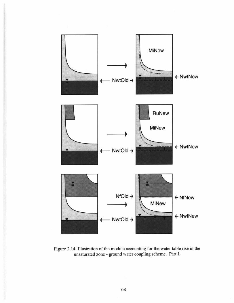
4- NwtNew4- NwtOld 4
-4
4- NwtNew4 NwtOld 4
NfOld 4-4
4- NfNew
4- NwtNew4- NwtOld 4
Figure 2.14: Illustration of the module accounting for the water table rise in theunsaturated zone - ground water coupling scheme. Part I.
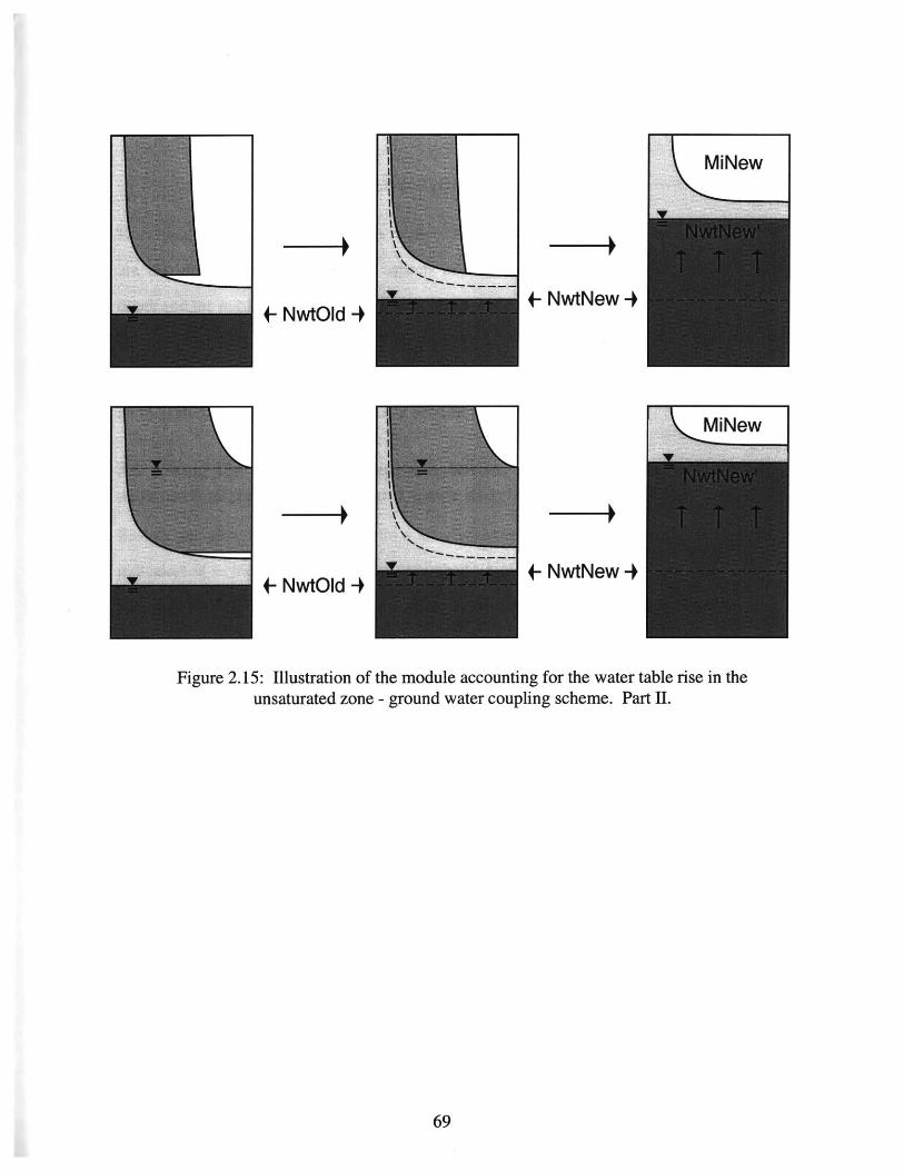
4- NwtOld 4
- NwtOld 4
- NwtNew 4
4 NwtNew 4
Figure 2.15: Illustration of the module accounting for the water table rise in theunsaturated zone - ground water coupling scheme. Part II.

70
CHAPTER III
Initialization Schemes
Knowledge of the initial conditions is required for modeling rainfall-runoff response. There
are two distinct but interconnected aspects of basin initialization: the initial water table
depth and the initial moisture profile in the vadose zone. The chosen approach assumes that
depth to the water table controls both the magnitude of the initial soil moisture deficit and
the type of the soil water profile. It emphasizes the distribution of the ground water level as
an indicator of initial catchment wetness conditions.
3.1 Fixing the water table depth: overview of strategies and a modifiedapproach of steady-state ground water distribution
Basin streamflow at the outlet prior to a simulated event can be considered as one of the
indicators of wetness conditions in the watershed. A plausible way of simulating the initial
water table distribution could be to let the basin drain until the outlet discharge corresponds
to the observed pre-event baseflow. At this time, the water table topography can be used as
the "best" initialization guess. However, significantly different ground water level distribu-
tions may correspond to the same streamflow value. These different solutions correspond to
various parameter sets that define the rate at which the ground water system releases water
to generate baseflow. For example, specifying low hydraulic conductivity for the phreatic
aquifer will result in a shallower water table depth distribution than in the case if high
hydraulic conductivity values were used. Other difficulties are associated with arbitrarily
assigning an initial distribution of ground water depth. Fixing the water table depth at zero
or some constant depth for the whole basin introduces a lot of noise in the ground water
topography. It takes significant computational effort to reach steady flow conditions in the
ground water system and therefore the overall efficiency of this method is unsatisfactory.

- ---- U---- - -
Another proposed strategy (Entekhabi, 1999) is to drive the model with low inten-
sity rainfall for very long time starting with some guess of water table distribution (for
instance, very deep). Expression (2.49) can be used as a basis for modeling the ground
water dynamics. Different water table distributions can be obtained corresponding to differ-
ent baseflow values. They will still be dependent on the soil hydraulic parameter values
used in the ground water model and lead to the same problem discussed above. Moreover,
the computational efficiency would be a serious issue for mid- to large-sized catchments.
The conclusion one can make is that only using baseflow as a guide to ground water initial-
ization leads to non-unique solutions. Additional information and assumptions regarding
the ground water system have to be made.
An alternative is to use an equilibrium hydrology approach (Berger K.P., 2000; Sal-
vucci and Entekhabi, 1994) which couples the unsaturated and the saturated zones through
the assumption of long-term stationarity of the mean moisture state. The dynamic equilib-
rium is maintained by an assumed net recharge flux which either drains to or discharges
from the saturated zone. The time-averaged soil moisture profile which transmits the long-
term mean recharge can be computed based on the analysis of equilibrium values of hydro-
logic fluxes under soil- and climate controlled boundary conditions. This steady moisture
profile is equal to the temporal mean moisture profile in linear soils and an adequate approx-
imation of the mean in non-linear soils (Salvucci and Entekhabi, 1994). An iterative proce-
dure coupling the saturated and the unsaturated zones should then be used to obtain a
spatial water table distribution satisfying the condition of equilibrium recharge rate in the
vadose zone. A deficiency of the method is that determination of equilibrium recharge rate
cannot be obtained without preliminary off-line simulation of hydrologic fluxes at the catch-
ment scale. This is a time and effort consuming procedure. Another major problem is that
the approach lacks explicit use of "real-time" information about the basin wetness. The
relevant methodology should employ any measurable watershed hydrogeologic characteris-
tics as well as features of the recession flow and any other pre-storm conditions.

An approach presented by Sivapalan et al. [1987] is used for the model initializa-
tion. The approach is based on the assumption of quasi steady state conditions in the
ground water system. It assumes that the recession streamflow discharge prior to a storm
Q(t=O) results from a steady rate of recharge to the water table. A spatially uniform
recharge rate is assumed and it is defined as Q(t=O)/A , where A is the total area of the
basin. The next assumption made is that each point in the basin contributes to the steady
state streamflow Q(t=O) proportionally to its surface contributing area. For a particular
location this gives;
=aQ(t=O) (3.1)A
where q, is the saturated flow beneath the water table, and a, is the surface contributing area
draining through a pixel per unit contour length. It is further assumed that the water table is
parallel to the soil surface. Therefore the principal direction for subsurface flow can be
approximated with the direction of the highest topography gradient. Combining the second
form of the transmissivity formulation (2.51), the expression for the saturated subsurface
flow rate (2.52), and equation (3.1) results in:
1 acfQ(t=) -N =--lnLA 1] (3.2)"'f [AK~narWtan%_
where Ng, is the local depth to water table at time t = 0; Kon is the surface saturated conduc-
tivity;f is the decay parameter of the saturated conductivity; ar is the anisotropy ratio, W is
"width" of the saturated flow between cells, and $ is the terrain surface slope. The expres-
sion can be integrated (as in Sivapalan et al., 1987; Larsen et al., 1994) to get the mean
depth to the ground water in the basin:
N = fN,,d A (3.3)
A
N = {n - In an dA +fN (,ln(Toar) - ln(Toar)dA}A A
Knwhere To = is a transmissivity coefficient of the saturated profile. The above
equation can be re-written to give the local depth to the water table in terms of deviations
from the mean value:
N = F {- In( ' -c -(ln(Toar)-Y) (3.4)
X = n dA
A
y = fQln(Toar)dAA
According to (3.4), the local depth to the water table is the deviation from the mean
water table depth value expressed as a scaled quantity of the deviation in the local topo-
graphic index away from its areal integral value X, and the deviation in the local transmis-
sivity away from the basin hydrogeologic constant y. Computed values of No, less than
the thickness of the capillary fringe zone (defined in Section 3.2 as equal to the absolute
value of the air entry bubbling pressure I yv 1) depict saturated cells with water table located
at the soil surface.
As it can be seen, formulation (3.4) requires a minimum of the parameters: ar , KOn
f, and N . Sivapalan et al. [1987] and Troch et al. [1993] discuss how to estimate the mean
depth to the water table and soil hydraulic properties based on the recession flow analysis.
All other information is estimated from the catchment DEM.
Because the definition of surface contributing area within the framework of RIBS is
defined based on the D8 method (see Section 2.3.2 for details), it directly follows from (3.2)
and (3.4) that a sudden increase in the upslope contributing area results in a local jump of
the estimated water table value. For example doubling the contributing area ac leads to a
change in the water table depth by a factor of ln(2). Another factor causing abrupt changes
in the position of the water table is a sharp decrease/increase of the surface slope 6. Zero

slope at some locations also leads to problems in the objective evaluation of (3.4) and dis-
tortions in the calculation of the catchment topographic index X.
In order to resolve these difficulties, the water table depth is corrected and
smoothed. Two procedures are applied. In the first procedure it is assumed that the topo-
graphic index (ln(a/Si)) can be described by a normal distribution (lognormal distribution of
a/S1 ). The topographic index of the hillslope pixels, defined as the ones that have contribut-
ing area less then a threshold value (see Section 2.1), is checked and forced to be within ±2
standard deviations of the 95% confidence interval. The second procedure is a simple
smoothing algorithm. A moving average is computed in the window of 5x5 contiguous pix-
els. The averaging is used 2-3 times until a sufficiently smooth distribution of the water
table topography is achieved. An example of the water table topography before and after
applying the filtering algorithms is given in Figure 3.1. The procedure results in the desired
dendritic shape of the water table topography (Figure 3.2).
An independent software routine has been developed to implement the described
initialization procedure. It can be used to generate an ensemble of the ground water distri-
bution states corresponding to various soil hydraulic properties and the mean water table
depths. As long as the water table depth dictates the soil moisture distribution in the unsat-
urated zone (discussed further in Section 3.2), the ensemble of the ground water level distri-
butions corresponds to different wetness conditions. A lower value of the mean depth to the
water table in the basin would correspond to a wetter initial state and a higher value would
correspond to a drier state. Based on the information about the actual antecedent conditions
prior to a simulated storm event, more likely sets can be chosen to serve as a basis for subse-
quent calibration analysis.
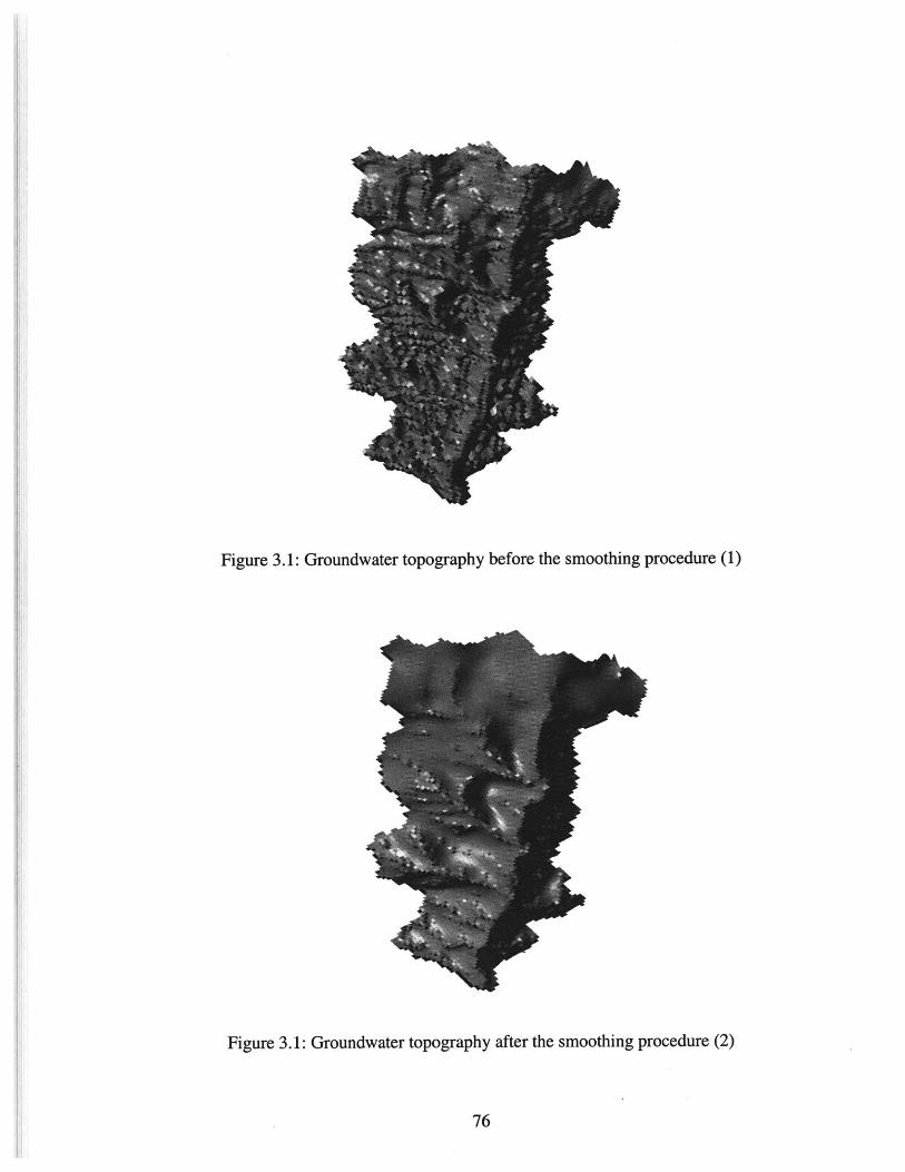
Figure 3.1: Groundwater topography before the smoothing procedure (1)
Figure 3.1: Groundwater topography after the smoothing procedure (2)

18000
16000
14000
12000
1000
Figure 3.2: Estimated depth to the water table. Peacheater Creek, OK
3.2 An overview of soil moisture initialization schemes. Hydrostatic equi-librium moisture profile.
A common problem in rainfall-runoff modeling is specifying the initial moisture state of the
catchment. It is handled differently in various models depending on the model type and
basic assumptions of the hydrologic framework. Many models need to specify soil mois-
ture distributed over a certain spatial domain in an explicit fashion. This can be done using
remotely sensed or in-situ data of the near-surface soil water content and making some
assumptions about how the profile is distributed from the land surface down to the water
table. Similarly, knowledge of the water table depth can be used to initialize the distribution
of moisture in the unsaturated zone. The soil moisture profile can also be constructed
numerically based on the assumed recharge rate to the groundwater. A discussion of these
methods follows.

The original RIBS initializes the soil moisture profile (Cabral et al., 1992; Garrote,
1993) using a non-linear dependence of the initial recharge rate on the depth to the water
table. It is derived from the kinematic approximation of infiltration model which assumes
that gravity alone defines the infiltration flux within the unsaturated zone. A steady-state
moisture profile, that maintains an unsaturated hydraulic conductivity equal to the rainfall
rate, can be derived under these assumptions (see Cabral et al., 1992 for details). The satu-
ration depth in this profile defines the ground water level as long as the capillary fringe zone
is neglected (Figure 2.2). Conversely, knowledge of the water table depth allows one to
uniquely identify the recharge rate as well as the soil moisture distribution within the unsat-
urated zone (equation (2.16)). The expression below defines the initial recharge rate, R;, as
depending on the depth to the water table, N, , and decay rate,f, of the saturated conductiv-
ity Ko0 :
R; = KOne fN'' (3.5)
This approach is computationally convenient but leads to some undesired effects. The
major problem is in soils where the value of f approaches zero. In this case, the recharge
rate tends to be equal to the surface saturated conductivity Kon and, correspondingly, the
moisture profile approaches complete saturation O(R , n) ~ Os
- i fn~(0 Re --- 0
lim O(Ri, n) = lim (sf -+*0 f -+ 0 (Kof(n - N,).
= lim e E (OS -O + Or OS (3.6)f -OL0_
(this expression is obtained by combining equations (2.16) and (3.5)). This leads to less
flexibility in parameter calibration because minor changes in the decay parameterf result in
rather significant changes in the initial moisture state of the basin. Furthermore, this prohib-
its using f values lower than a certain threshold, which otherwise may result in the initial-
ization close to complete saturation. This is an unacceptable drawback. The desired soil

moisture initialization parameterization should be less dependent on the conductivity decay
parameterf.
One of the most commonly used approaches in initializing the moisture profile in the
unsaturated zone is to consider a uniform distribution of soil water throughout the whole
thickness of the vadose zone (e.g. Senarath et al., 2000; Smith et al., 1993; Mein and Lar-
son, 1973; etc.). This parameterization decouples the distribution of moisture in the unsat-
urated zone from the water table position. It is thus highly flexible and allows one to both
easily modify values of moisture content in the desirable range and conveniently incorpo-
rate remotely sensed or in-situ data in the hydrologic analysis. Most of the off-line infiltra-
tion models use this approach to initialize an infinitely deep soil column with some constant
moisture value throughout the depth and consequently apply meteorologic conditions of
storms and interstorm periods as the upper boundary condition (e.g. Smith et al., 1993;
Charbeneau and Asgian, 1991; Corradini et al., 2000). As water infiltrates, the soil mois-
ture distribution is dynamically updated in the form of computed profiles. No interaction of
moving fronts with the groundwater level is usually considered.
Decoupling the soil water distribution in the unsaturated zone from the controlling
effect of the ground water level ignores the obvious physical relationship. It implies that the
spatial distributions of both variables are independently specified which creates an addi-
tional initialization problem. Within the framework of the RIBS model, such a parameter-
ization would cause a problem associated with the dynamic soil water profile adjustments.
The infiltration model allows only one wave of infiltrated water to be present at any instant
of time in the unsaturated zone (discussion is given in Section 2.2). All incoming moisture
is considered as a part of the water balance of this moisture wedge. This condition must be
relaxed at some point, either at the time when the wetting front reaches the water table or
when the moisture excess has to be redistributed in the unsaturated zone (see Section 2.2 for
details). In either case, difficulties would arise in initializing the soil column afterwards.
The moisture profile can not be updated as in the case with schemes allowing multiple

fronts for which any successive moisture state is defined based on the previous infiltration
history.
Another possible way to initialize the moisture profile in the absence of measure-
ments is to use the approach discussed by Salvucci and Entekhabi [1994]. The essence of
the approximation is a reconstruction of the moisture profile based on knowledge of both
the steady flow rate in the vadose zone (recharge or capillary rise) and the depth to the water
table. Salvucci and Entekhabi [1994] designed an experiment in which the unsaturated
zone system was subject to climate forcing simulated by a stochastic model, essentially the
one used in Eagleson's [1978] equilibrium water balance model. Salvucci and Entekhabi
[1994] discuss in detail the "equivalent steady profile", or the unsaturated zone moisture
profile that transmits the mean flow of moisture exchange with the saturated zone. They
argue that the profile approximates well the mean initial conditions, i.e. the mean of all the
profiles at the beginning and the end of each storm event, particularly in soils with a deeper
water table. Salvucci and Entekhabi [1994] argued that the equivalent steady profile there-
fore should form a better condition to initialize infiltration and exfiltration capacities. The
long-term mean column flow of moisture exchange between the vadose zone and the satu-
rated zone can be computed based on the analysis of hydrologic fluxes under soil- and cli-
mate controlled boundary conditions. It has been shown that under certain assumptions
regarding soil hydraulic parameterizations for homogeneous and heterogeneous soils, this
soil moisture profile can be found either exactly (Gardner, 1958), approximately (Salvucci,
1993), or numerically (Warrick and Yeh, 1990).
However, the determination of the time average column flow cannot be obtained
without preliminary off-line simulation of hydrologic fluxes at the catchment scale. Useful
for general hydrologic analysis, it represents a time- and effort-consuming procedure for
continuous modeling. Purely numerical treatment of the moisture profile results in poorer
computational efficiency of the model. It is also inconvenient for treatment within the RIBS
of infiltration model. The problem mentioned above, i.e. how to re-initialize the soil mois-

ture profile when the wetting front reaches the water table or when the moisture excess has
to be redistributed in the unsaturated zone, would still occur. There is no apriori suitable
way to determine the soil column recharge rate for these cases.
Another possible strategy is to assume that the depth to the water table significantly
controls wetness conditions in the basin. With this assumption, the ground water level dis-
tribution defines the initial wetness state of the watershed and therefore the soil's initial
infiltration capacity. The implemented approach assumes hydrostatic equilibrium for the
vertical distribution of pressure head which corresponds to zero initial flux in the unsatur-
ated zone: - 1. This assumption appears to be plausible for soils with higher hydraulican
conductivities for which the equilibration time scale is of the order of hours - days. The
approach is simple and allows one to obtain a closed-form analytical relationship between
the depth to the water table and the distribution of soil moisture in the unsaturated zone.
Salvucci and Entekhabi [1994] pointed out that for shallow water table conditions the
hydrostatic profile is an accurate estimate of the temporal mean of pre-storm soil moisture
profiles and therefore is a reasonable estimate of initial conditions. It was successfully used
in a number of rainfall-runoff models (Troch, et al. [1993b], Sivapalan et al. [1987], Coles
et al. [1997], Famiglietti and Wood [1991]).
One of the disadvantages of this type of soil moisture profile initialization for rain-
fall-runoff modeling is that the surface soil moisture varies little for most of the ranges of
water table depths (Figure 3.3) being very close to the residual moisture content Or. There-
fore, the parameterization is not very flexible in terms of variation of the initial conditions in
space (Figure 3.4).
Salvucci and Entekhabi [1994] argued that for deep water table depths, the hydro-
static distribution underestimates the initial surface soil moisture available for exfiltration
and therefore departures of evaporation from potential may occur more often. Another
parameterization caveat is the contradiction between the assumed uniform recharge scaled
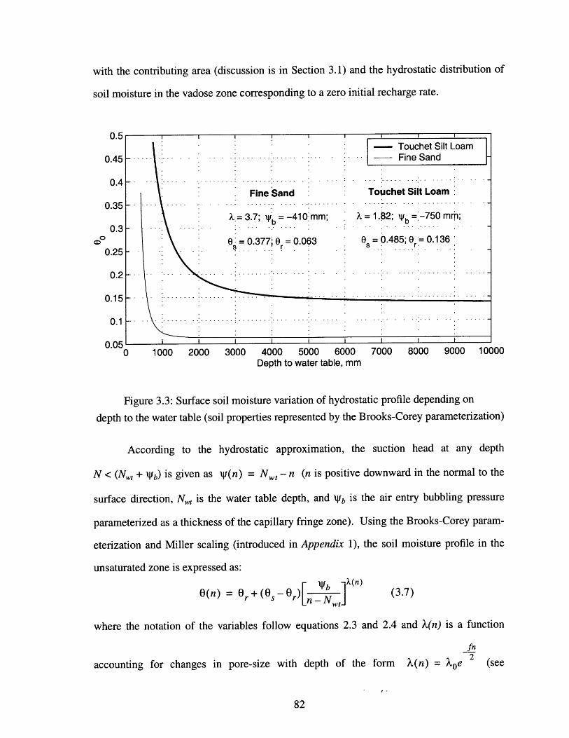
S-.- . 1L~P
with the contributing area (discussion is in Section 3.1) and the hydrostatic distribution of
soil moisture in the vadose zone corresponding to a zero initial recharge rate.
- Touchet Silt LoamFine Sand
Fine Sand
=3.7; =-410 mm;
0 = 0.377 0 = 0.063:
........ .... .... ..-
Touchet Siit Loam
X = 1.82; qb =*-750 mm;
Os = 0.485; Or = 0.136
I I I I I I I
0 1000 2000 3000 4000 5000Depth to water table, mm
6000 7000 8000 9000 10000
Figure 3.3: Surface soil moisture variation of hydrostatic profile depending on
depth to the water table (soil properties represented by the Brooks-Corey parameterization)
According to the hydrostatic approximation, the suction head at any depth
N < (N,, + N) is given as W(n) = N,, - n (n is positive downward in the normal to the
surface direction, N, is the water table depth, and Wb is the air entry bubbling pressure
parameterized as a thickness of the capillary fringe zone). Using the Brooks-Corey param-
eterization and Miller scaling (introduced in Appendix 1), the soil moisture profile in the
unsaturated zone is expressed as:
0(n) = 0r+(0s 0r) [] (3.7)
where the notation of the variables follow equations 2.3 and 2.4 and X(n) is a function
fn
X(n) = Xe 2accounting for changes in pore-size with depth of the form
0.5
0.45
0.4
0.35 F
0.3
0.25
0.1 H
0.05
(see
I/ -
i i i i I I I I
0.2 -
0.15-

Appendix 1). Typical soil water profiles estimated using equation 3.7 for different f values
are given in Figure 3.5. As it can be seen, the higher the decay parameter f, the larger the
departure of the hydrostatic profile from the profile for uniform soil (f= 0). In a medium
where the effective pore size sharply decreases with depth, the larger amount of moisture is
assumed to be bound to the soil particles.
IIle
Basin boundary0o moisture content
0.136-0.18) 0.18 - 0.224
0.224 - 0.267- 0.267 - 0.311
- Z0.311 - 0.3540.354-0.3980.398 - 0.441
S--0.441 - 0.485No Data
1 0 1 2 Kilometers
Figure 3.4: Surface soil moisture corresponding to the hydrostatic assumption of pressure
distribution in (Touchet silt loam, Brooks-Corey parameterization)

0 0
X 3.7 b -410 mm
500 - 0.377 - = 0.063 500 f 0.-0 -mm
1000 -- -- - - -.-.- . -.-.-.- - 1000 --.-.-.-.-.- . -. =O . 1m m
E EE f =0.003 rnm- E
-C 1500 -c 1500
CD) ca-.(1= 0.001 (-
f =0.0
2000 .... - - -- - - - - 2000 ... .-. -.-.
X 1.8 2 b -750. mm
2500---- -. - 2500- --
f =0.0 mm 0 = 0.485 0 = 0.136S r
3000 3000 t0 0.1 0.2 0.3 0.4 0 0.1 0.2 0.3 0.4
0 0
Figure 3.5: Soil moisture distribution corresponding to the hydrostatic assumption inBrooks-Corey soils
The expression 3.7 is consistent with the assumptions made in Appendix 1 and can
be used where soil hydraulic properties are available at a fine spatial resolution. However,
the usual situation is that detailed soil and bedrock coverages for a basin are unavailable.
The catchment is often represented with a few soil types extending over large areas. There-
fore, from a practical point of view, it is very rare that a sharp decay of the saturated con-
ductivity can be assumed. If a soil's f value is rather high, then the lateral moisture
movement in the saturated zone is very limited even for shallow water table conditions.
Fine Sand Touchet Silt Loam
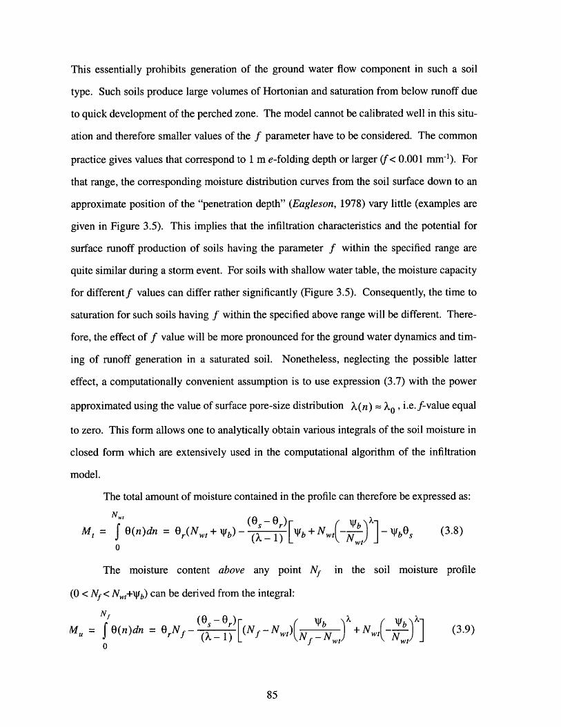
This essentially prohibits generation of the ground water flow component in such a soil
type. Such soils produce large volumes of Hortonian and saturation from below runoff due
to quick development of the perched zone. The model cannot be calibrated well in this situ-
ation and therefore smaller values of the f parameter have to be considered. The common
practice gives values that correspond to 1 m e-folding depth or larger (f< 0.001 mm-1). For
that range, the corresponding moisture distribution curves from the soil surface down to an
approximate position of the "penetration depth" (Eagleson, 1978) vary little (examples are
given in Figure 3.5). This implies that the infiltration characteristics and the potential for
surface runoff production of soils having the parameter f within the specified range are
quite similar during a storm event. For soils with shallow water table, the moisture capacity
for differentf values can differ rather significantly (Figure 3.5). Consequently, the time to
saturation for such soils having f within the specified above range will be different. There-
fore, the effect of f value will be more pronounced for the ground water dynamics and tim-
ing of runoff generation in a saturated soil. Nonetheless, neglecting the possible latter
effect, a computationally convenient assumption is to use expression (3.7) with the power
approximated using the value of surface pore-size distribution X(n) ~ X , i.e.f-value equal
to zero. This form allows one to analytically obtain various integrals of the soil moisture in
closed form which are extensively used in the computational algorithm of the infiltration
model.
The total amount of moisture contained in the profile can therefore be expressed as:
"" (0s -Gr Od[ +Nt b W 38t = 0(n)dn = 0r(Nw,+ Vb) (X_) [b N (3.8)
0
The moisture content above any point Nf in the soil moisture profile
(0 < N< N,+Ib) can be derived from the integral:
u= 0(n)dn = OrNf - (N;-N N bN +N - (3.9)0

The moisture content at any point lower than Nf in the soil moisture profile
(0 < Nf < Nt+lb) has a form:
N,,
MI = 0(n)dn =Nf (3.10)
= r(Nwt + 19 - Nf) - ( O -1 [b+(N,-Nf) NN) j bos

CHAPTER IV
Model Performance: Synthetic Off-line Tests
4.1 Test case: ponded infiltration into a semi-infinite soil column
In order to test the assumptions of Section 2.1 for the modified Green-Ampt model and to
study the performance of the infiltration model at the subgrid scale, several different scenar-
ios of ponded infiltration are simulated. For each of the cases, a soil hydraulic parameter
involved in the parameterization of the Darcian flux equation defined by (2.14) is varied. A
semi-infinite soil column is considered in the test, i.e the soil having infinite lateral extent
and bounded by the water table from below. No lateral moisture movement is allowed. The
infiltration process is induced by rainfall applied at the upper boundary. It is further
assumed that the rainfall rate is equal to the infiltration capacity of the soil at any instanta-
neous time and therefore the ponding depth, ho, is zero. The initial moisture distribution in
the soil is controlled by the water table depth according to the model of hydraulic equilib-
rium (3.7) and corresponds to a zero initial recharge rate.
The base case scenario corresponds to a dry soil with a deeply located water table -
Nw= 10 m and the parameter set: Ko,= 20 mm/h, f = 0.0005 mm 1 , X0 = 1.8, yVb = -300 mm,
O, = 0.5, and Or = 0.05. The corresponding plots of the wetting front depth and cumulative
infiltration depth for 60-hour simulation are at the top of Figure 4.1. The plot below shows
the infiltration flux q,, computed according to (2.11), and a plot of the harmonic mean of
the conductivities over the saturated depth Keff, which is essentially the gravitational com-
ponent in the flux formulation. Therefore, the difference between q, and Keff gives the mag-
nitude of the suction forces and the plot shows its temporal dynamics. The suction forces
dominate at the onset of the infiltration process, for approximately about 20 minutes, with
the wetting front advance down to 50 mm. The flux rate q, then becomes lower but the suc-
tion component remains quite significant during the first 5-6 hours with the total saturated

thickness increasing up to 300-350 mm. From that time, the difference between q, and Kff
tends to gradually decrease with time being almost constant at the latest stages of infiltra-
tion. The plot at the lower left corner illustrates the soil moisture profile with the wetting
front at different depths for various times, reaching a depth of 2.15 m at hour 60.
Figure 4.2 illustrates the results of a simulation for a soil with twice the saturated
conductivity decay: f = 0.001 mm4 . The same characteristics of the infiltration process can
be noticed in the plots. The rate of advance of the wetting front is lower due to the faster
decay of the saturated conductivity. For the 60-hour infiltration event, the saturated depth is
about 1.75 m. The accumulated infiltration volume is consequently lower with respect to
the base case considered above. At the same time, one may notice that the capillary flux
component is slightly higher in this case.
Doubling the absolute value of the air entry bubbling pressure yb , from -300 mm to
-600 mm, leads to even larger growth of the suction component, as is shown in Figure 4.3.
This is consistent with (2.13) and this increase results in 2.25 m maximum saturation depth
for the 60-hour run.
An illustration of ponded infiltration for soil with a shallow water table is given in
Figure 4.4. The water table is located at 2.8 m with the top of the capillary fringe at a depth
of 2.5 m. The simulation run with the base case scenario parameter set results in 2.3 m
maximum saturation depth with the value of cumulative moisture amount being approxi-
mately equal to the value of the case considered in Figure 4.1.

Wetting front (Nf) position
- .-.-.-.-.-.-.-.-- .-.-.-.- .- .- .- .-
-. .....-.-.-.-.-.- ..-. -.-.- .-. -
-. .....- ....-.-.- -.- ..- .-..- .-
-. ....-.- .-. -. -. -.-.-.-.-.-. -
Cumulative infiltration depth
-. .-.-.-. .-.-.-.-. . -.-. - -. . -. -.- .-
-. ....-.-. .-. .-. .-. .-. .- ..- ..- .
-. ....- .-.- .- .- ..-.- .- .- ..-.-.-.- .
-. .- ...- ..- - ..- -. .- -. . --. . --. .- -
1000
800
600
400
200
Infiltration capacity for ponding situation
Hour
Evolution of the soil moisture profilen
K0 = 20 mm/h; f = 0.0005 mm~
X = 1.8; Vb = - 300 mm
O = 0.5; O = 0.05
N = 10000 mm
0.40
Figure 4.1: Ponded infiltration: base case
89
0
500
1000
1500
2000
2500
102
101
. . . . . . . . . .....I ....... . . . . . . . ! . . . . . . . . . . . . . I I I
.. ............. .............. ................ ..:''*****''**'' .*' * * , , * * - * , , '. I flux q , mrTVh............. ............. ................ .. n
............................ .............................. .. cond Kff, MM/b
...........................................
............................: ............................ ................ ............................. .............: ............................ ................ ..............
....... ................. ................ .............................
O,(z)
-.-.- Hour- 10 --. .--.-.-.-.-.
Hour 20
Hour = 40
Hour = 60.
5001-*
10001- -
15001---
20001-
25000.2
-

Wetting front (Nf) position
-... -.-.-.-.-.-.-.-.-.-.-.-.-.-.-.-.-
-.. .... -.- ....--.-.-.- .- .- .-
2500
102
1000
800[- -
600
400
200
Infiltration capacity for ponding situation
Hour
0.2
K0 = 20 mm/h; f = 0.001 mm-1
X = 1.8 ; vb = -300 mm
0 = 0.5; 0 = 0.05s r
N~ = 10000 mm
0.4
Figure 4.2: Ponded infiltration: f parameter varied
90
Cumulative infiltration depth
2000 -......
... I .flux . mm/h .:
Evolution of the soil moisture profilen.-
500l.
1000 I-
1500 l
2000
2500
0,(z) es
Hour 10
Hour =20.. . . . . . . . . . . ...........
Hour= 40 -. . . . . . .. .. . .
Hour'=0 -
- . . . . . .
--- -- - -- - - ---- ----
- - - - - - - - - -. . . . . . . . . . . .
-
.. ! . . . . . . . . . . . . . . I - . .6 ....... . . . . . . ..................... .... ....
. . . . . .- - -- - - . . . . . . . - -lu - - m-- --- - - - -- -.. .. . ... . .................. . . .. .- .- ....... . ...- - . e e. .. -. .- -*. .*. *n
. . . . . . ... . . .... . . - -. . ... .. .-- - - - - - - - - - -----' -* * * ' * * * * ' ' " *
500
1000
1500
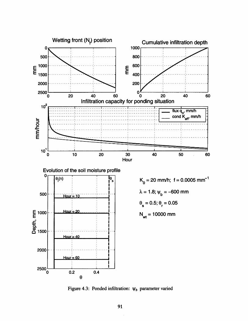
Wetting front (Nf) position
500
1000
1500
2000
2500
1000
800
600
400
200
Cumulative infiltration depth
Infiltration capacity for ponding situation
-. -.--. _..............cn K..........- ,od mm............................... .............. 1
. . .. . . . . . . . . . . . . . . . . . . . . . . . . . . .. . . . . . . . .
Hour
Evolution of the soil moisture profile
500
1000[-
1500 |--
2000-
0.2 0.4
K 0= 20 mm/h; f = 0.0005 mm-1
X = 1.8; 4b = - 600 mm
0 = 0.5; O = 0.05
N = 10000 mm
0
Figure 4.3: Ponded infiltration: yAb parameter varied
0,(n) S
...-..... ... ........ ...Hour:= 10
-..---.--.. ............ .....
Hour = 40
Hour =60
2500
-. . ...... . .. .............
-.. ....- .....-. .....
............ ~ ~ ~- .... ......
..
.. ....-. -.. .-.. .-.. .
-. ...... . . . . .
-. . . . . . . . . .
-. - - - - - -
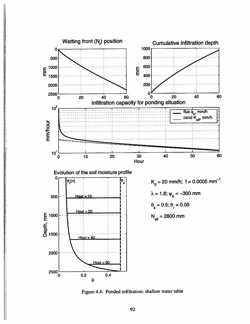
0
500
1000
1500
2000
250010 20 40
102
101
1000
800
600
400
200
Cumulative infiltration depth
--..... -.. .... -.. ...
-.....-. .. .........
-. .... -. ........-. ..
Infiltration capacity for ponding situation
Hour
Evolution of the soil moisture profile0,(n) : K =20mm/h; f=0.0005m
* I 0
500 ... .... Hour=10 ......... .... .. -- =: : I i n
Hou0 = 201000 -- - N 2800 mm
1500 -. .--- -
HoUr = 40
2000.............................20 0 - - - -I
2500I0 0.2 0.4
0
Figure 4.4: Ponded infiltration: shallow water table
fluxq , mmh. . . . . . . . . . . . .. . . . . - - - - - - - - -: - - - - - - - - - - - - -: -. o d K m___* cona Keff' mm/n............ ............... ..............
................ ........... ..............
Wetting front (Nf) position
-. ...... .....
-- . . . . .--------. . .. ..- ..
....:. . -. .....
-............-. ..-. .- -. .- - .- -
i

4.2 Test case: rainfall of constant and variable intensity
This section describes simulations of infiltration for the same hypothetical soil column
under conditions of rainfall with constant and variable intensity. The rainfall does not lead
to immediate surface saturation and therefore several transformations have to occur to the
soil moisture profile before runoff is produced (Section 2.1.2).
An example of the case when rainfall does not result in runoff generation is illus-
trated in Figure 4.5. A rainfall of intensity 4 mm/hour is applied to the soil with the follow-
ing hydraulic parameters: K0, = 10 mm/h, f = 0.001 mm 1, X = 1.8, 1b = -300 mm, 0,= 0.5,
and Or = 0.05. The water table is located at the depth 10 m. The top most plot in Figure 4.5
shows the rainfall intensity (mm/hour) and the plot below depicts the depth (mm) to the
wetting/top front during the simulation period. As seen, the rainfall does not lead to the
development of the perched zone and therefore the wetting and the top fronts coincide. The
third plot from the top illustrates temporal variation of the following variables: the infiltra-
tion flux rate q, , approximated by (2.19) of Section (2.1.2), the "equivalent" rainfall rate
Re, defined by (2.18) and equal to a constant unsaturated hydraulic conductivity K(0, Nf) for
the wedge of moisture above the wetting front Nf, and the saturated hydraulic conductivity
K,(Nf) estimated at the depth of the wetting front. The saturated conductivity always stays
higher than both the flux q, and the conductivity K(0, Nf). In agreement with an apriori
expectation, the redistribution flux q, asymptotically approaches its steady-state value equal
to the constant intensity of rainfall 4 mm/hour. The plot at the lower left corner illustrates
the states of the soil moisture profile corresponding to various times. The profiles are com-
puted according to (2.16).
Figure 4.6 shows results from another simulation corresponding to a 20-hour rainfall
event of 10 mm/hour intensity. The rainfall rate is high enough to create the perched zone
which starts developing at hour 11 at the depth of approximately 0.25 m. At this time, the
conductivity K(0, Nf ) of the moisture profile between the soil surface and the wetting front

is equal to the saturated conductivity at the depth of the wetting front K,(Nf ) and therefore,
according to (2.16), the soil moisture reaches its saturation value. Water accumulates above
that level and the perched saturation develops separating the wetting front from the top
front; the latter starts propagating upward. From that time, the conductivity K(0, Nf) in the
plot corresponds to the harmonic mean of the conductivities over the saturated thickness
formulated by the expression (2.25). The top front reaches the soil surface at about hour 16
and surface runoff production is initiated at this time, as seen in the top plot. The described
mechanism is typical for generation of saturation from below runoff.
Figure 4.7 illustrates soil response to rainfall of 20 mm/hour intensity. The forma-
tion of the perched zone at a very shallow soil depth almost coincides with the time of sur-
face saturation, at about 1.5 hour from the beginning of rainfall. Once the surface layer gets
saturated, the process is essentially described by equation (2.14) for the ponding case with
zero ponding depth. The flux or, in this case, the infiltration capacity q, decreases with time
as in the examples considered in Section 4.1. Runoff is generated during that time and the
overall process can be regarded as the Hortonian mechanism of runoff production.
An example of infiltration during a storm of variable intensity is given in Figure 4.8.
The soil parameters are the same. The first pulse of rainfall, hour 1-3, initiates infiltration
but does not result in runoff production. During the interstorm period, soil moisture redis-
tribution occurs leading to a significant surface soil moisture drop (the bottom left plot).
The second rainfall pulse, hour 42-28, slightly increases the redistribution flux and the soil
water content but is still insufficient to cause runoff generation. The third and the major
rainfall event between hour 57- and 67 has very high intensities that result in the develop-
ment of a surface saturated layer. The infiltration flux rate is lower than the rainfall rate and
therefore the runoff is produced (hour 58-61). After the rainfall intensity becomes less than
the flux q, , the soil moisture profile transforms to the perched saturated state (hour 61-62.5)
and eventually to the unsaturated state (hour 62.5-120). The soil water redistribution that
occurs after the rainfall ends drives the wedge of infiltrated moisture deeper. The average

soil moisture content decreases in the profile. The results of Figure 4.8 show consistency of
the soil moisture accounting scheme and its suitability for rainfall-runoff analysis in a
hydrologic model.
The results presented in Figure 4.9 are for the same storm pattern and soil type but
the water table is now located at a much shallower depth - 1.3 m. Accordingly, the initial
soil water profile is wetter and the soil's response to rainfall forcing is somewhat different
than that represented in Figure 4.8. The first two pulses of rainfall do not lead to runoff gen-
eration as in the case of initially dry soil. However, during the first 50 hours, the wetting
front penetrates to a deeper location, about 220 mm, as opposed to 170 mm for the initially
dry soil case. Consequently, during the third rainfall event, it takes slightly longer time to
reach surface saturation and the soil starts producing runoff at later time. The implication is
such that the total runoff produced by the initially wetter soil is less than that of the drier
soil: 66.6 mm as opposed to 73.1 mm. This is a counterintuitive fact on the surface. It
emphasizes the importance of soil moisture redistribution during past storm and interstorm
periods.
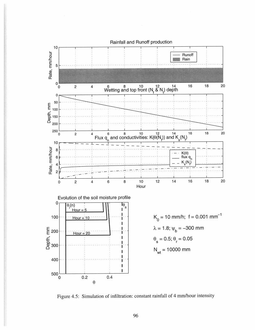
Rainfall and Runoff production
0 2 4 6 8 10 12 14Wetting and top front (Nf & N) depth
16 18 20
0
250--
100- --.-.-.-.
150 - -
200 2 4 10 12 14 16 18 21
Flux q and conductivities: K(O(Nf)) and K S(Nf)10
- I
0 2 4 6 8 10 12 14 16 18 20Hour
Evolution of the soil moisture profile0 (n) 10
Hour= 5
HcUw 10' K0 =10 mm/h; f =0.001 mm-
- .-. - - 1.8; 4b = - 3 0 0 mmHour-20d
0 = 0.5; 0 = 0.05S r
N =10000 MM
0.2 0.4
Figure 4.5: Simulation of infiltration: constant rainfall of 4 mm/hour intensity
96
- . .1 .. . . . . . . . . . . . . . . . . . . . . . . . . . . . . . . . . . . . . . . . ..
-- - K(O)...... ..... .....-..-.- flux q n
I ....... ........ . ... . . ... ... ... ..... . ... . . ... . K s (N ) . . . . . .
100
E 200
-C-
a) 30(
40
50
pI
0
0

Rainfall and Runoff production
i 10RunoffRain
5
00 2 4 6 8 10 12 14 16 18 21
Wetting and top front (Nf & Nt) depth0
1 0 0 -.. ......-. ............-. .. .-. ...-. ..-- --. ..- --- -
200 ............................
300 -
400-
500 I0 2 4 6 8 10 12 14
Flux q and conductivities: K(0(Nf)) and KS(Nf)16 18 20
.. .. . -. - - - - K(0) ...... . ......
.. . . . . .. K O
. . . .~.._ flux qns (N
0 2 4 6 8 10 12 14 16 18 20
Evolution of the soil moisture profileHour
K = 10 mm/h; f = 0.001 mm-1
X = 1.8; yb = -300 mm
0 = 0.5; O = 0.05s r
N= 10000 mm
0.4
Figure 4.6: Simulation of infiltration: constant rainfall of 10 mm/hour intensity
97
100
200-.
300 -
400
500
0,(n) 1sHour =3
Hour =7-
.Hour 14 - - .-.- .
Hour =20
0.2

Rainfall and Runoff production
-- RunoffMRain
0 2 4 6 8 10 12 14 16 18 21Wetting and top front (N & Nt) depth
1 1I
2 4 6 8 10 12 14 16 18 21Flux q and conductivities: K(0(Nf)) and K,(Nf)
0 2 4 6 8 10 12 14 16 18 20Hour
Evolution of the soil moisture profile
K0 = 10 mm/h; f = 0.001 mm1
X = 1.8; b = -300 mm
O = 0.5; O = 0.05
Nt = 10000 mm
0 0.1 0.2 0.3 0.4 0.50
Figure 4.7: Simulation of infiltration: constant rainfall of 20 mm/hour intensity
98
1 0 0 -- - - - - . -- - - - - - . . . . . . . . . . . . . . .-- - -. .- - - - -.-. .-- --. .- -.
20 0 -- .. --. --. .-. .--.
500
100
200
300
400
500
0 ()Hour 1 S
Hour=2 -- - - . - .
:. .. I
-. Hour#7 ----- ~
Hour= 14
Hour =20
--K(9). . .. ... . . .. . ... .. .lu X. .Ks(N)
0
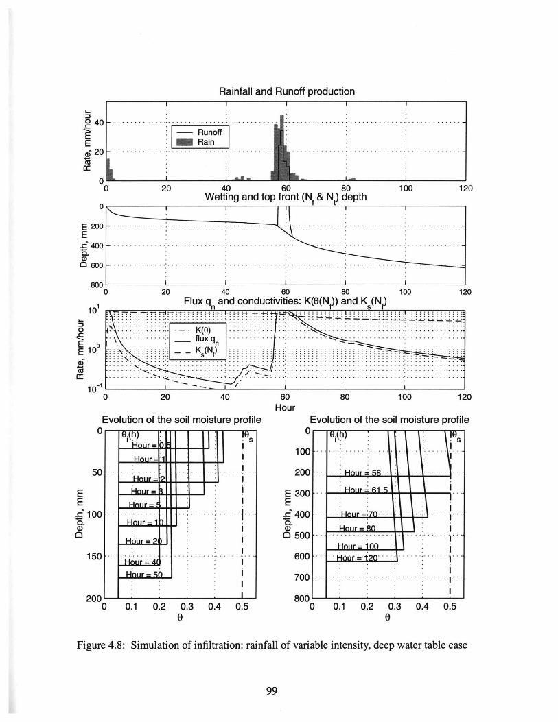
Rainfall and Runoff production
4 0 . .. . . . . . ................ . . . ..... ... ............. . .. .. ..... .............
-RunoffMRain
' 2 0 - . . . . . .-. . . . . . . . . . . .-- - - - - - - -- -.-- -. .- -.-- - .- - - - - - - - --. .- - --.- - -
0
0 20 40 60 80 100 1Wetting and top front (Nf & Nt) depth
0
2 0 0 . - - - -.-.-.-- - --.-.- -.-.-.-.-.-.-- - .-- - - - - - - - - .- -
600800' j0 20 40 60 80 100 12
Flux q and conductivities: K(O(Nf)) and KS(Nf)
-..._. flux gn -Z
NK __K(N ) -..-..-.-
10~100
Evolution of the soil moisture profile0 0.h 1
- . I .
5 0 -. . .. . .-. - -- --.-.-.-- - -.-- - -- -- -
EE
100 ...... -....- - . - .-
a1
...........
2000 0.1 0.2 0.3 0.4
00.5
120Hour
Evolution of the soil moisture profile0 0.(h) l S
100 ...- - - - - - - -......- -- -
200 . . ... -- -.............
E 300 --.E
400 = ... ........
C)
0500 ......... ...........
600 - Hor t2
700 .... :- -...... ...... ....
800'-0 0.1 0.2 0.3 0.4 0.5
Figure 4.8: Simulation of infiltration: rainfall of variable intensity, deep water table case
99
EE
CD
0
1
I 3
0
E oE 10CDIi
0
0

Rainfall and Runoff production
-- Runoff
Rain-. .... .-. ......-. .-.-
20 40 60 80Wetting and top front (Nf & N) depth
100 120
20 40 60 80 100 12Flux q and conductivities: K(0(Nf)) and Ks(Nf)
100Hour
120
Evolution of the soil moisture profile
0 0.1 0.2 0.3 0.4 0.50
100
200
300EE 400
.500
600
700
800
Evolution of the soil moisture profile
900'0 0.1 0.2 0.3 0.4 0.5
Figure 4.9: Simulation of infiltration: rainfall of variable intensity, shallow water table case
100
0 40
EE6i20cc
0
0
E 200E
400
0 6000
800
101
0
EE 10
10
-. .-. .-
. . ....-. .....I. .. . . . . . . . . . . . . . ..-. . .
.-- - - ..... ... : .....- .....- .....- . ....- ....- .....-
- - . . . . .- -. . .. . .-. .. .- --. . . . . .- -. . .. . .-. ..-
flux................... ................. ............................
. .. .. . ... . . . . . . . . . . . . . . . .
.... ... K N f) ... ... ...
100
150
200
250
0.(n) 10S..... .... ... ..
.. ...... ........
-. . - . . . ... .. ..

4.3 Ground water model off-line testing
The RIBS ground water model is based on the de-coupled 1-D formulation of Dupuit flow
as discussed in Section 2.3. Using cell-to-cell computation of volumetric fluxes, it has two
capabilities of ground water flow partitioning: the multiple and the single flow direction
algorithms. The first approach, referred as 'MS' in the following (after Tarboton, 1997),
allows for flow to all neighbors of the current element, in the direction of negative head gra-
dient. The maximum number of possible flow pathways is eight, which includes cardinal
and diagonal directions. The drawback of this approach (Costa-Cabral and Burges, 1994;
Tarboton, 1997) is that it results in a higher dispersion of the saturated flow. It was also
pointed out by the referenced authors that the "effective contour length", or a width normal
to the direction of flow, is chosen rather subjectively and for some cases may be wrong (for
instance, for ground water "saddle" nodes it is half of what it should be).
The second approach, referred as Doo in the following (after Tarboton, 1997),
allows to define an arbitrary angle of flow in a continuous 3600 plane (see Section 2.4, Fig-
ure 2.10-11). The flow may be partitioned between either one or two sides of the grid cell
(Figure 2.11). This depends on the value of the steepest slope of a plane through eight fac-
ets formed by the current and neighboring nodes (Figure 2.10, discussion is in Section
2.3.3). The numerical results are compared to the analytical solutions in order to evaluate
how well each of the partitioning schemes produces redistribution of the ground water.
4.3.1 Damping of a ground water mound in the infinite plane
Although the Dupuit approximation removes the non-linearity introduced by the presence
of a free-surface boundary condition, the resulting partial differential equation (the Bouss-
inesq equation, see equation (2.42)), describing the ground water flow is still non-linear
because of the product h ah . Exact solutions to the Boussinesq equation are possible foral
particular geometries and boundary conditions. Another approach to the problem would be
101

to linearize the Boussinesq equation (2.42). The simplest method used is to assume that the
thickness of the saturated zone h = h(x, y, t) varies only slightly in the domain of interest,
i.e. the assumption used in deriving equation (2.44). Assuming that the transmissivity is
homogeneous in the domain of interest, we can rewrite (2.44) with N = P = 0 in the form:
2 2-Ia h ahl ahT 2 + =h S, A (4.1)
ax ay 2
where the notation follows that of Section 2.3.
For two-dimensional flow in an infinite plane, Carslaw and Jaeger [1959] present a
solution for the linearized equation satisfying the initial conditions: t = 0, x I < L ,
|y I< L2, h = h, , with h = ho everywhere else, in the form:
h_-h_ L- L 1 + L2- L 2 +h = herf + erfl erf 1 +erf (4.2)
4 2a kt 2a ft J 2aft 2a (t
where a2 = T and the specific yield is assumed to be equal to the effective porosity, t isSY
time, and L, and L2 are the geometrical dimensions. Essentially, the problem is damping of
the ground water mound in the infinite plane (see Figure 4.10). The mound spreads out
without accretion and expression (4.2) defines deformation of the ground water free surface
with time.
Figure 4.10: Ground water mound
102

Using an off-line procedure, analytical distributions of the ground water surface are
obtained for various times using the following parameter set: K = 1 mm/hour, ho = 25 m,
h, = 27 m, S =0.5, L, = 15 m, L2 = 10 m. The RIBS ground water model (Section 2.3) with
the two alternative partitioning schemes (MS and Doo ) is employed to reproduce free water
table surfaces, for the same times and using the same parameter set. It should be noted, that
the partitioning schemes define the form of flux exchange between the adjacent grid nodes
while the ground water flow rate is controlled by the parameter a that is kept constant with
time as assumed by the linearized equation (4.1). Figures 4.11 and 4.12 show the spatial
distribution of the water table head for simulation run time 50 hours and 240 hours for the
MS and Do approaches respectively.
Figures 4.13 and 4.14 show the error surfaces of the estimated ground water levels
for both approaches for hour 50 and hour 150. The error surfaces are computed as the dif-
ference between the analytical and simulated head distributions. The range of error values
for the MS approach is [-7.65 cm, 6.52 cm] for hour 50 and [-4.2 cm, 9.25 cm] for hour 150.
The corresponding ranges for the Doo approach are [-9.06 cm, 0.6 cm] and [-4.46 cm, 1.83
cm]. As it can be seen, the MS approach results in higher dispersion of the ground water
flow producing larger range of errors which have considerable spatial variation. The figures
depict that this results in a slightly higher rate of ground water dampening with positive
errors (the head is lower than the predicted by the analytical model) concentrated along the
mound edges and corners. As it might be expected, the errors grow with time in these parts
of the mound producing four distinct positive "peaks" (Figure 4.14). The Doo approach
generally produces negative errors, i.e. the head is higher than the predicted implying a
lower dampening rate. Nevertheless, the error surface has less spatial variation and magni-
tude reflecting a more consistent estimates of ground water level distribution.
103
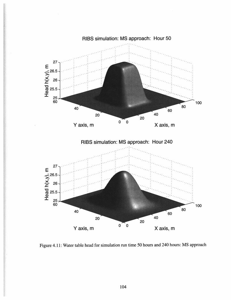
RIBS simulation: MS approach: Hour 50
27 -,
I.
80
Y axis, m 0 0
RIBS simulation: MS approach:
Y axis, m S0
X axis, m
Hour 240
X axis, m
Figure 4.11: Water table head for simulation run time 50 hours and 240 hours: MS approach
104
E.26.5 -
26-4
cd 25.5 -
25.60
27,E
26.5 -
26
ci 25.5
25>60 100
80
100

RIBS simulation: Doo approach: Hour 50
AA 80
Y axis, m0 0
4020
X axis, m
100
RIBS simulation: Doo approach: Hour
-A
100
Y axis, m0 0
4020
X axis, m
Figure 4.12: Water table head for simulation run time 50 hours and 240 hours: Doo
approach
105
27,E
26.5
X 26-
U 25.5
2560
240
27- -
E26.5 -
26-
C 25.5 -CD)
25 2
60

Error surface: analytical - RIBS simulation h(xy) (MS approach): Hour 50
Y axis, m X axis, m
Error surface: analytical - RIBS simulation h(x,y) (Dx> approach): Hour 50
Y axis, m
01
-10 -15 -10X axis, m
Figures 4.13: The error surfaces: Hour 50
106
0.1
E 0.05
0x
-0.05
-0.110
E 0.05
0-x
<-0.05
-0.110
-10 EW -15
0.1 -1 -
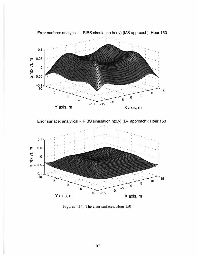
Error surface: analytical - RIBS simulation h(x,y) (MS approach): Hour 150
0.1- -
E 0.05-
<i -0.05,
-0.110
Y axis, m -10 -15 X axis, m
Error surface: analytical - RIBS simulation h(x,y) (Do approach): Hour 150
Y axis, m X axis, m
Figures 4.14: The error surfaces: Hour 150
107
*1**E
0-x
<-0.05 -
-0.110
0.1 - -
5 .. - . . -- .- 10
-5 -5
-5 -10 -15 -10 -

4.3.2 Instantaneous filling of a canal: semi-infinite case
The ground water flow in the case considered above has unusual flow symmetries and
results in a distribution of the ground water free surface that has a symmetric form. At the
beginning of the simulation, one can observe eight dominant directions of the ground water
flow: four in the cardinal and four in the diagonal directions of the projection of the mound
on xy plane made at t = 0. They are approximately constant until the mound has sufficiently
dampened such that there is no particular dominant direction and the number of principal
flow directions becomes infinite (Figure 4.11, the plot for hour 240). It is useful to consider
a problem in which a dominant ground water flow direction exists and changes with time.
Polubarinova-Kochina [1952, 1962] presents the solution of equation (4.1) for the
flow in a semi-infinite plane y 0 , where for t 0 , h(x, y, 0) = f(x, y) and h(x, 0, t) =
F(x, t) in the form:2 2-
1 (FF x- ) +(-h(x, y, t) = 2__ d+((y,-r)exp2_
-00 0 (43)
- exp - )2 +(y+ ) d + y2d TF( T ,e (x - + 1dex4a2t I4 a 2 _ (t - ) _2 4a 2(t - ) _
Polubarinova-Kochina [1952, 1962] considers a canal with vertical walls and impervious
bottom. At the initial moment of time, the ground water level is at a constant HO. Suddenly
the canal is filled so that in one of its parts, for x < 0, the water level is H1 , and in the other
part, for x > 0, the water level is H2. These levels are then kept constant. The solution is
searched for the upper half space (y > 0). In this case:
f(x, y) = H0, F(x,t) = {H1, for x<0
H 2, for x > 0
After transformations, Equation (4.3) becomes (Polubarinova-Kochina 1952; 1962):
h(x, y, t) = HOb 2 + H; +H 2 [ 1 - (b2( -
(H 1 -H2 2_ 2-_d_(- exp - ] 2 (4.4)01 - 4a 2t _n + y2
108
where (D i is the error function:2a~t
CD = 1 2ye 1 + y2 ] di12at 0 -4a 2t _1 + y2
The function h(x, y, t) in Equation (4.4) is composed of three terms: the first is derived from
the initial ground water level, the second corresponds to the homogenous problem with con-
stant head 0.5(H + H2), and the third, depending upon x, determines the asymmetrical flow
due to the difference in head between head- and tailwater.
Simulation runs were carried out with the following set of parameters: K = 5 mm/
hour, Ho= 25 m, S, = 0.5, H, = 26 m, H2 = 27.5 m. The plots in Figure 4.15 show the
ground water free surface for hour 240 as simulated by RIBS using the two flow partitioning
schemes. Contrary to the previous case of dampening of ground water mound, positive
error means that the simulated head is higher than the one obtained analytically. Hence,
positive errors correspond to a higher ground water flow rate, as long as in the domain of
interest head values increase with time. Figures 4.16 and 4.17 show error surfaces com-
puted for different times from the start of simulation. The range of error values for the MS
approach is [-2.27 cm, 18.2 cm] for hour 50 and [-3.38 cm, 17.9 cm] for hour 240. The
mean errors estimated for these times are 2.79 cm and 6.09 cm. The corresponding error
ranges for the Doo approach are [-17.8 cm, 6.8 cm] and [-20.1 cm, 6.67 cm], with average
errors equal to 0.88 cm (hour 50) and 1.82 cm (hour 240). As in the previous comparison,
the Doo flow partitioning approach results in a less erroneous and more consistent ground
water level distribution. Except for a few points of extremely high gradient where it tends
to underestimate heads (Figures 4.16, 4.17), the Doo approach produces quite reliable
results compared to the analytical case. The MS approach generally overestimates fluxes
throughout the whole domain and the error grows in magnitude and spatially expands with
time. Overall, the Doo approach performs better than the MS approach which tends to
accumulate errors during simulation.
109

RIBS simulation: MS approach: Hour 240
27.5-
E 27--
26.5 -x
26-a>I25.5 -
2540
20
-20 s m20
Y axis, mA ais, I II
RIBS simulation: Doo approach: Hour 240
27.5
E 27 .
>'26.5
26-CO
3 25 .5 -
25:240
20
-20
X axis, m
Figure 4.15: Water table he
............ 10................... 2 0
30-40 40
Y axis, m
id for simulation run time 240 hours: both approaches
110

Error surface: RIBS simulation (MS approach) - Analytical: Hour 500.2 .
0.1
0
0.1 . ............ ........... .
0
......................20
2 0 -.---.- 5-.
-20 -- - ,-- --- , ---- ~-
An 1n s 0
X axis, m Y axis, m
Error surface: RIBS simulation (Do approach) - Analytical: Hour 50
3.2 -...
I ..... ...... ....
0 .2 .. . . .. .. . ...
00 - -.. .... . . -..-..--...-..-
-20 -
c -IA n 0
X axis, m Y axis, m
Figures 4.16: The error surfaces: Hour 50
111
E
x-c
-
4

Error surface: RIBS simulation (MS approach) - Analytical: Hour 240
0.2
E
x
X axis, m Y axis, m
Error surface: RIBS simulation (Do approach) - Analytical: Hour 240
E 01x
-0.1
-0.240
20
0
-2
X axis, m
0... -
0 .
-4040 35
Figures 4.17: The error surfaces: Hour 240
112
25 20
Y axis, m
10 5
-. .....-. . .. . .
..............
-. - - - -. .
. . .-.
CHAPTER V
Model Performance: On-line Model Applications
Two applications of the RIBS model are presented in this chapter. A synthetic hillslope
model is used to demonstrate the model's capability to simulate the principal phases of
hydrologic response in a system that couples the unsaturated zone and the ground water.
The mid-sized Peacheater Creek basin (OK) is used to test the model behavior in an actual
watershed with the NEXRAD Stage III data used as rainfall input.
5.1 Test case: the hillslope model
A synthetic hillslope model has been created to test the validity of the parameterizations
described in the preceding chapters. The one-dimensional hillslope is composed of 100
3000 m x 30 m elements in which the slope vector is perpendicular to the longer side. The
right-most pixel in Figure 5.1 (at the distance 3000 m) is the hillslope outlet, or a stream
node. As it can be seen in the top plot of Figure 5.1, the topography of the hillslope com-
bines both features of convexity (the upper part) and concavity (the lower part). These char-
acteristics will allow one to evaluate how realistically the model simulates infiltration and
subsurface lateral exchange in the corresponding hillslope areas. The bedrock depth is
assumed to be uniform along the hillslope and is assigned to the depth of 10 m. The second
plot from the top shows the variation in surface slope along the hillslope.
A parameter sensitivity study has already been presented by Garrote [1993] and
Rybarczyk [2000]. In the current test, the emphasis is on the model's potential to consis-
tently simulate dynamics of the hydrologic variables under different meteorologic condi-
tions. Two basic scenarios of the hillslope initial state are considered: initially wet and dry
conditions. The corresponding depth to the water table is shown in the bottom plot of Fig-
ure 5.1. The following analysis of the hillslope response to a sequence of various meteoro-
113

logic forcings starts for the wet case with the following parameter set: K0, = 10 mm/h,
f= 0.0007 mm 1, X0 = 2.0, yb = -200 mm, OS = 0.5, Or = 0.05, and ar = 100.
5.1.1 The wet case
Figure 5.2 illustrates the cross-sectional view of the hillslope after applying spatially uni-
form rainfall of 1 mm/hour intensity for 11 hours. The plot shows the hillslope topography,
the initial (before simulation) and the simulated position of the top of the saturated zone, the
wetting and the top fronts. Several remarks must be given regarding some of these variables
and the scale at which they are depicted.
The shown top of the saturated zone is in fact the top of the capillary fringe zone
that has a negative capillary pressure according to the parameterization introduced previ-
ously (Section 3.2). Thickness of the capillary fringe zone is defined by the parameter Wb,
the air entry bubbling pressure (Section 3.2). At the bottom of this zone, the pore water
pressure is zero which determines the water table.
Scales at which the variables are depicted are different. The actual elevation (in) is
shown only for the hillslope topography but the Y-axis in both the top and bottom plots (e.g.
Figure 5.2) has a larger scale than the X-axis. Vertical exaggeration is used to help in visu-
alizing the position of the fronts in the unsaturated zone and the top of the saturated zone.
The corresponding vertical exaggeration factor for their depth is specified in each plot. For
example, if the actual wetting front depth is 0.1 m and the vertical exaggeration factor is
equal to 15, the wetting front is shown as located 1.5 m below the land surface.
The top plot in Figure 5.2 illustrates the overall hillslope cross-sectional profile
while the bottom plot shows only the lower part of the hillslope which is the most dynamic
during a storm event in terms of changes in the unsaturated and saturated zones. The legend
for both the top and bottom illustrations is given in the top plot. The top front and the wet-
ting front are shown as dash-dot lines and if their simulated positions coincide, only a single
line is depicted (bottom plot in Figure 5.2, Figure 5.3). If the fronts do not coincide (i.e. a
114

perched zone exists, as will be shown later in Figure 5.5), then the lower dash-dot line
depicts the position of the wetting front and the top line illustrates the top front location.
The same remark can be made for the location of the top of the saturated zone: if its final
position almost coincides with the initial (i.e. the one at the beginning of simulation), then
only the final location of the top of the saturated zone is shown (thick solid line, e.g. bottom
plot of Figure 5.2, pixels #50-76). If its final position is different enough from the initial
location, then the initial depth of the top of the saturated zone can be distinguished in the
illustration (thick dashed line, e.g. bottom plot of Figure 5.2, pixels #77-84).
The middle plot in Figure 5.2 shows the simulated wetting and top front depth along
the hillslope without the vertical exaggeration. The thin solid line represents the wetting
front position and the dash-dot line depicts the location of the top front. As above, if the top
and wetting front coincide along the hillslope, only the wetting front depth is shown
(Figure 5.2). As it can be seen in the plot, the depth to the wetting front varies in different
parts of the hillslope with a slightly thinner unsaturated wedge in the steep slope area at the
hillslope top (starting at a distance 350 m) and a thicker wedge in the lower concave part.
As it will be shown, this variation becomes more pronounced at later times. The explana-
tion of the wetting front location at the hillslope bottom (at a distance > 2300 m) is given
below.
The bottom plot in Figure 5.2 illustrates that some changes have occurred in the sat-
urated zone in pixels #77-83. As seen, the wetting/top front in pixel #77 at a distance of
-2300 m (in the middle plot it is where the line goes down to 200 mm) is at the depth of the
saturated zone which means that the wave of infiltrated water has already reached the top of
the capillary fringe. According to the assumptions made in Section 2.2.1, once the wetting
front reaches the top of the saturated zone, its location is then assigned to the water table.
No new infiltration moisture wave is initiated while the rainfall conditions persist. Any sub-
sequent amount of moisture coming into the cell is redistributed in the soil moisture profile
(example of this is given in Figure 2.9). Pixels #77-81 (in the distance range between
115
-2300-2400 m) illustrate this parameterization. Such redistribution occurs until the pixel
becomes completely saturated (as in the pixels #82-83) and the wetting front is then
assigned to the land surface (in the middle plot of Figure 5.2 this corresponds to the distance
> 2400 m). According to this discussion, the change of the water table position in pixels
#77-83 is therefore a combined effect of the described above unsaturated zone dynamics
and the ground water flow. In general, because pixels #82-100 are in a completely saturated
state, they generate the saturation from below and ground water flow.
Figure 5.3 illustrates distribution of the same variables after an 18-hour no-rainfall
period that followed the 1 mm/hour rainfall event discussed above. As it can be seen in the
middle picture, while the redistribution occurs in the moisture profile, the wave of infiltrated
water penetrates to a deeper location along the hillslope compared to the results in
Figure 5.2. The convergence of moisture at the hillslope bottom becomes a bit more pro-
nounced at this time. One can also notice that a break point in the profile of the wetting
front depth (at a distance -350 m). This point corresponds to a sharp change in the hillslope
topography where the surface slope increases up to 200 (Figure 5.1). Moisture tends to
migrate from that point which is reflected in a slightly shallower wetting front depth with
respect to pixels in a flatter top hillslope area. As long as some part of the hillslope bottom
is still in the saturated state, ground water flow is generated.
Changes in the saturated and unsaturated zone resulting from simulation of evapora-
tion conditions are shown in Figure 5.4. After the no-rainfall period discussed above, a 16-
hour period of evaporation of 1 mm/hour intensity is modeled as negative moisture flux at
the soil surface. At the beginning of this period, the moisture leaving the soil due to evapo-
ration is extracted from the profile of infiltrated water. By the end of the period, once the
moisture excess in the unsaturated zone has been evaporated, the water for subsequent evap-
oration is extracted directly from the hydraulic equilibrium profile corresponding to the
present ground water position. The ground water level goes down to conserve mass. The
bottom plot in Figure 5.4 shows that the water table has dropped as a result of the applied
116
evaporation conditions. At the hillslope bottom (pixels #82-100), the ground water table
went down from the soil surface. Correspondingly, once the unsaturated zone does not con-
tain the wave of infiltrated water anymore, the wetting/top front can be assigned either to
the land surface (pixels #1-63 or up to the distance -1850 m) or to the top of the saturated
zone (pixels #64-100, distance > 1850 m). This is defined based on the previous infiltration
history of a pixel. The position of the wetting front is assigned to the land surface if a pixel
transitions from an unsaturated, perched or surface saturated state (these states are illus-
trated in Figure 2.4). In these three cases the wetting front of the wave of infiltrated water
has not reached the top of the saturated zone. This is the case for pixels #1-63. The wetting
front is kept at the top of the saturated zone if a pixel transitions from a fully saturated state
or an equilibrium moisture state where the wetting front has already been assigned to the
top of the saturated zone (pixels #64-100). For the latter situation, the wetting front has to
be re-assigned to the land surface level at some point after the beginning of a no rainfall
period. Recalling from Section 2.2.1, it is assumed that after a given time with no rainfall
the interstorm period begins and any following storm will generate a new wave of infiltrated
water. The required condition for that to happen is a period of no rainfall which has to
exceed a certain threshold value of time. Because in this case the value has not been
exceeded, it is assumed that the system is in a dry interval within an on-going storm and the
wetting front remains at the top of the saturated zone for the pixels #64-100 in Figure 5.4.
The evaporation event discussed above is next followed by a 16-hour period of rain-
fall of 10 mm/hour intensity. Figure 5.5 illustrates the simulation results corresponding to
the 14th hour of that period. As it can be observed, a perched zone has developed along the
hillslope as a result of rainfall which has a high intensity relative to the soil surface conduc-
tivity. As indicated above, the upper dash-dot line in the top plot illustrates the location of
the top of the perched zone (the top front) along the hillslope while as the lower dash-dot
line depicts the bottom of the perched zone (the wetting front) position.
117

The break point in the profile of the wetting and top front depth at a distance -350 m
is clearly pronounced at this time. As referred above its formation is caused by significant
slope of the hillslope topography (Figure 5.1) which leads to the destruction of the perched
zone at that pixel. As seen, the perched zone is also less developed in the surrounding area.
In general, the perched zone is less developed in the steeper topography area at the top of
the hillslope and has a larger thickness at the hillslope bottom. Such observation is consis-
tent with apriori expected moisture divergence from the relief forms having higher topogra-
phy gradient and a general tendency for moisture to accumulate in the concave regions.
At this time about 28 elements at the hillslope bottom are completely saturated with
the top of the saturated zone located at the soil surface. These elements produce the satura-
tion from below and ground water flow runoff. In the next two hours of the rainfall period
(not illustrated), some fraction of the hillslope perched layer reaches surface saturation and
generates runoff as a result of limited soil infiltration capacity. In the context of the model,
the runoff is referred to as "Hortonian" to indicate runoff generation due to a rainfall rate in
excess of the redistribution flux of the saturated perched layer.
Figure 5.6 shows the cross-sectional view of the hillslope after the last simulation
period, a 10-hour period of evaporation of 3 mm/hour intensity. One can observe that while
the redistribution occurs in the moisture profile, the wave of infiltrated water transitions
from the surface/perched saturated state to the unsaturated state. As in the above examples,
while the moisture excess in the unsaturated zone is enough to support the evaporation flux,
the moisture wedge is not destroyed. Once the pixel transitions to an initialization state, the
moisture extraction occurs from the initialization profile and the water table goes down to
conserve mass.
The sequence of rainfall and evaporation events as well as the produced runoff are
shown in Figure 5.7. The bottom plot is the hillslope hydrograph, the runoff generated at
different locations in the hillslope and routed to the outlet (pixel #100). The plot in the mid-
118
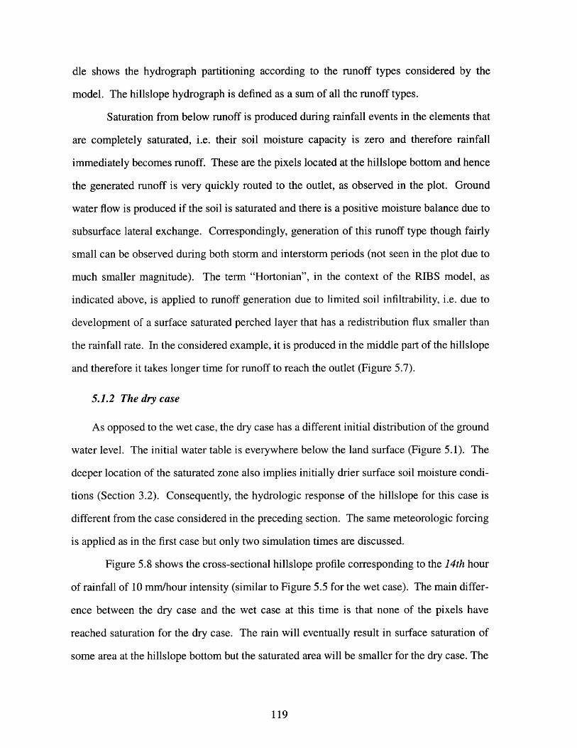
dle shows the hydrograph partitioning according to the runoff types considered by the
model. The hillslope hydrograph is defined as a sum of all the runoff types.
Saturation from below runoff is produced during rainfall events in the elements that
are completely saturated, i.e. their soil moisture capacity is zero and therefore rainfall
immediately becomes runoff. These are the pixels located at the hillslope bottom and hence
the generated runoff is very quickly routed to the outlet, as observed in the plot. Ground
water flow is produced if the soil is saturated and there is a positive moisture balance due to
subsurface lateral exchange. Correspondingly, generation of this runoff type though fairly
small can be observed during both storm and interstorm periods (not seen in the plot due to
much smaller magnitude). The term "Hortonian", in the context of the RIBS model, as
indicated above, is applied to runoff generation due to limited soil infiltrability, i.e. due to
development of a surface saturated perched layer that has a redistribution flux smaller than
the rainfall rate. In the considered example, it is produced in the middle part of the hillslope
and therefore it takes longer time for runoff to reach the outlet (Figure 5.7).
5.1.2 The dry case
As opposed to the wet case, the dry case has a different initial distribution of the ground
water level. The initial water table is everywhere below the land surface (Figure 5.1). The
deeper location of the saturated zone also implies initially drier surface soil moisture condi-
tions (Section 3.2). Consequently, the hydrologic response of the hillslope for this case is
different from the case considered in the preceding section. The same meteorologic forcing
is applied as in the first case but only two simulation times are discussed.
Figure 5.8 shows the cross-sectional hillslope profile corresponding to the 14th hour
of rainfall of 10 mm/hour intensity (similar to Figure 5.5 for the wet case). The main differ-
ence between the dry case and the wet case at this time is that none of the pixels have
reached saturation for the dry case. The rain will eventually result in surface saturation of
some area at the hillslope bottom but the saturated area will be smaller for the dry case. The
119

smaller saturated area implies a lesser contribution by the saturation from below and ground
water flow runoff.
Figure 5.9 corresponds to the end of the last period (Figure 5.6 for the wet case).
The observation one can make is that the hillslope bottom in this case is consistently drier
than in the case presented in Figure 5.6.
The hillslope hydrograph is given in Figure 5.10 and as expected the volume of sat-
uration from below runoff is much smaller than in the wet case and comparable to the vol-
ume of "Hortonian" runoff. A conclusion is that in the dry case it takes much more time to
saturate the hillslope to the point where runoff could be produced.
120

General hillslope representation
200 .................... ........ TopographyBedrock
0 I500 1000 1500 2000 2500 3000
Slope of the hillslope
500 1000 1500 2000 2500 3000
Depth to ground water and bedrock along the hillslope
-.-.-.-.-. -. .-.-.-.-.- .-.-.-.-.-.-.
7 Ground water: Wet case~- - Ground water: Dry case
-....------ - Bedrock depth
500 1000 1500 2000 2500 3000m
Figure 5.1: Representation of an artificial hillslope
121
25 -
20-
o 15-0.
C5 10 -
5-
00
0
2000
4000
6000
8000
10000
.................
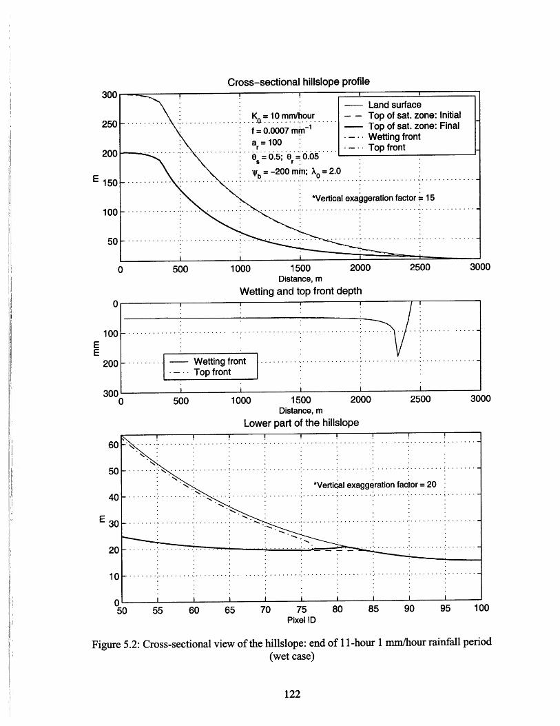
Cross-sectional hillslope profile300 _7
Land surfaceK = 10 mm/hour - - Top of sat. zone: Initial
2 5 0 ......... ...... .. ...... .250----- f-=007 --- Top of sat. zone: Final
a -00 - Wetting front
200a.................... = 0-...... -- Top front20 0 .5 0.05
E o 200 min; XO= 2.0150 -.. .. .- - 0 -
*Vertical exaggeration factor 151 0 0 - . . . .. . .-. .-. . .-...-.
.-. .-
50 - ..- . -.-.-
0 500 1000 1500 2000 2500 3000Distance, m
Wetting and top front depth0
100 - .-- - -. :. ~
EE
200 -. - ~.-. - W etting front -.-.-.-.-.-.-.-.-.-.-.-. -.-.-.-.-.-.-.-.-.-.-.-.-.-.- -
- Top front
3000 500 1000 1500 2000 2500 3000
Distance, mLower part of the hillslope
60 - :
50 .......*Vertica exaggeration factor = 20
40. --.-.-. ~
2 0 - -. .. . -... -. ..-.
050 55 60 65 70 75 80 85 90 95 100
Pixel ID
Figure 5.2: Cross-sectional view of the hillslope: end of 11-hour 1 mm/hour rainfall period(wet case)
122

Cross-sectional hillslope profile
: KQ =10 mm/bour-. .-. .-. .-. .
a = 100 Wetting front... . ... -.- . .. ... .............. Top front
0= 0.5; 0r = 0.05
- b = - M- ; A = 2.0
*Vertical exaggeration factor 15
- -:
500 1000 1500Distance, m
2000 2500 3000
Wetting and top front depth
- -Wetting front ..............Top front
500 1000 1500Distance, m
2000 2500 3000
Lower part of the hilislope
*Vertical exaggeration factor = 2040 - --- ----
E 3 0 - .. -.-.-.-.---.-- --.--.-.-
2 0 - ---..... ---.-..- - -
1 0 - - --. ... . . ... . . .--. . . . . .. .. . . .--. .-. .- -.-. .-- -..-.- -. .-. .-- -
55 60 65 70 75Pixel ID
80 85 90 95 100
Figure 5.3: Cross-sectional view of the hillslope: end of 18-hour no-rainfall period(wet case)
123
30C
250 F
Land surface- - Top of sat. zone: Initial- Top of sat. zone: Final
200
E 150
100
50
0
100
200
300
--
50

Cross-sectional hillslope profile
K =10mm/hour. ..........S f 0 _J I
= 0.0V 0 mmI
a = 100-- Wetting front........................ -- Top front
08=0.5; 0r= 0 .05
4b =-200 mm; ). = 2.0
*Vertical exaggeration factor 15
.. . .. . . . . . . . . . . . . . . . . . . . .
1000 1500Distance, m
2000 2500 3000
Wetting and top front depth
-.-.-.-- Wetting front............Top front
-- -.-. -
1000 1500Distance, m
2000 2500 3000
Lower part of the hillslope
*Vertical exaggeration factor = 20- . . . .. .. . . . -. -.. .. .. -.. . . . . -. . . -. . ... . . . . . .
- - - -. . ..-. .. .-.- -. .- . -. .- -.
0'-5 0) 55 60 65 70 75 80 85 90 95 100
Pixel ID
Figure 5.4 Cross-sectional view of the hillslope: end of 16-hour 1 mm/hour evaporationperiod (wet case)
124
300
250 F
Land surface- - Top of sat. zone: Initial
- Top of sat. zone: Final
500
0
200
400
600
800
0) 500
50
40
E 30
101 -. - - . . -
I I
I .

Cross-sectional hillslope profile
: KQ =10 mm/hour. . . -.
a 100 - Wetting frontar .... - Top front
- s=0.5; 0r= 0.05
-4b =-20 min; O = 2.0. . . . . .. .. . . . . . . . . . .. .. . . . e. . . . ......e ..e .- e .e .
*Vertical exaggeration factor:: 15
. . . .. ~ . . . . . . . . . . . . . . . . . . . . . . . . . . . . . . .
500 1000 1500 2000 2500Distance, m
Wetting and top front depth
. .., ~ . - - . . . . . .. . . . -
............ ........................... ........... ........... .......... ....
-.. .- ......- ...-.....- . . - . - - --- W etting front- -- Top front
500 1000 1500 20Distance, m
Lower part of the hillslope
00 2500
3000
3000
55 60 65 70 75 80 85 90 95 100Pixel ID
Figure 5.5: Cross-sectional view of the hillslope: end of 14th hour of 16-hour 10 mm/hourrainfall event (wet case)
125
Land surface-- Top of sat. zone: Initial
-- Top of sat. zone: Final
300
250
0
200
400
600
20
10
nA1
*Vertical exaggeration factor = 20
- -- -. -.- - - - -.- - - --.-.-.- -.- -.-.-.-. -
.....- ---. . - --.. .. - -.. . -.. .. -.. .. -.. .. -.. .. -. ..
- - - - - - - - - - - - - - - - -. .
-.. -. -. . -.
E 30
50

Cross-sectional hillslope profile
--- Land surface.- K... = 10 mm/hour - - Top of sat. zone: Initial
0.0007 mm~ - Top of sat. zone: Final
100 Wetting front-- . -- - - -- - - --..... aT= 1 .....:......... - - - T op front
- 0 =0.5; 0 =0.05
- y = -200 mm; X = 2.0
*Vertical exaggeration factor 15- - - - - - - - - - - - -. - - - - -. . . . . . . . . . . . .
- - - -. . . . . . . . . . . . . . . . . . . . . .. . . . . . . . . . . . . . . . . .
500 1000 1500Distance, m
2000 2500 3000
Wetting and top front depth
SWetting front
----Top front
500 1000 1500 2000 2500Distance, m
Lower part of the hillslope
*Vertical exaggeration factor = 20
INI
- -.. .. . - . . . -.. . . . . . . --.. . -.-. .-. .-
- . . . ... . .- . - . . .. . . . .. . . .-. .. .-. ...-. . ..-. ...-.
3000
55 60 65 70 75 80 85 90 95 100Pixel ID
Figure 5.6: Cross-sectional view of the hillslope: end of 1 0-hour 3 mmn/hour evaporationperiod (wet case)
126
300
250
200
E 1501
100
50
200
400
600
At
50
40
E 30
10

Meteorological forcing
Total Rain =171 mmTotal Evap 46 mm
10 20 30 40 50 60 70 80
Simulated Runoff Types
10 20 30 40 50 60 70 80
Simulated hydrograph
10 20 30 40 50 60 70 80Time, hour
Figure 5.7: Hyetograph and hydrograph for the hillslope simulation (wet case)
127
Sat. from below-- "Hortonian"
-- Perched Saturation- - Groundwater flow
8
6
4E
8
7
6
5
CO
3
2
1
0
0.0007 mm- Ksat 10 mm/h;
ar =100; Uar =100; X= 2 (c =4)
b =-200 mm;0 =0.5;0 =0:05
-..-- C =0.75 rn/h (=075 m/)....
- vh
Exp r 0
- Simulated ruroff 39.5086
........ ................
..........
........... .
.............F
2 r -. . . . . . .
. . . . . . . . . . . . . . . . . . . . . . . . . . . . . . . . . . . . .
. . . . . . . . . . . . . . . . . . . . . . . . . . . . . . . . . . . .
. . . . . . ... .. . . . .. . .. . . . . . . . . . ...........
......... ........... .......... .. .......
............... ............ . . . . . . . . . . ..
........... ..........mm
....... ..........

Ij
KQ =10 mm/hour.f A A -
300
250
200
150
100
50
1000 1500Distance, m
2000 2500 3000
Wetting and top front depth
1000 1500Distance, m
2000 2500 3000
Lower part of the hilislope
50
40
A I
55 60 65 70 75 80 85 90 95 100Pixel ID
Figure 5.8: Cross-sectional view of the hillslope: end of 14th hour of 16-hour 10 mm/hourrainfall event (dry case)
128
Cross-sectional hillslope profile
-~ I~E
S= 100- - - Wetting frontar = 100Top front. r ......... .: . . . . - - T p r n0 = 0.5; r=0.05
b =b-200 mm; -2.0
*Vertical exaggeration factor 10....................................... ...........
.............................................
Land surface- - Top of sat. zone: Initial
-- Top of sat. zone: Final
500
0
200
400
600
. . . . . . . . . . . .
............
Wetting frontTop front
500
*Vertical exaggeration factor = 1-.. ... ..
............ . .......
I . . .. :... .. . .
. .. ... ....... ... .. .... . . . . ........
I I I77.
I
0:
10
50
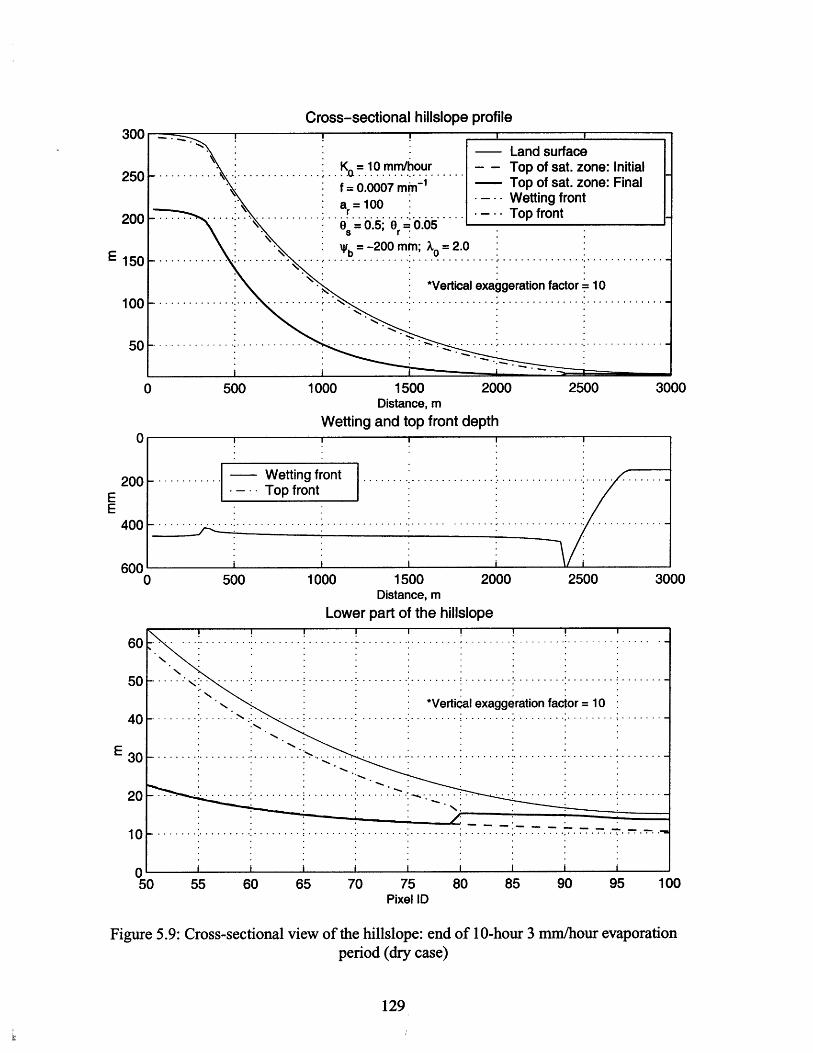
Cross-sectional hillslope profile
-Q =10 mm/hour. . I.I........1.. ..
a=100 : . -II Wetting front- =0..--.-.-.-.-..r ...... Top front
0 0.5; r=00r
b=-200 mm; X 2.0
*Vertical exaggeration factor 10- ..- . . . .-. -. . . . .-. . . . .-. .-.-.-.-.-..-- --.-.-.-
- - -- -.. . . . . ..-. - --...- - .. .- - ..- ..-
1000 1500 2000 2500 3000Distance, m
Wetting and top front depth
-.-.. -.. - Wetting frontTop front
-.. ...... ................. -.. .. ..............
1000 1500 2000 2500 3000Distance, m
Lower part of the hillslope
*Verti al exaggeration factor = 10
- -- - -- - - - - - --. . . .. . .--. ... . . .-.-- - -.-- ---..- -.-- -.--.-.
55 60 65 70 75 80 85 90 95 100Pixel ID
Figure 5.9: Cross-sectional view of the hillslope: end of 10-hour 3 mm/hour evaporationperiod (dry case)
129
300
250 l-
Land surface- - Top of sat. zone: Initial
- ToD of sat. zone: Final I
500
200
E 150
100
50
0
200
400
600
IL
500
.'
- . . . .- - - - - - - .- -
50
40
E 30
10
050

Meteorological forcing
: Tota Rain 171 mm
Tta Evap =46 mm
i- - - - - - - --
10 20 30
Simulated40
Runoff70 8050
Types
10 20 30 40 50
Simulated hydrograph
- -. Ksat 10 mm/h; 0.0007 mm - -
a 100; Ua 100;. .=2 (E=4)
- b*- r2c0 mm;.OQ= 0 ~ 0 .05
- v 0.75 rn/h.(=0 75 m/s).
Expr=0- .-..........................----..-.-.----.-.---.-.-
Simulated runoff: 1.605 mm- .- .-.- . - - . - . - .- - .- .-.-
-~~. ....-.- -. .- -. .- -. .- -. .-- .
60 70
10 20 30 40 50 60Time, hour
70 80
Figure 5.10: Hyetograph and hydrograph for the hillslope simulation (dry case)
130
0
2.
Sat. from below- "Hortonian"
- - Perched Saturation- Groundwater flow
0.5 [-
2
1.8
1.6
1.4
1.2
1
0.8
0.6
0.4
0.2
...........
G
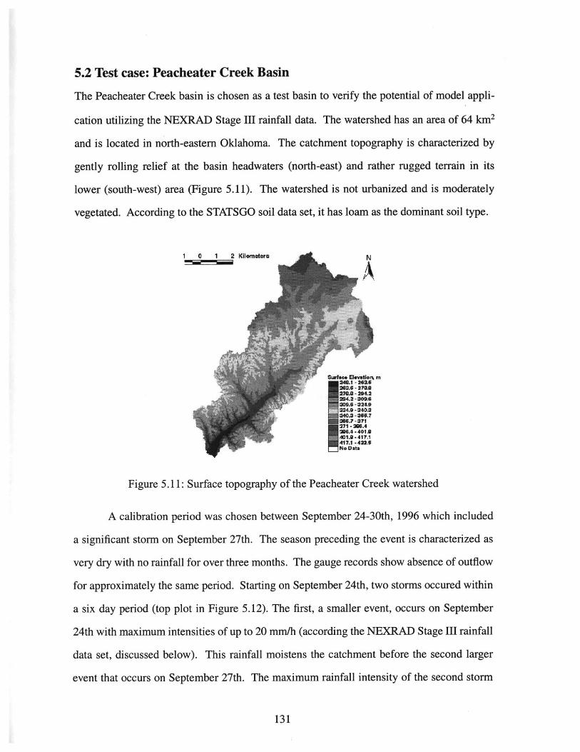
5.2 Test case: Peacheater Creek Basin
The Peacheater Creek basin is chosen as a test basin to verify the potential of model appli-
cation utilizing the NEXRAD Stage III rainfall data. The watershed has an area of 64 km2
and is located in north-eastern Oklahoma. The catchment topography is characterized by
gently rolling relief at the basin headwaters (north-east) and rather rugged terrain in its
lower (south-west) area (Figure 5.11). The watershed is not urbanized and is moderately
vegetated. According to the STATSGO soil data set, it has loam as the dominant soil type.
1 0 1 2 Ki omsteN
271 -26.4
=6.4 - 40.3
Figure 5.11: Surface topography of the Peacheater Creek watershed
A calibration period was chosen between September 24-30th, 1996 which included
a significant storm on September 27th. The season preceding the event is characterized as
very dry with no rainfall for over three months. The gauge records show absence of outflow
for approximately the same period. Starting on September 24th, two storms occured within
a six day period (top plot in Figure 5.12). The first, a smaller event, occurs on September
24th with maximum intensities of up to 20 mm/h (according the NEXRAD Stage III rainfall
data set, discussed below). This rainfall moistens the catchment before the second larger
event that occurs on September 27th. The maximum rainfall intensity of the second storm
131
MEN
is over 55 mm/hour which results in a fast basin response with outlet streamflow values of
up to 54 m3/s. The catchment antecedent conditions and the sequence of these two rainfall
events offer a good opportunity to test the model's capability of simulating both storm and
interstorm periods.
The National Weather Service (NWS) Next Generation Weather Radar (NEXRAD)
rainfall products were used in this calibration example. A detailed discussion of the
NEXRAD products and the algorithms leading to the Stage III rainfall estimates can be
found in Fulton et al. [1998] and Klazura and Imy [1993]. The data format and the appro-
priate data conversion to the UTM coordinate system are discussed in Rybarczyk [2000]. A
separate off-line routine was written to convert the data from an ASCII ArcInfo format to
the RIBS raster rainfall input format (discussed by Garrote, 1993). An example of
NEXRAD rainfall grid clipped to the Peacheater basin can be found in Rybarczyk [2000] (as
Figure 4-16).
An attempt was made to obtain reasonable streamflow estimates for various initial
conditions defined by different ground water level distributions. The relevant hydrologic
quantity that reflects the initial degree of dryness/wetness of a catchment is the average
depth to the water table. Apriori, the antecedent conditions for the event were very dry and
therefore the average depth to the water table was varied in the range of higher values: 5-10
m. A spatially uniform depth to bedrock was set to 6.0 m. In pixels where the depth to the
water table exceeded the bedrock depth, the ground water level was assigned to the bedrock
depth. As long as no information was available regarding the spatial variability of soils in
Peacheater Creek, a single soil class was used during the calibration.
The calibration procedure is designed to fit several characteristics of the observed
streamflow: volume, time to peak, and the rate of the high flow recession, using parameters
within a physically reasonable range of values. Several parameters can be considered as the
key for calibration, these are KO,, f, a,, c, , r, and K, . The rest of the parameters are also
very important because they characterize a particular soil type: XO, Wb, 0, , and ,.. None-
132

theless, these parameters are usually assigned their typical values for the soil class being
considered while as the primary calibration variables are tuned to get the desired streamflow
fit.
The best calibration result as well as the corresponding parameter set are presented
in Figure 5.12. As it can be concluded, the best calibration parameters do fall within their
physically reasonable ranges. The top plot shows spatially averaged precipitation for the
Peacheater Creek, the bottom plot presents the observed and simulated hydrographs that
match pretty well. The plot in the middle shows partitioning of the simulated hydrograph
(similar to Figure 5.7 / 5.10) according to the runoff types considered by the model. In this
integral form, the plot provides an insight on event features that are simulated by the model.
Figure 5.13 shows the dynamics of the saturated area in the basin presented as snap-
shots taken at various simulation times. The "Hour 7" plot corresponds to the saturated
areas simulated immediately after the first rainfall pulse. The black dots are the pixels with
zero water table depth and these are consistently located along the convergent areas of
topography. The next plot, "Hour 71" depicts saturated areas after the major rainfall event.
As it can be observed, there is a substantial expansion of the saturated area. The next two
plots illustrate gradual recession of these saturated regions.
An illustration of temporal and spatial variability of runoff production is given in
Figure 5.14 (lighter shaded dots correspond to a lower runoff generation rate, darker - to a
higher). These active areas correspond to various forms of runoff generation and overall the
illustration is consistent with the expectations.
Figures 5.15-17 provides insight on how elements located in various parts of the
basin respond to the meteorological forcing and lateral subsurface moisture exchange. Fig-
ure 5.15 illustrates the internal dynamics of a pixel located close to the watershed divide at
the basin headwaters. Correspondingly, there is no subsurface influx into the node (referred
as Qin on the third plot from the top). As long as the slope of the cell is small, the subsur-
face outflux is insignificant (plot of Q,) despite the fact that the anisotropy ratio is equal
133
to 800. The simulated ground water outflux (the bottom plot) is also negligible, presumably
because of small head gradients due to a rather uniform local distribution of ground water
level.
Figure 5.16 illustrates the evolution of the hydrologic variables of a pixel in the mid-
line region of the hillslope. The lateral fluxes in the unsaturated zone (illustrated in the mid-
dle plot) are much more significant, with the flux out, QoUt , exceeding the influx Q, . The
flux in the saturated zone is also higher and therefore the ground water level is more
dynamic.
The last example illustrates a pixel that is located at a hillslope bottom (Figure 5.17).
The cell is initially wet (illustrated in the second from the bottom plot) and the wetting front
reaches the top of the saturated zone very quickly after the first rainfall event (illustrated in
the second from the top plot). According to the previously discussed assumption, it is then
assigned to the water table. As assumed in Section 2.2.1, no subsequent fronts are created,
all water entering the pixel is redistributed along the unsaturated profile and therefore the
lateral outflux from the unsaturated zone Q0,, is not produced. The second rainfall event
results in a significant lateral subsurface influx Qi, into the unsaturated zone. Combined
with rainfall falling on the pixel, this leads to a quick water table rise. During the subse-
quent interstorm period, the water table is dropping causing the corresponding decrease in
the soil moisture.
Overall, one may conclude that the calibration results are reasonable and consistent
with the apriori expectations and assumptions of the model.
134

Meteorological forcing
Total Rain 223.8608 mm
Total Evap'= 0 mm- -- ......... . ..-. ...... .......... ......--- -.--.--.--.
60
40
E 20
0140 160
Simulated Runoff Types
Sat. from below-- "Hortonian"
i- - -.-.-. - Perched Saturation -
-- Groundwater flow
60 80 100 120
Observed and simulated hydrographs
50
40
30
20
10
140 160
0 20 40 60 80 100Time, hour
120 140 160
Figure 5.12: Summary plot for Peacheater Creek calibration
135
0 20 40 60 80 100 120 180
180
ObservedK = 24 mm/h; f = 0.0009 m
- a=600; Ua -- 00; X=2(n=4)
b=-600 mm; =0.42;O =0b Sr 0.
C = 0.806 m/s
Exp r = 0 :Observed runoff: 51.6799 mm
Simulated runoff: 52.4934 mm-. ....-. .........--. ...--. .......-.-.-.- -.-.-.-- -.-.-.-.- -.-.-.
180
.................
.............
- - - - - - - - - - -I - - - L - . - . - 1 - - - - - - i

U
-3
.. mpI.. - .- - I I
....-.. ,11
: .. ..
Rainfall, September 24 30, 1996
L- -
20 40 60 80 100 120Time, hour
Hour 119
Hour 119
% 3 X
011
Hour 167
r,
1'*%.3 r~.
-C~3
I Pd.3.
1,31
Figure 5.13: Peacheater Creek: water table at the surface (simulation results)
136
Hour 7 Hour 71
. . 1
; -
.4,
.3. (F*I F
3.
I
50
00)
-6.
180140 160

Hour 71
-'p
1
,pJ.
d
.. *u.1
.~ I
*~, a
*1
i1
0 20 40 60 80 100 120
Time, hour
Hour 119
I , .
.\s
Hour 71
'All~~L ~ Ey
7
140 160
Hour 167
- I
-I i-a.. '~
* ~ a
-- -II -,
~' I~ *a *
.11~ F
in-i* -p.
* -- p
a?
Figure 5.14: Peacheater Creek: runoff generation (simulation results)
137
180

Rainfall:
20 40 60 80 100
250
E
160cc0
1000
2000
3000
4000
5000
6000
120
120
0 20 40 60 80 100 120
0 20 40 60 80 100
0 20 40 60 80 100Time, Hour
120
120
140 160 180
140 160 180
140
140
140
160 180
160
160
Figure 5.15: Peacheater Creek: subgrid pixel behavior, Case 1
138
0)
- -- - - --- - - - -- --.
.- N - water table - -
- N - wetting front -
N - top front
- -- Bedrock... ....... .. W ater table and front d.. ....... ...... .. ...r .. ynamics .... ...
0 20 40 60 80 100
1
,0.80
-0.6E60.4
DcO .2
0
0.4
0.2
0
0.06
0.04
0.02
Q , mm/hourSoutmm/hour
-.-.-.- .- -. -. - Surface runoff, mm/hour
-. Lateral moisture exchange in the unsaturated zone- and runoff production
- - - -.-.-.- -.-
Surfade soil moisture (top 100 mm)
-. -u -fc i -ost r -to -- 0 --
Ground water exchange flux
i I'
1E
1E
80
80
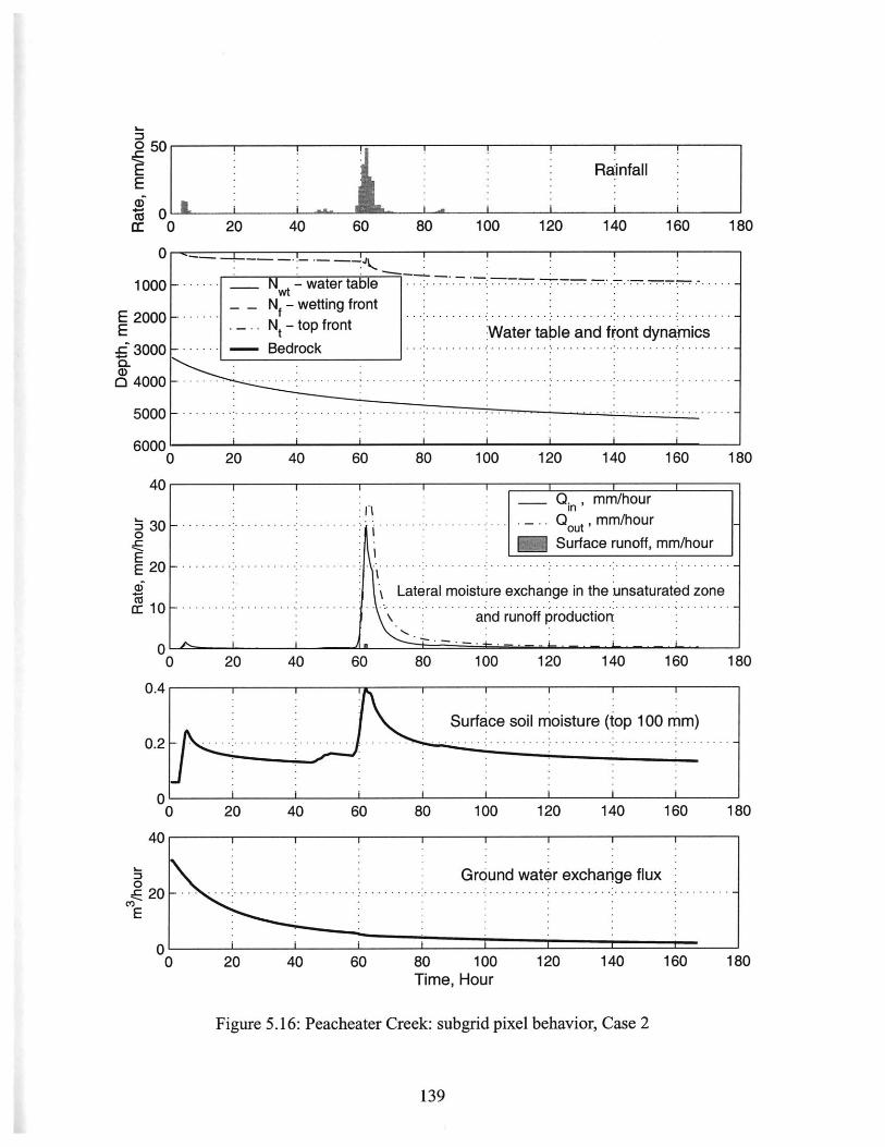
Rainfall
-
20 40 60 80 100 120
0 20 40 60 80 100 120
0 20 40 60 80 100
140 160
140
120 140
180
160 180
160 180Surface soi moisture (top 100 mm)- ......... ........ .... ....
0 20 40 60 80 100
0 20 40 60 80 100
120
120
140
140Time, Hour
Figure 5.16: Peacheater Creek: subgrid pixel behavior, Case 2
139
0
o50
E
cc
0
1000
2000
3000C-04000
5000
6000
40
3 300
EE 20
m 10
A
- - N - water table -
N - wetting front- - top front- t Water table and front dynamics
---.. - Bedrock - - - - - - - - - - - --
.- .
- . . .. ..-. . . . . .--.- -. ..- -.-. .- -
Q ,mm/hour- --- - - outmm/hour
Surface runoff, mm/hour
Lateral moisture exchange in the unsaturated zone
and runoff production
0.4
0.2
0
4U
Ground water exchange flux
160 1E
160 1E
0
0

Rainfall
20 40 60 80 100
0 20 40 60 80 100
20 F
15 ................Lateral
120
120
140
140
160 180
160
o50
E
4-0ca 0
0
1000
2000
3000
4000
5000
6000
Q, mm/hour-..-. out , mm/hour
Surface runoff, mm/hour
moisture exchange in the unsaturated zone
and runoff production
0 20 40 60 80 100 120 140 160
0 20 40 60 80 100
150
100
50
0 20 40 60 80 100 120 140Time, Hour
Figure 5.17: Peacheater Creek: subgrid pixel behavior, Case 3
140
0)
180
Water table and front dynamics N - water table-.. ..... -......... -. - -.-.-.-.-..-.-.-.- - Nf - w etting front
N - top front- - - -- -- ---- . . .- .- . . . -... ..- ..... t .Bedrock
-.-.-.- - -.- - - - -.-
0.4
0.2
0
Surface soil moisture (top 100 mm)......................... .....................................
180
120 140 160 180
. . .. . . . . . . . . . . . . . . . . . . . . . . . . . . . . . . .I .. . . . . . . . . .
Ground water exchange flux- - . .
160 180
N

CHAPTER VI
Conclusions
6.1 Summary of development and implementation results
The work discussed in the previous chapters presents enhancements to a hydrologic simula-
tion package RIBS, the Real-Time Interactive Basin Simulator (Garrote, 1993). The RIBS
model was developed as a rainfall-runoff event-based model that accounted for the effects
of slope and soil vertical and horizontal heterogeneity through a simplified formulation of
the infiltration process and lateral exchange in the unsaturated zone. It offers an integrated
software package allowing for distributed raster-based hydrologic simulation within a
graphical environment. The model has been tested for a number of watersheds in Italy and
the continental U.S.
The modifications made in the existing model framework, in terms of description of
infiltration and subsurface saturated lateral exchange processes, significantly enhance simu-
lation capabilities of the model. The major changes concern:
- Development and implementation of a modified Green-Ampt scheme which can be
applied for soils that exhibit exponential decay of the saturated conductivity with
depth. Introduction of this parameterization allows for accounting of capillary
effects during the infiltration process, for both the unsaturated and saturated phases.
- Development and implementation of a soil moisture redistribution scheme that pro-
vides a physically sound way to mimic the dynamics of the soil moisture profile dur-
ing rainfall hiatus and interstorm periods.
- Implementation of a parameterization that allows one to simulate evaporation condi-
tions and hence extract moisture from a soil water profile. This procedure is used
when simulating interstorm conditions. This significantly expands the range of
meteorological conditions under which the model can be used.
141

- Development and implementation of a scheme allowing for simulation of the process
of lateral moisture transfer in the ground water system. A simplified procedure
accounts for the soil heterogeneity and decay of the saturated conductivity with
depth. This permits modeling of the ground water dynamics using the Dupuit
assumptions for phreatic aquifer saturated flow.
- Development and implementation of an unsaturated - saturated zone coupling
scheme which is important for simulation of the interaction between moving fronts
and changing ground water level. This coupling scheme ensures the model's appli-
cation for long periods of time, a necessary condition for the continuous rainfall-
runoff simulations.
Overall, the model modifications enhance the range of potential RIBS applications.
The most important changes include the capability of simulating catchment hydrologic
response continuously, i.e. during storm, storm hiatus, and inter-storm periods. For the
description of principal hydrologic processes the model uses simplified parameterizations
that result in higher computational efficiency with respect to the numerical solution of the
governing differential equations. The hydrologic simulation package is implemented as a
flexible module in C++ and can be easily integrated with another type of distributed hydro-
logic model.
Another important aspect of the presented work is estimation of the basin state at the
beginning of the storm. A new soil moisture initialization scheme has been implemented
which is different from the kinematic parameterization used in the original RIBS version
(Cabral et al., 1992). This made it possible to resolve problems with the estimation of the
decay parameter,f, of hydraulic conductivity. The soil moisture profile is inherently tied to
the water table depth, and thus the initial location of the ground water level defines the
catchment wetness conditions. An independent routine has been developed that obtains the
spatial distribution of the depth to the water table in a basin. Based on a steady state
assumption of the topography controlled groundwater (Sivapalan et al., 1987), the approach
142
consistently simulates a wetter initial state in the convergent areas and dryer initial condi-
tions in the divergent areas. A series of initial ground water level distributions can be pro-
duced for the calibration procedure. At the same time, the capability of continuous
simulation allows for smoothing of the effects of errors in catchment initialization.
6.2 Summary of simulation results
The current work presents two basic types of simulations: off-line modeling of a
pixel that does not involve using the full hydrologic package and representation of a hills-
lope or basin using the complete RIBS software environment.
The purpose of the off-line simulations is to demonstrate the physical validity of the
assumptions and to test each of the model processes in an independent framework. Several
infiltration tests have been presented to illustrate the sub-grid pixel behavior corresponding
to ponded infiltration, and infiltration under conditions of rainfall with constant and variable
intensity. The latter example also included simulation of an interstorm period. The concep-
tual validity of the formulation has been demonstrated for a typical loamy soil. The evalua-
tion of how the infiltration parameterizations compare with the numerical solution of the
Richard's equations or laboratory infiltration experiments is not performed in this thesis and
can be suggested as a future research effort.
Another off-line test involve modeling the ground water flow for different partition-
ing schemes considered by the model. A comparison with the two 2-D analytical solutions
of a linearized form of the Boussinesq's equation has been conducted. The model perfor-
mance was good and the ground water flow partitioning scheme was shown to be generally
valid.
The complete system simulations were performed for two different cases: an artifi-
cial hillslope model and a natural watershed. The first simulation is used to demonstrate the
model's capability to simulate the principal phases of hydrologic response of a system that
couples the unsaturated zone and ground water. As long as the hillslope topography has a
1-D structure, it is a good example for showing how realistically the model simulates the
143

lateral interaction between the computational elements. As it has been demonstrated, the
model is capable of continuously simulating the principal phases of meteorologic forcing in
both the unsaturated and saturated zones.
A calibration test for Peacheater Creek provides a good example of what the model
is capable of accomplishing when properly applied. Using real storm rainfall data, the fit of
the model output to the actual storm flow is found to be reasonably good. The calibrated
parameter values are within the physically reliable ranges. The hydrograph partitioning
according to the runoff types is consistent with an apriori reasoning.
Overall, the presented simulation results are physically sound and encouraging. The
scope of model applications was limited to several cases and should be expanded in the
future to include simulation of basin hydrologic response to a sequence of storm events over
extended periods of time, as well as calibration and verification tests for other watersheds.
144

APPENDIX 1
The Green-Ampt model for non-uniform soils.Formulation of the wetting front capillary drive.
The Green and Ampt [1911] model of infiltration has been the subject of considerable atten-
tion in the hydrological literature. The standard Green-Ampt model follows from assuming
that for the moisture front infiltrating into a semi-infinite, uniform (homogeneous) soil at
uniform initial volumetric water (O, = const) content, there exists a precisely defined wetting
front for which a water pressure head hf remains constant with time and position. Behind
the wetting front, the soil is uniformly saturated with a constant conductivity K, correspond-
ing to a natural saturation. The movement of water in the soil is assumed to be in the form
of a discontinuous piston-like front. For the ponding condition the potential at the surface is
equal to the depth of the ponded water ho. Under the above assumptions the Green-Ampt
model can be expressed as:
qn = -KS (hfh Nf) (A1.1)Nf
where Nf is depth of the wetting front. The Green-Ampt model represents a limiting case
when the diffusivity increases rapidly with the water content, i.e. approaches the delta func-
tion (Philip [1969]). Though the Green-Ampt equation is a simplified representation of the
infiltration process in the field, there have been a number of demonstrations of applicability
of the formula and the good agreement with data.
The Green-Ampt formulation assumes that the soil has a vertically uniform hydrau-
lic conductivity. Furthermore, it assumes a uniform initial moisture content as the anteced-
ent condition. The following modifications of the Green-Ampt formulation allow for non-
uniform moisture distribution and non-uniform saturated hydraulic conductivity.
As in the classical Green-Ampt model, let's consider a soil of semi-infinite vertical
extent. The soil is assumed to be vertically non-uniform and has an initial soil moisture
145

variation with depth 0, = Of n). At time t = 0 the soil surface is flooded with water of depth
ho and infinite lateral extent. Keeping the level of the pond constant, water will infiltrate
into the soil at a rate that is completely determined by the soil characteristics, the initial
pressure head, and the depth of ponding. The one-dimensional Darcy's law for the vertical
flux at any point of the wetted profile is:
qn = -K() - K(6) - D(O) (A 1.2)
where is the capillary potential gradient and D(0, n) is the soil's diffusivity. Thean
Green-Ampt concept of piston displacement implies that the vertical flux may change with
time but not with depth. This implies that the flux is assumed to be constant over the whole
saturated thickness at any instantaneous time. The assumption is especially strong for verti-
cally non-uniform soils. In vertically non-uniform soils the pressure distribution within the
saturated profile has to be considered. Since the elevation gradient is constant and the satu-
rated hydraulic conductivity decreases with depth, constant normal flow within the satu-
rated zone implies a positive pressure buildup. Pressure gradients compensate for the decay
of conductivity in successive layers to keep the flux constant. Assuming lateral effects are
negligible (infinite soil extent):
aq~= 0 (A1.3)an
and thus:
K e' - = 0 (A 1.4)
This yields a differential equation governing the pressure distribution within the saturated
profile:
2
- f +f = 0 (A1.5)an 2 an
146
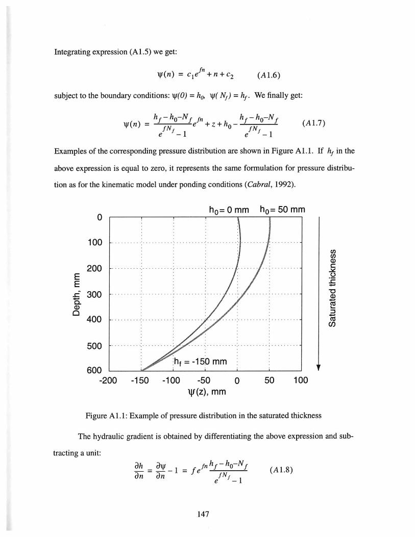
Integrating expression (Al.5) we get:
g(n) = ce fn+n+c2 (A1.6)
subject to the boundary conditions: xV(O) = ho, i( N) = hf. We finally get:
= hf - ho-Nf fn hf - ho-NffNf e +z+h 0 - fNf
e - I
(A 1.7)
e -1
Examples of the corresponding pressure distribution are shown in Figure Al.1. If hf in the
above expression is equal to zero, it represents the same formulation for pressure distribu-
tion as for the kinematic model under ponding conditions (Cabral, 1992).
0
100
200
300
400
500 . ..
hf = -150600
-200 -150 -100 -50 0 50lW(z), mm
Figure A1.1: Example of pressure distribution in the saturated thickness
The hydraulic gradient is obtained by differentiating the above expression and sub-
tracting a unit:
Ah = _
an anf n h O-Nf
=fe fNfe --(A1.8)
147
100

and the Darcian flux at any point of the saturated thickness is therefore given as:
qn(n) = -KOne 1 = -K0n [hf-hel] (A1.9)q -K ~e - 1 (A19
The equation can be expressed in a more generalized way:
h f-hoqn(Nf) = -Keff IN 0h-1] (A1.10)
where Keg is the harmonic mean of the conductivities over the saturated depth:
Nf
f dnKf(Nf) = Nf0 (A1.11)
SdnK (n)
sn0
The expression (A1.10) is a modified version of the Green-Ampt model for non-uni-
form soil where Keff and hf are monotonically decaying functions of depth N. One can see
that asf approaches zero, equation (A1.10) becomes the classic Green-Ampt formulation
for homogeneous soil (equation (A1.1)). The same expression was obtained by Beven
[1984] as a generalization of the relationship for the infiltration rate for a layered soil given
by Childs and Bybordi [1969]. The formulation has proven to adequately model the experi-
mental data of Childs and Bybordi [1969].
It is necessary to note that the capillary pressure hf used as the boundary condition
above is not a precisely defined value. Figure A1.2 depicts a general profile of soil moisture
(solid line) under ponding conditions. It also shows the Green-Ampt soil moisture profile
modeled in abrupt step-wise manner at n = Nf (dashed line). At the trailing edge of the
wetting front (or depth No ) of the general soil moisture profile, the capillary suction is
close to the saturated value, or zero. For the remainder of the wetted edge No < n < N , it
is less than zero and equals to some value between zero and that corresponding to the initial
soil moisture Q,(Nn ) at the depth Np n. This value is much lower than the modeled hf at the
148

depth Nf. Hence in the formulation above, hf represents an average capillary suction at
the wetting front modeled as a piston. The discussion follows.
Oi(n) OS,r- e
n ' "
Figure A1.2: A sketch of the general and the Green-Ampt soil moisture profiles
There has been long discussion in the literature over the proper assignment of hf in
the Green-Ampt model. It has been interpreted in various ways. Bouwer [1964] was the
first researcher who suggested that hf be linked to measurable soil characteristics:
hf = IJK(W) dy = - 1D(0) d (A1.12)
where K, is the saturated hydraulic conductivity of a uniform soil. As it has been shown
(Mein and Larson, 1973, etc.), the Bouwer's formulation of the capillary drive term has
been successfully tested in a number of applications. Later it was suggested that hf to be
represented by the water entry pressure head which is a half of the air entry bubbling pres-
sure (Whisler and Bouwer, 1970; Rawls et al., 1983). Morel-Seytoux and Khanji [1974]
149

came up with a similar to the Bouwer's expression taking into account the flow of air under
the wetting front. Nonetheless, the formulation did not lead to better agreement with exper-
iment (Neuman [1976]). Neuman [1976] derived the Bouwer's expression analytically and
suggested its modification for small values of time of the infiltration process. Recently,
Selker; et al. [1999] suggested an expression for soils having exponential decay of the satu-
rated conductivity with depth based on Miller's similarity theory (Miller and Miller, 1956):fn
hf(n) = hfe 2 (A 1.13)
where hfo represents either the wetting front pressure at Nf = 0 or the capillary drive for
uniform saturated conductivity (f= 0). This formulation, however, does not give any insight
on dependence of h/n) on the initial soil moisture distribution 0(n) in the soil. Such a
dependence, nevertheless, is observed and physically justified. Ambiguity in assigning hfo
is the second important factor which one has to consider when using the parameterization
(A1.13). The parameter is not related to the textural soil properties in any explicit way. An
attempt is therefore made to modify and apply formulation (Al.12) for the case of non-uni-
form soil.
As it was pointed out, hf represents an average capillary suction at the wetting front.
Physically, it must depend on the initial pressure head corresponding to the initial soil mois-
ture distribution, soil hydraulic properties, and changes of these properties with depth. Fol-
lowing derivations by Neuman [1976], and recognizing that the infiltration flux qn is
assumed to be constant with depth at any instantaneous time, expression (A1.2) in the form
containing the diffusivity term can be integrated along the wetted profile to the depth of the
wetting front Nf (ponding depth ho is assumed to be zero):
Nf Nf Os
f qdn= JK(O)dn + D(0)dA (A1.14)
0 0 0,(Nf)
150

where the moisture value at the wetting front is taken as the initial moisture value 0, . As
long as the flux is assumed to be constant:
Nf O,
qnNf= fK(0)dn+ f D(0)dA (A1.15)
0 Oi(Nf)
Invoking the assumption of constant flux at any point in the saturated thickness, we assume
that at any instantaneous time the soil essentially behaves as homogeneous with K, = Kff
(N). This also can be verified by comparing equations (A1.1) and (A1.10). For the Green-
Ampt profile 0 = 0, for 0 < n < Nf and hence K(0) = Ks for the same range of depths, and
hence the first term in the right part of the expression (A1.15) becomes:
OS
qn Nf = -Keff(Nf)Nf + f D(0)dA (A 1.16)
Oi(Nf)
Comparing the above equation with the expression obtained before for the constant flux
within the saturated zone (Al.10), it follows that the capillary drive across the wetting front
is:
Os
hf (O(Nf), Nf) = - ) D(0) dO (A 1.17)
0(Nf)
It can be seen that the obtained expression is similar to the one derived by Neuman [1976]
with the difference that the integral is weighted by Keff(N). The expression considers the
integral value of diffusivities over the moisture range corresponding to the initial moisture
value at depth Nf and moisture saturation value QS . As f approaches zero, the equation
becomes exactly (A1.12), i.e. behaves consistently in f zero limit.
151
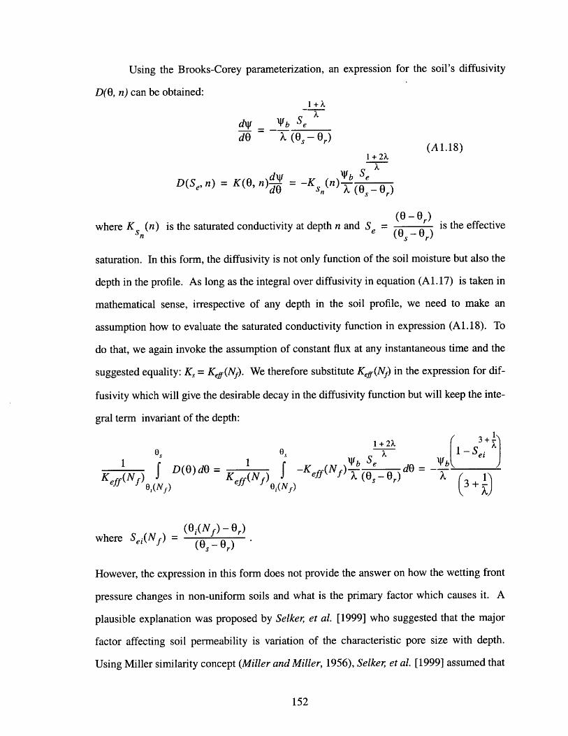
Using the Brooks-Corey parameterization, an expression for the soil's diffusivity
D(O, n) can be obtained:1+X
dW W_ b SeX
dO X(OSO 1+2X(A1.18)
dV Wb SeXD(S , n) = K(O, n) = -K b (n) s-D(e~l)=dO n, X (OS -r)
(0 -Or)where K (n) is the saturated conductivity at depth n and Se = (0 ~ Or is the effective
saturation. In this form, the diffusivity is not only function of the soil moisture but also the
depth in the profile. As long as the integral over diffusivity in equation (A1.17) is taken in
mathematical sense, irrespective of any depth in the soil profile, we need to make an
assumption how to evaluate the saturated conductivity function in expression (A1.18). To
do that, we again invoke the assumption of constant flux at any instantaneous time and the
suggested equality: Ks = Keff(N). We therefore substitute Keff(N) in the expression for dif-
fusivity which will give the desirable decay in the diffusivity function but will keep the inte-
gral term invariant of the depth:
0 0 1 + 2X1-S3+
1 1 Vb Se do b( e1D(O)d = -Keff(N) d =-
Keff (Nf)0,(Nf ) Keff(Nf)0;(N5) X (Os ~Or 3+
(0 (()Nf,.
where Sei(Nf) = (O.(Nf) - O)(OS -Or)
However, the expression in this form does not provide the answer on how the wetting front
pressure changes in non-uniform soils and what is the primary factor which causes it. A
plausible explanation was proposed by Selker et al. [1999] who suggested that the major
factor affecting soil permeability is variation of the characteristic pore size with depth.
Using Miller similarity concept (Miller and Miller, 1956), Selker et al. [1999] assumed that
152

the conductivity decay rate would be the square of the decrease rate in pore size. Indeed,
the notion is well supported by the observation that while many soils exhibit sharp decay in
the saturated conductivity with depth, variation of the total porosity is negligible (Beven,
1982, 1984). It has also been widely reported that soils show high variability in characteris-
tic particle size with depth. Selker, et al. [1999] further assumes an expression which relates
changes in conductivity with changes in pore size for soils that obey Miller scaling:
fn
X(n) = XAe 2 (A1.19)
where X0 is the characteristic pore-size distribution index of the top layer of a vertically fin-
ing soil. The expression for hf therefore becomes:
f1
3 +
hf(Nf) = X(Nf) (A 1.20)3X(Nf) + 1
It can be seen that as f -> 0 the expression will approach and never exceed Ny . This is a
reasonable result as the air entry bubbling pressure is an integral characteristic of the magni-
tude of suction potential in the soil.
Sensitivity of the capillary drive term with respect to the initial soil moisture O,
parameters f , and X0 is shown in Figure (A 1.3). As it is expected, the capillary suction in
the formulation (A1.20) exhibits rather strong dependence on the parameter f , sharply
growing with f and the depth at which it is evaluated. hf also exhibits strong dependence
on X0 , being especially noticeable for finer soils with X0 < 1. It is quite interesting to note
that hf does not show much variation with respect to the initial soil moisture for the range
0, / o, 0.5. It does quickly go to zero for values of O6 / O, > 0.5.
As a first-order validation of the formulation for the wetting front suction, a data set
of experiment by Childs and Bybordi [1969] is used. It has been previously shown (Beven,
1984; Selker et al., 1999) that the constant flux formulation (equation (A1.10)) agrees well
153

with the observations obtained in this experiment. The top plot in Figure (A1.4) shows the
fit of the exponential function to the saturated conductivity data. The higher and lower
envelopes contain all the data points and the interior dashed line, which is obtained using
average value of f= 0.0018 mm-1, is assumed to be describing the data reasonably well. As
long as for all the data points 0, / 0, 1 - 0.35 / 0,, we may neglect the Sei (Nf) term in
equation (A1.20) due to the negligible variation of hf for the initial soil moisture in the
range O6 / 0, 0.5 as noted above. We may fit the wetting front suction observed by
Childs and Bybordi [1969] using two or more of the data points. The bottom plot in Figure
(A1.4) shows examples of possible fits with estimated values of Xb and X0 . These are
shown for illustration purpose only implying that the fit is possible with physically mean-
ingful values of the parameters. The model in the form (A1.20) therefore has a potential of
predicting change in the wetting front capillary drive for vertically non-uniform soils.
154

- r
Capillary drive term h as a function of wetting front depth Nf and 8,(Nf)
-30
.e-40
-50 -- . ... . .
E............ .................. .... ... ...... .........- 10 0 -..-- -...-- -...---.. ---.. -- - - - -
- 1 5 0 -. .. .- . . . .- -. . . .-. -. .- - -.-. .--..--- -. -.. -N = 1001
Nf = 2000 mm:
-200-0 0.001 0.002 0.003 0.004 0.005 0.006 0.007 0.008
f, mm
EE
-200
0.009 0.01
1 0.5 1 1.5 2 2.5 3 3.5x0
Figure A1.3: Sensitivity of the capillary drive term to various parameters
155

Fit of Ksn(n) function to the data of Childs and Bybordi [1969]0
200
400
600
800
1000
1200
1400
1600
1800C 14000 16000 18000
Fit of hf(n) function to the data of Childs and Bybordi [1969]
O Wetting front suction, Childs & Bybordi, 1969Fit yb = -1050 mm, X = 6.29
- ~ Fit b = -5 70 mm, X = 3.25
.00.
--e
-o -
-~
- - . .
-
-.
.-0,
- - -.
- - - -.
- - - - - - - -.
- - - - -.
- - - -... ...
-220 -200 -180 -160 -140 -120hf, mm
Figure A1.4: Fit of the model to the data of Childs and Bybordi [1969]
156
2000 4000 6000 8000 10000 12000K,, mm/hour
....1...... .. . .... .. . . . .
-.-.--.- Higher envelope, f = 0.0021 mm ~
- Lower envelope, f =0.0015 mm~
- -- :--- - f=0.0018mm 1
0
200--
400-.
600-
800--
1000--
1200--
1400--
1600--
1800-240
-:-:
-100 -40-80 -60
----- -----
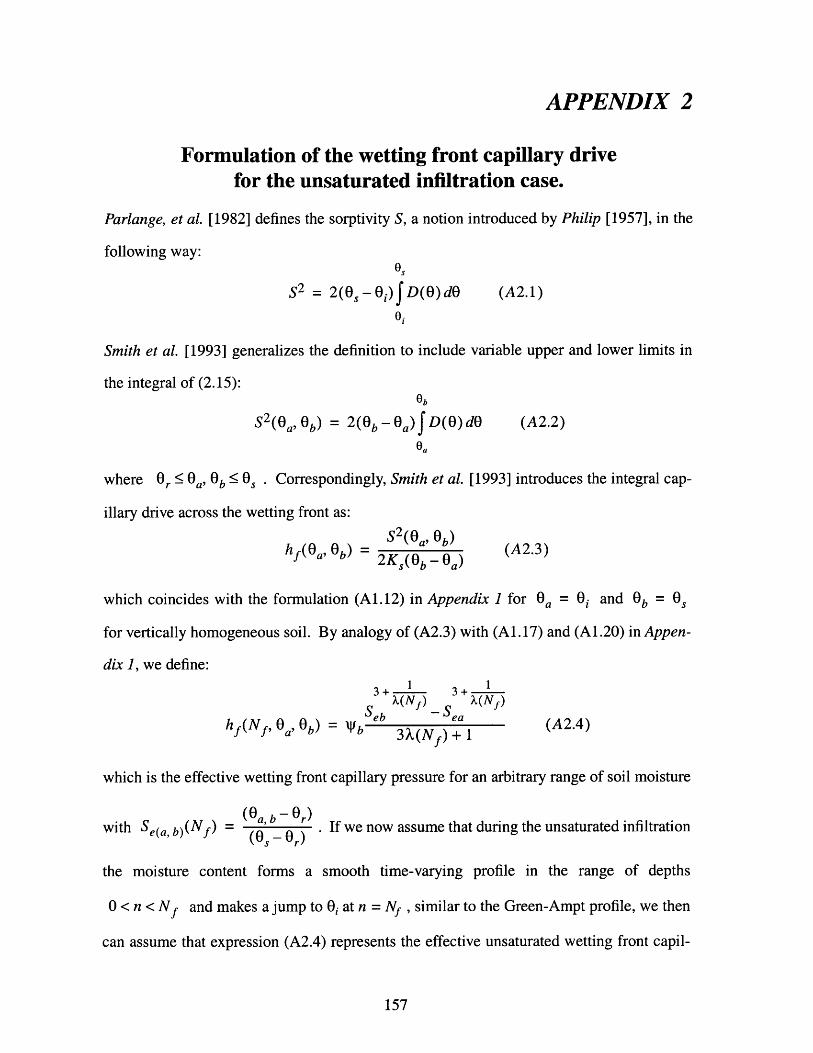
APPENDIX 2
Formulation of the wetting front capillary drivefor the unsaturated infiltration case.
Parlange, et al. [1982] defines the sorptivity S, a notion introduced by Philip [1957], in the
following way:0S
S2 = 2(O, - O) fD(O) dO (A2.1)
Si
Smith et al. [1993] generalizes the definition to include variable upper and lower limits in
the integral of (2.15):
S2(Oa, Ob) = 2(Ob - Oa) fD(O) dO (A2.2)
where 0_<0 i., Ob OS . Correspondingly, Smith et al. [1993] introduces the integral cap-
illary drive across the wetting front as:
=S2(a, Ob)2Ks(O, - 0 a)
(A2.3)
which coincides with the formulation (Al.12) in Appendix 1 for Oa = 0i and Ob = s
for vertically homogeneous soil. By analogy of (A2.3) with (A1.17) and (A1.20) in Appen-
dix 1, we define:
hf(Nf, 0 a' 0b)
e X(Nf) 3+X(Nf)b -S e
~~ b b 3X(Nf) + 1
which is the effective wetting front capillary pressure for an arbitrary range of soil moisture
with Se(a, b)(Nf) = (Oa, b - Or . If we now assume that during the unsaturated infiltration(OS - Or)
the moisture content forms a smooth time-varying profile in the range of depths
0 < n < Nf and makes a jump to O at n = Nf , similar to the Green-Ampt profile, we then
can assume that expression (A2.4) represents the effective unsaturated wetting front capil-
157
(A2.4)

lary pressure with 0a = Oi , Ob = some unsaturated moisture value corresponding to the max-
imum water content in the wetted edge.
158

APPENDIX 3
Derivation of an equation for evolution of thetop front of the perched saturated zone.
Let's consider a domain Q that is delineated by the planes p = Pi I P = P2, n = nj , n = n2,
with nj = 0 < N, < n2 < N (Figure A3.1). At any time step t, the total moisture amount con-
tained in the domain Q , MT1 , can be expressed as a sum of moisture contained between the
top front Mat and the soil surface nj = 0 and moisture Mb' contained between the top front
and depth n2 :
t p2
nN t
Nf
1.qn(N, t N )
n
Figure A3. 1: An illustration of the domain of interest L2
As long as an assumption of constant unsaturated conductivity in the profile of infiltrated
water is made, the term Mat is defined by an integration of equation (2.16), Chapter 2. The
term Mbt accounts for water contained in the saturated perched zone, and both terms are
defined by the current location of the top front Ntt :
N' I fN")
Mt = f(n)d = (Os~-r{)1-e +rN (A30 f (A3.2)0
M = Os(n2-Nt)
159
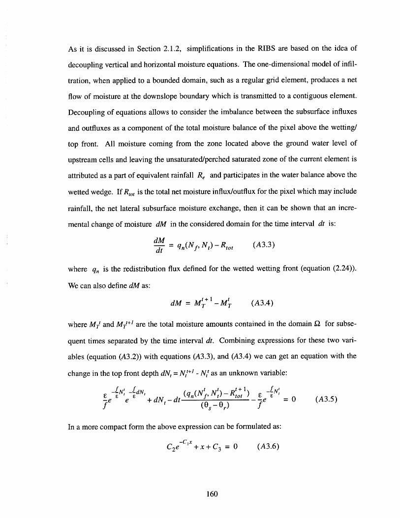
As it is discussed in Section 2.1.2, simplifications in the RIBS are based on the idea of
decoupling vertical and horizontal moisture equations. The one-dimensional model of infil-
tration, when applied to a bounded domain, such as a regular grid element, produces a net
flow of moisture at the downslope boundary which is transmitted to a contiguous element.
Decoupling of equations allows to consider the imbalance between the subsurface influxes
and outfluxes as a component of the total moisture balance of the pixel above the wetting/
top front. All moisture coming from the zone located above the ground water level of
upstream cells and leaving the unsaturated/perched saturated zone of the current element is
attributed as a part of equivalent rainfall R, and participates in the water balance above the
wetted wedge. If Ror is the total net moisture influx/outflux for the pixel which may include
rainfall, the net lateral subsurface moisture exchange, then it can be shown that an incre-
mental change of moisture dM in the considered domain for the time interval dt is:
dM= qfn(Nf, N,) - Ro, (A3.3)
where q, is the redistribution flux defined for the wetted wetting front (equation (2.24)).
We can also define dM as:
t + 1dM = MT - Mr (A3.4)
where MT and M/+1 are the total moisture amounts contained in the domain Q for subse-
quent times separated by the time interval dt. Combining expressions for these two vari-
ables (equation (A3.2)) with equations (A3.3), and (A3.4) we can get an equation with the
change in the top front depth dNt = N+l - N,' as an unknown variable:-LN -LN, (A t _Rt t + 1 LNt
E FN -, n(N, ) E -Ne e +dNt-dt ( 0 = 0 (A3.5)
f (Os - Ord
In a more compact form the above expression can be formulated as:
C2 e cjx+x+C 3 = 0 (A3.6)
160

where the coefficients are the following:
x = dN,
C1E
12-C, N (A3.7)
t - t + I(q,(Nf, N -R 1 , )t -
C3 = dt (-s-C)
The solution of equation (A3.6) is found through a Lambert W function defined as the root
of the equation: W(z)eW(z) = z . A detailed description is given by Corless et al. [1996].
The root of equation (A3.6) is:
t+1 t 1C(C-)N, - N, = -LambertW e - C (A3.8)
A new top front depth for time t+1 therefore can be obtained given its previous position Ntt
at time t, the total net moisture influx/outflux for the pixel Rto/+1 during time interval dt, and
the redistribution flux at the wetting front depth q,. The above expression holds only if the
perched saturation zone will persist for time t+1.
161

162

APPENDIX 4
Derivation of an equation for the water table depthgiven the soil moisture deficit.
If the initialization soil moisture profile in the unsaturated zone is defined as:
0(n) = Or +(Os -r) (A4.1)
where the notation of the variables follows those of Section 2.1, and 3.2, then the total
amount of moisture M, contained in the profile above the water table located at depth Nw,
is expressed as:
M= f 0(n)dn = Or(Nwt +b)0
N VbN*';V- N bos
(X0o-1) +
The moisture deficit dM, the water depth required to saturate the soil, can therefore be
expressed:
dM = OsN, -M, =
= 0/(Nw + Vb) - Or(Nwt+ b)(Os - r) [(X 0- 1) b
b t }+N_,+ N ,V
Following from expression (A4.3), the knowledge of the moisture deficit allows to compute
the depth to the water table Nwt as a root of the following equation:
C1N +CN, -I +C 2 = 0
where C1 , C2 , and C3 are the constants that are equal to:
C1 = Os -Or
C1 (-Wb(X 0- 1)
CX1)-(o - 1)
(A4.4)
(A4.5)
+ Cltb -dM
163
(A4.2)
(A4.3)

As long as the value of X0 is generally not an integer value, equation (A4.4) is solved using
the Newton iteration procedure for root finding (Press, et al., 1999).
164
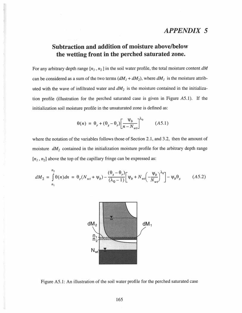
APPENDIX 5
Subtraction and addition of moisture above/belowthe wetting front in the perched saturated zone.
For any arbitrary depth range [nj, n2 ] in the soil water profile, the total moisture content dM
can be considered as a sum of the two terms (dM + dM2), where dM is the moisture attrib-
uted with the wave of infiltrated water and dM2 is the moisture contained in the initializa-
tion profile (illustration for the perched saturated case is given in Figure A5.1). If the
initialization soil moisture profile in the unsaturated zone is defined as:
0(n) = Or +(Os - Or)[" - Nb(A5.1)
where the notation of the variables follows those of Section 2.1, and 3.2, then the amount of
moisture dM2 contained in the initialization moisture profile for the arbitrary depth range
[n1 , n2] above the top of the capillary fringe can be expressed as:
dM 2 = 0(n)dn = Or(N,,t+Vb- s - r7+N,,_- - Wb0S
dM 2
ni.n2-
NW
(A5.2)
dM 1
Figure A5.1: An illustration of the soil water profile for the perched saturated case
165

In the perched saturated case, the moisture content dM is equal to 0, (n2 - n1 ) = dM + dM2 -
This relationship can be used to find one of the depths (n2 or nj) if the amount of moisture
dMI contained in the wave of infiltrated water is known. Combining this relationship with
expression (A5.2) one can obtain:
CI(n l - n2)+ C 2 -- 1 I + dMi = 0 (A5.3)
.(Nt,-n2) 0 (N,,-n )
where the coefficients C, and C2 are:
C1 = ( s - GO)
(~vb)Xo (A5.4)
2 1(X0 _ 1)
If n2 is the known wetting front depth and dM is the moisture content which is required to
be extracted out of the perched zone, then equation (A5.3) must be solved for nj (smaller
than n2 )- If nj is the known wetting front depth and dM is the moisture content which is to
be added to the perched zone, then equation (A5.3) must be solved for n2 (larger than nj ).
As long as the power X0 is generally not an integer value, then equation (A5.3) can not be
solved in either case in a closed form. A numerical scheme, the Newton iteration procedure
for root finding, is used to find the depth of interest (Press, et al., 1999).
166

Bibliography
Abbott, M.B., J.C. Bathurst, J.A. Cunge, P.E. O'Connell, and J. Rasmussen, An introduction tothe European Hydrological System - Systeme Hydrologique European,'SHE', 1: History andphilosophy of a physically-based distributed modelling system, J. of Hydrology, 87, 45-59,1986a.
Abbott, M.B., J.C. Bathurst, J.A. Cunge, P.E. O'Connell, and J. Rasmussen, An introduction tothe European Hydrological System - Systeme Hydrologique Europeen 'SHE', 2: Structure of aphysically based, distributed modelling system, J. of Hydrology, 87: 61-77, 1986b.
Abbot, M.B. and J.C. Refsgaard, Distributed hydrologic modeling, Kluwer Academic Publishers,1996.
Anderson, M.G. and T.P. Burt as editors, Process studies in hillslope hydrology, Chichester, WestSussex, England; New York, Wiley, 1990.
Bear, J., Dynamics of fluids in porous media, American Elsevier Pub. Co., Environmental Series,New York, 1972.
Bear, J., Hydraulics of groundwater, McGraw-Hill Series in Water Resources and EnvironmentalEngineering, 1979.
Berger, K.P., Surface ground-water interaction: the spatial organization of hydrologic processesover complex terrain, Ph.D. thesis, Civil and Environmental Engineering Dept., MIT, 2000.
Beven, K.J., On subsurface stormflow: predictions with simple kinematic theory for saturated andunsaturated flows., Water Resour Res., 18(6), 1627-1633, 1982b.
Beven, K.J., On subsurface stormflow: an analysis of response times, Hydr Sci. J., 27(4), 505-521, 1982b.
Beven, K.J., Infiltration into a class of vertically non-uniform soils, Hydr Sci. J., 29(4), 425-434,1984.
Beven, K., Calver, A. and Morris, E. M., Institute of hydrology distributed model, InternalReport, Institute of Hydrology, Wallingford, 1987.
Bouwer, H., Infiltration of water into nonuniform soil, J. Irrig. Drain. Div. Amer Soc. Civ. Eng.,95 (IR4), 451-462, 1969.
Bouwer, H., Unsaturated flow in ground water hydraulics, J. Hydraul. Div. Amer Soc. Civ. Eng.,90 (HY5), 121, 1964.
Bras, R.L., Hydrology. An introduction to hydrologic science, Addison-Wesley, 1990.
Broadbridge, P., and I. White, Constant rate rainfall infiltration: a versatile nonlinear model, 1,Analytic solution, Water Resour Res., 24(1), 145-154, 1988.
Brooks, R.H., and A.T. Corey, Hydraulic properties of porous media, Hydrol. Pap. 3, 27pp, Colo.State Univ., Fort Collins, 1964
167

Brutsaert, W., and J.L. Nieber, Regionolized drought flow hydrographs from a mature glaciatedplateau, Water Resour Res., 13(3), 637-643, 1977.
Cabral, M.C., L. Garrote, R.L. Bras, and D. Entekhabi, A kinematic model of infiltration and run-off generation in layered and sloping soils, Adv. in Water Resources, 15, 311-324, 1992.
Carslaw, H.S., and J.C. Jaeger, Conduction of heat in soilds, 2nd edition, Oxford University Press,London, 1959.
Charbeneau, R.J. and R.G. Asgian, Simulation of the transient soil water profile for a homoge-neous bare soil, Water Resour Res., 27(6), 1271-1279, 1991.
Coles, N.A., M. Sivapalan, J.E. Larsen, P.E. Linnet, and C.K. Fahrner, Modeling runoff genera-tion in small agricultural catchments: can real world runoff responses be captured?, Hydrologi-cal processes, 11, 111-136, 1997.
Corless, R.M., G.H. Gonnet, D.E.G. Hare, D.J. Jeffrey, D.E. Knuth, On the Lamert W function,Adv. Comput. Math, 5, 329-359, 1996
Corradini, C., F. Melone, R.E. Smith, Modeling local infiltration for a two-layered soil undercomplex rainfall patterns, J. of Hydrology, 237: 58-73, 2000.
Costa-Cabral, M., and S.J. Burges, Digital elevation model networks (DEMON): A model of flowover hillslopes for computation of contributing and dispersal areas, Water Resour Res., 30(6),1681-1692, 1994.
DeBarry, P.A. ... [et al.], technical reviewers Arnold J. ... [et al.] Geographic information systemsmodules and distributed models of the watershed: a report from the ASCE Task Committee onGIS modules and Dostributed Models of the Watershed, 1999.
Eagleson, P.S., Climate, Soil, and Vegetation, Water Resour Res., 14(5), 706-775, 1978.
Entekhabi, D., Personal communication, 1999
Fairfield, J., and Leymarie, Drainage networks from grid digital elevation models, Water ResourRes., 27(5), 709-717, 1991. (Correction, Water Resour Res., 27(10), 2809, 1991).
Famiglietti, J.S., and E.F. Wood, Evapotranspiration and runoff from large land areas, in LandSurface-Atmosphere INteraction: Observations, Models and Analysis, pp. 179-204, KluwerAcademic, Norwell Mass, 1991
Fan, Y. and R.L. Bras, Analytical solutions to hillslope subsurface storm flow and saturation over-land flow, Water Resour Res., 34(4), 921-927, 1998.
Farr, T.G., M. Kobrick, Shuttle radar topography mission produces a wealth of data, EOS, Nov.28, 2000.
Freeze, R.A., Role of subsurface flow in generating surface runoff, 2, Upstream source areas,Water Resour Res., 8(5), 1272-1283, 1972.
Freeze, R.A. and R.L. Harlan, Blueprint for a physically-based digitally simulated hydrologicresponse model, J. of Hydrology, 9, 237-258, 1969.
168

Fulton, R.A., J.P. Breidenbach, D.J. Seo, D.A. Miller, and T. O'Bannon, The WSR-88D RainfallAlgorithm, Weather and Forecasting, 13, 377-395, 1998.
Ganguly, A., Personal communication, 2000.
Gardner, W.R., Some steady state solutions of the unsaturated moisture flow equation with appli-cation to evaporation from a water table, Soil Sci., 85(5), 228-232, 1958.
Garrote, L., Real-time modeling of river basin response using radar-generated rainfal maps and adistributed hydrologic database, M.S. Thesis, R.M. Parsons Laboratory for Water Resources andHydrodynamics, MIT, 1993.
Garrote, L., R.L. Bras, A distributed model for real-time flood forecasting using digital elevationmodels, J. of Hydrology, 167: 279-306, 1995a.
Garrote, L., R.L. Bras, An integrated software environment for real-time use of a distributedhydrologic model, J. of Hydrology, 167: 307-326, 1995b.
Garrote, L. and I. Becchi, Object-oriented software for distributed rainfall-runoff models, J. ofComputing in Civil Engineering, 11(3): 190-194, 1997.
Germann, P.F., K. Beven, Macropores and water flow in Soils, Water Resour Res., 18(5), 1311-1325, 1982.
Grayson, R.B., G. Bloschl, and I.D. Moore, Distributed parameter hydrologic modelling usingvector elevation data: THALES and TAPES-C, in V.P. Singh editor, Computer models of water-shed hydrology, Water Resources Publications, 669-696, Highlands Ranch, CO, 1995.
Green, W.H. and G.A. Ampt, Studies in soil physics, J. Agric. Sci., 4, 1-24, 1911.
Johanson, R.C., J.C. Imhoff, and H.H. Davis, User's manual for the Hydrologic Simulation pro-gram - Fortran (HSPF), Technical Report EPA-600/9-80-105, U.S.A. EPA EnvironmmentalResearch Lab, Athens, GA, 1980.
Julien, P.Y. and B. Saghafian, CASC2D user's manual, Technical report, Dept. of Civil Eng., Col-orado State University, Fort Collins, CO, 1991.
Julien, P.Y. and B. Saghafian and F.L. Ogden, Raster-based hydrologic modeling of spatially-var-ied surface runoff, Water Resour Bull., 31(3), 523--536, 1995.
Kim, C.P., G.D. Salvucci, and D. Entekhabi, Groundwater-surface interaction and the climaticspatial patterns of hillslope hydrological response, Hydrology and Earth System Sciences, 3(3),375-384, 1999.
Kirkby, M. J., Hillslope hydrology, Ser.: Landscape systems, Chichester, New York , Wiley, 1978.
Klazura, G.E. and D.A. Imy, A description of the initial set of analysis products available from theNEXRAD WSR-88D system, Bulletin of the American Meteorological Society, 74(7), 1293-1311, 1993.
Kuchment, L.S., V.N. Demidov, Yu.G. Motovilov, River Runoff Formation (Physically-BasedModels), Nauka, Moscow (in Russian), 215 p., 1983.
169

Larsen, J.E., M.K. Sivapalan, N.A. Coles, and P.E. Linnet, Similarity analysis of runoff generationprocesses in real-world catchments, Water Resour Res., 30(6), 1641-1652, 1994.
Lea, N.L., An aspect driven kinematic routing algorithm, in Overland Flow: Hydraulics and Ero-sion Mechanics, edited by A.J. Parsons and A.D. Abrahams, Chapman and Hall, New York,1992.
Mein, R.G., and C.L. Larson, Modeling infiltration during a steady rain, Water Resour Res., 9(2),384-394, 1973.
Miller, E.E., and R.D. Miller, Physical Theory for Capillary Flow Phenomena, J. of Appl. Phys.,27(4), 1956.
Moore, I.D., and R.B. Grayson, Terrain-based catchment partitioning and runoff prediction usingvector vector elevation data, Water Resour Res., 27(6), 1177-1191, 1991.
Morel-Seytoux, H.J., and J. Khanji, Derivation of an equation of infiltration, Water Resour Res.,10(4), 795-800, 1974.
Neuman, S.P., Wetting front pressure head in the infiltration model of Green and Ampt, WaterResour Res., 12(3), 564-565, 1976.
O'Callaghanl, J.F., and D.M. Mark, The extraction of drainage networks from digital elevationdata, Comput. Vision Graphics Image Process., 28, 323-344, 1984.
Ogden, F.L., CASC2D reference manual, Technical report, Dept. of Civil Eng., University ofConnecticut, Storrs, CT, 1997.
Ogden, F.L., and B. Saghafian, Green and Ampt infiltration with redistribution, J. of Irrig. andDrain. Engrg., 123(5), 386-393, 1997.
Olson, D.A., N.W. Junker, and B. Korty, Evaluation of 33 years of quantitative precipitation fore-casting at the NMC, Weather Forecasting, 10. 498-511, 1995.
Parlange, J.-Y., Theory of water movement in soils: 8, one-dimensional infiltration with constantflux at the surface, Soil Sci., 114, 1-4, 1971
Parlange, J.-Y., I. Lisle, R.D. Braddick, and R.E. Smith, The three-parameter infiltration equation,Soil Sci., 133(6), 337-341, 1982.
Philip, J.R., Theory of infiltration: Parts 1-5, Soil Sci., 83-84, 1957.
Philip, J.R., Hillslope infiltration: planar slopes, Water Resour Res., 27(1), 109-117, 1991a.
Philip, J.R., Hillslope infiltration: divergent and convergent slopes, Water Resour Res., 27(6),1035-1040, 1991b.
Philip, J.R., Infiltration and downslope unsaturated flows in concave and convex topographies,Water Resour Res., 27(6), 1041-1048, 1991c.
Polubarionova-Kochina, P.Ya, Theory of Ground Water Movement (in Russian), Gostekhizdat,Moscow, 1952, English transl., by R.J.M. de Wiest, Princeton University Press, Princeton, N.J.,1962.
170

Press, W.H., S.A. Teukolsky, W.T. Vetterling, B.P. Flannery, Numerical Recipes in C, The art ofscientific computing, Sec. Ed., Cambridge University Press, 1999.
Rybarczyk, S.M., Formulation and testing of a distributed triangular irregular network rainfall/runoff model, M.S. thesis, Ralph M. Parsons Lab., Department of Civil and Environmental Engi-neering, MIT, 2000.
Quinn, P., K. Beven, P. Chevalier, 0. Planchon, The prediction of hillslope flow paths for distrib-uted hydrological modeling using digital terrain models, Hydrological Processes, 5, 59-79,1991.
Salvucci, G.D., An approximate solution for steady vertical flux of moisture through an unsatur-ated homogeneous soil, Water Resour Res., 29(11), 3749-3753, 1993.
Salvucci, G.D., and D. Entekhabi, Equivalent steady soil moisture profile and the time compres-sion approximation in water balance modeling, Water Resour Res., 30(10), 2737-2749, 1994.
Salvucci, G.D., and D. Entekhabi, Hillslope and climatic controls on hydrologic fluxes, WaterResour Res., 31(7), 1725-1739, 1995.
Salvucci, G.D., and D. Entekhabi, Ponded infiltration into soils bounded by a water table, WaterResour Res., 31(11), 2751-2759, 1995.
Senarath, S.U.S., F.L. Ogden, C.W. Downer, and H.O. Sharif, On the calibration and verificationof two-dimensional, distributed, Hortonian, continuous watershed models, Water Resour Res.,36(6): 1495-1510, 2000.
Shen, H.W., Modeling of Rivers, Edited by H.W. Shen, John Wiley & Sons, 1979.
Singh, V.P., Watershed Modeling, in V.P. Singh editor, Computer models of watershed hydrology,Water Resources Publications, Highlands Ranch, CO, 1995.
Singh, V.P., Hydrologic Systems, Volume II, Watershed Modeling, Prentice Hall, EnglewoodCliffs, New Jersey, 1989.
Sivapalan, M.K., E.F. Wood., and K.J. Beven, On hydrologic similarity, 2, a scaled model ofstorm runoff production, Water Resour Res., 23(12), 2266-2278, 1987.
Skaags, R.W. and R. Khaleel, Infiltration part of hydrologic modeling of small watersheds, C.T.Haan, H.P. Johnson, and D.L. Brakenskiek (eds.), American Society of Agricultural Engineers,1982.
Smith, R.E., C. Corradini, and F. Melone, Modeling infiltration for multistorm runoff events,Water Resources Research, 29(1), 133-144, 1993
Smith, R.E., and J.-Y. Parlange, A parameter efficient hydrologic infiltration model, Water ResourRes., 14(3), 533-538, 1978.
Smith, R.E., and R.H.B. Hebbert Mathematical simulation of interdependent surface and subsur-face hydrologic processes, Water Resour Res., 19(4), 987-1001, 1983.
Tarboton, D., A new method for the determination of flow directions and upslope areas in griddigital elevation models, Water Resour Res., 33(2), 309-319, 1997.
171
-I

Troch, P.A., F.P. de Troch, and W. Brutsaert, Effective water table depth to describe initial condi-tions prior to storm rainfall in humid regions, Water Resour Res., 29(2), 427-434, 1993b.
Troch, P.A., M. Mancini, C. Paniconi, and E.F. Wood, Evaluation of a distributed catchment scalewater balance model, Water Resour Res., 29(6), 1805-1817, 1993a.
Warrick, A.W., Application of scaling to the characterization of spatial variability in soils, Scalingin Soil Physics: Principles and Applications, SSSA Special Publication no. 25, 1990.
Warrick, A.W., D.O. Lomen, and A. Islas, An analytical solution to Richard's equation for adraining soil profile, Water Resour Res., 26(2), 263-258, 1990.
White I., and P. Broadbridge, Constant rate rainfall infiltration: a versatile nonlinear model, 2,Application of solutions, Water Resour Res., 24(1), 155-162, 1988.
Wigmosta, M.S., W.V. Lance, and D.P. Lettenmaier, A distributed hydrology-vegetation modelfor complex terrain, Water Resour Res., 30(6), 1665-1679, 1994.
Wigmosta, M.S., and D.P. Lettenmaier, A comparison of simplified methods for routing topo-graphically driven subsurface flow, Water Resour Res., 35(1), 255-264, 1999.
van Genuchten, M.Th., A closed-form equation for predicting the hydraulic conductivity of unsat-urated soils, Soil Sci. Soc. Am. J., 44, 892-898, 1980
Yeh, T.-C.J., One-dimensional steady-state infiltration in heterogeneous soils, Water Resour Res.,25(10), 2149-2158, 1989.
Zaslavsky, D., and G. Sinai, Surface hydrology: III - causes of lateral flow, J. of the HydraulicsDivision, ASCE, 107, HY1, 17-35, 1981a.
Zaslavsky, D., and G. Sinai, Surface hydrology: IV - flow in sloping layered soil, J. of the Hydrau-lics Division, ASCE, 107 (HY1), 53-64, 1981b.
Zaslavsky, D., and G. Sinai, Surface hydrology: V - in-surface transient flow, J. of the HydraulicsDivision, ASCE, 107 (HY1), 65-93, 1981c.
Zecharias, Y.B., and W. Brutsaert, The influence of basin morphology on groundwater outflow,
Water Resour Res., 24(10), 1645-1650, 1988(1).
Zecharias, Y.B., and W. Brutsaert, Recession characteristics of groundwater outflow and base flowfrom mountainous watersheds, Water Resour Res., 24(10), 1651-1658, 1988(2).
172