A CONTAGIOUS MALADY? OPEN ECONOMY

DIMENSIONS OF SECULAR STAGNATION

Gauti B. Eggertsson, Neil R. MehrotraSanjay Singh, and Lawrence Summers

Brown University

European CommissionNovember 23, 2015

1 / 27

LOW GLOBAL INTEREST RATES

NOMINAL SHORT-TERM AND LONG-TERM RATES, 1990-2015

-­‐2.0  

0.0  

2.0  

4.0  

6.0  

8.0  

10.0  

12.0  

14.0  

16.0  

Mar-­‐90  

Jul-­‐9

1  

Nov-­‐92  

Mar-­‐94  

Jul-­‐9

5  

Nov-­‐96  

Mar-­‐98  

Jul-­‐9

9  

Nov-­‐00  

Mar-­‐02  

Jul-­‐0

3  

Nov-­‐04  

Mar-­‐06  

Jul-­‐0

7  

Nov-­‐08  

Mar-­‐10  

Jul-­‐1

1  

Nov-­‐12  

Mar-­‐14  

Japan   Germany  

US   UK  

Eurozone  

0.0  

2.0  

4.0  

6.0  

8.0  

10.0  

12.0  

14.0  

Mar-­‐90  

Jul-­‐9

1  

Nov-­‐92  

Mar-­‐94  

Jul-­‐9

5  

Nov-­‐96  

Mar-­‐98  

Jul-­‐9

9  

Nov-­‐00  

Mar-­‐02  

Jul-­‐0

3  

Nov-­‐04  

Mar-­‐06  

Jul-­‐0

7  

Nov-­‐08  

Mar-­‐10  

Jul-­‐1

1  

Nov-­‐12  

Mar-­‐14  

Japan   Germany  

US   UK  

Eurozone  

2 / 27

SHORTCOMINGS OF SOME EXISTING MODELSGlobal interest rates:

rss =1β− 1 > 0

I Real interest rate must be positive in steady stateI ZLB driven by temporary shocks to discount rate

Output shortfalls and low inflation:I Persistent global ZLB episodesI Fall in inflation and poor real GDP growth

Breaking Ricardian equivalence:I Role of public debtI Role of income redistribution

US, Eurozone and Japan

3 / 27

QUESTION AND APPROACH

QuestionI Does secular stagnation survive in a open economy framework?I What are the channels by which secular stagnation spreads?I What are the interactions in policy across countries?

ElementsI Two-country OLG model:

I World natural rate of interest can be negative

I Steady state with world interest rate stuck at the zero lower bound

I Permanent slump in output:I Downward nominal wage rigidity with partial adjustment

I Output gaps in steady state across countries

4 / 27

HOUSEHOLDS

Objective function:

maxCy,Cm,Co

U ={

log (Cy) + β log (Cm) + β2 log (Co)}

Budget constraints:

Cy = By

Cm = Y − (1 + r)By + Ad + Aint

Co = (1 + r)Ad + (1 + r∗)Aint

(1 + r)By ≤ D

0 ≤ Aint

5 / 27

NATURAL RATE UNDER PERFECT INTEGRATION

Asset market clearing condition:

NtByt + N∗

t By∗t = Nt−1Am

t + N∗t−1Am∗

t

Expression for global real interest rate:

1 + rWt =

1 + β

β(1 + gt)

ωt−1Dt + (1 − ωt−1)D∗t

ωt−1 (Yt − Dt−1) + (1 − ωt−1)(Y∗

t − D∗t−1)

Determinants of the real interest rate:I Tighter average (population-weighted) global collateral

constraints reduce world real interest ratesI Higher global population growth rates raises world natural rate

6 / 27

GLOBAL SAVINGS GLUT

SYMMETRIC POPULATION: ω = 1/2

Government budget constraint and fiscal rule:

Bg∗t + To∗

t + (1 + rt) IRt−1 + Tm∗t = G∗

t +(1 + r∗t−1

)Bg∗

t−1 + IRt

To∗t+1 = β (1 + r∗t )Tm∗

t

Asset market clearing (r = r∗):

Byt + By∗

t + Bgt + Bg∗

t − IRt = Adt + Ad∗

t

Interest rate (r = r∗):

1 + rt =Dt + D∗

t

Amt − Bg

t + Am∗t − Bg∗

t + IRt

7 / 27

INFLATION TARGET AND NEGATIVE NATURAL

RATES

ZLB places a bound on steady state inflation:

Π̄ ≥ 11 + r

Π̄∗ ≥ 11 + r∗

I If the natural rate of interest is negative, steady state inflationmust be positive

I No equilibrium with stable inflationI But what happens with nominal rigidities and zero inflation

target?

8 / 27

AGGREGATE SUPPLY

Output and labor demand:

Yt = Lαt

Wt

Pt= αLα−1

t

Labor supply:I Middle-generation households supply a constant level of labor L̄I Implies a constant market clearing real wage W̄ = αL̄α−1

I Implies a constant full-employment level of output: Yfe = L̄α

9 / 27

DOWNWARD NOMINAL WAGE RIGIDITY

Partial wage adjustment:

Wt = max{

W̃t, PtαL̄α−1}

where W̃t = γWt−1Π̄ + (1 − γ)PtαL̄α−1

Wage rigidity and unemployment:

I W̃t is a wage normI If real wages exceed market clearing level, employment is

rationedI Unemployment: Ut = L̄ − Lt

10 / 27

AGGREGATE SUPPLY RELATION

0.80  

0.85  

0.90  

0.95  

1.00  

1.05  

1.10  

1.15  

1.20  

0.80   0.85   0.90   0.95   1.00   1.05   1.10  

Output  

Gross  Infla5o

n  Ra

te  

Aggregate  Supply  

11 / 27

MONETARY POLICYInflation targeting:

Πt = Π̄ if i > 0

Π∗t = Π̄∗ if i∗ > 0

Above the ZLB:I If rt > Π̄−1, nominal rate equals the natural rate

I Otherwise, zero lower bound must be binding: i = 0

Derivation of aggregate demand curve:

1 + rt+1 =1 + itΠt+1

1 + rWt =

1 + β

β(1 + gt)

ωt−1Dt + (1 − ωt−1)D∗t

ωt−1 (Yt − Dt−1) + (1 − ωt−1)(Y∗

t − D∗t−1)

12 / 27

WORLD OUTPUT AND INFLATION

Global Output0.5 0.6 0.7 0.8 0.9 1 1.1

Gro

ss In

flatio

n

0.7

0.75

0.8

0.85

0.9

0.95

1

1.05

1.1

1.15

1.2

ASAD w shockAD w/o shock

A

B

13 / 27

PROPERTIES OF A SYMMETRIC STAGNATION

PROPOSITION 1Let 1 + rW,nat < Π̄−1 and γ, γ∗ > 0. Then, there exists a locallydeterminate symmetric stagnation equilibrium with Y < Yfe, Y∗ < Y∗

fe, andΠ < Π̄.

Characterization:I Steady state with nominal interest rate at ZLBI Inflation below target in steady state - possibly outright deflationI Business cycle fluctuations around this depressed steady state

14 / 27

QUANTITATIVE EXAMPLE: EUROZONE AND USCALIBRATION

Panel A: Common parameters Symbol ValueLabor share α 0.7Discount rate β 0.96Inflation target Π̄ 1.75%Population growth g 1%

Panel B: Country-specific parameters Symbol US EurozonePotential output Yfe, Y∗

fe 1 0.96Wage adjustment γ, γ∗ 0.926 0.941Collateral constraint D, D∗ 0.157 0.136

15 / 27

QUANTITATIVE EXAMPLE: EUROZONE AND USKEY AGGREGATES

Panel C: Baseline calibration Symbol US EurozoneOutput gap Y, Y∗ 10% 15%Nominal rate i, i∗ 0% 0%Inflation rate Π, Π∗ 1% 1%Net foreign asset position Bm − 1+g

1+r D −12% 12.6%

Panel D: Counterfactual under autarky Symbol US EurozoneOutput gap Y, Y∗ 0% 21.3%Nominal rate i, i∗ 0.25% 0%Welfare (rel. to integration) U, U∗ +7.5% −4.2%

16 / 27

RAISING THE INFLATION TARGET

Global Output0.5 0.6 0.7 0.8 0.9 1 1.1

Gro

ss In

flatio

n

0.7

0.75

0.8

0.85

0.9

0.95

1

1.05

1.1

1.15

1.2

ASADAD higher & target

17 / 27

GOVERNMENT PURCHASES

Balanced budget government purchases:

1+ r = (1 + g)1 + β

β

ωD + (1 − ω)D∗

ω (Y − D) + (1 − ω) (Y∗ − D∗)− ωG − (1 − ω)G∗

Implications of fiscal expansion:I Increase in global average government purchases increases

world rate

I Role for coordinated fiscal expansion since benefits are sharedacross countries

I Absent coordination, fiscal expansion would be undersupplied

I Coordination problem worsens with number of countries

18 / 27

PERMANENT INCREASE IN THE PUBLIC DEBT

Interest rate with domestic and foreign public debt:

1 + r =(1 + g) 1+β

β (ωD + (1 − ω)D∗)

ω (Y − D) + (1 − ω) (Y∗ − D∗)− 1+ββ (ωBg + (1 − ω)Bg∗)

Implications of fiscal expansion:I Under perfect integration, what matters is global average of

public debt

I Decline in public debt in Eurozone lowers world natural rate ofinterest

I Similar to government purchases, public debt expansion wouldbe undersupplied

19 / 27

QUANTITATIVE EXAMPLE: EUROZONE AND USFISCAL MULTIPLIERS

Symmetric increase in G = 0.5% Symbol US EurozoneOutput gap Y, Y∗ 7.1% 10.7%Nominal rate i, i∗ 0% 0%Inflation rate Π, Π∗ 1.2% 1.2%Net foreign asset position Bm − 1+g

1+r D −17.3% 18.0%

Asymmetric increase in G = 1% Symbol US EurozoneOutput gap Y, Y∗ 7.1% 10.7%Net foreign asset position Bm − 1+g

1+r D -20.2% 21.1%Welfare (rel. to symmetric) U, U∗ −0.2% +0.2%

20 / 27

NEOMERCANTILISM AND FOREIGN ASSET

TARGETS

Home Output0.6 0.8 1 1.2

Gro

ss In

flatio

n at

Hom

e

0.7

0.75

0.8

0.85

0.9

0.95

1

1.05

1.1

1.15

1.2

Home ASAD integrationAD autarky

Foreign Output0.6 0.8 1 1.2

Gro

ss In

flatio

n at

For

eign

0.7

0.75

0.8

0.85

0.9

0.95

1

1.05

1.1

1.15

1.2

Foreign ASAD integrationAD autarky

21 / 27

EFFECTS OF STRUCTURAL REFORM

Home Output0.6 0.8 1

Gro

ss In

flatio

n at

Hom

e

0.7

0.75

0.8

0.85

0.9

0.95

1

1.05

1.1

AS

Foreign Output0.6 0.8 1

Gro

ss In

flatio

n at

For

eign

0.7

0.75

0.8

0.85

0.9

0.95

1

1.05

1.1

ASAS structural reform

A A

B

A"

B

22 / 27

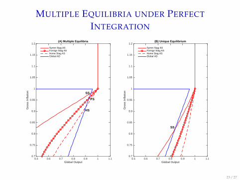
MULTIPLE EQUILIBRIA UNDER PERFECT

INTEGRATION

Global Output0.5 0.6 0.7 0.8 0.9 1 1.1

Gro

ss In

flatio

n

0.7

0.75

0.8

0.85

0.9

0.95

1

1.05

1.1

1.15

1.2(A) Multiple Equilibria

Symm Stag ASForeign Stag ASHome Stag ASGlobal AD

Global Output0.5 0.6 0.7 0.8 0.9 1 1.1

Gro

ss In

flatio

n

0.7

0.75

0.8

0.85

0.9

0.95

1

1.05

1.1

1.15

1.2(B) Unique Equilibrium

Symm Stag ASForeign Stag ASHome Stag ASGlobal AD

FS

SS

HS

SS

23 / 27

CURRENCY WARS

Nominal exchange rate:

St =P∗

tPt

∆St =Π∗

tΠt

Exchange rate policy when rw,Nat < 0:I A pegged exchange rate St = S̄ eliminates any asymmetric

stagnation equilibrium

I Benefits the nation in stagnation at the expense of the nation notin stagnation

I Sufficiently aggressive depreciation eliminates the symmetricstagnation as equilibrium

24 / 27

CONCLUSIONS FOR POLICY

1. Importance of a policy responseI ZLB can persist for arbitrarily long periods

2. Importance of fiscal policy coordinationI Fiscal expansions will tend to be undersupplied

I Fiscal austerity will tend to be oversupplied

3. Risks of beggar-thy-neighbor policiesI Exchange rate policies may alleviate stagnation in one country

while worsening in the other

I Structural reform and targeting trade surplus similar effects

4. Fiscal policy focused on diminishing oversupply of saving

25 / 27

Additional Slides

26 / 27

SECULAR STAGNATION EPISODES

4.55  

4.65  

4.75  

4.85  

4.95  

5.05  

5.15  

1990   1993   1996   1999   2002   2005   2008   2011  

United  States  

GDP  per  capita  

Real  GDP  per  Capita  

Projected  Output  

PotenCal  Output  

Model  Output  per  Capita  

0.0%  

1.0%  

2.0%  

3.0%  

4.0%  

5.0%  

6.0%  

7.0%  

2000   2002   2004   2006   2008   2010   2012   2014  

Interest  Rate  

0.0%  

0.5%  

1.0%  

1.5%  

2.0%  

2.5%  

2000   2002   2004   2006   2008   2010   2012   2014  

Infla/on  Rate  

5.30  

5.50  

5.70  

5.90  

6.10  

6.30  

1970   1975   1980   1985   1990   1995   2000   2005   2010  

Japan  

GDP  per  capita,  1970-­‐2013  

Pre-­‐Stagna<on  Trend  

Poten<al  Output  -­‐  Model  

Output  -­‐  Model  

0.0%  

1.0%  

2.0%  

3.0%  

4.0%  

5.0%  

6.0%  

7.0%  

8.0%  

1986   1990   1994   1998   2002   2006   2010  -­‐1.5%  

-­‐1.0%  

-­‐0.5%  

0.0%  

0.5%  

1.0%  

1.5%  

2.0%  

2.5%  

3.0%  

1986   1990   1994   1998   2002   2006   2010  

4.55  

4.60  

4.65  

4.70  

4.75  

4.80  

4.85  

4.90  

4.95  

5.00  

1995   1997   1999   2001   2003   2005   2007   2009   2011   2013  

Eurozone

 

Data  

Pre-­‐Stagna;on  Trend  

Poten;al  Output  

Output  

0.0%  

0.5%  

1.0%  

1.5%  

2.0%  

2.5%  

3.0%  

3.5%  

4.0%  

4.5%  

5.0%  

2002   2004   2006   2008   2010   2012   2014  -­‐0.5%  

0.0%  

0.5%  

1.0%  

1.5%  

2.0%  

2.5%  

3.0%  

3.5%  

2002   2004   2006   2008   2010   2012   2014  

Back

27 / 27