HAL Id: hal-01414179https://hal.inria.fr/hal-01414179v2

Submitted on 4 Mar 2017

HAL is a multi-disciplinary open accessarchive for the deposit and dissemination of sci-entific research documents, whether they are pub-lished or not. The documents may come fromteaching and research institutions in France orabroad, or from public or private research centers.

L’archive ouverte pluridisciplinaire HAL, estdestinée au dépôt et à la diffusion de documentsscientifiques de niveau recherche, publiés ou non,émanant des établissements d’enseignement et derecherche français ou étrangers, des laboratoirespublics ou privés.

A consolidated perspective on multi-microphone speechenhancement and source separation

Sharon Gannot, Emmanuel Vincent, Shmulik Markovich-Golan, AlexeyOzerov

To cite this version:Sharon Gannot, Emmanuel Vincent, Shmulik Markovich-Golan, Alexey Ozerov. A consolidated per-spective on multi-microphone speech enhancement and source separation. IEEE/ACM Transactionson Audio, Speech and Language Processing, Institute of Electrical and Electronics Engineers, 2017,25 (4), pp.692-730. 10.1109/TASLP.2016.2647702. hal-01414179v2

1

A Consolidated Perspective on Multi-MicrophoneSpeech Enhancement and Source Separation

Sharon Gannot, Emmanuel Vincent, Shmulik Markovich-Golan, and Alexey Ozerov

Abstract—Speech enhancement and separation are core prob-lems in audio signal processing, with commercial applicationsin devices as diverse as mobile phones, conference call systems,hands-free systems, or hearing aids. In addition, they are cru-cial pre-processing steps for noise-robust automatic speech andspeaker recognition. Many devices now have two to eight mi-crophones. The enhancement and separation capabilities offeredby these multichannel interfaces are usually greater than thoseof single-channel interfaces. Research in speech enhancementand separation has followed two convergent paths, startingwith microphone array processing and blind source separation,respectively. These communities are now strongly interrelatedand routinely borrow ideas from each other. Yet, a comprehensiveoverview of the common foundations and the differences betweenthese approaches is lacking at present. In this article, we proposeto fill this gap by analyzing a large number of establishedand recent techniques according to four transverse axes: a)the acoustic impulse response model, b) the spatial filter designcriterion, c) the parameter estimation algorithm, and d) optionalpostfiltering. We conclude this overview paper by providing a listof software and data resources and by discussing perspectives andfuture trends in the field.

Index Terms—Multichannel, array processing, beamforming,Wiener filter, independent component analysis, sparse componentanalysis, expectation-maximization, postfiltering.

I. INTRODUCTION

SPEECH enhancement and separation are core problems inaudio signal processing. Real-world speech signals often

involve one or more of the following distortions: reverberation,interfering speakers, and/or noise. In this context, sourceseparation refers to the problem of extracting one or moretarget speakers and cancelling interfering speakers and/ornoise. Speech enhancement is more general, in that it refersto the problem of extracting one or more target speakers andcancelling one or more of these three types of distortion. Ifone focuses on removing interfering speakers and noise, asopposed to reverberation, the terms of “signal enhancement”and “source separation” become essentially interchangeable.These problems arise in various real scenarios. For instance,spoken communication over mobile phones or hands-freesystems requires the enhancement or separation of the near-end speaker’s voice with respect to interfering speakers andenvironmental noises before it is transmitted to the far-endlistener. Conference call systems or hearing aids face the sameproblem, except that several speakers may be considered as

S. Gannot and S. Markovich-Golan are with Bar-Ilan University, Ramat-Gan5290002, Israel (email: gannot@eng.biu.ac.il, shmuel.markovich@biu.ac.il).E. Vincent is with Inria, 54600 Villers-les-Nancy, France (e-mail: em-manuel.vincent@inria.fr). A. Ozerov is with Technicolor R&D, 35576 CessonSevigne, France (email: alexey.ozerov@technicolor.com).

targets. Speech enhancement and separation are also crucialpre-processing steps for robust automatic speech recognitionand understanding, as available in today’s personal assistants,GPS, televisions, video game consoles, and medical dictationdevices. More generally, they are believed to be necessary toprovide humanoid robots, assistive devices, and surveillancesystems with machine audition capabilities. While the aboveapplications require real-time processing, off-line separation ofsinging voice, drums, and other musical instruments has beensuccessfully used for music information retrieval, upmixing ofmono or stereo movie soundtracks to 3D sound formats, andremixing of music recordings. Other applications, e.g. meetingtranscription, can be also processed off-line.

With few exceptions such as speech codecs and old soundarchives, the input signals are multichannel. The number ofmicrophones per device has steadily increased in the lastfew years. Most smartphones, tablets and in-car hands-freesystems are now equipped with two or three microphones.Hearing aids typically feature two microphones per ear anda wireless link [1] to enable communication between the leftand right hearing aids, and conference call systems with eightmicrophones are commercially available. Research prototypeswith forty to hundreds of microphones have been demonstratedin lecture halls, office and domestic environments [2]–[6].The enhancement capabilities offered by these multichannelinterfaces are usually greater than those of single-channel in-terfaces. They make it possible to design multichannel spatialfilters that selectively enhance or suppress sounds in certaindirections (or volumes) by exploiting the spatial diversity, e.g.phase and level differences, or more generally, the differentacoustic properties between channels. Single-channel spectralfilters, in contrast, require much more detailed knowledgeabout the target and the noise and they usually result in smallerquality improvement. As a matter of fact, it can be shown thatthe maximum quality improvement theoretically achievablewith only two microphones is already much greater than witha single microphone and that it keeps increasing with moremicrophones [7].

Hundreds of multichannel audio signal enhancement tech-niques have been proposed in the literature over the last fortyyears along two historical research paths. Microphone arrayprocessing emerged from the theory of sensor array processingfor telecommunications and it focused mostly on the local-ization and enhancement of speech in noisy or reverberantenvironments [8]–[12], while blind source separation (BSS)was later popularized by the machine learning communityand it addressed “cocktail party” scenarios involving severalsound sources mixed together [13]–[18]. These two research

2

tracks have converged in the last decade and they are hardlydistinguishable today. As will be shown in this overview paper,source separation techniques are not necessarily blind anymoreand most of them exploit the same theoretical tools, impulseresponse models and spatial filtering principles as speechenhancement techniques.

Despite this convergence, most books and reviews havefocused on either of these tracks. This article intends to fill thisgap by providing a comprehensive overview of their commonfoundations and their differences. The vastness of the topicrequires us to limit the scope of this overview to the following:

• we focus on multichannel recordings made by multiplemicrophones, as opposed to multichannel signals createdby mixing software which do not match the acoustics ofreal environments;

• we mostly study the enhancement and separation ofspeech with respect to interfering speech sources andenvironmental noise in reverberant environments, as op-posed to cancelling echoes and reverberation of the targetspeech;

• we concentrate on truly multichannel techniques based onacoustic impulse response models and multichannel filter-ing: as such, we only briefly introduce speech and noisemodels, computational auditory scene analysis (CASA)models, and time-frequency masking techniques used toassist multichannel processing, but do not describe theiruse for single-channel or channel-wise filtering in depth;

• we do not describe possible use of the enhanced signalsfor subsequent tasks;

• time difference of arrival (TDOA) estimation and speakerlocalization of (multiple) sound sources are beyond thescope of this paper.

Readers interested in multichannel signals created by pro-fessional mixing software and in the use of source separationas a prior step to audio upmixing and remixing may referto, e.g., [19]–[21]. Echo cancellation, dereverberation, andCASA are major topics described in the books [22]–[25].For more information about advanced spectral models andtheir use for single-channel and channel-wise spectral filtering,see, e.g., [18], [26], [27]. For the use of speech enhancementand musical instrument separation as pre-processing stepsfor speech recognition and music information retrieval, see,e.g., [28]–[31]. For a survey of TDOA and location estimationtechniques, interested readers may refer to [32]–[34].

In spite of its limited scope, this overview still covers awide field of research. In order to classify existing techniquesirrespectively of their origin in microphone array processing orBSS, we adopt four transverse axes: a) the acoustic impulseresponse model, b) the spatial filter design criterion, c) theparameter estimation algorithm, and d) optional postfiltering.These four modeling and processing steps are common toall techniques, as illustrated in Fig. 1. The structure of thearticle is as follows. We recall useful elements of acousticsand introduce general notations in Section II. After describingvarious acoustic impulse response models in Section III,we define the fundamental concepts of spatial filtering inSection IV and review existing design criteria, estimation algo-

rithms, and postfiltering techniques in Sections V, VI, and VII,respectively. We provide a list of resources in Section VIII andconclude in Section IX by summarizing the similarities and thedifferences between approaches originating from microphonearray processing and BSS and discussing perspectives in thefield.

II. ELEMENTS OF ACOUSTICS — NOTATIONS

From now on, we assume that two or more sound sourcesare simultaneously recorded by two or more microphones.The microphones are assumed to be omnidirectional, unlessexplicitly stated otherwise. The set of microphones is calleda microphone array. Each recorded signal is called a channeland the set of recorded signals is the array input signal or themixture signal.

A. Physics

Sound is a variation of air pressure on the order of 10−2 Pafor a speech source at a distance of 1 m, on top of the averageatmospheric pressure of 105 Pa. For such pressure values, thewave equation that governs the propagation of sound in air islinear [35]. This has two implications:

1) the pressure field at any time is the sum of the pressurefields resulting from each source at that time;

2) the pressure field emitted at a given source propagatesover space and time according to a linear operation.

Unless clipping occurs, microphones operate linearly to recordthe pressure value at given point in space. If one considers thepressure field emitted by each source as the target1, the overallphenomenon is therefore linear.

In the free field, the solution to the wave equation is givenby the spherical wave model. The waveform xi(t) recorded atpoint i when emitting a waveform sj(t) at point j is equal to

xi(t) =1√

4πqijsj

(t− qij

c

)(1)

with t denoting continuous time, qij the distance betweenpoints i and j, and c the speed of sound, that is 343 m/s at20C. This speed is very small compared to the speed of light,so that propagation delays are not negligible. The recordedwaveform differs from the emitted waveform by a delay qij/cand an attenuation factor of 1/

√4πqij .

In the presence of obstacles, the sound wave is affected indifferent ways depending on its frequency ν. The wavelengthλ = c/ν of audio varies from 17 mm at ν = 20 kHz to 17 mat ν = 20 Hz.

When the sound wave hits an object of dimension smallerthan λ, it is not affected. When it hits an obstacle of compara-ble dimension to λ, it is subject to diffraction. The wavefrontis bended in a way that depends on the shape of the obstacle,its material and the angle of incidence. Roughly speaking, itwill take more time for the wave to pass the obstacle and itwill be more attenuated than in air. This phenomenon occurs

1Loudspeakers and musical instruments such as the trumpet do not operatelinearly. These nonlinearities occur within solid parts of the loudspeaker orthe instrument, however, before vibration is transmitted to air.

3

sourcesignals

Roomacoustics

(Sec. II and III)

multichannelmixture signal

filteredsignal

postfilteredsignal

Spatialfiltering

(Sec. IV and V)

Postfiltering(Sec. VII)

Parameterestimation

(Sec. VI)

Figure 1. General schema showing acoustical propagation (gray) and the processing steps behind speech enhancement and source separation (black). Plainarrows indicate the processing order common to all algorithms and dashed arrows the feedback loops for certain algorithms.

most notably for hearing aid users, whose torso, head, andpinna, act as obstacles [36]. It also explains source directivity,i.e. the fact that the sound emitted by a source depends ondirection.

When the wave hits a large rigid surface of dimension largerthan λ, it is subject to reflection. The direction of the reflectedwave is symmetrical to the direction of the incident wave withrespect to the surface normal. Only part of the wave power isreflected: the rest is absorbed by the surface. The absorptionratio depends on the material and the angle of incidence [37].It is on the order of 1% for a tiled floor, 7% for a concretewall, and 15% for a carpeted floor.

Due to these small values, many successive wave reflectionstypically occur before the power becomes negligible. Thisinduces multiple propagation paths between each source andeach microphone, each with a different delay and attenuationfactor. The waves corresponding to different paths are coherentand may result in constructive or destructive interference.

B. Deterministic perspective

Let us now move from the physical domain to discrete timesignal processing. We assume that the recorded sound sceneconsists of J sources and that the number of microphones isequal to I . We adopt the following general notations: scalarsare represented by plain letters, vectors by bold lowercaseletters, and matrices by bold uppercase letters. The sourceindex, the microphone index, and the time index are denotedby i, j, and t, respectively. The operator T refers to matrixtransposition, and H to Hermitian transposition.

According to the first linearity assumption in Section II-A,the multichannel mixture signal x(t) = [x1(t), . . . , xI(t)]

T

can be expressed as

x(t) =

J∑

j=1

cj(t) (2)

where cj(t) = [c1j(t), . . . , cIj(t)]T is the spatial image [38]

of source j, that is the contribution of that source to thesound recorded at the microphones. This formulation is verygeneral: it applies both to targets and noise, and multiple noisesounds can be modeled either as multiple sources or as a singlesource [39]. In particular, it is valid for spatially diffuse sourcessuch as wind, trucks, or large musical instruments, which emitsound in a large region of space.

In the case of a point source, the second linearity assump-tion makes it possible to express cj(t) by linear convolu-tion of a single-channel source signal sj(t) and the vectoraj(t, τ) = [a1j(t, τ), . . . , aIj(t, τ)]T of acoustic impulse re-sponses (AIRs) from the source to the microphones:

cj(t) =

∞∑

τ=0

aj(t, τ)sj(t− τ) (3)

This expression only holds for sources such as human speakerswhich emit sound in a tight region of space. The AIRs resultfrom the summation of the multiple propagation paths andthey vary over time due to movements of the source, of themicrophones, or of other objects in the environment. Whensuch movements are small, they can be approximated as time-invariant and denoted as aj(τ).

A schematic illustration of the shape of an AIR is providedin Fig. 2. It consists of three successive parts. The first peak isthe direct path from the source to the microphone, as modeledin (1). It is followed by early echoes corresponding to thefirst few reflections on the room boundaries and the furniture.Subsequent reflections cannot be distinguished from each otheranymore and they form an exponentially decreasing tail calledreverberation. This overall shape is often described by twoquantities: the reverberation time (RT), that is the time it takesfor the reverberant tail to decay by 60 decibels (dB), and thedirect-to-reverberant ratio (DRR), that is ratio of the powerof direct sound (i.e., direct path) to that of the rest of theAIR. The RT depends solely on the room, while the DRRalso depends on the source-to-microphone distance. The RTis virtually equal to 0 in outdoor conditions due to the absenceof reflection and it is on the order of 50 ms in a car [40], 0.2to 0.8 s in office or domestic conditions, 0.4 s to 1 s in aclassroom, and 1 s or more in an auditorium [41].

Fig. 3 depicts a real AIR measured in a meeting room. It hasboth positive and negative values and it exhibits a strong firstreflection on a table just after the direct path, but its magnitudefollows the overall shape in Fig. 2.

C. Statistical perspective

Besides the above deterministic characterization of AIRs, itis useful to adopt a statistical point of view [35], [42]. To doso, we decompose AIRs as

aij(τ) = eij(τ) + rij(τ) (4)

4

0 20 40 60 80 1000

0.1

0.2

0.3

0.4

0.5

direct path

early echoes

reverberation

τ (ms)

magnitude

Figure 2. Schematic illustration of the shape of an AIR for a reverberationtime of 0.25 s (from [18]).

0 20 40 60 80 100

−0.2

−0.1

0

0.1

0.2

0.3

0.4

0.5

τ (ms)

aij(τ)

Figure 3. First 0.1 s of a real AIR from the Aachen Impulse ResponseDatabase [41] recorded in a meeting room with a reverberation time of 0.23 swith a source-to-microphone distance of 1.45 m.

where eij(τ) models the direct path and early echoes andrij(τ) models reverberation.

The fact that reverberation results from the superposition ofthousands to millions of acoustic paths makes it follow the lawof large numbers. This implies three useful properties. Firstly,rij(τ) can be modeled as a zero-mean Gaussian noise signalwhose amplitude decays exponentially over time according tothe room’s RT [43]. Secondly, the covariance E(rij(ν)r∗ij(ν

′))between its Fourier transform rij(ν) at two different frequen-cies ν and ν′ decays quickly with the difference between νand ν′ [44], [45]. Thirdly, if the room’s RT is large enough, thereverberant sound field is diffuse, homogenous and isotropic,which means that it has equal power in all directions of space.This last property makes it possible to compute the normalizedcorrelation between two different channels i and i′ in closed-form as [35], [45], [46]

Ωii′(ν) =Espat(rij(ν)r∗i′j(ν))√

Espat(|rij(ν)|2)√

Espat(|ri′j(ν)|2)

=sin(2πν`ii′/c)

2πν`ii′/c(5)

where Espat denotes spatial expectation over all possible abso-lute positions of the sources and the microphone array in the

0 1 2 3 4 5 6 7 8

−0.2

0

0.2

0.4

0.6

0.8

1

ν (kHz)

Ωii′(ν)

ℓii′ = 5 cm

ℓii′ = 20 cm

ℓii′ = 1 m

Figure 4. Interchannel coherence Ωii′ (ν) of the reverberant part of an AIRas a function of microphone distance `ii′ and frequency ν.

room, and `ii′ the distance between the microphones. Notethat the result does not depend on j anymore. This quantityknown as the interchannel coherence is shown in Fig. 4. Itis large for small arrays and low frequencies and it increaseswith microphone distance and frequency. We can further definethe I × I coherence matrix of the diffuse sound field byconcatenating all elements from (5) as (Ω(ν))ii′ = Ωii′(ν).It is interesting to note that both deterministic and statisticalperspectives are valid. The appropriate choice depends on theobservation length, and both perspectives can be useful inaccomplishing different tasks [47]. We will elaborate on thisissue in the subsequent section.

III. ACOUSTIC IMPULSE RESPONSE MODELS

The above properties of AIRs can be modeled and exploitedto design enhancement techniques. Five categories of modelshave been proposed in the literature. A model is defined bya parameterization of the AIRs and possible prior knowledgeabout the parameter values. This prior knowledge can take theform of deterministic constraints, penalty terms which we shalldenote by P(.), or probabilistic priors which we shall denoteby p(.).

A. Time-domain models

The simplest approach is to consider the AIRs as finiteimpulse response (FIR) filters modeled by their time-domaincoefficients aj(t, τ) or aj(τ), τ ∈ 0, . . . , L−1. The assumedlength L is generally on the order of several hundred to afew thousand taps. This model was very popular in the earlystages of research [48]–[55]. Recently, interest has revivedwith sparse penalties which account for prior knowledge aboutthe physical properties of AIRs, namely the facts that powerconcentrates in the direct path and the first early echoes [56]–[60] and that the time envelope decays exponentially [61], butthese penalties have not yet been used in a BSS context.

Time-domain modeling of AIRs exhibits several limitations.Firstly, prior knowledge about the spatial position of thesources does not easily translate into constraints on the AIRcoefficients [62]. Secondly, the source signals are typically

5

modeled in the time-frequency domain instead, which forcesestimation algorithms to alternate between one domain and theother [63]. Finally, the large number of parameters involvedtranslates into large computational cost [64].

B. Narrowband approximationTo address these limitations, the convolution in the time

domain can be approximated by a multiplication in the short-time Fourier transform (STFT) domain [65], provided that theframe length is sufficiently large. Let us denote by cj(n, f)and sj(n, f) the STFT of cj(t) and sj(t), respectively, withn ∈ 1, . . . , N the frame index, f ∈ 0, . . . , F − 1 thediscrete frequency bin, N the number of time frames andF the discrete Fourier transform (DFT) length. The so-callednarrowband approximation [66]–[72] is given by

cj(n, f) = aj(n, f)sj(n, f) (6)

where aj(n, f) = [a1j(n, f), . . . , aIj(n, f)]T is the concate-nation of the acoustic transfer functions (ATFs) from source jto the microphones. The appropriate frame length with respectto the length of the AIR is determined in [7], [73]. The ATFscan be either time-varying or time-invariant. In the formercase, they can be represented via a dynamical model [74]. Inthe latter case, they simplify to aj(n, f) = aj(f).

The narrowband approximation significantly simplifies esti-mation algorithms, since the decoupling between frequenciesreduces the dimension of the problem. However, it may raiseother problems, most notably gain ambiguity and permutationambiguity. These ambiguities can be mitigated by smoothingbetween nearby frequencies [75], [76] or by introducing ge-ometrical (soft or hard) constraints [70], [77], [78]. Interest-ingly, the latter references demonstrate the common founda-tions of microphone array and BSS methods for separatingspeech sources in reverberant environments.

These constraints are based on the fact that, in the absenceof echoes and reverberation, the vector of ATFs simplifies tothe steering vector, that is the DFT of (1):

dj(f) =[

1√4πq1j

e−2πq1jνf/c, . . . ,1√

4πqIje−2πqIjνf/c

]T(7)

with =√−1, νf = f × fs/F the continuous frequency (in

Hz) corresponding to frequency bin f ∈ 0, . . . , F/2, and fsthe sampling frequency. A case of practical interest is the so-called far-field case, when the source-to-microphone distancesqij are large compared to the inter-microphone distances `ii′ .The attenuation factors 1/

√4πqij are then considered as equal,

and the steering vector further simplifies (up to this factor) to

dj(f) =[e−2πq1jνf/c, . . . , e−2πqIjνf/c

]T. (8)

An explicit model of early echoes was also recently proposedin [79].

C. Relative transfer function and interchannel modelsAn alternative approach to handle the gain ambiguity is to

consider the relative transfer function (RTF) between channels

for a given source. Taking the first microphone as a reference,the vector of RTFs aj(f) = [a1j(f), . . . , aIj(f)]T for sourcej is defined as [69]

aj(f) ,1

a1j(f)aj(f). (9)

A variant of this representation is to normalize the amplitudeand the phase of the ATFs as [80], [81]

aj(f) =e−∠a1j(f)

‖aj(f)‖ aj(f). (10)

The amplitude normalization in (10), which was also consid-ered in [66], is more robust than in (9) since the normalizationfactor depends on all channels. The phase normalizationremains sensitive to the choice of the reference microphone,though. For a soft selection of the reference channel pleaserefer to [82]. For generalizations of the RTF, see [83], [84].

The RTF encodes the interchannel level difference (ILD),also known as the interchannel intensity difference (IID), indecibels and the interchannel time difference (ITD) in secondsat each frequency [85]:

ILDij(f) = 20 log10 |aij(f)| (11)

ITDij(f) =∠aij(f)

2πνf(12)

where ∠ denotes the phase in radians of a complex number.The ITD is unambiguously defined only below the frequencyc/`i1, known as the spatial aliasing frequency, with `i1 thedistance between microphones i and 1. With a sampling rateof 16 kHz, this corresponds to a sensor spacing of less than4.3 cm. Above that frequency, the phase difference becomeslarger than 2π and the ITD can be measured only up to aninteger multiple of 1/νf . For that reason, the interchannelphase difference (IPD)

IPDij(f) = ∠aij(f) (13)

is often considered instead.

This model is popular for channel-wise filtering in thecontext of CASA, where the ILD and ITD are called interaurallevel and intensity differences, respectively, and are influencedby the shape of the pinna, the head and the torso [36]. Ithas however been used for multichannel filtering too [71],[85]–[87]. The use of level and phase differences retainsthe information about the source positions while discardingabsolute levels and phases which are considered as irrelevant.Indeed, in the absence of echoes and reverberation, the ITD atall frequencies becomes equal to the TDOA (qij − q1j)/c, thevector of RTFs becomes equal to the relative steering vector

dj(f) =[1, e−2π(q2j−q1j)νf/c, . . . , e−2π(qIj−q1j)νf/c

]T,

(14)and the normalized vector of ATFs aj(f) becomes equal tothe steering vector dj(f) normalized as in (10). This has beenexploited to constrain aj(f) in anechoic conditions [88], [89]and to derive penalties over aj(f) [85], [90] or aj(f) [81] in

6

reverberant conditions, such as

P(aj |dj) =

F−1∑

f=0

‖aj(f)− dj(f)‖. (15)

It should be noted however that such penalties do not match theactual distribution of ILD and IPD in the presence of echoesand reverberation [18, Fig. 2]. The preservation of interauralquantities is especially important in hearing aids, in order toincrease speech intelligibility [91] and preserve the spatialawareness of the wearer. For penalties specifically designedfor this application area, see [92]–[99].

D. Inter-frame and inter-frequency models

As mentioned above, the narrowband approximation holdsonly when the frame length is sufficiently long. Time-domainfiltering can be exactly implemented in the frequency domainusing overlap and save techniques [69], [100], provided thatthe analysis frame-length is larger than the filter length.However, this framework necessitates rectangular windows ofdifferent length in the analysis and synthesis stages. This mightlimit the performance of the separation algorithms, especiallyin dynamic scenarios.

In the conventional STFT domain [65], [101], [102], it canbe shown that time-domain convolution by time-invariant AIRstranslates into inter-frame and inter-band convolution [103],[104]:

cj(n, f) =

F−1∑

f ′=0

∑

n′

aj(n′, f ′, f)sj(n− n′, f ′). (16)

Since this expression involves multiple filtering operations, itis beneficial to consider the subband filtering approximation:

cj(n, f) =∑

n′

aj(n′, f)sj(n− n′, f) (17)

which was used to derive speech enhancement and separationalgorithms in [105], [106]. Suitable DFT zero-padding makesit equivalent to time-domain filtering [107]–[109], however itintroduces a coupling between frequencies. These models havebeen little used in practice, due to the potentially large numberof STFT domain filter coefficients to be estimated.

E. Full-rank covariance model

An alternative approach which partly overcomes the limita-tions of the narrowband approximation is to model the second-order statistics of the ATFs. Let us consider the narrowband ap-proximation (6) and assume that the source STFT coefficientssj(n, f) have a zero-mean nonstationary Gaussian distributionwith variance σ2

sj (n, f), and they are all independent source-,frame- and frequency-wise (i.e., over j, n and f ). Under thislocal Gaussian model (LGM) [110]–[112], it can be shownthat the source spatial images cj(n, f) follow a zero-meanmultivariate nonstationary Gaussian distribution

p(cj(n, f)|Σcj (n, f)) =e−cHj (n,f)Σ−1

cj(n,f)cj(n,f)

|πΣcj (n, f)| (18)

with covariance matrix

Σcj (n, f) = σ2sj (n, f)Rj(n, f) (19)

where Rj(n, f) is the so-called spatial covariance ma-trix [113]. Under the narrowband approximation, Rj(n, f) =aj(n, f)aHj (n, f) is constrained to be a rank-1 matrix. Thisimplies that the channels of cj(n, f) are coherent, i.e. perfectlycorrelated.

It was proposed in [113] to relax this constraint and toconsider an unconstrained, full-rank spatial covariance matrixRj(n, f) within the LGM instead. This more flexible formu-lation is applicable to diffuse sources or reverberated sourceswhose AIRs are longer than the frame length. In such cases,the sound field spans several directions at each frequency, suchthat the channels of cj(n, f) become incoherent. The diagonalentries of Rj(n, f) encode the ILD and its off-diagonal entriesencode the IPD and the interchannel coherence (IC), that isthe correlation between channels.

The spatial covariance can be either time-varying or time-invariant. In the former case, it can be represented via adynamical model [114]. In the latter case, it simplifies toRj(n, f) = Rj(f).

Due to the increased number of parameters, the estimationof this model is more difficult, especially when the number ofmicrophones I is large. To overcome this difficulty, several ap-proaches have proposed to constrain the full-rank model basedon physical AIR characteristics, microphone array geometry,and/or presumed source positions. These constraints are in-corporated either via deterministic constraints [113], [115] orprobabilistic prior distributions [116] on the model parameters.In [115], Rj(f) is represented as the weighted sum of rank-1kernels modeling individual uniformly distributed directions.In [116], the following inverse-Wishart prior is set on Rj(f)instead:

p(Rj(f)|Ψj(f),m) =

|Ψj(f)|m|Rj(f)|−(m+I)e−tr[Ψj(f)R−1j (f)]

πI(I−1)/2∏Ii=1 Γ(m− i+ 1)

(20)

where Γ(·) is the gamma function, m is the number of degreesof freedom, and Ψj(f) = (m− I)Rj(f) is the inverse scalematrix. Under certain assumptions, the mean value Rj(f) ofthis distribution can be defined as

Rj(f) = dj(f)dHj (f) + σ2revΩ(f) (21)

where dj(f) is the steering vector in (7), Ω(f) is the covari-ance matrix of a diffuse sound field whose entries Ωii′(νf )are given in (5), and σ2

rev is the power of early echoesand reverberation [113]. It was shown that, when the RT ismoderate or large, the variance of this distribution is small sothat Rj(f) is similar to Rj(f).

F. Discussion

In summary, various AIR models can be derived from thedeterministic and statistical perspectives laid in Sections II-Band II-C, respectively, depending on the frame length. Longframe lengths yield the deterministic narrowband or rank-1

7

model. As we shall see, up to I − 1 directional noise sourcescan then be perfectly eliminated in theory by narrowbandspatial filtering. However, the large number of frequency bandsand the small number of observed time frames make it difficultto estimate the appropriate filter in practice. Shorter framelengths result in the statistical full-rank spatial covariancemodel instead. The amount of directional noise cancellation isthen limited. However, this allows for low-latency processingand increases the number of frames available for the estimationof the spatial filter (see early discussion on the influenceof the frame length on the coherence [117]). These twoperspectives hence complement each other. Actually, theywere both adopted for deriving a joint noise reduction anddereverberation algorithm in [47].

IV. SPATIAL FILTERING

In this section we explore some fundamental concepts ofarray processing. Unless otherwise stated, these definitions areapplicable to all arrays (not necessarily microphone arrays).For a comprehensive review on arrays (not specifically forspeech applications), the reader is referred to [118].

A. Array Preliminaries

1) Beamformer: Assume that the far-field assumption (8)holds. A linear spatial filter is defined by a frequency-dependent vector w(f) = [w1(f), . . . , wI(f)]

T comprisingone complex-valued weight per microphone, that is applied tothe STFT x(n, f) of the array input signal x(t). Its output isequal to wH(f) x(n, f) and it can be transformed back intothe time-domain by inverse STFT.

Such a filter is called a beamformer. The term beamformeroriginally referred to direction of arrival (DOA) based filtersand was later generalized to all linear spatial filters. We willsee in Sections V-E and VII that there also exist nonlinearspatial filters, which we will simply call “spatial filters”.

2) Beampattern: In the rest of this section, we omit indexesj and f for legibility. Define a spherical coordinate system,with θ the elevation angle measured from the positive z-axis,and φ is the azimuth angle:

k = [sin(θ) cos(φ), sin(θ) sin(φ), cos(θ)]T. (22)

The radius is irrelevant for defining the classical far-fieldbeampattern.

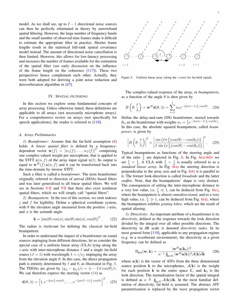
In order to understand the impact of a beamformer on soundsources impinging from different directions, let us consider thespecial case of a uniform linear array (ULA) lying along thez-axis with inter-microphone distance ` and a single far-fieldsource (J = 1) with wavelength λ = c/νf impinging the arrayfrom the elevation angle θ. In this case, the direct propagationpath is entirely determined by ` and θ, as illustrated in Fig. 5.The TDOAs are given by (qij − q1j)/c = (i − 1)` cos(θ)/c.We can therefore express the steering vector (14) as

d(θ, λ) =[1, e−2π

`λ cos(θ), . . . , e−2π(I−1)

`λ cos(θ)

]T. (23)

θ

`

i = 1i = 2i = I

Figure 5. Uniform linear array (along the z-axis) for far-field signals.

The complex-valued response of the array, or beampattern,as a function of the angle θ is then given by

B

(θ;`

λ

)= wHd(θ, λ) =

I∑

i=1

wie−2π(i−1) `λ cos(θ). (24)

Define the delay-and-sum (DS) beamformer, steered towardsθ0, as the beamformer with weights wi = 1

I e−2π(i−1) `λ cos(θ0).

In this case, the absolute squared beampattern, called beam-power, is given by∣∣∣∣B(θ;`

λ

)∣∣∣∣2

=

∣∣∣∣∣sin(Iπ `λ (cos(θ)− cos(θ0))

)

I sin(π `λ (cos(θ)− cos(θ0))

)∣∣∣∣∣

2

. (25)

Typical beampatterns as functions of the steering angle andof the ratio `

λ are depicted in Fig. 6. In Fig. 6(a)-6(b) weset `

λ = 12 . A ULA with `

λ = 12 is usually referred to as a

standard linear array. In Fig. 6(a) the steering direction isperpendicular to the array axis and in Fig. 6(b) it is parallel toit. The former look-direction is called broadside and the latterendfire. Note, that the beampatterns’ shape is very distinct.The consequences of setting the inter-microphone distance toa very low value, i.e. `

λ 1, can be deduced from Fig. 6(c),where the beampattern is almost omnidirectional, and to a veryhigh value, i.e. `

λ 1, can be deduced from Fig. 6(d), wherethe beampattern exhibits grating lobes, which are the result ofspatial aliasing.

3) Directivity: An important attribute of a beamformer is itsdirectivity, defined as the response towards the look directiondivided by the integral over all other possible directions. Thedirectivity in dB scale is denoted directivity index. In itsmost general form [119], applicable to any propagation regime(e.g. in a reverberant environment), the directivity at a givenfrequency can be defined as

Dgen(w,k) =|wHa(k0)|2

κ−1∮k∈K |wHa(k)|2A(k)dk

(26)

where a(k) is the vector of ATFs from the three dimensionalsource position k to the microphones, A(k) is the weightfor each position k in the entire space K, and k0 is thelook direction. The normalization factor of the spatial integralis defined as κ ,

∮k∈KA(k)dk. In the most familiar def-

inition of directivity, far-field is assumed. The abstract ATFparametrization is replaced by the wave propagation vector

8

0.2

0.4

0.6

0.8

1

30

210

60

240

90

270

120

300

150

330

180 0

(a) θ0 = 90o; `λ

= 12

0.2

0.4

0.6

0.8

1

30

210

60

240

90

270

120

300

150

330

180 0

(b) θ0 = 0o; `λ

= 12

0.2

0.4

0.6

0.8

1

30

210

60

240

90

270

120

300

150

330

180 0

(c) θ0 = 90o; `λ

= 132

0.2

0.4

0.6

0.8

1

30

210

60

240

90

270

120

300

150

330

180 0

(d) θ0 = 90o; `λ

= 41

Figure 6. Beampower of the DS beamformer for a ULA (along the z-axis).

in (22).The directivity in spherical coordinates is then given by

Dsph(w, φ0, θ0) =|wHd(k0)|2

14π

∫ π0

∫ 2π

0sin(θ)|B(φ, θ)|2dφdθ

(27)

with k0 = [sin(θ0) cos(φ0), sin(θ0) sin(φ0), cos(θ0)]T the

look direction of the array. Assuming that the response in thelook direction is equal to 1, this expression simplifies to [118]

Dsph(w, φ, θ) =(wHΩw

)−1(28)

where Ω is the covariance matrix of a diffuse sound fieldwhose entries Ωii′ are given in (5).

Maximizing the directivity with respect to the array weightsresults in2

Dmax(φ0, θ0) = dH(φ0, θ0)Ω−1d(φ0, θ0). (29)

As evident from this expression, the directivity may dependon the steering direction. It can be shown that the maximumdirectivity attained by the standard linear array ( `λ = 1

2 ) isequal to the number of microphones I , which is independentof the steering angle. The array weights in this case are givenby wi = 1

I , i = 1, . . . , I assuming broadside look direction.If the directivity of a beamformer significantly exceeds I , it iscalled super-directive (SD). It was also shown in [120] that foran endfire array with vanishing inter-microphone distance, i.e.`λ → 0, the directivity approaches I2. It was claimed that “it

2The array weights that maximize the directivity are given by the MVDRbeamformer (43) with Σu = Ω, which will be discussed in Section V-B.

is most unlikely” that any other beamformer can attain higherdirectivity.

4) Sensitivity: Another attribute of a beamformer is itssensitivity to array imperfections.

Let the source image at the input of the microphone arraybe c = s ·a(k0), and let u be the respective noise component.Define the source variance as σ2

s and the noise covariancematrix as Σu. The signal to noise ratio (SNR) at the outputof the microphone array is therefore given by:

SNRout =σ2s |wHa(k0)|2wHΣuw

. (30)

If the noise is spatially-white, i.e. Σu = σ2uI, then:

SNRout =σ2s

σ2u

|wHa(k0)|2wHw

= SNRin|wHa(k0)|2

wHw(31)

with SNRin =σ2s

σ2u

.Further assuming unit gain in the look direction, the SNR

improvement, denoted as white noise gain (WNG), is givenby:

WNG =1

wHw= ‖w‖−2 (32)

where ‖ • ‖ stands for the `2 norm of a vector. It was shownin [121] that the numerical sensitivity of an array, i.e. itssensitivity to perturbations of the microphone positions andto the beamformer’s weights, is inversely proportional to itsWNG:

S =1

WNG= ‖w‖2. (33)

It was further shown in [121] that there is a tradeoff betweenthe array directivity and its sensitivity and that the SD beam-former suffers from infinite sensitivity to mismatch betweenthe nominal design parameters and the actual parameters. Itwas therefore proposed to constrain the norm of w to obtain amore robust design. It should be noted that if the microphoneposition perturbations are coupled (e.g. if the microphonesshare the same packaging) a modified norm constraint shouldbe applied to guarantee low numerical sensitivity [122].

B. Array geometriesThe ULA is just one possible array geometry among many

others. In most algorithms discussed in this survey, no par-ticular array geometry is assumed. Nowadays, microphonescan be arbitrarily mounted on a device (e.g., cellphone, tablet,personal computer, hearing aid, smart watch) or several coop-erative devices. In many cases, the microphone placement isdetermined by the product design constraints rather than byacoustic considerations. Ad hoc arrays can also be formedby concatenating several devices, each of which equippedwith a small microphone array and limited processing powerand communication capabilities. Ad hoc arrays will be brieflydiscussed in IX-C3.

Despite the fact that arbitrary array constellations arewidespread, specific array geometries are still very importantand have therefore attracted the attention of both Academiaand Industry. We will now briefly describe some of thecommon microphone array geometries, namely differential andspherical microphone arrays.

9

Differential arrays [123]–[127] are small-sized arrays withmicrophone spacing significantly smaller than the speechwavelength. They implement the spatial derivative of the soundpressure field and achieve a higher directivity than regulararrays, close to that of the SD beamformer. However, thesensitivity to array imperfections is excessively high. The mostcommonly used differential arrays implement the first-orderderivative, but higher-order geometries exist. A device that candirectly measure the sound velocity, i.e. the first-order vectorderivative of the sound pressure, is also available [128].

Spherical microphone arrays [129], [130] have also at-tracted attention, due to their ability to symmetrically analyzetridimensional sound-fields [131]–[133] (see also dual-radiusspherical arrays [134]). This analysis is conveniently carriedout in the spherical harmonic domain by using the sphericalFourier transform (SFT). The interested reader is referred to arecently published book entirely dedicated to this topic [135].

Finally, crystal-shaped geometries have been used in [136].They make it possible to diagonalize the (unknown) noisecovariance matrix by a fixed, known transform, provided thatit meets an isotropy condition.

C. From geometry to linear algebra

The representation of the spatial filtering capabilities ofbeamformers as a function of the DOA is not very informativefor unstructured arrays, whose geometry does not complywith a particular structure, e.g. linear, circular or spherical.Moreover, sound propagation in a reverberant environment ismuch more intricate than in free field.

The reflections of the sound wave are captured by the AIR.From this perspective, each source can be represented as avector in a high-dimensional space whose dimension is thenumber of reflections times the number of microphones. Abeamformer can be interpreted as a linear operator in this(abstract) space. The various operations can be interpreted interms of linear algebra, without resorting to beampatterns as afunction of the DOA. One advantage of this perspective lies inthe ability to separate desired and interfering sources sharingthe same DOA [137], due to the fact that two sources with thesame DOA, but with different distances from the microphonearray, generally exhibit different reflection patterns. As previ-ously discussed, working in a very high-dimensional space isusually impractical.

It was therefore proposed both in the fields of beamformingand BSS to replace the simple steering vectors (7) and (8)by the ATFs or the respective RTFs. It was shown in [138]that the peak of the RTF in the time domain correspondsto the TDOA between the microphones, provided that theDRR is sufficiently high. Hence the RTF can be viewed asa generalization of the TDOA.

D. Fixed beamforming

The beamformers we have seen thus far are fixed beam-formers (FBFs), which only rely on the DOA or the RTFsof the target source. FBF designs are suitable when thetarget direction is known a priori, e.g., in cellphones, carsor hearing aids. In these cases, the beamformer is designed

to focus on the target source while minimizing noise andreverberation arriving from other directions. These designsrequire low computational complexity, but they may be proneto performance degradation when the microphone positionsare not accurately known (see Section IV-A). A semi-fixedbeamforming approach, suitable for cases when the positionof the target source cannot be determined in advance, isto estimate its DOA and to design a FBF steered towardsit. Alternatively, the AIRs or the RTFs between the targetsource position and the microphones can be estimated duringa calibration process and used to construct a matched-filterFBF [139].

A common FBF is the DS beamformer [140], which con-sists of averaging the delay-compensated microphone signals.Although simple, it can be shown to attain the optimaldirectivity for a spatially-white noise field. The beamwidthand sidelobe levels of the beampattern can be further con-trolled by spatial windowing of the microphone signals beforeaveraging them. This is simply implemented as a weighted-sum beamformer [141].

Considering a diffuse noise field, or scenarios where thenoise field is unknown, a beamformer which steers the beamtowards the target while minimizing the interferences arrivingfrom all other directions, can be designed [142], [143]. Inthe special case of a target located at the endfire of thearray with vanishing inter-microphone distance, the directivityof this design approaches I2 (see discussion in Sec. IV-A).In practice, due to the non-zero inter-microphone distance,the beampattern becomes frequency-dependent. While theDS beamformer has a quasi-omnidirectional beampattern atlow frequencies, the beamwidth becomes narrower at higherfrequencies. These different beamwidths result in a low-passeffect on the output signal. At very high frequencies thebeampattern is also prone to spatial aliasing (see Fig. 6). Afirst cure to this phenomenon is to split the array into subarraysthat cover different frequency bands [2], [123], [144]. In [145]the theory of frequency-invariant beampatterns for far-fieldbeamforming is developed and a practical implementation ispresented.

Eigen-filter (non-iterative) design methods for obtainingarbitrary directivity patterns using arbitrary microphones con-figurations are presented in [146]. Common iterative methodsfor FBF design, such as least squares (LS), maximum energyand nonlinear optimization, are also explored.

V. SPATIAL FILTER DESIGN CRITERIA

From now on, we focus on data-dependent spatial filters,which depend on the input signal statistics. Compared withFBFs, data-dependent designs attain higher performance dueto their ability to adapt to the actual ATFs and the statisticsof target and interfering sources. In many cases these spatialfilters are also adaptive, i.e. time-varying. However, theyusually require substantially higher computational complexity.In this section we explore many popular data-dependent spatialfilter design criteria. We start in Section V-A with a generalframework for the narrowband model and recognize severalwell-known beamforming criteria as special cases of this

10

framework. In Section V-B we elaborate on the minimum vari-ance distortionless response (MVDR) and linearly constrainedminimum variance (LCMV) beamformers, and in Section V-Con the multichannel Wiener filter (MWF) beamformer andits variant known as the speech distortion weighted multi-channel Wiener filter (SDW-MWF). We then proceed withbeamforming criteria for inter-frame, inter-frequency, or full-rank covariance models in Section V-D and spatial filter designcriteria for sparse speech models in Section V-E. All thesecriteria rely on a set of parameters such as the RTFs and thesecond order statistics of the sources, whose estimation willbe handled in Section VI.

A. General criterion for the narrowband model

Assume the narrowband approximation in the STFT do-main (6) holds. Further assume that the received microphonesignals comprise Jp point sources of interest and J−Jp noisesources with arbitrary spatial characteristics. Using (2) and (6)and the above assumptions the microphone signals are givenby:

x(n, f) = A(n, f)s(n, f) + u(n, f) (34)

where A(n, f) =[a1(n, f), . . . ,aJp(n, f)

], s(n, f) =[

s1(n, f), . . . , sJp(n, f)]T

, and u(n, f) =∑Jj=Jp+1 cj(n, f)

is the contribution of all noise sources. The frame indexn and the frequency index f are henceforth omitted forbrevity, whenever no ambiguity occurs. Denoting by Σx =ExxH the covariance matrix of the received signals, Σu =EuuH the covariance matrix of the noise signals, andΣs = diag(σ2

s1 , . . . , σ2sJp

) the covariance matrix of the signalsof interest, assumed to be mutually independent, the followingrelation holds:

Σx = AΣsAH + Σu. (35)

In the most general form, define d = QHs as the desiredoutput vector, where Q, denoted as the desired responsematrix, is a matrix of weights controlling the contributions ofthe signals of interest at all desired outputs, and d = WHx theoutputs of a filtering matrix W (note that the desired responsesare defined by Q∗). Then, the filtering matrix W is set tosatisfy the following minimum mean square error (MMSE)criterion:

WMO-MWF = argminW

E

tr(

(d− d)(d− d)H)

=

argminW

(QH −AWH)Σs(Q−WAH) + WHΣuW

(36)

where the multi-output MWF matrix, WMO-MWF, is given by:

WMO-MWF = Σ−1x AΣsQ =(AΣsA

H + Σu

)−1AΣsQ.

(37)In the more widely-used scenario, a single desired com-

bination of the signals of interest d = qHs is considered,where q, denoted as the desired response vector, is a vectorof weights controlling the contribution of the signals at thedesired output (note that the desired responses are defined byq∗). Let d = wHx be the output of a beamformer w. Thebeamformer weights are set to satisfy the following MMSE

criterion [147]:

argminw

E|d− d|2 = argminw

E|wHx− qHs|2. (38)

Several criteria can be derived from (38). Starting from thesingle desired source case Jp = 1, i.e. d = q∗s1, the MWFcan be derived by rewriting the MMSE criterion as

wMWF = argminw

∣∣q − aH1 w∣∣2 σ2

s1 + wHΣuw. (39)

The minimizer of the cost function in (39) is the celebratedMWF:

wMWF =(σ2s1a1a

H1 + Σu

)−1σ2s1a1q =

σ2s1Σ

−1u a1

1 + σ2s1a

H1 Σ−1u a1

q.

(40)The MWF cost function comprises two terms. The first

term is the power of the speech distortion induced by spatialfiltering, while the second is the noise power at the outputof the beamformer. These two terms are also known asartifacts and interference, respectively, in the source separationliterature.

To gain further control on the cost function, a tradeoffparameter may be introduced, resulting in the SDW-MWF costfunction [148]:

wSDW-MWF = argminw

∣∣q − aH1 w∣∣2 σ2

s1 + µwHΣuw

(41)

where µ is a tradeoff factor between speech distortion andnoise reduction. Minimizing the criterion in (41) yields:

wSDW-MWF =σ2s1Σ

−1u a1

µ+ σ2s1a

H1 Σ−1u a1

q. (42)

By tuning µ in the range (0,∞), the speech distortion level canbe traded for the residual noise level. For µ→∞, maximumnoise reduction but maximum speech distortion are obtained.Setting µ = 1, the SDW-MWF identifies with the MWF.Finally, for µ→ 0, the SDW-MWF identifies with the MVDRbeamformer, with a strict distortionless response wHa1 = q:

wMVDR =Σ−1u a1

aH1 Σ−1u a1

q (43)

which optimizes the following constrained minimization:

wMVDR = argminw

wHΣuw s.t. aH1 w = q

. (44)

More information regarding the SDW-MWF and MVDRbeamformers and their relations can be found in [92]. InSection VII we will discuss in details the decomposition ofthe SDW-MWF into an MVDR beamformer and a subsequentpostfiltering stage.

It is also easy to verify [118] that the MVDR and thefollowing minimum power distortionless response (MPDR)criteria are equivalent:

wMPDR = argminw

wHΣxw s.t. aH1 w = q

. (45)

The resulting beamformer

wMPDR =Σ−1x a1

aH1 Σ−1x a1

q (46)

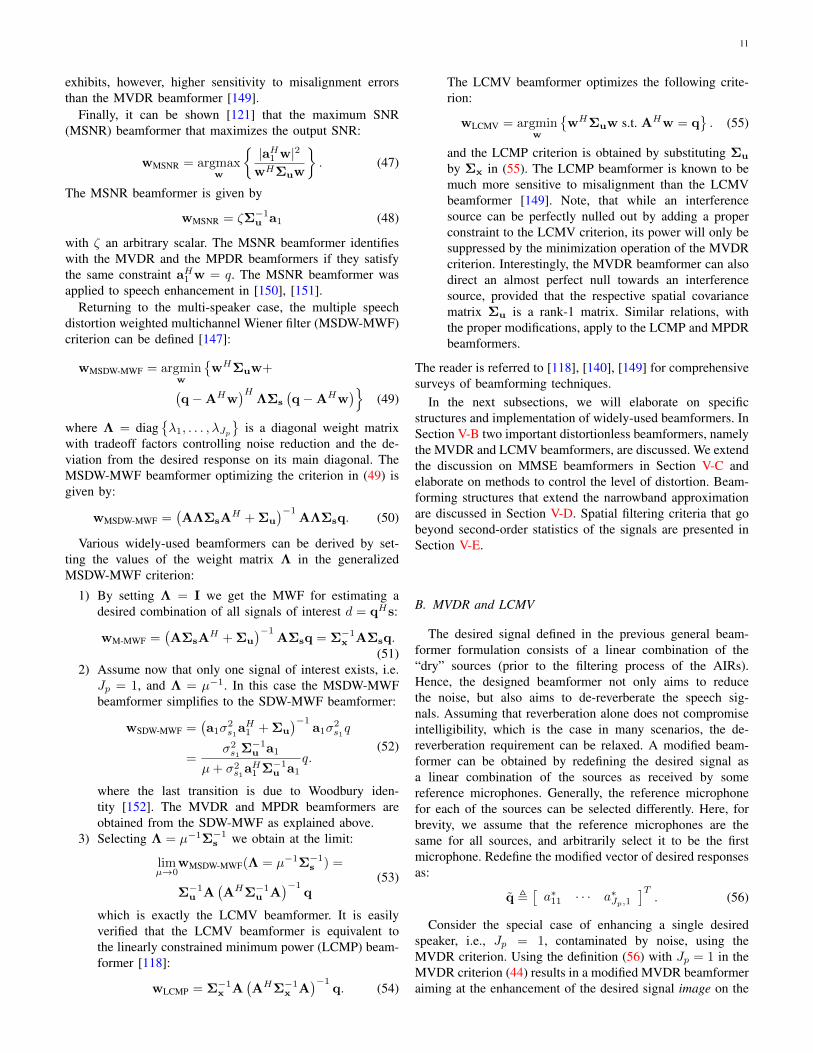
11

exhibits, however, higher sensitivity to misalignment errorsthan the MVDR beamformer [149].

Finally, it can be shown [121] that the maximum SNR(MSNR) beamformer that maximizes the output SNR:

wMSNR = argmaxw

|aH1 w|2wHΣuw

. (47)

The MSNR beamformer is given by

wMSNR = ζΣ−1u a1 (48)

with ζ an arbitrary scalar. The MSNR beamformer identifieswith the MVDR and the MPDR beamformers if they satisfythe same constraint aH1 w = q. The MSNR beamformer wasapplied to speech enhancement in [150], [151].

Returning to the multi-speaker case, the multiple speechdistortion weighted multichannel Wiener filter (MSDW-MWF)criterion can be defined [147]:

wMSDW-MWF = argminw

wHΣuw+

(q−AHw

)HΛΣs

(q−AHw

)(49)

where Λ = diagλ1, . . . , λJp

is a diagonal weight matrix

with tradeoff factors controlling noise reduction and the de-viation from the desired response on its main diagonal. TheMSDW-MWF beamformer optimizing the criterion in (49) isgiven by:

wMSDW-MWF =(AΛΣsA

H + Σu

)−1AΛΣsq. (50)

Various widely-used beamformers can be derived by set-ting the values of the weight matrix Λ in the generalizedMSDW-MWF criterion:

1) By setting Λ = I we get the MWF for estimating adesired combination of all signals of interest d = qHs:

wM-MWF =(AΣsA

H + Σu

)−1AΣsq = Σ−1x AΣsq.

(51)2) Assume now that only one signal of interest exists, i.e.

Jp = 1, and Λ = µ−1. In this case the MSDW-MWFbeamformer simplifies to the SDW-MWF beamformer:

wSDW-MWF =(a1σ

2s1a

H1 + Σu

)−1a1σ

2s1q

=σ2s1Σ

−1u a1

µ+ σ2s1a

H1 Σ−1u a1

q.(52)

where the last transition is due to Woodbury iden-tity [152]. The MVDR and MPDR beamformers areobtained from the SDW-MWF as explained above.

3) Selecting Λ = µ−1Σ−1s we obtain at the limit:

limµ→0

wMSDW-MWF(Λ = µ−1Σ−1s ) =

Σ−1u A(AHΣ−1u A

)−1q

(53)

which is exactly the LCMV beamformer. It is easilyverified that the LCMV beamformer is equivalent tothe linearly constrained minimum power (LCMP) beam-former [118]:

wLCMP = Σ−1x A(AHΣ−1x A

)−1q. (54)

The LCMV beamformer optimizes the following crite-rion:

wLCMV = argminw

wHΣuw s.t. AHw = q

. (55)

and the LCMP criterion is obtained by substituting Σu

by Σx in (55). The LCMP beamformer is known to bemuch more sensitive to misalignment than the LCMVbeamformer [149]. Note, that while an interferencesource can be perfectly nulled out by adding a properconstraint to the LCMV criterion, its power will only besuppressed by the minimization operation of the MVDRcriterion. Interestingly, the MVDR beamformer can alsodirect an almost perfect null towards an interferencesource, provided that the respective spatial covariancematrix Σu is a rank-1 matrix. Similar relations, withthe proper modifications, apply to the LCMP and MPDRbeamformers.

The reader is referred to [118], [140], [149] for comprehensivesurveys of beamforming techniques.

In the next subsections, we will elaborate on specificstructures and implementation of widely-used beamformers. InSection V-B two important distortionless beamformers, namelythe MVDR and LCMV beamformers, are discussed. We extendthe discussion on MMSE beamformers in Section V-C andelaborate on methods to control the level of distortion. Beam-forming structures that extend the narrowband approximationare discussed in Section V-D. Spatial filtering criteria that gobeyond second-order statistics of the signals are presented inSection V-E.

B. MVDR and LCMV

The desired signal defined in the previous general beam-former formulation consists of a linear combination of the“dry” sources (prior to the filtering process of the AIRs).Hence, the designed beamformer not only aims to reducethe noise, but also aims to de-reverberate the speech sig-nals. Assuming that reverberation alone does not compromiseintelligibility, which is the case in many scenarios, the de-reverberation requirement can be relaxed. A modified beam-former can be obtained by redefining the desired signal asa linear combination of the sources as received by somereference microphones. Generally, the reference microphonefor each of the sources can be selected differently. Here, forbrevity, we assume that the reference microphones are thesame for all sources, and arbitrarily select it to be the firstmicrophone. Redefine the modified vector of desired responsesas:

q ,[a∗11 · · · a∗Jp,1

]T. (56)

Consider the special case of enhancing a single desiredspeaker, i.e., Jp = 1, contaminated by noise, using theMVDR criterion. Using the definition (56) with Jp = 1 in theMVDR criterion (44) results in a modified MVDR beamformeraiming at the enhancement of the desired signal image on the

12

reference microphone a11s1:

wMVDR ,Σ−1u a1

aH1 Σ−1u a1

(57)

where a1 denotes the RTF vector of the desired source asdefined in (9). In [153] the SNR improvement of an MVDRbeamformer is evaluated as a function of the reverberationlevel at the output. It is concluded that a tradeoff betweennoise reduction and dereverberation exist, i.e. the highest SNRimprovement is obtained when dereverberation is sacrificed.

Consider the multiple speakers scenario, and assume that Jpspeakers of interest can be classified into two groups, namelyas desired or as interfering speakers. Without loss of generality,we assume that the first Jα sources are desired and denotetheir respective ATF matrix by Aα. Correspondingly, the lastJβ speakers are assumed to be interfering and their respectiveATF matrix is denoted as Aβ . The total number of sourceof interest therefore satisfies Jp = Jα + Jβ . Similarly to theabove, relaxing the dereverberation requirement, the goal ofthe beamformer is to extract the desired sources as receivedby the reference microphone while mitigating the interferingspeakers and minimizing the background noise. Explicitly, theconstraints set can be defined as

AH

w = qLCMV (58)

where A ,[

Aα Aβ

]comprises the RTFs of the desired

and interfering speakers arranged in matrices Aα and Aβ ,respectively, and qLCMV ,

[11×Jα 01×Jβ

]T. A straight-

forward computation of the LCMV beamformer requiresknowledge of the RTFs of the sources (both desired andinterfering). It can be shown (see [137]) that an equivalentconstraints set can be formulated as:

[Qα Qβ

]Hw = qLCMV (59)

where the matrices Qα and Qβ are arbitrary bases spanningthe column-subspace of the matrices Aα and Aβ , respectively,and Qα and Qβ are their normalized counterparts defined as:

Qα = diag(Qα,11, . . . , Qα,1Jα)−1Qα (60a)

Qβ = diag(Qβ,11, . . . , Qβ,1Jβ )−1Qβ . (60b)

The operator diag(·) denotes a diagonal matrix with theargument on its diagonal and Qα,1j denotes the first elementin the j-th column of the matrix Qα. Constructing the LCMVbeamformer with the constraints set in (59) can be shown to beequivalent to the construction with (58). Moreover, using (58)relaxes the requirement for estimating the RTF vectors foreach of the sources, and substitutes it with estimating twobasis matrices, one for each group of sources (desired andinterfering, respectively). A practical method for estimatingthe basis matrices Qα and Qβ is discussed in Section VI-B.

C. MWF, SDW-MWF and parametric MWF

Time-domain implementation of single-source MWF-basedspeech enhancement is proposed in [154]. The covariance ma-trix of the received microphone signals comprises speech and

noise components. Using generalized singular value decom-position (GSVD), the mixture and noise covariance matricescan be jointly diagonalized [155]. Utilizing the low-rank struc-ture of the speech component, a time-recursive and reduced-complexity implementation is proposed. The complexity canbe further reduced by shortening the length of GSVD-basedfilters.

In later work [156], a similar solution to theSDW-MWF [148] was derived from a different perspective.It is suggested to minimize the noise variance at the outputof the beamformer while constraining the maximal distortionincurred to the speech signal, denoted σ2

D. The beamformerwhich optimizes the latter criterion is called parametric MWF(PMWF):

wPMWF = argminw

wHΣuw s.t. E|d− d|2 ≤ σ2

D

(61)

The expression of the PMWF is identical to that of theSDW-MWF in (42). The relation between the parameters σ2

D

of the PMWF and µ of the SDW-MWF does not have a closed-form representation in the general case. This relation and theperformance of the PMWF are analyzed in [157].

D. Criteria for inter-frame, inter-frequency, or full-rank co-variance models

The beamformers we have seen thus far rely on the nar-rowband approximation. The underlying MMSE criterion canalso be used when this approximation does not hold, e.g., withinter-frame, inter-frequency, or full-rank covariance models.

With the full-rank covariance model in Section III-E, forinstance, the target signal to be estimated is the vector cj(n, f)of STFT coefficients of each spatial source image. Beamform-ing can then be achieved using a matrix of weights W(n, f)as cj(n, f) = WH(n, f)x(n, f). The MMSE criterion isexpressed as

argminW

E‖WH(n, f)x(n, f)− cj(n, f)‖2 (62)

and the solution is given by the MWF [113]

Wj(n, f) = Σ−1x (n, f)Σcj (n, f) (63)

with Σx(n, f) =∑Jj=1 Σcj (n, f). Variants of this criterion

involving multiple target speakers and tradeoff between speechdistortion and residual noise can be derived similarly to above.

A similar approach can also be used for the inter-frame andinter-frequency models in Section III-D. Beamformers theninvolve STFT coefficients from multiple frames or frequencybins as inputs and the MWF is obtained using a similarexpression to (63) where the covariance matrices represent thecovariance between multiple frames or frequency bins [104]–[106], [109]. In [47], the inter-frame model and the full-rank model are combined in a nested MVDR beamformingstructure.

E. Sparsity-based criteria

The beamformers we have reviewed thus far are obtainedby minimizing power criteria which can be expressed in terms

13

Magnitude STFT of a speech source sj(n, f)

n (s)

νf(kHz)

0 0.2 0.4 0.6 0.8 1

0

1

2

3

4

dB

0

10

20

30

40

50

60

0 0.5 1 1.5 2 2.5 3 3.5 4

Distribution of magnitude STFT coefficients

|sj(n, f)| (scaled to unit variance)

probab

ilitydensity

10−2

10−1

100

101

empiricalGaussian (q = 2)Laplacian (q = 1)generalized q = 0.4

Figure 7. Distribution of the magnitude STFT of a speech source.

of the second-order statistics of the signals. Mathematicallyspeaking, these statistics are sufficient to characterize Gaussiansignals. However, audio signals are often nongaussian. Fig. 7shows that, in the time-frequency domain, the distribution ofspeech signals is sparse: at each frequency, a few coefficientsare large and most are close to zero compared to a Gaussian.

This has inspired researchers to design spatial filters thattake this distribution into account. This is typically achievedby optimizing a maximum likelihood (ML) criterion under thenarrowband model (6). Three approaches have been proposed.

1) Binary masking and local inversion: A first approachconsiders that each source is active in a few time-frequencybins so that only few sources are active in each time-frequencybin. The simplest model assumes that a single source j?(n, f)is active in each time-frequency bin [85], [158], [159]. Ifwe further assume that j?(n, f) is uniformly distributed in1, . . . , J and that the noise u(n, f) is Gaussian with covari-ance Σu(f), the sources sj(n, f) and the model parametersθ = aj(f),Σu(f) can be jointly estimated by maximizingthe log-likelihood

argmaxs,θ

∑

nf

− log det(πΣu(f))

− (x(n, f)− a?j (f) s?j (n, f))H

Σ−1u (f)(x(n, f)− a?j (f) s?j (n, f)) (64)

where a?j (f) and s?j (n, f) denote the value of aj(f) andsj(n, f) for j = j?(n, f). Given j?(n, f) and θ, it turns outthat the optimal value of the predominant source is obtained by

the MVDR beamformer s?j (n, f) = wHMVDR(f)x(n, f) where

wMVDR(f) is given by (43) by identifying a1 with a?j (f)and setting q = 1. The other sources sj(n, f), j 6= j?(n, f),are set to zero. This can be interpreted as a conventionalMVDR beamformer followed by a binary postfilter equal to1 for the predominant source and 0 for the other sources (seeSection VII-A).

A variant of this approach assumes that a subset of sourcesJ (n, f) ⊂ 1, . . . , J is active in each time-frequency binwhere the number of active sources is smaller than the numberof microphones I [54], [160]–[163]. The ML criterion can thenbe written as

argmaxs,θ

∑

nf

− log det(πΣu(f))

−

x(n, f)−

∑

j∈J (n,f)

aj(f) sj(n, f)

H

Σ−1u (f)

x(n, f)−

∑

j∈J (n,f)

aj(f) sj(n, f)

. (65)

Given J (n, f) and θ, the optimal value of each active sourceis now obtained by the LCMV beamformer sj(n, f) =wH

LCMV(f)x(n, f) whose general expression is given laterin (73) where A = [aj(f)]j∈J (n,f) and q = [0, . . . , 1, . . . , 0]T

with the value 1 in the position corresponding to source j. Theactivity patterns j?(n, f) or J (n, f) and the model parametersθ can be estimated using an EM algorithm (see Section VI-C).Alternative solutions include estimating θ first using, e.g. thetechniques in Section VI-B, and subsequently looping over allpossible activity patterns and select the one yielding the largestlikelihood, or even reestimating [aj(f)]j∈J (n,f) in each time-frequency bin using other criteria than ML [163].

2) ICA and SCA: A second approach assumes that allsources are possibly active but their STFT coefficients sj(n, f)are independent and identically distributed (i.i.d.) according toa known sparse distribution. The circular generalized Gaussiandistribution is a popular choice [164], [165]. It models thephases of the source STFT coefficients as uniformly distributedand their magnitudes as [166], [167]

p(|sj(n, f)|) = qβ1/q

Γ(1/q)e−β |sj(n,f)|

q

(66)

where the parameters 0 < q < 2 and β > 0 governrespectively the shape and the variance of the prior andΓ(·) is the gamma function. This distribution includes theLaplacian (q = 1) [72], [168], [169] as a special case and itssparsity increases with decreasing q. It was shown in [164] thatq = 0.4 matches well the distribution of speech, as illustratedin Fig. 7. Generalizations of this distribution [170] and otheri.i.d. distributions [67], [76], [168], [171]–[174] have also beenused.

In the so-called determined case, when the number ofsources J is equal to the number of microphones I , estimatingthe matrix of ATFs A(f) is equivalent to estimating the matrixof beamformers W(f) = A−1(f), which can be used tojointly recover all sources as s(n, f) = WH(f)x(n, f). The

14

optimal beamformers W(f) can then be estimated in the MLsense as

WICA(f) = argmaxW(f)

∑

nf

log p(x(n, f)|A(f)) (67)

= argmaxW(f)

log |det W(f)|+∑

jnf

log p(sj(n, f))

(68)

Interestingly, this criterion is equivalent to minimizing themutual information I(s1, . . . , sJ), which is an information-theoretic measure of dependency between random vari-ables [175]. In other words, it results in maximizing the statis-tical independence of the source signals. For this reason, it wascalled nongaussianity-based independent component analysis(ICA) [176]–[178]. This is the most common form of ICA,which differs from the nonstationarity-based ICA stemmingfrom the LGM in Section III-E. Minimum mutual informationis more general than ML as it can also be applied when thedistribution p(sj(n, f)) is unknown. In practice though, mostICA methods rely on ML which is easier to optimize andcan also be applied to enhance a single source [179]. Thebeamformer resulting from nongaussianity-based ICA signifi-cantly differs from the ones we have seen so far in that it cannever be expressed in terms of the second-order statistics of thesignals. Actually, it cannot even be computed in closed-form:parameter estimation and beamforming are tightly coupled asillustrated by the dashed arrow in Fig. 1. Iterative estimationalgorithms will be reviewed in Section VI-D.

One limitation of the ICA criterion is that it is invariantwith respect to permutation of the sources. Yet, the orderof the sources must be aligned across the frequency bins.Linear constraints [70], [77] such as the one used for MVDRand penalty terms constraining aj(f) to vary smoothly overfrequency [75], [76] or to be close to the anechoic steeringvector dj(f) [78] have been used to constrain the optimiza-tion (68). Post-processing permutation alignment techniqueswhich exploit the additional fact that the source short-termspectra are correlated across frequency bands have also beenproposed [81], [180], [181].

In the so-called underdetermined case, when the number ofsources J is larger than the number of microphones I , ICAcannot recover all sources anymore and joint ML estimation ofA(f) and sj(n, f) is difficult. An approximate solution is toobtain A(f) first using, e.g. the techniques in Section VI-B3,and to subsequently estimate sj(n, f) in the ML sense:

sSCA(n, f) = argmaxs(n,f)

∑

jnf

log p(sj(n, f)) (69)

under the constraint that x(n, f) = A(f)s(n, f). Due to thesparse distribution used, this objective has been denoted sparsecomponent analysis (SCA). In the case when the generalizedGaussian distribution (66) is used, this amounts to minimizingthe sum over all sources of the q-th power of the `q norm ofeach source

∑

nf

|sj(n, f)|q

1/q

. (70)

The solution cannot be found in closed-form and requires aniterative algorithm in the general case [164], [182]. However, ifthe shape parameter q is small enough, the corresponding dis-tribution is so sparse that it forces J−I sources to zero in eachtime-frequency bin and only the remaining I sources indexedby j ∈ J (n, f) are nonzero [164]. The nonzero source STFTcoefficients are found by local inversion of the mixing process,i.e., [sj(n, f)]j∈J (n,f) = [aj(n, f)]−1j∈J (n,f)x(n, f) [72]. Thiscan be interpreted as LCMV beamforming similarly to above.The value of the noise covariance matrix Σu(f) does notmatter here since the matrix A(f) = [aj(n, f)]j∈J (n,f) isinvertible. An alternative approach that forces certain sourceSTFT coefficients to zero based on the theoretical frameworkof co-sparsity was proposed in [183].

3) Non i.i.d. models: The assumptions of independenceand identical distribution behind ICA and SCA are majorlimitations: contrary to traditional beamforming approachesbased on second-order statistics, they ignore the fact thataudio sources exhibit patterns over time and frequency. A fewapproaches have attempted to relax these two assumptions.The TRINICON framework [184] and the earlier frameworkin [185] relax the second assumption: the source signals areassumed to be independently distributed according to a sparsedistribution but the parameters of this distribution vary overtime. Independent vector analysis (IVA) [186]–[188] relaxesthe first assumption instead: it models the correlation betweenthe source STFT coefficients across frequency using a multi-variate sparse distribution, which results in the minimizationof the sum over all sources of the q-th power of the mixed`p,q norm of each source

∑

n

∑

f

|sj(n, f)|pq/p

1/q

. (71)

This model provides a principled approach to solving thepermutation problem of ICA. Mixed norms have also beenused for underdetermined separation in [63]. However, theseapproaches have little been pursued due to the limited rangeof spectro-temporal characteristics they can model and theincreased optimization difficulty.

F. Summary

In Table I a summary of important single output spatialfilters, discussed above, can be found.

VI. PARAMETER ESTIMATION ALGORITHMS ANDIMPLEMENTATION

In this section we will explore some widely-used structuresand estimation procedures for implementing the beamformersand the spatial filters discussed in Section V. We discuss thegeneralized sidelobe canceller (GSC) structure, often used forimplementing MVDR and LCMV beamformers in Sec. VI-A.The estimation of the speech presence probability (SPP), the(spatial) second-order statistics of the various signals, and theRTFs of the signals of interest are discussed in Sec. VI-B.Although, traditionally, the extraction of geometry information

15

Beamformer Criterion Solution # Hard Constraints Variants

MWF (39) (40) - SDW-MWF (42), MO-MWF (37)(63)MVDR (44) (43) 1 MPDR (46), MSNR (48)LCMV (55) (53) Jp LCMP (54)ICA (68) no closed form - TRINICON, IVA

Table ISUMMARY OF BEAMFORMERS FOR SPEECH ENHANCEMENT.

and signals’ activity patterns were only used by microphonearray processing methods, in recent years they were alsoadopted by the BSS community. We will elaborate on thedifferences and similarities of these paradigms in Sec. IX-A.Numerous statistical estimation criteria for estimating thevarious components of the spatial filters, such as maximumlikelihood (ML), maximum a posteriori (MAP), and variationalBayes (VB), are discussed in Sec. VI-C.

A. The generalized sidelobe canceller

In its most general form the LCMV beamformer optimizesthe following criterion (see also (55)):

wLCMV = argminw

wHΣuw s.t. AHw = q

(72)

where A is a general constraint matrix (not necessarily equalto the source ATFs) and q is the desired response. The criterionin (72) minimizes the noise at the beamformer output subjectto a set of linear constraints. The multiple constraint set gener-alizes the simpler MVDR criterion to allow for further controlon the beampattern, beyond the response towards the arraylook-direction. Several alternatives for constraint selection arelisted in [140], including beam derivative constraint [189],eigenvector constraint [190] and volume constraint [191].Since adaptive constrained minimization can be a cumbersometask (see e.g. [192]) it was proposed in [193] to decomposethe MVDR beamformer into separate (and orthogonal) beam-formers responsible for satisfying the constraint and for noisepower minimization. The resulting structure is called GSC.While the existence of such a decomposition was only provenfor the MVDR beamformer in [193], it was later extended tothe more general LCMV beamformer in several publications.A short and elegant proof that all LCMV beamformers can bedecomposed into a GSC structure is given in [194].

The LCMV beamformer for an arbitrary constraint matrixand a desired response vector q is given by:

wLCMV = Σ−1u A(AHΣ−1u A

)−1q. (73)

Now, the beamformer can be recast as a sum of two orthogonalbeamformers:

wLCMV = w0 −wn (74)

where w0 ∈ SpanA, wn ∈ NullA, and SpanA andNullA are respectively the column space and the null spaceof the constraint matrix A. Such an orthogonal decompositionalways exists [195]. The rank of the SpanA is Jp and therank of NullA is I − Jp. Any vector in NullA can be

further decomposed as wn = Bg. The columns of the I×(I−Jp) matrix B span NullA and g is a (I − Jp) × 1 weightvector. The matrix B is usually referred to as the blockingmatrix (BM), as it blocks all constrained signals.

Using this decomposition, the output of the beamformer isgiven by:

d = wHx = wH0 x− gH BHx︸ ︷︷ ︸

e

. (75)

The signals e = BHx, usually referred to as noise referencesignals, lie in NullA, i.e. they comprise noise-only compo-nents.

The GSC implementation hence consists of two branches,as depicted in Fig. 8. The upper branch is responsible forsatisfying the constraint set, and is usually denoted FBF.It should, however, be stressed that in some scenarios theconstraint matrix is time-varying, e.g. when the sources arefree to move. Even in such scenarios, the term FBF, althoughinaccurate, will still be used. A widely-used FBF is theperpendicular to the constraint set:

w0 = A(AHA

)−1q. (76)

Other alternatives will be discussed later.A straightforward implementation of the BM is given by

selecting the first I − Jp columns of the projection matrix tothe null subspace of A, given by:

B =(II×I − A

(AHA

)−1AH

)[ I(I−Jp)×(I−Jp)0Jp×(I−Jp)

].

(77)It is easy to verify that BHA = 0.

The role of the filters g is to minimize the noise powerat the output of the beamformer. Note that, in the idealcase, the constrained signals do not leak to the output of theBM, hence the noise power can be reduced by unconstrainedminimization. The decoupling between the application of theconstraint and the minimization of the noise power is themost important attribute of the GSC structure, emphasizing theimportance of avoiding the leakage of the constrained signalsat the output of the BM. Such a leakage contributes to the self-cancellation phenomenon, often resulting in desired signalsdistortion. The noise canceller (NC) filters g can be calculatedusing the MWF with noise reference signals e as inputs andthe output of the FBF as the desired signal:

g =(BHΣuB

)−1BHΣuw0. (78)

However, the NC is usually implemented using adaptive

16

∑ ∑

∑

e1(n, f)

e2(n, f)

eI−Jp(n, f)

dnc(n, f)

B

x1(n, f)

x2(n, f)

x3(n, f)

g1(n, f)

g2(n, f)

gI−Jp(n, f)

−

dfbf(n, f)d(n, f)+

w0

xI(n, f)

Figure 8. GSC structure for implementing the LCMV beamformer.

filters, most commonly the least mean squares (LMS) algo-rithm [196].

The GSC structure is widely used in the microphone arrayliterature. In [197] a time-domain GSC is applied to enhance adesired signal impinging the array from a fixed look-directionin a car environment. In [66], a STFT-domain subspacetracking procedure is utilized for estimating the ATFs of thedesired source (confined to a small predefined area), whichare necessary for implementing the FBF and BM blocks.The subspace tracking procedure was later utilized to addressthe multiple moving sources scenario in [198]. In [199] arobust GSC is implemented in the time domain, employingadaptive BM, constrained to a predefined DOA, and norm-constrained NC. A frequency-domain implementation of anequivalent structure is given in [200]. A GSC beamformerimplemented in the STFT domain is proposed in [69] withthe ATFs substituted by the RTFs that can be estimatedfrom the received signals utilizing speech nonstationarity. Thisstructure was extended to the two speaker case (i.e. twosources of interest: one desired and one interfering) withRTFs estimated using speech nonstationarity as well [201].Later, the multiple speaker case was addressed in [137] withthe RTFs estimated using eigenvalue decomposition (EVD).An efficient implementation of the BM with the smallestpossible number of filters can be found in [202]. The caseof multiple speakers is also addressed in [203] by assumingdisjoint activity of the various sources in the STFT domainand applying clustering procedure to localize the sources.In [204] a generalization of both the SDW-MWF and the GSC,called spatially preprocessed SDW-MWF (SP-SDW-MWF) isproposed. Applying this generalized form offers improvedrobustness to errors in the estimated RTFs.

B. SPP-based second order statistics and RTF estimation

The beamformers and the other spatial filters defined in theprevious sections assume that certain parameters are availablefor their computation, namely the RTFs of the speakers, thecovariance matrices of the background noise and the speakers,and/or the cross-covariance between the mixture signals and

the desired signal. Numerous methods exist for estimatingthese parameters. Many of them rely on estimating the SPP fordetermining noise and speech time-frequency bins combinedwith speaker classification (for the multiple speakers case) ina first stage and independently estimating the various modelparameters in a second stage. In the following, we review SPPestimation, and proceed with the estimation of covariancesmatrices and RTFs.

1) Estimating the speech presence probability: Manyspeech enhancement algorithms, implemented in the STFTdomain, require information regarding the temporal-spectralactivity of the speech signals. Contrary to the voice activitydetection (VAD) problem where low resolution is sufficient,high-resolution activity estimation in both time and frequencyis required here for proper enhancement.

We first consider the estimation of the SPP in a single-speaker scenario using a single microphone and then discussthe multi-microphone scenario. In this scenario, the STFT ofone of the microphone signals is given by:

x = c+ u (79)

where c is the spatial image of the speech source and u is thesum of all noise components. The microphone and sourcesindices are omitted for brevity and the time and frequencyindices are (n, f) unless otherwise stated. Denote the speechactivity and absence hypotheses in time-frequency bin (n, f)as Hs and Hu, respectively. The problem at hand can beviewed as a classical hypothesis testing problem.

Denote the a posteriori SNR as:

γ(n, f) ,1

|Nn| · |Ff |∑

n′∈Nn,f ′∈Ff

|x(n′, f ′)|2σ2u(n′, f ′)

. (80)

where σ2u denotes the variance of the noise component and

Nn, Ff are sets of time and frequency indices, respectively,defining a neighborhood of time-frequency points around(n, f). By averaging over a neighborhood of time-frequencypoints, the smoothness property of speech activity is utilizedto reduce fluctuations in γ, which will reduce fluctuations inthe SPP, and avoid distortion artifacts at the output of theenhancement algorithms. Assuming that the STFT coefficientsof speech and noise are Gaussian distributed and independentover time and frequency [205], γ approximately follows achi-squared distribution with r = 2|Nn| · |Ff |cdof degrees offreedom, where cdof is a correction factor resulting from thecorrelation between time and frequency bins due to the STFToverlap factor and the analysis window.

Numerous methods exist for estimating the noise powerspectral density σ2

u, e.g. by conventional spectrum estima-tion methods during speech-free time segments, by minimumstatistics [206], by the improved minima controlled recursiveaveraging [207] or by an improved MMSE criterion [208].

Let p ∈ [0, 1] denote the probability that hypothesis Hs istrue, i.e. speech is present. This probability can be calculatedas

p , P Hs|γ =Λ

1 + Λ(81)

17

where Λ is the generalized likelihood ratio, defined as

Λ ,q · P γ|Hs

(1− q) · P γ|Hs(82)

with q = P Hs the a priori probability of speech presence.

For computing Λ, we further assume that the speech poweris homogeneously distributed over the neighborhood of time-frequency bin (n, f). Define the a priori SNR as

ξ ,1

|Nn| · |Ff |∑

n∈Nn,f∈Ff

E|c(n, f)|2

σ2u(n, f)

. (83)

Using these definitions and the assumption that speech andnoise STFT coefficients are Gaussian distributed, it can beshown (see [209]) that Λ is given by

Λ =q

1− q

(1

1 + ξ

) r2

exp

(ξ

1 + ξ· r

2γ

). (84)

Substituting (84) in (81) yields

p =

1 +

1− qq

(1 + ξ)r2 exp

(− ζ

1 + ξ

r

2

)−1(85)

where

ζ , γξ. (86)

The a priori SNR and a priori SNR can be signal-dependent [210]–[212] or fixed to typical values designed tomeet certain false-alarm and miss-detection rates [209].

This approach can be extended to multichannel SPP estima-tion under the narrowband approximation [213], where multi-variate Gaussian distributions are assumed for the speech andnoise components. The resulting SPP is calculated using (85)with ζ and ξ redefined as

ξ , trΣ−1u Σc

(87)

ζ ,xHΣ−1u ΣcΣ−1u x (88)

where

Σc , AΣsAH (89)

is the covariance matrix of the images of the sources ofinterest.

Note that estimating SPP relies on estimates of SNR andconsequently the estimated power spectral densities (PSDs)of speech and noise. Straightforward incorporation of SPPin the latter power spectral density (PSD) estimates, resultsin a feedback which might increase false estimation and, insevere cases, might cause the estimated SPP to converge toone of its limits (either 0 or 1) without the ability to recover.Among possible solutions to this problem (see [206], [207]and [208]) are: 1) estimating the noise PSD independently ofthe estimated SPP; 2) using a fixed a priori SNR and fixeda priori SPP, independent of previous data-dependent SPPestimates; 3) constraining the minimal and maximal values ofthe SPP, and thus effectively limiting the period contaminatedby these errors; 4) incorporating spatial information on thespeaker in estimating the SPP (such as coherence [214] andposition [215], [216]). The latter spatial information can also

be utilized to classify the active speakers in a multiple speakersscenario.

2) Estimating second order statistics: The noise covariancematrix can be estimated by recursively averaging instantaneouscovariance matrices weighted according to the SPP:

Σu (n, f) =λ′u(n, f)Σu (n− 1, f)

+ (1− λ′u(n, f)) x(n, f)xH(n, f). (90)

where

λ′u(n, f) , (1− p(n, f))λu + p(n, f) (91)

is a time-varying recursive averaging factor and λu is selectedsuch that its corresponding estimation period ( 1

1−λu frames)is shorter than the stationarity time of the noise. Alternatively,a hard binary weighting, obtained by applying a threshold tothe SPP, can be used instead of the soft weighting.

Define the hypothesis that speaker j is present as Hsj (n, f),and its corresponding a posteriori probability as pj(n, f) ,PHsj (n, f)|x(n, f)

. Similarly to (90), the covariance ma-

trix of the spatial image of source j, denoted Σcj (n, f) ,σ2sj (n, f)aj(f)aHj (f), can be estimated by

Σcj (n, f) = λ′sj (n, f)Σcj (n− 1, f)

+ (1− λ′sj (n, f))(x(n, f)xH(n, f)− Σu (n− 1, f))

(92)

where

λ′sj (n, f) , (1− pj(n, f))λs + pj(n, f) (93)

is a time-varying recursive-averaging factor, and λs is selectedsuch that its corresponding estimation period ( 1

1−λs frames) isshorter than the coherence time of the AIRs of speaker j, i.e.the time period over which the AIRs are assumed to be time-invariant. Note that: 1) usually the estimation period is longerthan the speech nonstationarity time, therefore, although thespatial structure of Σcj (n, f) is maintained, the estimatedvariance is an average of the speech variances over multipletime periods; 2) the estimate Σcj (n, f) keeps its past valuewhen speaker j is absent.

Individual SPPs for each of the speakers can be approxi-mated from their estimated positions [215]–[217]. Given thatany of the speakers is active (i.e. hypothesis Hs is true andhence p(n, f) is high), and assuming that each time-frequencybin is dominated by at most one speaker signal (i.e. the time-frequency sparsity assumption), the a posteriori probabilitiesare obtained by

pj(n, f) = p(n, f) · PHsj |x(n, f),Hs

. (94)

Next, assuming that source position is the sufficient statisticsembedded in x(n, f) for classifying the active source weobtain:

pj(n, f) ≈p(n, f) · PHsj |r(n, f),Hs

(95)

where r(n, f) denotes position estimate of source active intime-frequency bin (n, f). A plethora of methods exist forestimating source positions, however, this topic is beyond thescope of this overview paper. By adopting a Gaussian model

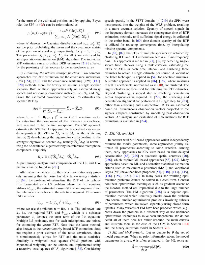
18

for the error of the estimated position, and by applying Bayesrule, the SPP in (95) can be reformulated as

pj(n, f) =p(n, f) ·πs,jN

(r|µrj ,Σr

j

)∑j′ πs,j′N

(r|µrj′ ,Σr

j′

) (96)

where N denotes the Gaussian distribution and πs,j , µrj , Σrj

are the prior probability, the mean and the covariance matrixof the position of speaker j, respectively, for j = 1, . . . , Jp.The parameters Jp, πs,j , µrj , Σr

j for all j are estimated byan expectation-maximization (EM) algorithm. The individualSPP estimates can also utilize DRR estimates [218] affectedby the proximity of the sources to the microphone array.

3) Estimating the relative transfer function: Two commonapproaches for RTF estimation are the covariance subtraction(CS) [154], [219] and the covariance whitening (CW) [137],[220] methods. Here, for brevity we assume a single speakerscenario. Both of these approaches rely on estimated noisyspeech and noise-only covariance matrices, i.e. Σx and Σu.Given the estimated covariance matrices, CS estimates thespeaker RTF by

aCS ,1

iH1 (Σx − Σu)i1(Σx − Σu)i1 (97)

where i1 = [ 1 01×I−1 ]T is an I × 1 selection vectorfor extracting the component of the reference microphone,here assumed to be the first micrphone. The CW approachestimates the RTF by: 1) applying the generalized eigenvaluedecomposition (GEVD) to Σx with Σu as the whiteningmatrix; 2) de-whitening the eigenvector corresponding to thestrongest eigenvalue, denoted au, namely Σ

−1u au; 3) normal-

izing the de-whitened eigenvector by the reference microphonecomponent. Explicitly:

aCW , (iH1 Σ−1u au)−1Σ

−1u au. (98)

A preliminary analysis and comparison of the CS and CWmethods can be found in [221].

Alternative methods utilize the speech nonstationarity prop-erty, assuming that the noise has slow time-varying statistics.In [69], the problem of estimating the RTF of microphonei is formulated as a LS problem where the l-th equationutilizes σlxix1

, the estimated cross-PSD of microphone i andthe reference microphone in the l-th time segment. This cross-PSD satisfies:

σlxix1= ai(σ

lx1

)2 + σluix1+ εli (99)

where we use the relation x = ax1 + u. The unknowns areai, i.e. the required RTF, and σluix1

, which is a nuisanceparameter. εli denotes the error term of the l-th equation.Multiple LS problems, one for each microphone, are solvedfor estimating the vector RTF. Note that, the latter method,also known as the nonstationarity-based RTF estimation, doesnot require a prior estimate of the noise covariance, sinceit simultaneously solves for RTF and the noise statistics.Similarly, a weighted least squares (WLS) problem withexponential weighting can be defined and implemented usinga recursive least squares (RLS) algorithm [138]. Considering

speech sparsity in the STFT domain, in [219] the SPPs wereincorporated into the weights of the WLS problem, resultingin a more accurate solution. Sparsity of speech signals inthe frequency domain increases the convergence time of RTFestimation methods, until sufficient signal energy is collectedin the entire band. In [60] time-domain sparsity of the RTFis utilized for reducing convergence time, by interpolatingmissing spectral components.

In [85], [87], the RTFs of multiple speakers are obtained byclustering ILD and ITD information across all time-frequencybins. This approach is refined in [71], [72] by detecting single-source time intervals using a rank criterion, estimating theRTFs or ATFs in each time interval, and clustering theseestimates to obtain a single estimate per source. A variant ofthe latter technique is applied in [54] for anechoic mixtures.A similar approach is applied in [86], [169] where mixturesof STFT coefficients, normalized as in (10), are clustered. Thelargest clusters are then used for obtaining the RTF estimates.Beyond clustering, a second step of resolving permutationacross frequencies is required. In [222] the clustering andpermutation alignment are performed in a single step. In [223],rather than clustering and classification, RTFs are estimatedbased on instantaneous observation vectors projected to thesignals subspace constructed by smoothing past observationvectors. An analysis and evaluation of ICA methods for RTFestimation is available in [224].

C. EM, VB, and MM

In contrast with SPP-based approaches which independentlyestimate the model parameters, some approaches jointly es-timate all parameters according to some criterion. Amongthem, early approaches to ICA were based on time-delayeddecorrelation [68], [225] or quadratic spatial contrasts [70],[226], which inspired ML-based approaches [53], [227]. Manyapproaches based on ML and alternative statistical estimationcriteria such as maximum a posteriori (MAP) and variationalBayes (VB) have then been proposed [53], [110]–[113], [115],[116], [159], [227]–[237]. In many cases, the resulting opti-mization problems cannot be solved in closed-form. Generalnonlinear optimization techniques such as gradient ascent orthe Newton method are impractical due to the large numberof parameters. The EM algorithm [238] is a popular opti-mization method which iteratively breaks down the probleminto several smaller optimization problems involving subsetsof parameters, which are solved separately using closed-formupdates. Many variants of EM have been proposed which, e.g.,break down the problem in a different way or use nonlinearoptimization techniques to solve each subproblem. We do notdetail all of them here but rather describe the main criteriaand illustrate them in the case of the LGM in Section III-Eand the binary activation model in Section V-E.

1) ML and MAP criteria: Let us denote by θ the set ofmodel parameters. When no prior information about the modelparameters is given, θ is often estimated in the ML sense as

θ = argmaxθ∈Θ

p(X|θ). (100)

19

The likelihood p(X|θ) can be expressed as

p(X|θ) =

∫p(X|C,θ)p(C|θ)dC (101)

where X = x(n, f)nf and C = cj(n, f)jnf denote theset of STFT coefficients of the mixture and the spatial imagesof all sources, respectively. The set of possible parametervalues Θ may be the full parameter space or incorporate priorknowledge by means of deterministic constraints as in [113],[115].

For example, in the case of the LGM, θ may consist of thespatial covariances and the source variances,

θ =Rj(f)jf , σ2

sj (n, f)jnf. (102)

The prior distribution of the source spatial images is given byp(C|θ) =

∏jnf p(cj(n, f)|Σcj (n, f)) in (18), and p(X|C,θ)

is the Dirac distribution corresponding to the mixing equa-tion (2). The likelihood is then expressed as

p(X|θ) =∏

nf

p(x(n, f)|Σx(n, f)) (103)

with Σx(n, f) =∑Jj=1 Σcj (n, f).

When some prior knowledge about the model parameters isprovided via a prior distribution, e.g., p(θ) =

∏jf p(Rj(f))

with p(Rj(f)) given by (20), the MAP criterion may be usedinstead:

θ = argmaxθ

p(θ|X )

= argmaxθ

p(X|θ)p(θ). (104)

Note that in practice pγ(θ) is usually considered in the aboveequation rather than p(θ) where the parameter γ controls thestrength of the prior [116]. Note also that the MAP criteriongeneralizes the ML criterion, since (104) reduces to (100)when a non-informative uniform prior p(θ) ∝ 1 is considered.In the following, we therefore formulate the EM algorithm inits most general form for the MAP criterion.

2) EM and GEM algorithms: Let

L(θ) , log[p(X|θ)p(θ)] (105)

be the logarithm of the MAP objective. In most cases maxi-mizing L(θ) has no closed-form solution. An intuition behindthe EM algorithm is as follows. Given that L(θ) is difficultto optimize, it is possible, for a range of models, to con-sider a set of unknown data Z called latent data such thatreplacing the observed data likelihood p(X|θ) in (105) by thecomplete data likelihood p(X ,Z|θ) makes the optimizationmuch easier. Since the value of the latent data is unknown,the complete data log-likelihood log p(X ,Z|θ) is replaced byits expectation over Z given the current model parameters andthe measurements X .

More precisely the EM algorithm consists in iterating sev-eral times the following two steps [238]:• E-step: Compute an auxiliary function as

Q(θ,θ(l)) = EZ|X ,θ(l) log p(X ,Z|θ) + log p(θ). (106)

• M-step: Update the model parameters as the maximum

θ(1) θ(2) θ(3)

L(θ)

Q(θ,θ(1))

Q(θ,θ(2))

Figure 9. Graphical illustration of the EM algorithm.

of the auxiliary function:

θ(l+1) = argmaxθ

Q(θ,θ(l)) (107)

where θ(l) denotes the estimated model parameters at the l-thiteration of the algorithm. Let us add to the auxiliary functionQ(θ,θ′) an additional term that is independent on θ and thusdoes not change its optimization in (107):

Q(θ,θ′) = Q(θ,θ′)− EZ|X ,θ′ log p(Z|X ,θ′). (108)

The auxiliary function Q(θ,θ′) is proven [238] to satisfy

Q(θ,θ′) ≤ L(θ) and Q(θ′,θ′) = L(θ′), (109)

i.e., it is a lower bound of L(θ) that is tight at the currentestimate θ′. These properties are enough to prove that the costfunction L(θ) is non-decreasing under the update (107), i.e.,L(θ(l+1)) ≥ L(θ(l)). This can be intuitively understood fromthe illustration in Fig. 9. As any other nonlinear optimizationstrategy, the EM algorithm does not guarantee convergence toa global maximum. Providing an appropriate initialization ofthe parameters θ is therefore very important.

In the case when the M-step is not tractable in closed-form, one can replace (107) by any update such thatQ(θ(l+1),θ(l)) ≥ Q(θ(l),θ(l)). This algorithm still guaran-tees that L(θ) is non-decreasing over the iterations and isreferred to as generalized expectation-maximization (GEM)algorithm [238]. These updates may result from gradientascent, the Newton method, or explicit optimization over adiscretized set, for instance [159], [239].

In the particular case when the complete data distribu-tion belongs to the so-called exponential family of distri-butions [238], [240], the EM or GEM algorithm can bereformulated as computing the conditional expectation of thesufficient statistics representing the distribution (E-step) andmaximizing the complete data posterior as a function of thesestatistics (M-step). With Gaussian or discrete models, thesufficient statistics are typically zeroth-, first-, and second-order moments. For more details, see [238], [240]. Although

20

this reformulation does not change the final algorithm, it cansimplify its derivation. Most EM algorithms considered in theliterature and all the EM algorithms considered here fall intothis particular case.

In summary, a particular EM algorithm and its outputdepend on many factors such as the estimation criterion (MLor MAP), the choice of latent data, the auxiliary functionupdate strategy in the case of the GEM algorithm, the param-eter initialization, and the number of iterations. To illustratethe variety of possible EM/GEM implementations, we detailbelow three algorithms for the LGM in Section III-E and thebinary activation model in Section V-E which differ by thechoice of the latent data. We use the ML criterion (100) andassume for simplicity that both the spatial covariance matricesRj(f) and the source variances σ2

sj (n, f) are unconstrained.Adding deterministic or probabilistic constraints on Rj(f)and/or σ2

sj (n, f) would only affect the M-step. For examplesof modified M-step updates resulting from such constraints,see [115], [116] and [228], [232], [234], respectively. Themodifications to the M-step resulting from constraints on thesource variances are also briefly addressed in Section VII-C.

3) Source spatial image EM: Let us consider the LGMin (18)–(19). A first approach [113] which is applicable whenRj(f) is full-rank is to consider the source spatial imagescj(n, f) as latent data. One iteration of the resulting GEMalgorithm3 can be written as follows:• E-step: Compute the expected sufficient statistics

cj(n, f) = WHj (n, f)x(n, f) (110)

Σcj (n, f) = cj(n, f)cHj (n, f) + (I−WHj (n, f))Σcj (n, f)

(111)

where I is the I × I identity matrix and Wj(n, f) is theMWF defined in (63).

• M-step: Update the model parameters

Rj(f) =1

N

N∑

n=1

1

σ2sj (n, f)

Σcj (n, f) (112)

σ2sj (n, f) =

1

Itr(R−1j (f)Σcj (n, f)) (113)

Note that spatial filtering is performed in (110) as part of theE-step. This can be thought of as a feedback loop from spatialfiltering to parameter estimation, as illustrated in Fig. 1.

4) Subsource EM: A second approach [228] is basedon the observation that spatial covariance matrices Rj(f) ofarbitrary rank R can be non-uniquely represented as

Rj(f) = Aj(f)AHj (f) (114)

where Aj(f) is an I ×R complex-valued matrix. The sourcespatial image cj(n, f) can then be expressed as

cj(n, f) = Aj(f)zj(f) (115)

where zj(n, f) = [zj1(n, f), . . . , zjR(n, f)]T is an R×1 vec-tor of subsource STFT coefficients. Assuming that zjr(n, f) isGaussian distributed with zero mean and variance σ2

sj (n, f) for

3This is indeed a GEM algorithm since a single iteration of the up-dates (112) and (113) does not lead to the maximum of (107).

all r, it can be verified that the covariance of cj(n, f) equalsthe expression in (19). By concatenating these quantities intoan I×RJ matrix A(f) = [A1(f), . . . ,AJ(f)] and an RJ×1vector z(n, f) = [z1(n, f)T , . . . , zJ(n, f)T ]T and includingan additive noise term u(n, f)4, one can rewrite the mixingequation as

x(n, f) = A(f)z(n, f) + u(n, f). (116)

This reformulation is therefore equivalent to the original LGMformulation.

Considering the subsources z(n, f) as latent data, an EMalgorithm was derived in [228]. One iteration of this algorithmcan be written as:• E-step: Compute the expected sufficient statistics

z(n, f) = WH(n, f)x(n, f) (117)

Σxz(n, f) = x(n, f)zH(n, f) (118)

Σzz(n, f) = z(n, f)zH(n, f)

+ (I−WH(n, f)A(f))Σz(n, f) (119)

where W(n, f) is the multi-output MWF defined in (37)

W(n, f) = Σ−1x (n, f)A(f)Σz(n, f) (120)

with

Σx(n, f) = A(f)Σz(n, f)AH(f) + Σu(f) (121)

Σz(n, f) = diag([σ2sj (n, f), . . . , σ2

sj (n, f)︸ ︷︷ ︸

R times

]Jj=1) (122)

• M-step: Update the model parameters

A(f) =

(N∑

n=1

Σxz(n, f)

)(N∑

n=1

Σzz(n, f)

)−1(123)

σ2sj (n, f) =

1

R

jR∑

k=(j−1)R+1

(Σzz(n, f)

)kk

(124)

5) Binary activation EM: Let us now consider the binaryactivation model in (64). As explained in Section V-E, giventhe index j?(n, f) of the active source and the model parame-ters θ, the optimal value of the predominant source s?j (n, f) isobtained by the MVDR beamformer. The log-likelihood thensimplifies to

L(θ) =∑

nf

− log det(πΣu(f))− xH(n, f)Σ−1u (f)x(n, f)

+|a?Hj (f)Σ−1u (f)x(n, f)|2

a?Hj (f)Σ−1u (f)a?j (f)(125)

Considering the indexes j?(n, f) of the active sources as latentdata, the following EM algorithm can be derived:• E-step: Compute the posterior probability of j?(n, f)

4This additive noise term is necessary here, otherwise the complete datalikelihood becomes singular and A(f) remains stuck to its initial value [112].In practice, the covariance of u(n, f) is assumed to be diagonal Σu(f) =σ2u(f)I and it is decreased over the iterations in an annealing fashion.

21

γj(m, k) ∝ exp

(|aHj (f)Σ−1u (f)x(n, f)|2

aHj (f)Σ−1u (f)aj(f)

)(126)

• M-step: Update the model parameters

aj(f) =

∑Nn=1 γj(n, f)s∗j (n, f)x(n, f)∑Nn=1 γj(n, f)|sj(n, f)|2

(127)

Σu(f) =1

N

J∑

j=1

N∑

n=1

γj(n, f)(x(n, f)− aj(f) sj(n, f))

(x(n, f)− aj(f) sj(n, f))H (128)

with sj(n, f) updated by MVDR beamforming (43) givenaj(f) and Σu(f).

All the above EM algorithms are usually referred to as batchalgorithms, since they are exploiting all the signal samples atonce. In contrast, algorithms exploiting only the current andprevious audio samples are referred as online, and they becomecrucial for many practical applications such as, e.g. real-timesignal separation on a portable device. Online variants of thesealgorithms were considered in [241], [242] based on the theoryin [243]–[245]. These approaches rely either on computingexpectations of sufficient statistics by averaging them overtime with some forgetting factor [241] and/or by recomputingthem from the most recent block of time frames [242]. OnlineEM algorithms for related problems were also introducedin [246], [247].

6) VB criterion and algorithm: In contrast to ML/MAP, theVB criterion [248] does not rely on finding a point estimateof the model parameters θ, but consists in computing directlythe posterior distribution of the source STFT coefficients whilemarginalizing over all possible model parameters:

p(C|X ) =

∫p(C,θ|X )dθ. (129)

This leads to more accurate estimation, since the point estimateθ, as in the ML and MAP criteria (100), (104), is replaced byits posterior distribution p(θ|X ).

The computation of the integral in (129) is intractable. Toovercome this difficulty, variational approximations [248] areusually applied. They consist in replacing the true posteriordistribution p(C,θ|X ) by a factored approximation q(C,θ) =q(C)q(θ) [237]. The integral is then simply computed asp(C|X ) ≈ q(C). The optimal factored approximation is ob-tained by minimizing the Kullback-Leibler (KL) divergencewith the true distribution:

argminq

KL(q(C,θ)‖p(C,θ|X ))

= argmaxq

∫q(C,θ) log

p(C,θ|X )

q(C,θ)dCdθ (130)

A VB algorithm that iteratively optimizes this objectivewas proposed in [231], [237] for the LGM. This algorithm issimilar to EM except for the following difference: while EMalternatively estimates the posterior distribution of the latentdata and the parameter values θ, VB alternatively estimatesthe posterior distribution of the latent data and the posteriordistribution q(θ) of the parameters. The latter approach is less

sensitive to local maxima and overfitting in theory. Finally,note that variational approximations are not only used to opti-mize the VB criterion, but also can be employed to reduce thecomputational complexity of a classical EM algorithm [105].

7) MM algorithms: EM is a special case of a more gen-eral optimization strategy named minorization-maximization(MM) [249]. The MM principle consists in iteratively con-structing and maximizing an auxiliary function Q(θ,θ′) thatis required to satisfy (109). However, in contrast to theEM algorithm, the auxiliary function does not need to beconstructed as in (106). As such, the MM algorithm leads toa broader family of updates than EM/GEM and it can even beapplied to other estimation criteria than ML, MAP or VB. Inparticular, it was applied to rank-1 and full-rank LGM in [115],[168], [188], [232].

D. Other nonconvex optimization algorithms

The algorithms we have seen so far are applicable toenergy-based estimation criteria or Gaussian models, whichtranslate into estimating the second-order statistics of thesignals. Nongaussianity-based ICA and its extensions suchas TRINICON and IVA (see Sections V-E2 and V-E3) standapart: due to the assumed continuous sparse distribution, theresulting beamformers cannot be expressed in terms of thesecond-order statistics of the signals and they cannot evenbe computed in closed-form. General nonlinear optimizationalgorithms such as gradient ascent must then be employed.In practice, the data is first whitened and one then searchesfor a unitary demixing matrix using so-called natural gradientascent [165], [171], [177], [178], [184]. The same problemarises with SCA for under-determined mixtures, which re-quires the minimization of the `p norm or the mixed `p,qnorm of complex-valued data. For general p and q, gradientdescent and pseudo-Netwon techniques were used in [164],[182]. For p, q ∈ 1, 2, sparse decomposition algorithmsbased on proximal gradient [61], [63], reweighted `1 [183],or greedy methods such as basis pursuit [169] are generallypreferred.

VII. POSTFILTERING, MASKING AND JOINTSPATIAL-SPECTRAL ESTIMATION

The performance of certain beamformers is limited whenthe undesired signals are not point sources or when there aretoo many interfering sources. Moreover, some beamformerssuffer from the existence of nonstationary interference, dueto the larger observation time required to estimate signalstatistics. Single-channel enhancement methods can achievenonlinear spatial and/or spectral filtering and usually adaptmuch faster to changes in the interference characteristics.In this section, we explore the use of such algorithms aspostfilters applied at the output of the beamformers [27].We then proceed by presenting single microphone separa-tion algorithms utilizing spatial information and concludein presenting joint spatial-spectral estimators. Beamformerswith a subsequent postfiltering stage, utilizing both spatialand spectral information, adopt some of the single-channelspeech separation methodologies, and therefore usually lead

22

to improved performance as compared with both multichanneland single-channel algorithms. Note, that some of the modernmultichannel techniques, reviewed in this paper, are utilizingthe entire reflection pattern of the speech propagation ratherthan resorting to DOA-based steering vector, and are thereforecapable of separation sources with identical DOA.

A. Postfiltering

The SDW-MWF was defined in (42) and its definition isrepeated here for readability:

wSDW-MWF =σ2s1Σ

−1u a1

µ+ σ2s1a

H1 Σ−1u a1

q.

By selecting the desired response as q = a∗11 the desiredcomponent at the beamformer output becomes a11s1.

Using the Woodbury identity [152] we can decompose theSDW-MWF, with the predefined q, into:

wSDW-MWF =Σ−1u a1

aH1 Σ−1u a1︸ ︷︷ ︸wMVDR-RTF

× σ2ds

σ2ds

+ µσ2du︸ ︷︷ ︸

wSDW-SWF

(131)

where wMVDR-RTF is the MVDR beamformer using the RTFvector and wSDW-SWF is a single-channel postfilter. Furtherdefine, σ2

ds= σ2

s1 |a11|2 as the power of desired speechcomponent at the output of the MVDR-RTF beamformer andσ2du

= wHMVDR-RTFΣuwMVDR-RTF as the respective noise power.

This decomposition [92], [143] constitutes the motivation forapplying a linear postfilter (speech distortion weighted single-channel Wiener filter (SDW-SWF) in this case) at the outputof an MVDR beamformer.

A plethora of postfilters can be found in the literature,differing in the procedures for estimating the speech and noisestatistics.

Zelinski [250] proposed the following procedure, assumingthat the MVDR is distortionless5, namely σ2

ds= σ2

s1 . Hefurther assumed that the noise is spatially-white6, namelyΣu = σ2

uI. Under these assumptions the cross-PSD betweenmicrophones i 6= i′ is given by σxixi′ = σ2

s1 and the PSD ofthe microphone signals is given by σ2

xi = σ2s1 +σ2

u. Both PSDscan be recursively estimated from the microphone signals. TheZelinski postfilter is finally given by

wZel =

2I(I−1)

∑I−1i=1

∑Ii′=i+1<(σxixi′ )

1I

∑Ii=1 σ

2xi

. (132)

with <(·) the real part of a complex number, applied hereto ensure real-values speech-PSD estimation. It was proposedin [251] to substitute the Wiener filter proposed by Zelinski, bya combined spectral subtraction and Wiener postfilter. Thesestructures were further analyzed and improved in [252].

McCowan and Bourlard [142] substituted the spatially-whitenoise field assumption by a diffuse noise field assumptioninstead. Hence, σuiui′ = σ2

uΩii′ where Ωii′ is given in (5).The auto- and cross-PSDs of the microphone signals are now

5Zelinski assumed a simple free-field propagation and hence the RTFsdegenerate to delay-only filters.

6In this case the MVDR actually degenerates to the DS beamformer.

given by σxixi′ = σ2s1 +σ2

uΩii′ , i 6= i′, and σ2xi = σ2

s1 +σ2u, re-

spectively. With these definitions, the McCowan and Bourlardpostfilter is given by

wMB =

2I(I−1)

∑I−1i=1

∑Ii′=i+1 σsisi′

1I

∑Ii=1 σ

2xi

(133)

where

σsisi′ =<(σxixi′ )− 1

2<(Ωii′)(σ2xi + σ2

xi′)

1−<(Ωii′).

Both postfilters [142], [250] use overestimated noise PSD,since they use the input signals rather than the beamformeroutput for the estimation. An improved postfilter is proposedby Leukimmiatis et al. [253]:

wLeuk =σ2s1

σ2s1 + σ2

uwHMVDRΩwMVDR

(134)

with

σuiui′ =12 (σ2

xi + σ2xi′

)−<(σxixi′ )

1−<(Ωii′)

σ2u =

2

I(I − 1)

I−1∑

i=1

I∑

i′=i+1

σuiui′ .

A generalized formulation of these postfilters and an EM-based ML estimation procedure a proposed in [235].

A mathematical justification for applying nonlinear postfil-tering (provided that it can be stated as an MMSE estimatorof a nonlinear function of the desired signal) is given in [254](see also related discussion in [118]). Assuming that thedesired source and the noise signals are jointly complex-Gaussian, the conditional probability of x given s1 may beexpressed as:

p(x|s1;σ2s1 ,Σu,a1) =

1

det (πΣu)exp

−(x− a1s1)HΣ−1u (x− a1s1)

(135)

it can be shown that a sufficient statistics (in the Bayesiansense) for estimating s1 in MMSE sense is the output of theMVDR beamformer:

p(ρ(s1)|x;σ2s1 ,Σu,a1) = p(ρ(s1)|wH

MVDRx;σ2s1 ,Σu,a1)

(136)where ρ(·) is some nonlinear function. This relation statesthat the MMSE estimator of ρ(s1) given the microphonesignals can be evaluated by applying the MVDR beamformerto the microphone signals and subsequently applying a single-channel postfilter to its output. By setting ρ(·) to the unityfunction we simply get the result in (131) that the MWF canbe decomposed as an MVDR followed by a single channelWiener filter. By setting ρ(·) to the absolute value function weobtain the Ephraim and Malah short-time spectral amplitudeestimator [210], and by setting ρ(·) to the logarithm of theabsolute value the Ephraim and Malah log-spectral amplitudeestimator [255] is obtained. This property of the estimatorconstitutes the justification of applying any proper postfilterto the output of the MVDR beamformer.

23

Hypothesis

TF-GSC

A priori

Estimation

SPP

Estimation

Noise

Estimation

PSD OM-LSA

Testing

SPPσ2u(n, f) a1s

post1 (n, f)p(n, f)q(n, f)x(n, f)

II − 1

e(n, f)

d(n, f) = a1s1(n, f)

[201]

Figure 10. Postfilter incorporating spatial information [256], [257].

A multichannel speech enhancement method comprisingan MVDR (implemented in a GSC structure [69]) followedby a modified version of the log-spectral amplitude estima-tor [211] (OMLSA) is presented in [256], [257]. As depictedin Fig. 10, the required SPP is estimated by incorporatingspatial information through the GSC structure. In brief, devi-ation from stationarity is calculated for both the FBF and BMoutputs. A larger change in the lower branch power indicatesa change in noise statistics, while a larger measure of non-stationarity at the upper branch indicates speech occurrences.This information can be utilized to enhance the performanceof the single-channel speech enhancement algorithm that nowincorporates the more reliable spatial information. Moreover,the SPP decisions can be fed back to the beamformer to bettercontrol its adaptation. Hence, if non-speech segments aredetected, the NC can be updated and if speech is detected, theRTF estimator can be updated, allowing for source tracking.

A statistical analysis of two-channel postfilter estimators inisotropic noise field can be found in [258]. Other nonlinearpostfilters can be found in [78], [259], [260]. The under-determined case, with more sources than microphones, isaddressed in [261].

B. Separation by Single-Microphone Masking using SpatialInformation

In this section, we explore separation methods that do notapply spatial filtering, but rather apply single microphoneseparation techniques, usually based on binary masking, thatutilize multichannel information. The use of binary maskingimitates the perceptual effect of masking in the human auditorysystem [158]. Furthermore, as speech signals tend to be W-disjoint orthogonal in the STFT domain [85], [262], it canbe assumed that each time-frequency bin is solely dominatedby a single speaker. It is therefore possible to separate thesources by clustering the time-frequency bins and applying abinary mask. The importance of the ideal binary mask as agoal for CASA is summarized in [263]. For further discussionon methods that exploit speech sparsity the reader is referredto Section V-E.

Since first proposed in the early 2000’s [85], [158], manyalgorithms, adopting the masking paradigm, have been pro-posed. These contributions differ in several aspects: 1) thefeatures used; 2) the clustering procedures; and 3) the typeof masking applied. In this section, we will briefly describe

the various components of separation by masking using spatialinformation.

1) Feature Vectors: Masking-based speaker separation al-gorithms are usually implemented using dual microphonestructures, imitating the binaural hearing. The first stage ofany separation algorithm, based on clustering, is the featureextraction. ITD, ILD, or a combination thereof, are the mostwidely used features [158], [264]–[266]. Other popular fea-tures are the absolute value and phase the ratios of the twomicrophone signals in the STFT domain [85], [262], [267],[268], TDOA [269], and single-channel cues (pitch) [270].

2) Classification and Clustering Procedures: A key point inthe application of the masking is to assign each time-frequencybin of the mixture to the corresponding speaker. Supervisedclassification is adopted in [158] using hypothesis testing.In [271], time-frequency bins of the interference source areidentified using a BM in a GSC structure trained during speechabsence periods. In [266], a mapping between source locationsand binaural cues is trained and an inverse mapping is inferredby applying the variational expectation-maximization (VEM)approach.

In [85], [262] an unsupervised clustering approach isadopted, where speakers are clustered according to theirdifferent propagation filters (attenuation and delay). In [81]these parameters are estimated by minimizing a cost functionresulting in time-frequency bin clustering. Finally, popularclustering techniques, e.g. k-means [80] and Gaussian mixturemodel (GMM)-EM [264], [268] are widely used in the contextof time-frequency bin clustering. For further details on EM-based speech separation methods the reader is referred toSection VI-C.

3) Masking: The last stage in the separation is the ap-plication of the mask to separate the various sources. Thenumber of sources can be larger than the number of micro-phones (undetermined case), but the W-disjoint orthogonalityassumption is violated if the number of speakers increases (thepercentage of time-frequency bins satisfying this assumptionis analyzed in [85], where it is shown to drop below 80% formore than 5 speakers). In most algorithms a binary mask isapplied. In [265], a soft mask is proposed based on a mappingbetween the ITD values and the relative contribution of thetarget source.

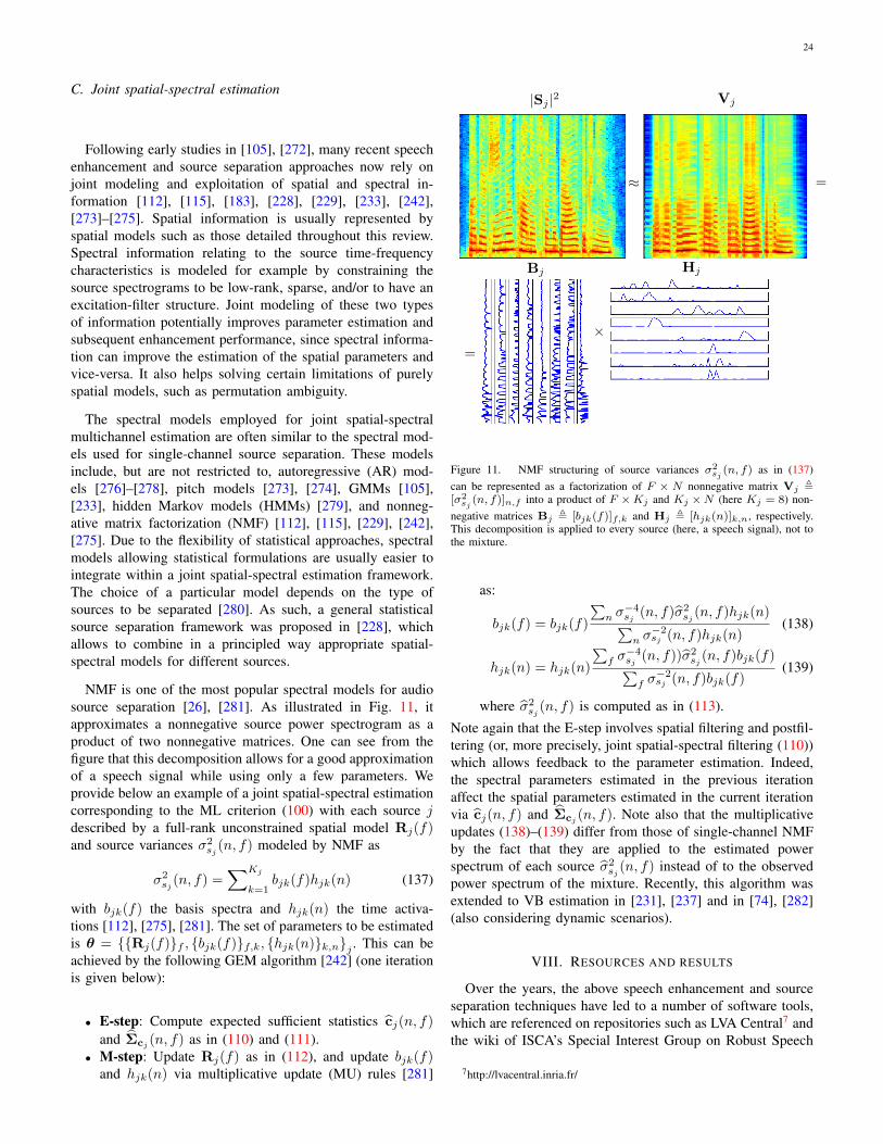
24

C. Joint spatial-spectral estimation

Following early studies in [105], [272], many recent speechenhancement and source separation approaches now rely onjoint modeling and exploitation of spatial and spectral in-formation [112], [115], [183], [228], [229], [233], [242],[273]–[275]. Spatial information is usually represented byspatial models such as those detailed throughout this review.Spectral information relating to the source time-frequencycharacteristics is modeled for example by constraining thesource spectrograms to be low-rank, sparse, and/or to have anexcitation-filter structure. Joint modeling of these two typesof information potentially improves parameter estimation andsubsequent enhancement performance, since spectral informa-tion can improve the estimation of the spatial parameters andvice-versa. It also helps solving certain limitations of purelyspatial models, such as permutation ambiguity.

The spectral models employed for joint spatial-spectralmultichannel estimation are often similar to the spectral mod-els used for single-channel source separation. These modelsinclude, but are not restricted to, autoregressive (AR) mod-els [276]–[278], pitch models [273], [274], GMMs [105],[233], hidden Markov models (HMMs) [279], and nonneg-ative matrix factorization (NMF) [112], [115], [229], [242],[275]. Due to the flexibility of statistical approaches, spectralmodels allowing statistical formulations are usually easier tointegrate within a joint spatial-spectral estimation framework.The choice of a particular model depends on the type ofsources to be separated [280]. As such, a general statisticalsource separation framework was proposed in [228], whichallows to combine in a principled way appropriate spatial-spectral models for different sources.

NMF is one of the most popular spectral models for audiosource separation [26], [281]. As illustrated in Fig. 11, itapproximates a nonnegative source power spectrogram as aproduct of two nonnegative matrices. One can see from thefigure that this decomposition allows for a good approximationof a speech signal while using only a few parameters. Weprovide below an example of a joint spatial-spectral estimationcorresponding to the ML criterion (100) with each source jdescribed by a full-rank unconstrained spatial model Rj(f)and source variances σ2

sj (n, f) modeled by NMF as

σ2sj (n, f) =

∑Kj

k=1bjk(f)hjk(n) (137)

with bjk(f) the basis spectra and hjk(n) the time activa-tions [112], [275], [281]. The set of parameters to be estimatedis θ = Rj(f)f , bjk(f)f,k, hjk(n)k,nj . This can beachieved by the following GEM algorithm [242] (one iterationis given below):

• E-step: Compute expected sufficient statistics cj(n, f)

and Σcj (n, f) as in (110) and (111).• M-step: Update Rj(f) as in (112), and update bjk(f)

and hjk(n) via multiplicative update (MU) rules [281]

Vj

≈

×

Bj Hj

|Sj |2

=

=

Figure 11. NMF structuring of source variances σ2sj

(n, f) as in (137)can be represented as a factorization of F × N nonnegative matrix Vj ,[σ2sj

(n, f)]n,f into a product of F ×Kj and Kj ×N (here Kj = 8) non-negative matrices Bj , [bjk(f)]f,k and Hj , [hjk(n)]k,n, respectively.This decomposition is applied to every source (here, a speech signal), not tothe mixture.

as:

bjk(f) = bjk(f)

∑n σ−4sj (n, f)σ2

sj (n, f)hjk(n)∑n σ−2sj (n, f)hjk(n)

(138)

hjk(n) = hjk(n)

∑f σ−4sj (n, f))σ2

sj (n, f)bjk(f)∑f σ−2sj (n, f)bjk(f)

(139)

where σ2sj (n, f) is computed as in (113).

Note again that the E-step involves spatial filtering and postfil-tering (or, more precisely, joint spatial-spectral filtering (110))which allows feedback to the parameter estimation. Indeed,the spectral parameters estimated in the previous iterationaffect the spatial parameters estimated in the current iterationvia cj(n, f) and Σcj (n, f). Note also that the multiplicativeupdates (138)–(139) differ from those of single-channel NMFby the fact that they are applied to the estimated powerspectrum of each source σ2

sj (n, f) instead of to the observedpower spectrum of the mixture. Recently, this algorithm wasextended to VB estimation in [231], [237] and in [74], [282](also considering dynamic scenarios).

VIII. RESOURCES AND RESULTS

Over the years, the above speech enhancement and sourceseparation techniques have led to a number of software tools,which are referenced on repositories such as LVA Central7 andthe wiki of ISCA’s Special Interest Group on Robust Speech

7http://lvacentral.inria.fr/

25

Table IISOME AIR DATASETS.

Name

#A

IRs

#m

icro

phon

es

#en

viro

nmen

ts

#m

ic.p

ositi

ons

#sp

eake

rpo

sitio

ns

inte

rpol

atio

npo

ssib

le

real

nois

e

RWCP [283]9 364 84 7 1 9 no noSiSEC [284]10 ∼50 2 5 1 ∼20 no noAIR [41]11 214 2 8 1 13 no noBinaural RIR [285]12 2920 8 5 1 365 yes yesCAMIL [266]13 32400 2 1 16200 1 yes noCHiME2 [286]14 242 2 1 1 121 yes yesRIRDB [287]15 1872 24 3 3 26 no no

Processing8. In the following, we provide a non-exhaustivelist of popular resources, databases and results, which will beuseful for readers to get an idea of the typical performancethat may be achieved and to start their own work in the field.

A. Datasets

A first approach to evaluation is to generate the test signalsby convolving clean speech signals with AIRs as in (3),summing them together as in (2), and possibly adding realrecorded noise. This makes it possible to control the sourcepositions and the room characteristics, which is useful in adevelopment stage. Table II lists a few AIR datasets. Each hasits own advantages, depending whether one is interested in avariety of environments, in a large number of microphones,in various speaker-microphone geometries, or in real noise.A variant of this approach which enables even more precisecontrol of the setup is to use artificial AIRs [288], [289]simulated using, e.g., Roomsim [290]16 or Room genera-tor17 and the respective spherical harmonic domain variantSMIRgen [291]18. Alternatively, one might record each sourceseparately and then sum all source images together [284],[292]. The series of Signal Separation Evaluation Campaigns(SiSEC) has shown that these three variants lead to comparableseparation quality [284]. Although they are often applied tonon-moving sources only, the generation of source movementsby AIR interpolation has recenty been justified in [286] and

8https://wiki.inria.fr/rosp/9http://research.nii.ac.jp/src/en/RWCP-SSD.html10https://sisec.inria.fr/11http://www.ind.rwth-aachen.de/de/forschung/tools-downloads/aachen-

impulse-response-database/12http://medi.uni-oldenburg.de/hrir/13https://team.inria.fr/perception/category/data/14http://spandh.dcs.shef.ac.uk/chime challenge/chime2013/15http://www.eng.biu.ac.il/˜gannot/RIR DATABASE16http://sourceforge.net/projects/roomsim/17http://www.audiolabs-erlangen.de/fau/professor/habets/software/rir-

generator18http://www.audiolabs-erlangen.de/fau/professor/habets/software/smir-

generator

Table IIISOME REAL MULTICHANNEL AUDIO DATASETS, FROM [293].

Name

scen

ario

dura

tion

(h)

#m

icro

phon

es

#en

viro

nmen

ts

spea

ker

dyna

mic

s

spea

ker

over

lap

Aurora-321 car ∼20 4 1 static noAMI [294]22 meeting 100 16 3 static yesDICIT [295]23 TV order 6 16 1 moving noCOSINE [296]24 discuss. 38 20 8 moving yesSWC [5]25 game 7 92 1 moving yesCHiME3 [297]26 tablet 19 6 4 moving babble

Table IVEVALUATION SOFTWARE.

Name Implemented metricsPESQ [299] perceptual speech quality (PESQ)PEMO-Q [300] perceptual similarity metric (PSM)STOI [301]27 short-time objective intelligibility (STOI)

Loizou’s [11]28

segmental signal-to-noise ratiolog-likelihood ratiocepstrum distancecomposite measure

BSS Eval [38]29signal-to-distortion ratio (SDR)signal-to-interference ratio (SIR)signal-to-artifacts ratio (SAR)

PEASS [302]30

overall perceptual score (OPS)target-related perceptual score (TPS)interference-rel. perceptual score (IPS)artifacts-related perceptual score (APS)

implemented in Roomsimove19 and Signal generator20.A second approach is to consider real recorded (and mixed)

signals. This is useful in a test stage, but it makes it harder toevaluate the results due to the fact that the true source signalsare unknown. Table III lists some datasets for which the targetspeakers have been recorded by a close-talk microphone so asto provide approximate ground truth. Once again, each datasethas its own advantages, depending whether one is interested ina particular use case, in the amount of data, in the number ofmicrophones, or in the presence of speech overlap. For moredetails and more datasets, see [293]. The use of mobile robotshas recently been proposed as a promising approach towardsrecording larger real datasets [298].

For either approach, the enhancement and separation qual-

19http://www.loria.fr/˜evincent/Roomsimove.zip20http://www.audiolabs-erlangen.de/fau/professor/habets/software/signal-

generator21http://catalog.elra.info/index.php?cPath=37 4022http://groups.inf.ed.ac.uk/ami/23http://shine.fbk.eu/resources/dicit-acoustic-woz-data24http://melodi.ee.washington.edu/cosine/25http://mini.dcs.shef.ac.uk/data-2/26http://spandh.dcs.shef.ac.uk/chime challenge/27http://amtoolbox.sourceforge.net/doc/speech/taal2011.php28http://www.crcpress.com/product/isbn/978146650421929http://bass-db.gforge.inria.fr/bss eval/30http://bass-db.gforge.inria.fr/peass/

26

ity can be evaluated by conducting subjective listeningtests [302]–[304] or by comparing the estimated source signalswith the true source signals using objective performancemetrics. Table IV lists a few metrics. According to the studyin [302], the frequency-weighted segmental SNR, the compos-ite metric in [11] and the OPS metric of PEASS [302] exhibitthe highest correlation with subjective assessment of overallquality.

B. Results

Some attempts were carried out to compare different sourceseparation methods e.g. [284], [305], beamforming methodse.g. [306], and source separation methods vs. beamformingmethods [307]. Most of the efforts were carried out in thesource separation research community, where six internationalSignal Separation Evaluation Campaigns (SiSEC) have beenrun since 2007 [284], [308]–[313]. This allows an objectivecomparison of different source separation approaches on thesame data. Moreover, several source separation methods wereused as pre-processing for speech recognition within a series ofspeech separation and recognition challenges [305]. It was alsoproposed to objectively evaluate the performance measuresof the corresponding source separation methods through theSiSEC campaigns [284].

As for beamforming methods, to the best of our knowledge,there is neither an evaluation campaign nor an evaluation papercomparing the performance of many different beamformerswith objective performance metrics. Some studies [306] eval-uate different beamformers as pre-processors for a speech rec-ognizer via speech recognition performance metrics. However,since the task used for this evaluation is different from theprimary goal of beamforming, it is difficult to conclude fromthese studies about the performance of the beamformers. Inthe coming years it is expected that an evaluation campaignwill become available in the beamforming community as well.Finally, the study in [307] compared some source separationmethods with some beamforming methods. These methods areevaluated for separation of one or two target speech sourcesfrom a diffuse background noise.

Hereafter we summarize some results from SiSEC cam-paigns that are relevant for this review. An overview andcomparative analysis of SASSEC [308], SiSEC 2008 [309]and SiSEC 2010 [310] can be found in [284]. Table V sum-marizes the results of five SiSEC campaigns for the “Under-determined speech and music mixtures” task over the samedataries that were reused from one campaign to another. TheSASSEC campaign [308] is not considered here, since it useda different dataset. We also excluded instantaneous mixtures(only convolutive mixtures are considered) since they are notrealistic, as well as music sources (only speech sources areconsidered) since they are out of the scope of this review.Finally, we excluded the results of partial source separationsubmissions, i.e. when the corresponding dataset was notprocessed entirely, since comparing such average results withothers is meaningless. As such, the figures in Table V do notcoincide in general with the figures from the correspondingSiSEC papers. Details about the considered dataries may be

found in the SiSEC papers and the corresponding web pages.We here, very briefly, recall their main characteristics (we usethe dataset names from the original campaigns):• test: synthetic or live recorded31 mixtures; 2 microphones

with 1 m or 5 cm spacing; 3 or 4 sources; 0.13 s or 0.25 sRT.

• test2: synthetic mixtures; 2 microphones with 20 cm or4 cm spacing; ; 3 or 4 sources; 0.13 s or 0.38 s RT.

• test3: synthetic mixtures; 3 microphones with 50 cm or5 cm spacing; 4 sources; 0.13 s or 0.38 s RT.

One can draw the following conclusions from the results inTable V. First, separating the live recorded mixtures does notseem to be more difficult than separating the synthetic ones.Second, the performance of the algorithms does not alwaysincrease from one campaign to another. This may be explainedby the fact that the participants do not usually resubmit themethod they have already tried in previous campaigns. Third,none of the methods can overcome the performance ceiling of5.5 dB SDR and 40 OPS. Finally, one can notice that the twoevaluation metrics may behave very differently (see, e.g. theresults of two submissions for SiSEC 2011 in Table V).

IX. SUMMARY AND PERSPECTIVES

This section concludes this survey article. First, we discussthe two major algorithmic families introduced in this survey,namely microphone array processing and BSS and their dif-ferences and similarities. Then, we provide some guidelineson the selection of the proper algorithm, based on the acousticscenario and available resources. We conclude this section andthe entire article by reviewing some current and future trendsin the field.

A. Microphone array processing and BSS: Differences andsimilarities

Two main paradigms for speech enhancement and sourceseparation were explored in this survey, namely microphonearray processing and BSS. We claim here that recent trendsare showing that these two paradigms are converging byborrowing ideas from each other.

Concerning the signal models, array processing methodstraditionally utilized the spatial resolution of the array as afunction of the DOA while BSS methods were originallydesigned for instantaneous mixtures (no delay, echoes orreverberation). It was then proposed, in the field of arrayprocessing, to substitute the simple DOA-based propagationmodel by ATFs and RTFs [66], [69]. In parallel, BSS methodsdeveloped from instantaneous mixtures to convolutive mix-tures also modeled by ATFs and RTFs [67], [321]. Under this

31For the synthetic mixtures the source images are artificially produced byconvolving the sources with the corresponding AIRs. For the live recordedmixtures the source images are physically recorded. In both cases the mixturesare produced synthetically by adding the corresponding source images.

32http://sisec2008.wiki.irisa.fr/33http://sisec2010.wiki.irisa.fr/34http://sisec2011.wiki.irisa.fr/35http://sisec2013.wiki.irisa.fr/36http://sisec.inria.fr/37The system is an extended version of the reference.

27

Table VSISEC 2008 - 2015 RESULTS FOR CONVOLUTIVE SPEECH MIXTURES OF “UNDER-DETERMINED SPEECH AND MUSIC MIXTURES” TASK. GRAY CELLSMEAN THAT EITHER THE DATASET OR THE EVALUATION METRIC WAS NOT CONSIDERED DURING THE CORRESPONDING EVALUATION CAMPAIGN, “-”

SIGN MEANS THAT THE CORRESPONDING DATASET WAS NOT PROCESSED ENTIRELY, AND THE HIGHEST SCORES ARE IN BOLD.

SiSEC Authors of submission MethodAverage of SDR metric [38] Average of OPS metric [302]

test test2 test3 test test2 test3Syn. Live Syn. Syn. Syn. Live Syn. Syn.

2008 [309]32Mandel [314] 1.14 1.91Weiss [315] 1.46 2.26El Chami [316] 3.02 2.95

2010 [310]33 Ozerov, Nesta and Vincent [228]37 1.77 2.66 1.72 21.2 37.9 26.8Sawada [317] 4.89 5.18 3.77 20.7 27.9 17.8

2011 [311]34

Cho [318] 3.09 2.54 1.19 26.6 26.3 29.7Nesta (1) [319]37 4.60 4.00 - 35.8 33.6 -Nesta (2) [319] 5.30 4.38 - 38.5 36.5 -Ozerov and Vincent [228]37 3.30 2.13 - 32.7 29.5 -Sawada [181] - - 5.28 - - 31.1

2013 [312]35 Cho [320] 5.29 4.69 5.24 31.1 30.5 34.75Adiloglu, Kayser and Wang [228], [231]37 2.70 0.75 3.23 30.0 23.3 35.22

2015 [313]36 Nguyen [181]37 5.06 4.01 4.27 36.2 32.6 35.55

perspective, there is no distinction between the two paradigmsanymore. As a matter of fact, their equivalence was alreadyobserved in an early stage [322].

Concerning the spatial filter design criteria, array processingtechniques traditionally rely on second-order statistics, whileBSS techniques can either apply second- or higher-orderstatistics. However, this distinction is not always applicable.In [323] higher-order statistics were utilized to estimate thesteering vectors of a beamformer. A structure, reminiscent ofthe GSC implementation, that utilizes higher-order statisticswas proposed in [324], where the signals are first separated byapplying a BSS method, then sorted according to their kurtosis,and finally the desired speech is further enhanced by means ofan adaptive noise canceller. More recently, information theo-retic criteria based on the TRINICON framework [184] wereincorporated into an LCMV beamformer [325]. Conversely,the most widely-used BSS methods today rely on second-orderstatistics, as popularized by [110]–[112], [227].

Geometry-based information (e.g. microphone distances andDOA) is usually exploited by array processing. It can howeveralso be incorporated into BSS criteria [70], [90], [326]. Theuse of priors [116], [182] breaks the “blindness” of BSS meth-ods even further. Conversely, some array processing methods,e.g. [69], [151], are not using any spatial priors but rather relyon a specific activity pattern.

Concerning the application of the methods, the array pro-cessing paradigm traditionally addressed speech detection,parameter estimation and signal separation successively, whilethe BSS paradigm addressed them in parallel. This line isbecoming blurred too, as certain BSS techniques relies on suc-cessive estimation [72], [85] while joint parameter estimationhas been used [276], [277] and is becoming more popular inthe array processing community [246], [247].

The scenario of several concurrently speaking speakersis well-studied in the BSS area, but more cumbersome inarray processing. It was shown in [137] (and extended laterin [95]), that the RTFs of the entire group of desired and

the entire group of interference sources can be estimated,provided that the group activities do not overlap during theestimation period. These RTFs estimators are then utilizedto construct a subspace-based LCMV beamformer. Recentcontributions [90], [327] circumvent the requirement for dis-joint activity of the desired and interference groups of sig-nals, by incorporating concepts from the BSS paradigm intothe beamformer design. Other array processing methods formultiple concurrent sources involve hypothesis testing for theactivity of the sources in T-F bins, before applying the optimalbeamformer [216], [233], [328].

Finally, classical beamformers do not handle under-determined problems. However, with the utilization of speechsparsity this becomes feasible for both paradigms [80], [150],[329].

We can therefore conclude that the array processing andBSS paradigms share many underling concepts, and willeventually converge to a point in which they will becomeindistinguishable.

B. Guidelines

We have surveyed a plethora of algorithms and methodsfor speech enhancement and separation. In this section wewill not attempt to pick up the “best” algorithm, but rathergive guidelines for selecting the most appropriate class ofalgorithms for a given scenario.

1) Number of sources and microphones: If there is only onesource in noise, the natural choice would be the MWF/MVDRfamily of beamformers. If multiple sources of interest exist(either desired or interference) but their number remainssmaller than the number of microphones, then LCMV beam-formers or BSS methods can be considered. If the number ofmicrophones is smaller than the number of sources of interest(under-determined problem), then the speech sparsity shouldbe utilized, usually in conjunction with BSS methods, but alsowith modern beamformers.

28

2) Array geometry: If the specific array geometry is known,e.g., linear, differential or spherical, preference should be givento array processing or source separation methods which exploitthis information. In entirely blind scenarios, BSS methodsare commonly used, however some modern array processingmethods based on ATFs or RTFs can also be used.

3) Prior information: If additional prior information isavailable, preference should be given to methods which exploitthis information. For instance, information about the sourceDOA can be exploited both by array processing and sourceseparation methods, while information about the nature of thesources and training data is more easily exploited by the latter.

C. Perspectives

In this section we explore some of the current and futuretrends in the field of multi-microphone array processing.

1) Learning-based spatial filters: The signal models wehave reviewed in this article rely on limited prior information:the ATFs (or the respective RTFs) are assumed to be eitherunconstrained, or to satisfy universal constraints dependingon the source positions [70], [81] and the room reverberationtime [61], [116]. What if the exact shape and acoustic proper-ties of the room were fixed? In this situation, one would knowthe exact ATFs/RTFs associated with all possible source andmicrophone positions. Source localization and ATF estimationwould become identical problems, that would be much easierto solve. This ideal situation can be approximated in practiceby acquiring ATFs for a finite set of source and microphonepositions using mobile devices and interpolating them to findthe ATFs in other positions, using the fact that the set ofATFs in a given room forms a (nonlinear) manifold. Thisidea has recently been the starting point for an increasingnumber of studies which model the manifold of ATFs usingmodels based on sparsity and compressed sensing [56], [57],[60], [330]–[334] or locally linear embedding and manifoldlearning [62], [335]–[338]. A preliminary study of applyingthe latter concepts to construct a GSC beamformer can befound in [339]. Extending these approaches to work across afull, real-world room is an exciting perspective.

2) Deep learning-based parameter estimation: deep neuralnetworks (DNNs) have emerged as a promising alternativeto SPP estimation, EM, VB, or MM in the situations whenlarge amounts (typically, hours) of source signals similar tothose in the mixture to be separated, are available for training.DNNs model complex, high-dimensional functions by makingefficient use of this wealth of data. They typically operatein the magnitude STFT domain, take several frames of themixture as inputs, and output the SPP or the spectra of allsources in each time frame. Most work in this area has focusedand still focuses on single-channel separation using spectralcues or channel-wise filtering using ILD and ITD cues [340]or pitch and azimuth [341] (using multi-layer perceptrons).

Yet, a few multichannel approaches have recently beenproposed that use DNNs in a variety of ways: to estimatethe SPP using a DNN and subsequently derive a beam-former [342], to alternately reestimate the source magnitudespectra using DNNs and the spatial covariance matrices in

an EM-like fashion [343], or to learn beamformers directlyin the time domain [344]. The integration of these data-driven techniques with the domain knowledge learned fromthe established techniques presented in this review is an openresearch direction.

3) Distributed algorithms for ad hoc microphone arrays:In classical microphone array processing, as explored in thissurvey, both the sensing and the processing of the acquiredspeech are concentrated in a single device, usually calleda fusion center. In many scenarios, this approach cannotprovide the required performance, since the acoustic scenemay be spatially distributed, and a powerful fusion centermay not be available. It is therefore reasonable to allevi-ate the performance drop by a large spatial deployment ofinter-connected microphone sub-arrays (nodes), arranged in awireless network, preferably equipped with local processors.Recent technological advances in the design of miniature andlow-power electronic devices make such distributed micro-phone networks, often referred to as wireless acoustic sensornetwork (WASN), feasible. As a matter of fact, cellular phone,laptops and tablets are perfect candidates as nodes of suchnetworks, as they are self-powered and equipped with multiplemicrophones (typically two to three), as well as powerfulprocessors and various wireless communication modules. Thelarge spatial distribution of WASNs increases the probabilitythat a subset of the microphones is close to a relevant soundsource and has the potential to yield improved performanceas compared with classical, condensed, microphone arrays.However, the distributed and ad hoc nature of WASNs arisesnew challenges, e.g. transmission and processing constraintsand intricate network topology, that should be addressed tofully exploit their potential.

Several families of algorithms, that allow for optimal solu-tions without requiring the transmission of all signals to a cen-tral processor, but rather a compressed/fused version thereof,have been proposed [345]. One such family is the distributedadaptive node-specific signal estimation (DANSE) family ofalgorithms, which allow for a distributed implementation ofseveral speech enhancement algorithms that were introducedin this survey (including SDW-MWF [346], [347] and LCMVbeamforming [220]). Several network topologies can be im-plemented, e.g. fully-connected and tree-structure. Anotherfamily of algorithms exploits the special GSC structure toobtain recursive solutions that are proven to converge to theoptimal beamforming criteria [348]. Theoretical performancebounds of such distributed microphone array algorithms canbe derived [349]. Efficient adaptation mechanisms to changesin the number of available nodes and signals of interest canbe found in [350].

Randomized gossip implementation of the DS beamformeris presented in [351]. A distributed algorithm for MVDRbeamforming, based on message passing, is presented in [352].A distributed MVDR beamformer based on the diffusionadaptation paradigm, that neither imposes conditions on thetopology of the network nor requires knowledge of the noisecovariance matrix, can be found in [353]. Near-field beam-formers using smartphones forming an ad hoc network aredescribed in [354]. Intra- and inter-node location features are

29

integrated in a clustering-based scheme for speech separationin [355].

In practical scenarios the microphone signals can have anarbitrary temporal offsets. A method to alleviate this problemcan be found in [356]. In severe cases, identical samplingfrequency across all nodes cannot be guaranteed. Method tore-synchronize the signals, either based on the communicationlink, on the speech signals, or on a combination thereof, canbe found in [357]–[365].

Despite these advances in the field of distributed algorithmsfor ad hoc microphone arrays, the quest for a full-fledgedsolution, considering all challenges in reverberant and dynamicacoustic environment, is still far from reached.

4) Robustness: Two kinds of robustness can be attributedto beamformers, namely numerical robustness and spatialrobustness [366]. Numerical robustness refers to the sensitivityof the array gain to mismatches in the microphone gainsand phases and the beamformer weights. As was alreadyexplored in Section IV-A in the general context of (narrow-band) array processing, numerical robustness is proportionalto the WNG [118], [121] (see modification for structuredarrays in [122]). It is further proposed in [121] to increasethe robustness, trading-off array directivity, using diagonalloading. In [367] it is proposed to increase the robustness of abroadband array with an arbitrary directivity, by incorporatingthe probability density functions of the microphone gains andphases into the beamformer design criterion. The statistics ofthe microphone characteristics is also taken into account in thedesign of a robust superdirective beamformer (e.g. differentialmicrophone arrays) [368].

The term spatial robustness refers to mismatches betweenthe actual location of a desired source and the assumedlocation used to derive the beamformer weights. It is awidely-explored area in the field of array processing [369]–[371]. Widening the beampattern is a common practice toincrease robustness to steering errors. This can be done byeither adding derivative constraints [189], by methods bor-rowed from filtering design procedures [372], or by definingmultiple constraints in an area surrounding the prospectivesource location [191]. Alternatively, a probabilistic frameworkfor describing the errors in the steering vectors is proposedin [366] to design a robust beamformer based on the maximumsignal to interference plus noise ratio (SINR) criterion.

The GSC structure is utilized to combine spatial robust-ness considerations (in the BM block) and numerical robust-ness considerations (in the adaptive noise canceller (ANC)block) [199], [200]. A GSC-type beamformer utilizing ad-vanced BSS techniques, namely TRINICON, is also proposedfor increasing robustness [373].

Although many methods for increasing the robustness ofbeamformers in speech applications can be found in theliterature, designing a robust beamformer that takes roomacoustics and speech properties into account, remains an openresearch question.

5) Dynamic scenarios and tracking: The application ofbeamforming and BSS techniques, explored in this survey,to dynamic scenarios is a cumbersome task, mainly due tothe limited amount of data available for estimating the time-

varying filters. Methods that utilizes instantaneous direction-of-arrival estimates to allow for fast adaptation of LCMVbeamformers can be found in [163], [374]. A tracking mech-anism for the RTFs of the desired and interference sources,based on subspace tracking [375], is described in [198]. Thetime-varying estimates of the RTF are utilized to designLCMV beamformer to extract the set of desired speakers.EM and VB frameworks were also proposed in [74], [114],[282]. The resulting algorithms employ a Kalman smootherto estimate time-varying mixing filters, that are subsequentlyutilized to construct Wiener filters for separating the sourcesin under-determined mixtures.

6) Binaural multi-microphone processing: The objective ofa binaural noise reduction algorithm is not only to selectivelyextract the desired speaker and to suppress interfering sourcesand ambient background noise, but also to preserve the audi-tory impression, as perceived by the hearing aid user. Existingmethods can be roughly categorized into three main families.

The first family is based on the concept of CASA [376]–[378], which aims at imitating the behavior of the humanauditory system [25], [379].

The second family consists of BSS algorithms [380]–[382],which are based on the fundamental assumption of mutualstatistical independence of the different source signals.

The third family is based on a binaural versions of theMMSE [92], MVDR and LCMV criteria. The binaural MWFinherently preserves the binaural cues of the desired source butdistorts the binaural cues of the noise (i.e. the beamformer im-poses the noise to be coherent and perceived as arriving fromthe same direction as the desired source). Several extensionsof the binaural MWF have been introduced aiming to alsopreserve the binaural cues of the noise [93], [96], [97], [383].By design, these methods suffer from some distortion imposedon the desired source component at the output. Alternatively,distortionless criteria, such as the MVDR and LCMV, can beused instead of MWF [95], [98], [384]–[386].

Hearing aids impose severe design constraints on the devel-oped algorithm: short latency, fast adaption, small number ofmicrophones, limited connectivity between the hearing devicesand low-complexity, to name a few. Designing algorithms,satisfying these constraints, and still exhibiting high noise andinterference reduction together spatial cues preservation, is stillan ongoing research topic.

7) Audio-visual speech enhancement: Finally, although wehave focused on audio-only algorithms above, one must bearin mind that microphones are quite often embedded in devicesequipped with other sensors, e.g., cameras, accelerometers.In [387], cameras have been used to estimate speech statisticsfrom visual (face and lips) features and noise statistics fromvisual voice activity detection. They have also been usedto find the spatial location of the sources in [388]–[391].An optimal integration of acoustic and visual information isobtained by joint inference in both modalities using the turbo-decoding framework [392]. In [393] an audio-visual voiceactivity detection is proposed, using dimensionality reduction.

The area of audio-visual speech processing remains largelyunderstudied despite its great promise.

30

REFERENCES

[1] A. Boothroyd, K. Fitz, J. Kindred, S. Kochkin, H. Levitt, B. Moore,and J. Yanz, “Hearing aids and wireless technology,” Hearing Review,vol. 14, no. 6, pp. 44, 2007.

[2] J. Flanagan, J. Johnston, R. Zahn, and G. Elko, “Computer-steeredmicrophone arrays for sound transduction in large rooms,” J. Acoust.Soc. of Am., vol. 78, no. 5, pp. 1508–1518, 1985.

[3] H. Silverman, I. Patterson, W.R., J. Flanagan, and D. Rabinkin, “Adigital processing system for source location and sound capture bylarge microphone arrays,” in Acoustics, Speech, and Signal Processing,1997. ICASSP-97., 1997 IEEE International Conference on, Apr. 1997,vol. 1, pp. 251–254.

[4] D. Mostefa, N. Moreau, K. Choukri, G. Potamianos, S. Chu, et al.,“The CHIL audiovisual corpus for lecture and meeting analysis insidesmart rooms,” Lang. Resources Eval., vol. 41, no. 3–4, pp. 389–407,2007.

[5] C. Fox, Y. Liu, E. Zwyssig, and T. Hain, “The Sheffield wargamescorpus,” in Proc. Interspeech, 2013, pp. 1116–1120.

[6] L. Cristoforetti, M. Ravanelli, M. Omologo, A. Sosi, A. Abad, M. Hag-mueller, and P. Maragos, “The DIRHA simulated corpus,” in Proc.Int. Conf. on Lang. Res. and Eval., 2014.

[7] E. Vincent, R. Gribonval, and M. D. Plumbley, “Oracle estimators forthe benchmarking of source separation algorithms,” Sig. Proc., vol. 87,no. 8, pp. 1933–1950, 2007.

[8] S. L. Gay and J. Benesty, Eds., Acoustic signal processing fortelecommunication, Kluwer, 2000.

[9] M. S. Brandstein and D. B. Ward, Eds., Microphone Arrays: SignalProcessing Techniques and Applications, Springer, 2001.

[10] J. Benesty, S. Makino, and J. Chen, Eds., Speech Enhancement,Springer, 2005.

[11] P. C. Loizou, Speech Enhancement: Theory and Practice, CRC Press,2007.

[12] I. Cohen, J. Benesty, and S. Gannot, Eds., Speech processing in moderncommunication: Challenges and perspectives, Springer, 2010.

[13] P. O’Grady, B. Pearlmutter, and S. T. Rickard, “Survey of sparse andnon-sparse methods in source separation,” Int. J. Imag. Sys. Tech., vol.15, pp. 18–33, 2005.

[14] S. Makino, T.-W. Lee, and H. Sawada, Eds., Blind speech separation,Springer, 2007.

[15] M. S. Pedersen, J. Larsen, U. Kjems, and L. C. Parra, “Convolutiveblind source separation methods,” in Springer Handbook of SpeechProcessing, pp. 1065–1094. Springer, 2008.

[16] P. Comon and C. Jutten, Eds., Handbook of Blind Source Separation,Independent Component Analysis and Applications, Academic Press,2010.

[17] E. Vincent, M. Jafari, S. A. Abdallah, M. D. Plumbley, and M. E.Davies, “Probabilistic modeling paradigms for audio source separa-tion,” in Machine Audition: Principles, Algorithms and Systems, pp.162–185. IGI Global, 2010.

[18] E. Vincent, N. Bertin, R. Gribonval, and F. Bimbot, “From blind toguided audio source separation: How models and side information canimprove the separation of sound,” IEEE Sig. Proc. Mag., vol. 31, no.3, pp. 107–115, 2014.

[19] U. Zolzer, Ed., DAFX: Digital Audio Effects, Wiley, 2011.[20] A. Ozerov, C. Fevotte, R. Blouet, and J.-L. Durrieu, “Multichannel

nonnegative tensor factorization with structured constraints for user-guided audio source separation,” in Proc. IEEE Intl. Conf. on Acous.,Sp. and Sig. Proc. (ICASSP), Prague, May 2011, pp. 257–260.

[21] N. Sturmel, A. Liutkus, J. Pinel, L. Girin, S. Marchand, G. Richard,R. Badeau, and L. Daudet, “Linear mixing models for active listeningof music productions in realistic studio conditions,” in Proc. Au. Eng.Soc. Conv., 2012.

[22] E. Hansler and G. Schmidt, Acoustic Echo and Noise Control: Apractical Approach, Wiley, 2004.

[23] P. A. Naylor and N. D. Gaubitch, Eds., Speech Dereverberation,Springer, 2010.

[24] P. Divenyi, Ed., Speech Separation by Humans and Machines, SpringerVerlag, 2004.

[25] D. Wang and G. J. Brown, Eds., Computational Auditory SceneAnalysis: Principles, Algorithms, and Applications, Wiley, 2006.

[26] T. Virtanen, J. F. Gemmeke, B. Raj, and P. Smaragdis, “Compositionalmodels for audio processing,” IEEE Sig. Proc. Mag., vol. 32, no. 2,pp. 125–144, 2015.

[27] I. Cohen and S. Gannot, “Spectral enhancement methods,” in SpringerHandbook of Speech Processing and Speech Communication. Springer,2007.

[28] M. Wolfel and J. McDonough, Distant Speech Recognition, Wiley,2009.

[29] T. Virtanen, R. Singh, and B. Raj, Eds., Techniques for NoiseRobustness in Automatic Speech Recognition, Wiley, 2012.

[30] J. Li, L. Deng, Y. Gong, and R. Haeb-Umbach, “An overview of noise-robust automatic speech recognition,” IEEE/ACM Trans. Au., Sp., Lang.Proc., vol. 22, no. 4, pp. 745–777, 2014.

[31] N. Ono, K. Miyamoto, H. Kameoka, J. Le Roux, Y. Uchiyama,E. Tsunoo, T. Nishimoto, and S. Sagayama, “Harmonic and percussivesound separation and its application to MIR-related tasks,” in Advancesin Music Information Retrieval. Springer, 2010.

[32] C. Knapp and G. Carter, “The generalized correlation method forestimation of time delay,” IEEE Trans. Acoust., Sp., Sig. Proc., vol.24, no. 4, pp. 320–327, 1976.

[33] J. Chen, J. Benesty, and Y. Huang, “Time delay estimation in roomacoustic environments: an overview,” EURASIP J. on Appl. Sig. Proc.,vol. 2006, pp. 1–19, 2006.

[34] A. Brutti, M. Omologo, and P. Svaizer, “Comparison between differentsound source localization techniques based on a real data collection,”in Proc. Joint Workshop on Hands-free Sp. Comm. and Mic. Arrays.IEEE, 2008, pp. 69–72.

[35] H. Kuttruff, Room acoustics, Taylor & Francis, 2000.[36] J. Blauert, Spatial Hearing: The Psychophysics of Human Sound

Localization, MIT Press, 1997.[37] D. Markovic, K. Kowalczyk, F. Antonacci, C. Hofmann, A. Sarti, and

W. Kellermann, “Estimation of acoustic reflection coefficients throughpseudospectrum matching,” IEEE/ACM Trans. Au., Sp., Lang. Proc.,vol. 22, no. 1, pp. 125–137, Jan. 2014.

[38] E. Vincent, R. Gribonval, and C. Fevotte, “Performance measurementin blind audio source separation,” IEEE Trans. Au., Sp., Lang. Proc.,vol. 14, no. 4, pp. 1462–1469, 2006.

[39] J.-F. Cardoso, “Multidimensional independent component analysis,” inProc. IEEE Intl. Conf. on Acous., Sp. and Sig. Proc. (ICASSP), 1998,vol. 4, pp. 1941–1944.

[40] S.-K. Lee, “Measurement of reverberation times using a wavelet filterbank and application to a passenger car,” Journal Au. Eng. Soc., vol.52, no. 5, pp. 506–515, 2004.

[41] M. Jeub, M. Schafer, and P. Vary, “A binaural room impulse responsedatabase for the evaluation of dereverberation algorithms,” in Proc.IEEE Int. Conf. on Dig. Sig. Proc., 2009, pp. 1–4.

[42] M. R. Schroeder, “Statistical parameters of the frequency responsecurves of large rooms,” Journal Au. Eng. Soc., vol. 35, no. 5, pp.299–306, 1987.

[43] J.-D. Polack, “Playing billiards in the concert hall: The mathematicalfoundations of geometrical room acoustics,” Appl. Acous., vol. 38, no.2, pp. 235–244, 1993.

[44] M. R. Schroeder, “Frequency correlation functions of frequencyresponses in rooms,” J. Acoust. Soc. of Am., vol. 34, no. 12, pp. 1819–1823, 1963.

[45] T. Gustafsson, B. D. Rao, and M. Trivedi, “Source localization inreverberant environments: Modeling and statistical analysis,” IEEETrans. Sp. Au. Proc., vol. 11, pp. 791–803, 2003.

[46] R. Scharrer and M. Vorlander, “Sound field classification in smallmicrophone arrays using spatial coherences,” IEEE Trans. Au., Sp.,Lang. Proc., vol. 21, no. 9, pp. 1891–1899, Sept. 2013.

[47] O. Schwartz, E. Habets, and S. Gannot, “Nested generalized sidelobecanceller for joint dereverberation and noise reduction,” in Proc. IEEEIntl. Conf. on Acous., Sp. and Sig. Proc. (ICASSP), Brisbane, Australia,Apr. 2015.

[48] H.-L. Nguyen Thi and C. Jutten, “Blind source separation forconvolutive mixtures,” Sig. Proc., vol. 45, no. 2, pp. 209–229, 1995.

[49] S. Choi and A. Cichocki, “Adaptive blind separation of speech signals:Cocktail party problem,” in Proc. IEEE Int. Conf. on Sig. Proc., 1997,pp. 617–622.

[50] F. Ehlers and H. G. Schuster, “Blind separation of convolutivemixtures and an application in automatic speech recognition in a noisyenvironment,” IEEE Trans. Sig. Proc., vol. 45, no. 10, pp. 2608–2612,1997.

[51] R. H. Lambert and A. J. Bell, “Blind separation of multiple speakersin a multipath environment,” in Proc. IEEE Intl. Conf. on Acous., Sp.and Sig. Proc. (ICASSP), 1997, pp. I–423–I–426.

[52] H.-C. Wu and J. C. Prıncipe, “Generalized anti-Hebbian learning forsource separation,” in Proc. IEEE Intl. Conf. on Acous., Sp. and Sig.Proc. (ICASSP), 1999, pp. II–1073–II–1076.

31

[53] M. Ito, Y. Takeuchi, T. Matsumoto, H. Kudo, M. Kawamoto, T. Mukai,and N. Ohnishi, “Moving-source separation using directional micro-phones,” in Proc. Intl. Symp. on Sig. Proc. and Info. Tech. (ISSPIT),2002, pp. 523–526.

[54] A. Aissa-El-Bey, K. Abed-Meraim, and Y. Grenier, “Blind separationof underdetermined convolutive mixtures using their time-frequencyrepresentation,” IEEE Trans. Au., Sp., Lang. Proc., vol. 15, no. 5, pp.1540–1550, 2007.

[55] M. Gupta and S. C. Douglas, “Beamforming initialization and dataprewhitening in natural gradient convolutive blind source separationof speech mixtures,” in Proc. Int. Conf. on Independent ComponentAnalysis and Blind Signal Separation (ICA), 2007, pp. 462–470.

[56] Y. Lin, J. Chen, Y. Kim, and D. D. Lee, “Blind channel identificationfor speech dereverberation using `1-norm sparse learning,” in Proc.Neural Info. Proc. Conf., 2007, pp. 921–928.

[57] P. Sudhakar, S. Arberet, and R. Gribonval, “Double sparsity: Towardsblind estimation of multiple channels,” in Proc. Int. Conf. on LatentVariable Analysis and Signal Separation (LVA/ICA), 2010, pp. 571–578.

[58] M. Yu, W. Ma, J. Xin, and S. Osher, “Multi-channel `1 regularizedconvex speech enhancement model and fast computation by the splitbregman method,” IEEE Trans. Au., Sp., Lang. Proc., vol. 20, no. 2,pp. 661–675, 2012.

[59] I. J. Kelly and F. M. Boland, “Detecting arrivals in room impulseresponses with dynamic time warping,” IEEE/ACM Trans. Au., Sp.,Lang. Proc., vol. 22, no. 7, pp. 1139–1147, July 2014.

[60] Z. Koldovky, J. Malek, and S. Gannot, “Spatial source subtractionbased on incomplete measurements of relative transfer function,”IEEE/ACM Transactions on Audio, Speech, and Language Processing,pp. 1335–1347, Aug. 2015.

[61] A. Benichoux, L. S. R. Simon, E. Vincent, and R. Gribonval, “Con-vex regularizations for the simultaneous recording of room impulseresponses,” IEEE Trans. Sig. Proc., vol. 62, no. 8, pp. 1976–1986,Apr. 2014.

[62] B. Laufer, R. Talmon, and S. Gannot, “A study on manifolds of acousticresponses,” in Latent Variable Analysis and Independent ComponentAnalysis (LVA-ICA), Liberec, Czech Republic, Aug. 2015.

[63] M. Kowalski, E. Vincent, and R. Gribonval, “Beyond the narrowbandapproximation: Wideband convex methods for under-determined rever-berant audio source separation,” IEEE Trans. Au., Sp., Lang. Proc.,vol. 18, no. 7, pp. 1818–1829, 2010.

[64] J. Chen, J. Benesty, and Y. Huang, “A minimum distortion noisereduction algorithm with multiple microphones,” IEEE Trans. Au.,Sp., Lang. Proc., vol. 16, no. 3, pp. 481–493, 2008.

[65] R. Crochiere and L. Rabiner, Multi-Rate Signal Processing, EnglewoodCliffs, NJ: Prentice Hall, 1983.

[66] S. Affes and Y. Grenier, “A signal subspace tracking algorithm formicrophone array processing of speech,” IEEE Trans. Sp. Au. Proc.,vol. 5, no. 5, pp. 425–437, Sept. 1997.

[67] P. Smaragdis, “Blind separation of convolved mixtures in the frequencydomain,” Neurocomputing, vol. 22, pp. 21–34, 1998.

[68] S. Ikeda and N. Murata, “An approach to blind source separationof speech signals,” in Proc. Int. Conf. on Artificial Neural Networks(ICANN), 1998, pp. 761–766.

[69] S. Gannot, D. Burshtein, and E. Weinstein, “Signal enhancement usingbeamforming and nonstationarity with applications to speech,” IEEETrans. Sig. Proc., vol. 49, no. 8, pp. 1614–1626, Aug. 2001.

[70] L. C. Parra and C. V. Alvino, “Geometric source separation: Mergingconvolutive source separation with geometric beamforming,” IEEETrans. Sp. Au. Proc., vol. 10, no. 6, pp. 352–362, Sept. 2002.

[71] B. Albouy and Y. Deville, “Alternative structures and power spectrumcriteria for blind segmentation and separation of convolutive speechmixtures,” in Proc. Int. Conf. on Independent Component Analysisand Blind Signal Separation (ICA), 2003, pp. 361–366.

[72] S. Winter, H. Sawada, S. Araki, and S. Makino, “Overcomplete BSSfor convolutive mixtures based on hierarchical clustering,” in Proc. Int.Conf. on Independent Component Analysis and Blind Signal Separation(ICA), 2004, pp. 652–660.

[73] S. Araki, R. Mukai, S. Makino, T. Nishikawa, and H. Saruwatari, “Thefundamental limitation of frequency domain blind source separation forconvolutive mixtures of speech,” IEEE Trans. Sp. Au. Proc., vol. 11,no. 2, pp. 109–116, Mar. 2003.

[74] D. Kounades-Bastian, L. Girin, X. Alameda-Pineda, S. Gannot, andR. P. Horaud, “A variational EM algorithm for the separation of movingsound sources,” in Proc. IEEE Workshop on App. of Sig. Proc. to Au.and Acous. (WASPAA), New Paltz, USA, Oct. 2015.

[75] H. Sawada, R. Mukai, S. F. G. M. de la Kethulle de Ryhove, S. Araki,and S. Makino, “Spectral smoothing for frequency-domain blind sourceseparation,” in Proc. Intl. Workshop Acoust. Echo Noise Control(IWAENC), 2003, pp. 311–314.

[76] F. N. ans P. Svaizer and M. Omologo, “Convolutive BSS of shortmixtures by ICA recursively regularized across frequencies,” IEEETrans. Au., Sp., Lang. Proc., vol. 19, no. 3, pp. 624–639, 2011.

[77] M. Knaak, S. Araki, and S. Makino, “Geometrically constrainedindependent component analysis,” IEEE Trans. Au., Sp., Lang. Proc.,vol. 15, no. 2, pp. 715–726, 2007.

[78] K. Reindl, Y. Zheng, A. Schwarz, S. Meier, R. Maas, A. Sehr, andW. Kellermann, “A stereophonic acoustic signal extraction scheme fornoisy and reverberant environments,” Comp. Sp. and Lang., vol. 27,no. 3, pp. 726–745, 2013.

[79] S. Leglaive, R. Badeau, and G. Richard, “Multichannel audio sourceseparation with probabilistic reverberation modeling,” in Proc. IEEEWorkshop on App. of Sig. Proc. to Au. and Acous. (WASPAA), NewPaltz, NY, United States, Oct. 2015.

[80] S. Araki, H. Sawada, R. Mukai, and S. Makino, “Underdeterminedblind sparse source separation for arbitrarily arranged multiple sensors,”Sig. Proc., vol. 87, no. 8, pp. 1833–1847, Aug. 2007.

[81] H. Sawada, S. Araki, R. Mukai, and S. Makino, “Grouping separatedfrequency components with estimating propagation model parametersin frequency-domain blind source separation,” IEEE Trans. Au., Sp.,Lang. Proc., vol. 15, no. 5, pp. 1592–1604, 2007.

[82] S. Stenzel, J. Freudenberger, and G. Schmidt, “A minimum variancebeamformer for spatially distributed microphones using a soft referenceselection,” in Proc. Joint Workshop on Hands-free Sp. Comm. and Mic.Arrays, May 2014, pp. 127–131.

[83] A. Deleforge, S. Gannot, and W. Kellermann, “Towards a generaliza-tion of relative transfer functions to more than one source,” in Proc.European Sig. Proc. Conf. (EUSIPCO), 2015, pp. 419–423.

[84] X. Li, R. Horaud, L. Girin, and S. Gannot, “Local relative transferfunction for sound source localization,” in Proc. European Sig. Proc.Conf. (EUSIPCO), 2015, pp. 399–403.

[85] O. Yılmaz and S. T. Rickard, “Blind separation of speech mixtures viatime-frequency masking,” IEEE Trans. Sig. Proc., vol. 52, no. 7, pp.1830–1847, 2004.

[86] M. Puigt and Y. Deville, “Time-frequency ratio-based blind separationmethods for attenuated and time-delayed sources,” Mech. Syst. SignalProcess, vol. 19, pp. 1348–1379, 2005.

[87] T. Melia and S. T. Rickard, “Underdetermined blind source separationin echoic environments using DESPRIT,” EURASIP J. on Adv. in Sig.Proc., vol. 2007, pp. 1–19, 2007.

[88] C. Liu, B. C. Wheeler, W. D. O’Brien Jr., C. R. Lansing, R. C. Bilger,D. L. Jones, and A. S. Feng, “A two-microphone dual delay-lineapproach for extraction of a speech sound in the presence of multipleinterferers,” J. Acoust. Soc. of Am., vol. 110, no. 6, pp. 3218–3231,Dec. 2001.

[89] J. Anemuller and B. Kollmeier, “Adaptive separation of acousticsources for anechoic conditions: A constrained frequency domainapproach,” Sp. Comm., vol. 39, no. 1–2, pp. 79–95, 2003.

[90] K. Reindl, S. Markovich-Golan, H. Barfuss, S. Gannot, and W. Keller-mann, “Geometrically constrained TRINICON-based relative transferfunction estimation in underdetermined scenarios,” in Proc. IEEEWorkshop on App. of Sig. Proc. to Au. and Acous. (WASPAA), NewPaltz, USA, Oct. 2013.

[91] A. Bronkhorst and R. Plomp, “The effect of head-induced interauraltime and level differences on speech intelligibility in noise,” J. Acoust.Soc. of Am., vol. 83, no. 4, pp. 1508–1516, 1988.

[92] S. Doclo, S. Gannot, M. Moonen, and A. Spriet, “Acoustic beamform-ing for hearing aid applications,” in Handbook on Array Processingand Sensor Networks, S. Haykin and K. Liu, Eds. Wiley-IEEE Press,2010.

[93] B. Cornelis, S. Doclo, T. Van dan Bogaert, M. Moonen, and J. Wouters,“Theoretical analysis of binaural multimicrophone noise reductiontechniques,” IEEE Trans. Au., Sp., Lang. Proc., vol. 18, no. 2, pp.342–355, 2010.

[94] D. Marquardt, V. Hohmann, and S. Doclo, “Coherence preservationin multi-channel wiener filtering based noise reduction for binauralhearing aids,” in Proc. IEEE Intl. Conf. on Acous., Sp. and Sig. Proc.(ICASSP), 2013, pp. 8648–8652.

[95] E. Hadad, S. Gannot, and S. Doclo, “Binaural linearly constrainedminimum variance beamformer for hearing aid applications,” in Proc.Intl. Workshop Acoust. Sig. Enh. (IWAENC), Aachen, Germany, Sept.2012.

32

[96] D. Marquardt, E. Hadad, S. Gannot, and S. Doclo, “Theoretical analysisof linearly constrained multi-channel Wiener filtering algorithms forcombined noise reduction and binaural cue preservation in binauralhearing aids,” IEEE/ACM Trans. Au., Sp., Lang. Proc., pp. 2384–2397,Dec. 2015.

[97] D. Marquardt, V. Hohmann, and S. Doclo, “Interaural coherencepreservation in multi-channel Wiener filtering-based noise reductionfor binaural hearing aids,” IEEE/ACM Trans. Au., Sp., Lang. Proc.,vol. 23, no. 12, pp. 2162–2176, Dec. 2015.

[98] E. Hadad, D. Marquardt, S. Doclo, and S. Gannot, “Theoretical analysisof binaural transfer function MVDR beamformers with interference cuepreservation constraints,” IEEE/ACM Trans. Au., Sp., Lang. Proc., pp.2449–2464, Dec. 2015.

[99] E. Hadad, S. Doclo, and S. Gannot, “The binaural LCMV beamformerand its performance analysis,” IEEE/ACM Trans. Au., Sp., Lang. Proc.,vol. 24, no. 3, pp. 543–558, Mar. 2016.

[100] J. Shynk, “Frequency-domain and multirate and adaptive filtering,”IEEE Sig. Proc. Mag., vol. 9, no. 1, pp. 14–37, Jan. 1992.

[101] M. R. Portnoff, “Time-frequency representation of digital signals andsystems based on short-time Fourier analysis,” IEEE Trans. Acoust.,Sp., Sig. Proc., vol. 28, no. 1, pp. 55–69, Feb. 1980.

[102] J. Le Roux and E. Vincent, “Consistent Wiener filtering for audiosource separation,” IEEE Signal Process. Lett., vol. 20, no. 3, pp.217–220, 2013.

[103] A. Gilloire and M. Vetterli, “Adaptive filtering in subbands withcritical sampling: analysis, experiments, and application to acousticecho cancellation,” IEEE Trans. Sig. Proc., vol. 40, no. 8, pp. 1862–1875, Aug. 1992.

[104] Y. Avargel and I. Cohen, “Adaptive system identification in theshort-time fourier transform domain using cross-multiplicative transferfunction approximation,” IEEE Trans. Au., Sp., Lang. Proc., vol. 16,no. 1, pp. 162–173, Jan. 2008.

[105] H. Attias, “New EM algorithms for source separation and deconvolu-tion with a microphone array,” in Proc. IEEE Intl. Conf. on Acous.,Sp. and Sig. Proc. (ICASSP), 2003, vol. V, pp. 297–300.

[106] R. Talmon, I. Cohen, and S. Gannot, “Convolutive transfer functiongeneralized sidelobe canceler,” IEEE Trans. Au., Sp., Lang. Proc., vol.17, no. 7, pp. 1420–1434, Sept. 2009.

[107] W. Kellermann and H. Buchner, “Wideband algorithms versus narrow-band algorithms for adaptive filtering in the DFT domain,” in Proc.Asilomar Conf. on Sig., Syst. and Comp., 2003, vol. 2, pp. 1278–1282.

[108] C. Serviere, “Separation of speech signals with segmentation of theimpulse responses under reverberant conditions,” in Proc. Int. Conf. onIndependent Component Analysis and Blind Signal Separation (ICA),2003, pp. 511–516.

[109] S. Mirsamadi, S. Ghaffarzadegan, H. Sheikhzadeh, S. M. Ahadi,and A. H. Rezaie, “Efficient frequency domain implementation ofnoncausal multichannel blind deconvolution for convolutive mixturesof speech,” IEEE Trans. Au., Sp., Lang. Proc., vol. 20, no. 8, pp.2365–2377, Oct. 2012.

[110] C. Fevotte and J.-F. Cardoso, “Maximum likelihood approach forblind audio source separation using time-frequency Gaussian models,”in Proc. IEEE Workshop on App. of Sig. Proc. to Au. and Acous.(WASPAA), 2005, pp. 78–81.

[111] E. Vincent, S. Arberet, and R. Gribonval, “Underdetermined instan-taneous audio source separation via local Gaussian modeling,” inProc. Int. Conf. on Independent Component Analysis and Blind SignalSeparation (ICA), 2009, pp. 775 – 782.

[112] A. Ozerov and C. Fevotte, “Multichannel nonnegative matrix factoriza-tion in convolutive mixtures for audio source separation,” IEEE Trans.Au., Sp., Lang. Proc., vol. 18, no. 3, pp. 550–563, Mar. 2010.

[113] N. Q. K. Duong, E. Vincent, and R. Gribonval, “Under-determinedreverberant audio source separation using a full-rank spatial covariancemodel,” IEEE Trans. Au., Sp., Lang. Proc., vol. 18, no. 7, pp. 1830–1840, 2010.

[114] N. Q. K. Duong, H. Tachibana, E. Vincent, N. Ono, R. Gribonval,and S. Sagayama, “Multichannel harmonic and percussive componentseparation by joint modeling of spatial and spectral continuity,” inProc. IEEE Intl. Conf. on Acous., Sp. and Sig. Proc. (ICASSP), 2011,pp. 205–208.

[115] J. Nikunen and T. Virtanen, “Direction of arrival based spatialcovariance model for blind sound source separation,” IEEE/ACM Trans.Au., Sp., Lang. Proc., vol. 22, no. 3, pp. 727–739, Mar. 2014.

[116] N. Q. K. Duong, E. Vincent, and R. Gribonval, “Spatial locationpriors for Gaussian model based reverberant audio source separation,”EURASIP J. on Adv. in Sig. Proc., vol. 2013, pp. 149, Sept. 2013.

[117] R. Martin, Freisprecheinrichtungen mit mehrkanaliger Echokompensa-tion und Storgerauschreduktion, ABDN, Band 3. Verlag der AugustinusBuchhandlung, Aachen, 1995, (in German).

[118] H. L. Van Trees, Detection, Estimation, and Modulation Theory, vol.IV, Optimum Array Processing, Wiley, New York, Apr. 2002.

[119] D. Levin, E. Habets, and S. Gannot, “A generalized theorem on theaverage array directivity factor,” IEEE Signal Process. Lett., vol. 20,no. 9, pp. 877–880, July 2013.

[120] A. T. Parsons, “Maximum directivity proof for three-dimensionalarrays,” J. Acoust. Soc. of Am., vol. 82, no. 1, pp. 179–182, 1987.

[121] H. Cox, R. Zeskind, and M. Owen, “Robust adaptive beamforming,”IEEE Trans. Acoust., Sp., Sig. Proc., vol. 35, no. 10, pp. 1365–1376,Oct. 1987.

[122] D. Levin, E. Habets, and S. Gannot, “Robust beamforming usingsensors with nonidentical directivity patterns,” in Proc. IEEE Intl.Conf. on Acous., Sp. and Sig. Proc. (ICASSP), Vancouver, Canada,May 2013.

[123] G. W. Elko, “Microphone array systems for hands-free telecommuni-cation,” Sp. Comm., vol. 20, no. 3, pp. 229–240, 1996.

[124] J. Chen, J. Benesty, and C. Pan, “On the design and implementationof linear differential microphone arrays,” J. Acoust. Soc. of Am., vol.136, no. 6, pp. 3097–3113, 2014.

[125] J. Benesty and J. Chen, Study and Design of Differential MicrophoneArrays, Springer, 2013.

[126] J. Benesty, J. Chen, and I. Cohen, Design of Third-Order CircularDifferential Arrays, Springer, 2015.

[127] J. Benesty, J. Chen, and C. Pan, Fundamentals of DifferentialBeamforming, Springer, 2016.

[128] H.-E. de Bree, P. Leussink, T. Korthorst, H. Jansen, T. S. Lammerink,and M. Elwenspoek, “The µ-flown: a novel device for measuringacoustic flows,” Sensors and Actuators A: Physical, vol. 54, no. 1,pp. 552–557, 1996.

[129] J. Meyer and G. Elko, “A highly scalable spherical microphone arraybased on an orthonormal decomposition of the soundfield,” in Proc.IEEE Intl. Conf. on Acous., Sp. and Sig. Proc. (ICASSP). IEEE, 2002,vol. 2, pp. 1781–1784.

[130] G. W. Elko and J. M. Meyer, “Using a higher-order sphericalmicrophone array to assess spatial and temporal distribution of soundin rooms,” J. Acoust. Soc. of Am., vol. 132, no. 3, pp. 1912–1912, Mar.2012.

[131] T. D. Abhayapala and D. B. Ward, “Theory and design of high ordersound field microphones using spherical microphone array,” in Proc.IEEE Intl. Conf. on Acous., Sp. and Sig. Proc. (ICASSP). IEEE, 2002,vol. 2, pp. 1949–1952.

[132] B. Rafaely, “Analysis and design of spherical microphone arrays,”IEEE Trans. Sp. Au. Proc., vol. 13, no. 1, pp. 135–143, 2005.

[133] Z. Li and R. Duraiswami, “Flexible and optimal design of sphericalmicrophone arrays for beamforming,” IEEE Trans. Au., Sp., Lang.Proc., vol. 15, no. 2, pp. 702–714, 2007.

[134] C. T. Jin, N. Epain, and A. Parthy, “Design, optimization and evaluationof a dual-radius spherical microphone array,” IEEE/ACM Trans. Au.,Sp., Lang. Proc., vol. 22, no. 1, pp. 193–204, Jan. 2014.

[135] B. Rafaely, Fundamentals of Spherical Array Processing, vol. 8,Springer, 2015.

[136] N. Ito, H. Shimizu, N. Ono, and S. Sagayama, “Diffuse noisesuppression using crystal-shaped microphone arrays,” IEEE Trans. Au.,Sp., Lang. Proc., vol. 19, no. 7, pp. 2101–2110, Sept. 2011.

[137] S. Markovich, S. Gannot, and I. Cohen, “Multichannel eigenspacebeamforming in a reverberant noisy environment with multiple inter-fering speech signals,” IEEE Trans. Au., Sp., Lang. Proc., vol. 17, no.6, pp. 1071–1086, Aug. 2009.

[138] T. Dvorkind and S. Gannot, “Time difference of arrival estimation ofspeech source in a noisy and reverberant environment,” Sig. Proc., vol.85, no. 1, pp. 177–204, 2005.

[139] E. Jan and J. Flanagan, “Sound capture from spatial volumes: Matched-filter processing of microphone arrays having randomly-distributedsensors,” in Proc. IEEE Intl. Conf. on Acous., Sp. and Sig. Proc.(ICASSP). IEEE, 1996, vol. 2, pp. 917–920.

[140] B. D. Van Veen and K. M. Buckley, “Beamforming: A versatileapproach to spatial filtering,” IEEE Acous. Sp. and Sig. Proc. Mag.,pp. 4–24, Apr. 1988.

[141] C. L. Dolph, “A current distribution for broadside arrays whichoptimizes the relationship between beam width and side-lobe level,”Proc. IRE, vol. 34, no. 6, pp. 335–348, June 1946.

[142] I. McCowan and H. Bourlard, “Microphone array post-filter based onnoise field coherence,” IEEE Trans. Sp. Au. Proc., vol. 11, no. 6, pp.709–716, Nov. 2003.

33

[143] K. U. Simmer, J. Bitzer, and C. Marro, “Post-filtering techniques,” inMicrophone Arrays: Signal Processing Techniques and Applications,M. S. Brandstein and D. B. Ward, Eds., chapter 3, pp. 39–60. Springer-Verlag, Berlin, 2001.

[144] W. Kellermann, “A self-steering digital microphone array,” in Proc.IEEE Intl. Conf. on Acous., Sp. and Sig. Proc. (ICASSP), 1991, pp.3581–3584.

[145] D. B. Ward, R. A. Kennedy, and R. C. Williamson, “Theory anddesign of broadband sensor arrays with frequency invariant far-fieldbeam patterns,” The Journal of the Acoustical Society of America, vol.97, no. 2, pp. 1023–1034, 1995.

[146] S. Doclo and M. Moonen, “Design of far-field and near-field broadbandbeamformers using eigenfilters,” Sig. Proc., vol. 83, no. 12, pp. 2641–2673, 2003.

[147] S. Markovich-Golan, S. Gannot, and I. Cohen, “A weighted multichan-nel Wiener filter for multiple sources scenarios,” in Proc. IEEE Conv.of Elect. Electron. Eng. in Israel (IEEEI), Eilat, Israel, Nov. 2012, beststudent paper award.

[148] S. Doclo, A. Spriet, J. Wouters, and M. Moonen, “Speech distortionweighted multichannel Wiener filtering techniques for noise reduction,”in Speech Enhancement, Signals and Communication Technology, pp.199–228. Springer, Berlin, 2005.

[149] H. Cox, “Resolving power and sensitivity to mismatch of optimumarray processors,” J. Acoust. Soc. of Am., vol. 54, no. 3, pp. 771–785,Sept. 1973.

[150] S. Araki, H. Sawada, and S. Makino, “Blind speech separation in ameeting situation with maximum SNR beamformers,” in Proc. IEEEIntl. Conf. on Acous., Sp. and Sig. Proc. (ICASSP). IEEE, 2007, vol. 1,pp. 41–44.

[151] E. Warsitz and R. Haeb-Umbach, “Blind acoustic beamforming basedon generalized eigenvalue decomposition,” IEEE Trans. Au., Sp., Lang.Proc., vol. 15, no. 5, pp. 1529–1539, 2007.

[152] G. H. Golub and C. F. V. Loan, Matrix Computations, The JohnsHopkins University Press, 3rd edition, Nov. 1996.

[153] E. Habets, J. Benesty, I. Cohen, and S. Gannot, “On a tradeoff betweendereverberation and noise reduction using the MVDR beamformer,” inProc. IEEE Intl. Conf. on Acous., Sp. and Sig. Proc. (ICASSP). IEEE,2009, pp. 3741–3744.

[154] S. Doclo and M. Moonen, “Multimicrophone noise reduction usingrecursive GSVD-based optimal filtering with ANC postprocessingstage,” IEEE Trans. Sp. Au. Proc., vol. 13, no. 1, pp. 53–69, 2005.

[155] S. Doclo and M. Moonen, “GSVD-based optimal filtering for singleand multimicrophone speech enhancement,” IEEE Trans. Sig. Proc.,vol. 50, no. 9, pp. 2230–2244, Sept. 2002.

[156] J. Benesty, J. Chen, and Y. Huang, Microphone array signal processing,vol. 1, Springer, 2008.

[157] M. Souden, J. Benesty, and S. Affes, “On optimal frequency-domainmultichannel linear filtering for noise reduction,” IEEE Trans. Au., Sp.,Lang. Proc., vol. 18, no. 2, pp. 260–276, Feb. 2010.

[158] N. Roman, D. Wang, and G. Brown, “Speech segregation based onsound localization,” J. Acoust. Soc. of Am., vol. 114, no. 4, pp. 2236–2252, 2003.

[159] Y. Izumi, N. Ono, and S. Sagayama, “Sparseness-based 2ch BSS usingthe EM algorithm in reverberant environment,” in Proc. IEEE Workshopon App. of Sig. Proc. to Au. and Acous. (WASPAA), 2007, pp. 147–150.

[160] R. Gribonval, “Piecewise linear source separation,” in SPIE Wavelets:Applications in Signal and Image Processing, 2003, pp. 297–310.

[161] J. P. Rosca, C. Borss, and R. V. Balan, “Generalized sparse signalmixing model and application to noisy blind source separation,” inProc. IEEE Intl. Conf. on Acous., Sp. and Sig. Proc. (ICASSP), 2004,pp. III–877–III–880.

[162] M. Togami, T. Sumiyoshi, and A. Amano, “Sound source separation ofovercomplete convolutive mixtures using generalized sparseness,” inProc. Intl. Workshop Acoust. Echo Noise Control (IWAENC), 2006.

[163] O. Thiergart, M. Taseska, and E. A. Habets, “An informed parametricspatial filter based on instantaneous direction-of-arrival estimates,”IEEE/ACM Trans. Au., Sp., Lang. Proc., vol. 22, no. 12, pp. 2182–2196, Dec. 2014.

[164] E. Vincent, “Complex nonconvex lp norm minimization for under-determined source separation,” in Proc. Int. Conf. on IndependentComponent Analysis and Blind Signal Separation (ICA), 2007, pp.430–437.

[165] M. Maazaoui, Y. Grenier, and K. Abed-Meraim, “Frequency domainblind source separation for robot audition using a parameterizedsparsity criterion,” in Proc. European Sig. Proc. Conf. (EUSIPCO),2011, pp. 1869–1873.

[166] S. Choi, A. Cichocki, and S. Amari, “Flexible independent componentanalysis,” in Neural Networks for Signal Processing (NNSP 8), 1998,pp. 83–92.

[167] R. Everson and S. Roberts, “Independent component analysis: aflexible nonlinearity and decorrelating manifold approach,” NeuralComputation, vol. 11, pp. 1957–1983, 1999.

[168] N. Ono and S. Miyabe, “Auxiliary-function-based independent com-ponent analysis for super-Gaussian sources,” in Proc. Int. Conf. onLatent Variable Analysis and Signal Separation (LVA/ICA), 2010, pp.165–172.

[169] G. Bao, Z. Ye, X. Xu, and Y. Zhou, “A compressed sensing approachto blind separation of speech mixture based on a two-layer sparsitymodel,” IEEE Trans. Au., Sp., Lang. Proc., vol. 21, no. 5, pp. 899–906, May 2013.

[170] R. C. Hendriks, J. S. Erkelens, J. Jensen, and R. Heusdens, “Minimummean-square error amplitude estimators for speech enhancement underthe generalized gamma distribution,” in Proc. Intl. Workshop Acoust.Sig. Enh. (IWAENC), 2006, pp. 1–6.

[171] H. Sawada, R. Mukai, S. Araki, and S. Makino, “Polar coordinate basednonlinear function for frequency domain blind source separation,”IEICE Technical Report, vol. E86-A, no. 3, pp. 590–596, Mar. 2003.

[172] R. Mukai, H. Sawada, S. Araki, and S. Makino, “Blind sourceseparation for moving speech signals using blockwise ICA and residualcrosstalk subtraction,” IEICE Technical Report, vol. E87-A, no. 8, pp.1941–1948, 2004.

[173] T. Lotter and P. Vary, “Speech enhancement by MAP spectral amplitudeestimation using a super-Gaussian speech model,” EURASIP J. on Appl.Sig. Proc., vol. 2005, pp. 1110–1126, 2005.

[174] J. I. Marin-Hurtado, D. N. Parikh, and D. V. Anderson, “Perceptuallyinspired noise-reduction method for binaural hearing aids,” IEEE Trans.Au., Sp., Lang. Proc., vol. 20, no. 4, pp. 1372–1382, May 2012.

[175] J.-F. Cardoso, “The three easy routes to independent componentanalysis; contrasts and geometry,” in Proc. Int. Conf. on IndependentComponent Analysis and Blind Signal Separation (ICA), 2001, pp. 1–6.

[176] P. Comon, “Independent component analysis, a new concept?,” Sig.Proc., vol. 36, no. 3, pp. 287–314, 1994.

[177] T. Lee, Independent Component Analysis - Theory and Applications,Norwell, 1998.

[178] A. Hyvarinen, J. Karhunen, and E. Oja, Independent ComponentAnalysis, Adaptive and Learning Systems. Wiley, 1st edition, 2001.

[179] K. Kumatani, J. McDonough, B. Rauch, D. Klakow, P. N. Garner, andW. Li, “Beamforming with a maximum negentropy criterion,” IEEETrans. Au., Sp., Lang. Proc., vol. 17, no. 5, pp. 994–1008, July 2009.

[180] H. Sawada, R. Mukai, S. Araki, and S. Makino, “A robust and precisemethod for solving the permutation problem of frequency-domain blindsource separation,” IEEE Trans. Sp. Au. Proc., vol. 12, no. 5, pp. 530–538, 2004.

[181] H. Sawada, S. Araki, and S. Makino, “Underdetermined convolutiveblind source separation via frequency bin-wise clustering and permu-tation alignment,” IEEE Trans. Au., Sp., Lang. Proc., vol. 19, no. 3,pp. 516–527, 2011.

[182] S. Winter, W. Kellermann, H. Sawada, and S. Makino, “MAP-basedunderdetermined blind source separation of convolutive mixtures byhierarchical clustering and l1-norm minimization,” EURASIP J. onAppl. Sig. Proc., vol. 2007, no. 1, pp. 81–81, 2007.

[183] S. Arberet, P. Vandergheynst, R. E. Carrillo, J.-P. Thiran, and Y. Wiaux,“Sparse reverberant audio source separation via reweighted analysis,”IEEE Trans. Au., Sp., Lang. Proc., vol. 21, no. 7, pp. 1391–1402, July2013.

[184] H. Buchner, R. Aichner, and W. Kellermann, “TRINICON-based blindsystem identification with application to multiple-source localizationand separation,” in Blind Speech Separation, S. Makino, T.-W. Lee,and H. Sawada, Eds., pp. 101–147. Springer, Heidelberg, 2007.

[185] N. Mitianoudis and M. E. Davies, “Audio source separation ofconvolutive mixtures,” IEEE Trans. Sp. Au. Proc., vol. 11, no. 5, pp.489–497, 2003.

[186] A. Hiroe, “Solution of permutation problem in frequency domain ICAusing multivariate probability density functions,” in Proc. Int. Conf. onIndependent Component Analysis and Blind Signal Separation (ICA),2006, pp. 601–608.

[187] T. Kim, H. T. Attias, S.-Y. Lee, and T.-W. Lee, “Blind source separationexploiting higher-order frequency dependencies,” IEEE Trans. Au., Sp.,Lang. Proc., vol. 15, no. 1, pp. 70–79, 2007.

[188] N. Ono, “Stable and fast update rules for independent vector analysisbased on auxiliary function technique,” in Proc. IEEE Workshop onApp. of Sig. Proc. to Au. and Acous. (WASPAA), 2011, pp. 189–192.

34

[189] M. Er and A. Cantoni, “Derivative constraints for broad-band elementspace antenna array processors,” IEEE Trans. Acoust., Sp., Sig. Proc.,vol. 31, no. 6, pp. 1378–1393, 1983.

[190] K. Buckley, “Spatial/spectral filtering with linearly constrained min-imum variance beamformers,” IEEE Trans. Acoust., Sp., Sig. Proc.,vol. 35, no. 3, pp. 249–266, Mar. 1987.

[191] Y. Zheng, R. Goubran, and M. El-Tanany, “Robust near-field adaptivebeamforming with distance discrimination,” IEEE Trans. Sp. Au. Proc.,vol. 12, no. 5, pp. 478–488, Sept. 2004.

[192] O. L. Frost III, “An algorithm for linearly constrained adaptive arrayprocessing,” Proc. IEEE, vol. 60, no. 8, pp. 926–935, 1972.

[193] L. J. Griffiths and C. W. Jim, “An alternative approach to linearlyconstrained adaptive beamforming,” IEEE Trans. Antennas Propag.,vol. 30, no. 1, pp. 27–34, Jan. 1982.

[194] B. R. Breed and J. Strauss, “A short proof of the equivalence of LCMVand GSC beamforming,” IEEE Signal Process. Lett., vol. 9, no. 6, pp.168–169, 2002.

[195] G. Strang, Linear Algebra and its Application, Academic Press, 2ndedition edition, 1980.

[196] B. Widrow, J. G. Jr., J. McCool, J. Kaunitz, C. Williams, R. Hearn,J. Zeider, E. D. Jr., and R. Goodlin, “Adaptive noise cancelling:Principals and applications,” Proc. IEEE, vol. 63, no. 12, pp. 1692–1716, Dec. 1975.

[197] S. Nordholm, I. Claesson, and B. Bengtsson, “Adaptive array noisesuppression of handsfree speaker input in cars,” IEEE Trans. VehicularTech., vol. 42, no. 4, pp. 514–518, 1993.

[198] S. Markovich-Golan, S. Gannot, and I. Cohen, “Subspace tracking ofmultiple sources and its application to speakers extraction,” in Proc.IEEE Intl. Conf. on Acous., Sp. and Sig. Proc. (ICASSP), Dallas, Texas,USA, Mar. 2010, pp. 201–204.

[199] O. Hoshuyama, A. Sugiyama, and A. Hirano, “A robust adaptivebeamformer for microphone arrays with a blocking matrix usingconstrained adaptive filters,” IEEE Trans. Sig. Proc., vol. 47, no. 10,pp. 2677–2684, Oct. 1999.

[200] W. Herbordt and W. Kellermann, “Computationally efficient frequency-domain robust generalized sidelobe canceller,” in Proc. Intl. WorkshopAcoust. Sig. Enh. (IWAENC), Darmstadt, Germany, Sept. 2001, pp. 51–54.

[201] G. Reuven, S. Gannot, and I. Cohen, “Dual-source transfer-functiongeneralized sidelobe canceller,” IEEE Trans. Au., Sp., Lang. Proc., vol.16, no. 4, pp. 711–727, May 2008.

[202] S. Markovich-Golan, S. Gannot, and I. Cohen, “A sparse blockingmatrix for multiple constraints GSC beamformer,” in Proc. IEEE Intl.Conf. on Acous., Sp. and Sig. Proc. (ICASSP), Kyoto, Japan, Apr. 2012,pp. 197–200.

[203] N. Madhu and R. Martin, “A versatile framework for speaker separationusing a model-based speaker localization approach,” IEEE Trans. Au.,Sp., Lang. Proc., vol. 19, no. 7, pp. 1900–1912, Sept. 2011.

[204] A. Spriet, M. Moonen, and J. Wouters, “Spatially pre-processed speechdistortion weighted multi-channel Wiener filtering for noise reduction,”Sig. Proc., vol. 84, no. 12, pp. 2367–2387, Dec. 2004.

[205] R. Martin and T. Lotter, “Optimal recursive smoothing of non-stationary periodograms,” in Proc. Intl. Workshop Acoust. Echo NoiseControl (IWAENC), 2001, pp. 167–170.

[206] R. Martin, “Noise power spectral density estimation based on optimalsmoothing and minimum statistics,” IEEE Trans. Sp. Au. Proc., vol. 9,no. 5, pp. 504–512, 2001.

[207] I. Cohen, “Noise spectrum estimation in adverse environments:Improved minima controlled recursive averaging,” IEEE Trans. Sp.Au. Proc., vol. 11, no. 5, pp. 466–475, 2003.

[208] T. Gerkmann and R. Hendriks, “Noise power estimation based on theprobability of speech presence,” in Proc. IEEE Workshop on App. ofSig. Proc. to Au. and Acous. (WASPAA). IEEE, 2011, pp. 145–148.

[209] T. Gerkmann, C. Breithaupt, and R. Martin, “Improved a posteriorispeech presence probability estimation based on a likelihood ratio withfixed priors,” IEEE Trans. Au., Sp., Lang. Proc., vol. 16, no. 5, pp.910–919, 2008.

[210] Y. Ephraim and D. Malah, “Speech enhancement using a minimum-mean square error short-time spectral amplitude estimator,” IEEETrans. Acoust., Sp., Sig. Proc., vol. 32, no. 6, pp. 1109–1121, 1984.

[211] I. Cohen and B. Berdugo, “Speech enhancement for non-stationarynoise environments,” Sig. Proc., vol. 81, no. 11, pp. 2403–2418, 2001.

[212] J. Sohn, N. Kim, and W. Sung, “A statistical model-based voice activitydetection,” IEEE Signal Process. Lett., vol. 6, no. 1, pp. 1–3, 1999.

[213] M. Souden, J. Chen, J. Benesty, and S. Affes, “Gaussian model-basedmultichannel speech presence probability,” IEEE Trans. Au., Sp., Lang.Proc., vol. 18, no. 5, pp. 1072–1077, 2010.

[214] M. Taseska and E. A. Habets, “MMSE-based blind source extractionin diffuse noise fields using a complex coherence-based a priori SAPestimator,” in Proc. Intl. Workshop Acoust. Sig. Enh. (IWAENC), 2012,pp. 1–4.

[215] M. Taseska and E. Habets, “Spotforming using distributed microphonearrays,” in Proc. IEEE Workshop on App. of Sig. Proc. to Au. andAcous. (WASPAA), Oct. 2013, pp. 1–4.

[216] M. Taseska and E. Habets, “Informed spatial filtering for soundextraction using distributed microphone arrays,” IEEE/ACM Trans.Au., Sp., Lang. Proc., vol. 22, no. 7, pp. 1195–1207, 2014.

[217] M. Taseska and E. A. Habets, “Spotforming: Spatial filtering withdistributed arrays for position-selective sound acquisition,” IEEE/ACMTrans. Au., Sp., Lang. Proc., vol. 24, no. 7, pp. 1291–1304, 2016.

[218] M. Taseska, S. Markovich-Golan, E. Habets, and S. Gannot, “Near-field source extraction using speech presence probabilities for adhoc microphone arrays,” in Proc. Intl. Workshop Acoust. Sig. Enh.(IWAENC). IEEE, 2014, pp. 169–173.

[219] I. Cohen, “Relative transfer function identification using speechsignals,” IEEE Trans. Sp. Au. Proc., vol. 12, no. 5, pp. 451–459,2004.

[220] A. Bertrand and M. Moonen, “Distributed node-specific LCMVbeamforming in wireless sensor networks,” IEEE Trans. Sig. Proc.,vol. 60, pp. 233–246, Jan. 2012.

[221] S. Markovich-Golan and S. Gannot, “Performance analysis of thecovariance subtraction method for relative transfer function estimationand comparison to the covariance whitening method,” in Proc. IEEEIntl. Conf. on Acous., Sp. and Sig. Proc. (ICASSP), Brisbane, Australia,Apr. 2015.

[222] M. Ito, S. Araki, and T. Nakatani, “Permutation-free clustering ofrelative transfer function features for blind source separation,” in Proc.European Sig. Proc. Conf. (EUSIPCO), 2015, pp. 409–413.

[223] M. Taseska and E. A. P. Habets, “Relative transfer function estimationexploiting instantaneous signals and the signal subspace,” in Proc.European Sig. Proc. Conf. (EUSIPCO), 2015, pp. 404–408.

[224] S. Meier and W. Kellermann, “Analysis of the performance andlimitations of ICA-based relative impulse response identification,” inProc. European Sig. Proc. Conf. (EUSIPCO), 2015, pp. 414–418.

[225] L. Molgedey and H. G. Schuster, “Separation of a mixture ofindependent signals using time delayed correlations,” Phys. Rev. Lett.,vol. 72, no. 23, pp. 3634–3637, 1994.

[226] M. Z. Ikram and D. R. Morgan, “A beamformer approach to per-mutation alignment for multichannel frequency-domain blind sourceseparation,” in Proc. IEEE Intl. Conf. on Acous., Sp. and Sig. Proc.(ICASSP), 2002, pp. 881–884.

[227] D.-T. Pham, C. Serviere, and H. Boumaraf, “Blind separation of speechmixtures based on nonstationarity,” in Proc. Intl. Symp. on Sig. Proc.and its App. (ISSPA), 2003, pp. II–73–II–76.

[228] A. Ozerov, E. Vincent, and F. Bimbot, “A general flexible frameworkfor the handling of prior information in audio source separation,” IEEETrans. Au., Sp., Lang. Proc., vol. 20, no. 4, pp. 1118–1133, 2012.

[229] H. Sawada, H. Kameoka, S. Araki, and N. Ueda, “Efficient algorithmsfor multichannel extensions of Itakura-Saito nonnegative matrix fac-torization,” in Proc. IEEE Intl. Conf. on Acous., Sp. and Sig. Proc.(ICASSP), 2012, pp. 261–264.

[230] R. Sakanashi, S. Miyabe, T. Yamada, and S. Makino, “Comparisonof superimposition and sparse models in blind source separation bymultichannel Wiener filter,” in Proc. Asia-Pacific Sig. and Info. Proc.Assoc., 2012, pp. 1–6.

[231] K. Adiloglu and E. Vincent, “A general variational Bayesian frameworkfor robust feature extraction in multisource recordings,” in Proc. IEEEIntl. Conf. on Acous., Sp. and Sig. Proc. (ICASSP), 2012, pp. 273–276.

[232] H. Sawada, H. Kameoka, S. Araki, and N. Ueda, “Multichannelextensions of non-negative matrix factorization with complex-valueddata,” IEEE Trans. Au., Sp., Lang. Proc., vol. 21, no. 5, pp. 971–982,May 2013.

[233] M. Souden, S. Araki, K. Kinoshita, T. Nakatani, and H. Sawada, “Amultichannel MMSE-based framework for speech source separationand noise reduction,” IEEE Trans. Au., Sp., Lang. Proc., vol. 21, no.9, pp. 1913–1928, 2013.

[234] J. Thiemann and E. Vincent, “A fast EM algorithm for Gaussianmodel-based source separation,” in Proc. European Sig. Proc. Conf.(EUSIPCO), 2013.

[235] N. Ito, E. Vincent, T. Nakatani, N. Ono, S. Araki, and S. Sagayama,“Blind suppression of nonstationary diffuse noise based on spatialcovariance matrix decomposition,” J. Sig. Proc. Sys., vol. 79, no. 2,pp. 145–157, 2015.

35

[236] D. Schmid, G. Enzner, S. Malik, D. Kolossa, and R. Martin, “Varia-tional Bayesian inference for multichannel dereverberation and noisereduction,” IEEE/ACM Trans. Au., Sp., Lang. Proc., vol. 22, no. 8, pp.1320–1335, Aug. 2014.

[237] K. Adiloglu and E. Vincent, “Variational Bayesian inference for sourceseparation and robust feature extraction,” IEEE/ACM Trans. Au., Sp.,Lang. Proc., to appear.

[238] A. P. Dempster, N. M. Laird, and D. B. Rubin., “Maximum likelihoodfrom incomplete data via the EM algorithm,” J. Roy. Statist. Soc. Ser.B (Methodological), vol. 39, pp. 1–38, 1977.

[239] C. Blandin, A. Ozerov, and E. Vincent, “Multi-source TDOA estimationin reverberant audio using angular spectra and clustering,” Sig. Proc.,vol. 92, no. 8, pp. 1950–1960, 2012.

[240] A. Ozerov, P. Philippe, F. Bimbot, and R. Gribonval, “Adaptation ofBayesian models for single-channel source separation and its applica-tion to voice/music separation in popular songs,” IEEE Trans. Au., Sp.,Lang. Proc., vol. 15, no. 5, pp. 1564–1578, July 2007.

[241] M. Togami, “Online speech source separation based on maximumlikelihood of local Gaussian modeling,” in Proc. IEEE Intl. Conf. onAcous., Sp. and Sig. Proc. (ICASSP), 2011, pp. 213–216.

[242] L. S. R. Simon and E. Vincent, “A general framework for online audiosource separation,” in Proc. Int. Conf. on Latent Variable Analysis andSignal Separation (LVA/ICA), Tel-Aviv, Israel, Mar. 2012.

[243] D. M. Titterington, “Recursive parameter estimation using incompletedata,” J. Royal Stat. Soc. B, vol. 46, no. 2, pp. 257–267, 1984.

[244] O. Cappe and E. Moulines, “On-line expectation-maximization algo-rithm for latent data models,” J. Royal Stat. Soc. B, vol. 71, no. 3, pp.593–613, 2009.

[245] R. M. Neal and G. E. Hinton, “A view of the EM algorithm that justifiesincremental, sparse, and other variants,” in Learning in graphicalmodels, M. I. Jordan, Ed., pp. 355–368. MIT Press, Cambridge, MA,2009.

[246] O. Schwartz and S. Gannot, “Speaker tracking using recursive EMalgorithms,” IEEE Trans. Au., Sp., Lang. Proc., vol. 22, no. 2, pp.392–402, 2014.

[247] B. Schwartz, S. Gannot, and E. A. P. Habets, “Online speechdereverberation using Kalman filter and EM algorithm,” IEEE Trans.Au., Sp., Lang. Proc., vol. 23, no. 2, pp. 394–406, 2015.

[248] C. M. Bishop, Pattern Recognition and Machine Learning, Springer,2006.

[249] D. R. Hunter and K. Lange, “A tutorial on MM algorithms,” TheAmerican Statistician, vol. 58, no. 1, pp. 30–37, Feb. 2004.

[250] R. Zelinski, “A microphone array with adaptive post-filtering for noisereduction in reverberant rooms,” in Proc. IEEE Intl. Conf. on Acous.,Sp. and Sig. Proc. (ICASSP), New-York, USA, Apr. 1988, pp. 2578–2581.

[251] J. Meyer and K. U. Simmer, “Multi-channel speech enhancement ina car environment using Wiener filtering and spectral subtraction,” inProc. IEEE Intl. Conf. on Acous., Sp. and Sig. Proc. (ICASSP), Munich,Germany, Apr. 1997, pp. 21–24.

[252] C. Marro, Y. Mahieux, and K. Simmer, “Analysis of noise reductionand dereverberation techniques based on microphone arrays withpostfiltering,” IEEE Trans. Sp. Au. Proc., vol. 6, no. 3, pp. 240–259,May 1998.

[253] S. Leukimmiatis, D. Dimitriadis, and P. Maragos, “An optimummicrophone array post-filter for speech applications,” in Interspeech -Int. Conf. on Spoken Lang. Proc., 2006, pp. 2142–2145.

[254] R. Balan and J. Rosca, “Microphone array speech enhancement bybayesian estimation of spectral amplitude and phase,” in Proc. IEEEWorkshop on Sensor Array and Multichannel Sig. Proc. (SAM). IEEE,2002, pp. 209–213.

[255] Y. Ephraim and D. Mala, “Speech enhancement using a minimum meansquare error log-spectral amplitude estimator,” IEEE Trans. Acoust.,Sp., Sig. Proc., vol. 33, no. 2, pp. 443–445, Apr. 1985.

[256] I. Cohen, S. Gannot, and B. Berdugo, “An integrated real-time beam-forming and postfiltering system for nonstationary noise environments,”EURASIP J. on Adv. in Sig. Proc., vol. 2003, pp. 1064–1073, Oct. 2003.

[257] S. Gannot and I. Cohen, “Speech enhancement based on the generaltransfer function GSC and postfiltering,” IEEE Trans. Sp. Au. Proc.,vol. 12, no. 6, pp. 561–571, Nov. 2004.

[258] C. Zheng, H. Liu, R. Peng, and X. Li, “A statistical analysis of two-channel post-filter estimators in isotropic noise fields,” IEEE Trans.Au., Sp., Lang. Proc., vol. 21, no. 2, pp. 336–342, Feb. 2013.

[259] D. Kolossa and R. Orglmeister, “Nonlinear postprocessing for blindspeech separation,” in Proc. Int. Conf. on Independent ComponentAnalysis and Blind Signal Separation (ICA), 2004, pp. 832–839.

[260] E. Hoffmann, D. Kolossa, and R. Orglmeister, “Time frequencymasking strategy for blind source separation of acoustic signals basedon optimally-modified log-spectral amplitude estimator,” in Proc. Int.Conf. on Independent Component Analysis and Blind Signal Separation(ICA), 2009, pp. 581–588.

[261] Y. Hioka, K. Furuya, K. Kobayashi, K. Niwa, and Y. Haneda, “Un-derdetermined sound source separation using power spectrum densityestimated by combination of directivity gain,” IEEE Trans. Au., Sp.,Lang. Proc., vol. 21, no. 6, pp. 1240–1250, June 2013.

[262] A. Jourjine, S. Rickard, and O. Yilmaz, “Blind separation of disjointorthogonal signals: Demixing n sources from 2 mixtures,” in Proc.IEEE Intl. Conf. on Acous., Sp. and Sig. Proc. (ICASSP), 2000, vol. 5,pp. 2985–2988.

[263] D. L. Wang, “On ideal binary mask as the computational goalof auditory scene analysis,” in Speech Separation by Humans andMachines, pp. 181–197. Springer, 2005.

[264] J. Mouba and S. Marchand, “A source localiza-tion/separation/respatialization system based on unsupervisedclassification of interaural cues,” in Proc. Conf. on Dig. Aud.Eff., 2006, pp. 233–238.

[265] H.-M. Park and R. M. Stern, “Spatial separation of speech signalsusing amplitude estimation based on interaural comparisons of zero-crossings,” Sp. Comm., vol. 51, no. 1, pp. 15–25, 2009.

[266] A. Deleforge, F. Forbes, and R. Horaud, “Variational EM for binauralsound-source separation and localization,” in Proc. IEEE Intl. Conf.on Acous., Sp. and Sig. Proc. (ICASSP), 2013, pp. 76–80.

[267] H. Viste and G. Evangelista, “On the use of spatial cues to improvebinaural source separation,” in Proc. Conf. on Dig. Aud. Eff., 2003.

[268] M. I. Mandel, R. J. Weiss, and D. P. W. Ellis, “Model-based expectationmaximization source separation and localization,” IEEE Trans. Au., Sp.,Lang. Proc., vol. 18, no. 2, pp. 382–394, 2010.

[269] P. Aarabi and G. Shi, “Phase-based dual-microphone robust speechenhancement,” IEEE Trans. Syst., Man, Cybern., vol. 34, no. 4, pp.1763–1773, 2004.

[270] A. Shamsoddini and P. Denbigh, “A sound segregation algorithm forreverberant conditions,” Sp. Comm., vol. 33, no. 3, pp. 179–196, 2001.

[271] N. Roman, S. Srinivasan, and D. Wang, “Binaural segregation inmultisource reverberant environments,” J. Acoust. Soc. of Am., vol.120, no. 6, pp. 4040–4051, 2006.

[272] E. Vincent and X. Rodet, “Underdetermined source separation withstructured source priors,” in Proc. Int. Conf. on Independent ComponentAnalysis and Blind Signal Separation (ICA), 2004, pp. 327–332.

[273] M. G. Christensen, “Multi-channel maximum likelihood pitch estima-tion,” in Proc. IEEE Intl. Conf. on Acous., Sp. and Sig. Proc. (ICASSP),Mar. 2012, pp. 409–412.

[274] S. Karimian-Azari, J. R. Jensen, and M. G. Christensen, “Fast jointDOA and pitch estimation using a broadband MVDR beamformer,”in Proc. European Sig. Proc. Conf. (EUSIPCO), Marrakech, Morocco,Sept. 2013.

[275] S. Arberet, A. Ozerov, N. Duong, E. Vincent, R. Gribonval, F. Bimbot,and P. Vandergheynst, “Nonnegative matrix factorization and spatialcovariance model for under-determined reverberant audio source sepa-ration,” in Proc. Intl. Symp. on Sig. Proc. and its App. (ISSPA), 2010,pp. 1–4.

[276] B. Weinstein, A. V. Oppenheim, M. Feder, and J. R. Buck, “Iterativeand sequential algorithms for multisensor signal enhancement,” IEEETrans. Sig. Proc., vol. 42, no. 4, pp. 846–859, 1994.

[277] M. Feder, A. V. Oppenheim, and E. Weinstein, “Maximum likelihoodnoise cancellation using the em algorithm,” IEEE Trans. Acoust., Sp.,Sig. Proc., vol. 37, no. 2, pp. 204–216, 1989.

[278] X. Sun and S. Douglas, “A natural gradient convolutive blind sourceseparation algorithm for speech mixtures,” in Proc. Int. Conf. onIndependent Component Analysis and Blind Signal Separation (ICA),2001.

[279] M. Reyes-Gomez, B. Raj, and D. Ellis, “Multi-channel source sepa-ration by factorial HMMs,” in Proc. IEEE Intl. Conf. on Acous., Sp.and Sig. Proc. (ICASSP), 2003.

[280] A. Ozerov, C. Fevotte, and M. Charbit, “Factorial scaled hidden markovmodel for polyphonic audio representation and source separation,”in Proc. IEEE Workshop on App. of Sig. Proc. to Au. and Acous.(WASPAA), 2009.

[281] C. Fevotte, N. Bertin, and J.-L. Durrieu, “Nonnegative matrix fac-torization with the Itakura-Saito divergence. with application to musicanalysis,” Neural Computation, vol. 21, no. 3, pp. 793–830, Mar. 2009.

[282] D. Kounades-Bastian, L. Girin, X. Alameda-Pineda, S. Gannot, andR. Horaud, “A variational EM algorithm for the separation of time-varying convolutive audio mixtures,” IEEE/ACM Trans. Au., Sp., Lang.Proc., vol. 24, no. 8, pp. 1408–1423, Aug. 2016.

36

[283] S. Nakamura, K. Hiyane, F. Asano, T. Nishiura, and T. Yamada,“Acoustical sound database in real environments for sound sceneunderstanding and hands-free speech recognition,” in Proc. Int. Conf.on Lang. Res. and Eval., 2000.

[284] E. Vincent, S. Araki, F. J. Theis, G. Nolte, P. Bofill, H. Sawada,A. Ozerov, B. V. Gowreesunker, D. Lutter, and N. Q. K. Duong, “Thesignal separation evaluation campaign (2007–2010): Achievements andremaining challenges,” Sig. Proc., vol. 92, pp. 1928–1936, 2012.

[285] H. Kayser, S. D. Ewert, J. Anemuller, T. Rohdenburg, V. Hohmann,and B. Kollmeier, “Database of multichannel in-ear and behind-the-earhead-related and binaural room impulse responses,” EURASIP J. onAdv. in Sig. Proc., vol. 2009, pp. 6, 2009.

[286] E. Vincent, J. Barker, S. Watanabe, J. Le Roux, F. Nesta, and M. Matas-soni, “The second CHiME speech separation and recognition challenge:Datasets, tasks and baselines,” in Proc. IEEE Intl. Conf. on Acous.,Sp. and Sig. Proc. (ICASSP), 2013, pp. 126–130.

[287] E. Hadad, F. Heese, P. Vary, and S. Gannot, “Multichannel audiodatabase in various acoustic environments,” in Proc. Intl. WorkshopAcoust. Sig. Enh. (IWAENC), Antibes - Juan les Pins, France, Sept.2014.

[288] V. Valimaki, J. D. Parker, L. Savioja, J. O. Smith, and J. S. Abel, “Fiftyyears of artificial reverberation,” IEEE Trans. Au., Sp., Lang. Proc.,vol. 20, no. 5, pp. 1421–1447, Jul. 2012.

[289] J. Allen and D. Berkley, “Image method for efficiently simulatingsmall-room acoustics,” J. Acoust. Soc. of Am., vol. 65, no. 4, pp. 943–950, Apr. 1979.

[290] D. R. Campbell, K. J. Palomaki, and G. J. Brown, “Roomsim, aMATLAB simulation of “shoebox” room acoustics for use in teachingand research,” J. of Comp. Info. Sys., vol. 9, no. 3, pp. 48–51, 2005.

[291] D. Jarrett, E. Habets, M. Thomas, and P. Naylor, “Rigid sphere roomimpulse response simulation: Algorithm and applications,” J. Acoust.Soc. of Am., vol. 132, no. 3, pp. 1462–1472, 2012.

[292] J. K. Nielsen, J. R. Jensen, S. H. Jensen, and M. G. Christensen, “Thesingle- and multichannel audio recordings database (SMARD),” inProc. Intl. Workshop Acoust. Sig. Enh. (IWAENC), 2014, pp. 40–44.

[293] J. Le Roux and E. Vincent, “A categorization of robust speech process-ing datasets,” Tech. Rep., Mitsubishi Electric Research Laboratories,Aug. 2014.

[294] S. Renals, T. Hain, and H. Bourlard, “Interpretation of multipartymeetings: The AMI and AMIDA projects,” in Proc. Joint Workshopon Hands-free Sp. Comm. and Mic. Arrays, 2008, pp. 115–118.

[295] A. Brutti, L. Cristoforetti, W. Kellermann, L. Marquardt, and M. Omol-ogo, “WOZ acoustic data collection for interactive TV,” in Proc. Int.Conf. on Lang. Res. and Eval., 2008.

[296] A. Stupakov, E. Hanusa, D. Vijaywargi, D. Fox, and J. Bilmes, “Thedesign and collection of COSINE, a multi-microphone in situ speechcorpus recorded in noisy environments,” Comp. Sp. and Lang., vol.26, no. 1, pp. 52–66, 2011.

[297] J. Barker, R. Marxer, E. Vincent, and S. Watanabe, “The third‘CHiME’ speech separation and recognition challenge: Dataset, taskand baselines,” in Proc. IEEE Workshop Automatic Sp. Recognitionand Understanding, 2015.

[298] J. Le Roux, E. Vincent, J. R. Hershey, and D. P. W. Ellis, “MICbots:collecting large realistic datasets for speech and audio research usingmobile robots,” in Proc. IEEE Intl. Conf. on Acous., Sp. and Sig. Proc.(ICASSP), 2015.

[299] A. W. Rix, J. G. Beerends, M. P. Hollier, and A. P. Hekstra, “Perceptualevaluation of speech quality (PESQ) — A new method for speechquality assessment of telephone networks and codecs,” Proc. IEEEIntl. Conf. on Acous., Sp. and Sig. Proc. (ICASSP), vol. 2, pp. 749 –752, 2001.

[300] R. Huber and B. Kollmeier, “PEMO-Q — A new method for objectiveaudio quality assessment using a model of auditory perception,” IEEETrans. Au., Sp., Lang. Proc., vol. 14, no. 6, pp. 1902–1911, Nov. 2006.

[301] C. H. Taal, R. C. Hendriks, R. Heusdens, and J. Jensen, “An algorithmfor intelligibility prediction of time–frequency weighted noisy speech,”IEEE Trans. Au., Sp., Lang. Proc., vol. 19, no. 7, pp. 2125–2136, 2011.

[302] V. Emiya, E. Vincent, N. Harlander, and V. Hohmann, “Subjective andobjective quality assessment of audio source separation,” IEEE Trans.Au., Sp., Lang. Proc., vol. 19, no. 7, pp. 2046–2057, Sept. 2011.

[303] ITU, “ITU-T Recommendation P.835: Subjective test methodology forevaluating speech communication systems that include noise suppres-sion algorithm,” 2003.

[304] E. Vincent, M. G. Jafari, and M. D. Plumbley, “Preliminary guidelinesfor subjective evaluation of audio source separation algorithms,” inProc. UK ICA Research Network Workshop, 2006.

[305] J. Barker, E. Vincent, N. Ma, H. Christensen, and P. Green, “ThePASCAL CHiME speech separation and recognition challenge,” Comp.Sp. and Lang., vol. 27, no. 3, pp. 621–633, 2013.

[306] K. Kumatani, T. Arakawa, K. Yamamoto, J. McDonough, B. Raj,R. Singh, and I. Tashev, “Microphone array processing for distantspeech recognition: Towards real-world deployment,” in Proc. Asia-Pacific Sig. and Info. Proc. Assoc., 2012, pp. 1–10.

[307] J. Thiemann and E. Vincent, “An experimental comparison of sourceseparation and beamforming techniques for microphone array signalenhancement,” in IEEE Int. Workshop on Machine Learning for Sig.Proc. (MLSP), 2013.

[308] E. Vincent, H. Sawada, P. Bofill, S. Makino, and J. P. Rosca, “Firststereo audio source separation evaluation campaign: data, algorithmsand results,” in Proc. Int. Conf. on Independent Component Analysisand Signal Separation, 2007.

[309] E. Vincent, S. Araki, and P. Bofill., “The 2008 signal separation evaluation campaign: A community-based approach to large-scale evaluation,”in Proc. 8th Int. Conf. on Independent Component Analysis and SignalSeparation (ICA), 2009, pp. 734–741.

[310] S. Araki, A. Ozerov, V. Gowreesunker, H. Sawada, F. Theis, G. Nolte,D. Lutter, and N. Q. K. Duong, “The 2010 signal separation evaluationcampaign (SiSEC 2010): Audio source separation,” in Proc. 9th Int.Conf. on Latent Variable Analysis and Signal Separation (LVA/ICA),2010, pp. 114–122.

[311] S. Araki, F. Nesta, E. Vincent, Z. Koldovsky, G. Nolte, A. Ziehe,and A. Benichoux, “The 2011 signal separation evaluation campaign(SiSEC2011): - Audio source separation,” in Proc. Int. Conf. on LatentVariable Analysis and Signal Separation, 2012, pp. 414–422.

[312] N. Ono, Z. Koldovsky, S. Miyabe, and N. Ito, “The 2013 signalseparation evaluation campaign,” in Proc. of IEEE InternationalWorkshop on Machine Learning for Signal Processing, Southampton,UK, Sept. 2013.

[313] N. Ono, D. Kitamura, Z. Rafii, N. Ito, and A. Liutkus, “The 2015 signalseparation evaluation campaign,” in Proc. Int. Conf. Latent VariableAnalysis and Signal Separation, Liberec, Czech Republic, Aug. 2015.

[314] M. I. Mandel and D. P. W. Ellis, “EM localization and separation usinginteraural level and phase cues,” in IEEE Workshop on Applicationsof Signal Processing to Audio and Acoustics, Oct. 2007.

[315] M. I. Mandel, D. P. W. Ellis, and T. Jebara, “An EM algorithm forlocalizing multiple sound sources in reverberant environments,” inProc. Neural Info. Proc. Conf., 2007, pp. 953–960.

[316] Z. El Chami, A. Pham, Serviere, and G. A. C., “A new model basedunderdetermined source separation,” in Proc. IWAENC, 2008.

[317] H. Sawada, S. Araki, and S. Makino, “A two-stage frequency-domainblind source separation method for underdetermined convolutive mix-tures,” in IEEE Workshop on Applications of Signal Processing toAudio and Acoustics (WASPAA 2007), Oct. 2007, pp. 139–142.

[318] J. Cho, J. Choi, and C. D. Yoo, “Underdetermined convolutive blindsource separation using a novel mixing matrix estimation and MMSE-based source estimation,” in Proc. IEEE International Workshop onMachine Learning for Signal Processing (MLSP 2011), 2011.

[319] F. Nesta and M. Omologo, “Convolutive underdetermined sourceseparation through weighted interleaved ICA and spatio-temporal cor-relation,” in Proceedings LVA/ICA, 2012.

[320] J. Cho and C. Yoo, “Underdetermined convolutive BSS: Bayes riskminimization based on a mixture of super-gaussian posterior approx-imation,” IEEE/ACM Transactions on Audio, Speech, and LanguageProcessing, vol. 23, no. 5, pp. 828 – 839, 2015.

[321] E. Weinstein, M. Feder, and A. V. Oppenheim, “Multi-channel signalseparation by decorrelation,” IEEE Trans. Sp. Au. Proc., vol. 1, no. 4,pp. 405–413, 1993.

[322] S. Araki, S. Makino, Y. Hinamoto, R. Mukai, T. Nishikawa, andH. Saruwatari, “Equivalence between frequency-domain blind sourceseparation and frequency-domain adaptive beamforming for convolu-tive mixtures,” EURASIP J. on Appl. Sig. Proc., vol. 11, pp. 1157–1166,2003.

[323] J.-F. Cardoso and A. Souloumiac, “Blind beamforming for non-gaussian signals,” IEE Proceedings F (Radar and Signal Processing),vol. 140, no. 6, pp. 362–370, 1993.

[324] S. Y. Low and S. Nordholm, “A hybrid speech enhancement systememploying blind source separation and adaptive noise cancellation,” inProceedings of the 6th Nordic Signal Processing Symposium (NOR-SIG), 2004.

[325] K. Reindl, S. Meier, H. Barfuss, and W. Kellermann, “Minimum mutualinformation-based linearly constrained broadband signal extraction,”IEEE/ACM Trans. Au., Sp., Lang. Proc., vol. 22, no. 6, pp. 1096–1108,June 2014.

37

[326] H. Buchner, “A systematic approach to incorporate deterministic priorknowledge in broadband adaptive mimo systems,” in ASILOMAR,2010, pp. 461–468.

[327] S. Markovich-Golan, S. Gannot, and W. Kellermann, “Com-bined LCMV-TRINICON beamforming for separating multiple speechsources in noisy and reverberant environments,” IEEE/ACM Trans. Au.,Sp., Lang. Proc., 2016, to be published.

[328] S. Araki, M. Okada, T. Higuchi, A. Ogawa, and T. Nakatani, “Spatialcorrelation model based observation vector clustering and MVDRbeamforming for meeting recognition,” in Proc. IEEE Intl. Conf. onAcous., Sp. and Sig. Proc. (ICASSP), Mar. 2016, pp. 385–389.

[329] S. Araki and T. Nakatani, “Hybrid approach for multichannel sourceseparation combining time-frequency mask with multi-channel Wienerfilter,” in Proc. IEEE Intl. Conf. on Acous., Sp. and Sig. Proc. (ICASSP),May 2011, pp. 225–228.

[330] A. Asaei, M. E. Davies, H. Bourlard, and V. Cevher, “Computa-tional methods for structured sparse component analysis of convolutivespeech mixtures,” in Proc. IEEE Intl. Conf. on Acous., Sp. and Sig.Proc. (ICASSP), 2012, pp. 2425–2428.

[331] Z. Koldovsky, J. Malek, P. Tichavsky, and F. Nesta, “Semi-blind noiseextraction using partially known position of the target source,” IEEETrans. Au., Sp., Lang. Proc., vol. 21, no. 10, pp. 2029–2041, Oct. 2013.

[332] R. Mignot, L. Daudet, and F. Ollivier, “Room reverberation recon-struction: Interpolation of the early part using compressed sensing,”IEEE Trans. Au., Sp., Lang. Proc., vol. 21, no. 11, pp. 2013–2312,Nov. 2013.

[333] A. Asaei, M. Golbabaee, H. Bourlard, and V. Cevher, “Structuredsparsity models for reverberant speech separation,” IEEE/ACM Trans.Au., Sp., Lang. Proc., vol. 22, no. 3, pp. 620–633, Mar. 2014.

[334] R. Mignot, G. Chardon, and L. Daudet, “Low frequency interpolationof room impulse responses using compressed sensing,” IEEE/ACMTrans. Au., Sp., Lang. Proc., vol. 22, no. 1, pp. 205–216, Jan. 2014.

[335] A. Deleforge, F. Forbes, and R. Horaud, “Acoustic space learningfor sound-source separation and localization on binaural manifolds,”International journal of neural systems, vol. 25, no. 1, 2015.

[336] B. Laufer-Goldshtein, R. Talmon, and S. Gannot, “Semi-supervised sound source localization based on manifold regularization,”IEEE/ACM Trans. Au., Sp., Lang. Proc., vol. 24, no. 8, pp. 1393–1407,Aug. 2016.

[337] B. Laufer, R. Talmon, and S. Gannot, “Manifold-based Bayesianinterference for semi-supervised source localization,” in Proc. IEEEIntl. Conf. on Acous., Sp. and Sig. Proc. (ICASSP), Shanghai, China,Mar. 2016.

[338] Laufer-Goldshtein, Bracha, R. Talmon, and S. Gannot, “Semi-supervised source localization on multiple-manifolds with distributedmicrophones,” arXiv preprint arXiv:1610.04770, 2016.

[339] R. Talmon and S. Gannot, “Relative transfer function identification onmanifolds for supervised GSC beamformers,” in Proc. European Sig.Proc. Conf. (EUSIPCO), Marrakech, Morocco, Sept. 2013.

[340] Y. Jiang, D. L. Wang, R. S. Liu, and Z. M. Feng, “Binauralclassification for reverberant speech segregation using deep neuralnetworks,” IEEE/ACM Trans. Au., Sp., Lang. Proc., vol. 22, no. 12,pp. 2112–2121, Dec. 2014.

[341] J. Woodruff and D. Wang, “Binaural detection, localization, andsegregation in reverberant environments based on joint pitch andazimuth cues,” IEEE Trans. Au., Sp., Lang. Proc., vol. 21, no. 4,pp. 806–815, Apr. 2013.

[342] J. Heymann, L. Drude, A. Chinaev, and R. Haeb-Umbach, “BLSTMsupported GEV beamformer front-end for the 3rd CHiME challenge,”in Proc. IEEE Workshop Automatic Sp. Recognition and Understand-ing, 2015.

[343] A. A. Nugraha, A. Liutkus, and E. Vincent, “Multichannel audio sourceseparation with deep neural networks,” IEEE/ACM Trans. Au., Sp.,Lang. Proc., to appear.

[344] T. N. Sainath, R. J. Weiss, K. W. Wilson, A. Narayanan, M. Bacchiani,and A. Senior, “Speaker location and microphone spacing invariantacoustic modeling from raw multichannel waveforms,” in Proc. IEEEWorkshop Automatic Sp. Recognition and Understanding, 2015.

[345] S. Markovich-Golan, A. Bertrand, M. Moonen, and S. Gannot, “Opti-mal distributed minimum-variance beamforming approaches for speechenhancement in wireless acoustic sensor networks,” Sig. Proc., vol.107, pp. 4–20, 2015.

[346] S. Doclo, M. Moonen, T. Van den Bogaert, and J. Wouters, “Reduced-bandwidth and distributed MWF-based noise reduction algorithms forbinaural hearing aids,” IEEE Trans. Au., Sp., Lang. Proc., vol. 17, no.1, pp. 38–51, Jan. 2009.

[347] A. Bertrand and M. Moonen, “Distributed adaptive node-specific signalestimation in fully connected sensor networks – part I: sequential nodeupdating,” IEEE Trans. Sig. Proc., vol. 58, pp. 5277–5291, 2010.

[348] S. Markovich-Golan, S. Gannot, and I. Cohen, “Distributed multipleconstraints generalized sidelobe canceler for fully connected wirelessacoustic sensor networks,” IEEE Trans. Au., Sp., Lang. Proc., vol. 21,no. 2, pp. 343–356, Feb. 2013.

[349] S. Markovich-Golan, S. Gannot, and I. Cohen, “Performance ofthe SDW-MWF with randomly located microphones in a reverberantenclosure,” IEEE Trans. Au., Sp., Lang. Proc., vol. 21, no. 7, pp.1513–1523, 2013.

[350] S. Markovich-Golan, S. Gannot, and I. Cohen, “Low-complexityaddition or removal of sensors/constraints in LCMV beamformers,”IEEE Trans. Sig. Proc., vol. 60, no. 3, pp. 1205–1214, Mar. 2012.

[351] Y. Zeng and R. Hendriks, “Distributed delay and sum beamformer forspeech enhancement via randomized gossip,” IEEE/ACM Trans. Au.,Sp., Lang. Proc., vol. 22, no. 1, pp. 260–273, Jan. 2014.

[352] R. Heusdens, G. Zhang, R. C. Hendriks, Y. Zeng, and W. B. Kleijn,“Distributed MVDR beamforming for (wireless) microphone networksusing message passing,” in Proc. Intl. Workshop Acoust. Sig. Enh.(IWAENC), 2012, pp. 1–4.

[353] M. O’Connor and W. B. Kleijn, “Diffusion-based distributed MVDRbeamformer,” in Proc. IEEE Intl. Conf. on Acous., Sp. and Sig. Proc.(ICASSP). IEEE, 2014, pp. 810–814.

[354] N. D. Gaubitch, J. Martinez, W. B. Kleijn, and R. Heusdens, “On near-field beamforming with smartphone-based ad-hoc microphone arrays,”in Proc. Intl. Workshop Acoust. Sig. Enh. (IWAENC), Sept. 2014, pp.94–98.

[355] M. Souden, K. Kinoshita, M. Delcroix, and T. Nakatani, “Locationfeature integration for clustering-based speech separation in distributedmicrophone arrays,” IEEE/ACM Trans. Au., Sp., Lang. Proc., vol. 22,no. 2, pp. 354–367, Feb. 2014.

[356] P. Pertila, M. S. Hamalainen, and M. Mieskolainen, “Passive temporaloffset estimation of multichannel recordings of an ad-hoc microphonearray,” IEEE Trans. Au., Sp., Lang. Proc., vol. 21, no. 11, pp. 2393–2402, Nov. 2013.

[357] S. Wehr, I. Kozintsev, R. Lienhart, and W. Kellermann, “Synchro-nization of acoustic sensors for distributed ad-hoc audio networks andits use for blind source separation,” in Proc. IEEE Intl. Symp. onMultimedia Software Eng. IEEE, 2004, pp. 18–25.

[358] S. Markovich-Golan, S. Gannot, and I. Cohen, “Blind samplingrate offset estimation and compensation in wireless acoustic sensornetworks with application to beamforming,” in Proc. Intl. WorkshopAcoust. Sig. Enh. (IWAENC), Aachen, Germany, Sept. 2012, Final listfor best student paper award.

[359] J. Schmalenstroeer, P. Jebramcik, and R. Haeb-Umbach, “A gossipingapproach to sampling clock synchronization in wireless acoustic sensornetworks,” in Proc. IEEE Intl. Conf. on Acous., Sp. and Sig. Proc.(ICASSP), May 2014, pp. 7575–7579.

[360] D. Cherkassky and S. Gannot, “Blind synchronization in wirelesssensor networks with application to speech enchantment,” in Proc.Intl. Workshop Acoust. Sig. Enh. (IWAENC), Antibes - Juan les Pins,France, Sept. 2014.

[361] Y. Zeng, R. Hendriks, and N. Gaubitch, “On clock synchronizationfor multi-microphone speech processing in wireless acoustic sensornetworks,” in Proc. IEEE Intl. Conf. on Acous., Sp. and Sig. Proc.(ICASSP), Apr. 2015, pp. 231–235.

[362] D. Cherkassky, S. Markovich-Golan, and S. Gannot, “Performanceanalysis of MVDR beamformer in WASN with sampling rate offsetsand blind synchronization,” in Proc. European Sig. Proc. Conf.(EUSIPCO), Nice, France, Aug. 2015.

[363] J. Schmalenstroeer, P. Jebramcik, and R. Haeb-Umbach, “A combinedhardware–software approach for acoustic sensor network synchroniza-tion,” Sig. Proc., vol. 107, pp. 171–184, 2015.

[364] L. Wang and S. Doclo, “Correlation maximization based sampling rateoffset estimation for distributed microphone arrays,” IEEE/ACM Trans.Au., Sp., Lang. Proc., 2016.

[365] D. Cherkassky and S. Gannot, “Blind synchronization in wirelessacoustic sensor networks,” IEEE/ACM Trans. Au., Sp., Lang. Proc.,Aug. 2016, accepted for publication with mandatory minor revisions.

[366] C. Anderson, P. Teal, and M. Poletti, “Spatially robust far-fieldbeamforming using the von Mises(-Fisher) distribution,” IEEE/ACMTrans. Au., Sp., Lang. Proc., vol. 23, no. 12, pp. 2189–2197, Dec. 2015.

[367] S. Doclo and M. Moonen, “Design of broadband beamformers robustagainst gain and phase errors in the microphone array characteristics,”IEEE Trans. Sig. Proc., vol. 51, no. 10, pp. 2511–2526, Oct. 2003.

38

[368] S. Doclo and M. Moonen, “Superdirective beamforming robust againstmicrophone mismatch,” IEEE Trans. Acoust., Sp., Sig. Proc., vol. 15,no. 2, pp. 617–631, Feb. 2007.

[369] J. Li, P. Stoica, and Z. Wang, “On robust Capon beamforming anddiagonal loading,” IEEE Trans. Sig. Proc., vol. 51, no. 7, pp. 1702–1715, July 2003.

[370] S. Vorobyov, A. Gershman, and Z.-Q. Luo, “Robust adaptive beam-forming using worst-case performance optimization: A solution to thesignal mismatch problem,” IEEE Trans. Sig. Proc., vol. 51, no. 2, pp.313–324, Feb. 2003.

[371] R. Lorenz and S. Boyd, “Robust minimum variance beamforming,”IEEE Trans. Sig. Proc., vol. 53, no. 5, pp. 1684–1696, May 2005.

[372] S. Nordebo, I. Claesson, and S. Nordholm, “Adaptive beamforming:spatial filter designed blocking matrix,” IEEE J. Ocean. Eng., vol. 19,no. 4, pp. 583–590, Apr. 1994.

[373] C. A. Anderson, S. Meier, W. Kellermann, P. D. Teal, and M. A. Poletti,“TRINICON-BSS system incorporating robust dual beamformers fornoise reduction,” in Proc. IEEE Intl. Conf. on Acous., Sp. and Sig.Proc. (ICASSP). IEEE, 2015, pp. 529–533.

[374] O. Thiergart, M. Taseska, and E. A. Habets, “An informed LCMV filterbased on multiple instantaneous direction-of-arrival estimates,” in Proc.IEEE Intl. Conf. on Acous., Sp. and Sig. Proc. (ICASSP). IEEE, 2013,pp. 659–663.

[375] B. Yang, “Projection approximation subspace tracking,” IEEE Trans.Sig. Proc., vol. 43, no. 1, pp. 95–107, Jan. 1995.

[376] B. Kollmeier, J. Peissig, and V. Hohmann, “Binaural noise-reductionhearing aid scheme with real-time processing in the frequency domain,”Scandinavian Audiology. Supplementum, vol. 38, pp. 28, 1993.

[377] T. Wittkop and V. Hohmann, “Strategy-selective noise reduction forbinaural digital hearing aids,” Sp. Comm., vol. 39, no. 1, pp. 111–138,2003.

[378] J. Li, M. Akagi, and Y. Suzuki, “Extension of the two-microphonenoise reduction method for binaural hearing aids,” in Proc. Inter. Conf.on Au., Lang. and Image Proc., 2008, pp. 97–101.

[379] A. S. Bregman, Auditory scene analysis: The perceptual organizationof sound, MIT press, 1994.

[380] S. Wehr, M. Zourub, R. Aichner, and W. Kellermann, “Post-processingfor BSS algorithms to recover spatial cues,” in Proc. Intl. WorkshopAcoust. Sig. Enh. (IWAENC), Paris, France, Sep. 2006.

[381] R. Aichner, H. Buchner, M. Zourub, and W. Kellermann, “Multi-channel source separation preserving spatial information,” in Proc.IEEE Intl. Conf. on Acous., Sp. and Sig. Proc. (ICASSP), HonoluluHI, USA, Apr. 2007, pp. 5–8.

[382] K. Reindl, Y. Zheng, and W. Kellermann, “Speech enhancement forbinaural hearing aids based on blind source separation,” in Proc.Intl. Symp. on Control, Commmunications and Signal Processing, Mar.2010, pp. 1–6.

[383] S. Doclo, R. Dong, T. Klasen, J. Wouters, S. Haykin, and M. Moonen,“Extension of the multi-channel Wiener filter with ITD cues for noisereduction in binaural hearing aids,” in Proc. IEEE Workshop on App.of Sig. Proc. to Au. and Acous. (WASPAA), 2005, pp. 70–73.

[384] T. Lotter and P. Vary, “Dual-channel speech enhancement by superdi-rective beamforming,” EURASIP J. on Adv. in Sig. Proc., pp. 175–175,Jan. 2006.

[385] S. Markovich-Golan, S. Gannot, and I. Cohen, “A reduced bandwidthbinaural MVDR beamformer,” in Proc. Intl. Workshop Acoust. Sig.Enh. (IWAENC), Tel-Aviv, Israel, Sept. 2010.

[386] E. Hadad, S. Doclo, and S. Gannot, “The binaural LCMV beamformerand its performance analysis,” IEEE/ACM Trans. Au., Sp., Lang. Proc.,Dec. 2015, accepted for publication.

[387] I. Almajai and B. Milner, “Visually derived Wiener filters for speechenhancement,” IEEE Trans. Au., Sp., Lang. Proc., vol. 19, no. 6, pp.1642–1651, Aug. 2011.

[388] V. Khalidov, F. Forbes, and R. Horaud, “Conjugate mixture models forclustering multimodal data,” Neural Computation, vol. 23, no. 2, pp.517–557, 2011.

[389] M. S. Khan, S. M. Naqvi, A. ur Rehman, W. Wang, and J. Chambers,“Video-aided model-based source separation in real reverberant rooms,”IEEE Trans. Au., Sp., Lang. Proc., vol. 21, no. 9, pp. 1900–1912, Sept.2013.

[390] I.-D. Gebru, X. Alameda-Pineda, R. Horaud, and F. Forbes, “Audio-visual speaker localization via weighted clustering,” in IEEE Int.Workshop on Machine Learning for Sig. Proc. (MLSP), Reims, France,Sept. 2014, pp. 1–6.

[391] A. Deleforge, R. Horaud, Y. Schechner, and L. Girin, “Co-localizationof audio sources in images using binaural features and locally-linearregression,” IEEE/ACM Trans. Au., Sp., Lang. Proc., vol. 23, no. 4,pp. 718–731, Apr. 2015.

[392] S. Zeiler, H. Meutzner, A. H. Abdelaziz, and D. Kolossa, “Introducingthe Turbo-Twin-HMM for audio-visual speech enhancement,” Proc.Interspeech, pp. 1750–1754, 2016.

[393] D. Dov, R. Talmon, and I. Cohen, “Audio-visual voice activity detectionusing diffusion maps,” IEEE/ACM Trans. Au., Sp., Lang. Proc., vol.23, no. 4, pp. 732–745, 2015.