a computational study of the effects of alloying …
TRANSCRIPT
The Pennsylvania State University
The Graduate School
College of Earth and Mineral Sciences
A COMPUTATIONAL STUDY OF THE EFFECTS OF ALLOYING ELEMENTS
ON THE THERMODYNAMIC AND DIFFUSION PROPERTIES OF MG ALLOYS
A Dissertation in
Materials Science and Engineering
by
Bicheng Zhou
2015 Bicheng Zhou
Submitted in Partial Fulfillment
of the Requirements
for the Degree of
Doctor of Philosophy
December 2015
ii
The dissertation of Bicheng Zhou was reviewed and approved* by the following:
Zi-Kui Liu
Professor of Materials Science and Engineering
Dissertation Advisor
Chair of Committee
Long-Qing Chen
Distinguished Professor of Materials Science and Engineering
Professor of Engineering Science and Mechanics, and Mathematics
Jorge O. Sofo
Professor of Physics
Professor of Materials Science and Engineering
Tarasankar Debroy
Professor of Materials Science and Engineering
Suzanne Mohney
Professor of Materials Science and Engineering and Electrical Engineering
Chair, Intercollege Graduate Degree Program in Materials Science and Engineering
*Signatures are on file in the Graduate School
iii
ABSTRACT
In recent years, magnesium (Mg) alloys have received an increasing interest due to their
low density, earth abundance, high specific strength, and good castability. These properties make
Mg alloys attractive for automotive, aerospace, and other light-weight structural applications. The
majority of Mg alloys derives their mechanical properties from precipitation hardening, while the
study of precipitation process demands accurate thermodynamic and kinetic (diffusion) properties.
In this dissertation, two computational techniques, the CALculation of PHAse Diagram
(CALPHAD) modeling and first-principles calculations, have been employed to understand the
effects of various alloying elements on the thermodynamic and diffusion properties of Mg alloys.
Thermodynamics and phase stability of two Mg ternary alloy systems, Mg-Sn-Sr and Mg-Ce-Sn,
have been investigated through use of the CALPHAD modeling technique. They have the potential
to be used for high-temperature applications due to the highly stable Mg2Sn as the main precipitate
phase. The thermodynamic modeling is supplemented by finite temperature first-principles
calculations based on density functional theory (DFT) using the quasi-harmonic phonon
calculations and the Debye model with inputs from first-principles calculations. The associate
solution model is used to describe the short-range ordering behavior in the liquid phases of these
two alloy systems.
To better understand the diffusion properties of Mg alloys, the self-diffusion and solute
(impurity) diffusion coefficients of 61 alloying elements in hcp Mg are calculated from first-
principles by combining transition state theory and an 8-frequency model. The minimum energy
pathways and the saddle point configurations during solute migration are calculated with the
climbing image nudged elastic band method. Vibrational properties are obtained using the quasi-

iv
harmonic Debye model with inputs from first-principles calculations. An improved generalized
gradient approximation of PBEsol is used in the present first-principles calculations, which is able
to well describe both vacancy formation energies and vibrational properties. It is found that the
solute diffusion coefficients in dilute hcp Mg are roughly inversely proportional to bulk modulus
of the dilute alloys, which reflects the solutes’ bonding to Mg. Transition metal elements with d
electrons show strong interactions with Mg and have large diffusion activation energies.
Correlation effects are not negligible for solutes Ca, Na, Sr, Se, Te, Y, and early rare earths La,
Ce, Pr, Nd, Pm, Sm, Eu, Gd, in which the direct solute migration barriers are much smaller than
the solvent (Mg) migration barriers. Solutes with large atomic size have lower migration barriers
due to large local strain in the Mg matrix. Calculated diffusion coefficients are in remarkable
agreement with available experimental data in the literature. The calculated diffusion coefficients
can be used as the input in mesoscale simulations like phase field and finite element simulations
or be used to develop CALPHAD-type multi-component mobility databases for Mg alloys.

v
TABLE OF CONTENTS
List of Figures .............................................................................................................. viii
List of Tables ............................................................................................................... xiii
Acknowledgements ...................................................................................................... xv
Chapter 1 Introduction ............................................................................................... 1
1.1 Motivation ....................................................................................................... 1 1.2 Objectives ....................................................................................................... 5
1.3 Organization ................................................................................................... 6
Chapter 2 Computational methodology ..................................................................... 7
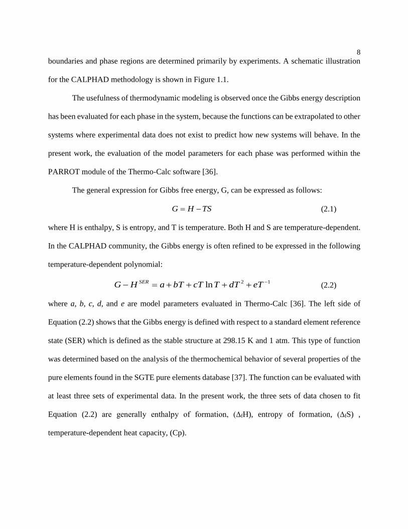
2.1 CALPHAD modeling ..................................................................................... 7
2.2 First-principles calculations based on density functional theory .................... 11 2.2.1 Density functional theory ..................................................................... 11 2.2.2 Equation of state at 0K ......................................................................... 17
2.3 Finite temperature thermodynamics ............................................................... 18 2.3.1 Debye-Grünseisen model ..................................................................... 19
2.3.2 Phonon approach .................................................................................. 23 2.3.3 Thermal electronic free energy ............................................................. 26
2.4 Diffusion theory .............................................................................................. 27
2.4.1 Diffusion overview ............................................................................... 27
2.4.2 Eyring’s reaction rate theory ................................................................ 27 2.4.3 Nudged Elastic Band (NEB) method ................................................... 29
Chapter 3 First-principles calculations and thermodynamic modeling of Sn-Sr and Mg-
Sn-Sr systems........................................................................................................ 30
3.1 Introduction ..................................................................................................... 30 3.2 Literature Review ........................................................................................... 32 3.3 Calculation and modeling details .................................................................... 36
3.3.1 First-principles calculations .................................................................. 36 3.3.2 CALPHAD modeling ........................................................................... 41
3.4 Results and Discussion ................................................................................... 45 3.5 Conclusions..................................................................................................... 49
Chapter 4 First-principles calculations and thermodynamic modeling of Ce-Sn system
with extension to Mg-Ce-Sn system ..................................................................... 74
4.1 Introduction ..................................................................................................... 74 4.2 Literature Review ........................................................................................... 75 4.3 Calculation and modeling details .................................................................... 76
4.3.1 First-principles calculations .................................................................. 76

vi
4.3.2 CALPHAD modeling ........................................................................... 79 4.4 Results and Discussion ................................................................................... 81 4.5 Conclusions..................................................................................................... 82
Chapter 5 First-principles calculations of the self-diffusion coefficients in hcp Mg 92
5.1 Introduction ..................................................................................................... 92 5.2 Diffusion theory in hcp ................................................................................... 93
5.2.1 Vacancy concentration ......................................................................... 94 5.2.2 Jump frequencies of solutes .................................................................. 94
5.3 Computational details ..................................................................................... 95 5.3.1 Supercell size and k-point density ........................................................ 95
5.3.2 Transition state search .......................................................................... 96 5.3.3 The quasi-harmonic approach .............................................................. 97
5.4 Results and Discussion ................................................................................... 99 5.4.1 Thermodynamic properties of pure hcp Mg ......................................... 99
5.4.2 Vacancy formation energy in pure Mg ................................................. 100 5.4.2 Effects of X-C functionals .................................................................... 101
5.4.3 Comparison between Debye and phonon model .................................. 103 5.5 Conclusion ...................................................................................................... 103
Chapter 6 First-principles predictions of dilute tracer diffusion coefficients of non-rare
earth elements in hcp Mg ...................................................................................... 109
6.1 Introduction ..................................................................................................... 109 6.2 Diffusion theory .............................................................................................. 111
6.2.1 Vacancy concentration adjacent to a solute atom ................................. 113
6.2.2 Jump frequencies of solutes .................................................................. 114 6.2.3 Correlation factors and the 8-frequency model .................................... 114
6.3 Computational details ..................................................................................... 117 6.3.1 Supercell size and k-point density ........................................................ 117
6.3.2 Transition state search .......................................................................... 118 6.3.3 The quasi-harmonic approach .............................................................. 118
6.4 Results and Discussion ................................................................................... 121 6.4.1 Solute-vacancy binding energy ............................................................ 121 6.4.2 Effects of X-C functionals .................................................................... 123
6.4.3 Effects of correlation ............................................................................ 124
6.4.4 Bonding and trends in calculated diffusion data .................................. 126
6.5 Conclusions..................................................................................................... 128
Chapter 7 First-principles predictions of dilute tracer diffusion coefficients of rare earth
elements in hcp Mg ............................................................................................... 153
7.1 Introduction ..................................................................................................... 153 7.2 Diffusion theory .............................................................................................. 154 7.3 Computational details ..................................................................................... 156

vii
7.4 Results and discussion .................................................................................... 158 7.4.1 Solute-vacancy binding energy ............................................................ 158 7.4.2 Correlation effects and correlation energy ........................................... 158
7.4.3 Diffusion data ....................................................................................... 160 7.5 Conclusions..................................................................................................... 161
Chapter 8 Conclusions and future work ....................................................................... 178
8.1 Summary and final conclusions ...................................................................... 178 8.2 Directions for future work .............................................................................. 180
Appendix A Thermo-Calc Mg-Sn-Sr database ........................................................... 181
Appendix B Thermo-Calc Mg-Ce-Sn database .......................................................... 189
Bibliography ................................................................................................................ 199

viii
LIST OF FIGURES
Figure 1.1. Schematics showing the materials modeling information flow based on ICME.
The properties in red color are the ones investigated in the present work. .......... 2
Figure 2.1 Schematic diagram illustrating the CALPHAD methodology ................... 10
Figure 2.2. A flow chart demonstrating the procedures of self-consistent electronic
structure calculations based on DFT. .................................................................... 15
Figure 2.3 Schematic illustration of a close-packed plane of atoms where A: the diffusing
atom is adjacent to a vacancy in a normal lattice position and B: the diffusing atom is
in the high-energy state between its initial position and the vacancy site, known as the
“transition state” or “saddle point”. ...................................................................... 28
Figure 3.1. Mg-Sn binary phase diagram calculated from the data sets given in Ref. [78].56
Figure 3.2. Mg-Sr binary phase diagram calculated from the data sets given in Ref. [79].57
Figure 3.3. Phonon dispersion curves with phonon density of states of the MgSnSr
compound calculated from the supercell method. ................................................ 58
Figure 3.4. Enthalpies of formation fH298 of the intermetallic compounds in the Sn-Sr
system at 298 K from the present finite temperature first-principles calculations
(circles) and CALPHAD modeling (line). ............................................................ 59
Figure 3.5. Absolute entropies S298 for the stable solid phases in the Sn-Sr system at 298K
from the present finite temperature first-principles calculations (circles) and
CALPHAD modeling (line). ................................................................................. 60
Figure 3.6. (a) Temperature dependence of heat capacities for all the stoichiometric
compounds in the Mg-Sn-Sr system from CALPHAD modeling and first-principles
Debye model by solid and dashed lines, respectively. (b) Heat capacity of SnSr from
the present CALPHAD modeling in comparison with that obtained from the
Neumann-Kopp approximation. The kink corresponds to the melting point of β-Sn.62
Figure 3.7, Enthalpy of formation of the solid solution phases from the present CALPHAD
modeling (lines) together with the dilute enthalpies of formation from first-principles
(circles). ................................................................................................................ 63
Figure 3.8. (a) Calculated enthalpy of mixing in the liquid at 1600 K. (b) Calculated entropy
of mixing in the liquid at 2000, 1600, 1200, and 800 K from the present CALPHAD
modeling. The liquid phase at 1200 and 800 K is metastable. ............................. 65
Figure 3.9. Mole fractions of species in liquid as a function of total Sr concentration at
1600 K, calculated from the present CALPHAD modeling. ................................ 66
ix
Figure 3.10. Calculated partial enthalpy of dissolving solid Sr at infinite dilution in liquid
Sn with the experimental data............................................................................... 67
Figure 3.11. Calculated phase diagram of the Sn-Sr system in the present work compared
with experimental data from Ref. [106]. .............................................................. 68
Figure 3.12. Calculated isothermal sections of the Mg-Sn-Sr phase diagram at 298.15 K:
(a) isothermal section of the whole composition range and (b) an enlarged isothermal
section at Mg-rich corner. ..................................................................................... 70
Figure 3.13. Calculated liquidus projection of the Mg-Sn-Sr system with isotherms (˚C).71
Figure 3.14. Calculated isopleth of Mg2Sn-Mg2Sr. ..................................................... 72
Figure 3.15. Calculated mole fraction of solid phases versus temperature curves using
Scheil simulation for alloys with two compositions: (a) Mg-10Sn-1Sr (b) Mg-10Sn-
3Sr (wt%). ............................................................................................................. 73
Figure 4.1. Mg-Sn binary phase diagram calculated from the data sets given in Ref. [78] .83
Figure 4.2. Mg-Ce binary phase diagram calculated from the data sets given in Ref. [108].
.............................................................................................................................. 84
Figure 4.3 Calculated Ce-Sn binary phase diagram from the present thermodynamic
modeling. .............................................................................................................. 85
Figure 4.4 enthalpies of formation of the Ce-Sn binary system at 298K. ................... 86
Figure 4.5 Enthalpy of mixing in the liquid phase of Ce-Sn binary system at 1870K. 87
Figure 4.6 Calculated heat capacities and entropies from first-principles based Debye
model for compound CeSn3 and Ce3Sn5. .............................................................. 88
Figure 4.7 Isothermal section and the Mg-rich corner of the Mg-Ce-Sn system at 793K 89
Figure 4.8 Liquidus projection of Mg-Ce-Sn system .................................................. 90
Figure 4.9 Scheil simulation of Mg-Ce-Sn alloys. ...................................................... 91
Figure 5.1. Illustration of vacancy-mediated diffusion jump components in an hcp lattice
showing different jump distances ( B , Ab , and Az ). The atom in the middle can
exchange position with vacancies (red arrows) either within the same basal plane at a
distance of B a , or between adjacent basal planes at distances of / 3Ab a along
the basal plane and / 2Az c along the c-axis. The jump components along basal plane
with jump distances B and Ab contribute to the diffusion coefficient D ( c-

x
axis), while the jump component along distance Az contributes to the diffusion
coefficient D (‖ c-axis). ....................................................................................... 105
Figure 5.2 Predicted heat capacity Cp and entropy S of pure hcp Mg using Debye and
phonon model in comparison with SGTE experimental data. .............................. 106
Figure 5.3 Vacancy formation (a) enthalpy, (b) free energy, (c) entropy, and (d) vacancy
concentration as a function of temperature in pure hcp Mg calculated by the X-C
functional of PBEsol using quasi-harmonic Debye model. Experimental vacancy
concentration data of Mg are taken from Janot et al. [131] and Hautojärvi et al. [134].
.............................................................................................................................. 107
Figure 5.4. Predicted self-diffusion coefficients in Mg from different X-C functionals of
LDA, GGA, and PBEsol compared with experimental data in the literature. Calculated
results with PBEsol Debye and PBEsol phonon are from the present work (black lines),
results with GGA (blue lines) and LDA (pink lines) are from Ganeshan et al. [33].
Experimental data are taken from Shewmon [114,115], Combronde and Brebec [129],
and Kulkarni et al. [117]. ...................................................................................... 108
Figure 6.1. 49 alloying elements in dilute hcp Mg studied in the present work together with
available experiments of diffusion data (see Table 6.4 for details) denoted in the
periodic table. The elemental names indicate the recommended standard potentials
supplied by VASP used in the present work for each element. The extensions sv, pv,
and d mean the semi-core s, p, and d states are treated as valence states as well,
respectively. Note that the diffusion coefficients of Ba and K were not calculated
because their direct migration barriers are vanishingly small. ............................. 136
Figure 6.2 Energy convergence as a function of KPOINTS for (a) a 64 atom supercell (b)
a 96 atom supercell. .............................................................................................. 137
Figure 6.3. Illustration of the eight possible vacancy exchanges in an hcp lattice for vacancy
and solute starting (a) within the basal plane and (b) between adjacent basal planes.
X , X are the jump frequencies for the solutes (X) and a , b , c , a , b ,
c are the jump frequencies for the solvents (Mg). ........................................... 138
Figure 6.4. Calculated solute-vacancy binding energies basal
bindE of various solutes within the
basal plane of hcp Mg as a function of atomic number. ....................................... 139
Figure 6.5. (a) Predicted diffusion coefficients of Ca and Zn in Mg with and without
correlation effects considered. Note that Zn diffusion coefficients with and without
correlation effects almost overlap with each other. (b) Calculated correlation factors
Bxf , Abf , and Azf of Zn and Ca diffusion in Mg. Note that for the Ca correlation
factors, Abf and Azf have very similar values. ................................................... 140
xi
Figure 6.6. Calculated basal migration barrier XE for each solute X in the dilute Mg63X
(Mg95X for Ba, Bi, Ca, K, Pb, Sr, and Y) systems as a function of solute induced
volume difference XV . ........................................................................................ 141
Figure 6.7. Predicted dilute solute tracer diffusion coefficients of (a) Al, (b) Zn, and (c) Sn
in Mg along with available experimental data. Results with LDA are from Ganeshan
et al. [24]. Al diffusion data are taken from Brennan et al. [159,160], Kammerer et al.
[161], and Das et al. [162]; Zn diffusion data are taken from Lal [158], Čermák and
Stloukal [168], Kammerer et al. [161], and Das et al. [169]; Sn diffusion data are taken
from Combronde and Brebec [155]. ..................................................................... 143
Figure 6.8. Predicted basal dilute solute tracer diffusion coefficients D of 47 solutes in
hcp Mg. The basal self-diffusion coefficient of Mg is plotted in a dashed line. .. 144
Figure 6.9. Calculated activation energies Q of basal diffusion coefficients of various
solutes in Mg as a function of atomic number, see Table 3.3 for values. ............. 145
Figure 6.10. Basal diffusion coefficients D at 800K for each solute in the dilute Mg63X
(Mg95X for Bi, Ca, Pb, Sr, and Y) systems as a function of bulk modulus. ......... 146
Figure 6.11. The ratio of predicted basal dilute solute diffusion coefficient over the non-
basal one, D/ D , for 47 solutes in hcp Mg. The ratio of self-diffusion coefficients of
Mg is plotted in a dashed line. .............................................................................. 147
Figure 6.12 Predicted Ag diffusion coefficients in Mg with available experimental data
taken from Lal [158] and Combronde and Brebec [155]. .................................... 148
Figure 6.13 Predicted Be diffusion coefficients in Mg with available experimental data
taken from Yerko et al [163]. ............................................................................... 148
Figure 6.14 Predicted Cd diffusion coefficients in Mg with available experimental data
taken from Combronde and Brebec [155]. ........................................................... 149
Figure 6.15 Predicted In diffusion coefficients in Mg with available experimental data
taken from Lal [158] and Combronde and Brebec [155]. .................................... 149
Figure 6.16 Predicted Fe diffusion coefficients in Mg with available experimental data
taken from Pavlinov et al. [164]. .......................................................................... 150
Figure 6.17 Predicted Ga diffusion coefficients in Mg with available experimental data
taken from Stloukal and Čermák [165]. ............................................................... 150
Figure 6.18 Predicted Mn diffusion coefficients in Mg with available experimental data
taken from Fujikawa [166]. .................................................................................. 151

xii
Figure 6.19. Predicted Ni diffusion coefficients in Mg with available experimental data
taken from Pavlinov et al. [164]. .......................................................................... 151
Figure 6.20 Predicted Sb diffusion coefficients in Mg with available experimental data
taken from Combronde and Brebec [155]. ........................................................... 152
Figure 6.21 Predicted Y diffusion coefficients in Mg with available experimental data taken
from Das et al. [167]. ............................................................................................ 152
Figure 7.1 17 alloying elements in dilute hcp Mg studied in the present work together with
available experiments of diffusion data (see Table 7.3 for details) denoted in the
periodic table. The elemental names indicate the recommended standard potentials
supplied by VASP used in the present work for each element. The extension sv means
the semi-core s state is treated as valence state as well. The extension “_3” means the
f-electrons are kept frozen in the core by adopting a valence of 3 for the ions. ... 166
Figure 7.2 Calculated basal diffusion coefficients of rare earth elements form the present
first-principles calculations. .................................................................................. 167
Figure 7.3 Calculated basal activation energy of rare earth elements in Mg ............... 168
Figure 7.4 Calculated diffusion coefficients of La in Mg compared with experiments [158].
.............................................................................................................................. 169
Figure 7.5 Calculated Ce diffusion coefficients in Mg compared with experiments [158].170
Figure 7.6 Calculated Gd diffusion coefficients in Mg compared with recent experiments
[167]. ..................................................................................................................... 171
Figure 7.7 Calculated basal solute-vacancy binding energy as a function of atomic number.
.............................................................................................................................. 172
Figure 7.8 First-principles predicted basal solute migration barrier as a function of solute
induced volume difference. .................................................................................. 173
Figure 7.9 Calculated diffusion cofficients at 800K as a function of predicted bulk modulus
in Mg95X supercells. ............................................................................................ 174
Figure 7.10 Calculated correlation factors of Lu and La diffusion in Mg. Note that in both
cases, Abf and Azf almost overlap with each other. ........................................... 175
Figure 7.11 Calculated La and Lu diffusion coefficients in Mg with/without correlation
effects considered. ................................................................................................ 176
Figure 7.12 Contributions (vacancy formation energy, vacancy migration energy, and
correlation energy) to the normal activation energies for Mg self-diffusion, Ca, and
RE solute diffusion. .............................................................................................. 177
xiii
LIST OF TABLES
Table 3.1 Solid phases of the Mg-Sn-Sr system and their crystallographic data [76] . 50
Table 3.2 First-principles results of lattice parameters and enthalpies of formation of the
intermetallic compounds in the Mg-Sn-Sr system and their Standard Element
Reference (SER) states, hcp-Mg, fcc-Sr and bct-Sn, along with the available
experimental and theoretical data from the literatures. FP=First-principles. ....... 51
Table 3.3 Calculated properties of intermetallic phases and pure elements in Mg-Sn-Sr
system at 0K from first-principles phonon and Debye model in comparison with
available experimental data, including volume (V), bulk modulus (B), first derivative
of bulk modulus with respect to pressure (B’), and Debye temperature (Θ𝐷) together
with details of first-principles calculations of each phases, including k-point mesh for
electronic structure calculations, supercell size, and k-point mesh for phonon
calculations. .......................................................................................................... 52
Table 3.4 Thermodynamic parameters of the Mg-Sn-Sr ternary system (in S.I. units) 53
Table 3.5 Summary of invariant reactions in the Sn-Sr system. .................................. 55
Table 5.1 Comparison of experimental and first-principles calculated vacancy formation
energies 0
fE and equilibrium lattice parameters a0 and c0 in hcp Mg. First-principles
results are calculated using different X-C functionals of LDA, GGA, and PBEsol at 0
K and with various supercell sizes. Note that the experimentally measured vacancy
formation energies are usually assumed to be constant with respect to temperature.104
Table 6.1 Supercell size convergence of basal and normal solute-vacancy binding energies
for Zn and Y. basal
bindE and normal
bindE are the solute-vacancy binding energies of solute and
vacancy on the same basal plane and between adjacent basal planes of hcp Mg,
respectively. .......................................................................................................... 130
Table 6.2 First-principles predicted properties of solutes in hcp Mg by the X-C functional
of PBEsol, including the volume difference, bulk modulus, solute-vacancy binding
energies and migration barriers. Here, XV indicates the volume difference induced
by placing a single solute into pure Mg, see Eq.(6.19). B is the bulk modulus of Mg63X
(Mg95X for Ba, Bi, Ca, K, Pb, Sr, and Y). basal
bindE and normal
bindE are the solute-vacancy
binding energies of solute and vacancy on the same basal plane and between adjacent
basal planes of hcp Mg, respectively. XE and XE are the solute migration barriers for
solute-vacancy exchange within the basal plane and between adjacent basal planes,
respectively. mixE is the dilute mixing energy given in units of eV per atom of solute.
S is the maximum solid solubility of each element in Mg from experiments [157]. 131
xiv
Table 6.3 Energy barriers (eV) of vacancy migration for various solutes in hcp Mg. The
subscripts refer to the migration pathways indicated in Figure 6.3. ..................... 133
Table 6.4 Predicted dilute solute (impurity) diffusion coefficients by the X-C functional of
PBEsol compared with available experimental values. 0D
and 0D are the diffusion
pre-factors (m2/s) for the diffusion components perpendicular and parallel to the c axis,
respectively. Q and Q are the diffusion activation energies (kJ/mol) for the
diffusion components perpendicular and parallel to the c axis, respectively. T-range is
the temperature range in which the experimental measurements were performed. If
only one set of average D0 and Q data is listed for a solute, it indicates that the data
was measured from polycrystalline Mg sample without anisotropy. ................... 134
Table 7.1 First-principles predicted properties of solutes in hcp Mg by the X-C functional
of PBEsol, including the volume difference, bulk modulus, and solute-vacancy
binding energies. Here, XV indicates the volume difference induced by placing a
single solute into pure Mg. B is the bulk modulus of Mg95X. basal
bindE and normal
bindE are
the solute-vacancy binding energies of solute and vacancy on the same basal plane and
between adjacent basal planes of hcp Mg, respectively. ...................................... 163
Table 7.2 Energy barriers (eV) of vacancy migration for various RE solutes in hcp Mg. The
subscripts refer to the migration pathways indicated in Figure 6.3. ..................... 164
Table 7.3 Predicted dilute RE solute (impurity) diffusion coefficients by the X-C functional
of PBEsol compared with available experimental values. 0D and 0D are the
diffusion pre-factors (m2/s) for the diffusion components perpendicular and parallel to
the c axis, respectively. Q and Q are the diffusion activation energies (kJ/mol) for
the diffusion components perpendicular and parallel to the c axis, respectively. If only
one set of average D0 and Q data is listed for a solute, it indicates that the data was
measured from polycrystalline Mg sample without anisotropy. .......................... 165
xv
ACKNOWLEDGEMENTS
Life is a wonderful journey. The people you meet during the journey can make all the
difference. There are many people I want to thank.
First of all, I want to express my sincere thanks to my PhD advisor Dr. Zi-Kui Liu. I am
deeply grateful for his guidance and generous support during my PhD career. I want to thank him
for all the doors and opportunities he opened up for me. Not only did he teach me thermodynamics
and how to do top-notch scientific research, but also the philosophy and positive attitude towards
life (his TKC theory!), from which I will benefit for the rest of my life.
The committee members of my PhD dissertation, including Dr. Jorge Sofo, Dr. Tarasankar
Debroy, and Dr. Long-Qing Chen, for their time devoted to reading my dissertation and for their
constructive criticism and thoughtful advice.
I also want to express my deepest thanks to my parents. There were lots of ups and downs
in my pursuit of a career in academic research. My parents are always there for me when I am
facing challenges. Their endless love and understanding is my unlimited source of motivation and
inspiration. I owe most of my accomplishments to them.
I would also like to thank the great lab mates in Phases Research Lab. Dr. Shun-Li Shang
is my main mentor besides Dr. Liu. He gave me lots of technical help with first-principles
calculations and helped me greatly with my paper writing skills. I enjoyed the friendship with all
the old and new members in Phases Research Lab during my PhD study. I want to thank Dr. James
Saal with the discussions and his invitation to intern at QuesTek Innovations, Dr. Sunghoon Lee
for teaching me about oxides modeling, Drs. Hui Zhang and Guang Sheng, Dr. Arkapol
Saengdeejing, Dr. Chelsey Hargather for her help with my paper writing, Dr. Huazhi Fang for

xvi
helping me with the diffusion calculations, Dr. Xuan Liu and Yong-Jie for valuable discussion and
sharing their passion on Metallurgy, Kang for stimulating discussions on statistical mechanics and
phase transformations.
My friends in State College, especially Yong-Jie, Fei, and Lei, PhD life was difficult and
challenging, but with friendship the journey was much more fun and more enjoyable. Thanks to
you guys, the time we shared together makes great memories.
Lastly I want to express my deep gratitude to Prof. Yong Du in Central South University.
If I didn’t join his research lab as an undergraduate student I wouldn’t have the chance to find my
lifelong passion, computational materials science, so early in my life. Thank you so much for
introducing such a wonderful field to me.
1
Chapter 1
Introduction
1.1 Motivation
In recent years, magnesium (Mg) alloys have received an increasing interest due to their
low density, earth abundance, high specific strength, and good castability [1]. Mg ion is the most
abundant and extractable structural metallic ion the ocean [2]. These properties make Mg alloys
attractive for automotive, aerospace, and other light-weight structural applications [3]. Mg and its
alloys have great potential for considerably reducing the weight of transportation vehicles,
improving their fuel efficiency, and making them more environmentally friendly [3]. The world
consumption of Mg alloys in the automobile industry has experienced a 15% annual increase over
the last decade [4]. It is also a bioabsorbable metallic element and can be metabolized by human
body. There are significant efforts in making bioabsorbable materials using controlled corrosion
in Mg alloys for cardiovascular stent applications [5].
Despite these tantalizing opportunities, there are mainly three challenges to the wider use
of Mg alloys [6]:
1. limited precipitation strengthening
2. poor low temperature formability
3. corrosion and dissimilar joining issues

2
The poor low temperature formability is due to the limited slip systems in the hexagonal
closed packed (hcp) Mg. Since Mg has very low electronegativity, it is easy to react with other
metals, especially when it is joined with other materials such as Al [6].
To overcome these issues and accelerate the development of better cast and wrought Mg
alloys, better computational materials design tools and more reliable materials data are needed. As
emphasized in the Materials Genome Initiative (MGI) [7] and the Integrated Computational
Materials Engineering (ICME) framework [8], the integration of computational and experimental
investigations is the key to efficiently develop fundamental understanding of materials behaviors
and the material data infrastructure. Figure 1.1 below shows a schematic figure of the materials
modeling process based on the concept of ICME.
Figure 1.1. Schematics showing the materials modeling information flow based on ICME. The
properties in red color are the ones investigated in the present work.
The majority of Mg alloys derives their mechanical properties from precipitation hardening
[9]. The study of precipitation process demands accurate thermodynamic and kinetic (diffusion)
3
data. Thermodynamics of Mg alloys has been extensively studied, and several comprehensive
thermodynamic databases have been established [10] based on the CALculation of PHAse
Diagram (CALPHAD) modeling technique [11,12]. The CALPHAD technique predicts the
thermodynamic properties of a multi-component system from extrapolation of the constituent
binary and ternary Gibbs energy descriptions, where experimental data is usually more plentiful.
With this method, the properties of complex alloys can be efficiently and accurately predicted in
a reduced amount of time compared to an equivalent experimental investigation. A further
contribution of the current thermodynamic database in the present work would be the Mg-Sn based
systems (e.g. Mg-Sn-Sr and Mg-Ce-Sn systems) for high-temperature applications.
However, the kinetics of Mg alloys has been studied to a far lesser extent, especially
diffusion coefficients of various solutes in Mg. Due to the issues related to corrosion, oxidation,
and contamination during sample preparation in diffusion measurements, few experimental data
are available in the literature for diffusion coefficients of solutes in Mg [13]. Although recently a
diffusion mobility database for Mg alloys was published [14], diffusion data are still lacking for
most of the solutes in Mg alloys. This greatly hinders the development of new Mg alloys.
For the investigation of kinetic processes in Mg alloys in the solid state, such as creep [15],
solute strengthening [16,17], solution treatment and aging [18], reliable diffusion data and detailed
insights into diffusion of solutes in Mg are desperately needed. For example, the knowledge of
diffusion coefficients can help to determine the desirable aging time to achieve peak hardness in
precipitation-hardened Mg alloys [9]. Wrought Mg alloys have seen very little implementation in
the automotive industry because of their poor formability at room temperature [15] as mentioned
before. To improve the formability of wrought Mg alloys, proper alloying additions can be selected
by evaluating their solute drag propensity at the grain boundaries [19] to mitigate the basal plane

4
texture formation due to the inhomogeneous deformation of hcp Mg. This propensity greatly
depends on their diffusion coefficients based on Cahn’s solute drag theory [11]. Diffusion of
solutes around the dislocation core structure in Mg also plays an important role in understanding
the origin of many plastic phenomena such as dynamic strain aging [17] and plastic instabilities
[20]. Therefore, the information of solute diffusion coefficients in Mg is critical for the
development of new casting and wrought Mg alloys.
Fortunately, it is now possible to calculate many aspects of diffusion [21,22]. First-
principles calculations based on density functional theory (DFT) have been extensively used to
calculate diffusion coefficients, especially when experimental data are lacking [23,24]. These
calculations are usually coupled with transition state theory (TST) under the harmonic or the quasi-
harmonic approximations [22]. TST has become a practical tool in the context of DFT calculations
when efficient algorithms for finding the minimum-energy path have been developed, such as the
nudged elastic band (NEB) and the climb image nudged elastic band (CI-NEB) method [25]. At
present, first-principles calculations of diffusion coefficients are largely limited to cubic systems,
such as those in Al [23,26], Fe [27,28], and Ni [29–31] alloys. This is due to the additional
complexity of anisotropy associated with the calculations of diffusion coefficients in hcp systems.
Recently, Ganeshan et al. [24] in our group calculated the diffusion coefficients of Al, Zn, Sn, and
Ca in dilute hcp Mg using an 8-frequency model. However, their calculated results compared with
experimental data still need to be further improved (see details in Chapter 5 and Chapter 6), and
especially more alloying elements need to be considered for Mg alloys.

5
1.2 Objectives
The overarching goal of the present study is to investigate the effects of alloying elements
on the thermodynamic and diffusion properties of Mg alloys using CALPHAD approach and first-
principles calculations based on DFT.
For the thermodynamic properties, we plan to build the thermodynamic databases of the
Mg-Sn-Sr and Mg-Ce-Sn alloy systems using the well-established CALPHAD approach with key
thermodynamic properties calculated from finite temperature first-principles calculations. For the
diffusion properties, we use first-principles calculations coupled with the TST and the 8-frequency
model to calculate the dilute solute tracer diffusion coefficients in hcp Mg. Sixty-one substitutional
alloying elements have been considered herein, namely Ag, Al, As, Au, Be, Bi, Ca, Cd, Co, Cr,
Cu, Fe, Ga, Ge, Hf, Hg, In, Ir, Li, Mn, Mo, Na, Nb, Ni, Os, Pb, Pd, Pt, Re, Rh, Ru, Sb, Sc, Se, Si,
Sn, Sr, Ta, Tc, Te, Ti, Tl, V, W, Y, Zn, Zr, and rare earth elements La, Ce, Pr, Nd, Pm, Sm, Eu,
Gd, Tb, Dy, Ho, Er, Tm, Yb, Lu (see also Figure 6.1 and Figure 7.1). The self-diffusion coefficient
of Mg has been calculated as well. The effects of different exchange-correlation (X-C) functionals
on diffusion properties are examined. It is shown that the recently developed PBEsol X-C
functional [32] yields better agreement with experimental data compared with the commonly used
X-C functionals such as the local density approximation (LDA) and the generalized gradient
approximation (GGA) for the self-diffusion [33] and solute diffusion coefficients (Al, Sn, Zn) in
Mg [24] calculated in previous works. The vibrational properties are derived from the quasi-
harmonic Debye model [34,35]. Therefore, we are able to calculate not only the migration barriers
but also the temperature-dependent jump frequencies and the diffusion pre-factors, which are
related to vibrational entropic contributions. Finally the dilute solute tracer diffusion coefficients
in hcp Mg are calculated. The diffusion pre-factors and the activation energies are obtained by
6
fitting the calculated diffusion coefficients to the Arrhenius-type diffusion equation (see details in
Chapter 6).
1.3 Organization
The contents of this thesis are organized as follows. Chapter 2 is the methodology section.
It includes a detailed methodology for the thermodynamic modeling using the CALPHAD
approach, the background and details for all type of first-principles calculations used in the
CALPHAD modeling and for first-principles calculations of diffusion coefficients. It also
introduces basic diffusion theory in hexagonal close-packed systems. Specifics for each type of
calculation as well as the diffusion equations for calculating pertinent properties are given in the
relevant chapters. Chapter 3 and Chapter 4 present the first-principles calculations supplemented
thermodynamic modeling of the Mg-Sn-Sr and Mg-Ce-Sn systems, respectively, showing the
value of adding first-principles calculated properties to obtaining a more accurate thermodynamic
description of the system. Chapter 5 validates the diffusion coefficient calculation procedure by
presenting the first-principles predicted vacancy concentration and diffusion coefficient for self-
diffusion in hcp Mg. Following the most successful methodology demonstrated in Chapter 5,
Chapter 6 presented the results of the 47 Mg-X non-rare earth impurity diffusion coefficient
calculations from first-principles. Chapter 7 the results of the 14 Mg-X rare earth diffusion
coefficient calculations from first-principles. Effects of correlation on the calculated diffusion
coefficients are discussed. Finally, Chapter 8 concludes this thesis by presenting a summary of all
of the work done and recommendations for possible areas for the future work on the first-principles
calculations of self-, impurity, and non-dilute impurity diffusion coefficients are provided.
7
Chapter 2
Computational methodology
In this chapter, the computational methodology is given in order to reproduce the results
obtained in this dissertation. First, the theory of thermodynamic modeling is presented, including
an overview of the CALPHAD technique and the details of the parameterization of the Gibbs
energy functions used for each phase. Then an overview of DFT and the associated finite
temperature thermodynamic models used in both the CALPHAD modeling and the diffusion
coefficient calculations is given. The chapter concludes with a review of diffusion theory and the
relevant equations and assumptions, while a more detailed procedure will be given in each
respective chapter of self-diffusion and dilute solute diffusion.
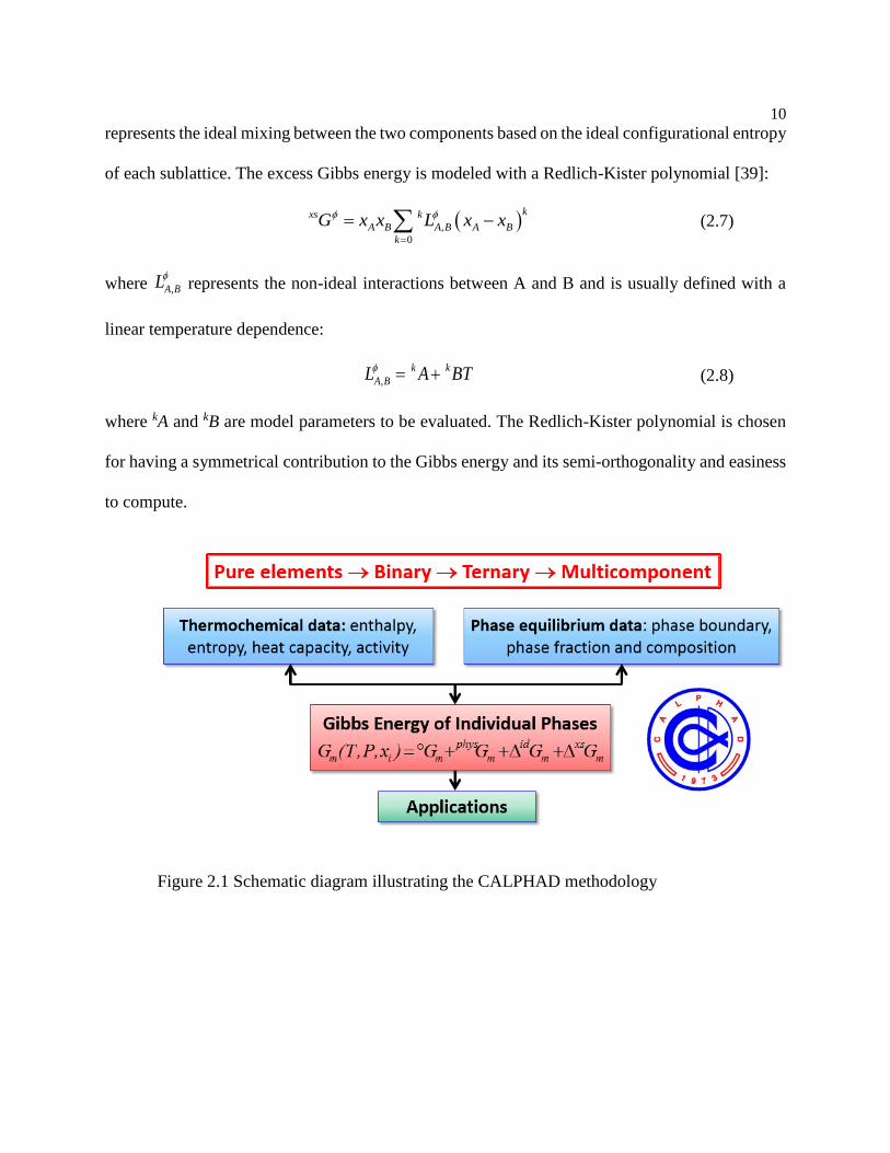
2.1 CALPHAD modeling
Thermodynamic modeling based on the CALPHAD methodology parameterizes the Gibbs
free energy functions of the individual phases in the systems of interest as temperature (T), pressure
(P), and composition (x) dependent expressions. Thermochemical data of individual phases and
phase equilibrium data between phases are fit to the expressions to determine the model
parameters. Thermochemical data used to evaluate a single phase could be experimentally
measured heat capacity, activity, or other property, or the theoretical data from first-principles
calculations if the experimental data is missing or unreliable. Phase equilibrium data such as phase
8
boundaries and phase regions are determined primarily by experiments. A schematic illustration
for the CALPHAD methodology is shown in Figure 1.1.
The usefulness of thermodynamic modeling is observed once the Gibbs energy description
has been evaluated for each phase in the system, because the functions can be extrapolated to other
systems where experimental data does not exist to predict how new systems will behave. In the
present work, the evaluation of the model parameters for each phase was performed within the
PARROT module of the Thermo-Calc software [36].
The general expression for Gibbs free energy, G, can be expressed as follows:
G H TS (2.1)
where H is enthalpy, S is entropy, and T is temperature. Both H and S are temperature-dependent.
In the CALPHAD community, the Gibbs energy is often refined to be expressed in the following
temperature-dependent polynomial:
2 1lnSERG H a bT cT T dT eT (2.2)
where a, b, c, d, and e are model parameters evaluated in Thermo-Calc [36]. The left side of
Equation (2.2) shows that the Gibbs energy is defined with respect to a standard element reference
state (SER) which is defined as the stable structure at 298.15 K and 1 atm. This type of function
was determined based on the analysis of the thermochemical behavior of several properties of the
pure elements found in the SGTE pure elements database [37]. The function can be evaluated with
at least three sets of experimental data. In the present work, the three sets of data chosen to fit
Equation (2.2) are generally enthalpy of formation, (∆fH), entropy of formation, (∆fS) ,
temperature-dependent heat capacity, (Cp).
9
To fit the experimental or first-principles data according to Equation 2.2, the equation must
be transformed to represent the various thermodynamic quantities. First, entropy is the negative
first derivative of Gibbs energy with respect to temperature and is given as:
2ln 2dG
S b c c T dT eTdT
(2.3)
Second, enthalpy can be derived by plugging Equation (2.2) and Equation (2.3) into
Equation (2.1) and then solving for H, which yields:
2 12H G TS a cT dT eT (2.4)
Third and finally, heat capacity can be derived as the first derivative of enthalpy, or the
second derivative of Gibbs energy with respect to temperature times the negative of temperature:
2
2
22 2p
dH d GC T c dT eT
dT dT
(2.5)
In solution phases, the compound energy formalism [38] is employed to represent the
change in composition in a single phase via sublattice models. In the present work, the sublattices
are necessitated by the fact that in a solution phase in a binary phase diagram such as fcc, hcp, bcc,
or liquid, can have atom A or atom B sitting on any given site, based on the composition and
crystal structure of the phase. The molar Gibbs energy of a solution phase of atoms A and B is
given by:
ln ln xs
m A A B B A A B BG x G x G RT x x x x G (2.6)
where xA and xB are the mole fractions of A and B, respectively, AG and BG are the Gibbs
energies of pure A and pure B in the structure ϕ, respectively, and xsG
is the excess Gibbs energy.
The first two terms represent the mechanical mixing of the component A and B and the third term
10
represents the ideal mixing between the two components based on the ideal configurational entropy
of each sublattice. The excess Gibbs energy is modeled with a Redlich-Kister polynomial [39]:
,
0
kxs k
A B A B A B
k
G x x L x x
(2.7)
where ,A BL represents the non-ideal interactions between A and B and is usually defined with a
linear temperature dependence:
,
k k
A BL A BT (2.8)
where kA and kB are model parameters to be evaluated. The Redlich-Kister polynomial is chosen
for having a symmetrical contribution to the Gibbs energy and its semi-orthogonality and easiness
to compute.
Figure 2.1 Schematic diagram illustrating the CALPHAD methodology
11
2.2 First-principles calculations based on density functional theory
Density functional theory total energy calculations are often known as “ab-initio”
calculations, meaning “from first principles” because the inputs are the atomic coordinates and
atomic numbers, and they do not rely on any experimental or empirical data. The total energy of
the crystalline structure is then determined by using quantum mechanical electronic theory based
on the electronic charge density. In this dissertation, the thermodynamic properties and ground
state energies calculated in this work through the use of first-principles calculations based on
density functional theory are used in several ways. In the CALPHAD modeling, the values
obtained such as entropy and enthalpy of formation as a function of temperature help to constrain
the Gibbs energy functions of various phases to realistic values, which provide a more accurate
extrapolation to higher order systems. In a different way, DFT is used to obtain the thermodynamic
properties as a function of temperature for all of the configurations necessary to calculate the
governing factors entering into vacancy mediated self- and impurity diffusion. Additionally, this
approach can be extended to solve for relative energies for phases that are not thermodynamically
stable.
2.2.1 Density functional theory
In principle, a solid can be thought of as a collection of interacting positively charged nuclei
and negatively charged electrons. Theoretically, an exact treatment of solids can be obtained by
solving the following many-body Schrödinger’s equation involving both the nuclei and the
electrons. The dynamics of a time independent non-relativistic system are governed by the
Schrödinger equation:

12
H E (2.9)
where is the many-electron wave function, E the system energy and H the Hamiltonian of the
system given by (in atomic units):
2 22 2
1
1 1
2 2
N
i
i R i ji i j
eH Ze
m r R r r
(2.10)
where ir is the position of electron i, while the nuclei are clamped at position R. The first term is
the many-body kinetic energy operator which yields the electronic kinetic energies; the second
term represents the interaction of the electrons with the bare nuclei. Electron-electron interactions
are described by the final term. We have neglected the nuclei-nuclei interaction energy in the
above, which would have to be added in order to yield the total energy of the system. However,
the Born-Oppenheimer approximation allows us to decouple the nuclear and electronic degrees of
motion; the nuclei are of order ~ 103 – 105 times massive than the electrons, and therefore may be
considered to be stationary on the electronic timescale. As a result of this, it is possible to neglect
the nuclear kinetic energy contribution to the system energy. Although this equation is exact within
the non-relativistic regime, it is not possible, except for trivially simple case, to solve it. There are
two reasons for this: one mole of a solid contains N ~ 1028 electrons; since the many-electron
wave function contains 3N degrees of freedom, this is simply intractable; further, the electron-
electron Coulomb interaction results in the electronic motions being correlated. Thus we must
search for approximations that render the Schrödinger equation tractable to numerical solution,
while retaining as much of the key physics as is possible.
Density functional theory treats the electron density as the central variable rather than the
many-body wave function. This conceptual difference leads to a remarkable reduction in difficulty:

13
the density is a function of three variables, i.e., the three Cartesian directions, rather than 3N
variables as the full many-body wave function is. Here we consider the Hohenberg-Kohn-Sham
formulation of DFT [40,41]; this technique has enjoyed success in fields ranging from quantum
chemistry and condensed matter physics to geophysics. DFT is based on the following theorems,
also called Hohenberg-Kohn (HK) theorems [40]:
Theorem I: The external potential is a unique functional of the electron density only. Thus
the Hamiltonian, and hence all ground state properties, are determined solely by the electron
density. Theorem II: The ground state energy may be obtained variationally: the density that
minimizes the total energy is the exact ground state density.
The many-body Hamiltonian H fixes the ground state of the system under consideration,
i.e., it determines the ground state many-body wavefunction Ψ, and thus the above theorem ensures
that this is also a unique function of the ground state density. Consequently, the kinetic and
electron-electron interaction energies will also be functionals of electron density ρ(r). Under HK
theorem I, the total energy functional of a many-electron system is
3
ee extE r T r E r V r r d r (2.11)
where T[ρ(r)] is the kinetic energy and Eee[ρ(r)] is the interaction energy of electrons. Although
these two theorems prove the existence of a universal functional, they do not give any idea as to
the nature of the functional, or how to actually calculate the ground state density. To solve this
problem, Kohn and Sham [41] introduced an auxiliary independent-particle system composed of
Kohn-Sham orbitals r . The sum of these orbitals equals to the particle density of the real
systems:
2
1
N
i
i
r r
(2.12)
14
where N is the number of particles. Let TS be the independent-particle kinetic energy, and then the
Kohn-Sham version of Eq. (2.11) can be rewritten as:
3
KS S Hatree ext xcE r T r E r d rV r r E r (2.13)
The term Exc[ρ(r)] includes not only the exchange and correlation energy of interacting
electrons, but also the difference between T and TS. The exact form of Exc[ρ(r)] is still unknown.
Exploiting the variational principle under HK theorem II, and introducing Lagrange multiplier
method for handling the conservation of particle number constraint, Schrödinger-like single
particle equations can be obtained
KS i i iH r r (2.14)
where
2
2
2KS i effH r V r
m (2.15)
eff Hatree ext XCV r V r V r V r (2.16)
Here
HatreeHatree
EV r
r
and
XC
XC
EV r
r
(2.17)
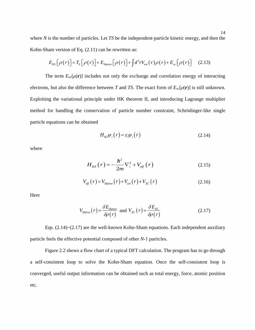
Eqs. (2.14)~(2.17) are the well-known Kohn-Sham equations. Each independent auxiliary
particle feels the effective potential composed of other N-1 particles.
Figure 2.2 shows a flow chart of a typical DFT calculation. The program has to go through
a self-consistent loop to solve the Kohn-Sham equation. Once the self-consistent loop is
converged, useful output information can be obtained such as total energy, force, atomic position
etc.

15
Figure 2.2. A flow chart demonstrating the procedures of self-consistent electronic structure
calculations based on DFT.
However, the actual form of Exc[ρ(r)] is not known; thus approximate functionals based
upon the electron density must be introduced to describe this term. One of the very early and most
widely used approximation is the Local Density Approximation (LDA), which assumes that the
exchange-correlation energy is only a functional of the local density of electrons in the form:
3LDA
xc xcE r r r d r (2.18)
with
hom
xc xcr r (2.19)
where in the last equation the assumption is that the exchange-correlation energy is purely local.
The most common parameterization in use for hom
xc is that of Perdew and Zunger [42], which is

16
based upon the quantum Monte Carlo calculations of Ceperley and Alder on homogeneous electron
gases at various densities [43]. The LDA ignores corrections to the exchange-correlation energy
due to inhomogeneity in the electron density about r. One significant limitation of LDA is its
overbinding of solids: lattice parameters are usually underestimated while cohesive energies are
usually overestimated. This issue will be further discussed in Section 5.4.2 when it relates to the
calculation of diffusion coefficients in Mg.
Another widely used approximation is the Generalized Gradient Approximation (GGA),
which attempts to incorporate the effects of inhomogeneity by including the gradient of the
electron density. The GGA exchange-correlation functional can be written as:
hom 3,GGA
xc xc xcE r r r r r r d r (2.20)
where ,xc r r is known as the enhancement factor. Unlike the LDA, there is no unique
form of the GGA, and indeed many possible variations are possible, each corresponding to a
different enhancement factor.
Efforts to obtain more accurate and efficient exchange-correlation functional never stop,
including modifications on GGAs, orbital-dependent functional, and hybrid functional [44].
Various GGA exchange correlation functionals have emerged, including PW91-GGA from
Perdew and Wang [45], PBE-GGA due to Perdew, Burke and Ernzerhof (PBE) [46], AM05-GGA
due to Armiento and Mattsson [47], and revised PBE GGA for solids (PBEsol) [32]. The basic
quantities DFT calculations can provide are the total energy, as well as their derivatives, for
example, forces and stresses. Generally speaking, PBE-GGA gives better predictions of
equilibrium properties than those by LDA. However, LDA seems predict more accurate forces and
thus phonons of oxides. The AM05 functional and the PBEsol functional are constructed using

17
different principles as implemented in VASP [48,49], but both aim at a decent description of
yellium surface energies. Therefore, they are able to better describe the surface energy of metals,
including metal vacancy which can be viewed as a small amount of internal surface in metals.
Based on our extensive tests, PBEsol is slightly more efficient computationally than AM05.
2.2.2 Equation of state at 0K
With the ability to calculate the total energy of arbitrary structures, DFT can be applied to
several models where such energies are necessary. For instance, the equation of state (EOS)
describes the dependence of a structure's energy on its volume. Details of EOSs and related
properties will be presented in this section. There have been several EOSs developed in the
literature, and each of them has specific applications. Therefore, we need to choose a suitable EOS,
based on criteria such as minimum fitting errors. The available energy-volume (E-V) EOSs can be
roughly categorized into two groups, i.e., linear and non-linear EOSs. The widely used linear EOSs
are the Birch-Murnaghan (BM) EOS [50,51] and the modified Birch-Murnaghan (mBM) EOS
[52]. Their fourth-order (five parameters) equations have the following common format:
/3 2 /3 4 /4n n n nE V a bV cV dV eV (2.21)
where a, b, c, d, and e are the fitting parameters, for third-order (four parameters) case e = 0. When
n = 2, it is the BM EOS; when n = 1, it becomes the mBM EOS proposed by Teter et al. [52].
Starting from EOS fitting to E-V, the volume-dependent pressure P, bulk modulus
B, and the first and second derivatives of bulk modulus with respect to pressure, B’ and
B’’, respectively, are obtained via,
E
P V VV
(2.22)

18
2
2
EB V V
V
(2.23)
B B P
B VV VP
(2.24)
3
2 2 2
2 22
B B P P B PB V
V V V V VP
(2.25)
As a rule of thumb, EOS fitting should be performed in a single phase region, the total
energy calculated by first-principles should be within the volume range of ±10% around the
equilibrium volume. For magnetic materials, care should be taken for the correspondingly
magnetic moment versus volume relationship: a sudden jump of magnetic moment usually
indicates a magnetic phase transition.
2.3 Finite temperature thermodynamics
In principle, DFT calculations can only predict the ground state energy of a system, E0, i.e.,
at zero temperature. To investigate thermodynamics and phase transitions at finite temperature,
free energy as a function of temperature and volume, F(V,T), is needed. The free energy is related
to the Gibbs energy by the thermodynamic relation:
, ,G P T F V T PV (2.26)
F(V,T) can be divided into several terms based on individual contribution, and each
contribution can be described by a separate model,
0, , , ,vib ele magF V T E V F V T F V T F V T (2.27)
Fvib is the free energy due to lattice vibrations, where phonons excite atoms from their
ground state positions, described in the next two subsections. Fele is the thermal electronic free
19
energy where electrons are thermally excited to excited energy states, described later in this
chapter. Fmag is the magnetic free energy where the spin states of magnetic ions can disorder.
In most cases, the largest contribution to the temperature-dependence of the free energy
arises from the lattice vibrational energy. Predicting Fvib from first-principles will be described by
two methods in this section: calculating the input parameters of the Debye-Grüneisen model or
directly calculating phonons by the supercell approach.
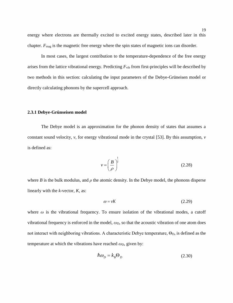
2.3.1 Debye-Grünseisen model
The Debye model is an approximation for the phonon density of states that assumes a
constant sound velocity, v, for energy vibrational mode in the crystal [53]. By this assumption, v
is defined as:
1
2Bv
(2.28)
where B is the bulk modulus, and ρ the atomic density. In the Debye model, the phonons disperse
linearly with the k-vector, K, as:
vK (2.29)
where ω is the vibrational frequency. To ensure isolation of the vibrational modes, a cutoff
vibrational frequency is enforced in the model, ωD, so that the acoustic vibration of one atom does
not interact with neighboring vibrations. A characteristic Debye temperature, ΘD, is defined as the
temperature at which the vibrations have reached ωD, given by:
D B Dk (2.30)

20
where is Planck’s constant, kB is Boltzmann’s constant. ΘD is an integral input parameter in the
Debye model, defining the region of low temperature and high temperature behavior of the model.
It is often measured experimentally as a method of characterizing the vibrational properties of a
solid. It also can be calculated from the Debye model by:
1/3
1/32 4
63
D
B
vk
(2.31)
Substituting Eq. (2.28) into the above equation and collecting all the constants into A, we
have
1/2
D
rBA
M
(2.32)
where r is the interatomic distance, M is the average atomic mass, and A is a constant, 231.1 when
B is in GPa and r is in Å. It was found, however, that the using experimental bulk modulus in
above Eq. (2.32) results in larger Debye temperatures than experiment [21]. This overestimation
is a consequence of the assumption that the v is proportional only to B in Eq. (2.32). In reality, a
crystal’s stiffness is anisotropic, characterized by transverse and longitudinal moduli, S and L,
respectively. This error can be corrected by introducing a scaling parameter, s, correcting for this
anisotropy. Equation (2.28) becomes:
1/2
Bv s
(2.33)
Therefore, we have
1/2
D
rBsA
M
(2.34)
By fitting values of S and L to linear functions of B for many nonmagnetic cubic elements,
Moruzzi et al. [53] found the relations L ~ 1.42B and S ~ 0.30B, yielding a scaling parameter, s,

21
of 0.617. However, s should not be taken as 0.617 universally as the anisotropy of the elastic
moduli will differ for different classes of materials.
The Debye model is intrinsically harmonic, where the potential energy is quadratic with
the displacement of the atoms. Ignoring anharmonic effects have large consequences on the
predicted thermodynamic properties. For instance, without anharmonicity, the Debye model
predicts a constant heat capacity above the Debye temperature. Anharmonic effects include
phonon-phonon interactions, lattice thermal expansion, and the temperature dependence of the
elastic constants.
Anharmonicity due to lattice expansion can be added to the Debye model with the addition
of the Grüneisen parameter, γ, forming the Debye-Grüneisen model. γ describes the volume-
dependence of ΘD:
ln
ln
D
V
(2.35)
Combining Eqs. (2.34) and (2.35), we have:
1 1 ln
6 2 ln
B
V
(2.36)
Plug in Eq. (2.23),
2 22 /
3 2 /
V P V
P V
(2.37)
This function for γ assumes all the modes, longitudinal and transverse, are excited and provides a
high-temperature limit for γ, γHT. At the low temperature limit, γLT, it is assumed that the transverse
modes dominate and longitudinal modes are not active, so that 1
3HT LT and we have
2 2/
12 /
LT
V P V
P V
(2.38)

22
The scaling of ΘD with volume is added to Eq. (2.34) by:
1/2
0D
VrBsA
M V
(2.39)
where V0 is the ground state volume. Since most of the phase transitions in the current work occur
at temperatures higher than ΘD, γHT will be used.
To predict the lattice vibrational contribution to the free energy from the Debye-Grüneisen
model, Fvib is defined by:
vib vib vibF E TS (2.40)
where Evib is the lattice vibrational energy, and Svib is the lattice vibrational entropy. Evib and Svib
are given by:
0 3 Dvib K BE E k TD
T
(2.41)
4
3 ln 13
D
D Tvib BS k D e
T
(2.42)
where D(x) is the Debye function:
3
3
03
1
x
t
tD x x dt
e
(2.43)
And E0K is the zero-point energy, from fluctuations at the quantum level due to the Heisenberg
uncertainty principles. This energy is defined by:
0
9
8K B DE k (2.44)
Thus, with these equations the Debye-Grüneisen model can efficiently predict the lattice
vibrational energy (and, in turn, the lattice vibrational heat capacity and entropy) where the only
23
inputs are V0, B, and B’, which are predicted by DFT from EOS fitting. Without ambiguity, the
Debye-Grüneisen model will be simply called the Debye model in this dissertation.
2.3.2 Phonon approach
Under the standard harmonic approximation, atoms are considered to only deviate slightly
from their equilibrium positions. With this approximation made, the potential energy of a system
is expanded around its equilibrium value in quadratic terms based on atomic distance. Thus the
harmonic approximation can account for all atomic interactions with other atoms in a 3 x 3 force
constant matrix.
Consider a system with N atoms and Greek letter subscripts that denote the Cartesian
components of a vector. Under the harmonic approximation, the vibrational energy of the system
can be written as [54]:
,
,
1,
2
T
vibH u i i j u j
(2.45)
The 3x3 matrices, ,i j are the force constant tensors that relate the displacement of atom j to
the force, f, exerted on atom i through:
, ,f i i j u j (2.46)
Through first-principles calculations, ,i j is determined by calculating a set of
individual atomic perturbations in a supercell. When the harmonic approximation is applied, the
force constant tensors can be written as:
2
, ,E
i ju i u j
(2.47)
24
When Eq. (2.45) is summed over all displacement u(i) over all atoms N of
atomic mass Mi, the resulting vibrational frequencies are the 3N eigenvalues of
the dynamical matrix. The vibrational free energy is based on the vibrational entropy, which is
defined as the number of thermally activated vibrational modes at a specific temperature.
Maradudin et al. [55] defines the equation for Helmholtz energy of a system under the harmonic
approximation based on the partition function of lattice vibrations as:
ln 2sinh2
j
vib B
j B
hvF T k
k T
q
q (2.48)
where Eq. (2.48) is called the vibrational free energy or kinetic energy, which gets its contributions
from the vibrational degrees of freedom of the system. The eigenvalues of dynamical matrix
,i j are the vibrational frequencies, v, and q is the wave vector. From this equation, the
vibrational enthalpy and entropy can be derived accordingly.
The information of the dynamical matrix is conveniently summarized by the phonon
density of states (DOS), which gives the number of modes of oscillation having a frequency lying
in the interval [ , ]v v dv :
3
1
1 N
n
n
g v v vN
(2.49)
The double summation in Eq. (2.48) can be written in terms of the integration of phonon DOS,
which is given by:
0
ln 2sinh2
vib B
B
hvF T k T g v dv
k T
(2.50)
Under the harmonic approximation, temperature dependence of the vibrational free energy
is described solely from the vibrational degrees of freedom, and often does not give the most
25
complete vibrational description of the system. Another limitation of the harmonic approximation
lies in the fact that in reality, a nearly infinite number of perturbations would be necessary to
accurately describe all of the phonon interactions and calculate the force constant. Thus, an
assumption is made that the most important interactions occur in the first several nearest neighbor
shells of the atoms in question, and the further away interactions are truncated from the calculation.
This is a reasonable assumption to make, and this method has shown to be quite accurate given its
limitations.
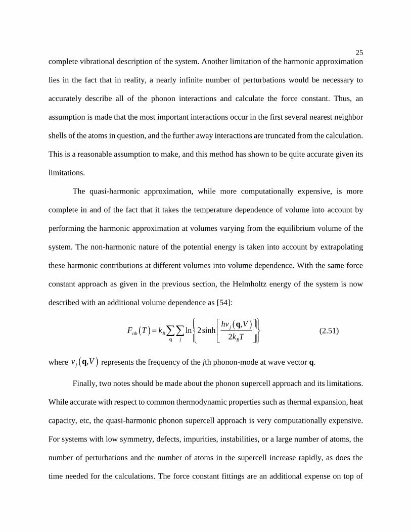
The quasi-harmonic approximation, while more computationally expensive, is more
complete in and of the fact that it takes the temperature dependence of volume into account by
performing the harmonic approximation at volumes varying from the equilibrium volume of the
system. The non-harmonic nature of the potential energy is taken into account by extrapolating
these harmonic contributions at different volumes into volume dependence. With the same force
constant approach as given in the previous section, the Helmholtz energy of the system is now
described with an additional volume dependence as [54]:
,
ln 2sinh2
j
vib B
j B
hv VF T k
k T
q
q (2.51)
where ,jv Vq represents the frequency of the jth phonon-mode at wave vector q.
Finally, two notes should be made about the phonon supercell approach and its limitations.
While accurate with respect to common thermodynamic properties such as thermal expansion, heat
capacity, etc, the quasi-harmonic phonon supercell approach is very computationally expensive.
For systems with low symmetry, defects, impurities, instabilities, or a large number of atoms, the
number of perturbations and the number of atoms in the supercell increase rapidly, as does the
time needed for the calculations. The force constant fittings are an additional expense on top of

26
the actual perturbation calculations. Additionally, dynamically unstable systems will yield
imaginary phonon frequencies, adding additional complexities when evaluating the
thermodynamic properties by integrating the phonon DOS. When one or both of these problems
are encountered, the Debye-Grüneisen model can be implemented for the sake of simplicity and
efficiency in the calculations.
2.3.3 Thermal electronic free energy
The thermal electronic contribution to the free energy, Fele, in Eq. (2.27), arises when
electrons are thermally excited to higher energy states. This contribution can be ignored for semi-
conductors and insulators as the band gap energy will typically be larger than the thermal energy,
kBT. For metals such as magnesium, this contribution must be considered.
The thermal electronic free energy can be written as:
ele ele eleF E TS (2.52)
where Eele and Sele are the energy and entropy of thermal electronic excitations, respectively. Sele
can be calculated by integrating over the energies of the excited electrons:
, , ln , 1 , ln 1 ,ele BS V T k n V f T f T f T d (2.53)
where ,n V is the electronic density at energy and f is the Fermi-Dirac distribution, given by,
1
,
exp 1B
f T
k T
(2.54)
where is the chemical potential of an electron. The thermal electronic energy is determined by,
, , , ,eleE V T n V f T d n V d
(2.55)
27
The electron density of state (EDOS) and Fermi energy are calculated from DFT.
2.4 Diffusion theory
2.4.1 Diffusion overview
The present work focuses on vacancy-mediated diffusion in a crystalline solid and
calculates the least energy diffusion path of an atom between the initial and final states of an
elementary atomic jump. Essentially, two processes are occurring. Firstly, a vacancy needs to
form. Secondly, a thermally activated jump is occurring where the jumping atom and the first
nearest neighbor vacancy exchange lattice sites, known as vacancy migration. In the case of dilute
solute diffusion, one solute atom is inserted into the supercell. In hcp crystals, this creates 2
possible types of jumps, as the solute atom can jump into the vacancy within the same basal plane
or between adjacent basal planes. The addition of an additional solute atom creates many
possibilities of solute and solvent atoms to move in relation in relation to the vacancy and each
other. This effect can be captured by the 8-frequency model for hcp crystal structure. All jumps
are correlated based on the symmetry and number of impurities in the crystal, and calculation of
the correlation factors will be discussed in following relevant chapters.
2.4.2 Eyring’s reaction rate theory
As mentioned previously, the diffusing atom jumps over a high-energy unstable states
when it is exactly between its initial position and the vacant lattice site it is diffusing too. This is
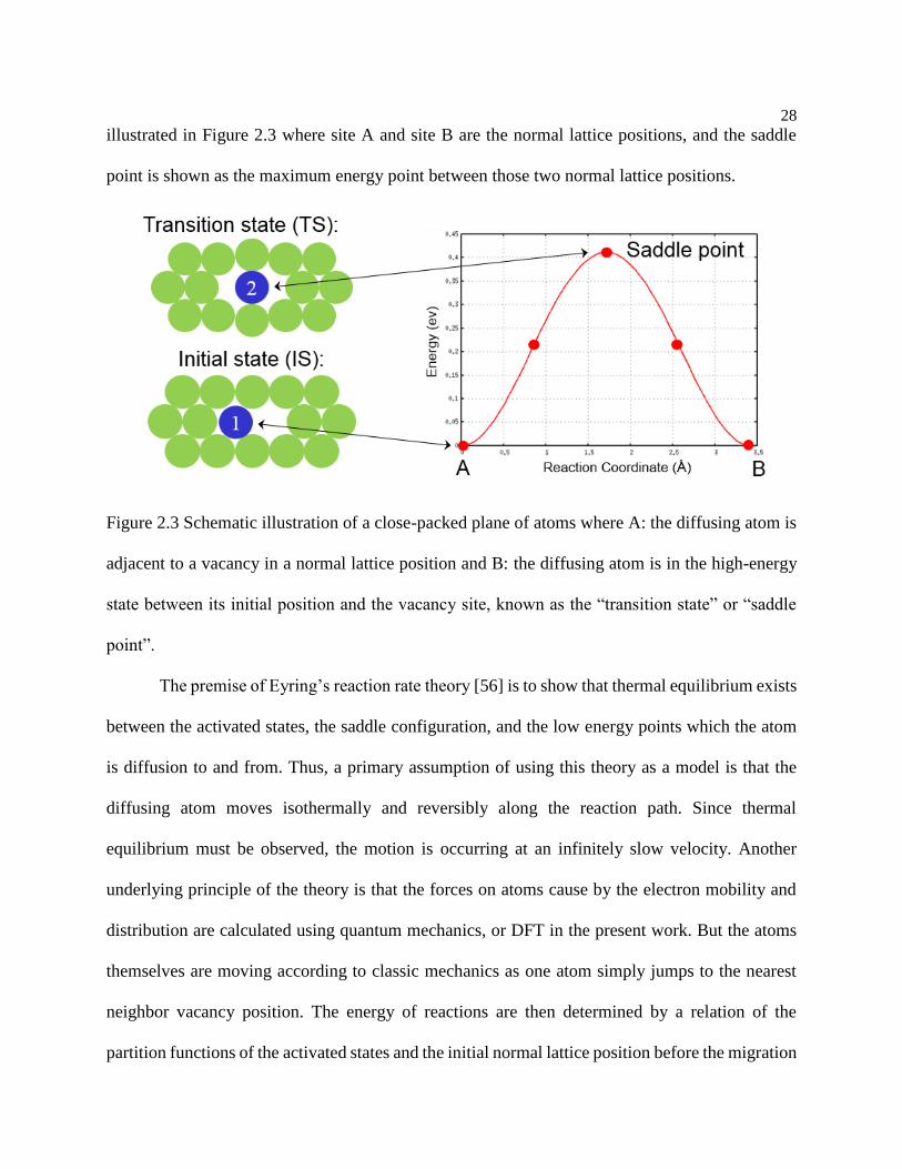
28
illustrated in Figure 2.3 where site A and site B are the normal lattice positions, and the saddle
point is shown as the maximum energy point between those two normal lattice positions.
Figure 2.3 Schematic illustration of a close-packed plane of atoms where A: the diffusing atom is
adjacent to a vacancy in a normal lattice position and B: the diffusing atom is in the high-energy
state between its initial position and the vacancy site, known as the “transition state” or “saddle
point”.
The premise of Eyring’s reaction rate theory [56] is to show that thermal equilibrium exists
between the activated states, the saddle configuration, and the low energy points which the atom
is diffusion to and from. Thus, a primary assumption of using this theory as a model is that the
diffusing atom moves isothermally and reversibly along the reaction path. Since thermal
equilibrium must be observed, the motion is occurring at an infinitely slow velocity. Another
underlying principle of the theory is that the forces on atoms cause by the electron mobility and
distribution are calculated using quantum mechanics, or DFT in the present work. But the atoms
themselves are moving according to classic mechanics as one atom simply jumps to the nearest
neighbor vacancy position. The energy of reactions are then determined by a relation of the
partition functions of the activated states and the initial normal lattice position before the migration

29
began. Glasstone et al. [57] expanded the concept of the reaction rate theory to describe the thermal
activation of solids with a rate constant of k that would represent the jump frequency, w, with a
frequency of vibrations in the system in the direction of the vacancy represented by a velocity, v.
2.4.3 Nudged Elastic Band (NEB) method
As mentioned earlier, the framework of transition state theory involves calculating the
forces acting on the atoms at the various states along the diffusion path using quantum mechanics,
before treating diffusion as classical motion. However, creating a saddle point and allowing all
degrees of freedom to relax using VASP would cause the unstable atom to fall backwards down
the diffusion path and end up in one of the initial or final lattice positions, shown as site A or site
B in Figure 2.3. The saddle configuration is first predicted as the middle of the minimum energy
path between the initial and final equilibrium vacancy configurations, and its final position and
energy are computed using climbing image the nudged elastic band (CI-NEB) method [58][59]
within VASP. The premise of the NEB method involves using a “spring-like” force acting on the
unstable atom while looking at intermediate steps along the diffusion path, called images. In the
present work, one or three images are used to calculate the the forces acting on the saddle
configuration. A 5.0 eV/˚ A2 spring constant was used in all NEB calculations to nudge the image
to the minimum energy path between the initial and final vacancy configurations. Calculations
were allowed to fully relax within the confines of NEB, and the structure was checked to ensure
that local relaxations did not distort the cell or cause reversal of the diffusing atom to one of the
equilibrium vacancy spots. This however, was not the fullest relaxation possible for the saddle
configuration. The usage of the CINEB method will be discussed in the relevant chapters.

30
Chapter 3
First-principles calculations and thermodynamic modeling of Sn-Sr and Mg-Sn-Sr
systems
3.1 Introduction
In recent years, magnesium alloys have generated great interest due to their lightweight,
earth abundance, high specific strength, and good castablity [1]. These properties make Mg alloys
attractive for automotive, aerospace and other light-weight structural applications [3]. Commercial
Mg alloys for automotive applications are mostly Mg-Al based (AZ and AM series) systems,
which offer good room-temperature strength, corrosion resistance, and die castability. However,
these alloys suffer poor creep resistance at elevated temperatures (>125 C) due to the poor thermal
stability of the Mg17Al12 phase, which makes them inadequate for automotive powertrain
applications [60]. Although rare earth elements have been found to greatly improve the creep
performance of Mg alloys [61], the high cost of these alloys prevents their large-scale deployment.
Sn is an abundant and relatively cheap element in comparison with rare earths, which is widely
used in solder and plating industry. As a promising candidate for rare earth-free Mg alloys, Mg-
Sn based alloys have received renewed attention since 2006 due to their potential applications at
elevated temperatures [62–66]. The Mg-Sn system is an age-hardenable system and exhibits good
castability due to the eutectic nature of its phase diagram [65]. The main precipitate phase Mg2Sn
in Mg-Sn based alloys has a melting point of 770 ˚C, which is much higher than that of Mg17Al12
31
phase (462 ˚C) in Mg-Al alloys [67]. These properties make Mg-Sn based alloys a promising Mg
alloy system for automobile powertrain applications at elevated temperatures.
Recent studies showed that the age-hardening response of Mg-Sn based alloys can be
greatly enhanced by alloying additions such as Ca, Na, Si, Zn [62,63,66,68]. The alloying elements
can modify the microstructure of Mg-Sn alloys and yield a finer dispersion of the Mg2Sn
precipitate phase [64]. Therefore, the Mg-Sn alloy with proper alloying additions results a much
larger peak hardness during the aging process [62]. Further rational design of Mg-Sn based alloys
requires accurate knowledge of the thermodynamics of Mg-Sn-X (single additions) and Mg-Sn-
(X-Y) (double additions) systems, which is largely unavailable in the literature [63]. The
CALPHAD (CALculation of PHAse Diagrams) method [11] has proven to be an invaluable
method to model and predict phase equilibria in multi-component materials. Therefore, there is a
pressing need to develop thermodynamic databases of Mg-Sn based alloys based on the
CALPHAD technique [69].
Sr is an important alloying element in Mg alloys. Not only can it reduce the shrinkage and
porosity in die-cast Mg alloys, but also has a grain refinement effect on some Mg alloys systems
like AZ31 and AZ91 [70]. Recent study by Liu et al. [71] showed that an optimum addition of Sr
in Mg-5 wt% Sn alloy can improve the mechanical properties as well as the thermal stability of
Mg-Sn alloys. A rod-shaped or bone-shaped ternary phase MgSnSr is also observed in their study,
which serves as the main straddle on the grain boundaries, preventing grain boundary sliding [71].
A recent study [72] also found that MgSnSr phase could impede crack propagation at grain
boundaries at elevated temperatures. However, thermodynamic modeling of the Mg-Sn-Sr ternary
system has not been reported. In order to study the phase relations and precipitation sequence in
32
Mg-Sn-Sr alloys for improved creep resistance, a complete thermodynamic description of the Mg-
Sn-Sr system needs to be achieved, which is the main goal of the present study.
Several Sn-containing binary systems, such as Sn-Ca [73], Sn-Ce [74], Sn-Na [75] and Sn-
Sr [76] systems, exhibit short-range ordering in the liquid phase. Consequently, there are steep
liquidus and many stable intermetallic compounds with much higher melting point than their
constituent elements in these binary phase diagrams. Traditional modeling strategy of these
compounds using the Neumann-Kopp approximation yields artificial kinks in the heat capacity
descriptions at the melting point of the constituent elements. First-principles phonon calculations
and Debye model [35] are used in the present work to directly predict the finite-temperature
thermodynamic properties of the intermetallic compounds in the Sn-Sr and Mg-Sn-Sr systems,
which provide data for robust CALPHAD modeling and resolve the heat capacity artifact problem
due to the Neumann-Kopp approximation. The Sn-Sr binary system is re-modeled in the present
work and compared with Zhao et al.’s previous modeling work [77]. Thermodynamic descriptions
of the Mg-Sn [78] and Mg-Sr [79] systems are taken from the literature. Combining the
thermodynamic models of three constituent binary systems and the ternary MgSnSr compound,
the thermodynamic description of the Mg-Sn-Sr ternary system is obtained, and phase relations in
the ternary system are predicted.
3.2 Literature Review
In this section, we first briefly discuss the thermodynamic modeling of the Mg-Sn and Mg-
Sr systems. The experimental information and Zhao et al.’s thermodynamic modeling work of the
Sn-Sr system [77] are then carefully reviewed.
33
Mg-Sn binary system
Thermodynamic modeling of the Mg-Sn system was first reported by Fries and Lukas [80]
and subsequently modified by Kozlov et al. [78]. The liquid phase was modeled using the associate
solution model with Mg2Sn as the associate. Afterwards, Meng et al. [81] re-modeled the Mg-Sn
system using the same model as Fries and Lukas [80], while Jung et al. [82] and Ghosh et al. [83]
modeled the Mg-Sn system with the liquid phase described by the modified quasichemical model.
The thermodynamic parameters and predicted phase diagrams of the Mg-Sn system from Meng et
al. [81] are similar to those of Kozlov et al. [78]. Considering the compatibility of thermodynamic
models in terms of the compound energy formalism, the modeling of Kozlov et al. [78] is used in
the present work. Figure 3.1 shows the calculated phase diagram for the Mg-Sn system using the
data sets in Ref. [78].
Mg-Sr binary system
Zhong et al. [79] reported the thermodynamic modeling of the Mg-Sr system with the
enthalpies of formation of the compounds from first-principles calculations. Later, Aljarrah and
Medraj [84] re-modeled the system using the modified quasichemical model. Because the
enthalpies of formation of compounds in the Mg-Sr system by Aljarrah and Medraj [84] do not lie
on a convex hull at all, Zhong et al.’s work [79] is considered to be more reliable and thus is used
in the present work. Figure 3.2 shows the calculated phase diagram for the Mg-Sr system using
the data sets in Ref. [79].
Sn-Sr binary system

34
The experimental work on Sn-Sr system is rather scarce. In fact, it was not until the recent
work by Palenzona and Pani [85] that a complete list of intermetallic compounds formed in the
central regions of the phase diagram was determined.
Okamoto [76] briefly reviewed the phase relations and crystallographic data in the Sn-Sr
system. The crystallographic data of solid phases in the Sn-Sr system are shown in Table 3.1. In
1930, Ray [86] first investigated the phase equilibria of the Sn-Sr system in the composition range
of 63-100 at% Sn using thermal analysis and optical microscopy. Two compounds, Sn5Sr and
Sn3Sr, were considered to be stable. In 1981, Marshall and Chang [87] measured the phase
relations from 65 to 100 at% Sn using various techniques such as differential thermal analysis
(DTA), micro-probe analysis, metallography, and X-ray diffractography (XRD). They found that
the stoichiometry of compound Sn5Sr reported by Ray [86] should be Sn4Sr instead. The phase
relations at <65 at% Sn in the Sn-Sr system were further studied by Widera and Schafer [88] using
DTA and XRD. Their work showed the existence of the Sn3Sr, SnSr, Sn3Sr5, and SnSr2 phases.
Based on the work from Marshall and Chang [87] and Widera and Schafer [88], Massalski [89]
proposed a Sn-Sr phase diagram over the whole composition range in 1990. He believed that there
could be allotropic transitions for SnSr and SnSr2 phases. In 2001, Zürcher et al. [90] synthesized
and characterized the new binary Sn5Sr3 phase. They found that Sn5Sr3 melts peritectically at 810
˚C to SnSr and liquid, and SnSr melts congruently at 910 ˚C. Later, Hoffmann [91] extensively
studied the phase relations of the Sn-Sr system from 57 to 88.4 at% Sn by means of DTA. The
work of Hoffmann [91] and the earlier work by Zürcher et al. [90] both indicated that the Sn5Sr3
compound should be stable in the Sn-rich side.
Recently, Palenzona and Pani [85] re-investigated the whole composition range of the Sn-
Sr system by means of DTA, XRD, and optical microscopy. Their experimental results [85] clearly
35
ruled out the possibility of allotropic transitions for SnSr and SnSr2 phases, which is different
from the phase diagram proposed by Massalski [89] and the experimental result of Widera and
Schafer [88]. Besides, most of the liquidus and invariant reaction temperatures by Palenzona and
Pani [85] agree reasonably well with the data assessed by Massalski and with the experimental
work of Hoffmann [91]. For the sake of consistency, the experimental phase diagram data from
Refs. [87,88,90,91] are not used in the present thermodynamic modeling, only the most recent
data from Palenzona and Pani [85] are used in the present work.
Compared to the phase equilibrium data, thermochemical data in the Sn-Sr system is even
scarcer. Using the heat of reaction of SnSr2+4.42HCl=2SrCl2+0.21SnCl2+2.21H2+0.79Sn,
Morozova et al. [92] estimated the enthalpy of formation at 25 ˚C for SnSr2 to be -115.42 kJ/mol-
atom. This value is not considered in the present modeling as it is in serious conflict with the
enthalpy of formation for SnSr2 predicted from first-principles. King and Kleppa [93], Guadagno
et al. [94] and Esin et al. [95] measured the partial enthalpies of Sr in liquid Sn at 704 K, 775 K,
and 1773 K respectively. Their data are consistent. Therefore, all of their measured partial
enthalpies data are used in the present modeling. The partial enthalpy of dissolution of Sr in liquid
Sn is expressed as Δ𝐻𝑆𝑟∞ = 𝜇𝑆𝑟 − 𝑇
𝑑𝜇𝑆𝑟
𝑑𝑇 in Thermo-Calc [36]. Esin et al. [95] also measured the
enthalpy of mixing in liquid phase at 1773 K for the Sn-Sr system from 0 to 50 at% Sr.
Unfortunately, using their enthalpy of mixing data yields extremely unstable liquid phase and
unreasonably high liquidus in the present modeling. Therefore, the enthalpy of mixing in liquid
data from Esin et al. [95] is not used in the present work.
Mg-Sn-Sr ternary system
36
There are no experimental data for the Mg-Sn-Sr ternary system except the existence of
the MgSnSr compound. Eisenmann et al. [96] synthesized the MgSnSr compound and determined
its crystal structure to be orthorhombic anti-PbCl2 type, which is similar to the crystal structure of
MgSnCa compound reported in the Mg-Sn-Ca system [78]. It is hypothesized in this work that
there may be a solid solution between MgSnSr and SnSr2 compound as their crystal structures
share the same space group Pnma.
3.3 Calculation and modeling details
3.3.1 First-principles calculations
First-principles calculations based on the density functional theory were employed to
predict the finite-temperature thermodynamic properties of phases of interest. The Vienna ab initio
simulation package (VASP) 5.2.12 [49] was used to perform the first-principles calculations within
the generalized gradient approximation (GGA) of Perdew, Burke, and Ernzerhof (PBE) [46]. The
electronic states 3s2, 5s25p2, and 5s2 were considered as valence states for Mg, Sn, and Sr,
respectively. The ion-electron interactions were described by the projector augmented wave
method (PAW) [97] with an energy cutoff of 350 eV for all the structures. The cell volume, shape
and atomic arrangements were fully relaxed using the Methfessel-Paxton method and at least 5000
k-points per reciprocal atom based on the Monkhorst-Pack scheme for the Brillouin-zone sampling
was used. For hcp Mg, the Gamma centered scheme was used for the Brillouin-zone sampling. A
detailed list of the k-mesh setting for each compound can be found in Table 3.3.
Among the six intermetallic compounds in the Sn-Sr system, two compounds, SnSr and
SnSr2, melt congruently, thus defining in great part the topology of the phase diagram. The Sn3Sr5

37
compound also has very high melting point. Therefore, their thermodynamic properties are of great
importance in the present thermodynamic modeling. Due to the scarcity and likely inaccuracies of
the thermochemical data in this system, it is thus necessary to attempt to describe the finite
temperature thermodynamic properties of these compounds through first-principles. In the case of
perfectly ordered, defect-free non-magnetic crystalline metallic phases, the major contributions to
the free energy come from the vibrational (phonon) and thermal electronic excitations [98].
Using the quasi-harmonic approach [35,98], the Helmholtz free energy of a stoichiometric
phase as a function of volume V and temperature T, 𝐹(𝑉, 𝑇), is given by [98]
𝐹(𝑉, 𝑇) = 𝐸0(𝑉) + 𝐹𝑣𝑖𝑏(𝑉, 𝑇) + 𝐹𝑒𝑙𝑒(𝑉, 𝑇) (3.1)
where 𝐸0(𝑉) is the 0 K total energy, 𝐹𝑣𝑖𝑏(𝑉, 𝑇) the vibrational free energy of the lattice ions, and
𝐹𝑒𝑙𝑒(𝑉, 𝑇) the thermal electronic contribution to the free energy. At zero pressure, the Helmholtz
energy of the system equals to the Gibbs energy. In the present work, 𝐸0(𝑉) is obtained via first-
principles calculations for each phase in the system. For the MgSnSr compound, 𝐹𝑣𝑖𝑏(𝑉, 𝑇) is
obtained using both the quasi-harmonic phonon calculations based on the supercell approach and
the empirical Debye-Grüneisen model [35], showing a good agreement. The phonon dispersion
relations with phonon density of states of the MgSnSr compound are shown in Figure 3.3. It shows
that the MgSnSr compound is dynamically stable at 0 K since there are no negative phonon
frequencies from the phonon calculation. With the Debye-Gruneisen model validated by phonon
calculations, 𝐹𝑣𝑖𝑏(𝑉, 𝑇) for other compounds are obtained only from the Debye-Gruneisen model
for the sake of simplicity and efficiency. Since the elements of interest in the present work are
metallic, the thermal electronic contribution to the Helmholtz energy is included due to electronic
excitations at high temperatures around the Fermi level. The thermal electronic contribution to

38
Helmholtz energy is based on the electronic Density of States (DOS) using Fermi-Dirac statistics
[98].
In the quasi-harmonic phonon calculations, based on the partition function of lattice
vibration, the vibrational contribution to Helmholtz free energy can be expressed as
𝐹𝑣𝑖𝑏(𝑉, 𝑇) = 𝑘𝐵𝑇 ∫ 𝑙𝑛 [2 𝑠𝑖𝑛ℎħ𝜔
2𝑘𝐵𝑇]
∞
0
𝑔(𝜔, 𝑉)𝑑𝜔 (3.2)
where ħ is the reduced Planck constant, ω the phonon frequency, and 𝑔(𝜔, 𝑉) is the phonon DOS
at frequency 𝜔 and volume V. The phonon properties of pure Mg, Sn, Sr, SnSr2, and MgSnSr
compounds were studied by the supercell approach as implemented in the Yphon code [48]. With
the obtained phonon DOS at four different volumes in the present work for Mg, Sn, Sr, SnSr2, and
MgSnSr compounds, the Helmholtz free energies are calculated based on the quasi-harmonic
approximation and used in the CALPHAD modeling.
Although quasi-harmonic phonon calculation proves to be an accurate method to obtain
the finite temperature thermodynamic properties, it is computationally very demanding, especially
for structures with large unit cell. Therefore, for the compounds Sn4Sr, Sn3Sr, Sn3Sr5, SnSr, and
Sn5Sr3, we use quasi-harmonic Debye model. In the quasi-harmonic Debye model [35], the
vibrational contribution to Helmholtz energy is described as
𝐹𝑣𝑖𝑏(𝑉, 𝑇) =9
8𝑘𝐵Θ𝐷(𝑉) + 𝑘𝐵𝑇 [3 ln (1 − 𝑒−
ΘD(V)T ) − 𝐷 (
ΘD(𝑉)
T)] (3.3)
where Θ𝐷 is the Debye temperature, 9
8𝑘𝐵Θ𝐷(𝑉) the zero-point energy at 0 K, and 𝑘𝐵 the
Boltzmann’s constant. The Debye function, 𝐷(𝑥), is defined as follows:

39
𝐷(𝑥) =3
𝑥3∫
𝑧3𝑑𝑧
𝑒𝑧 − 1
𝑥
0
(3.4)
In order to solve (3.3), the Debye temperature, ΘD, must be calculated. In the present work,
the Debye-Grüneisen approximation is used to describe ΘD as follows [35]:
ΘD = 𝑠𝐴𝑉01/6
(𝐵0
𝑀)
1/2
(𝑉0
𝑉)
𝛾
(3.5)
where A is a constant, representing (6𝜋2)1/3ℎ/𝑘𝐵, 𝑉0 the ground state volume, 𝑀 the atomic mass,
𝛾 the Gruneisen parameter, 𝐵0 the bulk modulus, and 𝑠 a parameter that scales the Debye
temperature. Although based on a survey of 14 nonmagnetic cubic metals, Moruzzi et al. [53]
showed that a scaling factor of s=0.617 well reproduces the bulk modulus of those 14 metals,
s=0.617 may not be suitable for the intermetallic phases in the present Mg-Sn-Sr system since the
scaling factor is known to be related to the anisotropy of sound velocity in solids. Finally the
Grüneisen parameter is defined as 𝛾 = (1
2) (1 + 𝐵0
′ ) − 𝑥, where 𝐵0′ is the first derivative of the
bulk modulus with respect to pressure, and x is 1 for temperatures below the Debye temperature
and 2/3 for temperatures above the Debye temperature. In the present work, the high temperature
value, x=2/3, is used because the data at high temperature will have a great influence on the
thermodynamic properties in the CALPHAD modeling. Since there are no experimental data for
Debye temperature of the binary intermetallic compounds in Sn-Sr system, in the present work we
perform a two-order polynomial fitting of the Debye temperatures for Sn-Sr compounds using the
predicted three Debye temperatures (Sn, Sr, and SnSr2) from phonon DOS’s (see Table 3.3),
ΘD = −86.447𝑥2 + 73.61𝑥 + 159.17 (3.6)
40
where 𝑥 is the mole fraction of Sr. Hence the Debye temperatures for other Sn-Sr compounds are
obtained and given in Table 3.3.
A four-parameter Birch-Murnaghan equation of state (EOS) [51] is adopted herein to fit
𝐸0(𝑉), represented as
𝐸(𝑉) = 𝑎 + 𝑏𝑉−2/3 + 𝑐𝑉−4/3 + 𝑑𝑉−2 (3.7)
Additionally, our experiences show that for metallic systems, the EOS used in the present
work has a lower fitting error [35]. The EOS thus obtained is used to calculate the parameters
needed in the Debye model.
For an ordered phase in the Mg-Sn-Sr system, the enthalpy of formation, Δ𝐻𝑓 , is
determined from:
∆𝐻𝑓
𝑀𝑔𝑥𝑆𝑛𝑦𝑆𝑟𝑧 = 𝐻(𝑀𝑔𝑥𝑆𝑛𝑦𝑆𝑟𝑧) −𝑥
𝑥+𝑦+𝑧𝐻(𝑀𝑔) −
𝑦
𝑥+𝑦+𝑧𝐻(𝑆𝑛) −
𝑧
𝑥+𝑦+𝑧𝐻(𝑆𝑟) (3.8)
where H’s are enthalpies from the finite temperature first-principles Debye or phonon calculations,
and the reference states for compounds are set as hcp (hexagonal closed packed) for Mg, fcc (face-
centered cubic) for Sr, and bct (body-centered tetragonal) for Sn, respectively, namely, the stable
structures of these pure elements at the temperature of 298.15 K and the pressure of 1 bar.
The dilute enthalpies of formation of solid solution phases fcc and bct in the Sn-Sr system
are calculated from 0 K first-principles calculations using a 32-atom supercell. For example the
dilute enthalpy of formation in bct phase is calculated using the following equation:
∆𝐻𝑓𝑑𝑖𝑙𝑢𝑡𝑒 = 𝐻(𝑆𝑛31𝑆𝑟 𝑏𝑐𝑡) − 31𝐻(𝑆𝑛 𝑏𝑐𝑡) − 𝐻(𝑆𝑟 𝑓𝑐𝑐) (3.9)

41
3.3.2 CALPHAD modeling
The Gibbs energy functions of pure Mg, Sn and Sr are taken from the SGTE (Scientific
Group Thermodata Europe) pure element database [37] as is implemented in the PURE4 database
in Thermo-Calc [36]. The intermetallic compounds, SnSr2, Sn3Sr5, SnSr, Sn5Sr3, Sn3Sr and Sn4Sr
and, MgSnSr, are modeled in the present work. The liquid phase is modeled using an associate
solution model to account for its short-range order behavior.
Thermodynamic models
In the present work, the SnSr2, Sn3Sr5, SnSr, Sn5Sr3, Sn3Sr, Sn4Sr, and MgSnSr phases are
treated as stoichiometric compounds. The MgSnSr and SnSr2 compounds can be seen as two
endmembers of a solid solution SnSr2-xMgx, which will be discussed later in this section. The Gibbs
energy of the intermetallic compound phases are described as:
𝐺𝑀𝑔𝑥𝑆𝑛𝑦𝑆𝑟𝑧 − 𝐻𝑆𝐸𝑅 = 𝑎 + 𝑏𝑇 + 𝑐𝑇𝑙𝑛(𝑇) + 𝑑𝑇2 + 𝑒𝑇−1 + 𝑓𝑇3 (3.10)
where a, b, c, d, e and f are model parameters determined from free energy calculated from
the finite-temperature first-principles methods described above. 𝐻𝑆𝐸𝑅 is the stable element
reference (SER) state that refers to the enthalpies of hcp-Mg, fcc-Sr and bct-Sn at 298.15 K and 1
bar.
In the binary Mg-Sn and Sn-Sr systems, the liquid phase is modeled using the associate
solution model with Mg2Sn and SnSr2 phases as the associates, respectively. Accordingly, the
liquid phase in the present ternary system is described using the associate solution model as follows
42
𝐺𝑚𝐿 (𝑇, 𝑦𝑖) = ∑ 𝑦𝑖 𝐺°
𝑖𝐿(𝑇)
5
𝑖=1
+ 𝑅𝑇 ∑ 𝑦𝑖𝑙𝑛𝑦𝑖
5
𝑖=1
+ ∑ ∑ 𝑦𝑖𝑦𝑗 ∑ 𝐿𝑖,𝑗𝑣,𝐿(𝑦𝑖 − 𝑦𝑗)𝑣
𝑛
𝑣=0
5
𝑗<𝑖
4
𝑖=1
(3.11)
where R is the gas constant, 𝑦𝑖 is the mole fraction of specie i in the liquid phase, 𝑖 or 𝑗
represents any of the five species, Mg, Sn, Sr, Mg2Sn, and SnSr2. In (3.11), the parameters
𝐺°𝑀𝑔𝐿 (𝑇), 𝐺°
𝑆𝑛𝐿 (𝑇) and 𝐺°
𝑆𝑟𝐿 (𝑇) represent the Gibbs energies of pure Mg, Sn and Sr liquid,
respectively, taken from the SGTE compilation [37]. 𝐺°𝑀𝑔2𝑆𝑛𝐿 (𝑇) represents the Gibbs energy of
the Mg2Sn associate and is adopted from Ref. [78]. 𝐿𝑖,𝑗𝑣,𝐿
is the 𝑣th interaction parameter between
the species i and j in the liquid phase, 𝐿𝑖,𝑗𝑣,𝐿 = 𝐴𝑣,𝐿 + 𝐵𝑣,𝐿𝑇 with 𝐴 and 𝐵 being the model
parameters to be evaluated.
The Gibbs energy of the SnSr2 associate is given by
𝐺°𝑆𝑛𝑆𝑟2
𝐿 =1
3𝐺°
𝑆𝑛𝐿 +
2
3𝐺°
𝑆𝑟𝐿 + 𝐴 + 𝐵 ∙ 𝑇 + 𝐶 ∙ 𝑇𝑙𝑛𝑇 (3.12)
The parameters 𝐴 , 𝐵 , and 𝐶 are modeled in the present work with the experimental
thermochemical and phase equilibrium data related to the liquid phase.
The solid solution (ss) phase is described by the disordered substitutional solution model
as given by
𝐺𝑚𝑠𝑠 = ∑ 𝑥𝑖 𝐺°
𝑖𝑠𝑠
3
𝑖=1
+ 𝑅𝑇 ∑ 𝑥𝑖𝑙𝑛𝑥𝑖
3
𝑖=1
+ ∑ ∑ 𝑥𝑖𝑥𝑗 ∑ 𝐿𝑖,𝑗𝑣,𝑠𝑠(𝑥𝑖 − 𝑥𝑗)𝑣
𝑛
𝑣=0
3
𝑗>𝑖
2
𝑖=1
(3.13)
where 𝑥𝑖 are the molar fractions of i=Mg, Sn and Sr. 𝐺°𝑖𝑠𝑠(𝑇) is the Gibbs energies of pure
Mg, Sn and Sr in hcp state, which are also taken from the SGTE lattice stability database [37]. 𝐿𝑖,𝑗𝑣,𝐿
is the 𝑣th interaction parameter between the species i and j in the hcp solid solution phase. Similarly,

43
𝐿𝑖,𝑗𝑣,𝑠𝑠 = 𝐴𝑣,𝑠𝑠 + 𝐵𝑣,𝑠𝑠𝑇 with 𝐴 and 𝐵 being the model parameters to be evaluated. In the present
work, we modeled the hcp, fcc, bct solid solution phases. The model parameters 𝐴 in fcc and bct
phases are determined using the dilute enthalpies of formation calculated using first-principles, as
is shown in Figure 3.7.
In the Mg-Sn-Ca system, which is similar to the Mg-Sn-Sr system, the “ternary compound”
MgSnCa is actually found to be the ternary solid solution of Ca2Sn [78]. In the Mg-Sn-Ca
thermodynamic modeling work by Kozlov et al. [78], the MgSnCa and Ca2Sn phases were
modeled as a ternary solid solution SnCa2-xMgx using a sublattice model (Sn)(Ca)(Ca,Mg) which
terminates at the composition x=1, i.e. SnCaMg. Meanwhile, the crystal structures of MgSnSr and
SnSr2 phases share the same Pnma space group. Due to the similarity between the Mg-Sn-Ca and
Mg-Sn-Sr systems, we also treat MgSnSr and SnSr2 phases as a ternary solid solution SnSr2-xMgx
in the present work using a sublattice model (Sn)(Sr)(Sr,Mg). The two endmembers 𝐺𝑆𝑛:𝑆𝑟:𝑀𝑔𝑆𝑛𝑆𝑟2−𝑥𝑀𝑔𝑥
and 𝐺𝑆𝑛:𝑆𝑟:𝑆𝑟𝑆𝑛𝑆𝑟2−𝑥𝑀𝑔𝑥 in the sublattice model correspond to the free energies of MgSnSr and SnSr2
compounds, respectively, which are obtained by finite temperature first-principles calculations.
Meanwhile, a negative interaction parameter 𝐿0𝑀𝑔2𝑆𝑛,𝑆𝑛𝑆𝑟2
𝐿𝑖𝑞 = −15000 between two
associate species Mg2Sn and SnSr2 in the liquid phase is added in the present description to avoid
a liquid miscibility gap in the intermediate temperature range. Unfortunately due to lack of
experimental data in the ternary region this negative interaction between two associate species is
not validated, although similar treatment can be found in the thermodynamic description of Mg-
Sn-Ca system between Mg2Sn and Ca2Sn [78]. The remaining ternary thermodynamic description
is obtained via a Redlich-Kister type extrapolation from the binary edge systems combined with
the thermodynamic model of the SnSr2-xMgx solid solution.
44
Modeling procedure
The thermodynamic modeling is performed using the PARROT module of the Thermo-
Calc software [36]. Evaluation of the model parameters in the Sn-Sr system starts with the
intermetallic phases. First, calculated heat capacity values are used to evaluate parameters c, d, e,
f in (3.10) because they are directly related to the heat capacities. The heat capacity curves are
cutoff at a temperature that is about 50K above the melting temperature of each compound [73].
Due to unavailability of data, constant Cp values are assumed above those temperatures, as is
shown in Figure 3.6, and the parameters a, b, c above the cutoff temperatures can be determined.
Then these parameters are fixed and the next step is to evaluate the b parameter below the
cutoff temperatures in (3.10) using calculated absolute entropy values at 298 K from first-
principles because it is the only remaining term that has a linear dependence to temperature.
Afterwards the calculated enthalpy of formation values at 298 K are used to evaluate the a
parameter in (3.10).
Once the Gibbs energy expressions for all the stoichiometric compounds are determined,
we moved to model the parameters of the liquid phase. It should be noted that some of the
parameters in intermetallic phases also need to be modified in order to describe the steep liquidus
well. The complete and self-consistent thermodynamic parameters of the Mg-Sn-Sr system are
listed in Table 3.4.
45
3.4 Results and Discussion
In order to validate the reliability of the results from the first-principles calculations for the
Sn-Sr system, the calculated lattice parameters and the enthalpies of formation at 0 K and 300 K
of the stoichiometric compounds and pure elements are compared with the available experimental
data and other theoretical values in Table 3.2. The enthalpies of formation and absolute entropies
of the compounds at 300 K from the quasi-harmonic first-principles calculations and current
CALPHAD modeling are shown in Figure 3.4 and Figure 3.5, respectively, showing good
agreement. It should be noted that the enthalpy of formation of Sn3Sr5 is slightly above the convex
hull between SnSr2 and SnSr compounds, demonstrating that Sn3Sr5 should be metastable at room
temperature. The temperature of the solid-state decomposition reaction (Sn3Sr5 ↔ SnSr + SnSr2)
is predicted to be 712 K.
Figure 3.6 shows comparisons between the first-principles calculations and the CALPHAD
modeling results of heat capacity Cp for all the intermetallic compounds in the Mg-Sn-Sr system.
The fitted curves from CALPHAD are cutoff at a temperature that is about 50 K above the melting
temperature of each compound and constant values are assumed above that temperature. It is noted
that in Figure 3.6 the heat capacities of Sn5Sr3, SnSr, Sn3Sr5, MgSnSr, and Sn4Sr are quite similar
below 600 K except for Sn3Sr.
On the other hand, Zhao et al. [77] used the Neuman-Kopp approximation for the heat
capacities of stoichiometric compounds in their modeling of the Sn-Sr system. This led to artificial
kinks in the heat capacity description of the compounds when the melting point of the compounds
exceeds those of the constituent pure elements. In the present work, the quasi-harmonic Debye
model [35] is used with the inputs from first-principles calculations to directly predict the finite-
temperature thermodynamic properties of the intermetallic phases, avoiding the heat capacity
46
artifacts due to the Neumann-Kopp approximation as is shown in Figure 3.6(b) using the Cp of
SnSr as an example. A cutoff at temperature 50 K above the melting point of each compound has
to be made to the fitted Cp curve to avoid unrealistically high values of Cp above the melting
temperatures of the compounds [73].
As can be shown in Figure 3.7, the dilute enthalpies of formation of solid solution phases
fcc and bct are used to model the mixing behavior in the Sn-Sr system. Using dilute enthalpies of
formation instead of dilute enthalpies of mixing in the present CALPHAD modeling has
advantages because dilute enthalpies of formation is more accurate than dilute enthalpies of mixing
since it bypasses the problem of the discrepancies between CALPHAD and first-principles lattice
stabilities [99]. If enthalpies of mixing from first-principles calculations are used in the modeling,
it may induce large errors and undesirably over-stabilize the solid solution phase. In this work
since the lattice stability of Sr in bct is not available in the PURE4 database [37], we use
G(bct,Sr)=GHSERSR+25000 as the lattice stability of Sr in bct structure, where the enthalpy
difference 25000 J/mol between fcc Sr and bct Sr is calculated from the present first-principles
calculations, and GHSERSR is Gibbs energy function of Sr at the standard reference state from
the PURE4 database.
For the thermodynamic description of the solution phases, since the solubility of Sn in Sr
as well as Sr in Sn is extremely small, dilute enthalpy of formation is sufficient to model the mixing
behavior of the Sn-Sr system. While an accurate thermodynamic description of the solution phase
is not important for reproducing the correct Sn-Sr binary phase diagram due to low solubility, it
will become important when the thermodynamic description of Sn-Sr binary system is extended
to higher order systems, especially the thermodynamic functions of the fcc phase.

47
The Sn-Sr binary phase diagram exhibit several features indicating short-range ordering in
the liquid, such as the steep liquidus and the stable intermetallic phases having higher melting
points than their constituent elements. Recently, Zhao et al. [77] modeled the Sn-Sr system with
the liquid phase described by the random solution model and the excess Gibbs energy in terms of
the liquid phase by Redlich-Kister polynomial. Although they got a reasonably good agreement
with the experimental phase boundary data, the multiple high-order interaction parameters are used
in their work to describe the liquidus around the high-melting-temperature intermetallic
compounds. The liquidus at other compositions are less satisfactory in comparison with
experiments.
In the present work, the liquid phase is modeled using the associate model with SnSr2 as
the associate in the liquid phase. This gives a better physical description of the apparent short-
range order behavior of the liquid phase in the Sn-Sr system, thus yielding more robust parameters.
The short-range order behavior can be further examined by plotting the enthalpy and entropy of
mixing in the liquid phase. As is shown in Figure 3.8, there is a deep valley in the enthalpy and
entropy of mixing in the liquid phase around the composition of the high melting point
intermetallic phase SnSr2. This demonstrates that the short-range ordering in the liquid
significantly decreases the entropy of mixing and thus destabilizes the liquid phase. Figure 3.9
shows the calculated liquid species fractions as a function of Sr concentration. It is noted that
around the mole fraction x(Sr) = 2/3 the dominant species in the liquid phase is the SnSr2 associate,
indicating the strong interactions between the atoms in the liquid at compositions around that of
the SnSr2 phase.
The calculated partial enthalpy of dissolution of Sr in liquid Sn is demonstrated in Figure
3.10. The reference state is pure solid Sr at the given temperature so that the partial enthalpy
48
represents the enthalpy difference for the process of dissolving 1 mol fcc Sr in an infinite amount
of liquid Sn. The calculated value is obtained at x(Sr)=1×10⁻³ which is confirmed to be almost
identical as that calculated at x(Sr)=1×10⁻⁴. Although the results from the present modeling are
slightly higher in value than the experimental data, the calculated value lies in a reasonable range
considering the experimental scatter.
Figure 3.11 shows the calculated Sn-Sr binary temperature-composition phase diagram.
The experimentally measured invariant reactions and liquidus temperatures, shown in Table 3.5,
are well reproduced using the present thermodynamic model. Liquidus projection with isotherms
over the entire composition range is shown in Figure 3.13. The isotherms are given with the
interval of 100˚C. It can be seen that a wide SnSr2-xMgx primary solidification region exists. Figure
3.12 shows the calculated isothermal section of the Mg-Sn-Sr phase diagram at room temperature,
confirming the observation of the MgSnSr ternary phase in the experimental work by Liu et al.
[100], which serves as the main strengthening phase pinning grain boundaries and preventing crack
propogation. Composition of Mg alloys can be tailored based on the calculated isothermal section
so that the beneficial phases Mg2Sn and MgSnSr can exist simultaneously.
Shown in Figure 3.14 is the calculated isopleth (vertical section) between Mg2Sn and
Mg2Sr compositions using the current thermodynamic model. Figure 3.15(a) and (b) show the
calculated solidification paths of two Mg-Sn based alloys with different Sr concentrations using
Scheil simulation module in Thermo-Calc [36]. From Figure 3.15 we can see that different Sr
concentration can change the solidification path of Mg-Sn based alloys and higher Sr concentration
can suppress the formation of Mg2Sn phase. Due to insufficient ternary experimental data, the
thermodynamic description of the Mg-Sn-Sr ternary was obtained primarily by extrapolation from
49
the consitituent binaries. Further experimental works may be needed for the future validation and
refinement of the Mg-Sn-Sr ternary description.
3.5 Conclusions
All the experimental phase diagrams and thermodynamic data of the Sn-Sr and Mg-Sn-Sr
systems available in the literature have been critically reviewed. The finite-temperature
thermodynamic properties for seven stoichiometric compounds (SnSr2, Sn3Sr5, SnSr, Sn5Sr3, Sn3Sr,
Sn4Sr, and MgSnSr) in the Mg-Sn-Sr system are computed by phonon and Debye model with
inputs from the first-principles calculations. It provides robust input thermochemical data for
modeling and avoids the artifact of heat capacity description from the Neumann-Kopp
approximation. The short range behavior in the liquid phase of the Mg-Sn-Sr system is well
described by the associate solution model. A complete set of self-consistent thermodynamic
parameters is obtained based on the literature data and the first-principles calculation results.
Comparisons between the calculated and measured quantities indicate that the selected
experimental information can be satisfactorily accounted for by the present thermodynamic
description. The obtained thermodynamic database and predicted phase diagrams provide a design
map for possible precipitate phases in precipitate-strengthened rare-earth free Mg-Sn based alloys
for light-weight applications.
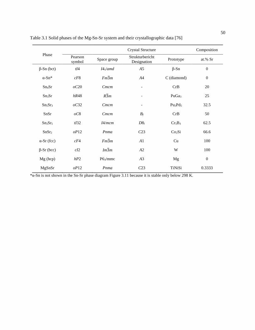
50
Table 3.1 Solid phases of the Mg-Sn-Sr system and their crystallographic data [76]
Phase
Crystal Structure Composition
Pearson
symbol Space group
Strukturbericht
Designation Prototype at.% Sr
β-Sn (bct) tI4 I41/amd A5 β-Sn 0
α-Sn* cF8 Fm3m A4 C (diamond) 0
Sn4Sr oC20 Cmcm - CrB 20
Sn3Sr hR48 R3m - PuGa3 25
Sn5Sr3 oC32 Cmcm - Pu3Pd5 32.5
SnSr oC8 Cmcm Bf CrB 50
Sn3Sr5 tI32 I4/mcm D8l Cr5B3 62.5
SnSr2 oP12 Pnma C23 Co2Si 66.6
α-Sr (fcc) cF4 Fm3m A1 Cu 100
β-Sr (bcc) cI2 Im3m A2 W 100
Mg (hcp) hP2 P63/mmc A3 Mg 0
MgSnSr oP12 Pnma C23 TiNiSi 0.3333
*α-Sn is not shown in the Sn-Sr phase diagram Figure 3.11 because it is stable only below 298 K.

51
Table 3.2 First-principles results of lattice parameters and enthalpies of formation of the intermetallic
compounds in the Mg-Sn-Sr system and their Standard Element Reference (SER) states, hcp-Mg, fcc-Sr
and bct-Sn, along with the available experimental and theoretical data from the literatures. FP=First-
principles.
Phase Method Lattice parameter (Å)
Reference Hf
(kJ/mol-atom) Reference
a b c
hcp-Mg Expa
FP GGA
FP PBE
3.213
3.189
3.219
5.213
5.169
5.099
[101]
[99]
Present work
-
bct-Sn Exp
FP GGA
FP PBE
5.830
5.93
5.933
3.184
3.23
3.202
[101]
[102]
Present work
-
fcc-Sr Exp
FP GGA
FP PBE
6.084
6.000
6.028
[101]
[99]
Present work
-
Sn4Sr Exp
FP GGA
FP PBE
4.625
4.698
4.693
17.383
17.559
17.525
7.070
7.173
7.151
[101]
[77]
Present work
-33.96 (0 K)
-33.693 (0 K)
-33.690 (300 K)
[77]
Present
work
Sn3Sr Exp
FP PBE
6.940
7.002
33.01
33.394
[101]
Present work
-41.74 (0 K)
-41.641 (0 K)
-41.527 (300 K)
[77]
Present
work
Sn5Sr3 Exp
FP GGA
FP PBE
10.560
10.770
10.752
8.590
8.664
8.551
10.901
10.996
10.892
[101]
[77]
Present work
-57.93 (0K)
-57.195 (0K)
-57.226 (300K)
[77]
Present
work
SnSr Exp
FP GGA
FP PBE
5.045
5.112
5.089
12.04
12.187
12.200
4.494
4.525
4.545
[101]
[77]
Present work
-68.88 (0 K)
-67.606 (0 K)
-67.678 (300 K)
[77]
Present
work
Sn3Sr5 Exp
FP GGA
FP PBE
8.565
8.608
8.613
16.261
16.528
16.531
[101]
[77]
Present work
-64.47 (0 K)
-63.018 (0 K)
-63.065 (300 K)
[77]
Present
work
SnSr2 Exp
FP GGA
FP PBE
8.402
8.428
8.426
5.378
5.408
5.407
10.078
10.148
10.167
[101]
[77]
Present work
-63.40 (0 K)
-61.764 (0 K)
-61.930 (300 K)
[77]
Present
work
MgSnSr Exp 8.180
8.221
4.920
4.896
8.750
8.918
[101]
Present work
-56.560 (0 K)
-56.621 (300 K)
Present
work FP PBE aThe experimental lattice parameters are reported at room temperature.

52
Table 3.3 Calculated properties of intermetallic phases and pure elements in Mg-Sn-Sr system at 0K from
first-principles phonon and Debye model in comparison with available experimental data, including volume
(V), bulk modulus (B), first derivative of bulk modulus with respect to pressure (B’), and Debye
temperature (Θ𝐷) together with details of first-principles calculations of each phases, including k-point
mesh for electronic structure calculations, supercell size, and k-point mesh for phonon calculations.
Phase Reference V
(Å3/atom) B (GPa) B’
Θ𝐷 (K) k-point
mesh
electrona
supercell
sizeb
k-point
mesh
phonon Exp fitting phonon
hcp-Mg Present work 22.885 36.180 4.026 322 322
9×9×8 3×3×3 7×7×4 Exp [103] 22.5 36.8 4.3 323
bct-Sn Present work 28.423 47.686 4.864 159 159
20×20×20 3×3×3 2×2×3 Exp [104] 27.055 58 4.8 165
fcc-Sr Present work 54.540 11.443 4.162 146 146
20×20×20 3×3×3 2×2×2 Exp [105] 56.300 11.88 2.41 147
Sn4Sr
Present work
29.588 38.748 4.603 170 - 8×8×7
Sn3Sr 29.695 35.613 5.604 172 - 6×6×6
Sn5Sr3 32.178 32.027 4.416 175 - 6×6×5
SnSr 35.413 32.459 4.530 174 - 11×11×11
Sn3Sr5 38.400 25.730 4.120 171 - 4×4×5
SnSr2 38.730 23.308 3.850 170 170 6×9×5 2×2×2 3×5×2
MgSnSr 30.003 35.607 4.342 256 256 8×8×7 2×2×2 2×3×2
aThe electronic k-point mesh is for primitive unit cell of each phase.
bThe supercell construction for phonon calculation is based on conventional unit cell of each phase.

53
Table 3.4 Thermodynamic parameters of the Mg-Sn-Sr ternary system (in S.I. units)
Phase and model Model parameters Ref.
Liquid,
(Mg,Sn,Sr,Mg2Sn,
SnSr2) associate
solution model, (3.11)
𝐺𝑀𝑔2𝑆𝑛𝐿𝑖𝑞
= 2 ∙ 𝐺°𝑀𝑔𝐿 + 𝐺°
𝑆𝑛𝐿 − 69092.9 + 97.6086 ∙ 𝑇 − 11.0957 ∙ 𝑇
∙ 𝑙𝑛(𝑇)
[78]
𝐺𝑆𝑛𝑆𝑟2
𝐿𝑖𝑞= 𝐺°
𝑆𝑛𝐿 + 2 ∙ 𝐺°
𝑆𝑟𝐿 − 140846.086 + 12.1011 ∙ 𝑇 Present
work
𝐿0𝑆𝑛,𝑆𝑛𝑆𝑟2
𝐿𝑖𝑞= −134258.124
𝐿1𝑆𝑛,𝑆𝑛𝑆𝑟2
𝐿𝑖𝑞= −38456.877
𝐿0𝑀𝑔2𝑆𝑛,𝑆𝑛𝑆𝑟2
𝐿𝑖𝑞= −15000
𝐿0𝑀𝑔,𝑀𝑔2𝑆𝑛𝐿𝑖𝑞
= 6902.76 − 9.22726 ∙ 𝑇 [78]
𝐿0𝑀𝑔,𝑆𝑛𝐿𝑖𝑞
= −31251 + 0.74703 ∙ 𝑇
𝐿0𝑀𝑔2𝑆𝑛,𝑆𝑛𝐿𝑖𝑞
= −8289.15 − 10.0268 ∙ 𝑇
𝐿0𝑀𝑔,𝑆𝑟𝐿𝑖𝑞
= −20857.771 + 6.35745 ∙ 𝑇 [79]
𝐿1𝑀𝑔,𝑆𝑟𝐿𝑖𝑞
= −13008.376 + 4.71516 ∙ 𝑇
Hcp (Mg,Sn,Sr) 𝐿0𝑀𝑔,𝑆𝑛ℎ𝑐𝑝
= −30000 − 3 ∙ 𝑇 [78]
𝐿1𝑀𝑔,𝑆𝑛ℎ𝑐𝑝
= −11293.8 − 4.42051 ∙ 𝑇
𝐿0𝑀𝑔,𝑆𝑟ℎ𝑐𝑝
= 10000 [79]
𝐿0𝑆𝑛,𝑆𝑟ℎ𝑐𝑝
= 50000 Present
work
Fcc (Mg,Sn,Sr) 𝐿0𝑀𝑔,𝑆𝑟𝑓𝑐𝑐
= 20000 [79]
𝐿0𝑆𝑛,𝑆𝑟𝑓𝑐𝑐
= −43803.497
𝐿1𝑆𝑛,𝑆𝑟𝑓𝑐𝑐
= 41065.879
Present
work
Bcc (Mg,Sn,Sr) 𝐿0𝑀𝑔,𝑆𝑟𝑏𝑐𝑐 = 20000 [79]
𝐿0𝑆𝑛,𝑆𝑟𝑏𝑐𝑐 = 50000 Present
work
Bct (Mg,Sn,Sr) 𝐿0𝑆𝑛,𝑆𝑟𝑏𝑐𝑡 = −63355.128
𝐿1𝑆𝑛,𝑆𝑟𝑏𝑐𝑡 = −59395.433
(Mg)2/3(Sn)1/3 𝐺𝑀𝑔2𝑆𝑛 = −31024.2 + 110.918 ∙ 𝑇 − 21.8911 ∙ 𝑇 ∙ 𝑙𝑛(𝑇) − 0.003028
∙ 𝑇2 − 210000 ∙ 𝑇−1
[78]
(Mg)17(Sr)2 𝐺𝑚𝑀𝑔17𝑆𝑟2 = 17 ∙ 𝐺°
𝑀𝑔ℎ𝑐𝑝
+ 2 ∙ 𝐺°𝑆𝑟ℎ𝑐𝑝
− 90038.622 + 14.05441 ∙ 𝑇 [79]
(Mg)38(Sr)9 𝐺𝑚𝑀𝑔38𝑆𝑟9 = 38 ∙ 𝐺°
𝑀𝑔ℎ𝑐𝑝
+ 9 ∙ 𝐺°𝑆𝑟ℎ𝑐𝑝
− 338997.90 + 54.72598 ∙ T
(Mg)23(Sr)6 𝐺𝑚𝑀𝑔23𝑆𝑟6 = 23 ∙ 𝐺°
𝑀𝑔ℎ𝑐𝑝
+ 6 ∙ 𝐺°𝑆𝑟ℎ𝑐𝑝
− 222032.27 + 37.28284 ∙ T
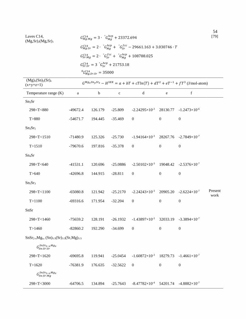
54
Laves C14,
(Mg,Sr)2(Mg,Sr)1 𝐺𝑀𝑔:𝑀𝑔
𝐶14 = 3 ∙ 𝐺°𝑀𝑔ℎ𝑐𝑝
+ 23372.694 [79]
𝐺𝑀𝑔:𝑆𝑟𝐶14 = 2 ∙ 𝐺°
𝑀𝑔ℎ𝑐𝑝
+ 𝐺°𝑆𝑟𝑓𝑐𝑐
− 29661.163 + 3.030746 ∙ 𝑇
𝐺𝑆𝑟:𝑀𝑔𝐶14 = 2 ∙ 𝐺°
𝑆𝑟𝑓𝑐𝑐
+ 𝐺°𝑀𝑔ℎ𝑐𝑝
+ 108788.025
𝐺𝑆𝑟:𝑆𝑟𝐶14 = 3 𝐺°
𝑆𝑟ℎ𝑐𝑝
+ 21753.18
𝐿0𝑀𝑔,𝑆𝑟:𝑆𝑟𝐶14 = 35000
(Mg)x(Sn)y(Sr)z
(x+y+z=1) 𝐺𝑀𝑔𝑥𝑆𝑛𝑦𝑆𝑟𝑧 − 𝐻𝑆𝐸𝑅 = 𝑎 + 𝑏𝑇 + 𝑐𝑇𝑙𝑛(𝑇) + 𝑑𝑇2 + 𝑒𝑇−1 + 𝑓𝑇3 (J/mol-atom)
Temperature range (K) a b c d e f
Sn3Sr
Present
work
298<T<880 -49672.4 126.179 -25.809 -2.24295×10⁻³ 28130.77 -1.2473×10⁻⁶
T>880 -54671.7 194.445 -35.469 0 0 0
Sn3Sr5
298<T<1510 -71480.9 125.326 -25.730 -1.94164×10⁻³ 28267.76 -2.7849×10⁻⁷
T>1510 -79670.6 197.816 -35.378 0 0 0
Sn4Sr
298<T<640 -41531.1 120.696 -25.0886 -2.50102×10⁻³ 19048.42 -2.5376×10⁻⁷
T>640 -42696.8 144.915 -28.811 0 0 0
Sn5Sr3
298<T<1100 -65080.8 121.942 -25.2170 -2.24243×10⁻³ 20905.20 -2.6224×10⁻⁷
T>1100 -69316.6 171.954 -32.204 0 0 0
SnSr
298<T<1460 -75659.2 128.191 -26.1932 -1.43897×10⁻³ 32033.19 -3.3894×10⁻⁷
T>1460 -82860.2 192.290 -34.699 0 0 0
SnSr2-xMgx, (Sn)1/3(Sr)1/3(Sr,Mg)1/3
𝐺𝑆𝑛:𝑆𝑟:𝑆𝑟𝑆𝑛𝑆𝑟2−𝑥𝑀𝑔𝑥
298<T<1620 -69695.8 119.941 -25.0454 -1.60872×10⁻³ 18279.73 -1.4661×10⁻⁷
T>1620 -76381.9 176.635 -32.5622 0 0 0
𝐺𝑆𝑛:𝑆𝑟:𝑀𝑔𝑆𝑛𝑆𝑟2−𝑥𝑀𝑔𝑥
298<T<3000 -64706.5 134.894 -25.7643 -8.47782×10⁻⁴ 54201.74 -4.8882×10⁻⁷
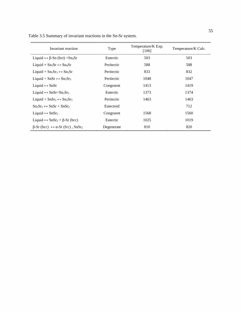
55
Table 3.5 Summary of invariant reactions in the Sn-Sr system.
Invariant reaction Type Temperature/K Exp.
[106] Temperature/K Calc.
Liquid ↔ β-Sn (bct) +Sn4Sr Eutectic 503 503
Liquid + Sn3Sr ↔ Sn4Sr Peritectic 588 588
Liquid + Sn5Sr3 ↔ Sn3Sr Peritectic 833 832
Liquid + SnSr ↔ Sn5Sr3 Peritectic 1048 1047
Liquid ↔ SnSr Congruent 1413 1419
Liquid ↔ SnSr+Sn3Sr5 Eutectic 1373 1374
Liquid + SnSr2 ↔ Sn3Sr5 Peritectic 1463 1463
Sn3Sr5 ↔ SnSr + SnSr2 Eutectoid 712
Liquid ↔ SnSr2 Congruent 1568 1560
Liquid ↔ SnSr2 + β-Sr (bcc) Eutectic 1025 1019
β-Sr (bcc) ↔ α-Sr (fcc) , SnSr2 Degenerate 810 820

56
Figure 3.1. Mg-Sn binary phase diagram calculated from the data sets given in Ref. [78].
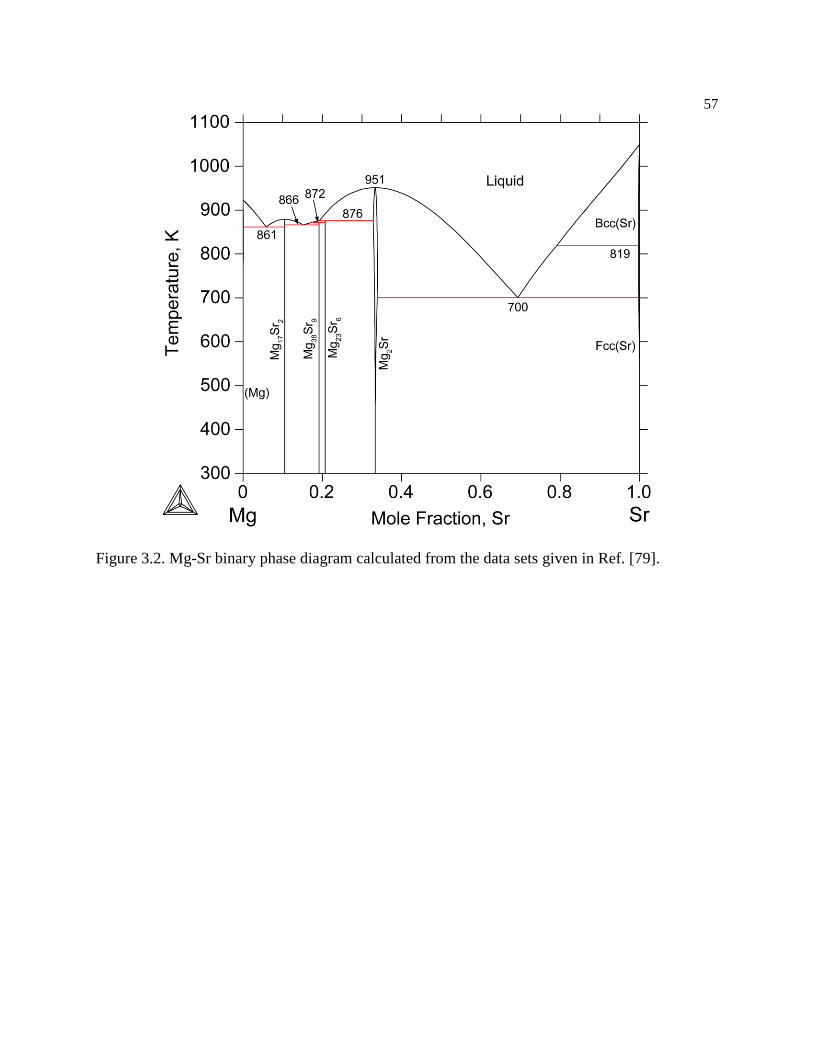
57
Figure 3.2. Mg-Sr binary phase diagram calculated from the data sets given in Ref. [79].
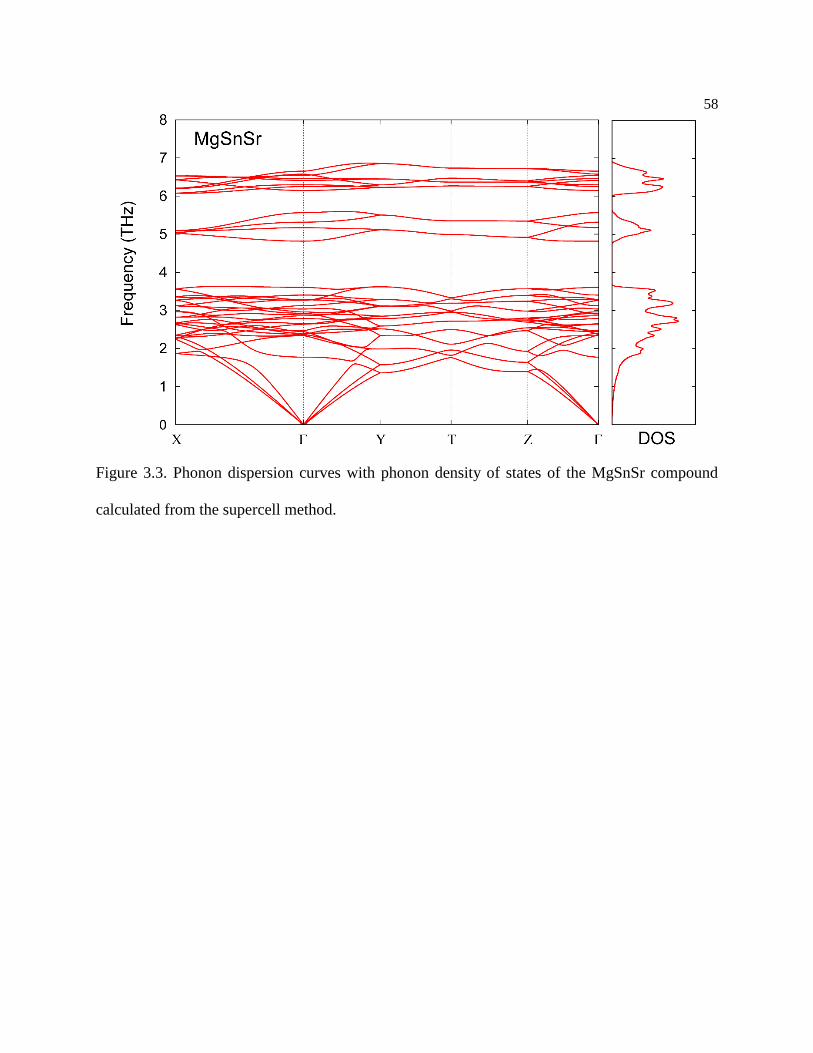
58
Figure 3.3. Phonon dispersion curves with phonon density of states of the MgSnSr compound
calculated from the supercell method.
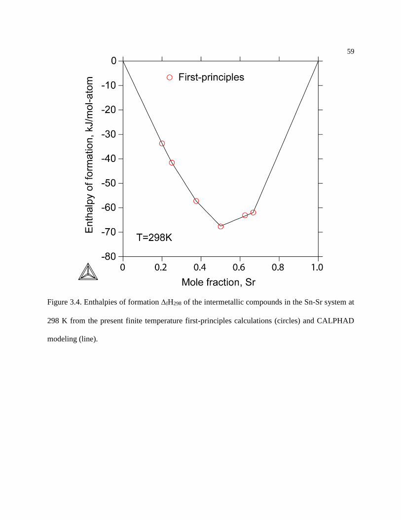
59
Figure 3.4. Enthalpies of formation fH298 of the intermetallic compounds in the Sn-Sr system at
298 K from the present finite temperature first-principles calculations (circles) and CALPHAD
modeling (line).

60
Figure 3.5. Absolute entropies S298 for the stable solid phases in the Sn-Sr system at 298K from
the present finite temperature first-principles calculations (circles) and CALPHAD modeling (line).

61
(a)
(b)

62
Figure 3.6. (a) Temperature dependence of heat capacities for all the stoichiometric compounds in
the Mg-Sn-Sr system from CALPHAD modeling and first-principles Debye model by solid and
dashed lines, respectively. (b) Heat capacity of SnSr from the present CALPHAD modeling in
comparison with that obtained from the Neumann-Kopp approximation. The kink corresponds to
the melting point of β-Sn.

63
Figure 3.7, Enthalpy of formation of the solid solution phases from the present CALPHAD
modeling (lines) together with the dilute enthalpies of formation from first-principles (circles).
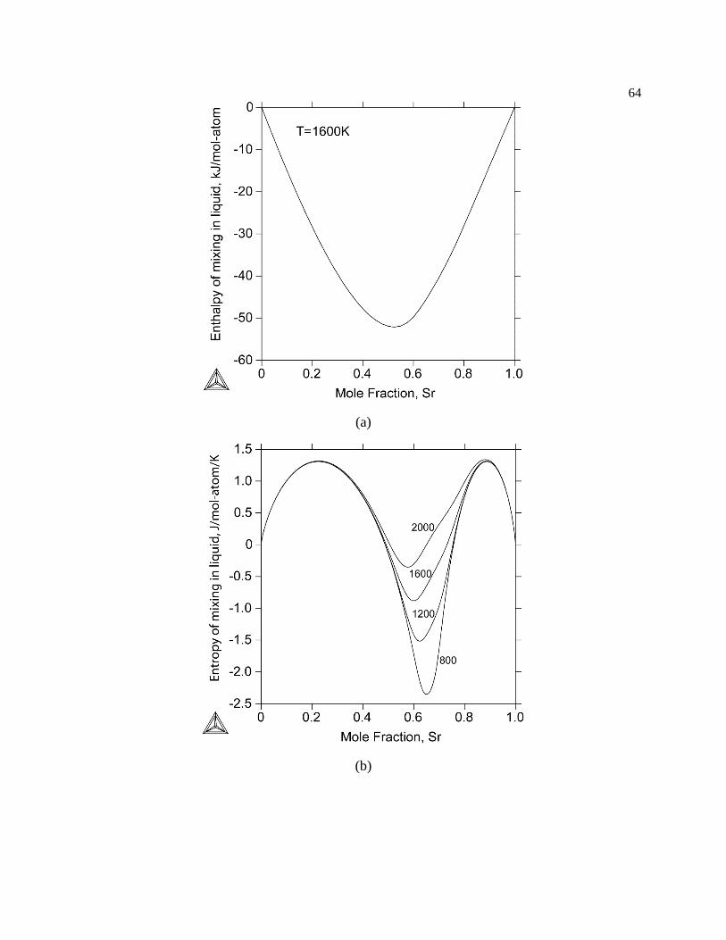
64
(a)
(b)

65
Figure 3.8. (a) Calculated enthalpy of mixing in the liquid at 1600 K. (b) Calculated entropy of
mixing in the liquid at 2000, 1600, 1200, and 800 K from the present CALPHAD modeling. The
liquid phase at 1200 and 800 K is metastable.

66
Figure 3.9. Mole fractions of species in liquid as a function of total Sr concentration at 1600 K,
calculated from the present CALPHAD modeling.
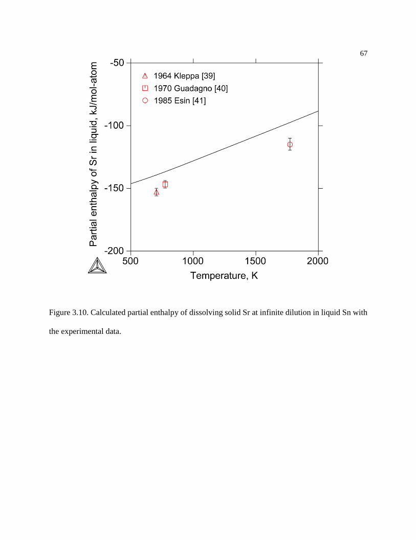
67
Figure 3.10. Calculated partial enthalpy of dissolving solid Sr at infinite dilution in liquid Sn with
the experimental data.
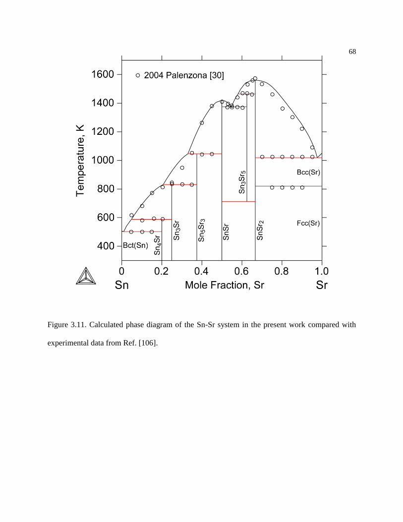
68
Figure 3.11. Calculated phase diagram of the Sn-Sr system in the present work compared with
experimental data from Ref. [106].
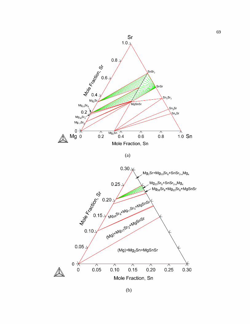
69
(a)
(b)

70
Figure 3.12. Calculated isothermal sections of the Mg-Sn-Sr phase diagram at 298.15 K: (a)
isothermal section of the whole composition range and (b) an enlarged isothermal section at Mg-
rich corner.
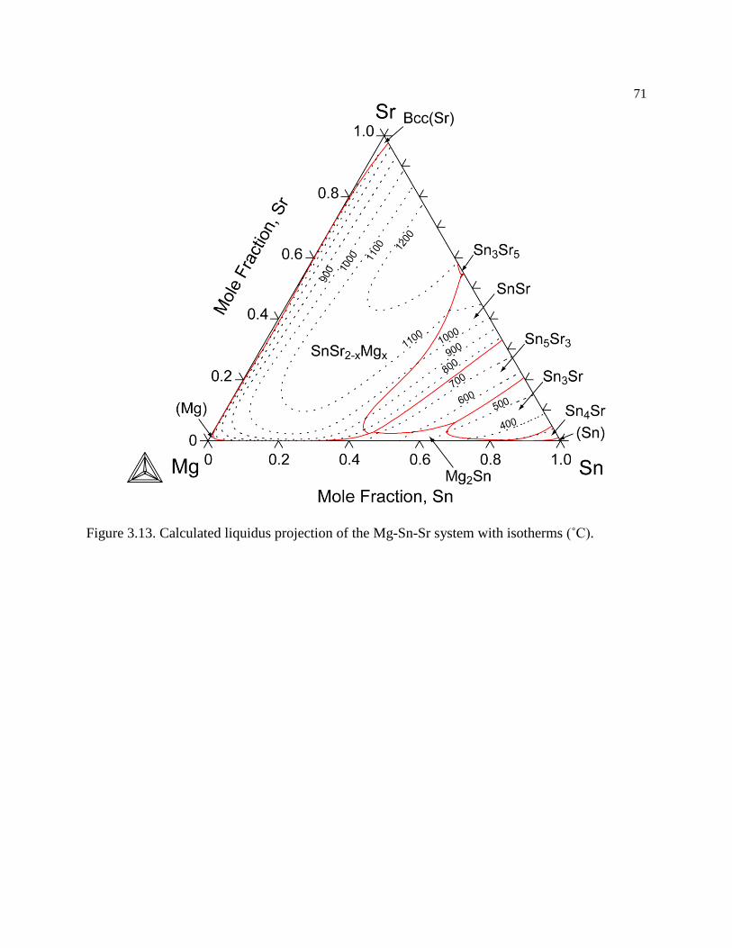
71
Figure 3.13. Calculated liquidus projection of the Mg-Sn-Sr system with isotherms (˚C).
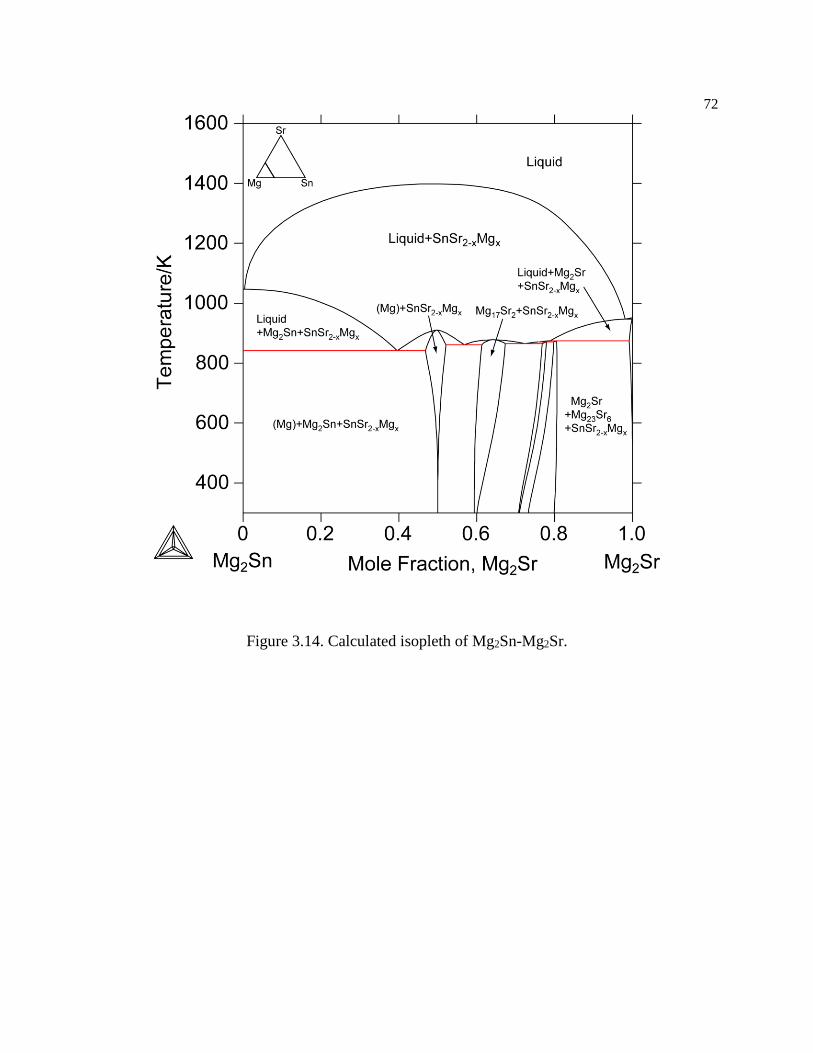
72
Figure 3.14. Calculated isopleth of Mg2Sn-Mg2Sr.
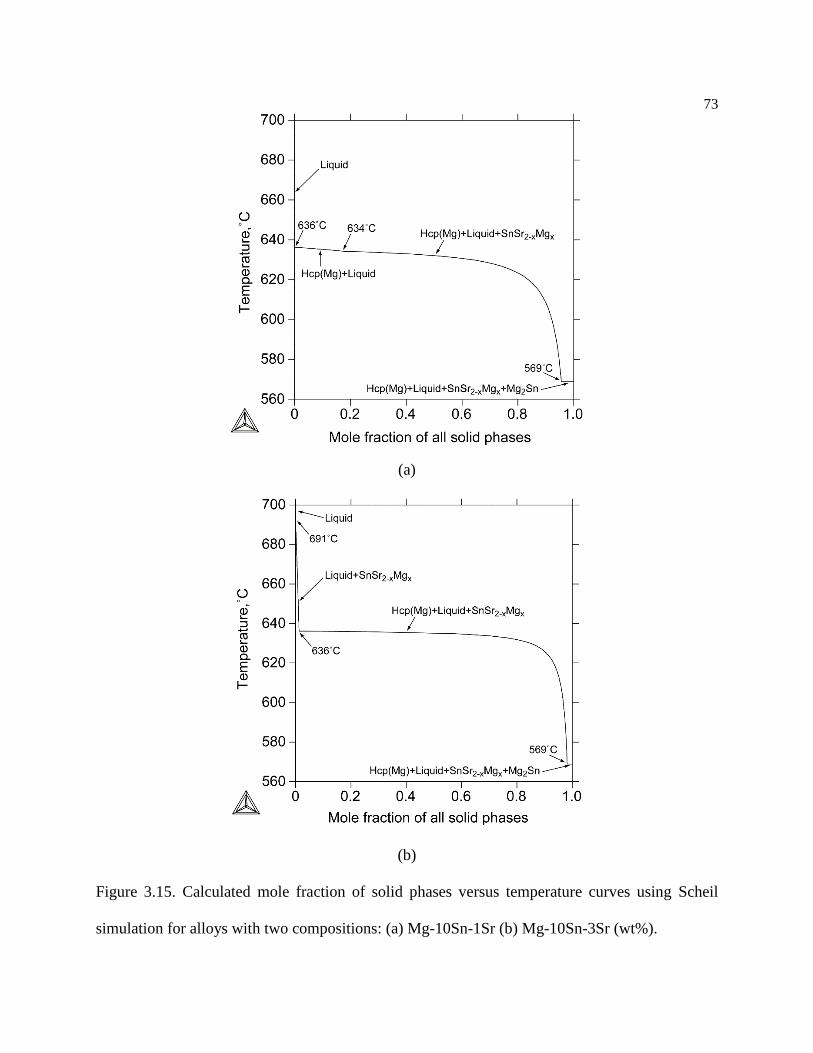
73
(a)
(b)
Figure 3.15. Calculated mole fraction of solid phases versus temperature curves using Scheil
simulation for alloys with two compositions: (a) Mg-10Sn-1Sr (b) Mg-10Sn-3Sr (wt%).
74
Chapter 4
First-principles calculations and thermodynamic modeling of Ce-Sn system with
extension to Mg-Ce-Sn system
4.1 Introduction
In recent years, magnesium alloys have generated great interest due to their lightweight,
earth abundance, high specific strength, and good castablity [1]. These properties make Mg alloys
attractive for automotive, aerospace and other light-weight structural applications [3]. Commercial
Mg alloys for automotive applications are mostly Mg-Al based (AZ and AM series) systems,
which offer good room-temperature strength, corrosion resistance, and die castability. However,
these alloys suffer poor creep resistance at elevated temperatures (>125 C) due to the poor thermal
stability of the Mg17Al12 phase, which makes them inadequate for automotive powertrain
applications [60]. Mg-Sn based alloys have received renewed attention since 2006 due to their
potential applications at elevated temperatures [62–66]. The Mg-Sn system is an age-hardenable
system and exhibits good castability due to the eutectic nature of its phase diagram [65]. The main
precipitate phase Mg2Sn in Mg-Sn based alloys has a melting point of 770 ˚C, which is much
higher than that of Mg17Al12 phase (462 ˚C) in Mg-Al alloys [67]. These properties make Mg-Sn
based alloys a promising Mg alloy system for automobile powertrain applications at elevated
temperatures. Further rational design of Mg-Sn based alloys requires accurate knowledge of the
thermodynamics of Mg-Sn-X (single additions) and Mg-Sn-(X-Y) (double additions) systems,
which is largely unavailable in the literature [63]. The CALPHAD (CALculation of PHAse

75
Diagrams) method [11] has proven to be an invaluable method to model and predict phase
equilibria in multi-component materials. Therefore, there is a pressing need to develop
thermodynamic databases of Mg-Sn based alloys based on the CALPHAD technique [69].
Several Sn-containing binary systems, such as Sn-Ca [73], Sn-Ce [74], Sn-Na [75] and Sn-
Sr [76] systems, exhibit short-range ordering in the liquid phase. Consequently, there are steep
liquidus and many stable intermetallic compounds with much higher melting point than their
constituent elements in these binary phase diagrams. Traditional modeling strategy of these
compounds using the Neumann-Kopp approximation yields artificial kinks in the heat capacity
descriptions at the melting point of the constituent elements. First-principles quasi-harmonic
Debye model [35] are used in the present work to directly predict the finite-temperature
thermodynamic properties of the intermetallic compounds in the Ce-Sn and Mg-Ce-Sn systems,
which provide data for robust CALPHAD modeling and resolve the heat capacity artifact problem
due to the Neumann-Kopp approximation. The Ce-Sn binary system is re-modeled in the present
work as an improvement of Dong et al.’s previous modeling work [107]. Thermodynamic
descriptions of the Mg-Sn [78] and Mg-Ce [108] systems are taken from the literature. Combining
the thermodynamic models of three constituent binary systems, the thermodynamic description of
the Mg-Ce-Sn ternary system is obtained, and phase relations in the ternary system are predicted.
4.2 Literature Review
The literature review of Mg-Sn system is described in Section 3.2. The thermodynamic
description of Mg-Ce system is taken from Hui et al’s work [108]. A detailed literature review of
Mg-Ce system can be found in their paper [108].
76
The review of thermochemical data of the Ce-Sn system can be found in [109] and will not
be repeated here. A literature review of the phase equilibrium data will be given. The first Ce-Sn
phase diagram was obtained by Vogel [110] using thermal and metallographic analyses. This
diagram is considered as the first while incorrect rare earth binary phase diagram. He continued to
investigate this system by focusing on the 75–100 at% Sn rich part [111]. However, the works by
Vogel suffer some accuracy issues. In 1988, a new partial phase diagram of this system was
determined by differential thermal analysis (DTA) [112], which covered the part from 0–50 at%
Sn. Riani et al. [109] summarized all the available information of the Ce-Sn system including the
phase equilibrium information, crystal structures of the intermetallic compounds, and
thermochemical data. Several new compounds were identified in the Ce-Sn system. Since the
solubility range of Ce11Sn10 was not confirmed by other experiments, it wasn’t adopted in the
current modeling. The phase boundary data by Franceschi [112] was mainly used in the current
modeling.
Unfortunately there is no experimental information available for the Mg-Ce-Sn system.
The Mg-Ce-Sn ternary description is purely extrapolated from the thermodynamic descriptions of
the constituent binaries.
4.3 Calculation and modeling details
4.3.1 First-principles calculations
First-principles calculations based on the density functional theory were employed to
predict the finite-temperature thermodynamic properties of phases of interest. The Vienna ab initio
simulation package (VASP) 5.2.12 [49] was used to perform the first-principles calculations within

77
the generalized gradient approximation (GGA) of Perdew, Burke, and Ernzerhof (PBE) [46]. The
electronic states 3s2, 5s25p2, and 6s25d14f1 were considered as valence states for Mg, Sn, and Ce,
respectively. The ion-electron interactions were described by the projector augmented wave
method (PAW) [97] with an energy cutoff of 350 eV for all the structures. The cell volume, shape
and atomic arrangements were fully relaxed using the Methfessel-Paxton method and at least 5000
k-points per reciprocal atom based on the Monkhorst-Pack scheme for the Brillouin-zone sampling
was used. For hcp Mg, the Gamma centered scheme was used for the Brillouin-zone sampling.
Among the six intermetallic compounds in the Ce-Sn system, the Ce5Sn4 compound also
has very high melting point. Therefore, their thermodynamic properties are of great importance in
the present thermodynamic modeling. Due to the scarcity and likely inaccuracies of the
thermochemical data in this system, it is thus necessary to attempt to describe the finite temperature
thermodynamic properties of these compounds through first-principles. In the case of perfectly
ordered, defect-free non-magnetic crystalline metallic phases, the major contributions to the free
energy come from the vibrational (phonon) and thermal electronic excitations [98].
Using the quasi-harmonic approach [98], the Helmholtz free energy of a stoichiometric
phase as a function of volume V and temperature T, 𝐹(𝑉, 𝑇), is given by [98]
𝐹(𝑉, 𝑇) = 𝐸0(𝑉) + 𝐹𝑣𝑖𝑏(𝑉, 𝑇) + 𝐹𝑒𝑙𝑒(𝑉, 𝑇) (4.1)
where 𝐸0(𝑉) is the 0 K total energy, 𝐹𝑣𝑖𝑏(𝑉, 𝑇) the vibrational free energy of the lattice ions, and
𝐹𝑒𝑙𝑒(𝑉, 𝑇) the thermal electronic contribution to the free energy. At zero pressure, the Helmholtz
energy of the system equals to the Gibbs energy. In the present work, 𝐸0(𝑉) is obtained via first-
principles calculations for each phase in the system. With the Debye-Gruneisen model validated
by phonon calculations, 𝐹𝑣𝑖𝑏(𝑉, 𝑇) for other compounds are obtained only from the Debye-
Gruneisen model for the sake of simplicity and efficiency. Since the elements of interest in the
78
present work are metallic, the thermal electronic contribution to the Helmholtz energy is included
due to electronic excitations at high temperatures around the Fermi level. The thermal electronic
contribution to Helmholtz energy is based on the electronic Density of States (DOS) using Fermi-
Dirac statistics [98].
For the compounds Ce3Sn, Ce5Sn3, Ce5Sn4, Ce11Sn10, Ce3Sn7, Ce2Sn5, and CeSn3, we use
quasi-harmonic Debye model. In the quasi-harmonic Debye model [35], the vibrational
contribution to Helmholtz energy is described as
𝐹𝑣𝑖𝑏(𝑉, 𝑇) =9
8𝑘𝐵Θ𝐷(𝑉) + 𝑘𝐵𝑇 [3 ln (1 − 𝑒−
ΘD(V)T ) − 𝐷 (
ΘD(𝑉)
T)] (4.2)
where Θ𝐷 is the Debye temperature, 9
8𝑘𝐵Θ𝐷(𝑉) the zero-point energy at 0 K, and 𝑘𝐵 the
Boltzmann’s constant. All the other implementation procedures of quasi-harmonic Debye model
are the same as described in Section 3.3.1.
A four-parameter Birch-Murnaghan equation of state (EOS) [51] is adopted herein to fit
𝐸0(𝑉), represented as
𝐸(𝑉) = 𝑎 + 𝑏𝑉−2/3 + 𝑐𝑉−4/3 + 𝑑𝑉−2 (4.3)
Additionally, our experiences show that for metallic systems, the EOS used in the present
work has a lower fitting error [35]. The EOS thus obtained is used to calculate the parameters
needed in the Debye model.
For an ordered phase in the Mg-Ce-Sn system, the enthalpy of formation, Δ𝐻𝑓 , is
determined from:
79
∆𝐻𝑓
𝑀𝑔𝑥𝐶𝑒𝑦𝑆𝑛𝑧 = 𝐻(𝑀𝑔𝑥𝐶𝑒𝑦𝑆𝑛𝑧) −𝑥
𝑥+𝑦+𝑧𝐻(𝑀𝑔) −
𝑦
𝑥+𝑦+𝑧𝐻(𝐶𝑒) −
𝑧
𝑥+𝑦+𝑧𝐻(𝑆𝑛) (4.4)
where H’s are enthalpies from the finite temperature first-principles Debye or phonon calculations,
and the reference states for compounds are set as hcp (hexagonal closed packed) for Mg, fcc (face-
centered cubic) for Ce, and bct (body-centered tetragonal) for Sn, respectively, namely, the stable
structures of these pure elements at the temperature of 298.15 K and the pressure of 1 bar.
4.3.2 CALPHAD modeling
The Gibbs energy functions of pure Mg, Sn and Ce are taken from the SGTE (Scientific
Group Thermodata Europe) pure element database [37] as is implemented in the PURE4 database
in Thermo-Calc [36]. The intermetallic compounds, Ce3Sn, Ce5Sn3, Ce5Sn4, Ce11Sn10, Ce3Sn7,
Ce2Sn5, and CeSn3, are modeled in the present work. The liquid phase is modeled using an
associate solution model to account for its short-range order behavior.
Thermodynamic models
In the present work, the Ce3Sn, Ce5Sn3, Ce5Sn4, Ce11Sn10, Ce3Sn7, Ce2Sn5, and CeSn3
phases are treated as stoichiometric compounds. The Gibbs energy of the intermetallic compound
phases are described as:
𝐺𝑀𝑔𝑥𝑆𝑛𝑦𝐶𝑒𝑧 − 𝐻𝑆𝐸𝑅 = 𝑎 + 𝑏𝑇 + 𝑐𝑇𝑙𝑛(𝑇) + 𝑑𝑇2 + 𝑒𝑇−1 + 𝑓𝑇3 (4.5)
where a, b, c, d, e and f are model parameters determined from free energy calculated from the
finite-temperature first-principles methods described above. 𝐻𝑆𝐸𝑅 is the stable element reference
(SER) state that refers to the enthalpies of hcp-Mg, fcc-Ce and bct-Sn at 298.15 K and 1 bar.
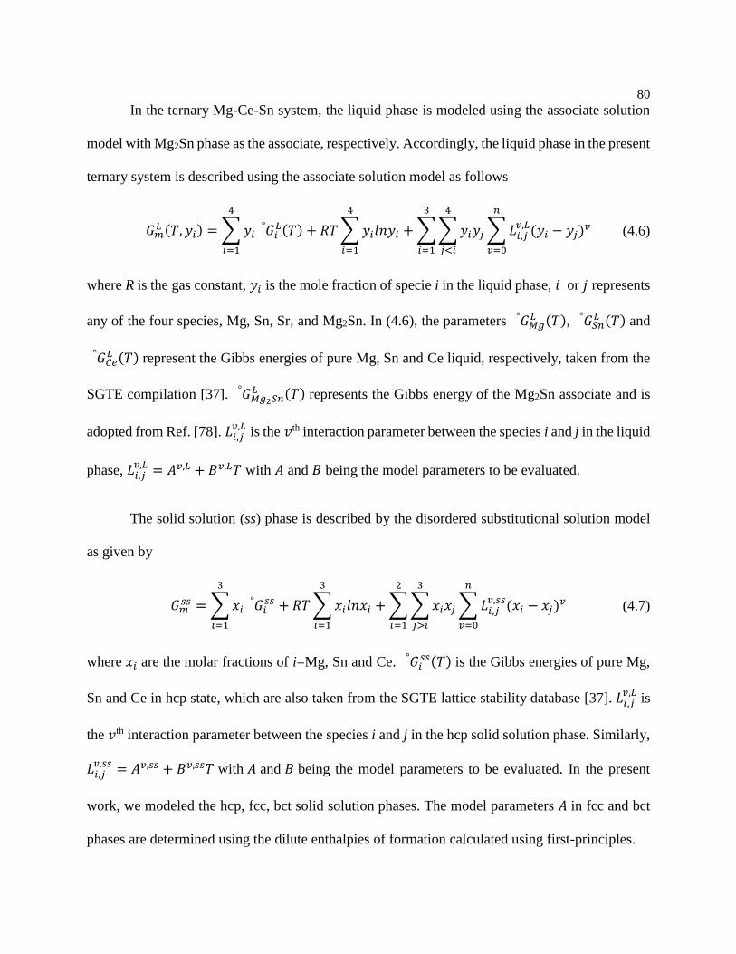
80
In the ternary Mg-Ce-Sn system, the liquid phase is modeled using the associate solution
model with Mg2Sn phase as the associate, respectively. Accordingly, the liquid phase in the present
ternary system is described using the associate solution model as follows
𝐺𝑚𝐿 (𝑇, 𝑦𝑖) = ∑ 𝑦𝑖 𝐺°
𝑖𝐿(𝑇)
4
𝑖=1
+ 𝑅𝑇 ∑ 𝑦𝑖𝑙𝑛𝑦𝑖
4
𝑖=1
+ ∑ ∑ 𝑦𝑖𝑦𝑗 ∑ 𝐿𝑖,𝑗𝑣,𝐿(𝑦𝑖 − 𝑦𝑗)𝑣
𝑛
𝑣=0
4
𝑗<𝑖
3
𝑖=1
(4.6)
where R is the gas constant, 𝑦𝑖 is the mole fraction of specie i in the liquid phase, 𝑖 or 𝑗 represents
any of the four species, Mg, Sn, Sr, and Mg2Sn. In (4.6), the parameters 𝐺°𝑀𝑔𝐿 (𝑇), 𝐺°
𝑆𝑛𝐿 (𝑇) and
𝐺°𝐶𝑒𝐿 (𝑇) represent the Gibbs energies of pure Mg, Sn and Ce liquid, respectively, taken from the
SGTE compilation [37]. 𝐺°𝑀𝑔2𝑆𝑛𝐿 (𝑇) represents the Gibbs energy of the Mg2Sn associate and is
adopted from Ref. [78]. 𝐿𝑖,𝑗𝑣,𝐿
is the 𝑣th interaction parameter between the species i and j in the liquid
phase, 𝐿𝑖,𝑗𝑣,𝐿 = 𝐴𝑣,𝐿 + 𝐵𝑣,𝐿𝑇 with 𝐴 and 𝐵 being the model parameters to be evaluated.
The solid solution (ss) phase is described by the disordered substitutional solution model
as given by
𝐺𝑚𝑠𝑠 = ∑ 𝑥𝑖 𝐺°
𝑖𝑠𝑠
3
𝑖=1
+ 𝑅𝑇 ∑ 𝑥𝑖𝑙𝑛𝑥𝑖
3
𝑖=1
+ ∑ ∑ 𝑥𝑖𝑥𝑗 ∑ 𝐿𝑖,𝑗𝑣,𝑠𝑠(𝑥𝑖 − 𝑥𝑗)𝑣
𝑛
𝑣=0
3
𝑗>𝑖
2
𝑖=1
(4.7)
where 𝑥𝑖 are the molar fractions of i=Mg, Sn and Ce. 𝐺°𝑖𝑠𝑠(𝑇) is the Gibbs energies of pure Mg,
Sn and Ce in hcp state, which are also taken from the SGTE lattice stability database [37]. 𝐿𝑖,𝑗𝑣,𝐿
is
the 𝑣th interaction parameter between the species i and j in the hcp solid solution phase. Similarly,
𝐿𝑖,𝑗𝑣,𝑠𝑠 = 𝐴𝑣,𝑠𝑠 + 𝐵𝑣,𝑠𝑠𝑇 with 𝐴 and 𝐵 being the model parameters to be evaluated. In the present
work, we modeled the hcp, fcc, bct solid solution phases. The model parameters 𝐴 in fcc and bct
phases are determined using the dilute enthalpies of formation calculated using first-principles.
81
The modeling procedures of Mg-Ce-Sn system are similar to those in Mg-Sn-Sr system as
described in Section 3.3.2.
4.4 Results and Discussion
Figure 4.3 shows the modeled Ce-Sn binary phase diagram based on the current
thermodynamic parameters. The experimental enthalpies of formation by [113] were used in the
present modeling along with the entropies of formation calculated from the quasi-harmonic Debye
model in the present work. The enthalpy of formation of Ce2Sn5 is slightly above the convex hull
in the Ce-Sn system, as shown in Figure 4.4. Therefore, the Ce2Sn5 compound decomposes at about
450 K according to the current modeling.
First-principles quasi-harmonic Debye model was used to predict the heat capacities as
well as entropies of the binary compounds in the Ce-Sn system. Figure 4.6 shows the calculated
heat capacities and entropies from first-principles based Debye model for compound CeSn3 and
Ce3Sn5. As is shown in Figure 4.6, the use of finite-temperature first-principles data is better than
the Neuman-Kopp approximation in terms of describing the heat capacities of compounds. The
constituent pure elements Ce and Sn both have relatively low melting points compared with the
binary Ce-Sn intermetallic compounds. For the intermetallic compound whose melting point is
higher than its constituent pure elements, finite-temperature first-principles calculation can offer a
more physical description of the thermodynamic properties of these compounds, avoiding the
artificial kinks as shown in Figure 4.6.
Figure 4.7 shows the isothermal sections of the isothermal section and the Mg-rich corner
of the Mg-Ce-Sn system at 793K. Specific phase regions can be identified to have stable high
82
temperature stable phase as the strengthening precipitate for high temperature Mg alloys, such as
Mg2Sn. The compound Ce5Sn4 which has the highest melting point is very stable at low
temperature. It is very easy to precipitate out in the Mg-Ce-Sn system. This is also demonstrated
by the Scheil simulation in Figure 4.9.
4.5 Conclusions
All the experimental phase diagrams and thermodynamic data of the Ce-Sn and Mg-Ce-Sn
systems available in the literature have been critically reviewed. The finite-temperature
thermodynamic properties for seven stoichiometric compounds in the Mg-Ce-Sn system are
computed by phonon and Debye model with inputs from the first-principles calculations. It
provides robust input thermochemical data for modeling and avoids the artifact of heat capacity
description from the the Neumann-Kopp approximation. The short range behavior in the liquid
phase of the Mg-Ce-Sn system is well described by the associate solution model. A complete set
of self-consistent thermodynamic parameters is obtained based on the literature data and the first-
principles calculation results.
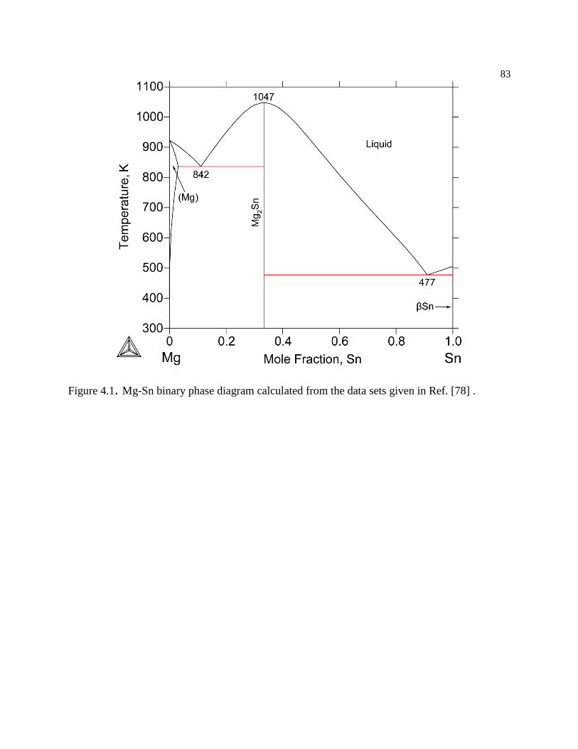
83
Figure 4.1. Mg-Sn binary phase diagram calculated from the data sets given in Ref. [78] .
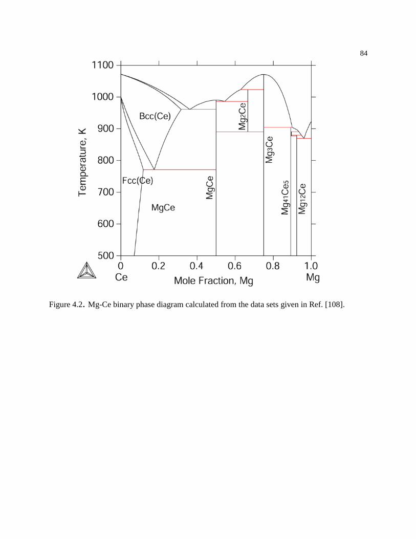
84
Figure 4.2. Mg-Ce binary phase diagram calculated from the data sets given in Ref. [108].
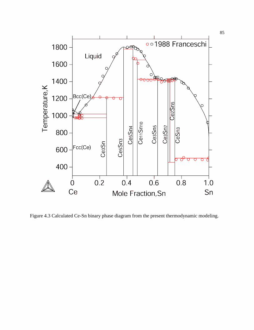
85
Figure 4.3 Calculated Ce-Sn binary phase diagram from the present thermodynamic modeling.
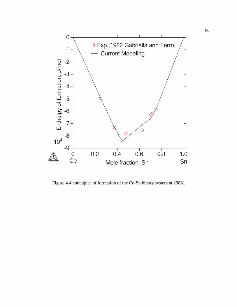
86
Figure 4.4 enthalpies of formation of the Ce-Sn binary system at 298K.

87
Figure 4.5 Enthalpy of mixing in the liquid phase of Ce-Sn binary system at 1870K.
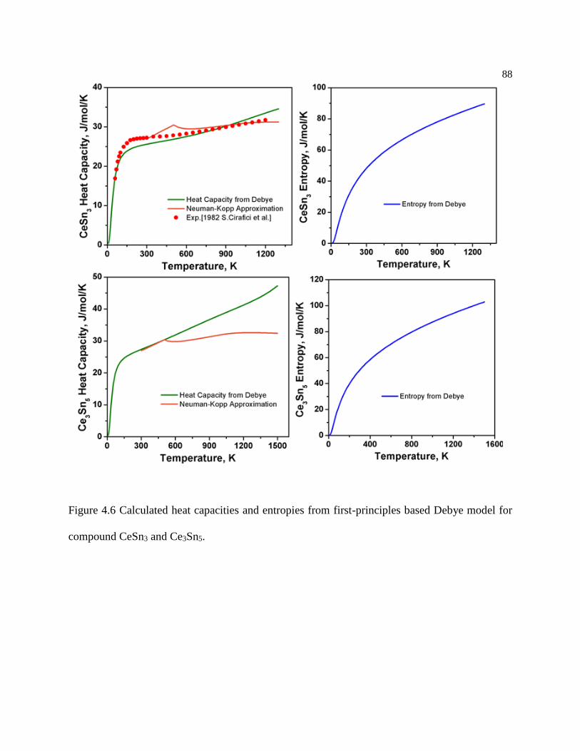
88
Figure 4.6 Calculated heat capacities and entropies from first-principles based Debye model for
compound CeSn3 and Ce3Sn5.

89
Figure 4.7 Isothermal section and the Mg-rich corner of the Mg-Ce-Sn system at 793K
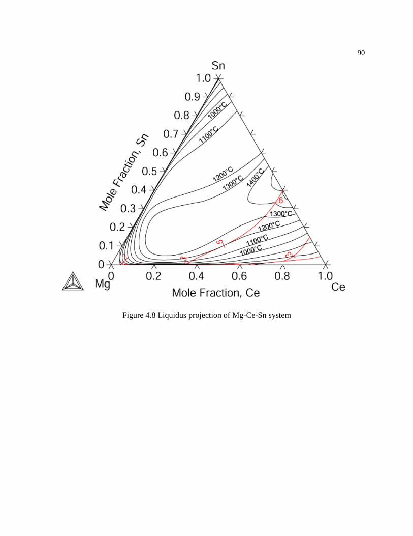
90
Figure 4.8 Liquidus projection of Mg-Ce-Sn system

91
Figure 4.9 Scheil simulation of Mg-Ce-Sn alloys.
92
Chapter 5
First-principles calculations of the self-diffusion coefficients in hcp Mg
5.1 Introduction
In recent years, magnesium (Mg) alloys have received an increasing interest due to their
low density, earth abundance, high specific strength, and good castability [1]. These properties
make Mg alloys attractive for automotive, aerospace, and other light-weight structural applications
[3]. The majority of Mg alloys derives their mechanical properties from precipitation hardening
[9], while the study of precipitation process demands accurate thermodynamic and kinetic
(diffusion) data. Thermodynamics of Mg alloys has been extensively studied, and several
comprehensive thermodynamic databases have been established [4]. However, the kinetics of Mg
alloys has been studied to a far lesser extent, especially diffusion coefficients of various solutes in
Mg. Due to the issues related to corrosion, oxidation, and contamination during sample preparation
in diffusion measurements, few experimental data are available in the literature for diffusion
coefficients of solutes in Mg [5].
Self-diffusion coefficients in Mg is important as it forms a baseline of diffusion rate in hcp
Mg. There have been numerous experimental investigations in the literature about self-diffusion
in Mg [114–117]. Ganeshan et al. also [33] used first-principles calculations to study the self-
diffusion coefficients of Mg. However, their DFT calculation suffer from inaccuracies due to the
choice of exchange-correlation (X-C) functionals. A more systematic investigation of self-
diffusion in Mg using different X-C functionals is needed.

93
5.2 Diffusion theory in hcp
For the hcp lattice, the crystal anisotropy results in two unique solute jumps, one within
the basal plane and the other between adjacent basal planes. These two solute jumps in the hcp
structure are illustrated in Figure 5.1. This leads to two distinctive diffusion tensors. The diffusion
coefficient perpendicular to the c-axis, D , results from jumps between the adjacent basal planes
and jumps within the basal plane; while the diffusion coefficient parallel to the c-axis, D ,
attributes to jumps between the adjacent basal planes only. Correspondingly, the diffusion
coefficients can be calculated using the following equations [118]:
213
2v Bx X Ab XD C a f f
(5.1)
23
4v Az XD C c f (5.2)
where a and c are lattice parameters of hcp lattice, Cv corresponds to vacancy concentration
adjacent to the solute atom, X and X are the solute-vacancy exchange jump frequencies
within and out of the basal plane, respectively, Bxf is the partial correlation factor for the solute
jump within a basal plane, Abf is the partial correlation factor corresponding to the horizontal
component of a solute jump into an adjacent basal plane, and Azf is the partial correlation factor
corresponding to the vertical component of a solute jump into the adjacent basal plane. Details of
the calculations of these variables are given below.
94
5.2.1 Vacancy concentration
The vacancy concentration in pure hcp Mg, Cv in Eqs. (5.1) and (5.2) in the dilute limit, is
calculated by a Boltzmann relation:
0
expf
v
B
GC
k T
(5.3)
where 0
fG is the vacancy formation free energy in pure Mg without solute, as is calculated by
0
1 1
1Mg Va Mgf N N
NG G G
N
(5.4)
where Va indicates a vacancy, and N the number of lattice sites in the supercell.
5.2.2 Jump frequencies of solutes
Once a vacancy adjacent to a solute atom is formed, the solute atom has to overcome the
migration barrier to exchange with the vacancy. Based on Eyring’s reaction rate theory [56] of
activated complex, as applied by Wert and Zener [119] to solute diffusion in solids, the solute-
vacancy exchange jump frequencies within and between the basal planes X and X in their
general form can be written as:
exp mB
B
Gk T
h k T
(5.5)
where m TS ISG G G is the solute migration free energy barrier with TSG being the free energy
of the transition state (TS) and ISG the free energy of the initial state (IS). A detailed discussion
of Eq. (5.5) at the high temperature and low temperature ranges is given by Wimmer et al. [120].
95
Instead of using Vineyard’s harmonic TST [27,121] which requires computation of full phonon
frequencies, we calculate the jump frequency directly from free energy calculations using quasi-
harmonic Debye model as discussed in Section 5.3 Computational details.
5.3 Computational details
First-principles calculations based on DFT were employed to calculate the free energies
needed in the diffusion equations and the 8-frequency model. The ion-electron interaction was
described by the projector augmented plane-wave (PAW) method [48] and the X-C functional was
described by an improved GGA of PBEsol [32], as implemented in the VASP 5.3.2 code [97]. The
suitability of PBEsol for the present study is discussed in the Section 5.4.2. An energy cut-off of
350 eV was used for the plane-wave expansion of the electronic wave functions.
5.3.1 Supercell size and k-point density
Tests were performed on pure Mg to estimate the convergence of the calculation results
with respect to the supercell size and k-point density. On the basis of these tests, the vacancy
formation energy and migration energies are estimated to be converged to within a precision of
approximately 0.01 eV.
After tests of supercell size, we chose a 64-atom supercell (4×4×2 conventional hcp unit
cells) for most solutes, which was sufficient to isolate the vacancy and solute atom from the
periodic images. All structural degrees of freedom (ionic coordinates, cell volume, and cell shape)
in the supercell were fully relaxed via a conjugate gradient method to an energy convergence of
10-5 eV/atom, followed by a final static calculation using the tetrahedron method with Blöchl

96
corrections [122] with energy convergence of 10-6 eV/atom to get the accurate total energy.
Although constant volume and cell shape were used in other diffusion calculations [27,123,124],
full relaxation of all degrees of freedom can result in more accurate local strain and generate the
useful quantity XV , which will be discussed in Section 6.4.1 Solute-vacancy binding energy. An
8×8×9 -centered k-point mesh was used for the 64-atom supercell for the electronic integration
in the Brillouin zone.
5.3.2 Transition state search
To determine the position of the saddle point and associated minimum-energy pathway
during solute migration, calculations were performed employing the CI-NEB method [25] with 3
images. The two end-point structures, i.e. the initial and final structures, were fully relaxed first.
The same supercell size and k-point settings were used in the CI-NEB calculations as are
mentioned in the above discussion. Such calculations were performed for all the solute (solvent)-
vacancy exchange in the 8-frequency model for each investigated elements. Unlike hcp Ti (as well
as hcp Zr) with two saddle points [125], in all cases the energy was found to display a single
maximum, corresponding to the saddle point at the high-symmetry position located half way
between neighboring sites.

97
5.3.3 The quasi-harmonic approach
Vibrational contributions to the free energies were calculated using the quasi-harmonic
approximations from phonon or Debye model. Helmholtz free energy of a configuration as a
function volume (V) and temperature (T) can be expressed as [35]:
0( , ) ( ) ( , ) ( , )vib elF V T E V F V T F V T (5.6)
where 0 ( )E V is the static energy at 0 K without the zero-point vibrational energy, ( , )vibF V T the
vibrational contribution, and ( , )elF V T the thermal-electronic contribution. Note that at zero
pressure, the Helmholtz free energy is equal to the Gibbs free energy. In the present work, 0 ( )E V
was calculated via first-principles directly, and ( , )elF V T obtained by integrating the electronic
density of states [98]. It is found that ( , )elF V T has a negligible contribution to the total free energy
compared with ( , )vibF V T , but it was still considered in the present work for the sake of
completeness. Based on the previous work [31] from our group, the quasi-harmonic Debye model
is sufficient to describe well the vibrational contribution to free energy in diffusion calculations
compared with phonon calculations and can save tremendous computing resources. Therefore,
( , )vibF V T for all the initial and transition states were calculated using the quasi-harmonic Debye
model in the present work. We still calculated the self-diffusion coefficients in Mg using quasi-
harmonic phonon model for comparison with the quasi-harmonic Debye model, as shown in Figure
5.4.
In the quasi-harmonic phonon model, the vibrational contribution to Helmholtz energy is
obtained by the integration of calculated phonon density of states. The details of implementation
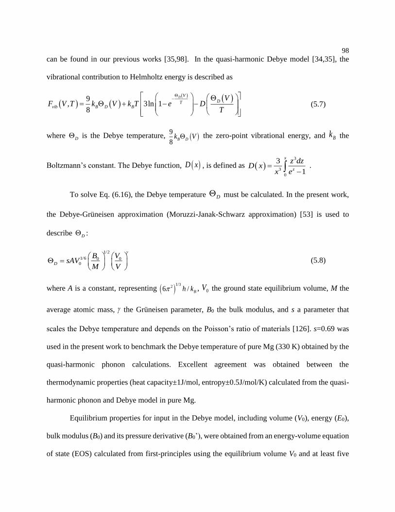
98
can be found in our previous works [35,98]. In the quasi-harmonic Debye model [34,35], the
vibrational contribution to Helmholtz energy is described as
9
, 3ln 18
D V
DTvib B D B
VF V T k V k T e D
T
(5.7)
where D is the Debye temperature, 9
8B Dk V the zero-point vibrational energy, and Bk the
Boltzmann’s constant. The Debye function, D x , is defined as 3
3
0
3
1
x
z
z dzD x
x e
.
To solve Eq. (6.16), the Debye temperature D must be calculated. In the present work,
the Debye-Grüneisen approximation (Moruzzi-Janak-Schwarz approximation) [53] is used to
describe D :
1/2
1/6 0 00D
B VsAV
M V
(5.8)
where A is a constant, representing 1/3
26 / Bh k , 0V the ground state equilibrium volume, M the
average atomic mass, the Grüneisen parameter, B0 the bulk modulus, and s a parameter that
scales the Debye temperature and depends on the Poisson’s ratio of materials [126]. s=0.69 was
used in the present work to benchmark the Debye temperature of pure Mg (330 K) obtained by the
quasi-harmonic phonon calculations. Excellent agreement was obtained between the
thermodynamic properties (heat capacity±1J/mol, entropy±0.5J/mol/K) calculated from the quasi-
harmonic phonon and Debye model in pure Mg.
Equilibrium properties for input in the Debye model, including volume (V0), energy (E0),
bulk modulus (B0) and its pressure derivative (B0’), were obtained from an energy-volume equation
of state (EOS) calculated from first-principles using the equilibrium volume V0 and at least five

99
additional volumes (0.96, 0.98, 1.02, 1.04, and 1.06 with respect to V0). A four parameter Birch-
Murnaghan EOS was used herein to fit the energy-volume data. It is represented in its linear form
[35]
2/3 4/3 2( )E V a bV cV dV (5.9)
where a, b, c, and d are fitting parameters. This EOS was adopted because it has been previously
shown to be able to produce accurate properties for many materials systems [35,127]. It should be
noted that the EOS for the saddle point configuration was obtained without relaxing each
additional volume in order to maintain its saddle point structure. It is observed that the value of B0’
is quite sensitive to the EOS fitting and is always around 4 in all the EOS fittings. When the fitted
energy-volume curve was not smooth enough due to the scattered energy-volume points which
indicates the B0’ value is far away from 4, the value from a pressure-volume fitting [128] was used
instead.
5.4 Results and Discussion
5.4.1 Thermodynamic properties of pure hcp Mg
In order to validate the applicability of quasi-harmonic Debye model, thermodynamic
properties (heat capacity Cp and entropy S) were predicted using both quasi-harmonic Debye and
phonon model and were compared with experimental data, as shown in 2. Excellent agreement
were achieved between computation and experiments.

100
5.4.2 Vacancy formation energy in pure Mg
Vacancy formation energy 0
fE is critical for obtaining accurate diffusion coefficients
because it is exponentially related to the vacancy concentration in pure Mg, which is a term
presented in all the vacancy-mediated diffusion equations in the present work. Previously
measured [129–135] and calculated [22,33,136–138] values for 0
fE in Mg are listed in Table 5.1
along with our present calculations and are in good agreement. Beevers [129], Mairy et al. [130],
and Tzanétakis et al. [132,135] measured 0
fE in Mg using electrical resistivity method, with their
measured values ranging from 0.79 eV to 0.89 eV. Janot et al. [131] measured 0
fE in Mg using
the differential dilatometry and obtained 0.58 eV. The work of Janot et al. [131] was subsequently
criticized by Tzanétakis et al. [132] and Hood [139] for suffering large uncertain errors in the
thermal dilatometry measurements. Segers et al. [133] and Hautojärvi et al. [134] performed
positron annihilation spectroscopy measurements of 0
fE in Mg and obtained consistent values of
around 0.85 eV. The vacancy formation entropy was also estimated to be 2 kB in the work of
Hautojärvi et al. [134]. Our DFT calculated vacancy formation enthalpy and entropy from PBEsol
compare especially well with the more reliable positron annihilation spectroscopy data [133,134].
The introduction of vacancy into a system creates a small amount of internal surface inside
the supercell. It has been indicated in several studies [140,141] on vacancy formation in metallic
systems that LDA will describe the internal surface around a vacancy better than GGA due to an
error cancellation effect: LDA largely overestimates the exchange energy of a free metal surface,
but underestimates by approximately the same magnitude the correlation energy. This results in a
reasonable net total value of the surface energy [142]. In the present work, we applied the X-C
functional of PBEsol because it includes the surface correction based on a gradient expansion of

101
the exchange energy and a final fit of the X-C energy to that of surface jellium [32]. Therefore it
is able to describe well the internal surface of the vacancy. Consequently, the vacancy formation
energy values calculated from LDA and PBEsol agree very well with those measured by the
positron annihilation spectroscopy in the literature, which is around 0.85 eV for Mg [139]. GGA
systematically underestimates the vacancy formation energy by around 0.1 eV, as is shown by two
of our previous studies [33,136] listed in Table 5.1.
We also tested the effect of supercell size on the calculated vacancy formation energy and
found that 64-atom supercell is sufficient to converge the result. Using the vacancy formation
energy and entropy in pure hcp Mg calculated from PBEsol (0.86 eV and 2.1 kB, respectively) the
equilibrium vacancy concentration at 920 K near the melting point of Mg is calculated to be a
reasonable value of 1.5×10⁻⁴ according to Eq. (5.3). The thermodynamic properties of vacancy
formation in hcp Mg are shown in Figure 5.3. Recently, Glensk et al. [143] have demonstrated that
the traditional linear Arrhenius assumption to extrapolate the experimental T=0 K enthalpy of
vacancy formation is not accurate using Al and Cu as examples. They proposed that linear
Arrhenius assumption needs to be replaced by a local Grüneisen theory with a formation entropy
linear in the temperature by considering the anharmonic contribution to the vibrational free energy.
However, their proposed theory needs to be further validated in more materials systems.
5.4.2 Effects of X-C functionals
Figure 5.4 shows the calculated Mg self-diffusion coefficients using different X-C
functionals of LDA, GGA, and PBEsol compared with available experiments [114–117]. The self-
diffusion coefficients from PBEsol calculated by Debye model show the best agreement with
102
available experimental values. According to the Arrhenius diffusion equation, the slope of the
diffusion coefficient line in Figure 5.4 corresponds to the activation energy Q and the intersect
with vertical axis corresponds to the diffusion pre-factor D0. The enthalpies of vacancy formation
and migration mainly contribute to Q while the entropies of vacancy formation and migration
mainly contribute to D0.
Diffusion coefficients calculated using LDA yield a decent slope but a lower intersect,
while the calculations using GGA give a good intersect but a lower slope compared with
experiments. The reason is because LDA and GGA have different advantages in terms of getting
accurate properties. LDA is most suitable for vacancy formation energy due to its surface error
cancellation [144] as discussed in Section 5.4.1. But LDA causes significant overbinding in
metallic systems, evidenced by the underestimated Mg equilibrium lattice parameters (a0=3.112
[137], 3.12 [138], 3.141 [22], 3.133 Å [33] and c0=5.041 [137], 5.06 [138], 5.065 [22], 5.079 Å
[33]) compared with experiment (a0=3.209 Å and c0=5.211 Å [145]) in Table 5.1, which results in
a lower D0. On the contrary, although improper for vacancy formation energy, GGA is most
suitable to obtain the equilibrium and vibrational properties for metallic systems [50]. This
explains why the self-diffusion coefficients from LDA have a decent slope, i.e. the enthalpy-
related Q value, and a good intersect from GGA, i.e. the entropy-related D0 value. Since PBEsol
is a revised GGA that improves equilibrium properties of densely packed solids and their surfaces
[32], and possesses both advantages from LDA and GGA, it hence improves the predictions for
both Q and D0.
103
5.4.3 Comparison between Debye and phonon model
As shown in Figure 5.4, the calculated self-diffusion coefficients by the quasi-harmonic
Debye model shows better agreement with experiments than the quasi-harmonic phonon model.
The Debye and phonon models yield different entropies of vacancy formation and entropies of
vacancy migration, which attributes to the intersect difference (D0) between the self-diffusion
coefficients calculated by these two models. The Debye model has more accurate intersect
compared with experiments while the phonon model underestimates the D0 value by around half
an order of magnitude. Debye model is expected to perform well in systems where the differences
in vibrational free energy between structures can be explained by uniform shifts of the phonon
DOS, such as when the volume effect operates alone [54]. In the calculations of diffusion
coefficients in Mg, the major contribution to the entropic differences between different supercell
configurations is the solute size effect, as represented by the solute-induced volume change XV .
This is the reason for the success of Debye model. The present work shows that the Debye model
is a valid alternative for the calculations of diffusion coefficients that will reduce computational
time and complexity of the calculations. Similar conclusion has been drawn in a recent work on
the calculation of self-diffusion coefficients in fcc Ni [31].
5.5 Conclusion
In conclusion, we demonstrate that first-principles calculations based on density functional
theory can be used to predict the self-diffusion coefficient in hcp Mg successfully. PBEsol is able
to describe both the vacancy formation energy and the vibrational properties correctly. This gives
confidence in using this XC functional to predict the impurity diffusion coefficients in Mg.

104
Table 5.1 Comparison of experimental and first-principles calculated vacancy formation energies 0
fE and
equilibrium lattice parameters a0 and c0 in hcp Mg. First-principles results are calculated using different X-
C functionals of LDA, GGA, and PBEsol at 0 K and with various supercell sizes. Note that the
experimentally measured vacancy formation energies are usually assumed to be constant with respect to
temperature.
Method Supercell size (sites) a0 (Å) c0 (Å) Vacancy formation energy (eV) Reference
LDA 96 3.112 5.041 0.83 Chetty et al. [137]
LDA 54 3.12 5.06 0.83±0.07 Krimmel and Fahnle [138]
LDA 36 3.141 5.065 0.84 Mantina et al. [26]
LDA 36 3.133 5.079 0.81 Ganeshan et al. [33]
LDA 48,64,96,144 0.83±0.01 Shin and Wolverton [136]
GGA 36 3.195 5.176 0.72 Ganeshan et al. [25]
GGA 48,64,96,144 3.197 5.173 0.74±0.05 Shin and Wolverton [30]
PBEsol 36 3.172 5.152 0.83 This work
PBEsol 54 3.176 5.149 0.85 This work
PBEsol 64 3.175a 5.154a 0.86 This work
PBEsol 96 3.165 5.190 0.85 This work
Expt. ∆ρqb 0.89±0.06 Beevers [129]
Expt. ∆ρq 0.79±0.03 Tzanétakis et al. [132]
Expt. ∆ρq 0.83±0.03 Tzanétakis [135]
Expt. ∆ρeqc 0.81±0.02 Mairy et al. [130]
Expt. DDd 0.58±0.01 Janot et al. [131]
Expt. PASe 0.07
0.050.85
Segers et al. [133]
Expt. PAS 0.85 Hautojärvi et al. [134] a Experimental lattice parameters of Mg a0=3.209 Å and c0=5.211 Å at room temperature [145] b ∆ρq: electrical resistivity of quenched samples c ∆ρeq: electrical resistivity of thermal equilibrium samples d DD: differential dilatometry e PAS: positron annihilation spectroscopy
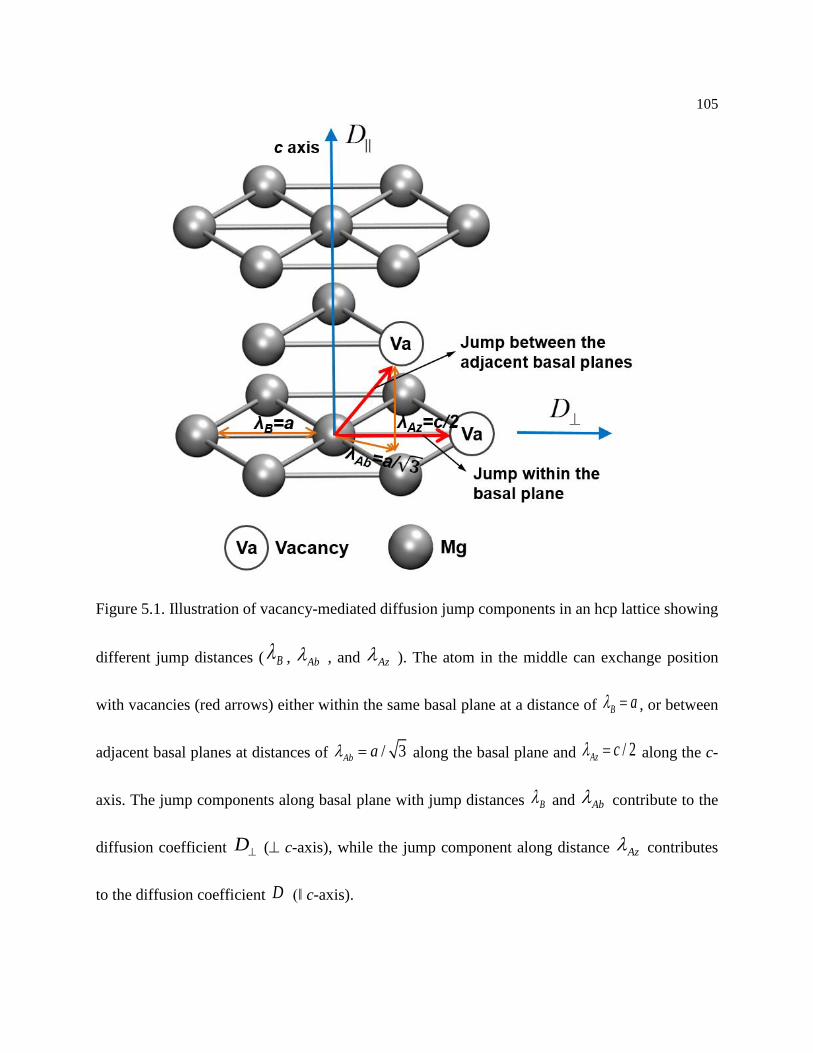
105
Figure 5.1. Illustration of vacancy-mediated diffusion jump components in an hcp lattice showing
different jump distances ( B , Ab , and Az ). The atom in the middle can exchange position
with vacancies (red arrows) either within the same basal plane at a distance of B a , or between
adjacent basal planes at distances of / 3Ab a along the basal plane and / 2Az c along the c-
axis. The jump components along basal plane with jump distances B and Ab contribute to the
diffusion coefficient D ( c-axis), while the jump component along distance Az contributes
to the diffusion coefficient D (‖ c-axis).

106
Figure 5.2 Predicted heat capacity Cp and entropy S of pure hcp Mg using Debye and phonon
model in comparison with SGTE experimental data.

107
Figure 5.3 Vacancy formation (a) enthalpy, (b) free energy, (c) entropy, and (d) vacancy
concentration as a function of temperature in pure hcp Mg calculated by the X-C functional of
PBEsol using quasi-harmonic Debye model. Experimental vacancy concentration data of Mg are
taken from Janot et al. [131] and Hautojärvi et al. [134].
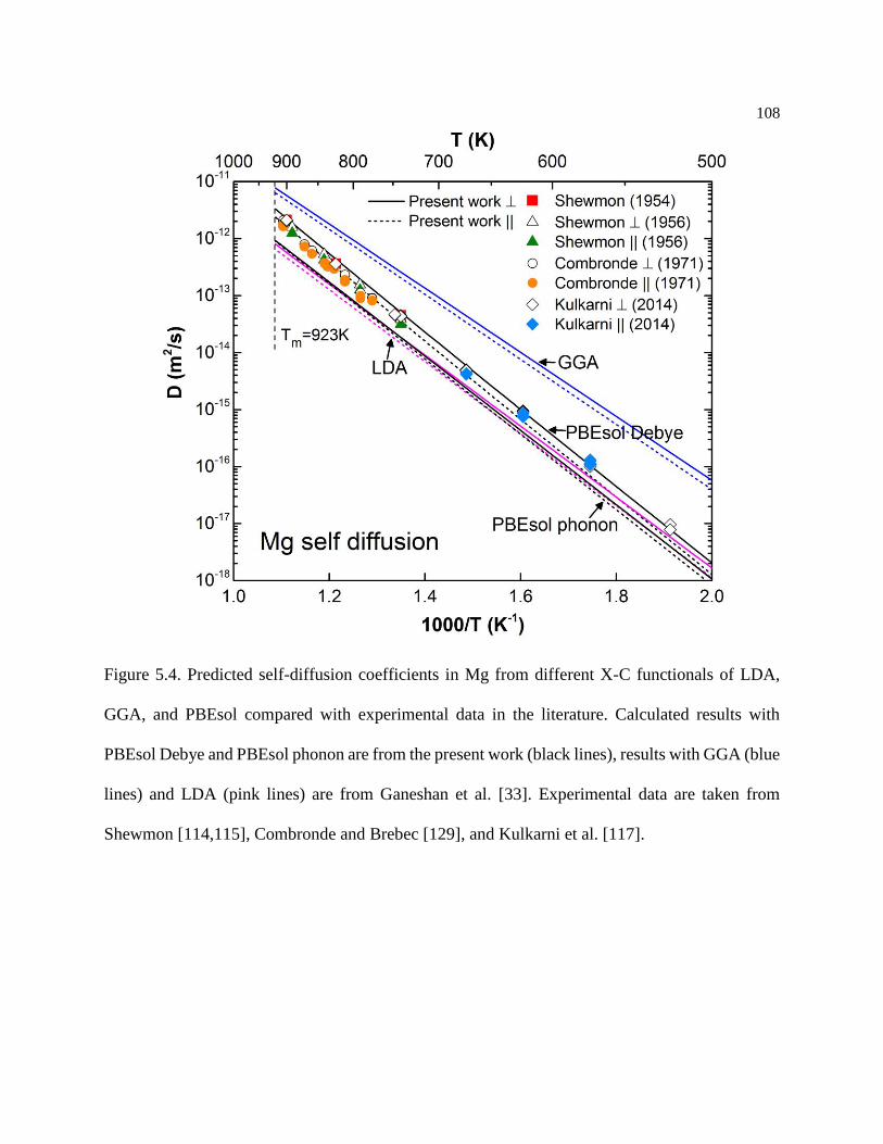
108
Figure 5.4. Predicted self-diffusion coefficients in Mg from different X-C functionals of LDA,
GGA, and PBEsol compared with experimental data in the literature. Calculated results with
PBEsol Debye and PBEsol phonon are from the present work (black lines), results with GGA (blue
lines) and LDA (pink lines) are from Ganeshan et al. [33]. Experimental data are taken from
Shewmon [114,115], Combronde and Brebec [129], and Kulkarni et al. [117].

109
Chapter 6
First-principles predictions of dilute tracer diffusion coefficients of non-rare earth
elements in hcp Mg
6.1 Introduction
In recent years, magnesium (Mg) alloys have received an increasing interest due to their
low density, earth abundance, high specific strength, and good castability [1]. These properties
make Mg alloys attractive for automotive, aerospace, and other light-weight structural applications
[3]. The majority of Mg alloys derives their mechanical properties from precipitation hardening
[9], while the study of precipitation process demands accurate thermodynamic and kinetic
(diffusion) data. Thermodynamics of Mg alloys has been extensively studied, and several
comprehensive thermodynamic databases have been established [10]. However, the kinetics of Mg
alloys has been studied to a far lesser extent, especially diffusion coefficients of various solutes in
Mg. Due to the issues related to corrosion, oxidation, and contamination during sample preparation
in diffusion measurements, few experimental data are available in the literature for diffusion
coefficients of solutes in Mg [5].
For the investigation of kinetic processes in Mg alloys in the solid state, such as creep [15],
solute strengthening [16,17], solution treatment and aging [18], reliable diffusion data and detailed
insights into diffusion of solutes in Mg are desperately needed. For example, the knowledge of
diffusion coefficients can help to determine the desirable aging time to achieve peak hardness in
precipitation-hardened Mg alloys [9]. Wrought Mg alloys have seen very little implementation in

110
the automotive industry because of their poor formability at room temperature [15] as mentioned
before. To improve the formability of wrought Mg alloys, proper alloying additions can be selected
by evaluating their solute drag propensity at the grain boundaries [19] to mitigate the basal plane
texture formation due to the inhomogeneous deformation of hcp Mg. This propensity greatly
depends on their diffusion coefficients based on Cahn’s solute drag theory [11]. Diffusion of
solutes around the dislocation core structure in Mg also plays an important role in understanding
the origin of many plastic phenomena such as dynamic strain aging [17] and plastic instabilities
[20]. Therefore, the information of solute diffusion coefficients in Mg is critical for the
development of new casting and wrought Mg alloys.
Fortunately, it is now possible to calculate many aspects of diffusion [21,22]. First-
principles calculations based on density functional theory (DFT) have been extensively used to
calculate diffusion coefficients, especially when experimental data are lacking [23,24]. These
calculations are usually coupled with transition state theory (TST) under the harmonic or the quasi-
harmonic approximations [22]. TST has become a practical tool in the context of DFT calculations
when efficient algorithms for finding the minimum-energy path have been developed, such as the
nudged elastic band (NEB) and the climb image nudged elastic band (CI-NEB) method [25]. At
present, first-principles calculations of diffusion coefficients are largely limited to cubic systems,
such as those in Al [23,26], Fe [27,28], and Ni [29–31] alloys. This is due to the additional
complexity of anisotropy associated with the calculations of diffusion coefficients in hcp systems.
Recently, Ganeshan et al. [24] in our group calculated the diffusion coefficients of Al, Zn, Sn, and
Ca in dilute hcp Mg using an 8-frequency model. However, their calculated results compared with
experimental data still need to be further improved (see details in Chapter 5 and Chapter 6), and
especially more alloying elements need to be considered for Mg alloys.
111
In the present study, we use first-principles calculations coupled with the TST and the 8-
frequency model to calculate the dilute solute tracer diffusion coefficients in hcp Mg. Forty-seven
substitutional alloying elements have been considered herein, namely Ag, Al, As, Au, Be, Bi, Ca,
Cd, Co, Cr, Cu, Fe, Ga, Ge, Hf, Hg, In, Ir, Li, Mn, Mo, Na, Nb, Ni, Os, Pb, Pd, Pt, Re, Rh, Ru, Sb,
Sc, Se, Si, Sn, Sr, Ta, Tc, Te, Ti, Tl, V, W, Y, Zn, and Zr (see also Figure 6.1). The self-diffusion
coefficient of Mg has been calculated as well. The effects of different exchange-correlation (X-C)
functionals on diffusion properties are examined. It is shown that the recently developed PBEsol
X-C functional [32] yields better agreement with experimental data compared with the commonly
used X-C functionals such as the local density approximation (LDA) and the generalized gradient
approximation (GGA) for the self-diffusion [33] and solute diffusion coefficients (Al, Sn, Zn) in
Mg [24] calculated in previous works. The vibrational properties are derived from the quasi-
harmonic Debye model [34,127]. Therefore, we are able to calculate not only the migration barriers
but also the temperature-dependent jump frequencies and the diffusion pre-factors, which are
related to vibrational entropic contributions. Finally the dilute solute tracer diffusion coefficients
in hcp Mg are calculated. The diffusion pre-factors and the activation energies are obtained by
fitting the calculated diffusion coefficients to the Arrhenius-type diffusion equation (see details in
Section 6.2).
6.2 Diffusion theory
Note that solute diffusion in dilute alloys is also referred to impurity diffusion in the
literature [146]. In the remainder of the paper, “solute” is synonymous with “impurity”. For the
hcp lattice, the crystal anisotropy results in two unique solute jumps, one within the basal plane
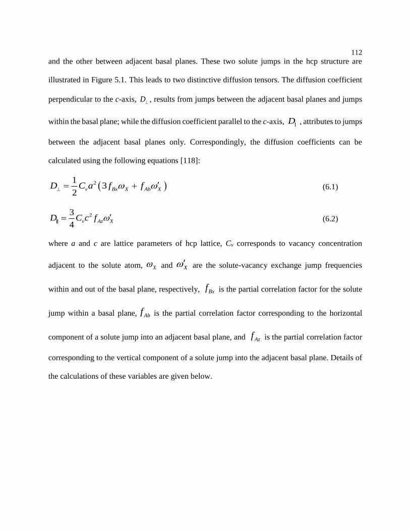
112
and the other between adjacent basal planes. These two solute jumps in the hcp structure are
illustrated in Figure 5.1. This leads to two distinctive diffusion tensors. The diffusion coefficient
perpendicular to the c-axis, D , results from jumps between the adjacent basal planes and jumps
within the basal plane; while the diffusion coefficient parallel to the c-axis, D , attributes to jumps
between the adjacent basal planes only. Correspondingly, the diffusion coefficients can be
calculated using the following equations [118]:
213
2v Bx X Ab XD C a f f
(6.1)
23
4v Az XD C c f (6.2)
where a and c are lattice parameters of hcp lattice, Cv corresponds to vacancy concentration
adjacent to the solute atom, X and X are the solute-vacancy exchange jump frequencies
within and out of the basal plane, respectively, Bxf is the partial correlation factor for the solute
jump within a basal plane, Abf is the partial correlation factor corresponding to the horizontal
component of a solute jump into an adjacent basal plane, and Azf is the partial correlation factor
corresponding to the vertical component of a solute jump into the adjacent basal plane. Details of
the calculations of these variables are given below.

113
6.2.1 Vacancy concentration adjacent to a solute atom
In order for a solute atom to jump, a vacancy adjacent to the solute atom needs to form.
The vacancy concentration adjacent to the solute atom, Cv in Eqs. (6.1) and (6.2) in the dilute limit,
is calculated by a Boltzmann relation:
expf
v
B
GC
k T
(6.3)
where 0
f f bG G G is the free energy of vacancy formation adjacent to the solute atom. 0
fG
is the vacancy formation free energy in pure Mg without solute, as is calculated by
0
1 1
1Mg Va Mgf N N
NG G G
N
(6.4)
where Va indicates a vacancy, and N the number of lattice sites in the supercell. bG is the solute-
vacancy binding free energy, defined as the free energy difference between a solute atom/vacancy
pair and the two as isolated defects [136,147]:
2 1 1 1 1 1 1X Va Mg X Va Mg Mg X Mg Vab N N N NG G G G G (6.5)
where X represents a solute atom. The minus sign in front of bG in Eq. (6.5) is to keep the binding
energy consistent with the convention in the literature such that favorable solute-vacancy binding
is positive [148]. bG shows the effect of solute-vacancy interaction on the vacancy concentration
adjacent to the solute atom. In the course of calculating solute-vacancy binding energy, the dilute
mixing energy mixE for X in hcp Mg solid solution is readily calculated by:
N-1 1 N
1X Mg X Mg Xmix
NE E E E
N
(6.6)
where XE is the total energy of the solute element in its ground state structure.

114
6.2.2 Jump frequencies of solutes
Once a vacancy adjacent to a solute atom is formed, the solute atom has to overcome the
migration barrier to exchange with the vacancy. Based on Eyring’s reaction rate theory [56] of
activated complex, as applied by Wert and Zener [119] to solute diffusion in solids, the solute-
vacancy exchange jump frequencies within and between the basal planes X and X in their
general form can be written as:
exp mB
B
Gk T
h k T
(6.7)
where m TS ISG G G is the solute migration free energy barrier with TSG being the free energy
of the transition state (TS) and ISG the free energy of the initial state (IS). A detailed discussion
of Eq. (6.7) at the high temperature and low temperature ranges is given by Wimmer et al. [120].
Instead of using Vineyard’s harmonic TST [27,121] which requires computation of full phonon
frequencies, we calculate the jump frequency directly from free energy calculations using quasi-
harmonic Debye model as discussed in Section 5.3 Computational details.
6.2.3 Correlation factors and the 8-frequency model
One solute atom can exchange positions with a vacancy and subsequently jump back to its
original position. This results in zero net diffusion distance for the solute atom. The degree to
which this effect hinders diffusion depends on the correlation between two successive solute-
vacancy exchanges, which can be described by a correlation factor f. The correlation factor is a
function of solute and solvent jump frequencies and geometry of crystal lattice. For self-diffusion
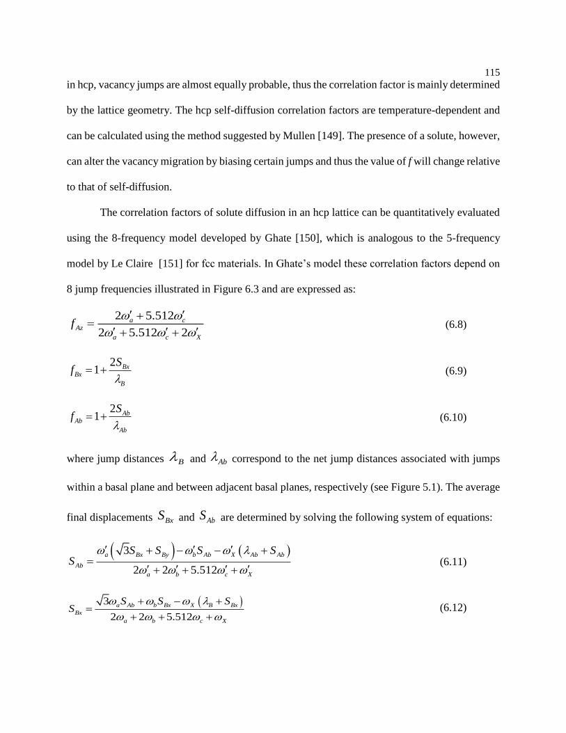
115
in hcp, vacancy jumps are almost equally probable, thus the correlation factor is mainly determined
by the lattice geometry. The hcp self-diffusion correlation factors are temperature-dependent and
can be calculated using the method suggested by Mullen [149]. The presence of a solute, however,
can alter the vacancy migration by biasing certain jumps and thus the value of f will change relative
to that of self-diffusion.
The correlation factors of solute diffusion in an hcp lattice can be quantitatively evaluated
using the 8-frequency model developed by Ghate [150], which is analogous to the 5-frequency
model by Le Claire [151] for fcc materials. In Ghate’s model these correlation factors depend on
8 jump frequencies illustrated in Figure 6.3 and are expressed as:
2 5.512
2 5.512 2
a cAz
a c X
f
(6.8)
21 Bx
Bx
B
Sf
(6.9)
21 Ab
Ab
Ab
Sf
(6.10)
where jump distances B and Ab correspond to the net jump distances associated with jumps
within a basal plane and between adjacent basal planes, respectively (see Figure 5.1). The average
final displacements BxS and AbS are determined by solving the following system of equations:
3
2 2 5.512
a Bx By b Ab X Ab Ab
Ab
a b c X
S S S SS
(6.11)
3
2 2 5.512
a Ab b Bx X B Bx
Bx
a b c X
S S SS
(6.12)
116
2 2 5.512
a Ab b By
By
a b c X
S SS
(6.13)
Using the frequencies of each jump in the 8-frequency model, the Eqs. (6.11)~(6.13) can
be solved and the correlation factors can be calculated using Eqs. (6.8)~(6.10).
Free energies fG and mG can be obtained from DFT calculations based on the quasi-
harmonic approximations described in Section 0 to calculate the jump frequencies X , X , a ,
b , c , a , b , c , and the vacancy concentrations. We then implement them into the 8-
frequency model, and subsequently obtain the diffusion coefficients from Eqs. (6.1) and (6.2). The
calculated diffusion coefficients D in Eqs. (6.1) and (6.2) can be fitted into the conventional
Arrhenius form:
0 expB
QD D
k T
(14)
where Q is the diffusion activation energy and D0 the pre-exponential factor. The activation
energy Q corresponds to the enthalpy of vacancy formation, the enthalpy of solute migration, and
part of the contribution from correlation factors; the diffusion pre-exponential factor D0
corresponds to the entropy of vacancy formation, the entropy of solute migration, the lattice
parameters, and also part of the correlation factors. It should be noted that all the diffusion plots
shown in the present work were plotted using the calculated data directly from first-principles, not
the fitted Arrhenius equation. The original calculated diffusion data set can be found in Ref. [152].

117
6.3 Computational details
First-principles calculations based on DFT were employed to calculate the free energies
needed in the diffusion equations and the 8-frequency model. The ion-electron interaction was
described by the projector augmented plane-wave (PAW) method [48] and the X-C functional was
described by an improved GGA of PBEsol [32], as implemented in the VASP 5.3.2 code [97]. The
suitability of PBEsol for the present study is discussed in the Section 5.4.1 and 5.4.2. An energy
cut-off of 350 eV was used for the plane-wave expansion of the electronic wave functions.
6.3.1 Supercell size and k-point density
Tests were performed on pure Mg and representative solutes Zn and Y to estimate the
convergence of the calculation results with respect to the supercell size and k-point density. On the
basis of these tests, the vacancy formation, migration and binding energies are estimated to be
converged to within a precision of approximately 0.01 eV (see Table 6.1).
After tests of supercell size, we chose a 64-atom supercell (4×4×2 conventional hcp unit
cells) for most solutes, which was sufficient to isolate the vacancy and solute atom from the
periodic images. For Ba, Bi, Ca, K, Pb, Sr, and Y, a 96-atom 4×4×3 supercell was used due to the
large atomic size of these elements. All structural degrees of freedom (ionic coordinates, cell
volume, and cell shape) in the supercell were fully relaxed via a conjugate gradient method to an
energy convergence of 10-5 eV/atom, followed by a final static calculation using the tetrahedron
method with Blöchl corrections [122] with energy convergence of 10-6 eV/atom to get the accurate
total energy. Although constant volume and cell shape were used in other diffusion calculations
[27,123,124], full relaxation of all degrees of freedom can result in more accurate local strain and
118
generate the useful quantity XV , which will be discussed in Section 6.4.1 Solute-vacancy binding
energy. An 8×8×9 -centered k-point mesh was used for the 64-atom supercell for the electronic
integration in the Brillouin zone. For calculations using 96-atom supercells, a 5×5×4 -centered
k-point mesh was used in structural relaxation and a 7×7×7 -centered k-point mesh in subsequent
static calculations.
6.3.2 Transition state search
To determine the position of the saddle point and associated minimum-energy pathway
during solute migration, calculations were performed employing the CI-NEB method [25] with 3
images. The two end-point structures, i.e. the initial and final structures, were fully relaxed first.
The same supercell size and k-point settings were used in the CI-NEB calculations as are
mentioned in the above discussion. Such calculations were performed for all the solute (solvent)-
vacancy exchange in the 8-frequency model for each investigated elements. Unlike hcp Ti (as well
as hcp Zr) with two saddle points [125], in all cases the energy was found to display a single
maximum, corresponding to the saddle point at the high-symmetry position located half way
between neighboring sites.
6.3.3 The quasi-harmonic approach
Vibrational contributions to the free energies were calculated using the quasi-harmonic
approximations from phonon or Debye model. Helmholtz free energy of a configuration as a
function volume (V) and temperature (T) can be expressed as [35]:

119
0( , ) ( ) ( , ) ( , )vib elF V T E V F V T F V T (6.15)
where 0 ( )E V is the static energy at 0 K without the zero-point vibrational energy, ( , )vibF V T
the vibrational contribution, and ( , )elF V T the thermal-electronic contribution. Note that at zero
pressure, the Helmholtz free energy is equal to the Gibbs free energy. In the present work, 0 ( )E V
was calculated via first-principles directly, and ( , )elF V T obtained by integrating the electronic
density of states [98]. It is found that ( , )elF V T has a negligible contribution to the total free energy
compared with ( , )vibF V T , but it was still considered in the present work for the sake of
completeness. Based on the previous work [31] from our group, the quasi-harmonic Debye model
is sufficient to describe well the vibrational contribution to free energy in diffusion calculations
compared with phonon calculations and can save tremendous computing resources. Therefore,
( , )vibF V T for all the initial and transition states were calculated using the quasi-harmonic Debye
model in the present work. We still calculated the self-diffusion coefficients in Mg using quasi-
harmonic phonon model for comparison with the quasi-harmonic Debye model, as shown in Figure
5.4.
In the quasi-harmonic phonon model, the vibrational contribution to Helmholtz energy is
obtained by the integration of calculated phonon density of states. The details of implementation
can be found in our previous works [35,98]. In the quasi-harmonic Debye model [34,35], the
vibrational contribution to Helmholtz energy is described as
9
, 3ln 18
D V
DTvib B D B
VF V T k V k T e D
T
(6.16)
120
where D is the Debye temperature, 9
8B Dk V the zero-point vibrational energy, and Bk the
Boltzmann’s constant. The Debye function, D x , is defined as 3
3
0
3
1
x
z
z dzD x
x e
.
To solve Eq. (6.16), the Debye temperature D must be calculated. In the present work,
the Debye-Grüneisen approximation (Moruzzi-Janak-Schwarz approximation) [53] is used to
describe D :
1/2
1/6 0 00D
B VsAV
M V
(6.17)
where A is a constant, representing 1/3
26 / Bh k , 0V the ground state equilibrium volume, M the
average atomic mass, the Grüneisen parameter, B0 the bulk modulus, and s a parameter that
scales the Debye temperature and depends on the Poisson’s ratio of materials [126]. s=0.69 was
used in the present work to benchmark the Debye temperature of pure Mg (330 K) obtained by the
quasi-harmonic phonon calculations. Excellent agreement was obtained between the
thermodynamic properties (heat capacity±1J/mol, entropy±0.5J/mol/K) calculated from the quasi-
harmonic phonon and Debye model in pure Mg.
Equilibrium properties for input in the Debye model, including volume (V0), energy (E0),
bulk modulus (B0) and its pressure derivative (B0’), were obtained from an energy-volume equation
of state (EOS) calculated from first-principles using the equilibrium volume V0 and at least five
additional volumes (0.96, 0.98, 1.02, 1.04, and 1.06 with respect to V0). A four parameter Birch-
Murnaghan EOS was used herein to fit the energy-volume data. It is represented in its linear form
[35]
2/3 4/3 2( )E V a bV cV dV (6.18)

121
where a, b, c, and d are fitting parameters. This EOS was adopted because it has been previously
shown to be able to produce accurate properties for many materials systems [35,127]. It should be
noted that the EOS for the saddle point configuration was obtained without relaxing each
additional volume in order to maintain its saddle point structure. It is observed that the value of B0’
is quite sensitive to the EOS fitting and is always around 4 in all the EOS fittings. When the fitted
energy-volume curve was not smooth enough due to the scattered energy-volume points which
indicates the B0’ value is far away from 4, the value from a pressure-volume fitting [128] was used
instead.
6.4 Results and Discussion
6.4.1 Solute-vacancy binding energy
The binding energies of solute-vacancy pairs in Mg modify the vacancy concentration
adjacent to the solute atom and have been reported in Table 6.2. The present DFT results show a
good agreement with those calculated by Shin et al. [136] using GGA as the X-C functional. A
positive sign on the solute-vacancy binding energies indicates favorable binding (attractive) while
negative sign indicates unfavorable binding (repulsive). Vydyanath et al. [153] and Rao and
Suryanarayana [154] measured the vacancy-binding energies of Zn and Al in Mg, respectively,
both from quenching experiments as shown in Table 6.2. There is a large discrepancy between the
measured 0.29 eV [154] and the calculated 0.02 eV for Al-vacancy binding in Mg, which may be
due to inaccuracies of non-equilibrium measurements. The measured Zn-vacancy binding energy
of 0.07 eV in Mg [153] is in good agreement with the calculated 0.05 eV in the present work.

122
For a quantitative measure of the atomic size of each solute X, the volume difference XV
induced by placing a single solute into pure Mg is calculated and shown in Table 6.2, which is
expressed as [124]:
1 1Mg X MgX N NV V V (6.19)
Except for transition metals (TMs), modest correlation is found between solute-vacancy
binding energy and XV . This correlation can be explained by a simple strain model proposed by
Shin [136]. It states that a large solute atom in Mg will induce a significant strain on the
surrounding Mg atoms, and a vacancy adjacent to such a large solute atom will allow the solute
atom to relax towards the vacancy and relieve the strain. Therefore for solutes with large atomic
size, large solute-vacancy binding energies are obtained due to the large induced strain, such as Sr
(0.30 eV), K (0.40 eV), and Ba (0.67 eV).
However, this strain model does not explain the binding behavior of TMs in Mg. Figure
6.4 shows the solute-vacancy binding energies of various solutes within the basal plane. Early TMs,
e.g. Ti, V, Cr, and Mn for 3d metals, have unfavorable binding with vacancy in Mg, while late
TMs, e.g. Fe, Co, Ni, Cu, and Zn for 3d metals, have favorable binding with vacancy in Mg. The
solute-vacancy binding energies follow the similar trend as a function of atomic number for 3d,
4d, and 5d TMs, exhibiting a flatwise “S” shape curve in Figure 6.4. Simonovic and Sluiter [123]
also found that TMs in Al bind with vacancies in a similar manner.
Solutes with strong vacancy binding might strongly affect the precipitation behavior of
other alloying elements because of vacancy trapping after the solutionizing heat treatment [9]. For
example, the very strong vacancy binding of Sr causes a significant decrease of the vacancy
formation energy adjacent to a Sr solute and may result in vacancy trapping. However, the Mg-Sr
123
system has very positive enthalpy of mixing in the hcp phase [79], causing Sr to be repelled from
Mg atoms. Therefore, the Sr atom forms a complex with a vacancy in which the Sr atom is
displaced toward the vacancy to relieve the strain. The barrier for Sr-vacancy exchange XE is
extremely low (0.01 eV) because the Sr atom sits almost at the midpoint between two sites. The
same situation also applies to K and Ba, for which the solute-vacancy binding becomes so strong
that their migration barriers are vanishingly small.
6.4.2 Effects of X-C functionals
Table 6.4 summarizes the calculated diffusion coefficients for various solutes in Mg
compared with available experiments [76-88]. In many experiments, the measured diffusion
coefficient data points were few and scattered, and the fitted values of activation energy Q and
diffusion pre-factor D0 have relatively large error bars. For solutes with more measurements
available in the literature, such as Al [83-85, 88], Zn [77, 82, 86, 88], and Sn [155], the present
predictions agree remarkably well with experimental values within a factor of 3, as shown in Figure
6.7. Solute diffusion results of Al, Zn, and Sn from LDA [24] show slopes compare well with
experiments but consistently underestimate intersects of diffusion coefficients (D0), as seen in
Figure 6.7. This can be understood by similar analysis discussed in Section 5.4.2 for Mg self-
diffusion due to the overbinding of LDA. Figure 6.8 shows all of the basal dilute solute tracer
diffusion coefficients in hcp Mg calculated in the present work. A large spectrum of values of
diffusion coefficients across more than 10 orders of magnitude is found in solute diffusion in hcp
Mg. More calculated diffusion coefficients compared with available experiments can be found in
Refs. [40][156] as well as illustrated in Figure 6.12~Figure 6.21.
124
6.4.3 Effects of correlation
From Eqs. (6.1) and (6.2), it is seen that the diffusion coefficients are linearly dependent
on the correlation factors, which can range from 0 to 1. If correlation effects are weak, the
correlation factors can be ignored because their values are close to 1. They will have little effects
on the final calculated diffusion coefficients, as shown by Ganeshan et al. [24] for Al, Zn, and Sn
diffusions in Mg. However, if the correlation effects are strong, the correlation factors become
small and greatly decrease the calculated diffusion coefficients. For examples, the calculated
correlation factors of Ca and Zn diffusion in Mg as a function of temperature are shown in Figure
6.5(b). Correlation factors of Zn are all above 0.9, while correlation factors of Ca are all below
0.25. Interestingly, the correlation factors of Ca increases as the temperature increases while those
of Zn show the opposite trend. Figure 6.5(a) shows the calculated diffusion coefficients of Ca and
Zn in Mg with and without correlation effects considered. Diffusion coefficients of Ca with and
without correlation differ around one order of magnitude, showing non-negligible effects of
correlation. Diffusion coefficients of Zn with and without correlation almost overlap with each
other in Figure 6.5(a), showing little effects of correlation. More diffusion plots showing
comparisons with and without correlation effects considered can be found in Section 3.1 and 3.2
in Ref. [40].
The correlation effects can be further understood by the migration barriers of each jump in
the 8-frequency model. Table 6.3 lists the energy barriers of vacancy migration for solutes Zn, Pb,
Bi, Ca, Na, Se, Sr, Te, and Y in Mg. As shown in Table 6.3, the direct solute migration barriers
( XE and XE ) for Zn and Pb are larger than the other solvent (Mg) migration barriers ( aE , bE ,
cE , aE , bE , and cE ). While for the elements with strong correlation effects, i.e. Ca, Sr, Y, Na,

125
Se, and Te, the direct solute migration barriers are significantly smaller than the solvent migration
barriers. For example, the direct Sr migration barriers, XE =0.01 eV and XE =0.02 eV, are
extremely small due to the strong solute-vacancy binding mentioned in Section 6.4.1. The small
direct solute migration barriers lead to fast solute-vacancy oscillations which do not themselves
contribute to the net diffusion. This large difference between the direct solute migration barriers
and the solvent migration barriers is the origin of the strong correlation effects of these solutes.
The elements with much bigger direct solute migration barriers than the solvent migration barriers,
such as the transition metals, have very weak correlation effects. Therefore, the six solvent (Mg)
atoms jump frequencies ( a , b , c , a , b , c ) for elements other than Ca, Na, Se, Sr, Te,
and Y were not calculated in this work because they don’t contribute to the final diffusion
coefficients significantly. For Bi, it behaves almost like Mg self-diffusion because all of the
migration barriers are close to 0.44 eV. The present study also confirms that 8-frequency model is
sufficient to capture the correlation effects of solute diffusion in hcp Mg in a quantitative level.
A very good indicator of the correlation effects is the volume difference XV induced by
placing a single solute into pure Mg as discussed by Huber et al. [45]. Solutes with small or
negative XV , like ZnV =-11.1 Å3/supercell, show weak correlation effects, indicating the
correlation factors for the diffusion of these solutes in Mg to be very close to 1. Solutes with large
positive XV such as Ca, Na, Sr, Te, and Y show strong correlation effects in diffusion, indicating
the correlation factors in these systems to be much less than 1 and showing non-negligible effects
on the calculated diffusion coefficients. The effects of XV can be traced back to their migration
barriers. Large atomic size induces large lattice misfit strain and causes large positive XV , which
126
leads to more local free space and thus lower XE for solutes like Ca, Na, Sr, Te, and Y, as shown
in Figure 6.6. This indicates that the larger solute atoms can move faster while the smaller ones
move slower. Interestingly, Se is an exception. Even with a negative XV (-4.6 Å3), the migration
barriers of Se are very small (e.g. XE =0.08 eV). This may be due to the fact that, unlike those
solutes with large atomic size, the atomic size of Se (1.03 Å) is the smallest among all the solutes
studied herein and is much smaller than that of Mg (1.45 Å), which can also give Se more free
space to move in the Mg lattice.
6.4.4 Bonding and trends in calculated diffusion data
As can be seen in Figure 3.4, the activation energy vs. atomic number curves show an
inverse “V” shape, indicating the TM solutes have large activation energy. This may due to the
strong interaction between solute atoms with d electrons and the Mg matrix, which is traceable
from the larger bulk moduli of these metals (see Table 6.2 and Figure 6.10). In an effort to seek
the diffusivity trend, Figure 6.10 shows the basal diffusion coefficients of various solutes at 800
K as a function of bulk modulus for the Mg63X alloys (Mg95X for Bi, Ca, Pb, Sr, and Y). Bulk
modulus represents the bonding strength between the solute atom and Mg matrix. Higher bulk
modulus indicates stronger bonding between solute atom and Mg matrix and less mobile solute
atom in the Mg matrix, resulting in a decreasing diffusion coefficient as the value of bulk modulus
increases. In addition, the smaller solute atoms such as Re and W exhibit lower diffusivities in Mg
due to their larger bulk moduli (see Figure 6.10). These observations are consistent with the
conclusion drawn for solute diffusion in Ni-based alloys [21]. Most early TMs, such as Ti, V, Cr,
Mn, Fe, Ni, Zr, and Hf, do not form favorable bonds with Mg. In binary Mg-X alloy systems with

127
these elements, no ordered intermetallic compounds are experimentally observed. These alloying
elements in hcp Mg also tend to have positive enthalpies of mixing ( mixE >0), often indicating an
energetic preference for phase separation and limited solid solubility, as shown in Table 6.2.
As, Ca, Ga, Hg, Li, Na, Sb, Se, Sr, Te, Tl, and Zn are faster diffusers than Mg self-diffusion,
while other solutes diffuse slower than Mg self-diffusion. Solutes which have high diffusion
coefficients and low solid solubility, such as Ca, Na, Sb, and Sr, may serve as good alloying
candidates for texture refinement since they have a high tendency to segregate to the grain
boundaries and pin the grain boundary movement. The comparison between first-principles
predicted diffusion coefficients and other solutes with experimental data are shown in Figure
6.12~Figure 6.21.
Although solute diffusion in Mg is anisotropic, the difference between values of D and
D is usually not very large since atomic migration is a local phenomenon. The ratio D / D is
within a factor of 5 for most solutes, as shown in Figure 6.11. Note also that of all the
experimentally measured solute diffusion coefficients, D is larger than D , with the exception
being for Ag diffusion in Mg. The diffusion coefficient D of Ag in Mg is smaller than D from
the experiments by Combronde and Brebec [79] (see Figure 6.12). The calculated diffusion
coefficients differ with experimental data by one order of magnitude. Further experimental and
computational work need to be done to elucidate this discrepancy. Meanwhile, for big solute atoms
like Ba and K, the CI-NEB predicts that the saddle point configuration between the solute and
vacancy sites is more stable than the initial configurations. Thus the diffusion coefficients in Mg
for large solutes, Ba, K, Rb, and Cs could not be calculated in terms of transition state theory.

128
6.5 Conclusions
As an effort for computational and data-driven development of advanced Mg-based alloys,
we present a comprehensive study of dilute solute diffusion coefficients of 47 substitutional
alloying elements in hcp Mg. The 8-frequency model for solute diffusion within an hcp lattice has
been used to compute the correlation factors for different jumps. All the energies and vibrational
quantities required to compute the jump frequencies and hence derive the solute diffusion
coefficients from the 8-frequency model are calculated with the DFT based first-principles
calculations in terms of the X-C functional of PBEsol and the quasi-harmonic Debye model.
Saddle point configurations are predicted using the first-principles based CI-NEB method. It is
found that:
(1) Compared with LDA and GGA, PBEsol is able to well describe both vacancy formation
energies and vibrational properties, resulting in more accurate quantitative predictions of
diffusion coefficients.
(2) Correlation effects are not negligible in solutes Ca, Na, Se, Sr, Te, and Y, in which the
direct solute migration barriers are significantly smaller than the solvent migration barriers.
This indicates that the larger solute atoms can move faster while the smaller ones move
slower, with the exception of Se.
(3) The solute diffusion coefficients in hcp Mg are roughly inversely proportional to bulk
modulus, i.e. their bonding to Mg. Transition metal elements with d electrons strongly
interact with Mg and have very large diffusion activation energies, which cannot be
explained by a simple strain model based on atomic size.
(4) The predicted solute diffusion coefficients in Mg compare remarkably well with available
experiments in the literature. For most solutes basal diffusion coefficients are bigger than
129
the non-basal ones. The diffusion coefficient of Ag shows anomaly with basal and non-
basal diffusion coefficients showing opposite trend compared with other alloying elements.
(5) The present work lays the foundation of diffusion data for future rational design of novel
casting and wrought Mg alloys. The calculated diffusion data can be used to develop
CALPHAD-type diffusion mobility databases for multi-component Mg alloys [14]. The
theoretical methodology used herein can be readily applied to solute diffusion in other hcp
systems.

130
Table 6.1 Supercell size convergence of basal and normal solute-vacancy binding energies for Zn and Y. basal
bindE and normal
bindE are the solute-vacancy binding energies of solute and vacancy on the same basal plane
and between adjacent basal planes of hcp Mg, respectively.
Solute Solute-vacancy binding energy (eV)
36 atoms 64 atoms 96 atoms 150 atoms
Zn basal
bindE
0.065 0.054 0.055
normal
bindE
0.047 0.038 0.039
Y basal
bindE
-0.112 -0.081 -0.051 -0.051
normal
bindE
-0.096 -0.065 -0.055 -0.045
Note: the solute-vacancy binding energies listed here were obtained from full structural relaxations without
static calculations. For accurate values of solute-vacancy binding energies in Mg, the reader should refer to
Table 6.2.

131
Table 6.2 First-principles predicted properties of solutes in hcp Mg by the X-C functional of PBEsol,
including the volume difference, bulk modulus, solute-vacancy binding energies and migration barriers.
Here, XV indicates the volume difference induced by placing a single solute into pure Mg, see Eq.(6.19)
. B is the bulk modulus of Mg63X (Mg95X for Ba, Bi, Ca, K, Pb, Sr, and Y). basal
bindE and normal
bindE are the
solute-vacancy binding energies of solute and vacancy on the same basal plane and between adjacent basal
planes of hcp Mg, respectively. XE and XE are the solute migration barriers for solute-vacancy exchange
within the basal plane and between adjacent basal planes, respectively. mixE is the dilute mixing energy
given in units of eV per atom of solute. S is the maximum solid solubility of each element in Mg from
experiments [157].
Solute XV (Å3) B (GPa) basal
bindE (eV) normal
bindE (eV) XE (eV) XE (eV) mixE (eV/sol) S (at.%)
Mg 0 37.9 - - 0.41 0.44 - -
Ag -13.3 38.6 0.05 0.04 0.63 0.68 -0.33 2.58
Al -7.8 38.3 0.02a 0.02 0.46 0.48 0.12 11.8
As -9.4 38.5 0.15 0.15 0.44 0.45 -0.49 ~0
Au -17.8 39.0 0.12 0.08 0.77 0.82 -1.12 0.1
Ba 34.0 36.8 0.67 0.58 0 0 0.76 0.002
Be -16.3 38.4 0.09 0.06 0.57 0.58 1.31 N/Ac
Bi 6.9 38.2 0.11 0.12 0.44 0.44 -0.39 1.12
Ca 15.1 37.3 0.08 0.10 0.14 0.18 0.03 0.44
Cd -5.0 38.3 0.05 0.04 0.46 0.49 -0.28 100
Co -26.1 38.6 0.17 0.07 1.27 1.34 1.04 ~0
Cr -12.0 38.4 -0.08 -0.09 0.81 0.84 1.34 N/A
Cu -18.0 38.6 0.10 0.06 0.65 0.67 0.35 0.234
Fe -20.4 38.5 0.03 -0.02 0.96 1.02 1.30 0.00043
Ga -9.1 38.2 0.06 0.05 0.49 0.52 -0.23 3.14
Ge -9.6 38.4 0.09 0.08 0.56 0.61 -0.20 0.003
Hf -3.3 38.7 -0.26 -0.26 0.82 0.92 0.76 ~0
Hg -7.3 38.4 0.07 0.06 0.45 0.48 -0.68 1.2
In -1.4 38.2 0.06 0.06 0.47 0.49 -0.35 19.4
Ir -30.0 39.7 0.19 0.10 1.67 1.63 -0.59 ~0
K 25.5 36.7 0.40 0.37 0 0 1.28 ~0
Li -4.4 37.5 0.003 ~0 0.36 0.39 -0.16 17
Mn -14.0 38.3 -0.06 -0.07 0.74 0.81 0.96 0.996
Mo -19.4 39.2 -0.18 -0.21 1.54 1.68 1.61 ~0
Na 7.1 37.0 0.08 0.08 0.18 0.19 0.38 0.5
Nb -11.9 39.0 -0.28 -0.29 1.19 1.33 1.23 ~0
Ni -24.3 38.8 0.17 0.08 1.03 1.07 0.35 <0.04
Os -29.6 39.7 0.10 0.01 1.91 1.80 0.88 N/A
Pb 4.4 37.9 0.08 0.09 0.44 0.45 -0.26 7.75
Pd -22.4 39.1 0.13 0.07 1.04 1.11 -1.17 <0.23
Pt -26.3 39.4 0.20 0.12 1.26 1.31 -1.54 ~0
Re -26.1 39.6 -0.05 -0.11 1.91 1.86 1.69 N/A
Rh -27.3 39.4 0.15 0.07 1.44 1.49 -0.77 N/A
Ru -27.9 39.5 0.09 0.01 1.68 1.70 0.35 N/A
Sb 1.2 38.3 0.12 0.13 0.45 0.48 -0.51 <0.04
Sc 1.2 38.2 -0.16 -0.14 0.50 0.58 -0.05 29
Se -4.6 38.2 0.26 0.26 0.08 0.07 -0.86 N/A
Si -12.7 38.6 0.09 0.08 0.61 0.66 0.29 0.005
Sn -0.2 38.2 0.08 0.08 0.52 0.55 -0.46 3.35
Sr 22.5 37.1 0.30 0.29 0.01 0.02 0.44 0.03

132
Ta -12.4 39.1 -0.29 -0.30 1.27 1.41 1.67 N/A
Tc -24.4 39.4 -0.04 -0.10 1.71 1.78 1.07 N/A
Te 5.3 38.0 0.20 0.22 0.18 0.19 -0.57 N/A
Ti -8.9 38.7 -0.21 -0.22 0.84 0.95 0.79 0.12
Tl 1.6 37.9 0.04 0.04 0.39 0.40 -0.29 15.4
V -11.8 38.6 -0.14 -0.15 0.90 1.00 1.32 ~0
W -19.7 39.3 -0.20 -0.23 1.68 1.77 2.29 N/A
Y 11.5 37.9 -0.07 -0.06 0.28 0.33 -0.06 4.7
Zn -11.1 38.2 0.05b 0.04 0.46 0.48 0.05 2.5
Zr -2.1 38.6 -0.25 -0.24 0.76 0.86 0.37 1.042 a Experimental bindE Al Va =0.29±0.02 eV [154]
b Experimental bindE Zn Va =0.07±0.02 eV [153]
c N/A indicates that experiments of solid solubility in Mg are not available in the literature.

133
Table 6.3 Energy barriers (eV) of vacancy migration for various solutes in hcp Mg. The subscripts refer to
the migration pathways indicated in Figure 6.3.
Solute XE XE
aE aE
bE bE
cE cE
Zn 0.46 0.48 0.27 0.26 0.38 0.27 0.44 0.42
Pb 0.45 0.46 0.40 0.45 0.42 0.41 0.45 0.43
Bi 0.44 0.44 0.47 0.48 0.43 0.43 0.45 0.43
Ca 0.14 0.18 0.73 0.75 0.55 0.70 0.37 0.37
Na 0.18 0.19 0.55 0.56 0.48 0.52 0.40 0.40
Se 0.08 0.07 0.34 0.35 0.45 0.38 0.47 0.42
Sr 0.01 0.02 0.96 0.95 0.76 0.90 0.47 0.43
Te 0.18 0.19 0.48 0.50 0.45 0.44 0.49 0.46
Y 0.28 0.33 0.67 0.68 0.47 0.63 0.33 0.34
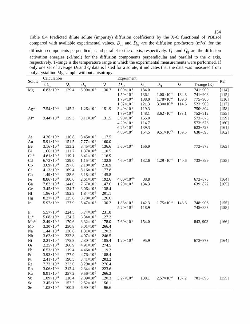
134
Table 6.4 Predicted dilute solute (impurity) diffusion coefficients by the X-C functional of PBEsol
compared with available experimental values. 0D
and 0D are the diffusion pre-factors (m2/s) for the
diffusion components perpendicular and parallel to the c axis, respectively. Q and Q are the diffusion
activation energies (kJ/mol) for the diffusion components perpendicular and parallel to the c axis,
respectively. T-range is the temperature range in which the experimental measurements were performed. If
only one set of average D0 and Q data is listed for a solute, it indicates that the data was measured from
polycrystalline Mg sample without anisotropy.
Solute Calculation Experiment
Ref. 0D
Q
0D Q 0D
Q
0D Q T-range (K)
Mg 6.83×10⁻⁵ 129.4 5.90×10⁻⁵ 130.7 1.00×10⁻⁴ 134.0 741~900 [114]
1.50×10⁻⁴ 136.1 1.00×10⁻⁴ 134.8 741~908 [115]
1.75×10⁻⁴ 138.0 1.78×10⁻⁴ 139.0 775~906 [116]
1.32×10⁻⁵ 121.3 3.30×10⁻⁶ 114.6 523~900 [117]
Ag* 7.54×10-5 145.2 1.26×10⁻⁴ 151.9 3.40×10⁻⁵ 119.3 750~894 [158]
1.79×10⁻³ 148.1 3.62×10⁻⁴ 133.1 752~912 [155]
Al* 3.44×10-5 129.3 3.11×10⁻⁵ 131.5 3.90×10⁻³ 155.0 573~673 [159]
4.20×10⁻⁷ 114.7 573~673 [160]
6.25×10⁻⁵ 139.3 623~723 [161]
4.86×10⁻³ 154.5 9.51×10⁻³ 159.5 638~693 [162]
As 4.36×10⁻⁵ 116.8 3.45×10⁻⁵ 117.5
Au 5.91×10⁻⁵ 151.5 7.77×10⁻⁵ 160.0
Be 3.16×10⁻⁵ 133.2 3.45×10⁻⁵ 136.6 5.60×10⁻⁴ 156.9 773~873 [163]
Bi 1.66×10⁻⁶ 111.7 1.37×10⁻⁶ 110.5
Ca* 4.61×10-4 119.1 3.41×10⁻⁴ 116.9
Cd 6.72×10⁻⁵ 129.0 1.15×10⁻⁴ 132.8 4.60×10⁻⁵ 132.6 1.29×10⁻⁴ 140.6 733~899 [155]
Co 3.69×10⁻⁵ 197.8 2.10×10⁻⁵ 210.9
Cr 4.13×10⁻⁵ 169.4 8.16×10⁻⁵ 177.8
Cu 1.49×10⁻⁵ 138.6 3.18×10⁻⁵ 145.8
Fe 8.86×10⁻⁵ 180.6 2.61×10⁻⁴ 192.6 4.00×10⁻¹⁰ 88.8 673~873 [164]
Ga 7.82×10⁻³ 144.0 7.67×10⁻³ 147.6 1.20×10⁻⁴ 134.3 639~872 [165]
Ge 3.45×10⁻⁵ 134.7 3.06×10⁻⁵ 138.4
Hf 1.86×10⁻⁵ 192.5 1.84×10⁻⁵ 201.1
Hg 8.27×10⁻⁵ 125.8 3.78×10⁻⁵ 126.6
In 5.97×10⁻⁵ 127.9 5.47×10⁻⁵ 130.2 1.88×10⁻⁴ 142.3 1.75×10⁻⁴ 143.3 748~906 [155]
5.20×10⁻⁶ 118.9 745~883 [158]
Ir 5.57×10⁻⁶ 224.5 5.74×10⁻⁶ 231.8
Li* 5.08×10-5 124.2 6.34×10⁻⁵ 127.2
Mn* 2.49×10-4 170.6 3.32×10⁻⁴ 178.0 7.60×10⁻⁵ 154.0 843, 903 [166]
Mo 3.30×10⁻⁶ 250.8 5.01×10⁻⁶ 266.4
Na 1.44×10⁻⁴ 120.8 1.31×10⁻⁴ 120.3
Nb 3.62×10⁻⁵ 232.8 4.97×10⁻⁵ 246.5
Ni 2.21×10⁻⁴ 175.8 2.30×10⁻⁴ 185.4 1.20×10⁻⁹ 95.9 673~873 [164]
Os 2.25×10⁻³ 266.9 4.91×10⁻³ 274.5
Pb 6.53×10⁻⁶ 119.4 4.46×10⁻⁶ 119.2
Pd 3.93×10⁻⁵ 177.0 4.76×10⁻⁵ 188.4
Pt 2.41×10⁻⁵ 190.5 3.41×10⁻⁵ 203.2
Re 7.73×10⁻⁶ 273.0 8.29×10⁻⁶ 276.4
Rh 3.06×10⁻⁵ 212.4 2.34×10⁻⁵ 223.6
Ru 8.91×10⁻³ 257.2 9.56×10⁻³ 266.2
Sb 1.89×10⁻⁵ 118.4 2.09×10⁻⁵ 120.3 3.27×10⁻⁴ 138.1 2.57×10⁻⁴ 137.2 781~896 [155]
Sc 3.45×10⁻⁵ 152.2 2.52×10⁻⁵ 156.1
Se 1.05×10⁻⁴ 100.2 6.90×10⁻⁵ 96.6
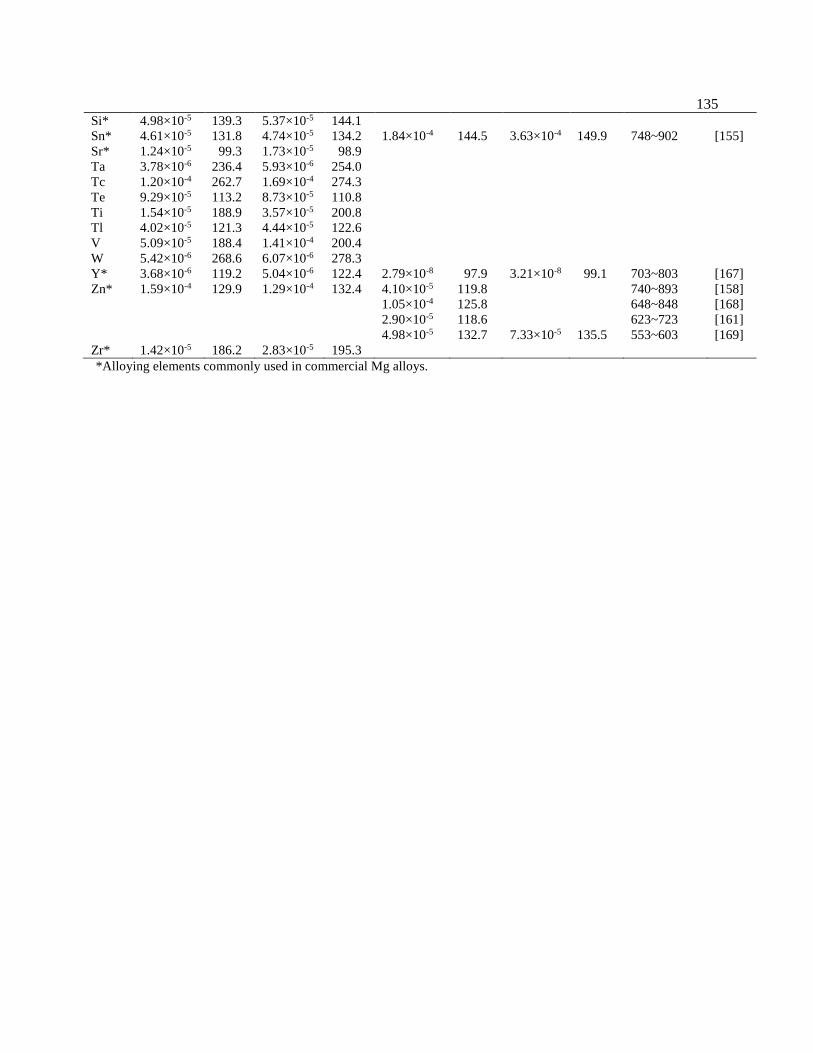
135
Si* 4.98×10-5 139.3 5.37×10⁻⁵ 144.1
Sn* 4.61×10-5 131.8 4.74×10⁻⁵ 134.2 1.84×10⁻⁴ 144.5 3.63×10⁻⁴ 149.9 748~902 [155]
Sr* 1.24×10-5 99.3 1.73×10⁻⁵ 98.9
Ta 3.78×10⁻⁶ 236.4 5.93×10⁻⁶ 254.0
Tc 1.20×10⁻⁴ 262.7 1.69×10⁻⁴ 274.3
Te 9.29×10⁻⁵ 113.2 8.73×10⁻⁵ 110.8
Ti 1.54×10⁻⁵ 188.9 3.57×10⁻⁵ 200.8
Tl 4.02×10⁻⁵ 121.3 4.44×10⁻⁵ 122.6
V 5.09×10⁻⁵ 188.4 1.41×10⁻⁴ 200.4
W 5.42×10⁻⁶ 268.6 6.07×10⁻⁶ 278.3
Y* 3.68×10-6 119.2 5.04×10⁻⁶ 122.4 2.79×10⁻⁸ 97.9 3.21×10⁻⁸ 99.1 703~803 [167]
Zn* 1.59×10-4 129.9 1.29×10⁻⁴ 132.4 4.10×10⁻⁵ 119.8 740~893 [158]
1.05×10⁻⁴ 125.8 648~848 [168]
2.90×10⁻⁵ 118.6 623~723 [161]
4.98×10⁻⁵ 132.7 7.33×10⁻⁵ 135.5 553~603 [169]
Zr* 1.42×10-5 186.2 2.83×10⁻⁵ 195.3
*Alloying elements commonly used in commercial Mg alloys.
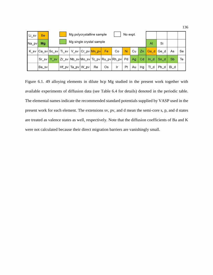
136
Figure 6.1. 49 alloying elements in dilute hcp Mg studied in the present work together with
available experiments of diffusion data (see Table 6.4 for details) denoted in the periodic table.
The elemental names indicate the recommended standard potentials supplied by VASP used in the
present work for each element. The extensions sv, pv, and d mean the semi-core s, p, and d states
are treated as valence states as well, respectively. Note that the diffusion coefficients of Ba and K
were not calculated because their direct migration barriers are vanishingly small.

137
Figure 6.2 Energy convergence as a function of KPOINTS for (a) a 64 atom supercell (b) a 96
atom supercell.

138
Figure 6.3. Illustration of the eight possible vacancy exchanges in an hcp lattice for vacancy and
solute starting (a) within the basal plane and (b) between adjacent basal planes. X , X are the
jump frequencies for the solutes (X) and a , b , c , a , b , c are the jump frequencies
for the solvents (Mg).
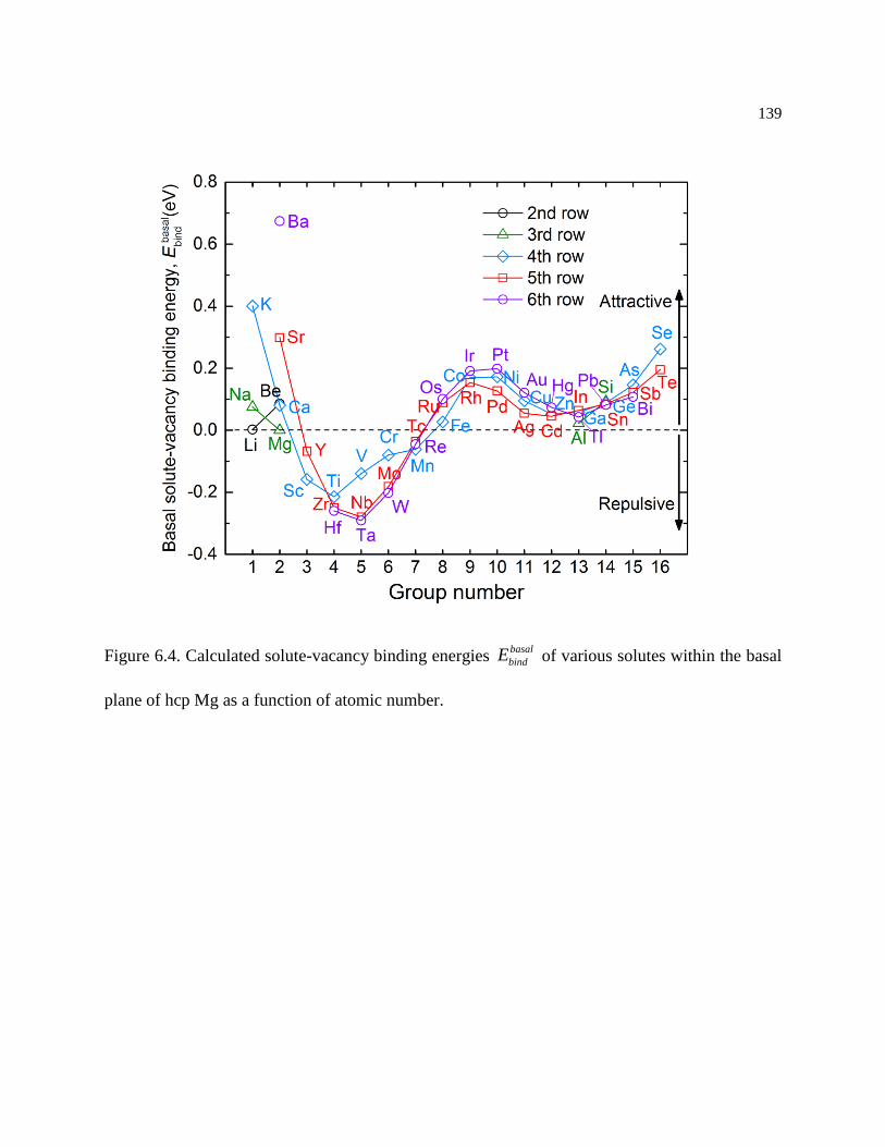
139
Figure 6.4. Calculated solute-vacancy binding energies basal
bindE of various solutes within the basal
plane of hcp Mg as a function of atomic number.
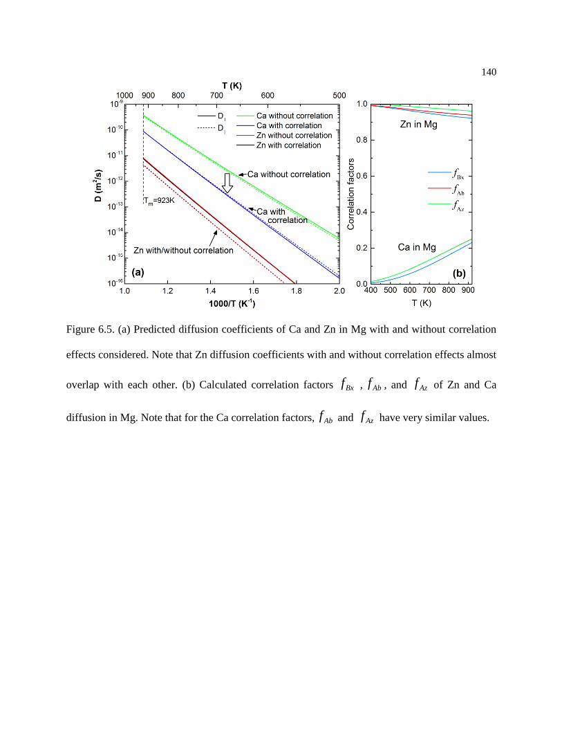
140
Figure 6.5. (a) Predicted diffusion coefficients of Ca and Zn in Mg with and without correlation
effects considered. Note that Zn diffusion coefficients with and without correlation effects almost
overlap with each other. (b) Calculated correlation factors Bxf , Abf , and Azf of Zn and Ca
diffusion in Mg. Note that for the Ca correlation factors, Abf and Azf have very similar values.
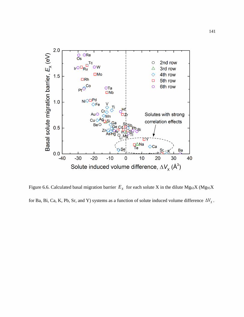
141
Figure 6.6. Calculated basal migration barrier XE for each solute X in the dilute Mg63X (Mg95X
for Ba, Bi, Ca, K, Pb, Sr, and Y) systems as a function of solute induced volume difference XV .
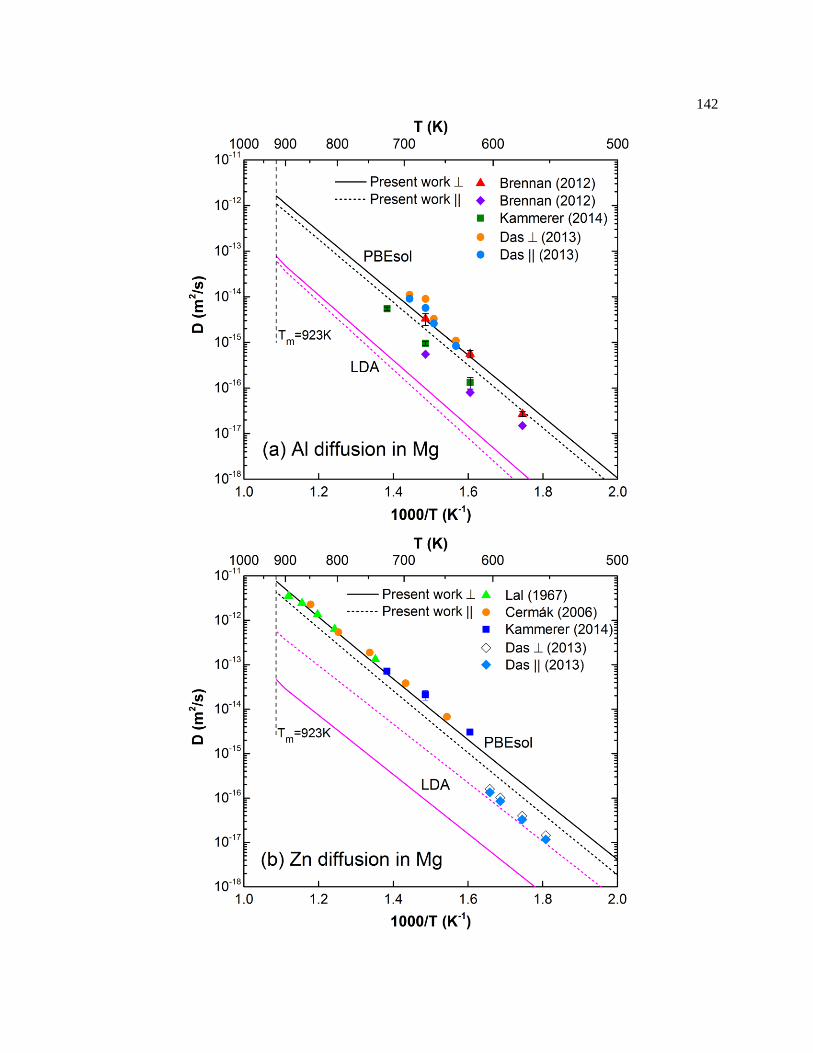
142
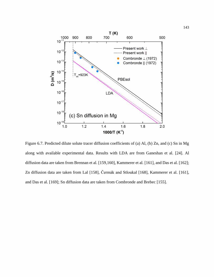
143
Figure 6.7. Predicted dilute solute tracer diffusion coefficients of (a) Al, (b) Zn, and (c) Sn in Mg
along with available experimental data. Results with LDA are from Ganeshan et al. [24]. Al
diffusion data are taken from Brennan et al. [159,160], Kammerer et al. [161], and Das et al. [162];
Zn diffusion data are taken from Lal [158], Čermák and Stloukal [168], Kammerer et al. [161],
and Das et al. [169]; Sn diffusion data are taken from Combronde and Brebec [155].
144
Figure 6.8. Predicted basal dilute solute tracer diffusion coefficients D of 47 solutes in hcp Mg.
The basal self-diffusion coefficient of Mg is plotted in a dashed line.

145
Figure 6.9. Calculated activation energies Q of basal diffusion coefficients of various solutes in
Mg as a function of atomic number, see Table 3.3 for values.
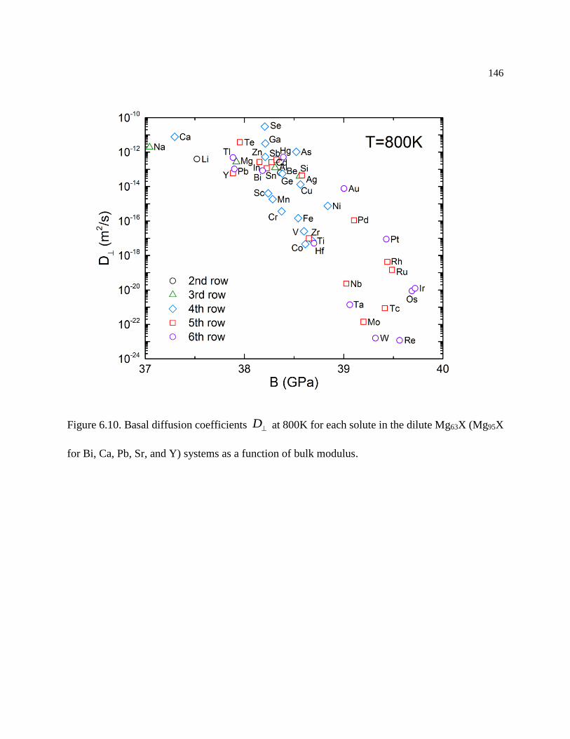
146
Figure 6.10. Basal diffusion coefficients D at 800K for each solute in the dilute Mg63X (Mg95X
for Bi, Ca, Pb, Sr, and Y) systems as a function of bulk modulus.

147
Figure 6.11. The ratio of predicted basal dilute solute diffusion coefficient over the non-basal one,
D/ D , for 47 solutes in hcp Mg. The ratio of self-diffusion coefficients of Mg is plotted in a
dashed line.
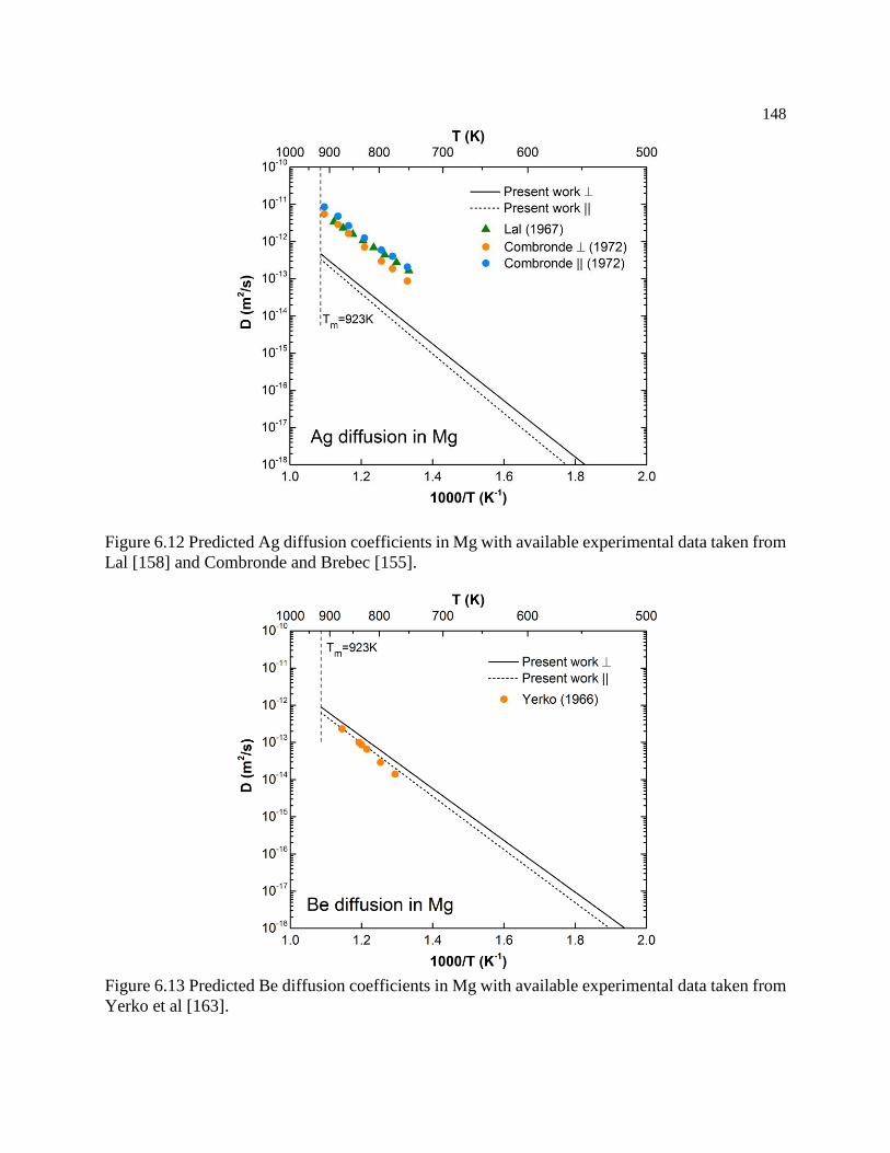
148
Figure 6.12 Predicted Ag diffusion coefficients in Mg with available experimental data taken from
Lal [158] and Combronde and Brebec [155].
Figure 6.13 Predicted Be diffusion coefficients in Mg with available experimental data taken from
Yerko et al [163].
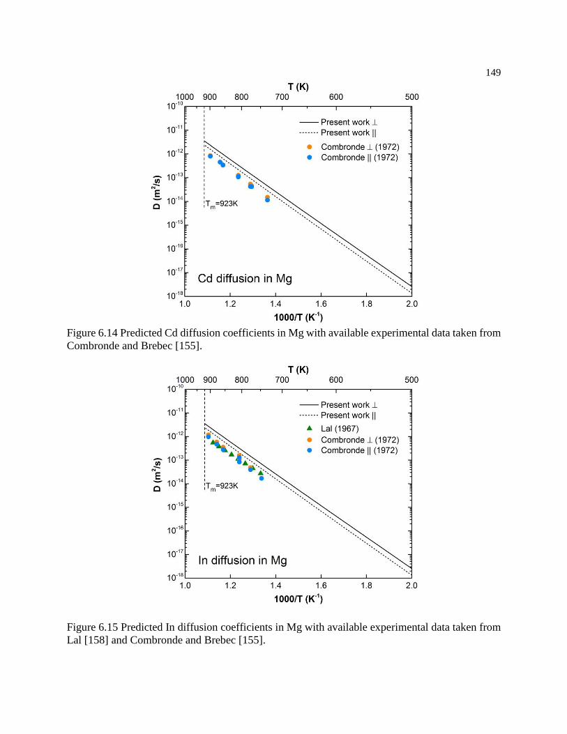
149
Figure 6.14 Predicted Cd diffusion coefficients in Mg with available experimental data taken from
Combronde and Brebec [155].
Figure 6.15 Predicted In diffusion coefficients in Mg with available experimental data taken from
Lal [158] and Combronde and Brebec [155].

150
Figure 6.16 Predicted Fe diffusion coefficients in Mg with available experimental data taken from
Pavlinov et al. [164].
Figure 6.17 Predicted Ga diffusion coefficients in Mg with available experimental data taken from
Stloukal and Čermák [165].

151
Figure 6.18 Predicted Mn diffusion coefficients in Mg with available experimental data taken from
Fujikawa [166].
Figure 6.19. Predicted Ni diffusion coefficients in Mg with available experimental data taken from
Pavlinov et al. [164].

152
Figure 6.20 Predicted Sb diffusion coefficients in Mg with available experimental data taken from
Combronde and Brebec [155].
Figure 6.21 Predicted Y diffusion coefficients in Mg with available experimental data taken from
Das et al. [167].
153
Chapter 7
First-principles predictions of dilute tracer diffusion coefficients of rare earth
elements in hcp Mg
7.1 Introduction
Rare earth (RE) elements in Mg alloys have long been known to improve the mechanical
properties of Mg alloys, especially through precipitation hardening [170,171] and refinement of
deformation texture [19]. Commercial Mg alloys containing RE elements have found wide
applications for their superior properties of creep resistance and high temperature strength, such
as WE54 and AE42. Alloying Mg with Zn/Ni/Cu with a RE can generate an important type of
strengthening phase, the long-period stacking ordered (LPSO) structures [172]. This phase can
greatly enhance the strength and ductility of Mg alloys. The diffusion of RE elements in Mg is a
critical factor determining the formation of strengthening phases such as LPSO structures.
The class of RE elements traditionally includes Sc, Y, and 15 lanthanides. The lanthanides
can be divided into two groups: the light lanthanides which contain from La to Gd, and the heavy
lanthanides which contain from Tb to Lu. It is usually very difficult experimentally to separate RE
elements due to their similar chemical nature. Therefore, REs are typically added to Mg alloys in
the form of mischmetal, which is essentially a mixture of RE elements. Recent study [173] shows
that rare earth elements do have significantly different behaviors in Mg. Therefore it is important
to understand the diffusion properties of each individual RE solutes in Mg.
In the literature, there only exist experimental diffusion coefficient measurements for La,
Ce [158], Gd, Y [167], and Nd [174]. There is a significant lack of diffusion data for RE solutes
in hcp Mg. Motivated by obtaining the accurate diffusion coefficients of RE in Mg and better

154
understanding the diffusion mechanisms of RE in Mg, first-principles calculations based on DFT
are performed in the present work to predict the diffusion coefficients of RE in Mg, including Sc,
Y and all the lanthanides (see Figure 7.1).
7.2 Diffusion theory
The diffusion equations used for the calculation of RE solutes in Mg are essentially the
same as the diffusion equations based on the 8-frequency model used for the non-RE solutes in
Chapter 6. Below is a summary of the important diffusion equations and the 8-frequency model:
Vacancy concentration adjacent to a solute atom:
expf
v
B
GC
k T
(7.1)
where 0
f f bG G G is the free energy of vacancy formation adjacent to the solute atom.
Vacancy formation free energy in pure Mg without solute:
0
1 1
1Mg Va Mgf N N
NG G G
N
(7.2)
where Va indicates a vacancy, and N the number of lattice sites in the supercell.
The solute-vacancy binding free energy:
2 1 1 1 1 1 1X Va Mg X Va Mg Mg X Mg Vab N N N NG G G G G (7.3)
where X represents a solute atom. The minus sign in front of bG in Eq. (7.3) is to keep the
binding energy consistent with the convention in the literature such that favorable solute-vacancy
binding is positive [148].
Jump frequencies of solutes
155
exp mB
B
Gk T
h k T
(7.4)
where m TS ISG G G is the solute migration free energy barrier with TSG being the free energy
of the transition state (TS) and ISG the free energy of the initial state (IS).
Correlation factors and the 8-frequency model
The correlation factors of solute diffusion in an hcp lattice can be quantitatively evaluated
using the 8-frequency model developed by Ghate [150], which is analogous to the 5-frequency
model by Le Claire [151] for fcc materials. In Ghate’s model these correlation factors depend on
8 jump frequencies illustrated in Figure 6.3 and are expressed as:
2 5.512
2 5.512 2
a cAz
a c X
f
(7.5)
21 Bx
Bx
B
Sf
(7.6)
21 Ab
Ab
Ab
Sf
(7.7)
where jump distances B and Ab correspond to the net jump distances associated with jumps
within a basal plane and between adjacent basal planes, respectively (see Figure 5.1). The average
final displacements BxS and AbS are determined by solving the following system of equations:
3
2 2 5.512
a Bx By b Ab X Ab Ab
Ab
a b c X
S S S SS
(7.8)
3
2 2 5.512
a Ab b Bx X B Bx
Bx
a b c X
S S SS
(7.9)
156
2 2 5.512
a Ab b By
By
a b c X
S SS
(7.10)
Using the frequencies of each jump in the 8-frequency model, the Eqs. (7.8)~(7.10) can be
solved and the correlation factors can be calculated using Eqs. (7.5)~(7.7).
Free energies fG and mG can be obtained from DFT calculations based on the quasi-
harmonic approximations described in Section 6.3.3 to calculate the jump frequencies X , X ,
a , b , c , a , b , c , and the vacancy concentrations. The calculated diffusion coefficients D
can be fitted into the conventional Arrhenius form:
0 expB
QD D
k T
(7.11)
where Q is the diffusion activation energy and D0 the pre-exponential factor. The activation
energy Q corresponds to the enthalpy of vacancy formation, the enthalpy of solute migration, and
part of the contribution from correlation factors; the diffusion pre-exponential factor D0
corresponds to the entropy of vacancy formation, the entropy of solute migration, the lattice
parameters, and also part of the correlation factors. It should be noted that all the diffusion plots
shown in the present work were plotted using the calculated data directly from first-principles, not
the fitted Arrhenius equation.
7.3 Computational details
First-principles calculations based on DFT were employed to calculate the free energies
needed in the diffusion equations and the 8-frequency model. The ion-electron interaction was
described by the projector augmented plane-wave (PAW) method [48] and the X-C functional was

157
described by an improved GGA of PBEsol [32], as implemented in the VASP 5.3.2 code [97]. The
suitability of PBEsol for the present study is discussed in the Section 5.4.1 and 5.4.2. An energy
cut-off of 350 eV was used for the plane-wave expansion of the electronic wave functions.
DFT has well-documented difficulties in describing the 4f electrons of the lanthanides,
especially their tendency to form localized states. In the literature, a common solution is to use the
so-called “frozen-core” potentials to treat the 4f electrons as the core electrons. This approach has
been shown to successfully reproduce the lanthanide contraction effect [175]. The frozen potentials
can also reproduce the experimentally observed Al-RE binary convex hulls [176]. These evidence
gives us the confidence that the frozen potential can predict the thermodynamic and diffusion
properties of Mg-RE alloys. In the present work we used the frozen potentials for all the
lanthanides, as shown in Figure 7.1.
We performed rigorous supercell size and k-point convergence test. After tests of supercell
size, we chose a 96-atom supercell (4×4×3 conventional hcp unit cells) for all the lanthanides,
which was sufficient to isolate the vacancy and solute atom from the periodic images. All structural
degrees of freedom (ionic coordinates, cell volume, and cell shape) in the supercell were fully
relaxed via a conjugate gradient method to an energy convergence of 10-5 eV/atom, followed by a
final static calculation using the tetrahedron method with Blöchl corrections [122] with energy
convergence of 10-6 eV/atom to get the accurate total energy. a 5×5×4 -centered k-point mesh
was used in structural relaxation and a 7×7×7 -centered k-point mesh in subsequent static
calculations. Other computational details such as the transition state search and the quasi-harmonic
approach to the free energy are the same as those used in the calculation of non-RE elements (see
Section 6.3).
158
7.4 Results and discussion
7.4.1 Solute-vacancy binding energy
The calculated solute-vacancy binding energies of RE-Va can be found in Table 7.1. Figure
7.7 shows the basal solute-vacancy binding energies as a function of the atomic number for all the
RE elements. As can be seen from Figure 7.7, the basal solute-vacancy binding energy gradually
decreases as the atomic number increases for most of the lanthanides. Yb is an exception because
it has fully filled ground state f-bands, resulting its unique electronic behavior [175]. The
decreasing trend can be understood by the strain model as discussed by Shin and Wolverton [136]
and Saal and Wolverton [147]. Solute atoms with large atomic size tend to relax toward the
vacancy to release the local strain. Therefore, the larger the solute atom, the stronger binding
between the solute and vacancy pair. Our calculated results agree well with the solute-vacancy
binding energies of RE elements in Mg calculated by Saal and Wolverton [147] using PBE as the
X-C functional.
7.4.2 Correlation effects and correlation energy
As is discussed in Section 6.4.3, when the direct solute migration barriers are significantly
smaller than the other solvent migration barriers, the solute atom tends to fast oscillate between
the two atomic sites. This leads to strong correlation effects which cannot be neglected during the
diffusion calculation. In order to quantify the correlation effects for each solute, we define the
correlation energy if
E [124] :

159
0 exp if
i i
B
Ef f
k T
(7.12)
where if is the correlation factor in the 8-frequency model. The calculated correlation factors
based on Eqs. (7.5)~(7.7) can be fitted into an Arrhenius-like equation (7.12). The exponential
term if
E is the correlation energy. It measures the contribution to the total activation energy for
an individual solute from the correlation effects.
Figure 7.12 shows the contributions to the normal activation energies Q for Mg self-
diffusion, Ca, and RE solute diffusion. The normal activation energy Q has three contributions:
vacancy formation energy with the correction of the solute-vacancy binding energy (0
f bindE E ),
solute migration energy ( XE ), and the correlation energy AzfE . From Figure 7.12 we can see that
for RE diffusion, the vacancy formation energy (~0.86 eV) is the dominant energy contribution
for the activation energy. The solute migration energy gradually increases as the atomic number
increases for the lanthanides, while the correlation energy gradually decreases as the atomic
number increases. Light REs such as La, Ce, Pr, and Nd have relatively large correlation energies
while heavy REs like Tb, Dy, Ho, Er, Tm, and Lu have diminishingly small correlation energies.
These observations are consistent with the conclusion drew in Section 6.4.3, that is smaller direct
migration barriers lead to stronger correlation effects. Yb has large correlation energy and its
unique behavior can be traced back to its fully filled f-bands.
160
7.4.3 Diffusion data
The calculated diffusion coefficients of RE elements and their Arrhenius parameters D0
and Q can be found in Table 7.3. The basal solute diffusion coefficients for all the RE elements are
plotted in Figure 7.2. Contrary to the common belief that RE elements diffuse slowly in hcp Mg
due to their large atomic size, they diffuse reasonably fast in Mg compared with transition metal
elements. Light RE elements like La, Ce, Pr, Pm, Nd, and Sm diffuse faster than Mg self-diffusion,
while heavy RE elements such as Eu, Tb, Gd, Er, Ho, Dy, Tm, and Lu tend to diffuse slower than
Mg self-diffusion. The diffusion coefficients of all the RE elements have two orders of magnitude
difference at most (La and Sc).
Comparisons between the current first-principles prediction and experimental
measurements are made and good agreements are achieved, as shown for La (Figure 7.4), Ce
(Figure 7.5), Gd (Figure 7.6). It can be seen that good agreements with experimental result can
only be achieved with the consideration of the strong correlation effects for La and Ce.
Table 7.2 shows the energy barriers of vacancy migration for various RE solutes in hcp Mg
calculated based on the 8-frequency model. The activation energies gradually increases as the
atomic number increases for the lanthanides (not including Yb), as shown in Figure 7.3. This trend
is consistent with the increasing trend of solute migration barriers as a function of atomic number
for RE elements. As the atomic number increases, the atomic size actually decreases due to the
lanthanide contraction. The solute induced volume difference XV (see Section 6.4.1) is a
quantitative measure of the atomic size for each RE element X. As the atomic size of lanthanide
elements increases, the XV also increases, while the basal solute migration barrier XE actually
decreases. As shown in Figure 7.8, a linear relationship exists between XV and XE for all the

161
lanthanides except for Yb. This again can be explained by the strain argument used in explaining
the barrier trend for non-RE elements. Large atomic size induces large local strain and this leads
to more free space for the atom to jump and thus lowers the migration barrier. Bulk modulus of
the dilute alloy Mg95X can be used as a measure of the bonding strength between the RE elements
and the Mg matrix. The stronger bonding between RE elements and the Mg matrix, the more
difficult it will be for RE atom to migrate. Figure 7.9 demonstrates that it is indeed the case with
the exception of Yb.
Small direct solute migration barriers compared with other solvent migration barriers lead
to strong correlation effects. The correlation effects are non-negligible for light REs such as La
while it is negligible for heavy REs such as Lu. Figure 7.10 and Figure 7.11 show the calculated
correlation factors and the diffusion coefficients for La and Lu with/without correlation
considered. A significant difference of correlation effects can be found for these two RE elements.
7.5 Conclusions
We performed a systematic study of dilute solute diffusion coefficients of 17 substitutional
RE alloying elements in hcp Mg. The 8-frequency model for solute diffusion within an hcp lattice
has been used to compute the correlation factors for different jumps. All the energies and
vibrational quantities required to compute the jump frequencies and hence derive the RE solute
diffusion coefficients from the 8-frequency model are calculated with the DFT based first-
principles calculations in terms of the X-C functional of PBEsol and the quasi-harmonic Debye
model. Saddle point configurations are predicted using the first-principles based CI-NEB method.
It is found that:

162
(1) The first-principles calculations based on DFT using PBEsol X-C functional with frozen
potential for REs are capable of describing the RE-Mg interactions. Reasonable values of
solute-vacancy binding energies and diffusion coefficients are predicted and agree well
with experiments.
(2) Light RE elements such as La, Ce, Pr, Pm, Nd, and Sm diffuse faster than Mg self-
diffusion, while heavy RE elements such as Eu, Tb, Gd, Er, Ho, Dy, Tm, and Lu tend to
diffuse slower than Mg self-diffusion.
(3) The correlation energies increase with solute size. They have a compensating effect on the
size effects on solute-vacancy binding energy bindE and migration energy XE alone.
(4) The calculated migration barriers of RE elements decreases in a linear fashion as the atomic
size increases, with Yb being an exception due to its fully filled f-bands.
(5) All of these size effects of RE elements can be rationalized in an elastic context, where
large solutes bind to vacancies as a means of relieving strain on the host matrix.
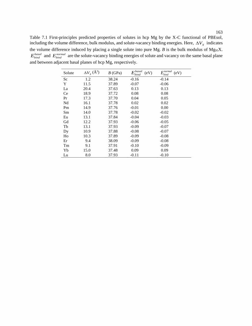
163
Table 7.1 First-principles predicted properties of solutes in hcp Mg by the X-C functional of PBEsol,
including the volume difference, bulk modulus, and solute-vacancy binding energies. Here, XV indicates
the volume difference induced by placing a single solute into pure Mg. B is the bulk modulus of Mg95X. basal
bindE and normal
bindE are the solute-vacancy binding energies of solute and vacancy on the same basal plane
and between adjacent basal planes of hcp Mg, respectively.
Solute XV (Å3) B (GPa) basal
bindE (eV) normal
bindE (eV)
Sc 1.2 38.24 -0.16 -0.14
Y 11.5 37.89 -0.07 -0.06
La 20.4 37.63 0.13 0.13
Ce 18.9 37.72 0.08 0.08
Pr 17.3 37.70 0.04 0.05
Nd 16.1 37.78 0.02 0.02
Pm 14.9 37.76 -0.01 0.00
Sm 14.0 37.78 -0.02 -0.02
Eu 13.1 37.84 -0.04 -0.03
Gd 12.2 37.93 -0.06 -0.05
Tb 13.1 37.93 -0.09 -0.07
Dy 10.9 37.88 -0.08 -0.07
Ho 10.3 37.89 -0.09 -0.08
Er 9.4 38.09 -0.09 -0.08
Tm 9.1 37.91 -0.10 -0.09
Yb 15.0 37.48 0.09 0.09
Lu 8.0 37.93 -0.11 -0.10
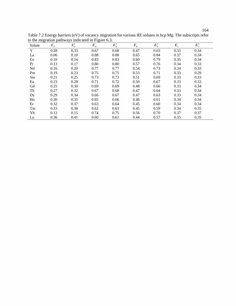
164
Table 7.2 Energy barriers (eV) of vacancy migration for various RE solutes in hcp Mg. The subscripts refer
to the migration pathways indicated in Figure 6.3.
Solute XE XE
aE aE
bE bE
cE cE
Y 0.28 0.33 0.67 0.68 0.47 0.63 0.33 0.34
La 0.06 0.10 0.88 0.88 0.65 0.84 0.37 0.34
Ce 0.10 0.14 0.83 0.83 0.60 0.79 0.35 0.34
Pr 0.13 0.17 0.80 0.80 0.57 0.76 0.34 0.33
Nd 0.16 0.20 0.77 0.77 0.54 0.73 0.34 0.33
Pm 0.19 0.23 0.75 0.75 0.53 0.71 0.33 0.29
Sm 0.21 0.25 0.73 0.73 0.51 0.69 0.33 0.33
Eu 0.23 0.28 0.71 0.72 0.50 0.67 0.33 0.33
Gd 0.25 0.30 0.69 0.69 0.48 0.66 0.33 0.34
Tb 0.27 0.32 0.67 0.68 0.47 0.64 0.33 0.34
Dy 0.29 0.34 0.66 0.67 0.47 0.63 0.33 0.34
Ho 0.30 0.35 0.65 0.66 0.46 0.61 0.34 0.34
Er 0.32 0.37 0.63 0.64 0.45 0.60 0.34 0.34
Tm 0.33 0.38 0.62 0.63 0.45 0.59 0.34 0.35
Yb 0.12 0.15 0.74 0.75 0.56 0.70 0.37 0.37
Lu 0.36 0.41 0.60 0.61 0.44 0.57 0.35 0.35
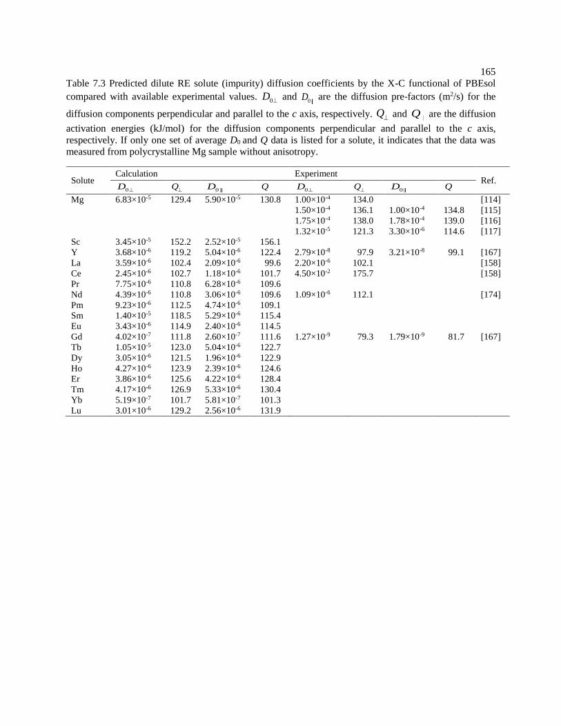
165
Table 7.3 Predicted dilute RE solute (impurity) diffusion coefficients by the X-C functional of PBEsol
compared with available experimental values. 0D and 0D are the diffusion pre-factors (m2/s) for the
diffusion components perpendicular and parallel to the c axis, respectively. Q and Q are the diffusion
activation energies (kJ/mol) for the diffusion components perpendicular and parallel to the c axis,
respectively. If only one set of average D0 and Q data is listed for a solute, it indicates that the data was
measured from polycrystalline Mg sample without anisotropy.
Solute Calculation Experiment
Ref. 0D
Q
0D Q 0D
Q
0D Q
Mg 6.83×10⁻⁵ 129.4 5.90×10⁻⁵ 130.8 1.00×10⁻⁴ 134.0 [114]
1.50×10⁻⁴ 136.1 1.00×10⁻⁴ 134.8 [115]
1.75×10⁻⁴ 138.0 1.78×10⁻⁴ 139.0 [116]
1.32×10⁻⁵ 121.3 3.30×10⁻⁶ 114.6 [117]
Sc 3.45×10⁻⁵ 152.2 2.52×10⁻⁵ 156.1
Y 3.68×10⁻⁶ 119.2 5.04×10⁻⁶ 122.4 2.79×10⁻⁸ 97.9 3.21×10⁻⁸ 99.1 [167]
La 3.59×10⁻⁶ 102.4 2.09×10⁻⁶ 99.6 2.20×10⁻⁶ 102.1 [158]
Ce 2.45×10⁻⁶ 102.7 1.18×10⁻⁶ 101.7 4.50×10⁻² 175.7 [158]
Pr 7.75×10⁻⁶ 110.8 6.28×10⁻⁶ 109.6
Nd 4.39×10⁻⁶ 110.8 3.06×10⁻⁶ 109.6 1.09×10⁻⁶ 112.1 [174]
Pm 9.23×10⁻⁶ 112.5 4.74×10⁻⁶ 109.1
Sm 1.40×10⁻⁵ 118.5 5.29×10⁻⁶ 115.4
Eu 3.43×10⁻⁶ 114.9 2.40×10⁻⁶ 114.5
Gd 4.02×10⁻⁷ 111.8 2.60×10⁻⁷ 111.6 1.27×10⁻⁹ 79.3 1.79×10⁻⁹ 81.7 [167]
Tb 1.05×10⁻⁵ 123.0 5.04×10⁻⁶ 122.7
Dy 3.05×10⁻⁶ 121.5 1.96×10⁻⁶ 122.9
Ho 4.27×10⁻⁶ 123.9 2.39×10⁻⁶ 124.6
Er 3.86×10⁻⁶ 125.6 4.22×10⁻⁶ 128.4
Tm 4.17×10⁻⁶ 126.9 5.33×10⁻⁶ 130.4
Yb 5.19×10⁻⁷ 101.7 5.81×10⁻⁷ 101.3
Lu 3.01×10⁻⁶ 129.2 2.56×10⁻⁶ 131.9
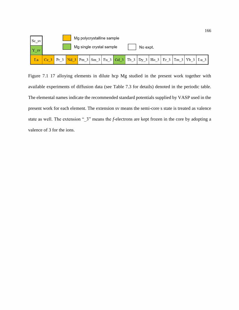
166
Figure 7.1 17 alloying elements in dilute hcp Mg studied in the present work together with
available experiments of diffusion data (see Table 7.3 for details) denoted in the periodic table.
The elemental names indicate the recommended standard potentials supplied by VASP used in the
present work for each element. The extension sv means the semi-core s state is treated as valence
state as well. The extension “_3” means the f-electrons are kept frozen in the core by adopting a
valence of 3 for the ions.

167
Figure 7.2 Calculated basal diffusion coefficients of rare earth elements form the present first-
principles calculations.

168
Figure 7.3 Calculated basal activation energy of rare earth elements in Mg

169
Figure 7.4 Calculated diffusion coefficients of La in Mg compared with experiments [158].
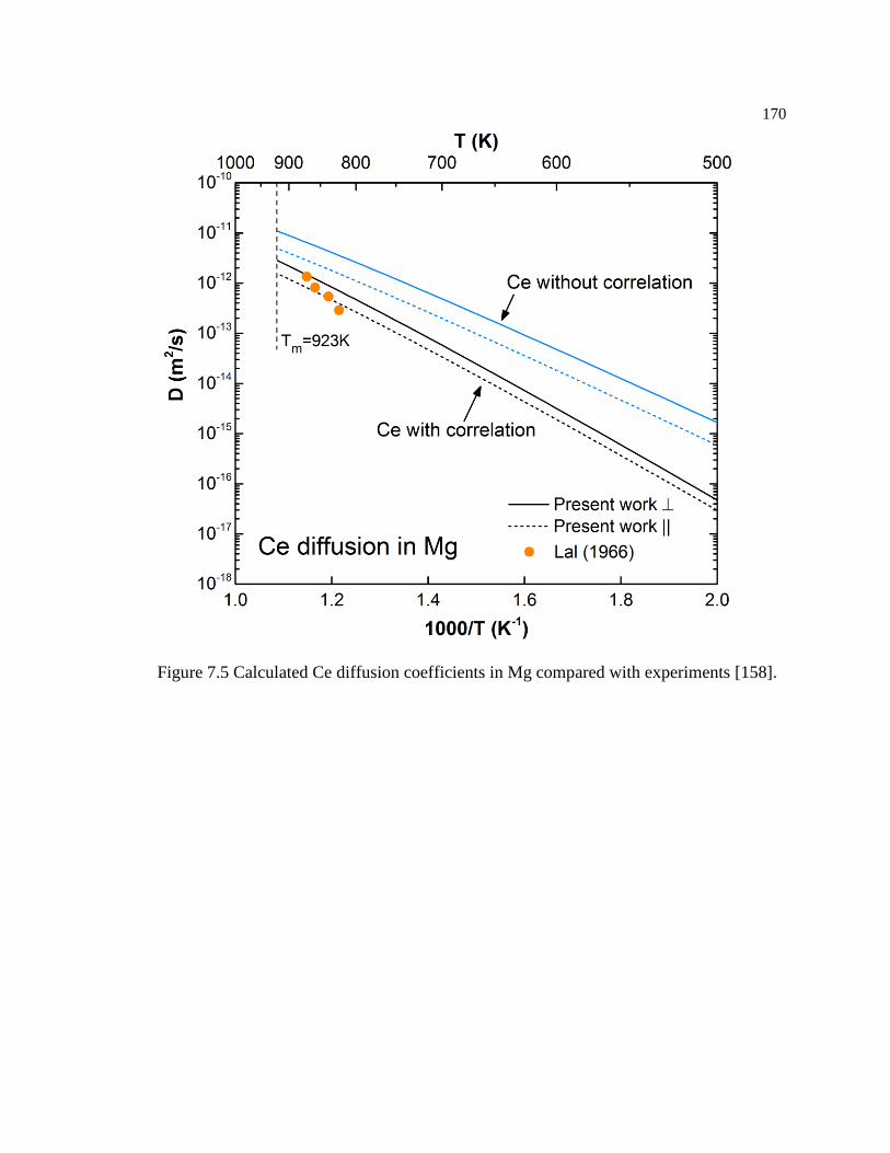
170
Figure 7.5 Calculated Ce diffusion coefficients in Mg compared with experiments [158].
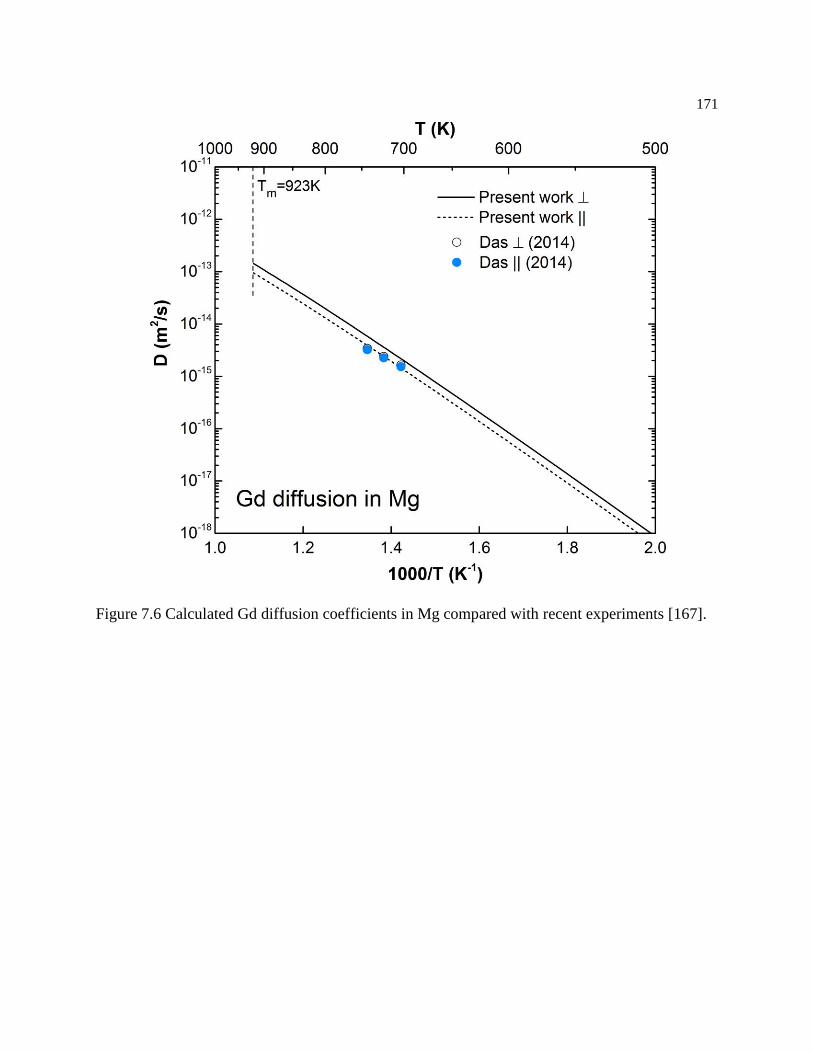
171
Figure 7.6 Calculated Gd diffusion coefficients in Mg compared with recent experiments [167].

172
Figure 7.7 Calculated basal solute-vacancy binding energy as a function of atomic number.
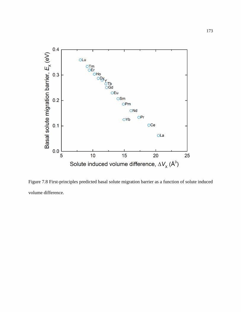
173
Figure 7.8 First-principles predicted basal solute migration barrier as a function of solute induced
volume difference.

174
Figure 7.9 Calculated diffusion cofficients at 800K as a function of predicted bulk modulus in
Mg95X supercells.
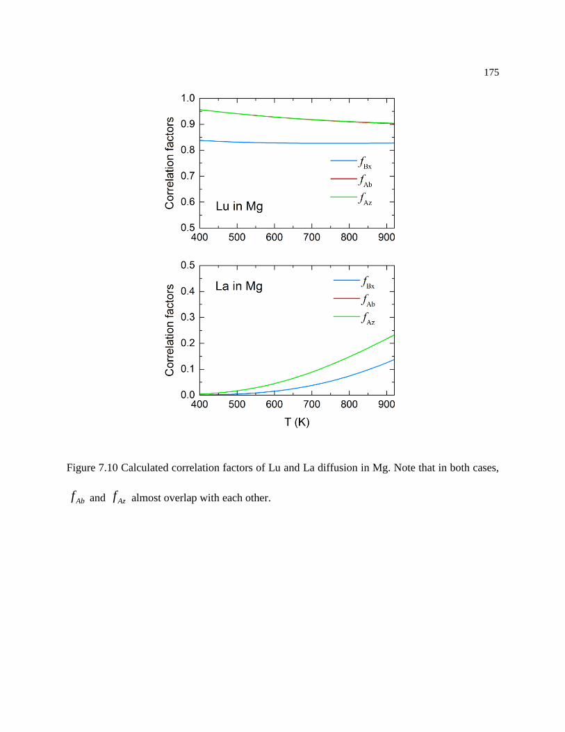
175
Figure 7.10 Calculated correlation factors of Lu and La diffusion in Mg. Note that in both cases,
Abf and Azf almost overlap with each other.
176
Figure 7.11 Calculated La and Lu diffusion coefficients in Mg with/without correlation effects
considered.
177
Figure 7.12 Contributions (vacancy formation energy, vacancy migration energy, and correlation
energy) to the normal activation energies for Mg self-diffusion, Ca, and RE solute diffusion.

178
Chapter 8
Conclusions and future work
8.1 Summary and final conclusions
As an effort for computational and data-driven development of advanced Mg-based alloys,
we present a comprehensive study of the effects of alloying elements on the thermodynamic and
diffusion properties of Mg alloys. For the thermodynamic properties, two ternary systems Mg-Sn-
Sr and Mg-Ce-Sn were modeled with the CALPHAD technique supported by the finite
temperature first-principles calculations. Excellent agreement was achieved with the available
experimental phase diagram data in the literature. The thermodynamic databases will be useful for
high-temperature Mg-Sn alloy development containing Sr and Ce as the alloying elements. For the
diffusion properties, we calculated the dilute solute diffusion coefficients of 61 substitutional
alloying elements in hcp Mg, including rare earth elements. The 8-frequency model for solute
diffusion within an hcp lattice has been used to compute the correlation factors for different jumps.
All the energies and vibrational quantities required to compute the jump frequencies and hence
derive the solute diffusion coefficients from the 8-frequency model are calculated with the DFT
based first-principles calculations in terms of the X-C functional of PBEsol and the quasi-harmonic
Debye model. Saddle point configurations are predicted using the first-principles based CI-NEB
method. It is found that:
(1) Finite temperature first-principles calculations based on the phonon and Debye model
provide robust input thermochemical data for CALPHAD modeling and avoids the
artifact of heat capacity description from the Neumann-Kopp approximation.

179
(2) Compared with LDA and GGA, PBEsol is able to well describe both vacancy formation
energies and vibrational properties, resulting in more accurate quantitative predictions
of diffusion coefficients.
(3) Correlation effects are not negligible in solutes Ca, Na, Se, Sr, Te, Y, and all the light
lanthanides in which the direct solute migration barriers are significantly smaller than
the solvent migration barriers. This indicates that the larger solute atoms can move
faster while the smaller ones move slower, with the exception of Se.
(4) The solute diffusion coefficients in hcp Mg are roughly inversely proportional to bulk
modulus, i.e. their bonding to Mg. Transition metal elements with d electrons strongly
interact with Mg and have very large diffusion activation energies, which cannot be
explained by a simple strain model based on atomic size.
(5) The predicted solute diffusion coefficients in Mg compare remarkably well with
available experiments in the literature. For most solutes basal diffusion coefficients are
bigger than the non-basal ones. The diffusion coefficient of Ag shows anomaly with
basal and non-basal diffusion coefficients showing opposite trend compared with other
alloying elements.
(6) The calculated migration barriers of RE elements decreases in a linear fashion as the
atomic size increases, with Yb being an exception due to its fully filled f-bands. All of
these size effects of RE elements can be rationalized in an elastic context, where large
solutes bind to vacancies as a means of relieving strain on the host matrix.
(7) The present work lays the foundation of diffusion data for future rational design of
novel casting and wrought Mg alloys. The calculated diffusion data can be used to
develop CALPHAD-type diffusion mobility databases for multi-component Mg alloys

180
[14]. The theoretical methodology used herein can be readily applied to solute diffusion
in other hcp systems.
8.2 Directions for future work
(1) Establish a CALPHAD-type multi-component diffusion mobility database for Mg alloys
using DICTRA [36].
(2) Kinetic Monte Carlo simulations of non-dilute diffusion coefficients of solutes in Mg
alloys.
(3) Simulations of nucleation phenomena in Mg alloys. Kinetic Monte Carlo can be used to
study how the alloy composition (microalloying additions [177]) can affect the early-
stage nucleation phenomenon and change the precipitate microstructure, like number
density of the precipitates.
(4) Phase field simulations of precipitate morphology evolution using the calculated
diffusion coefficients.

181
Appendix A
Thermo-Calc Mg-Sn-Sr database
ELEMENT /- ELECTRON_GAS 0.0000E+00 0.0000E+00 0.0000E+00!
ELEMENT VA VACUUM 0.0000E+00 0.0000E+00 0.0000E+00!
ELEMENT MG HCP_A3 2.4305E+01 4.9980E+03 3.2671E+01!
ELEMENT SN BCT_A5 1.1871E+02 6.3220E+03 5.1195E+01!
ELEMENT SR FCC_A1 8.7620E+01 0.0000E+00 0.0000E+00!
SPECIES MG2SN MG2SN1!
SPECIES SNSR2 SN1SR2!
FUNCTION GHSERMG 2.98150E+02 -8367.34+143.676*T-26.185*T*LN(T)
+4.858E-04*T**2-1.39367E-06*T**3+78950*T**(-1); 9.23000E+02 Y
-14130.2+204.716*T-34.3088*T*LN(T)+1.03819E+28*T**(-9); 3.00000E+03
N !
FUNCTION GHSERSN 1.00000E+02 -7958.517+122.765451*T-25.858*T*LN(T)
+5.1185E-04*T**2-3.192767E-06*T**3+18440*T**(-1); 2.50000E+02 Y
-5855.135+65.443315*T-15.961*T*LN(T)-.0188702*T**2+3.121167E-06*T**3
-61960*T**(-1); 5.05080E+02 Y
+2524.724+4.005269*T-8.2590486*T*LN(T)-.016814429*T**2
+2.623131E-06*T**3-1081244*T**(-1)-1.2307E+25*T**(-9); 8.00000E+02 Y
-8256.959+138.99688*T-28.4512*T*LN(T)-1.2307E+25*T**(-9); 3.00000E+03
N !
FUNCTION GHSERSR 2.98150E+02 -7532.367+107.183879*T-23.905*T*LN(T)
-.00461225*T**2-1.67477E-07*T**3-2055*T**(-1); 8.20000E+02 Y
-13380.102+153.196104*T-30.0905432*T*LN(T)-.003251266*T**2
+1.84189E-07*T**3+850134*T**(-1); 3.00000E+03 N !
FUNCTION GLIQMG 2.98150E+02 +GHSERMG+8202.24-8.83693*T
-8.0176E-20*T**7; 9.23000E+02 Y
+8690.32-9.39216*T+GHSERMG-1.03819E+28*T**(-9); 3.00000E+03 N !
FUNCTION GLIQSN 1.00000E+02 -855.425+108.677684*T-25.858*T*LN(T)
+5.1185E-04*T**2-3.192767E-06*T**3+18440*T**(-1)+1.47031E-18*T**7;
2.50000E+02 Y
+1247.957+51.355548*T-15.961*T*LN(T)-.0188702*T**2+3.121167E-06*T**3
-61960*T**(-1)+1.47031E-18*T**7; 5.05080E+02 Y
+9496.31-9.809114*T-8.2590486*T*LN(T)-.016814429*T**2
+2.623131E-06*T**3-1081244*T**(-1); 8.00000E+02 Y
-1285.372+125.182498*T-28.4512*T*LN(T); 3.00000E+03 N !
FUNCTION GLIQSR 2.98150E+02 +2194.997-10.118994*T-5.0668978*T*LN(T)
182
-.031840595*T**2+4.981237E-06*T**3-265559*T**(-1); 1.05000E+03 Y
-10855.29+213.406219*T-39.463*T*LN(T); 3.00000E+03 N !
FUNCTION UN_ASS 2.98150E+02 0.0 ; 3.00000E+02 N !
TYPE_DEFINITION % SEQ *!
DEFINE_SYSTEM_DEFAULT ELEMENT 2 !
DEFAULT_COMMAND DEF_SYS_ELEMENT VA /- !
TYPE_DEFINITION & GES A_P_D BCC_A2 MAGNETIC -1.0 4.00000E-01 !
PHASE BCC_A2 %& 2 1 3 !
CONSTITUENT BCC_A2 :MG,SN,SR : VA : !
PARAMETER G(BCC_A2,MG:VA;0) 2.98150E+02 +3100-2.1*T+GHSERMG;
3.00000E+03 N !
PARAMETER G(BCC_A2,SN:VA;0) 1.00000E+02 -3558.517+116.765451*T
-25.858*T*LN(T)+5.1185E-04*T**2-3.192767E-06*T**3+18440*T**(-1);
2.50000E+02 Y
-1455.135+59.443315*T-15.961*T*LN(T)-.0188702*T**2+3.121167E-06*T**3
-61960*T**(-1); 5.05080E+02 Y
+6924.724-1.994731*T-8.2590486*T*LN(T)-.016814429*T**2+2.623131E-06*T**3
-1081244*T**(-1)-1.2307E+25*T**(-9); 8.00000E+02 Y
-3856.959+132.99688*T-28.4512*T*LN(T)-1.2307E+25*T**(-9); 3.00000E+03 N !
PARAMETER G(BCC_A2,SR:VA;0) 2.98150E+02 -6779.234+116.583654*T
-25.6708365*T*LN(T)-.003126762*T**2+2.2965E-07*T**3+27649*T**(-1);
8.20000E+02 Y
-6970.594+122.067301*T-26.57*T*LN(T)-.0019493*T**2-1.7895E-08*T**3
+16495*T**(-1); 1.05000E+03 Y
+8168.357+.423037*T-9.7788593*T*LN(T)-.009539908*T**2+5.20221E-07*T**3
-2414794*T**(-1); 3.00000E+03 N !
PARAMETER G(BCC_A2,MG,SR:VA;0) 2.98140E+02 20000; 3.00000E+03 N !
PARAMETER G(BCC_A2,SN,SR:VA;0) 2.98140E+02 50000; 3.00000E+03 N !
PHASE BCT_A5 % 1 1.0 !
CONSTITUENT BCT_A5 :SN,SR : !
PARAMETER G(BCT_A5,SN;0) 1.00000E+02 +GHSERSN; 3.00000E+03 N !
PARAMETER G(BCT_A5,SR;0) 2.98150E+02 +GHSERSR+25000; 3.00000E+03 N
!
PARAMETER G(BCT_A5,SN,SR;0) 2.98150E+02 -63355.1281; 3.00000E+03 N !
PARAMETER G(BCT_A5,SN,SR;1) 2.98150E+02 -59395.4326; 3.00000E+03 N !
TYPE_DEFINITION ' GES A_P_D CBCC_A12 MAGNETIC -3.0 2.80000E-01 !
PHASE CBCC_A12 %' 2 1 1 !
183
CONSTITUENT CBCC_A12 :MG,SN : VA : !
PARAMETER G(CBCC_A12,MG:VA;0) 2.98150E+02 +4602.4-
3.011*T+GHSERMG;
3.00000E+03 N !
PARAMETER G(CBCC_A12,SN:VA;0) 1.00000E+02 -5958.517+122.765451*T
-25.858*T*LN(T)+5.1185E-04*T**2-3.192767E-06*T**3+18440*T**(-1);
2.50000E+02 Y
-3855.135+65.443315*T-15.961*T*LN(T)-.0188702*T**2+3.121167E-06*T**3
-61960*T**(-1); 5.05080E+02 Y
+4524.724+4.005269*T-8.2590486*T*LN(T)-.016814429*T**2+2.623131E-06*T**3
-1081244*T**(-1)-1.2307E+25*T**(-9); 8.00000E+02 Y
-6256.959+138.99688*T-28.4512*T*LN(T)-1.2307E+25*T**(-9); 3.00000E+03 N !
PHASE CUB_A13 % 2 1 1 !
CONSTITUENT CUB_A13 :MG,SN : VA : !
PARAMETER G(CUB_A13,MG:VA;0) 2.98150E+02 +5000-3*T+GHSERMG;
3.00000E+03 N !
PARAMETER G(CUB_A13,SN:VA;0) 1.00000E+02 -5958.517+122.765451*T
-25.858*T*LN(T)+5.1185E-04*T**2-3.192767E-06*T**3+18440*T**(-1);
2.50000E+02 Y
-3855.135+65.443315*T-15.961*T*LN(T)-.0188702*T**2+3.121167E-06*T**3
-61960*T**(-1); 5.05080E+02 Y
+4524.724+4.005269*T-8.2590486*T*LN(T)-.016814429*T**2+2.623131E-06*T**3
-1081244*T**(-1)-1.2307E+25*T**(-9); 8.00000E+02 Y
-6256.959+138.99688*T-28.4512*T*LN(T)-1.2307E+25*T**(-9); 3.00000E+03 N !
PHASE DIAMOND_A4 % 1 1.0 !
CONSTITUENT DIAMOND_A4 :SN : !
PARAMETER G(DIAMOND_A4,SN;0) 1.00000E+02 -9579.608+114.007785*T
-22.972*T*LN(T)-.00813975*T**2+2.7288E-06*T**3+25615*T**(-1); 2.98150E+02
Y
-9063.001+104.84654*T-21.5750771*T*LN(T)-.008575282*T**2
+1.784447E-06*T**3-2544*T**(-1); 8.00000E+02 Y
-10909.351+147.396535*T-28.4512*T*LN(T); 3.00000E+03 N !
TYPE_DEFINITION ( GES A_P_D FCC_A1 MAGNETIC -3.0 2.80000E-01 !
PHASE FCC_A1 %( 2 1 1 !
CONSTITUENT FCC_A1 :MG,SN,SR : VA : !

184
PARAMETER G(FCC_A1,MG:VA;0) 2.98150E+02 +2600-.9*T+GHSERMG;
3.00000E+03 N !
PARAMETER G(FCC_A1,SN:VA;0) 2.98150E+02 -345.135+56.983315*T
-15.961*T*LN(T)-.0188702*T**2+3.121167E-06*T**3-61960*T**(-1);
5.05080E+02 Y
+8034.724-4.454731*T-8.2590486*T*LN(T)-.016814429*T**2+2.623131E-06*T**3
-1081244*T**(-1)-1.2307E+25*T**(-9); 8.00000E+02 Y
-2746.959+130.53688*T-28.4512*T*LN(T)-1.2307E+25*T**(-9); 3.00000E+03 N !
PARAMETER G(FCC_A1,SR:VA;0) 2.98150E+02 +GHSERSR; 3.00000E+03 N !
PARAMETER G(FCC_A1,MG,SR:VA;0) 2.98140E+02 20000; 3.00000E+03 N !
PARAMETER G(FCC_A1,SN,SR:VA;0) 2.98150E+02 -43803.4972; 3.00000E+03
N !
PARAMETER G(FCC_A1,SN,SR:VA;1) 2.98150E+02 41065.8786; 3.00000E+03 N
!
TYPE_DEFINITION ) GES A_P_D HCP_A3 MAGNETIC -3.0 2.80000E-01 !
PHASE HCP_A3 %) 2 1 .5 !
CONSTITUENT HCP_A3 :MG,SN,SR : VA : !
PARAMETER G(HCP_A3,MG:VA;0) 2.98150E+02 +GHSERMG; 3.00000E+03 N
!
PARAMETER G(HCP_A3,SN:VA;0) 2.98150E+02 -1955.135+57.797315*T
-15.961*T*LN(T)-.0188702*T**2+3.121167E-06*T**3-61960*T**(-1);
5.05080E+02 Y
+6424.724-3.640731*T-8.2590486*T*LN(T)-.016814429*T**2+2.623131E-06*T**3
-1081244*T**(-1)-1.2307E+25*T**(-9); 8.00000E+02 Y
-4356.959+131.35088*T-28.4512*T*LN(T)-1.2307E+25*T**(-9); 3.00000E+03 N
!
PARAMETER G(HCP_A3,SR:VA;0) 2.98150E+02 -7282.367+107.883879*T
-23.905*T*LN(T)-.00461225*T**2-1.67477E-07*T**3-2055*T**(-1); 8.20000E+02
Y
-13130.102+153.896104*T-30.0905432*T*LN(T)-.003251266*T**2
+1.84189E-07*T**3+850134*T**(-1); 3.00000E+03 N !
PARAMETER G(HCP_A3,MG,SN:VA;0) 2.98150E+02 -30000-3*T; 3.00000E+03
N !
PARAMETER G(HCP_A3,MG,SN:VA;1) 2.98150E+02
-11293.8-4.42051*T; 3.00000E+03 N !
PARAMETER G(HCP_A3,MG,SR:VA;0) 2.98150E+02 10000; 3.00000E+03 N !
PARAMETER G(HCP_A3,SN,SR:VA;0) 2.98150E+02 50000; 3.00000E+03 N !
PHASE LAVES_C14 % 2 2 1 !
CONSTITUENT LAVES_C14 :MG,SR : MG,SR : !
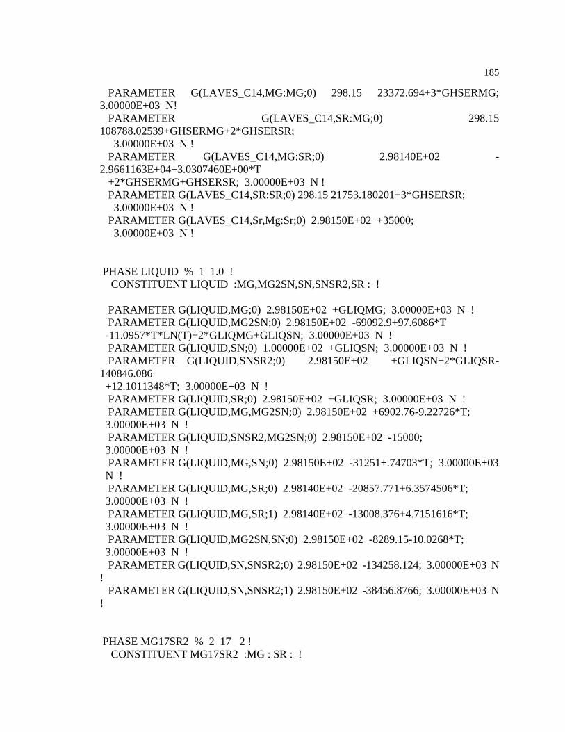
185
PARAMETER G(LAVES_C14,MG:MG;0) 298.15 23372.694+3*GHSERMG;
3.00000E+03 N!
PARAMETER G(LAVES_C14,SR:MG;0) 298.15
108788.02539+GHSERMG+2*GHSERSR;
3.00000E+03 N !
PARAMETER G(LAVES_C14,MG:SR;0) 2.98140E+02 -
2.9661163E+04+3.0307460E+00*T
+2*GHSERMG+GHSERSR; 3.00000E+03 N !
PARAMETER G(LAVES_C14,SR:SR;0) 298.15 21753.180201+3*GHSERSR;
3.00000E+03 N !
PARAMETER G(LAVES_C14,Sr,Mg:Sr;0) 2.98150E+02 +35000;
3.00000E+03 N !
PHASE LIQUID % 1 1.0 !
CONSTITUENT LIQUID :MG,MG2SN,SN,SNSR2,SR : !
PARAMETER G(LIQUID,MG;0) 2.98150E+02 +GLIQMG; 3.00000E+03 N !
PARAMETER G(LIQUID,MG2SN;0) 2.98150E+02 -69092.9+97.6086*T
-11.0957*T*LN(T)+2*GLIQMG+GLIQSN; 3.00000E+03 N !
PARAMETER G(LIQUID,SN;0) 1.00000E+02 +GLIQSN; 3.00000E+03 N !
PARAMETER G(LIQUID,SNSR2;0) 2.98150E+02 +GLIQSN+2*GLIQSR-
140846.086
+12.1011348*T; 3.00000E+03 N !
PARAMETER G(LIQUID,SR;0) 2.98150E+02 +GLIQSR; 3.00000E+03 N !
PARAMETER G(LIQUID,MG,MG2SN;0) 2.98150E+02 +6902.76-9.22726*T;
3.00000E+03 N !
PARAMETER G(LIQUID,SNSR2,MG2SN;0) 2.98150E+02 -15000;
3.00000E+03 N !
PARAMETER G(LIQUID,MG,SN;0) 2.98150E+02 -31251+.74703*T; 3.00000E+03
N !
PARAMETER G(LIQUID,MG,SR;0) 2.98140E+02 -20857.771+6.3574506*T;
3.00000E+03 N !
PARAMETER G(LIQUID,MG,SR;1) 2.98140E+02 -13008.376+4.7151616*T;
3.00000E+03 N !
PARAMETER G(LIQUID,MG2SN,SN;0) 2.98150E+02 -8289.15-10.0268*T;
3.00000E+03 N !
PARAMETER G(LIQUID,SN,SNSR2;0) 2.98150E+02 -134258.124; 3.00000E+03 N
!
PARAMETER G(LIQUID,SN,SNSR2;1) 2.98150E+02 -38456.8766; 3.00000E+03 N
!
PHASE MG17SR2 % 2 17 2 !
CONSTITUENT MG17SR2 :MG : SR : !
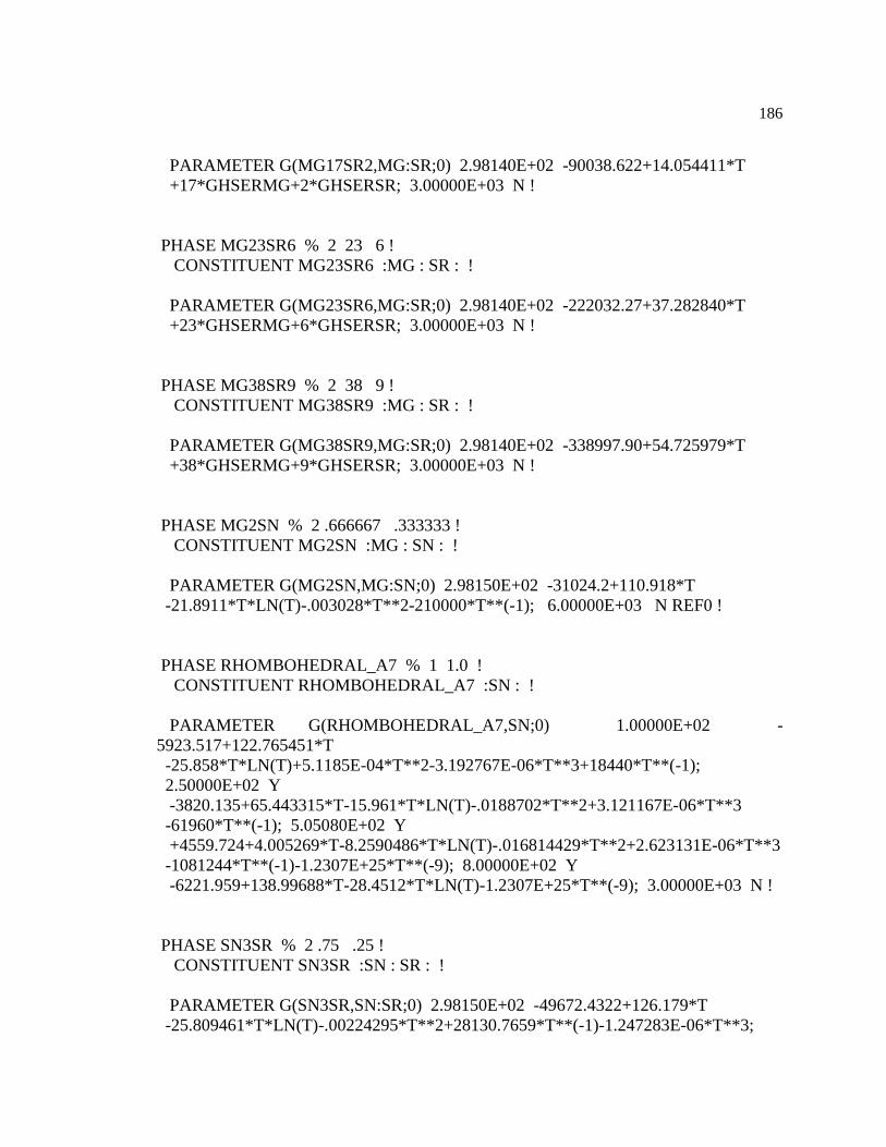
186
PARAMETER G(MG17SR2,MG:SR;0) 2.98140E+02 -90038.622+14.054411*T
+17*GHSERMG+2*GHSERSR; 3.00000E+03 N !
PHASE MG23SR6 % 2 23 6 !
CONSTITUENT MG23SR6 :MG : SR : !
PARAMETER G(MG23SR6,MG:SR;0) 2.98140E+02 -222032.27+37.282840*T
+23*GHSERMG+6*GHSERSR; 3.00000E+03 N !
PHASE MG38SR9 % 2 38 9 !
CONSTITUENT MG38SR9 :MG : SR : !
PARAMETER G(MG38SR9,MG:SR;0) 2.98140E+02 -338997.90+54.725979*T
+38*GHSERMG+9*GHSERSR; 3.00000E+03 N !
PHASE MG2SN % 2 .666667 .333333 !
CONSTITUENT MG2SN :MG : SN : !
PARAMETER G(MG2SN,MG:SN;0) 2.98150E+02 -31024.2+110.918*T
-21.8911*T*LN(T)-.003028*T**2-210000*T**(-1); 6.00000E+03 N REF0 !
PHASE RHOMBOHEDRAL_A7 % 1 1.0 !
CONSTITUENT RHOMBOHEDRAL_A7 :SN : !
PARAMETER G(RHOMBOHEDRAL_A7,SN;0) 1.00000E+02 -
5923.517+122.765451*T
-25.858*T*LN(T)+5.1185E-04*T**2-3.192767E-06*T**3+18440*T**(-1);
2.50000E+02 Y
-3820.135+65.443315*T-15.961*T*LN(T)-.0188702*T**2+3.121167E-06*T**3
-61960*T**(-1); 5.05080E+02 Y
+4559.724+4.005269*T-8.2590486*T*LN(T)-.016814429*T**2+2.623131E-06*T**3
-1081244*T**(-1)-1.2307E+25*T**(-9); 8.00000E+02 Y
-6221.959+138.99688*T-28.4512*T*LN(T)-1.2307E+25*T**(-9); 3.00000E+03 N !
PHASE SN3SR % 2 .75 .25 !
CONSTITUENT SN3SR :SN : SR : !
PARAMETER G(SN3SR,SN:SR;0) 2.98150E+02 -49672.4322+126.179*T
-25.809461*T*LN(T)-.00224295*T**2+28130.7659*T**(-1)-1.247283E-06*T**3;
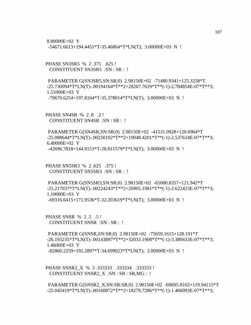
187
8.80000E+02 Y
-54671.6613+194.4451*T-35.46864*T*LN(T); 3.00000E+03 N !
PHASE SN3SR5 % 2 .375 .625 !
CONSTITUENT SN3SR5 :SN : SR : !
PARAMETER G(SN3SR5,SN:SR;0) 2.98150E+02 -71480.9341+125.3258*T
-25.730094*T*LN(T)-.00194164*T**2+28267.7619*T**(-1)-2.784854E-07*T**3;
1.51000E+03 Y
-79670.6254+197.8164*T-35.378014*T*LN(T); 3.00000E+03 N !
PHASE SN4SR % 2 .8 .2 !
CONSTITUENT SN4SR :SN : SR : !
PARAMETER G(SN4SR,SN:SR;0) 2.98150E+02 -41531.0928+120.6964*T
-25.088644*T*LN(T)-.00250102*T**2+19048.4201*T**(-1)-2.537614E-07*T**3;
6.40000E+02 Y
-42696.7818+144.9153*T-28.811579*T*LN(T); 3.00000E+03 N !
PHASE SN5SR3 % 2 .625 .375 !
CONSTITUENT SN5SR3 :SN : SR : !
PARAMETER G(SN5SR3,SN:SR;0) 2.98150E+02 -65080.8357+121.942*T
-25.217037*T*LN(T)-.00224243*T**2+20905.1981*T**(-1)-2.622423E-07*T**3;
1.10000E+03 Y
-69316.6415+171.9536*T-32.203619*T*LN(T); 3.00000E+03 N !
PHASE SNSR % 2 .5 .5 !
CONSTITUENT SNSR :SN : SR : !
PARAMETER G(SNSR,SN:SR;0) 2.98150E+02 -75659.1615+128.191*T
-26.193235*T*LN(T)-.00143897*T**2+32033.1908*T**(-1)-3.389433E-07*T**3;
1.46000E+03 Y
-82860.2259+192.2897*T-34.699023*T*LN(T); 3.00000E+03 N !
PHASE SNSR2_X % 3 .333333 .333334 .333333 !
CONSTITUENT SNSR2_X :SN : SR : SR,MG : !
PARAMETER G(SNSR2_X,SN:SR:SR;0) 2.98150E+02 -69695.8102+119.94115*T
-25.045419*T*LN(T)-.00160872*T**2+18279.7286*T**(-1)-1.466093E-07*T**3;

188
1.62000E+03 Y
-76381.9295+176.635*T-32.562229*T*LN(T); 3.00000E+03 N !
PARAMETER G(SNSR2_X,SN:SR:MG;0) 2.98150E+02 -64706.51+134.8944*T
-25.764278*T*LN(T)-8.47782E-04*T**2+54201.7448*T**(-1)-4.8882299E-07*T**3;
3.00000E+03 N !
PHASE TETRAGONAL_A6 % 1 1.0 !
CONSTITUENT TETRAGONAL_A6 :SN : !
PARAMETER G(TETRAGONAL_A6,SN;0) 2.98150E+02 -468.135+57.181195*T
-15.961*T*LN(T)-.0188702*T**2+3.121167E-06*T**3-61960*T**(-1);
5.05080E+02 Y
+7911.724-4.256851*T-8.2590486*T*LN(T)-.016814429*T**2+2.623131E-06*T**3
-1081244*T**(-1)-1.2307E+25*T**(-9); 8.00000E+02 Y
-2869.959+130.73476*T-28.4512*T*LN(T)-1.2307E+25*T**(-9); 3.00000E+03 N !
LIST_OF_REFERENCES
NUMBER SOURCE
!
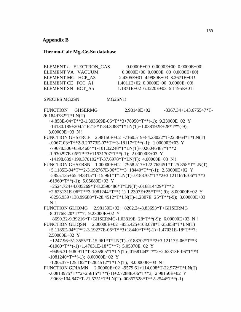
189
Appendix B
Thermo-Calc Mg-Ce-Sn database
ELEMENT /- ELECTRON_GAS 0.0000E+00 0.0000E+00 0.0000E+00!
ELEMENT VA VACUUM 0.0000E+00 0.0000E+00 0.0000E+00!
ELEMENT MG HCP_A3 2.4305E+01 4.9980E+03 3.2671E+01!
ELEMENT CE FCC_A1 1.4011E+02 0.0000E+00 0.0000E+00!
ELEMENT SN BCT_A5 1.1871E+02 6.3220E+03 5.1195E+01!
SPECIES MG2SN MG2SN1!
FUNCTION GHSERMG 2.98140E+02 -8367.34+143.675547*T-
26.1849782*T*LN(T)
+4.858E-04*T**2-1.393669E-06*T**3+78950*T**(-1); 9.23000E+02 Y
-14130.185+204.716215*T-34.3088*T*LN(T)+1.038192E+28*T**(-9);
3.00000E+03 N !
FUNCTION GHSERCE 2.98150E+02 -7160.519+84.23022*T-22.3664*T*LN(T)
-.0067103*T**2-3.20773E-07*T**3-18117*T**(-1); 1.00000E+03 Y
-79678.506+659.4604*T-101.32248*T*LN(T)+.026046487*T**2
-1.930297E-06*T**3+11531707*T**(-1); 2.00000E+03 Y
-14198.639+190.370192*T-37.6978*T*LN(T); 4.00000E+03 N !
FUNCTION GHSERSN 1.00000E+02 -7958.517+122.765451*T-25.858*T*LN(T)
+5.1185E-04*T**2-3.192767E-06*T**3+18440*T**(-1); 2.50000E+02 Y
-5855.135+65.443315*T-15.961*T*LN(T)-.0188702*T**2+3.121167E-06*T**3
-61960*T**(-1); 5.05080E+02 Y
+2524.724+4.005269*T-8.2590486*T*LN(T)-.016814429*T**2
+2.623131E-06*T**3-1081244*T**(-1)-1.2307E+25*T**(-9); 8.00000E+02 Y
-8256.959+138.99688*T-28.4512*T*LN(T)-1.2307E+25*T**(-9); 3.00000E+03
N !
FUNCTION GLIQMG 2.98150E+02 +8202.24-8.83693*T+GHSERMG
-8.0176E-20*T**7; 9.23000E+02 Y
+8690.32-9.39216*T+GHSERMG-1.03819E+28*T**(-9); 6.00000E+03 N !
FUNCTION GLIQSN 2.00000E+02 -855.425+108.678*T-25.858*T*LN(T)
+5.1185E-04*T**2-3.19277E-06*T**3+18440*T**(-1)+1.47031E-18*T**7;
2.50000E+02 Y
+1247.96+51.3555*T-15.961*T*LN(T)-.0188702*T**2+3.12117E-06*T**3
-61960*T**(-1)+1.47031E-18*T**7; 5.05070E+02 Y
+9496.31-9.80911*T-8.25905*T*LN(T)-.0168144*T**2+2.62313E-06*T**3
-1081240*T**(-1); 8.00000E+02 Y
-1285.37+125.182*T-28.4512*T*LN(T); 3.00000E+03 N !
FUNCTION GDIAMN 2.00000E+02 -9579.61+114.008*T-22.972*T*LN(T)
-.00813975*T**2+25615*T**(-1)+2.7288E-06*T**3; 2.98150E+02 Y
-9063+104.847*T-21.5751*T*LN(T)-.00857528*T**2-2544*T**(-1)
190
+1.78444E-06*T**3; 8.00000E+02 Y
-10909.4+147.397*T-28.4512*T*LN(T); 3.00000E+03 N !
FUNCTION UN_ASS 2.98150E+02 0.0 ; 3.00000E+02 N !
TYPE_DEFINITION % SEQ *!
DEFINE_SYSTEM_DEFAULT ELEMENT 2 !
DEFAULT_COMMAND DEF_SYS_ELEMENT VA /- !
PHASE LIQUID:L % 1 1.0 !
CONSTITUENT LIQUID:L : MG,CE,SN,MG2SN : !
PARAMETER G(LIQUID,MG;0) 2.98140E+02 +8202.243-8.83693*T+GHSERMG
-8.0176E-20*T**7; 9.23000E+02 Y
-5439.869+195.324057*T-34.3088*T*LN(T); 3.00000E+03 N REF0 !
PARAMETER G(LIQUID,CE;0) 2.98150E+02 +4117.865-11.423898*T
-7.5383948*T*LN(T)-.02936407*T**2+4.827734E-06*T**3-198834*T**(-1);
1.00000E+03 Y
-6730.605+183.023193*T-37.6978*T*LN(T); 4.00000E+03 N REF0 !
PARAMETER G(LIQUID,SN;0) 1.00000E+02 -855.425+108.677684*T
-25.858*T*LN(T)+5.1185E-04*T**2-3.192767E-06*T**3+18440*T**(-1)
+1.47031E-18*T**7; 2.50000E+02 Y
+1247.957+51.355548*T-15.961*T*LN(T)-.0188702*T**2+3.121167E-06*T**3
-61960*T**(-1)+1.47031E-18*T**7; 5.05080E+02 Y
+9496.31-9.809114*T-8.2590486*T*LN(T)-.016814429*T**2+2.623131E-06*T**3
-1081244*T**(-1); 8.00000E+02 Y
-1285.372+125.182498*T-28.4512*T*LN(T); 3.00000E+03 N REF0 !
PARAMETER G(LIQUID,MG2SN;0) 2.98150E+02 -69092.9+97.6086*T
-11.0957*T*LN(T)+2*GLIQMG+GLIQSN; 3.00000E+03 N REF0 !
PARAMETER G(LIQUID,CE,SN;0) 2.98150E+02 -1.8030394E+05-
1.5771700E+01*T;
6.00000E+03 N REF0 !
PARAMETER G(LIQUID,CE,SN;1) 2.98150E+02 -
1.3801121E+04+3.7889833E+01*T;
6.00000E+03 N REF0 !
PARAMETER G(LIQUID,CE,SN;2) 2.98150E+02 +3.4036953E+04; 6.00000E+03
N
REF0 !
PARAMETER G(LIQUID,CE,MG;0) 2.98150E+02 -36703.381+13.831225*T;
6.00000E+03 N REF0 !
PARAMETER G(LIQUID,CE,MG;1) 2.98150E+02 +30962.108-17.297005*T;
6.00000E+03 N REF0 !
PARAMETER G(LIQUID,CE,MG;2) 2.98150E+02 -15089.803; 6.00000E+03 N
REF0 !
PARAMETER G(LIQUID,MG,MG2SN;0) 2.98150E+02 +6902.76-9.22726*T;

191
3.00000E+03 N REF0 !
PARAMETER G(LIQUID,MG,SN;0) 2.98150E+02 -31251+.74703*T; 3.00000E+03
N REF0 !
PARAMETER G(LIQUID,MG2SN,SN;0) 2.98150E+02 -8289.15-10.0268*T;
3.00000E+03 N REF0 !
TYPE_DEFINITION & GES A_P_D BCC_A2 MAGNETIC -1.0 4.00000E-01 !
PHASE BCC_A2 %& 2 1 3 !
CONSTITUENT BCC_A2 : MG,CE,SN : VA : !
PARAMETER G(BCC_A2,CE:VA;0) 2.98150E+02 -1354.69-5.21501*T
-7.7305867*T*LN(T)-.029098402*T**2+4.784299E-06*T**3-196303*T**(-1);
1.00000E+03 Y
-12101.106+187.449688*T-37.6142*T*LN(T); 1.07200E+03 Y
-11950.375+186.333811*T-37.4627992*T*LN(T)-5.7145E-05*T**2+2.348E-
09*T**3
-25897*T**(-1); 4.00000E+03 N REF0 !
PARAMETER G(BCC_A2,SN:VA;0) 1.00000E+02 -3558.517+116.765451*T
-25.858*T*LN(T)+5.1185E-04*T**2-3.192767E-06*T**3+18440*T**(-1);
2.50000E+02 Y
-1455.135+59.443315*T-15.961*T*LN(T)-.0188702*T**2+3.121167E-06*T**3
-61960*T**(-1); 5.05080E+02 Y
+6924.724-1.994731*T-8.2590486*T*LN(T)-.016814429*T**2+2.623131E-06*T**3
-1081244*T**(-1)-1.2307E+25*T**(-9); 8.00000E+02 Y
-3856.959+132.99688*T-28.4512*T*LN(T)-1.2307E+25*T**(-9); 3.00000E+03 N
REF0 !
PARAMETER G(BCC_A2,MG:VA;0) 2.98140E+02 +3100-2.1*T+GHSERMG;
3.00000E+03 N REF0 !
PARAMETER G(BCC_A2,CE,SN:VA;0) 2.98150E+02 -1.3500000E+05;
6.00000E+03
N REF0 !
PARAMETER G(BCC_A2,CE,MG:VA;0) 2.98150E+02 -27284.091+3.6406161*T;
6.00000E+03 N REF0 !
PARAMETER G(BCC_A2,CE,MG:VA;1) 2.98150E+02 +25374.042-11.872411*T;
6.00000E+03 N REF0 !
PARAMETER G(BCC_A2,CE,MG:VA;2) 2.98150E+02 -15094.33; 6.00000E+03 N
REF0 !
PHASE BCT_A5 % 1 1.0 !
CONSTITUENT BCT_A5 :SN : !
PARAMETER G(BCT_A5,SN;0) 1.00000E+02 +GHSERSN; 3.00000E+03 N REF0
!
192
PHASE CE11SN10 % 2 11 10 !
CONSTITUENT CE11SN10 :CE : SN : !
PARAMETER G(CE11SN10,CE:SN;0) 2.98150E+02 -
1.9160000E+06+2.9455890E+03*T
-5.8734539E+02*T*LN(T)-4.7347785E-02*T**2+1.7529922E+06*T**(-1)
-3.8613666E-05*T**3; 1.64800E+03 N REF0 !
PHASE CE2SN5 % 2 2 5 !
CONSTITUENT CE2SN5 :CE : SN : !
PARAMETER G(CE2SN5,CE:SN;0) 2.98150E+02 -
4.9394939E+05+7.3814760E+02*T
-1.6486107E+02*T*LN(T)-2.8884497E-02*T**2-1.2053700E+05*T**(-1)
-2.8713284E-06*T**3; 1.41800E+03 N REF0 !
PHASE CE3SN % 2 3 1 !
CONSTITUENT CE3SN :CE : SN : !
PARAMETER G(CE3SN,CE:SN;0) 2.98150E+02 -
2.2182424E+05+2.9102475E+02*T
-7.2968254E+01*T*LN(T)-6.1236401E-02*T**2-4.4895679E+05*T**(-1)
+3.3657012E-06*T**3; 1.21300E+03 N REF0 !
PHASE CE3SN5 % 2 3 5 !
CONSTITUENT CE3SN5 :CE : SN : !
PARAMETER G(CE3SN5,CE:SN;0) 2.98150E+02 -
6.2516251E+05+7.8057805E+02*T
-1.7437377E+02*T*LN(T)-6.8228719E-02*T**2-1.8773506E+05*T**(-1)
+9.3457005E-07*T**3; 1.45300E+03 N REF0 !
PHASE CE3SN7 % 2 3 7 !
CONSTITUENT CE3SN7 :CE : SN : !
PARAMETER G(CE3SN7,CE:SN;0) 2.98150E+02 -
7.3590000E+05+1.0802160E+03*T
-2.3446599E+02*T*LN(T)-5.1437966E-02*T**2-7.4239139E+04*T**(-1)
-8.3901400E-06*T**3; 1.40800E+03 N REF0 !

193
PHASE CE5SN3 % 2 5 3 !
CONSTITUENT CE5SN3 :CE : SN : !
PARAMETER G(CE5SN3,CE:SN;0) 2.98150E+02 -
6.8176817E+05+1.4977086E+03*T
-2.8411327E+02*T*LN(T)+4.4820680E-02*T**2+1.8333661E+06*T**(-1)
-3.0400698E-05*T**3; 1.77800E+03 N REF0 !
PHASE CE5SN4 % 2 5 4 !
CONSTITUENT CE5SN4 :CE : SN : !
PARAMETER G(CE5SN4,CE:SN;0) 2.98150E+02 -
8.4500000E+05+1.3342668E+03*T
-2.6069763E+02*T*LN(T)-1.1777151E-02*T**2+9.0775311E+05*T**(-1)
-1.9600608E-05*T**3; 1.78800E+03 N REF0 !
PHASE CESN3 % 2 1 3 !
CONSTITUENT CESN3 :CE : SN : !
PARAMETER G(CESN3,CE:SN;0) 2.98150E+02 -
2.6300000E+05+4.5909180E+02*T
-1.0139908E+02*T*LN(T)-8.0029194E-03*T**2-1.1943732E+05*T**(-1)
-7.2686649E-07*T**3; 1.44300E+03 N REF0 !
PHASE MG12CE % 2 12 1 !
CONSTITUENT MG12CE :MG : CE : !
PARAMETER G(MG12CE,MG:CE;0) 2.98150E+02 +12*GHSERMG+GHSERCE-
182972.85
+132.87272*T; 6.00000E+03 N REF0 !
PHASE MG17CE2 % 2 17 2 !
CONSTITUENT MG17CE2 :MG : CE : !
PARAMETER G(MG17CE2,MG:CE;0) 2.98150E+02
+17*GHSERMG+2*GHSERCE-318800
+215.02671*T; 6.00000E+03 N REF0 !

194
PHASE MG2CE % 2 2 1 !
CONSTITUENT MG2CE :MG : CE : !
PARAMETER G(MG2CE,MG:CE;0) 2.98150E+02 +2*GHSERMG+GHSERCE-
44457.045
+7.0732518*T; 6.00000E+03 N REF0 !
PHASE MG3CE % 2 3 1 !
CONSTITUENT MG3CE :MG : CE : !
PARAMETER G(MG3CE,MG:CE;0) 2.98150E+02 +3*GHSERMG+GHSERCE-
75046.167
+25*T; 6.00000E+03 N REF0 !
PHASE MG41CE5 % 2 41 5 !
CONSTITUENT MG41CE5 :MG : CE : !
PARAMETER G(MG41CE5,MG:CE;0) 2.98150E+02
+41*GHSERMG+5*GHSERCE
-832249.6+578.39883*T; 6.00000E+03 N REF0 !
PHASE MGCE % 2 1 1 !
CONSTITUENT MGCE :MG : CE : !
PARAMETER G(MGCE,MG:CE;0) 2.98150E+02 +GHSERMG+GHSERCE-
27451.414
+4.40132*T; 6.00000E+03 N REF0 !
PHASE MG2SN % 2 .666667 .333333 !
CONSTITUENT MG2SN :MG : SN : !
PARAMETER G(MG2SN,MG:SN;0) 2.98150E+02 -31024.2+110.918*T
-21.8911*T*LN(T)-.003028*T**2-210000*T**(-1); 6.00000E+03 N REF0 !
PHASE DHCP % 1 1.0 !
CONSTITUENT DHCP :CE : !
PARAMETER G(DHCP,CE;0) 2.98150E+02 -7283.058+84.66322*T-
22.3664*T*LN(T)
-.0067103*T**2-3.20773E-07*T**3-18117*T**(-1); 1.00000E+03 Y
195
-79801.045+659.8934*T-101.32248*T*LN(T)+.026046487*T**2-1.930297E-
06*T**3
+11531707*T**(-1); 2.00000E+03 Y
-14321.178+190.803192*T-37.6978*T*LN(T); 4.00000E+03 N REF0 !
PHASE DIAMOND_A4 % 1 1.0 !
CONSTITUENT DIAMOND_A4 :SN : !
PARAMETER G(DIAMOND_A4,SN;0) 1.00000E+02 -9579.608+114.007785*T
-22.972*T*LN(T)-.00813975*T**2+2.7288E-06*T**3+25615*T**(-1); 2.98150E+02
Y
-9063.001+104.84654*T-21.5750771*T*LN(T)-.008575282*T**2
+1.784447E-06*T**3-2544*T**(-1); 8.00000E+02 Y
-10909.351+147.396535*T-28.4512*T*LN(T); 3.00000E+03 N REF0 !
TYPE_DEFINITION ( GES A_P_D FCC_A1 MAGNETIC -3.0 2.80000E-01 !
PHASE FCC_A1 %( 2 1 1 !
CONSTITUENT FCC_A1 : MG,CE,SN : VA : !
PARAMETER G(FCC_A1,MG:VA;0) 2.98140E+02 +2600-.9*T+GHSERMG;
3.00000E+03 N REF0 !
PARAMETER G(FCC_A1,CE:VA;0) 2.98150E+02 +GHSERCE; 4.00000E+03 N
REF0 !
PARAMETER G(FCC_A1,SN:VA;0) 2.98150E+02 -345.135+56.983315*T
-15.961*T*LN(T)-.0188702*T**2+3.121167E-06*T**3-61960*T**(-1);
5.05080E+02 Y
+8034.724-4.454731*T-8.2590486*T*LN(T)-.016814429*T**2+2.623131E-06*T**3
-1081244*T**(-1)-1.2307E+25*T**(-9); 8.00000E+02 Y
-2746.959+130.53688*T-28.4512*T*LN(T)-1.2307E+25*T**(-9); 3.00000E+03 N
REF0 !
PARAMETER G(FCC_A1,CE,MG:VA;0) 2.98150E+02 -11916.3579+6.54066005*T;
6.00000E+03 N REF0 !
PARAMETER G(FCC_A1,CE,MG:VA;1) 2.98150E+02 -13506.9501; 6.00000E+03
N REF0 !
TYPE_DEFINITION ) GES A_P_D HCP_A3 MAGNETIC -3.0 2.80000E-01 !
PHASE HCP_A3 %) 2 1 .5 !
CONSTITUENT HCP_A3 : MG,CE,SN : VA : !
PARAMETER G(HCP_A3,CE:VA;0) 2.98140E+02 +50000+GHSERCE;
4.00000E+03
N REF0 !
196
PARAMETER G(HCP_A3,SN:VA;0) 2.98150E+02 -1955.135+57.797315*T
-15.961*T*LN(T)-.0188702*T**2+3.121167E-06*T**3-61960*T**(-1);
5.05080E+02 Y
+6424.724-3.640731*T-8.2590486*T*LN(T)-.016814429*T**2+2.623131E-06*T**3
-1081244*T**(-1)-1.2307E+25*T**(-9); 8.00000E+02 Y
-4356.959+131.35088*T-28.4512*T*LN(T)-1.2307E+25*T**(-9); 3.00000E+03 N
REF0 !
PARAMETER G(HCP_A3,MG:VA;0) 2.98140E+02 +GHSERMG; 3.00000E+03 N
REF0 !
PARAMETER G(HCP_A3,CE,MG:VA;0) 2.98150E+02 -94337.51+79.95155*T;
6.00000E+03 N REF0 !
PARAMETER G(HCP_A3,MG,SN:VA;0) 2.98150E+02 -30000-3*T;
3.00000E+03 N REF0 !
PARAMETER G(HCP_A3,MG,SN:VA;1) 2.98150E+02 -11293.8-4.42051*T;
3.00000E+03 N REF0 !
PHASE HCP_ZN % 2 1 .5 !
CONSTITUENT HCP_ZN :SN : VA : !
PARAMETER G(HCP_ZN,SN:VA;0) 2.98150E+02 -1950.135+57.797315*T
-15.961*T*LN(T)-.0188702*T**2+3.121167E-06*T**3-61960*T**(-1);
5.05080E+02 Y
+6429.724-3.640731*T-8.2590486*T*LN(T)-.016814429*T**2+2.623131E-06*T**3
-1081244*T**(-1)-1.2307E+25*T**(-9); 8.00000E+02 Y
-4351.959+131.35088*T-28.4512*T*LN(T)-1.2307E+25*T**(-9); 3.00000E+03 N
REF0 !
PHASE RHOMBOHEDRAL_A7 % 1 1.0 !
CONSTITUENT RHOMBOHEDRAL_A7 :SN : !
PARAMETER G(RHOMBOHEDRAL_A7,SN;0) 1.00000E+02 -
5923.517+122.765451*T
-25.858*T*LN(T)+5.1185E-04*T**2-3.192767E-06*T**3+18440*T**(-1);
2.50000E+02 Y
-3820.135+65.443315*T-15.961*T*LN(T)-.0188702*T**2+3.121167E-06*T**3
-61960*T**(-1); 5.05080E+02 Y
+4559.724+4.005269*T-8.2590486*T*LN(T)-.016814429*T**2+2.623131E-06*T**3
-1081244*T**(-1)-1.2307E+25*T**(-9); 8.00000E+02 Y
-6221.959+138.99688*T-28.4512*T*LN(T)-1.2307E+25*T**(-9); 3.00000E+03 N
REF0 !
PHASE TETRAGONAL_A6 % 1 1.0 !

197
CONSTITUENT TETRAGONAL_A6 :SN : !
PARAMETER G(TETRAGONAL_A6,SN;0) 2.98150E+02 -468.135+57.181195*T
-15.961*T*LN(T)-.0188702*T**2+3.121167E-06*T**3-61960*T**(-1);
5.05080E+02 Y
+7911.724-4.256851*T-8.2590486*T*LN(T)-.016814429*T**2+2.623131E-06*T**3
-1081244*T**(-1)-1.2307E+25*T**(-9); 8.00000E+02 Y
-2869.959+130.73476*T-28.4512*T*LN(T)-1.2307E+25*T**(-9); 3.00000E+03 N
REF0 !
TYPE_DEFINITION ' GES A_P_D CBCC_A12 MAGNETIC -3.0 2.80000E-01 !
PHASE CBCC_A12 %' 2 1 1 !
CONSTITUENT CBCC_A12 : MG,SN : VA : !
PARAMETER G(CBCC_A12,MG:VA;0) 2.98140E+02 +4602.4-
3.011*T+GHSERMG;
3.00000E+03 N REF0 !
PARAMETER G(CBCC_A12,SN:VA;0) 2.00000E+02 -5958.52+122.765*T
-25.858*T*LN(T)+5.1185E-04*T**2-3.19277E-06*T**3+18440*T**(-1);
2.50000E+02 Y
-3855.14+65.4433*T-15.961*T*LN(T)-.0188702*T**2+3.12117E-06*T**3
-61960*T**(-1); 5.05080E+02 Y
+4524.72+4.00527*T-8.25905*T*LN(T)-.0168144*T**2+2.62313E-06*T**3
-1081240*T**(-1)-1.2307E+25*T**(-9); 8.00000E+02 Y
-6256.96+138.997*T-28.4512*T*LN(T)-1.2307E+25*T**(-9); 3.00000E+03 N
REF0 !
PHASE CSMG2 % 2 1 2 !
CONSTITUENT CSMG2 :MG : MG : !
PARAMETER G(CSMG2,MG:MG;0) 2.98150E+02 +24630+13.2*T+3*GHSERMG;
6.00000E+03 N REF0 !
PHASE CUB_A13 % 2 1 1 !
CONSTITUENT CUB_A13 : MG,SN : VA : !
PARAMETER G(CUB_A13,MG:VA;0) 2.98140E+02 +5000-3*T+GHSERMG;
3.00000E+03 N REF0 !
PARAMETER G(CUB_A13,SN:VA;0) 2.00000E+02 -5958.52+122.765*T-
25.858*T*LN(T)
+5.1185E-04*T**2-3.19277E-06*T**3+18440*T**(-1); 2.50000E+02 Y
-3855.14+65.4433*T-15.961*T*LN(T)-.0188702*T**2+3.12117E-06*T**3

198
-61960*T**(-1); 5.05080E+02 Y
+4524.72+4.00527*T-8.25905*T*LN(T)-.0168144*T**2+2.62313E-06*T**3
-1081240*T**(-1)-1.2307E+25*T**(-9); 8.00000E+02 Y
-6256.96+138.997*T-28.4512*T*LN(T)-1.2307E+25*T**(-9); 3.00000E+03 N
REF0 !
PHASE LAVES_C15 % 2 2 1 !
CONSTITUENT LAVES_C15 :MG : MG : !
PARAMETER G(LAVES_C15,MG:MG;0) 2.98140E+02 -10102.02+431.026641*T
-78.5549346*T*LN(T)+.0014574*T**2-4.181007E-06*T**3+236850*T**(-1);
9.23000E+02 Y
-27390.555+614.148645*T-102.9264*T*LN(T)+3.11458E+28*T**(-9);
3.00000E+03 N REF0 !
LIST_OF_REFERENCES
NUMBER SOURCE
!
199
Bibliography
[1] B. Mordike, T. Ebert, Magnesium: Properties—applications—potential, Mater. Sci. Eng. A.
302 (2001) 37–45.
[2] M.O. Pekguleryuz, K.U. Kainer, A. Arslan Kaya, F. Witte, Fundamentals of Magnesium
Alloy Metallurgy, 2013.
[3] T.M. Pollock, Weight loss with magnesium alloys, Science (80-. ). 328 (2010) 986–987.
[4] M.K. Kulekci, Magnesium and its alloys applications in automotive industry, Int. J. Adv.
Manuf. Technol. 39 (2008) 851–865.
[5] F. Witte, N. Hort, C. Vogt, S. Cohen, K.U. Kainer, R. Willumeit, et al., Degradable
biomaterials based on magnesium corrosion, Curr. Opin. Solid State Mater. Sci. 12 (2008)
63–72.
[6] J.D. Robson, Critical Assessment 9: Wrought magnesium alloys, Mater. Sci. Technol. 31
(2015) 257–264.
[7] C. Kalil Tom And Wadia, Materials Genome Initiative for Global Competitiveness
http://www.whitehouse.gov/sites/default/files/microsites/ostp/materials_genome_initiative
-final.pdf, (2011) 1–18.
[8] N.R.C. Committee on Integrated Computational Materials Engineering, Integrated
Computational Materials Engineering: A Transformational Discipline for Improved
Competitiveness and National Security, 2008.
[9] J.F. Nie, Precipitation and hardening in magnesium alloys, Metall. Mater. Trans. A Phys.
Metall. Mater. Sci. 43A (2012) 3891–3939.
[10] S.L. Shang, H. Zhang, S. Ganeshan, Z.K. Liu, The development and application of a
thermodynamic database for magnesium alloys, JOM J. Miner. Met. Mater. Soc. 60 (2008)
45–47.
[11] Z.K. Liu, First-Principles Calculations and CALPHAD Modeling of Thermodynamics, J.
Phase Equilibria Diffus. 30 (2009) 517–534.
[12] N. Saunders, A.P. Miodownik, CALPHAD (Calculation of Phase Diagrams): A
Comprehensive Guide: A Comprehensive Guide, Elsevier, 1998.
[13] G. Neumann, C. Tuijn, Self-diffusion and impurity diffusion in pure metals: handbook of
experimental data, 2009.
[14] Z.L. Bryan, P. Alieninov, I.S. Berglund, M. V Manuel, A diffusion mobility database for
magnesium alloy development, Calphad. 48 (2015) 123–130.
[15] A.R. Antoniswarny, E.M. Taleff, L.G. Hector, J.T. Carter, Plastic deformation and ductility
of magnesium AZ31B-H24 alloy sheet from 22 to 450 °C, Mater. Sci. Eng. A. 631 (2015)
1–9.
200
[16] J.A. Yasi, L.G. Hector, D.R. Trinkle, First-principles data for solid-solution strengthening
of magnesium: From geometry and chemistry to properties, Acta Mater. 58 (2010) 5704–
5713.
[17] W.A. Curtin, D.L. Olmsted, L.G. Hector, A predictive mechanism for dynamic strain ageing
in aluminium-magnesium alloys, Nat. Mater. 5 (2006) 875–880.
[18] K. Hono, C.L. Mendis, T.T. Sasaki, K. Oh-ishi, Towards the development of heat-treatable
high-strength wrought Mg alloys, Scr. Mater. 63 (2010) 710–715.
[19] J.D. Robson, Effect of rare-earth additions on the texture of wrought magnesium alloys:
The role of grain boundary segregation, Metall. Mater. Trans. A Phys. Metall. Mater. Sci.
45A (2014) 3205–3212.
[20] J.Y. Min, L.G. Hector, J.P. Lin, J.T. Carter, A.K. Sachdev, Spatio-temporal characteristics
of propagative plastic instabilities in a rare earth containing magnesium alloy, Int. J. Plast.
57 (2014) 52–76.
[21] W.Y. Wang, B.C. Zhou, J.J. Han, H.Z. Fang, S.L. Shang, Y. Wang, et al., Prediction of
diffusion coefficients in liquids and solids, Defect Diffus. Forum. 264 (2015) 182–191.
[22] M. Mantina, L.Q. Chen, Z.K. Liu, Predicting diffusion coefficients from first principles via
Eyring’s reaction rate theory, Defect Diffus. Forum. 294 (2009) 1–13.
[23] M. Mantina, Y. Wang, L.Q. Chen, Z.K. Liu, C. Wolverton, First principles impurity
diffusion coefficients, Acta Mater. 57 (2009) 4102–4108.
[24] S. Ganeshan, L.G. Hector, Z.K. Liu, First-principles calculations of impurity diffusion
coefficients in dilute Mg alloys using the 8-frequency model, Acta Mater. 59 (2011) 3214–
3228.
[25] G. Henkelman, B.P. Uberuaga, H. Jonsson, A climbing image nudged elastic band method
for finding saddle points and minimum energy paths, J. Chem. Phys. 113 (2000) 9901–9904.
[26] M. Mantina, Y. Wang, R. Arroyave, L.Q. Chen, Z.K. Liu, C. Wolverton, First-principles
calculation of self-diffusion coefficients, Phys. Rev. Lett. 100 (2008) 215901.
[27] S.Y. Huang, D.L. Worthington, M. Asta, V. Ozolins, G. Ghosh, P.K. Liaw, Calculation of
impurity diffusivities in α-Fe using first-principles methods, Acta Mater. 58 (2010) 1982–
1993.
[28] H. Ding, S.Y. Huang, G. Ghosh, P.K. Liaw, M. Asta, A computational study of impurity
diffusivities for 5d transition metal solutes in alpha-Fe, Scr. Mater. 67 (2012) 732–735.
[29] A. Janotti, M. Krčmar, C. Fu, R. Reed, Solute Diffusion in Metals: Larger Atoms Can Move
Faster, Phys. Rev. Lett. 92 (2004).
[30] H.Z. Fang, S.L. Shang, Y. Wang, Z.K. Liu, D. Alfonso, D.E. Alman, et al., First-principles
studies on vacancy-modified interstitial diffusion mechanism of oxygen in nickel,
associated with large-scale atomic simulation techniques, J. Appl. Phys. 115 (2014).
[31] C.Z. Hargather, S.L. Shang, Z.K. Liu, Y. Du, A first-principles study of self-diffusion
coefficients of fcc Ni, Comput. Mater. Sci. 86 (2014) 17–23.
[32] J.P. Perdew, A. Ruzsinszky, G.I. Csonka, O.A. Vydrov, G.E. Scuseria, L.A. Constantin, et
al., Restoring the density-gradient expansion for exchange in solids and surfaces, Phys. Rev.

201
Lett. 100 (2008) 136406.
[33] S. Ganeshan, L.G. Hector Jr, Z.K. Liu, First-principles study of self-diffusion in hcp Mg
and Zn, Comput. Mater. Sci. 50 (2010) 301–307.
[34] M.A. Blanco, E. Francisco, V. Luana, GIBBS: isothermal-isobaric thermodynamics of
solids from energy curves using a quasi-harmonic Debye model, Comput. Phys. Commun.
158 (2004) 57–72.
[35] S.L. Shang, Y. Wang, D.E. Kim, Z.K. Liu, First-principles thermodynamics from phonon
and Debye model: Application to Ni and Ni3Al, Comput. Mater. Sci. 47 (2010) 1040–1048.
[36] J.O. Andersson, T. Helander, L.H. Hoglund, P.F. Shi, B. Sundman, THERMO-CALC &
DICTRA, computational tools for materials science, Calphad. 26 (2002) 273–312.
[37] A.T. Dinsdale, SGTE data for pure elements, Calphad. 15 (1991) 317–425.
[38] M. Hillert, The compound energy formalism, J. Alloys Compd. 320 (2001) 161–176.
[39] O. Redlich, a. T. Kister, Algebraic Representation of Thermodynamic Properties and the
Classification of Solutions, Ind. Eng. Chem. 40 (1948) 345–348.
[40] P. Hohenberg, W. Kohn, The Inhomogeneous Electron Gas, Phys. Rev. 136 (1964) B864.
[41] W. Kohn, L.J. Sham, Self-Consistent Equations Including Exchange and Correlation
Effects, Phys. Rev. 140 (1965) A1133–A1138.
[42] J.P. Perdew, A. Zunger, Self-interaction correction to density-functional approximations for
many-electron systems, Phys. Rev. B. 23 (1981) 5048–5079.
[43] D.M. Ceperley, B.J. Alder, Ground State of the Electron Gas by a Stochastic Method, Phys.
Rev. Lett. 45 (1980) 566–569.
[44] R.M. Martin, Electronic Structure: Basic Theory and Practical Methods, 2004.
[45] Y. Wang, J.P. Perdew, Correlation hole of the spin-polarized electron gas, with exact small-
wave-vector and high-density scaling, Phys. Rev. B. 44 (1991) 13298–13307.
[46] J. Perdew, K. Burke, M. Ernzerhof, Generalized Gradient Approximation Made Simple.,
Phys. Rev. Lett. 77 (1996) 3865–3868.
[47] A.E. Mattsson, R. Armiento, J. Paier, G. Kresse, J.M. Wills, T.R. Mattsson, The AM05
density functional applied to solids., J. Chem. Phys. 128 (2008) 084714.
[48] G. Kresse, D. Joubert, From ultrasoft pseudopotentials to the projector augmented-wave
method, Phys. Rev. B. 59 (1999) 1758.
[49] G. Kresse, J. Furthmüller, Efficiency of ab-initio total energy calculations for metals and
semiconductors using a plane-wave basis set, Comput. Mater. Sci. 6 (1996) 15–50.
[50] F. Birch, Finite strain isotherm and velocities for single-crystal and polycrystalline NaCl at
high pressures and 300°K, J. Geophys. Res. 83 (1978) 1257.
[51] F. Birch, Finite elastic strain of cubic crystals, Phys. Rev. 71 (1947) 809–824.
[52] D.M. Teter, G. V. Gibbs, M.B. Boisen, D.C. Allan, M.P. Teter, First-principles study of
several hypothetical silica framework structures, Phys. Rev. B. 52 (1995) 8064–8073.
[53] V. Moruzzi, J. Janak, K. Schwarz, Calculated thermal properties of metals, Phys. Rev. B. 37
202
(1988).
[54] A. van de Walle, G. Ceder, The effect of lattice vibrations on substitutional alloy
thermodynamics, Rev. Mod. Phys. 74 (2002) 11–45.
[55] A.A. Maradudin, E.W. Montroll, G.H. Weiss, Theory of Lattice Dynamics i the Harmonic
Approximation, Academic Press, New York and London, 1963.
[56] H. Eyring, The activated complex in chemical reactions, J. Chem. Phys. 3 (1935) 107–115.
[57] L.K.J.& E.H. Glasstone S, The theory of rate processes: the kinetics of I chemical reactions,
viscosity, diffusion and electrochemical phenomena, 1941.
[58] G. Henkelman, H. Jónsson, Improved tangent estimate in the nudged elastic band method
for finding minimum energy paths and saddle points, J. Chem. Phys. 113 (2000) 9978–9985.
[59] G. Henkelman, B.P. Uberuaga, H. Jónsson, Climbing image nudged elastic band method
for finding saddle points and minimum energy paths, J. Chem. Phys. 113 (2000) 9901–9904.
[60] A.A. Luo, Recent magnesium alloy development for elevated temperature applications, Int.
Mater. Rev. 49 (2004) 13–30.
[61] M. Pekguleryuz, M. Celikin, Creep resistance in magnesium alloys, Int. Mater. Rev. 55
(2010) 197–217.
[62] C.L. Mendis, C.J. Bettles, M. a. Gibson, C.R. Hutchinson, An enhanced age hardening
response in Mg–Sn based alloys containing Zn, Mater. Sci. Eng. A. 435-436 (2006) 163–
171.
[63] C.L. Mendis, C.J. Bettles, M. a. Gibson, S. Gorsse, C.R. Hutchinson, Refinement of
precipitate distributions in an age-hardenable Mg–Sn alloy through microalloying, Philos.
Mag. Lett. 86 (2006) 443–456.
[64] T.T. Sasaki, K. Oh-ishi, T. Ohkubo, K. Hono, Enhanced age hardening response by the
addition of Zn in Mg–Sn alloys, Scr. Mater. 55 (2006) 251–254.
[65] M. Bamberger, G. Dehm, Trends in the development of new Mg alloys, Annu. Rev. Mater.
Res. 38 (2008) 505–533.
[66] M. a. Gibson, X. Fang, C.J. Bettles, C.R. Hutchinson, The effect of precipitate state on the
creep resistance of Mg–Sn alloys, Scr. Mater. 63 (2010) 899–902.
[67] Z. Moser, W. Zakulski, Z. Panek, Thermodynamic study and the phase diagram of the Mg-
Sn system, … Mater. Trans. B. 21 (1990) 707–714.
[68] a. Kozlov, J. Gröbner, R. Schmid-Fetzer, Phase formation in Mg–Sn–Si and Mg–Sn–Si–
Ca alloys, J. Alloys Compd. 509 (2011) 3326–3337.
[69] D.K. In-Ho Jung Woo-Jin Park, Nack J. Kim and Sangho Ahn, Application of
thermodynamic calculations to Mg alloy design - Mg-Sn based alloy development, Int. J.
Mater. Res. 98 (2007) 807–815.
[70] X.Q. Zeng, Y.X. Wang, W.J. Ding, A.A. Luo, A.K. Sachdev, Effect of strontium on the
microstructure, mechanical properties, and fracture behavior of AZ31 magnesium alloy,
Metall. Mater. Trans. a-Physical Metall. Mater. Sci. 37A (2006) 1333–1341.
[71] H. Liu, Y. Chen, H. Zhao, S. Wei, W. Gao, Effects of strontium on microstructure and
203
mechanical properties of as-cast Mg–5wt.%Sn alloy, J. Alloys Compd. 504 (2010) 345–350.
[72] B.H. Kim, K.C. Park, Y.H. Park, I.M. Park, Microstructure and creep properties of Mg-4Al-
2Sn-1(Ca,Sr) alloys, Trans. Nonferrous Met. Soc. China. 20 (2010) 1184–1191.
[73] A. Ohno, A. Kozlov, R. Arroyave, Z.K. Liu, R. Schmid-Fetzer, Thermodynamic modeling
of the Ca-Sn system based on finite temperature quantities from first-principles and
experiment, Acta Mater. 54 (2006) 4939–4951.
[74] E.A. Franceschi, G.A. Costa, The phase diagram of the Ce-Sn system up to 50 at.% Sn, J.
Therm. Anal. 34 (1988) 451–456.
[75] J. Sangster, C.W. Bale, The Na-Sn (sodium-tin) system, J. Phase Equilibria. 19 (1998) 76–
81.
[76] H. Okamoto, Sn-Sr (tin-strontium), J. Phase Equilibria Diffus. 27 (2006) 205.
[77] J. Zhao, Y. Du, L. Zhang, A. Wang, L. Zhou, D. Zhao, et al., Thermodynamic assessment
of the Sn–Sr system supported by first-principles calculations, Thermochim. Acta. 529
(2012) 74–79.
[78] A. Kozov, M. Ohno, R. Arroyave, Z.K. Liu, R. Schmid-Fetzer, Phase equilibria,
thermodynamics and solidification microstructures of Mg-Sn-Ca alloys, Part 1:
Experimental investigation and thermodynamic modeling of the ternary Mg-Sn-Ca system,
Intermetallics. 16 (2008) 299–315.
[79] Y. Zhong, J.O. Sofo, A.A. Luo, Z.K. Liu, Thermodynamics modeling of the Mg-Sr and Ca-
Mg-Sr systems, J. Alloys Compd. 421 (2006) 172–178.
[80] H.L.L. S. G. Fries, Optimisation of the Mg-Sn system, J. Chim. Phys. PHYSICO-CHIMIE
Biol. 90 (1993) 181–187.
[81] F.G. Meng, J. Wang, L.B. Liu, Z.P. Jin, Thermodynamic modeling of the Mg-Sn-Zn ternary
system, J. Alloys Compd. 508 (2010) 570–581.
[82] I.-H. Jung, D.-H. Kang, W.-J. Park, N.J. Kim, S. Ahn, Thermodynamic modeling of the
Mg–Si–Sn system, Calphad. 31 (2007) 192–200.
[83] P. Ghosh, M. Mezbahul-Islam, M. Medraj, Critical assessment and thermodynamic
modeling of Mg–Zn, Mg–Sn, Sn–Zn and Mg–Sn–Zn systems, Calphad. 36 (2012) 28–43.
[84] M. Aljarrah, M. Medraj, Thermodynamic modelling of the Mg-Ca, Mg-Sr, Ca-Sr and Mg-
Ca-Sr systems using the modified quasichemical model, Calphad. 32 (2008) 240–251.
[85] A. Palenzona, M. Pani, The phase diagram of the Sr-Sn system, J. Alloys Compd. 384 (2004)
227–230.
[86] K. Ray, Properties of Strontium-tin Alloys, Ind. Eng. Chem. 97 (1930).
[87] D. Marshall, Y.. Chang, Constitution of the tin-strontium system up to 35 at.% Sr, J. Less
Common Met. 78 (1981) 139–145.
[88] H.S.A. Widera, The phase diagram of Sr-Sn system and the compound Sr3SnO, J. Less-
Common Met. 77 (1981) 29–36.
[89] T.B. Massalski, Binary Alloy Phase Diagrams, Second edi, Materials Information Soc.
Materials Park, OH, 1990.
204
[90] F. Zurcher, R. Nesper, S. Hoffmann, T.F. Fassler, Novel arachno-type X-5(6-) zintl anions
in Sr3Sn5,Ba3Sn5, and Ba3Pb5 and charge influence on Zintl clusters, Zeitschrift Fur
Anorg. Und Allg. Chemie. 627 (2001) 2211–2219.
[91] D. S Hoffmann, Struktur und Eigenschaften von Stanniden sowie Tetrelid-Silicaten und
Silicaten, Humboldt-Universität, 2002.
[92] M.L. M.P. Morozova M.V. Golomolzina, Enthalpy of formation of the compounds of
strontium with thelements of the main subgroup of group IV, Vestn. Leningr. Univ. Ser. Fiz.
Khim. 14 (1959) 83–86 (in Russian).
[93] O.J.K. R. C. King, A thermodynamical study of some selected laves phases, Acta Metall.
12 (1964) 87–97.
[94] J.R. Guadagno, M.J. Pool, S.S. Shen, Thermodynamic Investigation of Liquid Ca-Sn, Sr-
Sn, and Ba-Sn Alloys, Metall. Trans. 1 (1970) 1779–1780.
[95] Yu.O. Esin, V.V. Litovskii, S.E. Demin, Partial and Integral Enthalpies of Formation of
Melts of Strontium and Barium with Tin, Russ. J. Phys. Chem. 59 (1985) 445–446.
[96] H.S. Von Brigitte Eisenmann Armin Weiss, The transition of the “ordered” anti-PbCl2
lattice in the anti-PbFCl lattice: The ternary phase ABX of the alkaline earths with main
group IV elements (A=Ca,Sr,Ba; B=Mg; X=Si,Ge,Sn,Pb), Z. Anorg. Allg. Chemie. 391
(1972) 241–254.
[97] G. Kresse, J. Furthmüller, Efficient iterative schemes for ab initio total-energy calculations
using a plane-wave basis set., Phys. Rev. B. Condens. Matter. 54 (1996) 11169–11186.
[98] Y. Wang, Z.K. Liu, L.Q. Chen, Thermodynamic properties of Al, Ni, NiAl, and Ni3Al from
first-principles calculations, Acta Mater. 52 (2004) 2665–2671.
[99] Y. Wang, S. Curtarolo, C. Jiang, R. Arroyave, T. Wang, G. Ceder, et al., Ab initio lattice
stability in comparison with CALPHAD lattice stability, Calphad. 28 (2004) 79–90.
[100] H. Liu, Y. Chen, Y. Tang, S. Wei, G. Niu, The microstructure, tensile properties, and creep
behavior of as-cast Mg–(1–10)%Sn alloys, J. Alloys Compd. 440 (2007) 122–126.
[101] P. Villars, Pauling File, Http://crystdb.nims.go.jp. (2004).
[102] R. Arroyave, Z.K. Liu, Intermetallics in the Mg-Ca-Sn ternary system: structural,
vibrational, and thermodynamic properties from first principles, Phys. Rev. B. 74 (2006).
[103] D. Errandonea, Y. Meng, D. Hausermann, T. Uchida, Study of the phase transformations
and equation of state of magnesium by synchrotron x-ray diffraction, J. Physics-Condensed
Matter. 15 (2003) 1277–1289.
[104] S.N. Vaidya, G.C. Kennedy, Compressibility of 18 Metals to 45 Kbar, J. Phys. Chem. Solids.
31 (1970) 2329–&.
[105] M.S. Anderson, C.A. Swenson, D.T. Peterson, Experimental Equations of State for Calcium,
Strontium, and Barium Metals to 20-Kbar from 4-K to 295-K, Phys. Rev. B. 41 (1990)
3329–3338.
[106] a. Palenzona, M. Pani, The phase diagram of the Sr–Sn system, J. Alloys Compd. 384 (2004)
227–230.
205
[107] H.Q. Dong, X.M. Tao, T. Laurila, V. Vuorinen, M. Paulasto-Kröckel, Thermodynamic
modeling of Au-Ce-Sn ternary system, Calphad. 42 (2013) 38–50.
[108] H. Zhang, Y. Wang, S.L. Shang, L.-Q. Chen, Z.-K. Liu, Thermodynamic modeling of Mg–
Ca–Ce system by combining first-principles and CALPHAD method, J. Alloys Compd. 463
(2008) 294–301.
[109] P. Riani, D. Mazzone, G. Zanicchi, R. Marazza, R. Ferro, F. Faudot, et al., On the Ce-Cu-
Sn system, J. Phase Equilibria. 19 (1998) 239–251.
[110] R. Vogel, Metallographische Mitteilungen aus dem Institut für physikalische Chemie der
Universität Göttingen., LXXVII. Über Cer‐Zinnlegierungen, Z. Anorg. Allg. Chem. 72
(1911) 319–328.
[111] R. Vogel, T. Heumann, Contribution to the Knowledgeof the Metals and Alloysof the Rare
Earths, Z. Met. 35 (1943) 29–42.
[112] E. Franceschi, G. Costa, The phase diagram of the Ce-Sn system up to 50 at.% Sn, J. Therm.
Anal. Calorim. 34 (1988) 451–456.
[113] G. Borzone, A. Borsese, R. Ferro, On the alloying behaviour of cerium with tin, J. Less-
Common Met. 85 (1982) 195–203.
[114] P.G. Shewmon, F.N. Rhines, Rate of self-diffusion in polycrystalline magnesium, Trans.
Am. Inst. Min. Metall. Eng. 200 (1954) 1021–1025.
[115] P.G. Shewmon, Self-diffusion in magnesium single crystals, Trans. Am. Inst. Min. Metall.
Eng. 206 (1956) 918–922.
[116] J. Combronde, G. Brebec, Anisotropy for self diffusion in magnesium, Acta Metall. 19
(1971) 1393–1399.
[117] N.S. Kulkarni, R.J.B. Warmack, B. Radhakrishnan, J.L. Hunter, Y. Sohn, K.R. Coffey, et
al., Overview of SIMS-based experimental studies of tracer diffusion in solids and
application to Mg self-diffusion, J. Phase Equilibria Diffus. 35 (2014) 762–778.
[118] N.L. Peterson, Self-diffusion in pure metals, J. Nucl. Mater. 69 (1978) 3–37.
[119] C. Wert, C. Zener, Interstitial atomic diffusion coefficients, Phys. Rev. 76 (1949) 1169–
1175.
[120] E. Wimmer, W. Wolf, J. Sticht, P. Saxe, C.B. Geller, R. Najafabadi, et al., Temperature-
dependent diffusion coefficients from ab initio computations: Hydrogen, deuterium, and
tritium in nickel, Phys. Rev. B. 77 (2008) 134305.
[121] G.H. Vineyard, Frequency factors and isotope effects in solid state rate processes, J. Phys.
Chem. Solids. 3 (1957) 121–127.
[122] P.E. Blochl, O. Jepsen, O.K. Andersen, Improved tetrahedron method for Brillouin-zone
integrations, Phys. Rev. B. 49 (1994) 16223.
[123] D. Simonovic, M.H.F. Sluiter, Impurity diffusion activation energies in Al from first
principles, Phys. Rev. B. 79 (2009).
[124] L. Huber, I. Elfimov, J. Rottler, M. Militzer, Ab initio calculations of rare-earth diffusion
in magnesium, Phys. Rev. B. 85 (2012) 144301.
206
[125] S. Shang, L.G. Hector Jr., Y. Wang, Z.K. Liu, Anomalous energy pathway of vacancy
migration and self-diffusion in hcp Ti, Phys. Rev. B. 83 (2011).
[126] X.L. Liu, B.K. VanLeeuwen, S.L. Shang, Y. Du, Z.K. Liu, On the scaling factor in Debye-
Gruneisen model: A case study of the Mg-Zn binary system, Comput. Mater. Sci. 98 (2015)
34–41.
[127] S.L. Shang, A. Saengdeejing, Z.G. Mei, D.E. Kim, H. Zhang, S. Ganeshan, et al., First-
principles calculations of pure elements: Equations of state and elastic stiffness constants,
Comput. Mater. Sci. 48 (2010) 813–826.
[128] S.L. Shang, Y. Wang, P. Guan, W.Y. Wang, H.Z. Fang, T. Anderson, et al., Insight into
structural, elastic, phonon, and thermodynamic properties of α-sulfur and energy-related
sulfides: a comprehensive first-principles study, J. Mater. Chem. A. 3 (2015) 8002–8014.
[129] C.J. Beevers, Electrical resistivity observations on quenched and cold-worked magnesium,
Acta Metall. 11 (1963) 1029–&.
[130] C. Mairy, J. Hillairet, D. Schumacher, Energie de formation et concentration d’équilibre des
lacunes dans le magnésium, Acta Metall. 15 (1967) 1258–1261.
[131] C. Janot, D. Mallejac, B. George, Vacancy-formation energy and entropy in magnesium
single crystals, Phys. Rev. B. 2 (1970) 3088–3098.
[132] P. Tzanétakis, J. Hillairet, G. Revel, The formation energy of vacancies in aluminium and
magnesium, Phys. Status Solidi B Basic Res. 75 (1976) 433–439.
[133] D. Segers, M. Dorikens, L. Dorikens-Vanpraet, Evidence for positron trapping in
magnetism from dopplerbroadening measurements, Solid State Commun. 36 (1980) 943–
945.
[134] P. Hautojärvi, J. Johansson, A. Vehanen, J. Ylikauppila, J. Hillairet, P. Tzanetakis, Trapping
of positrons at vacancies in magnesium, Appl. Phys. a-Materials Sci. Process. 27 (1982)
49–56.
[135] P. Tzanétakis, No Title, PhD Thesis, Univ. Grenoble. (1978).
[136] D. Shin, C. Wolverton, First-principles study of solute-vacancy binding in magnesium, Acta
Mater. 58 (2010) 531–540.
[137] N. Chetty, M. Weinert, T.S. Rahman, J.W. Davenport, Vacancies and impurities in
aluminum and magnesium, Phys. Rev. B. 52 (1995) 6313–6326.
[138] H. Krimmel, M. Fahnle, Ab initio calculation of the formation and migration energies for
monovacancies in Mg, Phys. Rev. B. 62 (2000) 5489–5491.
[139] G.M. Hood, Comments on positron-annihilation and the vacancy properties of Mg, Phys.
Rev. B. 26 (1982) 1036–1037.
[140] R. Nazarov, T. Hickel, J. Neugebauer, Vacancy formation energies in fcc metals: Influence
of exchange-correlation functionals and correction schemes, Phys. Rev. B. 85 (2012).
[141] K. Carling, G. Wahnstrom, T.R. Mattsson, A.E. Mattsson, N. Sandberg, G. Grimvall,
Vacancies in metals: From first-principles calculations to experimental data, Phys. Rev. Lett.
85 (2000) 3862–3865.

207
[142] S. Kurth, J.P. Perdew, P. Blaha, Molecular and solid-state tests of density functional
approximations: LSD, GGAs, and meta-GGAs, Int. J. Quantum Chem. 75 (1999) 889–909.
[143] A. Glensk, B. Grabowski, T. Hickel, J. Neugebauer, Breakdown of the Arrhenius law in
describing vacancy formation energies: The importance of local anharmonicity revealed by
Ab initio thermodynamics, Phys. Rev. X. 4 (2014).
[144] C. Freysoldt, B. Grabowski, T. Hickel, J. Neugebauer, G. Kresse, A. Janotti, et al., First-
principles calculations for point defects in solids, Rev. Mod. Phys. 86 (2014) 253–305.
[145] L.D. Calvert, P. Villars, Pearson’s handbook of crystallographic data for intermetallic
phases, 1991.
[146] P.G. Shewmon, Diffusion in solids, McGraw-Hill New York, 1963.
[147] J.E. Saal, C. Wolverton, Solute-vacancy binding of the rare earths in magnesium from first
principles, Acta Mater. 60 (2012) 5151–5159.
[148] C. Wolverton, Solute-vacancy binding in aluminum, Acta Mater. 55 (2007) 5867–5872.
[149] J.G. Mullen, Effect of Bardeen-Herring correlation on vacancy diffusion in anisotropic
crystals, Phys. Rev. 124 (1961) 1723–1730.
[150] P.B. Ghate, Screened interaction model for impurity diffusion in zinc, Phys. Rev. 133 (1964)
1167–1175.
[151] A.D. Le Claire, Solute diffusion in dilute alloys, J. Nucl. Mater. 69 (1978) 70–96.
[152] B.C. Zhou, S.L. Shang, Y. Wang, Z.K. Liu, Data set for diffusion coefficients of alloying
elements in dilute Mg alloys from first-principles, Data Br. (2015) submitted.
[153] H.R. Vydyanath, D.H. Sastry, K.I. Vasu, On the kinetics of clustering in a magnesium‐3%
zinc Alloy, Phys. Status Solidi B Basic Res. 29 (1968) K137–K140.
[154] A.R. Rao, C. Suryanarayana, Solute-vacancy binding energies in magnesium alloys, Phys.
Status Solidi A-Applied Res. 45 (1978) K131–K133.
[155] J. Combronde, G. Brebec, Diffusion of Ag, Cd, In, Sn and Sb in magnesium, Acta Metall.
20 (1972) 37–44.
[156] B.C. Zhou, S.L. Shang, Y. Wang, Z.K. Liu, Diffusion coefficients of alloying elements in
dilute Mg alloys: A comprehensive first-principles study, Acta Mater. (2015) In press.
[157] A.A. Nayeb-Hashemi, J.B. Clark, Binary Alloy Phase Diagrams, Second Edition, T.B.
Massalski (editor-in-chief), ASM International, 1990.
[158] K. Lal, No Title, Rep. No. CEA-R 3136. (1967) 3136.
[159] S. Brennan, A.P. Warren, K.R. Coffey, N. Kulkarni, P. Todd, M. Kilmov, et al., Aluminum
impurity diffusion in magnesium, J. Phase Equilibria Diffus. 33 (2012) 121–125.
[160] S. Brennan, K. Bermudez, N.S. Kulkarni, Y. Sohn, Interdiffusion in the Mg-Al System and
Intrinsic Diffusion in β-Mg2Al3, Metall. Mater. Trans. A Phys. Metall. Mater. Sci. 43A
(2012) 4043–4052.
[161] C.C. Kammerer, N.S. Kulkarni, R.J. Warmack, Y.H. Sohn, Interdiffusion and impurity
diffusion in polycrystalline Mg solid solution with Al or Zn, J. Alloys Compd. 617 (2014)
968–974.

208
[162] S.K. Das, Y.M. Kim, T.K. Ha, R. Gauvin, I.H. Jung, Anisotropic diffusion behavior of Al
in Mg: diffusion couple study using Mg single crystal, Metall. Mater. Trans. A Phys. Metall.
Mater. Sci. 44A (2013) 2539–2547.
[163] V.F. Yerko, V.F. Zelenskiy, V.S. Krasnorustskiy, No Title, Phys. Met. Met. 22 (1966) 112.
[164] L. V Pavlinov, A.M. Gladyshev, V.N. Bykov, No Title, Phys. Met. Met. 26 (1968) 53.
[165] I. Stloukal, J. Čermák, Grain boundary diffusion of 67Ga in polycrystalline magnesium, Scr.
Mater. 49 (2003) 557–562.
[166] S.I. Fujikawa, Impurity diffusion of manganese in magnesium, J. Japan Inst. Light Met. 42
(1992) 826–827.
[167] S.K. Das, Y.B. Kang, T. Ha, I.H. Jung, Thermodynamic modeling and diffusion kinetic
experiments of binary Mg-Gd and Mg-Y systems, Acta Mater. 71 (2014) 164–175.
[168] J. Čermák, I. Stloukal, Diffusion of 65Zn in Mg and in Mg-xAl solid solutions, Phys. Status
Solidi A-Applied Res. 203 (2006) 2386–2392.
[169] S.K. Das, Y.M. Kim, T.K. Ha, I.H. Jung, Investigation of anisotropic diffusion behavior of
Zn in hcp Mg and interdiffusion coefficients of intermediate phases in the Mg-Zn system,
Calphad. 42 (2013) 51–58.
[170] J.F. Nie, B.C. Muddle, Characterisation of strengthening precipitate phases in a Mg-Y-Nd
alloy, Acta Mater. 48 (2000) 1691–1703.
[171] X. Gao, J.F. Nie, Characterization of strengthening precipitate phases in a Mg-Zn alloy, Scr.
Mater. 56 (2007) 645–648.
[172] K. Hagihara, a. Kinoshita, Y. Sugino, M. Yamasaki, Y. Kawamura, H.Y. Yasuda, et al.,
Effect of long-period stacking ordered phase on mechanical properties of Mg97Zn1Y2
extruded alloy, Acta Mater. 58 (2010) 6282–6293.
[173] J. Gröbner, A. Kozlov, R. Schmid-Fetzer, M.A. Easton, S. Zhu, M.A. Gibson, et al.,
Thermodynamic analysis of as-cast and heat-treated microstructures of Mg-Ce-Nd alloys,
Acta Mater. 59 (2011) 613–622.
[174] M. Paliwal, S.K. Das, J. Kim, I.-H. Jung, Diffusion of Nd in hcp Mg and interdiffusion
coefficients in Mg--Nd system, Scr. Mater. 108 (2015) 11–14.
[175] K.A. Gschneidner, J.-C.G. Bünzli, V.K. Pecharsky, Handbook on the Physics and
Chemistry of Rare Earths Vol. 35, in: J. Alloys Compd., 2005: pp. v–ix.
[176] Z. Mao, D.N. Seidman, C. Wolverton, First-principles phase stability, magnetic properties
and solubility in aluminum-rare-earth (Al-RE) alloys and compounds, Acta Mater. 59 (2011)
3659–3666.
[177] C.L. Mendis, C.J. Bettles, M. a. Gibson, S. Gorsse, C.R. Hutchinson, Refinement of
precipitate distributions in an age-hardenable Mg–Sn alloy through microalloying, Philos.
Mag. Lett. 86 (2006) 443–456.
209
VITA
Bicheng Zhou was born on January 25, 1988 in the city of Binzhou, Shandong
Province in China. Ever since childhood he is curious about this world and dreamt of
becoming a scientist and making lasting contributions to humanity. He received a B.E. in
Powder Metallurgy and a minor in Chemistry from Central South University in Changsha,
China in 2006. After interviewing with Prof. Zi-Kui Liu in Changsha he was enrolled into
the PhD program of Materials Science and Engineering at Penn State under Dr. Liu’s
guidance, in which he spent exciting 5 years studying thermodynamics and diffusion of
Mg alloys as well as many other interesting topics. He will accept a postdoc position in the
same research group after graduation.
Listed below are his publications during his Ph.D. study:
[1] B. C. Zhou, S. L. Shang, Y. Wang, and Z. K. Liu, “Diffusion coefficients of alloying
elements in dilute Mg alloys: A comprehensive first-principles study”, Acta Mater. 103
(2016) 573-586.
[2] B. C. Zhou, S. L. Shang, Y. Wang, and Z. K. Liu, “Data set for diffusion coefficients
of alloying elements in dilute Mg alloys from first-principles”, Data in Brief 5 (2015)
900-912.
[3] G. Lindwall, Xuan L. Liu, Austin Ross, Huazhi Fang, B. C. Zhou, and Z. K. Liu,
“Thermodynamic modeling of the Al-Fe-O system”, CALPHAD 51 (2015) 178-192
[4] W. Y. Wang, B. C. Zhou, J. J. Han, H. Z. Fang, S. L. Shang, Y. Wang, X. Hui, and Z.
K. Liu, “Prediction of diffusion coefficients in liquids and solids”, Defect and Diffusion
Forum. 364 (2015) 182-191.
[5] B. C. Zhou, W. Y. Wang, R. Arroyave, and Z. K. Liu, “Chapter 16: Electronics to
phases of magnesium”, in ICME for Metals: Case Studies, edited by Mark Horstemeyer
[6] B. C. Zhou, S. L. Shang, Y. Wang, and Z. K. Liu, “First-principles calculations and
thermodynamic modeling of Sn-Sr and Mg-Sn-Sr systems” CALPHAD 46 (2014) 237-
248.
[7] S. L. Shang, W. Y. Wang, B. C. Zhou, Y. Wang, K. A. Darling, L. J. Kecskes, S. N.
Mathaudhu, and Z. K. Liu, “Generalized stacking fault energy, ideal strength, and
twinnability of dilute Mg-based alloys: A first-principles study of shear deformation”,
Acta Mater. 67 (2014) 168-180.