a comparison of numerical methods for … of numerical methods for analyzing the dynamic response of...
TRANSCRIPT

I/") tv r:~qA ~--,/ ~~~
CIVIL ENGINEERING STUDIES
~ \' . r - ...,
3 STRUCTURAL RESEARCH SERIES NO. 36
A COMPARISON OF NUMERICAL METHODS
FOR ANAL YllNG THE DYNAMIC RESPONSE
OF STRUCTURES
Ket. le~erenee Roem QiTil Eng. . Ineerir~ Department BI06 C. E. Building University of Illinois Urbana, Illinois 61801
By
N. M. NEWMARK and S. P. CHAN
Technical Report
to
OFFICE OF NAY Al RESEARCH
Contract N6onr-71, Task Order VI
Project NR-064-1 83
UNIVERSITY OF ILLINOIS
URBANA, ILLINOIS
CO:MPARISON OF NUMERICAL METHODS FOR ANALYSING THE
DYNAMIC RESPONSE OF STRUCTURES
by
S. Po Chan and N. Mo Newmark
A Technical Report
of A Cooperative Research Project
Sponsored by
TEE OFFICE OF NAVAL RESEARCH
DEPARTMENT OF TEE NAVY
and
THE DEPARTMENT OF CIVIL ENGINEERING
UNIVERSITY OF ILLINOIS
Contract N6ori-7l, Task Order VI
Project NR-064-l83
Urbana, Illinois 20 October 1952

COMPARISON OF NUMERICAL METHODS FOR ANALYZING THE DYNAMIC RESPONSE OF STRUCTURES
CONTENTS
I . INTRODUCTION
1.1 Summary
II Q GENERAL METHODS OF ANALYSIS
2.1 Calculus of Finite Difference Equations 0
2.2 Algebra of Matrices 0 Q • ~ Q
III. ANALYSIS OF AVAILABLE TECHNIQUES
).1 Acceleration Methods
).1.1 Constant Acceleration Method
).102 Timoshenko's Modified Acceleration Method.
Page
1
6
9
. . . II
· I4
).1.3 Newmark's Linear and Parabolic Acceleration Methods. 0 0 I6
Newmark's ~-Methodso .
)02 Methods of Finite Differences
).201 Levy's Method ..• 0 •
).2.2 Salvadori 's Method 0 •
Houbolt's Method 0 Q
3.3 Numerical Solution of Differential Equations
303.1 Euler's and Modified Euler Method .. 0 •
)03.2 Runge, Heun and Kutta's Third Order Rule .
30303 Kutta's Fourth Order Rules, ° 0 000 •
· ~
.26
.28
• 30
o ·32
o 34
o 36
IV . DISCUSSION
4.1 Accuracy
CONTENTS (Conc~uded)
Fropagation of Errors ..
Stability and Convergence. 0
4.4 Procedures of Operation.. . o·
ii.
Page
38
40
43
44
v .. CONCLUSIONS. 0 .. • • • • • • .. 0 0 • • • • .. • .. 0 0 .. .. .. .. .. .... 46
APPENDIX l .. NOMENCLATURE
APPENDIX 2.. BJJ3LIOGRAPHY
APPENDIX 3. FIGURES.. 0 0
49
51
52
VITA.. . .. .. 0 • .. 0 0 .. • .. • • .. .. .. .. 0 .. • • .. • 0 0 • .. .. • .. 0 .. 83

LIST OF FIGURES
10 Constant Acceleration Method: Displacement in the First Cycle due to Yo = 1. Free Vibration. No Damping.
20 Constant Acceleration Method: Error in Period.
3. Constant Acceleration Method: Error in Amplitude.
4. Timoshenko's Modified Method (or Newmark's Method for ~ = 1/4): Displacement in First Cycle due to Yo = p. Free Vibration. No Damping.
5. Timoshenko Y s Modified Method (or Newmark t s Method for f3 = 1/4): Error in Period.
60 Timoshenko' s Modified Method (or Newmark's Method for 13 Amplitude.
1/4): Error in
7· Linear Acceleration Method (or Newmark's Method for 13 = 1/6): Displacement the First Cycle due to Yo = p. Free Vibration. No Damping.
in
8. Linear Acceleration Method (or Newmark's Method for 13 = 1/6) : Error in Period.
9· Linear Acceleration Method (or Newmark's Method for 13 = 1/6) : Error in Amplitude.
10. Parabolic Acceleration Method: Displacement in the First Cycle due to Yo = 1. Free Vibration. No Damping.
110 Parabolic Acceleration Method: Error in Period.
120 Parabolic Acceleration Method: Error in Amplitude.
13. Newmark 1 s ~-Method: Magnification Factor for Velocity.
14. l.evy I s Method (or Newmark g s Method for ~ = 0).: Error in Period.
15. LeVy's Method (or Newmark's Method for ~ = 0): Error in Amplitude.
16. Newmark's Method for ~ = 1/12 and Salvadori's Method: Error in Periodo
17. Newmark's Method for ~ = 1/12 and Salvadori's Method~ Error in Amplitude.
18. Eoubolt' s Method - Displacement in First Cycle due to Yo = p. Free Vibration. No Damping.
19. Houbolt's Method: Error in Period.
20. HOUbolt~s Method~ Error in Amplitude.
21. Euler'S Method: Error in Periodo
220 Euler's Method~ Error in Amplitude.

LIST OF FIGURES (Concluded)
230 Modified Euler Method~ Error in Periodo
240 Modif ied Euler Method~ Error in Amplitude 0
250 RDnge J Heun and Kutta is Third Order Rule ~ Error in Period.
260 Runge, Heun and Kutta is Third Order Rule ~ Error in Amplitude.
27 0 Kutta S s Fourth Order Method~ Error in Period 0
280 Kutta t s Fourth Order Method~ Error in .Amplitude 0
29 c Values of As/A at Any Stage for Various Values of As/A at pt = 10
300 Criteria for Critical Dampingo

v.
ACKNOWLEDGEMENT
This investigation has been part of a research program in the Civil
E::.gine3ring Department at the University of Illinois, sponsored by the Mechanics
Jranch of the Office of Naval Research, Department of the Navy, under contract
N6ori~'7l, Task Order VI. The authors wish to thank Dr. L. E. Goodman, Researcb
Associate Professor of Civil Engineering for his instructive criticisms and
suggestions. Their thanks are also due Dr. T. Po Tung, Research Assistant
Professor o~ Civil Engineering, whose suggestions and comments h~lped very much
toward the completion of this work.

SYNOPSIS
A comparative study of step-by-step methods which are commonly used in
the numerical analysis of the dynamic response of structures is presented. The
method of analysis is based on the general theory of the calculus of difference
e~uations and the algebra of matrices. The available step-by-step techniques
discussed are classified into three groups~
1. Acceleration methods,
2. Difference equation. methods,
3. Numerical solutions of differential equations.
Comparisons have been made between the available techniques with respect to the
accuracy of a single step, propagation of errors after a length of time, limita
tions imposed by instability and lack of convergence, time consumption, and self
checking provisions of the procedures. The purpose of the work has been to
determine the range of applicability of the various techniques.

1.1 Summary
COMPARISON OF STEP-BY-STEP METHODS FOR ANALYZING THE DYNAMIC RESPONSE OF STRUCTUPBS
10 INTRODUCTION
This dissertation is concerned with the analysis of step-by-step methods
commonly used in numerical solutions of the dynamic response of structures.
Rigorous solutions are not always possible for structures with non-linear charac-
teristics under dynamic loads such as wind, impact, blast, earthquake or Vibratory
motions, particularly in the case of mu][-degree-of-freedom systems with plastic
resistance or with a varying elastic behavior as a function of time" Consequently
a numerical approach is indispensable for such conditions and step-by-step studies
of motion with respect to time are extremely useful.
The purpose of this dissertation is to study the accuracy and range of
applicabili ty of various step-by-step techniques now available and frequently
used in problems of dynamic response of structuresu These step-by-step procedures
may be classified for convenience of discussion into three groups~ 1. Accelera-
tion methods; 2. Difference equation methods; and 30 Numerical solution of
differential equations. In the acceleration methods the displacement anQ velocity
at the end of a time interval are each expressed in terms of the displacement and
velocity at the beginning of the time interval, together -vti th the accelerations
which occur at the ends of the interval, a law of variation of the acceleratton
within this time interval being assumed. The acceleration is in turn governed
by the differential equation of motion and the problem may then be solved by an
algebraic solution of simultaneous equations or by cut-and-try iterations.
The second group of methods involves the application of finite differ-
ence equations which are obtained from the given differential equations of motion.
2.
Displacement at each successive step during the motion can be derived from the
displacements previously obtained by means of finite difference e~uations, ?or
multi-degree-of-freedom structures the solution may be accomplished by solving
a set of linear simultaneous e~uations or by inverting a matrix.
The third group of methods includes conventional devices developed by
mathematicians for the numerical solution of various differential e~uatim:!.s and.
which are quite general in application. They may be adopted even in more compli
cated problems than those involved in the e~uation of motion which we uS~J,ally
encounter.
The analyse the characteristics of each of the available techniq'.les j,t
is "best to obtain beforehand an algebraic e~uation representing each of the -Ja=-~ious
techniques of step-by-step procedures, then to compare it with the rigorous solu
tion of the differential equation of motion and investigate its propagation of
errors. This can be done in one of the following ways. First, it is possible to
express the approximate solution in the form of a finite difference equation i7').
terms of displacements and find its complementary and particular solutions b:" means
of the calculus of finite difference. If the approximate procedure is :!:'eadily
given in a fiJite difference form) no work is necessary in transforming the
origiDal procedure into finite difference equations. Secondly J the set of li::lear
equati.oIls used in the approximate technique may also be expressed in a mat:!:'ix
form such that a column matrix consisting of displacement, velocit.y and accelera
tion at the end of the time interval is equal to the prod.uct of a square matr.-ix
into a column matrix consisting of displacement, velocity and acceleration at the
begin~ing of the time interval Hhen the procedure is successively carried out
n times, the square matrix multiplies itself to the nth power and shows the re
latton between the initial and final conditions, The former way is more simple
as far as mathematics is concerned but reveals directly the d.ynamic response only
in displacement, while the latter, though involving more algebra, gives not only

3·
displacement, but velocity and acceleration as well if desired.
The dynamic analysis of a structure is usually based on the following
umptions ~
1. The mass of the structure may be represented by a number of separate
.lcentrated masses supported by a flexible and weightless framework.
2. The resistance-deflection relationship of the structure can be deter-
ned beforehand over the whole range of action, and the time history of displace-
:nt or external forces is known.
Without loss of generalization, the present analysis has been confined to
single-degree-of-freedom system. Nevertheless the motion of more complicated.
ulti-degree-of-freedom systems can be considered as being made up of the motion
n several modes, each mode acting as a single-degree-of-freedom.
Generally speaking, accuracy may be attained if the time interval is
3ufficiently small while too large an interval may produce very misleading results.
dowever J since different degrees of accuracy can result from different methods of
ap?lication, the choice of time interval depends upon the accuracy desired and the
amount of work required.
Acceleration methods need no special training for their application since
they are based on fundamental concepts 7 but these methods are always handi.capped
( l)~~ by the criteria of convergence and stability. The constant acceleration method\
is objectionable because of its rapid divergence of amplitude. Timosher_ko's
modified acceleration method(l) gives better results than that of constant accel-
eration, yet the frequency error is still appreciable. It is, however, free from
stability difficulties and has no enlarging or diminishing effect of the velocity
response. Newmark's linear acceleration method (2) has better agreement in
frequency, but overshoots a little in amplitude due to the enlarged velocity
response. Newmark's parabolic acceleration method(2) has even better agreement
* Numbers in parentheses refer to items in the Bibliographyu

4 .
. n frequency;> but unf'ortunately its amplitude diverges exponentially) and it ~.s
~herefcre of less value for a long lapse of time in spite of its accuracy in the
:irst cycle of vibration. Newmark's ~-method(3)(4) may be regarded as a genera-
lized acceleration method, introducing a new parameter j3 in the displacement
equation so as to control the effect of acceleration. With ~=1/4, it is identical
wi.th Timoshenko! s modified method. Wi th ;3 =1/6, it is tbe same as the linear
acceleratio:l m.ethod. It corresponds to the difference equation method ad.opted. by
Levy(5) whe:l (3= 0, and to that given by Salvadori(6) when 13= 1/12. The gr'eat
adva~tage of this generalization is that it permits a convenient choice of the
time interval determined by the convergence criterion during the operation.
Difference equation methods also have criteria for stability. These
procedure s are not self -checking. A little more time economy may "be gai.ned s inee
OLly the displacement is necessary for the computation and the velocity may "8e
disregarded in each step thus saving time in calculations. As stated be~'ore J the
difference equations adopted by Levy and Sal vadori may be considered as id.er.J.tical
to Newmark 1 s ;3 -method when (3 = 0 and (3 = 1/12 re spect i vely, except that the
initial conditions are treated differentlYe Houbolt 1 s metbod.(7) is said to be an
improvement over Levy' s method, since it employs a cubic curve of d.isplaceI1J.ent for
the difference equation, yet it suffers from the converging characteri.stic of the
ampli tud.e and from a large error in period. The computed amplitude of an undamped
system as computed by this method will decay rapidly after a few cycles of vj.1Jra-
tioD. even when a small time interval is used.
The accuracy of the numerical solutions of differential equations
developed by Euler, Runge and Kutta (8)(9) is discussed in many books and papers.
The application of these methods to linear vibration problems is somewhat time-
consuming in comparison with the methods above mentioned particularly in multi-
degree-of-freedom systems. Runge-Kutta 1 s method has an advantage for gene~al
applicability in that it is always stable and it has the proper criterion for

5·
ritical damping in viscous damping conditions.
Comparisons of true amplitude and period with 'pseudo' or computed al!lpli
;ude and period in each method of numerical solution are made to investigate the
:ffects of length of time interval, natural frequency of the structure and other
?arameters. Additional discussion of these factors is presented in la:ter chapters 0

6,
II . GENERAL :METHODS OF ANALYSIS
.1 Calculus of Finite Difference Equations
Analysis may be made for each method by expressing the given differential
luation of motion, combined with the procedure of operation, into a difference
~uation, Then the properties of this difference equation represent the character-
sties of the corresponding numerical method. In the second group of available
echniques described in the last chapter, finite difference equations are readily
'armed from the differential equation of motion by replacing the higher orders of
leriv~tt.veg by centr~l difference patterns. In the first and third greups of
~v~ilabte tecAn.i~~es more algebr~ic work is requir~d to convert the equations of
ftotion into a dif~erence eq~~tion. Howeve~, the equations of operation ~rescrib-
ing the given metion can always be e4pressed in terms of displacements and veloci-
ties ip a linear relation, and Can easily be put in a difference equation form.
In acceleration metbods the equations of operation may at first contain some
acceleration terms but one can soon eliminate them since the fina.l accelera.t;i.on
itself can be e~pressed in terms of displacement~ velocity and initial accelera~
tion. Thus if the equation of motion is given in the form
ji + 2rpj + PY = f(t) (2.1.1)
where p is the natural frequency of vibration and r the coefficient of viscous
damping in terms of p, it is possible to represent the numerical procedure by a
finite difference equation in the form
(2.1.2)
or, in the case of the parabolic acceleration method or Houbolt1s method,
at Ynf-I r azyn + ClJYn-1 + ~ Yn .. 2
= b, F(ti7+)f b~ F(tl1)+ ~ F(C" .. ) + b4- f(tn...z)

The solut~ons of these difference equations are
yn ::::
~ecti velY9 where xl s x2J and x3 are the roots of the equation
a, x2. f az x + OJ = 0
a, ;;(3 + O2 x 2 + a3 x + a4 = 0
'respo~ding to Eqs. (2.1.2) and (2.1.3)" and cl, c2 , and c3 are constants
~ermined from the initial conditions.
(2.1.4)
(2.1·5)
(2.1.6)
:r the roots xl an.d x2 are conjugate complex roots J the response of the
merical procedure is periodic although there may exist errors in both amplitude
.d frequen.cy 0 One the other hand when all the x roots are real,? the solution
:c:omes aperi.odic: and u?:.stable 0 By I stable i we mean. that the response of the
2merical solution remains periodic and without fluctuation or rapid divergence in
nplitude. As far as time period is concerned, the observatior.. of these roots
erves therefore as a criterion of stability. Divergence of amplitude may also be
'egarded as kind of instability and it will be shown in later chapters t.hat it is
lue to the presence of a factor with an exponential power of time which occurs in
she general equation of response 0 If the factor equals one) the amplitude wi_ll
neither diverge nor converge and is therefore stable. When the factor is larger
than one" the amplitude diverges with a rate which depends on the magnitude of the
factor. Slow divergence is generally acceptable in some problems J it i.s c,-etermtrred
by the allowable error in amplitude and not by the criterion of sta-bili t.y.
Particular solutions of these difference equations may be obtained by the
calculus of finite differences though sometimes this may involve difficulties in
more complicated forcing functions. However J an approximation can generally be
made by expressing the forcing function in a power series or a Fourier expansion
whi.ch is always solvable in this kind of finite difference equations 0
The finite difference equations (2.1u2) and (2.1.3) consist entirely of

8.
displacement terms and therefore the general solution shows only the response in
d.isplacement of the structure at the end of t.he time interval due to thE: disp.lace-
ment and velocity at the beginning of the time interval and also due to the exter.ior
forces if t.here dye any. In order to bring out the response in velocity of the
structure J another set of difference equation containing all velocity terms must
he formed from the fundamental equations of the numerical solution, such as
at Yntl + a2 Yr; + a3Yn-1 ::: b, F(t,,+) + hzf (tn ) + 0.3 F (tn-;) (2.1.8)
or a,y,,+t + a2Yn -r aJ,Yn-1 + Cl4 y,,-z = qf(fnf)'" be F(tn) + h.3 F(t,,-)+ b4-F(t17-z)
Similarly? thE: finite difference equations may also contain only acce1era-
+,ion terms in the form of
a, YI7fI + Qz yl? + QJ YI7-1 == b, r (tnn) of be F (tn ) 1" 0.3 F (tl7-) (2.1.10)
QIYnrl f aZYI? + 0;1:-1 + a.rYn_z =: qF(tl!+I)+ b2 F(tn)+ bJ F(t17-)+ b4 F(tl1- 2) OJ'
(2.l.11)
i~ thE: response in acceleration is required.
All tl:.e result.s of numerical solutions are henceforth to be compared with
the exact solut.io'J.o In th.:: present analys1.s the motion of a structure whi.ch is
assumed to be cf elastic behavior is prescribed by the well-known differential
equatior.. (2.1.1) whose general solution is known to De
- - r!)t " c-::; t r-::; t) -.y = e ' (A Cos ~ /- r:t. p + 8 st'n -V /_ (2 P + YP (2.1.12)
where v 1.s the particular solution, and A and B are constants determined from the "P
initial conditions.
and
For free vibration, F (t)
; + 2rpy .,. p2y = 0
0, yp 0, and the equation of motion becomes
(2.1.13)
(201.14)

9·
~ free vibration without damping, the equation of motion can further be
to
1ution is . 7 = if) cos pt + ~()~;, ,Pt
9' == j() ClJS,Pt P Yo s/n pt
;:;bra 'of Matrices
(2.1.17)
(2.1.18)
This is applicable to the first and third groups of methods provided that
~lacement, velocity and acceleration at the end of any time interval can be
ed in a linear form in terms of the displacement, velocity, acceleration
ne other parameters at the beginning of the time interval. For example,
• .. ft - aI/Yo + a.,z yD + ~/J .YC + al4
}, all y6 -I- az:z.jo ..
II = wi- 4Z1 yo f 4Z4 (~.2.1) .. . . .
YI :::: ClJI ~ + ajZ Yo + ~JJ YD + aM-
~rix form representing these linear simultaneous equations can be written as
It aJl a'2 a,l a/~ Yo . YI aZI a 2.2- ClZ1 aZ4/- Yo (2.2.2)
-... .. y, a.J1 aiZ. al3 au Yo
0 0 0 I / , or, in more abbreviated
rill:;
[YfJ = [A] [yo] .
hen the numerical solution is carried through n successive steps of equal time
~uration., with the final displacement function of a previous time interval be-
~oming the initial condition of a new time interval, the matrix [AJ operates on
itself n times, so that
~ [AJll can be expanded by means of the Cayley-Hamilton theorem and
IS theorem as soon as the characteristic roots are obtained.
10.
The characteristic roots of the matrix [A] not only gives the exp~~sion
but also determines the criterion of stability exactly as in the finite
ce method described in the preceding article. The presenoe of a pair of
~e complex characteristic roots signifies stability and periodic response
numerical solution while all real roots indicate that the response is a-
.c 0
The method may become very tedious in the case of forced vibrations since
esence of more than two characteristic roots in the matrix will add too much
:-aic vwrk to the simplification process 0 The method of analysis by finite
r.enee equations is preferrable in this case.

11.
III. ANALYSIS OF AVAILABLE TECHNIQUES
3.1 Acceleration Methods
3.1.1 Constant Acceleration Method
The basic assumption of this method is that the accelerat~on of the mass
in motion remains unchanged throughout a small time interval and is equal in
direction and magnitude to the acceleration at the starting point o:F the concern-
ing time interval. The assumption is a rough one, and provideB a rapid but in-
accurate procedure. The error in this method is so large that it is seldom used.
A slight modification and a ;Little more work improve the results considerably"
The advantage of speed of operation cannot compensate for the loss in accuracy.
Let us consider finst a single mass in free vibration without dampingo
Then from elementary mech~nics we obtain the following expressions: . .
f yn h Ynfl = Yn
Ynfl :::: Yn + ( • .) h Yn + Yn+1 Z
== Yn 1- y" h + }111- (3·1.1.2)
where h denotes the time interval.
Now the differential equation of motion for a body in free vibration
without damping is
from which the relation
•• 2 Yn = -,P 'Y17
is obtained. Substituting in Eqs. (3.1.1.1) and /(3.1.1.2), we get
;"+1 = - r h.Yn +.:in and )'11+1 = (1- ~h2) y" 1- h;11
(2.1.16)
(3·1.1.4)
(3.1.1.5)
From these relations of displacement and velocity, one gets a finite difference

ation in terms of displacements corresponding to the computed results from the
.stant acceleration method~
The solution of this finite difference equation, together with Eq .
. 1.1.5), yields the general equation for the displacement predicted by the
~omparing this with Eq. (2.1.17) of the exact solution, it is obvious that ',Then
the time interval h is very small, this approximate method approaches the exact
solution as a limit. Since the time interval is not zero, there is an error i::l
the procedureo We split the resulting error into two parts, one is the error ,~
frequency or period, the other is in amplitude. The phase angle n~ should be
equal to pt if the solution is exact. In other words, the exact value of ~
should be pt/n or ph. Rence we obtain a relationship between the pseudo peri.od
of the numerical solution and the true period of the exact solution, i oe ,.
Ts _ ~ T - # (3·1.1·9)
The frequency has an error of 3 percent for ph = 0·5 and of 10 percent for ph = _
1.0.
The error in amplitude is objectionably large since the computed d:i.s-
placement is subjected to a magnifying factor 02h2) .l!. (1+ r-Z 2 which diverges
rapidly with the number of steps of operations no This source of error is dominant
although there also exist some other errors in the coefficients of Yo and ~~O'
f!.l.h l n ph ) The coefficient of Yo becomes (!+ T)"Z (/- 40 _ !!!if tan nJ<-. instead of ::.
/ IG r l2.7.hZ) t-• l/+ z-
and varies as a function of n and ph. The coefficient of' Yo becomes ~ / I5iU 10/ I-T
instead of lip, which also shows a rapid divergence of amplitude, Fig. 1

13·
.lust!'ates the rapid divergence of the envelope of amplitude for a siD.gle moving
iSS subject to yo=O and yo=p.
The criterion of stability shows that ph should be less than 40 Any
alue of ph greater than 4 yields aperiodic response of displacement and velocity.
No criterion of convergence exists for this method since one operation is
mfficient for each step since no repetition or trial necessary"
For free vibration with viscous damping, the analysis is more complicated
since it involves one more parameter r, the damping factor of the motion. The
difference equation now becomes
YI1+I - 2 (1- '1h - I:t) Y" + (f - rph)(f + .e;./,2) Yh-/ = 0 (3 .1.1.10 )
and its solution is h • 1: r!/J.: '?r: Yt,(f- t;,.j+ ~(i-rph) r j 7
Y = (I-!,Ph) (IT ~ Jip';, CIJS 11)" + -It ,. .3r I? M' SII/ ¥:J 1- ;;p - "'+ f' - /~ (3.1.1.11)
t Z 3r;,' t;)~z 1_ !:E2 _ /:.2.;'2-where /- ;;;: - 7ir 'rl- '7f;; = 2. 4-
h I arc cos.~ o'L.i (i-lJ'h )(1+ 12; J y(l- rfh)(I+ '-£- )
~he ratio of pseudo period to true period becomes
Ts = E.h~ (3.101012) T fo
Comparison of amplitudes may be made from Eqs. (3,101.11) and ~01.14)o Figs. 2
and 3 shows the comparisons of period and amplitude for different damping factor
r.
Two kinds of comparison in amplitude are made for all techniques des-·
cribed in this thesis 0 The first one deals with the magnitude of the envelope
of vibration at pt = 1, regardless of the magnifying effect of the sine term in
the general expression. In other words, this is a comparison of the exponential
factor which multiplies the solution. The purpose of this comparison is to
demonstrate the rate of divergence or convergence and then to judge its applica-
bility. This ratio varies exponentially with pt~ and therefore the amplitude
ratio at any instant of time may be found by its exponential relation with the

14.
Lo at pt = 1 c
... ll..D.other comparisoT2 deals v.Ti th the peak amplitudes in. the fi:r.st c:v::::le of
ratio!'. due to an ir;.itia1 velocity Yo = p. The first peak amplitude o~cu:rs at
= )(/2 theoretically) but it may deviate from the true value in numerical sol11.-
)US due to the error in period which therefore plays an important role iD the
eudo peak: amplitudes. This ki.nd of comparison may give a better pi.cture l,)oth of
.e actual. oscillatory motion and of the pseud.o motion derived from the approxi'-
l.te techniques"
The criterion for stability of the constant acceleration methoc.. is
xp~essed by the following equation
rh'2 + /2 rph - /(, (1- !/) == 0 . (3 1 ~ '3",1 . • -- .1. ,.J.. I
2his shows that ",~hen ph > (4~Zrz..;. I - ~r) J the computed displacement of
notion is aperiodic which is not true for r less than 1. For the critical damp-
ing conditio!:., i.e. r = 1, ph should be made equal to or greater than 009282 in
ord.er to procure ar.. aperiodic response 0
The constant acceleration method is too crude in accuracy and therefore
not much used in practice. It is only accurace to the second order of hand erro!B
ma;{ arise from the third power of the time interval since
y, = (1- ~h2) 'it; -f (1- rph) hYo
3.1.2 Timoshenkois Modified Acceleration Method
(,3 1 1 1\' ':\ " • .J.... 0 W:)
This is an improved method obtained from the last one by modifying the
acceleration of the moving body. The acceleration here is assumed constant
throughout the time interval and equal to the average-of its initial aEd final
values 0 The elementary equations of motion are therefore

15 .
..L. ( • ". h · L ..L"- L2 -'.... h 2-= YI1 f 2 y" + y".;./) = YI7 + Yn n -r 4 Yn n f"if Yi'/';'/
be noted that the above equations may not be consistent. When comtined
iifferential equation of free vibration without damping, these equations
:erence equation in terms of displacement now becomes
. X. ::: y.. c.os ~ + ?..s in 0/-
I
'ph - arc CCJS
Similarly it can also be shown that .. . Yn == Yo COS nr - pya Sin n;u
This approximate solution has no error in amplitude; neither the initial
placement nor the initial velocity produces errors which would affect the
snitude of displacement or velocity thereafter computed. (See Fig. 4) The
ly error arising in this method is due to the difference of phase-angles or
1e discrepancy in period or frequency which can be expressed by the equation Ts ph -T :::: /)..-, s· . p~ ( 3 .1.2 09).
'-"" c In l-t£hi.
lnd is p1ott.ed in Fig c 5 0 ~
Another advantage of this method is that no criterion for stability need
be imposed. The length of the time interval can be chosen corresponding to the
accuracy desired. Unfortunately, the error in period is so large that even a
time interval of about 1/6 of the natural period will result an 8 percent error
in frequency.
If viscous damping is considered, one can obtain the following equations

\? oi-.Zo
i-01
\? .i-'Z ,i-i-')
~ity is determined from a definite integral of acceleration over the range of
) and the displacement is, ir- turn, an integral of the velocity. The elemen-
. equations of motion are therefore consistent.
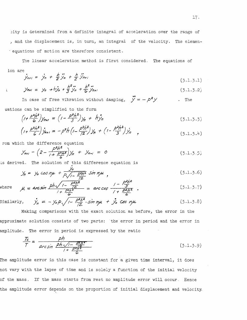
The linear acceleration method is first considered" The equations of
ion aTe
•• In case of free vibration without damping.? Y = _ p2y
rom which the difference equation p2h~ -1 (2 - /+ e.z.hZ)Yn + Yn-I = 0
T Ls derived 0 The solution of :this difference equation is
Yo
where
1) i.milar ly ;;
The
Making comparisons with the exact solution as before, the error in the
approximate solution consists of two parts~ -the error in period and the error' in
amplitude 0 The error in period is expressed by the ratio
Ts -- ::: T
ph arcsIn eh0- !if!
I+~
~he amplitude error in this case is constant for a given time interval, it does
not vary with the lapse of time and is solely a function of the initial velocity
of the mass" If the mass starts from rest no amplitude error will occur, Hence
the amplitude error depends on the proportion of initial displacement and velocit~
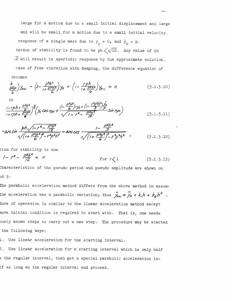
large for a motion due to a small initial displacement and large
and will be small for a motion due to a small initial velocityc
. response of a single mass due to Yo = 0, and Yo = p.
terion of stability is found to be ph < Vl2. Any value of ph
L2 will result in aperiodic response by the approximate solution.
case of free Vibration with damping, the difference equatiOE of
Jecomes
rion for stability is now z nZ/,z.
/- t - '12 =- 0 for r< 1 (3·1,,3013)
Characteristics of the pseudo period and pseudo amplitude are shown on
and 9.
The parabolic acceleration method differs from the above method in assum-
... ". L hZ .at the acceleration has a parabolic variation; thus ~+I=)lh + k,h + ~2 ~
rocedure of operation is similar to the linear acceleration method except
one more initial condition is required to start with. That is, one needs
previously known steps to carry out a new step. The procedure may be started
one of the following ways~
I" Use linear acceleration for the starting interval.
20 Use linear acceleration for a starting interval which is only half
s long as the regular interval, then get a special parabolic acceleration in-
:,erval half as long as the regular interval and proceed.
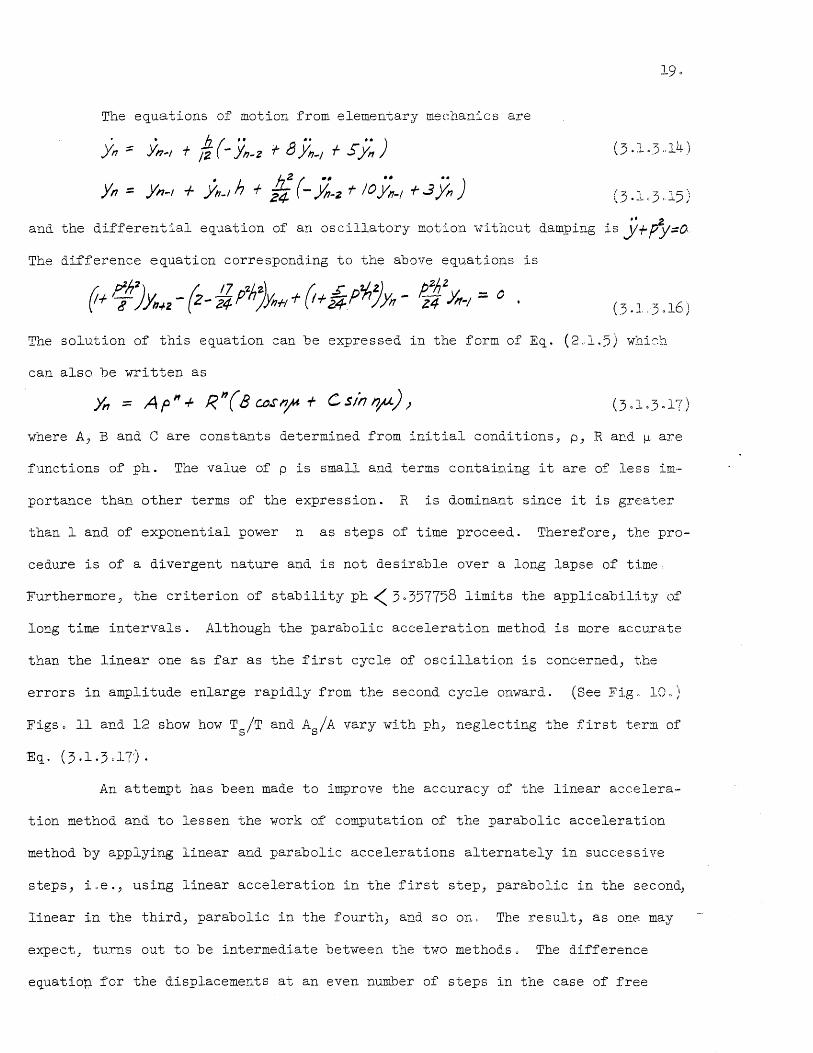
The equations of motion from elementary mechanics are
y,,;:: YI7'" f Ii (- In-z f 8 in-I f S;:)
Yn :: Yn-I + ;',_1 h + fi. (- ;"-2 t 10;"_1 + 3 in ) . t' 2-
and the differential equation of an oscillatory motion without damping lS y+py:::O
The difference equation corresponding to the above equations is
The solution of this equation can be expressed in the form of Eq. (2,.1.5) l.rhL::h
can also be written as
where A, Band C are constants determined from initial conditions, p, R and ~ are
functions of ph. The value of p is small and terms containing it are oi' less im~
portance than other terms of the expression. R is dominant since it is greater
than 1 and of exponential power n as steps of time proceed. Therefore, the pro-
cedure is of a divergent nature and is not desirable over a long lapse of time,
Furthermore, the criterion of stability ph < 30357758 limits the applicability of
long time intervals. Although the parabolic acceleration method is more ac:curate
than the linear one as far as the first cycle of oscillation is concerned, t.he
errors in amplitude enlarge rapidly from the second cycle onward. (See Fig" 100)
Figs 0 11 and 12 show how Ts/T and AsiA vary with ph, neglecting the first term of
An attempt has been made to improve the accuracy of the linear accelera~
tion method and to lessen the work of computation of the parabolic acceleration
method by applying linear and parabolic accelerations alternately in successive
steps, iue., using linear acceleration in the first step, parabolic in the secon~
linear in the third, parabolic in the fourth, and so o~o The result, as one may
expect; turns out to be intermediate between the two methodsu The difference
equatiop for the displacements at an even number of steps in the case of free
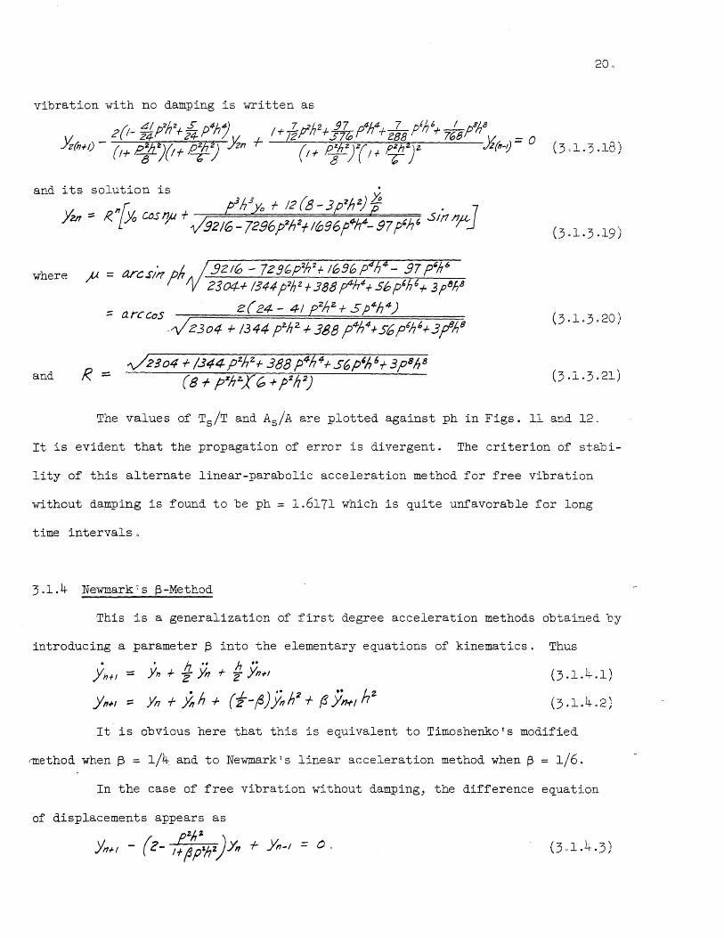
arcsin 'ph .32 ItO - 72 90P2f/z f 1696 P 4- - .97 p_;'6
where p. = 2304--1-/344 fJ2hz +388 p4h4+ S6p'h G+ 3p81;8
::: arcCos z( 24 - 41 e..zhz. + S p4-h4) (30103020)
-"';2304 + /344 p'h 2 -f- 3gB f 4h4+S6p6h'+3pll
and R :::. ~2304'" /344 pZhz.;- 388 p4l;4';-S6P'/,6 f 3p8h 8
(3·1 .. 3.2l) (8.,. pZhZ.;( 0 + p'Zh2)
The values of Ts/T and AsiA are plotted against ph in Figs. 11 and 120
It is evident that the propagation of error is divergent 4 The criterion of stabi-
lity of this alternate linear-parabolic acceleration method for free vibration
without da~ping is found to be ph = 1.6171 which is quite unfavorable for long
time intervals 0
3.1.4 Newmark~s ~-Method
This is a generalization of first degree acceleration methods obtained by
introducing a parameter ~ into the elementary equations of kinematics.
· h'· h·· :::: Yh + Z Yn + 2 Yn+1
::: Yn + j;, h -I- (i-fd))in h2 + (3 ;11.1'/ hz
Thus
(3.1.4.1)
(3·1,!.L2)
It is obvious here that this is equivalent to Timoshenko's modified
,-method when f3 ::;: 1/4 and to Newmark 1 s linear acceleration method when f3 = 1/6.
In the case of free vibration without damping, the difference equation
of displacements appears as
pZh% ~) Ynrt - (c- If fip'hZ)Yn -I- Yn .. / = 0,

iifference equation· becomes
/ . ¥1_(i-(3)p2h2 Sin nr
ri-(3)pZh'2. _ /_ (f-/3)~2h2. (l pZh2 - arc CL)S / + f3>pz Z
pseudo period with the true period" it can be seen that
dressed in a series form of
1/12, the ratio Ts/T will be closest to unity for any
~. This means that ~ = 1/12 will give the best result in
ed amplitude. is neither divergent nor convergent as time pro-
some error is involved in the response to an initial velocity.
NS that the term containing Yo does not contain any error in /
1e one with Yo is amplified by the factor ~ /- (-f - (6) pzh'Z
~pendent on ~ and ph and is free from influence of the proceeding
illustrates the variation of the velocity amplification factor
with ph for different values of
criterion for stability is p2h'Z.
~, this condition is always fulfilled for any value of ph and therefore
~y criterion need be imposed. With ~ > 1/4, no ph can possibly satisfy
'ion. Wi th fj < 1/4, the larger f3, the longer the time interval which can
For ~ = 0, the critical ph is equal to 20
The criterion for convergence is
ph < ~ (3.1.4.8)
3hows that a larger f3 permits a smaller applicable time interval. For ~ = °
22.
ocedure immediately converges regardless of the time interval used.
For problems of free vibration with viscous damping, the difference equa-
Jf the procedure may be written as
Now the error in period is not only dependent on ~ and ph, but also on r.
ain, if the ratio Ts/T is expressed in a series form as .Ji. _ phyll- rZ T : / }Z (/ Z /.! - I ) - I/- (6p + / ) t Z + 8 r.J /)2/,2. f ____ .
+ Z4- ( 1- /,:l) r I
~ will be found that (3 = (/ + ft Z - 8 r-l-J/IZ (1- 2(2)
s the best value as far as period is concerned"
(3.1.4.12)
(3.1,4.13)
The error in amplitude is dominated by the exponential factor multiplying
~he whole expression in Eq. (3.1.4.10) particularly after a long sequence of time.
Neglecting the c0efficients which combine with Yo and Yo in the expression, one
may compare amplitudes by taking the ratio
(A ) _ r( / -r# + (dp2hz _ ) rjh AS at pt=1 - e I+rfh + ~p'1hz! (3·1.4.14)
For best agreement in amplitude,
The criterion for stability is 4- (1- t:l) 1- 4f3
for r(l. Except when ~ = 1/4, the numerical procedure does not present an agree-
ment on the criterion of critical damping, greater discrepancy usually occurs for

23·
lrger time intervals. Critical damping may occur in-the numerical procedure even
or low values of r if too long-a time interval is taken.
The criterion for convergence is
There is one more restriction of this method in the viscous damping pro-
)lem. rph
A degenerate case of the difference equation will occur if / + ~ p"h 2-
is equal to +1 or -1. Under this condition the method is not workable. However,
when rph = / /1- (3 pZhz
i.e. rfh -I- (3p7.h2 = 1+ 2(3p2.h 2 )
we see that the convergence criterion is violated 0 On the other hand, when
rph / +- ~ p% h 2 = -/
the spring constant is negative 0
The ~-method is also applicable to forced vibrations as represented by
Eq. (2.1.1) with good accuracy. The error due to the presence of a forcing
function F(t) may be seen by comparison with the exact particular solution. Now,
let Yp be the particular solution of the given differential equation of motion,
Ego (2.1.1), and let yp be the corresponding solution obtained by the numerical
procedure. Analysis is made for an undamped system of single mass subject to an
applied force F(t) as follows~
Given the equation of motion
the exact solution is . . y = (Y. - YPfJ)COS pt r .Yo;, Y/,o SIn pt r y"
where y is the particular solution. p
The corresponding difference equation when using the ~-method is found
, to be
(3·1.4.19)

24.
and its solution is
where Yp is the particular solution of the difference e~uation and
· f>/;/t-(f-f3}p'h 2 = /- (i-;B);';h 2
/.1 ::: ClA"C.$I1'1 - arc ~.s /''' 1+ ~p~hZ, 1+ ~p'lh2
A = Yc - Yfo
and B = fv1+~-4)li/ {i+ l{F(f.)-f/'J+~h[F(tj)-F(t.J- (1+1('h~{jpl-YpJ) Comparing E~s. (3.1.4.18) and (3.1.4.20), we see that when h-+O, if y -+ Y , the
p p
numerical solution will approach the exact solutiouo The following comparisons
are made for different kind of forcing functions~
(a) The forcing function is a polynomial in time, i.e .
.F ( t ) == a~ -I- a, t + til. t Z f a:; t a + -- - - - (3 .1.4 .21)
then
(3.1.4022)

0.
25·
~= 1
~ = / + fz (12(3 - /)p2h2
k3 = I + t (/2(3 - / )p1.h2.,. J~O (3~O;S2.-6o~ + l)p4h4
k,. = I + i (/ 2 ~ - / ) p0/72. -f to (ao ~~ 40 ~ -+ I) p""h 4+ 2q~60 (24160;33.. $Of0(1:r25Z/-Vf'h'
ks- = / -I- :f(t2~- / )p7J?2+ 7~O {4,440f2_740(3+ t)p4h4+ 30';40f20,960(J3_3qZ40(l~t764j3-/~I/I/
f ~ 8/~/400 (;,8/4,400jJ4_Go4;8oo(fi-.s-z920j32_/,020(3 + I) p8h8
From the above we see that the numerical solution is exact for a third
!e polynomial at any value of~, and for a fifth degree polynomial when ~ =
(b) The forcing function is trigonometric, i.e.
f(t):: A S;/1 at + B cos bt (3.1.4.24)
- A . t B ccs l..t yp = p2_ a% Sin a + /2-_ b% ~
_ A s/n at + B CoS bt Jp - 2 2 sinzah z 2 si17 2 bh
? - (1+ ~s ah - 2j3sl'rJ2 oh )hZ P - (If- cosbh - 2(3sin Zbh) h 2
(c) Exponential forcing functions, as
F(t) = at at
>P :::: f2+ (log a)Z at
(3.1.4.25)
(3.1.4.26)
(3.1.4.28)
(3.1.4.29)
In all cases above, when h ~ 0, yp ....... yp' and therefore the numerical solu
~i.on approaches the exact solution as a limite
The ~-method may also be applied to other form of motion than the one re-
presented by Eqe (2.1.1). Consider the motion prescribed by the linear differen-
tial equation
y-y:::t

26.
n of which is known to be
.stant determined from the initial conditions. Applying the f3-' .
~roblem) one finds the difference equation of d~splacement to be
tl solution is
; (I + h + 2 _ ;';~h r -(t + I) le of ~ for this case is 1/6 .
. s of Finite Differences
fiS Method
, method proposed by Levy replaces the second derivative Y~ in the equa-
.)tion by finite differences, -f1 (YI1+1 - 2 y!1 + YI1-I) For a free
1 with no damping prescribed by the given differential equation
(2.1016)
.:;ituting •• I ( ) y" ::: 7i2 y,,+1 - 2 y,., + Y"-I ) one obtains
(3·2.1.1)
3 obviously identical with Newma.rkis generalized acceleration method for f3=O,
J that the treatment of initial velocity is different. The general solu.tion
. (3.2\,1) is
Yn :::: A cos I?,;t' + B s!;; tp
e fA- = arcSIn ph/;- 12::" = arc a;s (1_ ~h)
L A and B are constants determined from ini tial conditions, with ph < 2 as
ability criterion. There is no difficulty in finding A which is always equal
) Y J but trouble arises in the determination of B which depends on the o

?-rpretation of the initial velocity, or in other words, on the way in which Yl
obtained from the known values of Yo and Yo' When Yo = 0, one may assume that
Y-l' then solve simultaneously with Eq. (3·2.1.1) to get Yl' Otherwise, if
~ 0, some other assumption must be used.
If one begins with Newmark's ~-method of ~ = o for the first step in order
obtain Yl' then
f E!.),'J) h • y; :.= (/- 2:"" ~ + ~ (3.2.1.4)
l.d the result will -oe the same as Newmark! s ~-method for t' = 0, i.e., jf)
B ::: ?VI _ ~ (3.2.1·5)
If, taking the formula of elementary mechanics
y, = Yc -I- hfo re obtain • h ~il-~Yo
rhe result is, of course, less accurate.
On taking for the first half time interval
(3.2.1.8)
solving for Yl'
B =- /h / _ e;p! This is only true when )Vo= , and is only used when Yo
is uncertain.
In viscous damping problems, by replacing Yn by ih (;h.;., - y".,) and
Y~ by ;% (Yt1.f1 - 2 y" + Yh-I) in the differential equation of motion,
;/ + 2 f? Y ~ pz. y = 0 , (2.1 G 13)
one may obtain the difference equation
(3.2.1.10)
28.
:h is idential to Eq. (3.104.9) for ~ = O. The result will be the same as that
Newmarkis generalized acceleration method for ~ = 0 with exception of~the trea~
.t of initial velocityc The discussion is therefore not repeated here a
For comparison of pseudo and true periods and amplitudes of this method,
Figs n 14 and 15 c
2.2 Salvadori~s Method
This is an application of aj procedure due to Fox vibration problems 0 The
~cond derivative y is replaced by the first two terms of the central difference
{pans ion, ,. / (2 A'I-) y=p~-IzY
here a.2 and il4 are the second and fourth central differences of y
,62 y"
L::>.4 Yn :::: Yhofl - 2 yn -I- jln-I
= Yhr2 - 4 yn-tl + "YI1 - 4-Y"-I + Y" .. z ~z)
)perating then with (If;;Z- on each term of the equation
Dropping the sixth-difference terms, the equation may be simplified to
p2hZ ) YIN-I - (Z - i e.Zh2 y" f YII~I :::= 0 J+ 7r
(3.2.2.2)
which is obviously the same as Newmark's generalized acceleration method for
13· = 1/12 D (See Eq 0 (3.1.4.3).) The solution is in the form
y" = A C()S~ + Bs/n~ where %2 .s p2h2 Dh/l- ? / - /z /A = arcsin r' 77z - arc us ----=pT1h7-r":t-
/ -f P-/; I + 7Z
The constants A and B are determined from the initial conditions. For free vibra-
tions, A is always equal to Yo' while B depends on the way in which Yl ±s obtained
from the initial velocity Yo'
If the procedure is started with Newmark!s ~-method for ~ = 1/12 until Yl

is obtained, that is if
Yi = /+ ~:te ((1_ /~pzhZ)~ + 17;'] ) /Z C
the result will be the same as that given by Newmark's ~-method for ~
8 = .Yo ?VI- q
If we take the formula of elementary mechanics
Yt = Yo+hyo,
( 1+ £th2) ~ + ph Yc /2 e 2 B = then
29·
(3.2.205)
= 1/12.
(3·2.2.6)
which involves more error than the previous result. However, the accuracy of the
velocity response can be improved if the initial velocity is properly treated.
In the case of forced vibrations with a forcing function ~(t), the
difference equation of Salvadori~s method becomes
!tNt -(z- S1i~~ + ~-I = /zt: o/1:j{F(tM,)+ /oF(tll)+ F(tl1-t)}
which is again the same as Newmark's method for ~ = 1/120 (See Eq. 3.1.4.19).)
This method is accurate to the order of h5 provided that the motion starts from
rest. If the motion begins with a finite velocity, the treatment of the initial
yelocity for the difference equation determines the accuracy. The discussion of
this method is included in Newmark's method in previous and later chapters, and
is not ~estated here.
Salvadori treats the damped motion problem in the same way as Levy does
by transforming the damped motion equation into an algebraic equation by the
substitution of central averaged differences for the derivatives. The difference
equation thus formed is
(1+ tph )y,,/-I - (2-pzh2)y" f (1- rph) Y"--I ::: 0 (3.2.2.10)
which is the same as Eq. (3.2.1.9). There is a difference in~lprocedure when
applied to a multi-degree-of-freedom structure but it does not affect the nature
of the error s .

3 Houbolt 1 s Method
Houbolt 1 s method is based on the assumption of a cubic curve for the dis-
~ement of the moving body, considering that four successive ordinates can be
sed through by a cubuc curve. With this assumption the following difference
ations for the final derivative may be obtained 0
)/17 == ;2 (2 Yn - 5 Y"-I + 4 Ytl-2 - Yh-3)
)ttl = ih (/1/11 - 18 YI1~1 +- 9 y,,-z - 2 Y"·3)
(3.20301)
(3 0 203.2)
The derivatives at the third of the four ordinates are sometimes of use
.d are as follows ~
Yn = fz (Ylltl - 2 YI1 + YI1-I) in = {Ph (2 y",., -I- 3 y" - 'YI1-' + Yn-2)
(302.3·3)
(3.2.3.4)
For free vibration without damping, substitute Eqo (3.2.3.1) into the
[ifferential equation of motion
(2.1.16)
The following difference equation is obtained.
Its solution is
y" = C, XI" + Cz XZh r C3 X,/'
where xlJ x2' and x3 are the roots of the equation
(Z + fth 7) X 3 - 5 xz. + 4 'X - I = 0
It can be shown by the theory of equations that this equation contains one real
root and two conjugate complex roots for any value of ph. Therefore the solution
has always an oscillating nature and no criterion of stability governs the choice
of the time interval J although the amplitude may be damped out very rapidly as
time proceeds (see Fig. 18). Eq. (3.203.6) may also be written in the form
y" = A e -apt f e-bpt ( 8 ~: cpt + C SIn C,f)t) (3.203.8)
where a, b, and c are all functions of ph. Here A, Band C are constants deter-
~ined from the initial conditions" The first term of the equation is negligibly

310
small while the second term multiplied by e-bpt
is dominant. Tab~e (30203.1) lis~
the numerical values of a, band c for various ph, Fig. 19 shows the ratio of
pseudo period to true period Ts/T, and Fig. 20 shows the ratio of amplitudes As/Ao
The disadvantages of this method are two-fold. First, it needs one more
i~itial condition to start with 0 Although this can be found by taking account of
the initial acceleration it also involves effort to trace the back differences
including the simultaneous solution of equations Eqso (3.2.3.1) to (30203.4). If
the initial conditions are awkwardly treated, e.g. by making the assumption that
the fictitious displacements at t = -h and t = -2h are zero, the error introduced
by these erroneous assumptions would be greater than that of the method itselfo
The step-by-step evaluation of succeeding displacements cannot proceed in a
straightforward manner until three initial displacements have been established.
Secondly, the amplitude of a slightly damped system decreases so rapidly even for
a time interval of about one-sixth of the natural period, that the amplitude is
reduced 50 percent after one and one-half cycles of vibration. (See Fig. l~.)
Finer time intervals and thus more computational effort must be used to reduce
the damping effect of the procedure.
For free vibration with viscous damping, the difference equation of this
method becomes
(2-1- fl'ph+p2hzjy" - (5+ ~rp/;)YI1_1 + (4+3rph)y"..z. -(1- jr;:;h)Yh-3 = 0 (3.2.3.9)
The solution is in the form of Eqo (3.2.3.8) ~ith a, b, and c functions
of r and ph. The criterion for stability becomes
Values of a, band c are listed in Table 3.2.301 for various ph. The ratios of
T"s/T and AsiA are also plotted against ph in Figso 19 and 20. It can be seen
that the error in period increases with time interval h and the damping factor r.
The amplitude ratio is less than 1 for systems with slight damping and greater
than 1 for system with higher damping factor r.

32.
20301 -- Values of a, b and c of E q. G. 2 . 3 08)0
ph a b c
005 1.5587 0.0318 0.9208 1.0 0·9024 0.0981 0.8016 1·5 0.6724 0.1461 0.6940 2.0 0~5494 001733 0.6047 2·5 0.4706 0.1868 0.5325 3·0 0.4149 0.1922 004740
J.25 0·5 104176 0.2074 0.8808 100 0.8185 0.1963 0-07357 1.~ 0.6108 001959 006213 2.0 0.4987 0.1941 0·5350 205 004262 001882 0.4687 3·0 0·3746 0.1820 0.4165
0050 005 1.2436 0.3766 0.8312 100 007304 002787 0.6836 1.5 005528 0.2371 005694 2.0 0.4547 0.2122 0.4871 2·5 003900 0.1942 004258 3·0 0·3435 0.1799 003785
= 0·75 0·5 1.0018 0.5638 0.7848 1.0 0.6349 0·3544 0.6439 1.5 004960 0.2739 005307 2.0 0.4142 0.2302 0.4519 2.5 0·3584 0.2019 0·3945 3·0 0·3173 0.1815 0·3507
3 Numerical Solution of Differential Equations
3.1 Euler's and Modified Euler Method
Euler's approximation is based on the assumption that if y is expressed
s a function of x by the equation ~~ = f (x .. y) , the increment in y corre ....
ponding to an increment, A x, in x is given approximately by the equation
6y = !(X"Y)AX , the value of f(x,y) being that at the beginning of
the interval .Ax 0 Applied to the problem of free vibration, with damping,
.. • z governed by the differential equation y + 2 rpy + p y ::: 0, the formulas for new
displacement and velocity at end of a time interval are found to be
:11 = YD + h~
33·
and (3·3.1.2)
When this procedure is carried on in a step-by-step manner, using the displacement
and velocity found from the previous time interval as the initial condition of the
new time interval, the difference equation becomes
The solution of this equation is ~ r,Yo + ..sln~) y" R"(YfJ US~ + 12 (3.3.1~4) - ¥'I-/ 'Z
where R. VI- zrph + phZ - (3.3.1,,5)
fo = . I'h~ - arc: cas /- rph (3 03 01 .6) and arc-Sln R. R
The error is of the second order and the amplitude damps out gradually
with time~ There is no limiting criterion for stability in case of free vibration
with no damping. Any time interval will obtain oscillatory response 0 For free
vibrations with damping, the criterion for critical damping is the same in the
numerical solution as in exact solution, ieee aperiodic motion at critical damping
occurs when r = le
Figse 21 and 22 show the errors in period and amplitude at pt = 1 for
various ph.
The modified method of Euler takes the true average value of dy/dx over
an interval instead of dy/dx at the beginning of the interval for the equation
&-4~ -- I"(x' y)' ~ , This method gives a more accurate value of the increment of
y due to increment of x than Euler1s original method and the error is of third
order of (~X)3e This method may be represented by the formula
Li y = i ( ~ / + ~II)
'W"here A ~ = f ( X()" y~ ) L1 X
~II = f ( Xc -I- ~ X / Yo + ~ Y ) LJ 'X
When applied to the problem of free vibration with damping, the displacement and

velocity at the end of an interval now become
)',,+1 == (1- ~))liI + (/- tph) h Yn YI1+1 ;:: [i-zrph- (i-zrZ)p2hz];in + (-I f rph)p2h yn
This procedure may be represented by the difference equation
the solution of which is found to be ~ Yo
Yn ::: R "( ~ CoS o/A + :$1: t T Sfn 'J# )
where R = N / - 2rj:Jh + zr2p2hZ - t f~h3 + i f~h4-~ = arcSin ph(i-rp/,)A/'I-rz- =~Ct;s l-rpJ,-rt-r2)pz/,z
R R.
(303 .. 1.8)
(3·301·9)
(3.3.1.11)
(3.3.1.12)
Again, there is no limiting criterion for stability in the case of free
vibration without damping, but the amplitude of vibration seems to damp out
gradually if the range is carried too far. In damped vibration problems, the
numerical method has the same criterion for critical damping as the exact solutro~
Figso 23 and 24 show the errors in period and amplitude for various ph
of this method.
3Q302 Runge, Heun and Kutta1s Third Order Rule
Various formulas have been devised for numerical integration of the
differential equation ;~ = f(-x,y) by Runge, Heun and Kutta. These methods,
accurate to the third order of ~x, are summarized as follows~
where
1. Runge1s Original Formula~
~ y ::: ~ /1// + j r i ( L:/ + ~ /11) - A/III}
At = f (XI Y ). ~ X
c/I = f ( ;X + ~ X; Y + Lj/ ) .. LJ I(
AlII = f ( 'X + L\ X;, y f ~ 1/ ) • Ll X
If'''l = f (X -I- i~ 'X.; Y + flll) .. ~)(

where
where
2 0 Reun~
~ y :;::. it ( L::/ T 3,6///)
~/= f(X~Y)'~X
~//:::. f(X+ f~~; y + jc;/),,6X t1111:: f (X + j ~ X., Y + j 6/1 ' A -X
3" Kutta i s Third Order Rule:
.6. y ::. ~ (a/ - 4~// + ,6///)
~~ =: f(X~Y)' LJI(
~// = I (?( + f~xl y+ f ~/). LJX
~///= /(X+AX;, y+ 2LJ;'I- ill)'AX
All these formulas when applied to free vibrations with or without damp-
ing yield the same resultso When applied to forced vibrations, their results have
slight discrepancies but all contain errors of the fourth order 0 It is hard to
say which of the above formulas is best because the agreement with the exact solu-
tion depends on the type of forcing function, damping coefficient and time interval
in a very complicated manner.
Considering the free vibration problem with damping, the follDwing
discussion is common to all three of the methods above mentioned 0
The displacement and velocity at end of a time interval are found to be
x:; (i- i p1hZf f pll)Yo + [I-rph - i{t-4/Z)pZ!l1.j hfc (3 0 3. 20 4)
>1 := - f- 'fh - i(;-4 /1 )Pt/'j p2hx, f {I-2 rfh -f(;-4r 1011,1+ j t(J-2r~?J/lJjo (3.3 0205)
These e~uations, if applied successively by using the final value of previous
step as the initial value of the new step, lead to the difference e~uation
y;,tl - [z-2tph-(t-Ztz)p2hl..;. f(3-4tt)pJ/;])h
+ {;- 2 rph -f 21t;PZ/,Z- .jr~JhJ-It(i-8r~ptl-h4_ i ;;s/rS+ 16 p1hjYn_, = 0
(30302.6)

The solution o£ this e~uation is
where
As before, these methods have no limiting criteria of time interval for
stability in problems of free vibration without damping, nor there is any dis-
crepancy in the damping coefficient r at the point of critical dampingo
3.303 Kutta's Fourth Order Rules
where
where
The formulas with -error of order (~x)5 derived by Kutta are~
1. Kutta's Simpson's Rule
6 y = t ( a/ + 26/1 + 2 ..6 //Iof A //1'/)
t:/::: !(XDI/O)·Lj"X ~/I = f (")(0 + i.ax/ Yc + tl:ll) , AX
1::.111 = f (I<~ -1- t tJX" Yo + -i Ljll) .. L1 X
~III~ f ( -;(6 + t:J X / ./0 + L:/I/) • Ll. X
2. Kutta T s Three-eighthRule
~ y = t C ~ / + J ~/I -; 3 ~III ..,.. A, 1111 )
tJ/= f(~/~),tj")(
A/I: f(X()-I-fAX/YoffA/)'~X
LfI':::: I (X(;+ j-~)(, Yo + A//- j A/)' AX
/:!IIII =- f ( Xc + Ll X I Yo + ~ III - ~ II + Ll' ). Ll X
(3·3·3·1)
(3·3·3·2)
No difference in results between these two rules occurs when applied to
free vibration problems 0 For forced vibrations the results will differ slightly
but both are of the same order of error. The agreement with the exact solution

37·
varies with r, ph and t.
The displacement and velocity at end of a time interval in the problem
of free vibration with damping are found by either of the two rules to be
)', == {I - -j pZh7f jrp3h'f-i4 (1-4r2)p4h4] Yo
+ [1- (ph - f(t-4r Z)pZhZ-f i (1- 2rz)p3h3
] hjo
Yt :::! [-I + rph + t{t-4-(2)p1.h 2- i (1- 2/ 2)p3h3
] p2hyo + [1-2rph- i(I-4r2)pZh2+ ¥(t-zrZ)pJh3
-f .g(I-/2r~/forjp4hji
This may be put in difference equation form for the step-by-step method, as follows
Ynfl -[2-zrph -(1-2t1p0/72f J(.3-4rzJp3!i;+ fz (1-8r2-1- 8 r4)p4),1Yn
-f [1-2tph-f 2fj}h'2-J rJpJ/,3f lr"p4h4 + fz (t-4r2)pS!r5 - fi(I-~r2)p'h"- fitp 7h7f ..s~'fe;;e)Yt,_1 == 0 (3·3.3.5)
The solution is found to be •
",{ ryo + i- ' ) Yn := R fi CtJ.!' nM 1- '" / 5117 nr 7· 'V / - rt.
where R == [J- zrph f 2tzpzh 2 - -jrip3h3 f J r4p4h4
f Ii (;-4r1p·h·-Iz{!-~rz)pt.ht.- fzrf'IJ7+ ?;a?WJi .M- :: arcsin ph[l- rph- i(I-4rZ%/;2+[(I-zrtJp'/,3j ~
__ / -I'ph - i (-ztz}po/, 2+ f(3- 4rz)eihJ.;- -f4 (t- 8rZ+8r1e"/;4 ~~s K
(3·3·)·8)
Like all other methods of this kind, the fourth order rules have no
limiting criteria for stability. Any time interval can be used according to the
accuracy desired. When the system reaches its critical damping, ioeo, r = 1, the
numerical solution becomes aperiodic. A difficulty associated with the method is
that the amplitude will gradually damp itself out even in the case of an undamped
system, and the method is therefore not desirable for a long period of time.

IV. DISCUSSION
4"1 Accuracy
It is usually convenient to compare the accuracy of various methods by
the order of time interval h involved in the error produced. The final displace-
ment over a time range computed by numerical methods can be expanded into a
polynomial of ph and then compared term by term with a standard power series
-:3.~ri ved from the exact solution 0 The error occurring in each step of the step-by-
step method may thus be observed, especially as to the order of ph involved.
Considering first the case of free vibration, with damping, which is governed by
the differential e~uation
J + 2rpy + p'y = 0
may be expressed in a power series for a time interval h
Ynfl:::: Yn [I-irl/'Z+ ff¥JJ+ !4(1-4rZ)p4-h+- k(I-z.rzJfhS., .... ] f jnh{t-rph- i{t-4,1pfl+ tv-Zt3)ph3+ fza (1-/2 tZ:; /!t;r4),P~h4+ •.•• :1 (4.1.1)
The following is a collection of e~uations which show the accuracy of
different numerical methods~
Constant acceleration method~
Newmark'S ~-method:
1h+I:::: [1- i;rh'l.+ 2~rp3hJ- i(4~r2-;B )p4h~ f i(4~rJ-(3r- 4~2r)prJ,.s- i(4(3~~r-g~z'Z+f1Vf'h'f .-J/J,
+ [/- rplr+ (4-lrZ-f.;)fi-;~- 4(r~ - 2ftBJ,ihJ + (4r(; - 2f'P - ~r~2 + tB z )p4h4 + •... J 17ft,
(3·1.1.13)
(4.1.2)

ttat~
For ~ = 1/4 (Timoshenko 1 s modified methodo)
Y,,+I = [1- -j p"h 2 f f pShi_ ... "JJn + [1- rph - f(t-4r~)pZh%-I- .·.JhY" For ~ = 1/6 (Linear acceleration method.)
Im-' = [1- j pZiJ2+: pdhJ-f -!z(1-4r2)p4h4 + - _ .. ] .Yn + [1- rph - i;(;- 4rz)f zh;.+ ?j(Z- ft)plj,1+ .... ] hy"
For ~ = 1/12 (Salvadori's method.)
/1rH = [1- f;'/l+ffhJ+ /;j{t-4t;}p4/,4_ i('-3r~flh5"+--JYn + [1- rph - ii(l- 4(2)pZj.,z+ .... ] hYi7
For ~ = 0 (Levy's method.)
y,,+1 = {I- i f 2,42] Ji7 + (1- "ph] hy" Parabolic acceleration method:
Yn~1 = {I- -jp¥,Z+ J (ltr+ 24.{I-4f9p~h4+ 1;;8(.sb3-/g2tVr~~ ···JYiI + [;-rph- t(i-4fVp2h2+ f(;- 2!~rh3_1z.{!-I"r2fgbl~)llh~ .. --j;,y"
Houboltis method~
jn+1 :::: {I- -j pZh~+ {-Ph 3 -I- /;(i-4rzJp4-~ 4-+ - -- -] Yn + [I - rph - f(l- 4rz)p-zh z i- f (1- zrz.)/}hJ-f- ----] hi
Euler T s method~
Modified Euler Method~
P!/'-' . Yh-r/::= (1- z) Yn + (1- rph)~Yn
Runge, Heun and Kutta's third order rule~
Kutta I S method:
/n+1 == [1- fp~2+ Jp31?~f!4 (1- 4rVPh 4] Yn
f [1- rph - t(t-4r~p% '2+ f{l- 2ri}p3if J h~
39·
(4.1.3)
(4.1.4)
(4.1.5)
(4.1.6)
(4.1.7)
(4.1.8)
(3·3.1.6)
(3·3·2.4)
From the above listings of equations for v~us methods, one may observe
10 The constant acceleration, linear acceleration and parabolic accel
eration methods have, respectively, an accuracy of the order of h2, h3 and h4 in
Doth displacement and velocity. The accuracy of Newmark's ~-method depends on

40.
2. Levy's and Houbolt 1 s methods have, respectively, an accuracy of the
crder of h2 and h3 in both displacement and velocity responses.
3. Salvadori's method is of order h5 only in displacement response and
only for undamped systemsc If r and Yo are not zero, this method is only of h2
accuracy unless a good interpretation of Yo is made.
4. Euler=s method is of the first order; modified Euler metnod, second
or~er; Runge and Heun, third order; and Kutta's Simpson's rule or three-eighth
ruJ'2 j :fourth order generally.
5. In some special cases the accuracy of the above methods may be pro-
moted. on.e more order. These will be listed in Chapter 5.
In t,he case of forced vibrations, the error which enters the particular
solution also governs the accuracy of the method since it determines the constants
for the ini ti.al conditions. As before, Newmark 1 s linear acceleration method is of
'thi!'d order accuracy :for any system with or without damping. For an undamped
system startir_g at rest, Salvadori' s method has an accuracy of fifth order. Eulert~
moiified Euler, Ru~ge-Heun and KuttaTs methods are still of first, second, third
and fO~ITth order respectively.
The comparison of errors by polynomials is only good for ph less than 1,
~::ecause the error would otherwise be dominated by the higher powers of ph which
would vit.iate the analysis. Nevertheless, usual practice indicates that a large
tim.e interval, say from 1/4 to 1/2 of the natural period of vibration (ph=1.5708
to 3.1416) is highly desirable in rapid and rough estimations. The effect of
l.a:rge tim.o::? intervals is shown in the graphs of Appendix 30
4.2 Propagation of Errors
The preceding article concerns the accuracy of displacement response of
various methods in one single st~p of operation, the error indicated in the

41.
expanQed polyn.orr.ial being compared with a common initial condition. :But if' step-
-by-step eval~lations are set up, with a common initial condition for the first step,
t]:le j_ni tial condition of the second step will contain error which is different in
vaTious methods After a chain of steps is completed, the error propagates in
different 'iiiays, divergent or convergent, accumulating or self-eliminating, as a
fru:.ction cf -t,ime, length of time interval, natural frequency and. damping factor.
Sho,,;,,-n in previous chapters are the equations for Yn and in Ar:pendix 3
a:ce graphs 0::: T~/T and. AsiA for various methods. These may serve for an estimate
o£ the propagatioTI of errors.
Errors are of two fundamental types, error in period and error in ampli-
t1.ldeo The error in period or in frequency is solely due to the discrepancy in
phase angle ";\"hich is directly proportional to the lapse of time. The err'or in
amp2.it~i.de, on thE: other hand, chiefly depending on the factor Rn in the equations
O-P --,'"- "Y n) is aLi. ex:pcnential function of time. From the equations for Yn d.erived and
listed i'" Chapter 3 ; it is evident that the condition for no error in period is
p11 = ~l and that fer no divergent error in amplitude is Rerph = 1. All pseudo
periods and pseud.o amplitudes have been compared with true periods and true ampli-
tv.des i:o.. tt~e rreceding chapter. The ratio of periods is given by the relation
Ts = ph~ T r (~·.2.1)
ar'.c. tr}:; aru;p]_i tud.~s by As/ A c There are two ways of comparing the ampli tud.es. The
f:Lrs-s one CO:!.lCeTns the ordinate of the envelope which prescribes the period.ic
~r.'esponse.~ Ylhi.le t.he se:::ond way takes account of the peak amplitude in the first
cycle of 7i"t~ation;J sabject to a certain initial velocity 0
In the :irst i.'1ay of comparison, one finds that
== e -rpt (4.2.2)
:c.eglec~;j_n.g tt~2 magni.fyieg effect of initial velocity in some cases.
Since ~he ratio of amplitudes is not constant with time, it is reasonable

L~-2 0
tc compare the methods at a certain designated time, say, at t lip, i.eo pt = 1.
Note that the ~atio AsiA at pt=l here does not mean the comparison made
with the pseudo amplitude actually computed which is not only affected by the
factor R, but also usually by the change in velocity response. The velocity re-
s"Donse depends on ph as stated in Art. 3,1.4, and sometimes on the initial
displacement as i:: Eq. (3.1.3.18). However; when the time interval is not clost::
tc the criterion. of stability; this error in amplitude due to initial velocity
response is o~ a constant nature, doing much less harm than the exponential
factor R after a considerable lapse of time, and. is not taken into consideration.
'rherei'ore the ratic As/ A for the envelopes of the periodic curves is still ~~seful
for judging the convergence and divergence oi' errors.
Nevrmark! s t3-method for all values of ~ from 0 to 1/4, together "loli th
T:'!..mos:::tenko; s TIlod.ified, NewlIlark i s linear acceleration, Levy: sand Salvadori i s
methods, have As/A = 1 in free vibration of an undamped systemo Constant and.
para-bolie acceleration methods are the ones which have di"'lergeng amplitudes I;\'hile
the others, including Roubol t's, Euler 1 s, modified Euler, Runge IS, Heun; sand
Lutta's methods, have convergent amplitude although the rapidity of d.ivergence or
convergence is different.
The presense of damping may add complication to the analysis 0 Plottings
of As/A at pt = 1 shov.rl.1. in Appendix 3 are self -explanatory 0 The relation bett.Teen
As/A at any time and As/A at pt = 1 is shown in Fig. 29.
In the second method of comparison, peak amplitudes in the first cycle
of vibration due to an initial velocity Yo = p are compared and sholNll in Appendix
3. This comparisoL may be of more interest in p~actical problems of vibration
since it gives actual amplitudes of periodic motion 0 The magnifying effect on
the sine term of the general equation is generally taken into consideration except
in the parabolic acceleration method and Houbolt's method where the magnification
factor depends also on the treatment of initial conditions 0 Note that the magni-
tude of the peak amplitude does not depend only on the value of R, but also on the
error in period as well 0
Error in period is, as a rule, constant for a given ph. Generally
speaking, the ratio-T IT increases or decreases with the broadening of time inters
va.l 0 Ts/T) 1 indicates a larger pseudo period or a retardation of phase angle
and vice versa.
4.3 Stability and Convergence
The apFlicability of different available techniques places some limita-
tions on the time interval used, not only as regards accuracy, but also as regards
stability and convergence. All acceleration methods have a_limiting criterion of
~cni,rergence because of their iterative Frocedure. All acceleration methods"
except Timoshenko's modified method,_ also have a limiting criterion of stability
beyond which aperiodic response will occur. This has been discussed in Art. 30_1.40
(See Eq. (3.1.407) and (3.1.4.8)0) Larger values of ~ provide a wider range of
time interval for stability, but a shorter range for convergence. On the other
hand, when ~ = 0, -freedom from the convergence criterion is obtained at the loss
of range for stability. The presence of damping will also affect both criteria;
the greater the damping factor r, the shorter the range of time interval available.
The difference equation methods have generally no limiting criterion
for convergence because of the nature of the procedure. However, a criterion ror
stability still governs those techniques which have been discussed in previous
chapters. Levy's and Salvadori's methods have the same criterion for stability
as that of Newmark's ~-method when ~ = 0 and ~ = 1/12 respectivelyo The
Houbolt method criterion for stability has been given in Eq. (3.2.3.10).
The methods of numerical integration described in Art 0 3.3 have the

44.
~voiding limiting criteria both of stability and convergenceo The
~ interval may therefore be made according to the accuracy desiredo
visable to use any time interval greater than lip, that is, ph ;> 1,
;ry misleading results may be obtained because of the fact that higher
n will dominate the solution .
. 'he criterion of critical damping in the exact solution is r = 1; while
of the numerical solutions have the same criterion. Those which have
_terion of critical damping are: Timoshenko 's modified method or' NewmarKls
for t3 == 1/4, EulerTs method, modified Euler method, Runge's, Heun!s and
lethods. In most of other methodscri tical· damping occurs even when r< 1.
ar acceleration method, Salvadori's method, Levyts method and Newmark's
i (with the exception of t3 == 1/4) are all of this group. The criterion. of
stant acceleration method may be higher or lower than the actual criterion;
Lng on the product of the natural frequency of the structure and the tim.e
al used. Houbolt t s method generally exhibits periodic response for alJ_
of r and ph except in some cases when r is greater than 0.94 and ph very
Fig. 30 illustrates the criteria of critical damping for various techni
The region above a curve is that of aperiodic response, while the region
r a curve is that of periodic response.
Procedures of Operation
Acceleration methods require an iterative procedure starting from an
,sumed value of acceleration and arriving at a derived acceleration by use of
ne equations of motion until a close agreement is obtained between the assumed
Lnd derived values 0 With a proper choice of time interval; three of four trials
for each interval of time will usually be sufficient to reach convergence in a
multi-degree-of-freedom system. The time consumed in completing a step by an
electric desk co~puter is about nine minutes for a two-degree-of-freedom system
~enty minutes for a five-degree-of-freedom one after the equations are
a routine form is madec The result of each step is self-checking except
:ial case of ~ = 0 in Newmark 7 s ~-method. Both displacement and velocity
as a supplementary help for giving a clearer picture of motion and for
Difference equation methods are faster because displacements are directly
from the difference equations and no extra work to obtain velocities is
However, they suffer from the absence of self-checking procedures unless
cional device is provided 0 For problems of mul ti-degree-of -freedom systems,
suggested a recurrence-matrix solution in which the equations of motion
~ressed in a recurrence matrix equation and solved by inverting the matrix .
. or1 expressed the equations of motion for every three adjacent masses so
~ach equation contains only three unknowns and may be solved by relaxation,
, and error, or successive approximations. The evaluation of displacements
six significant figures for a five-degree-of-freedom took approximately ten
,tes ij,fter the computations had been standardized)6)
Rungeis and Kutta~s methods are the most time-consuming as far as the
of an electric desk computing machine is concernedc It takes more than thirty
.lutes to complete a step by Kutta v s fourth order formula for a two-degree-of-
eedom system. Furthermore, since there is no self-checking of calculations,
Lstakes may easily be introduced into the computations due to the intricate work
f cross-substitution in the procedure 0

v 0 CONCliUS IONS
The general results of this study are tabulated on the next page (Table
in which the advantages and disadvantages of each of the available techniques
.isted. Graphs showing the errors in period and amplitude for a range of time
~val from 0 to about half of the natural period in various methods are given
he end of this dissertation. It is therefore possible to choose a suitable
Lnique for a specific problem according to the accuracy and amount of work re
~ed" In general, the larger the time interval, the cruder the results. Values
ph less than 1 always give reliable results for all techniques, but variations
.1 be great when ph)l, and these graphs. may be found useful fOl;" judgement when
Lng large intervals.
In orqanary problems of Vibratory motion, Newmark's ~-method is most
.luable .because of its flexibility in application. The choice of ~ime interval
iy be made for the desired rate of convergence and accuracy by adjustment of the
- parametero The linear acceleration method, a special case of the ~-method for
'31/6, is most consistent in degree of error when the motion is that of forced
ribration with damping, with initial displacement and velocity. Timoshenko;s.
method is best applied to an undamped system when the response in amplitude is
importantc The constant acceleration method and Euler's method are not advisable
owing to their inaccuracy. If the masses in motion are not damped and have no
initial Velocity, Salvadori's method is most rapid and accurate. For rapid and
less accurate work, Levy1s method may prove useful, but care should be taken in
the treatment of initial velocity. Runge and Kutta's methods ~e noted for their
accuracy and generality in application, having no restrictions with respect to
stability and convergence, but they are handicapped by the tedious procedure which
is not generally desirable for use as an ordinary engineering design technique,

Table 5.1 Summarized Result of Analysis
Order of Accurac~ Item Techniques Displace- Velocity Forced Amplitude
Noo ment Vibra- when r=O Response Response tion
10 Constant Acceleration 2nd 2nd divergent
2. Timoo Mod. Acce10 2nd 2nd 2nd constant Newmark t3 = 1/4 (3rd when (3rd when (~rd·when
r = 0) r = 1/2) r = 0)
3· Linear Acceleration 3rd 3rd 3rd constant Newmark t3 = 1/6 (4th when (4th when
r = 1/2) r = 0)
4. Parabolic Acceleration 4th 4th 4th divergent
50 Newmark's t3-method Depends on f3 constant
6. Levy 2nd 2nd 2nd constant Newmark f3 = 0 (3rd when (3rd when (3rd when
r = 0) r = 1/2) r = 0)
7· Salvadori 2nd 2nd 2nd constant Newmark f3 = 1/12 (5th when (3rd when (5th when
r = 0) r = 1/2) r = 0)
8. Houbolt 3rd 3rd 3rd conv~
(4th when (4th when r = 1/2) r = 0)
9· Euler 1st 1st 1st cony. (2nd when r = 0)
100 Modified Euler 2nd 2nd 2nd conv. (3rd when r = 0)
11. Runge, Heun 3rd 3rd 3rd cony. (4th when r = 0)
12. Kutta 4th Order 4th 4th 4th cony. (5th when r = 0)

48.
Table 5.1 -- Summarized Result of Analysis. (Concluded)
Item :Ci'iterion of Criterion of Self'- Time No. Stability Convergence Check- Consump-
in~ tion
1. ~Cl· (3.1.1.13) no no less
2. no rph+ip'J.h2 < / yes fair
3· Eqo (3.1.3.13) tph t ifZh1 < / yes fair
4. ph < 3.357758 ph< 20828427 yes more for r = 0 for r = 0
5· Eq. (3.1.4 015 ) Eq. (3.1.4016) yes fair
6. ph < 4(1- rz) no no less
7· ph < ~ (1- ,Z) no no less'
8. ECl· (3.2.3010) no no l'air
90 no no :.~.no less
10. no no no fair
11. no no no more
12. no no no more

APPENDIX 1. NOMENCLATURE
The letter symbols and notations used in this thesis are defined as
follows except otherwise noted.
A = amplitude of the moving mass.
As = pseudo amplitude obtained by numerical methode
A, B, C, = constants determined from initial conditions.
a, b, c, = coefficients used in equationse
e
F
h
k
n
= 2.7180 ... base of 'natural- logarithms
= forcing functione
= time intervalso
= constants.
= number of time intervals taken in the step-by-step evaluation, or subscript to designate displacement function at a particular time, as Yo' Yn or Yo' Yn ·
p = circular frequency of natural vibration.
r = factor of viscous damping in terms of p.
-'T = natural period of a general system, in general T = 21tjp.
Ts = pseudo pe.Liod of vibration obtained by numerical method.
t = time.
t = time corresponding to end of nth time intervale n
X = variable in general equations.
y = displacement of mas s
y = first derivative of displacement with respect to time, i.e. velocity of mass.
y = second derivative of displacement with respect to time, i.eo accelera-tion of mass.
y = exact solution of differential equation 0
Y = particular solution of difference equation for numerical methods 0
n or
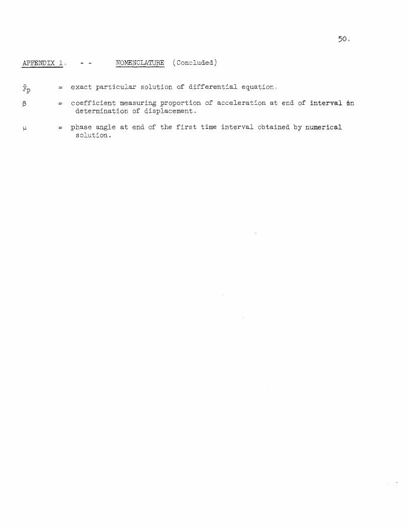
APPENDIX 10 NO:MENCLATURE ( Concluded)
Yp = exact particular solution of differential equation 0
~ coefficient measuring proportion of acceleration at end of interval mn determination of displacement.
= phase angle at end of the first time interval obtained by numerical solution.


APPENDIX 3. -- FIGURES

-P ~
~ ill U
3
2
1
~ 0 P-l en ·rl (::l
-1
-2
-3
, ,,~ /
~/
I
ph == 1.0
~
I ph = 0.5, !
~ ,/" ~ ,11/ I ~ r- -~ g 10" -
- .... ........ " ~\ i· v//' 10--" ........
" ~ , .... f\ t/ " \
~\ j" J , ....
/' 1 2
3 '\ 4 5 6// /7 ~ .,~'
~/
"\ /' V / "",/' ~ " ......... .......... ~ ......... )
'~ / / \ ~ r-/ / ,
V 1\ .
'\ ~ V
-~-
Fig. 1 - Constant Acceleration Method: Displacement in First Cycle due to Yo 1. Free Vibration. No Damping.
~ /
/ I
I
I
I
I xact I ~..- l
I
i
I
I
-- -
pt
\Jl \j.I

E-I ...............
Ul E-I
1.
1.
1.
1
1 )
o 0·5 1.0 1·5 2.0 2·5 Fig. 2 - Constant Acceleration Method: Error in Period
3.0 ph
\J1 +""
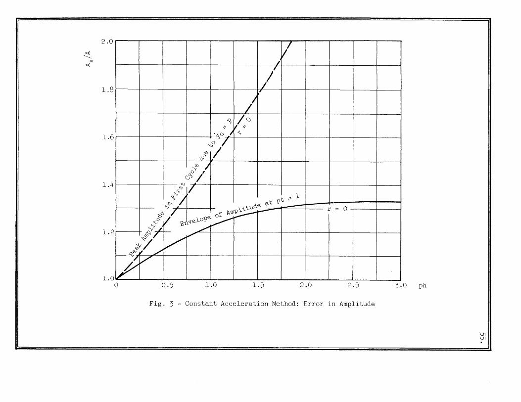
i. ----:~================================~ .i
~ ill
<r:
2.0
1.8
1.6
1.4
1.2
1.0 o 0·5 1.0 1·5 2.0 2·5
Fig. 3 - Constant Acceleration Method: Error in Amplitude
3.0 ph
V1 V1
I' 'I

1.2
1.0
0.8
0.6
0.4 / I
/
~
0.2 p
~ ill U 0
.I I
"I m ~ ~ w 'rl q -0.2
-0.4
-0.6
-0.8
-1.0
~ ~ ,~
~ h Exact
~/; Irl / ,f '\\
l\ Vi, [7 J~ ~ ph = 0·5 V
1/ [\\G. .~ Vj V \\1 ,/ ~ \ il V~h=l.O 1\ \\
'~\ I VI ,II 1 2
3 '\\ 4 t::;
6 'I /7 ./
i\ ,I \~ ~\ VI / I '\ \\ /J /
'~ ~ JI/ V
'~ \
~ ~ V '\
Fig. 4 - Timoshenko I s Modified Method (or Newmark I s Method for !3 = 1/1+): Displacement in First Cycle due to Yo = p. Free Vibration. No Damping.
pt
\Jl 0\
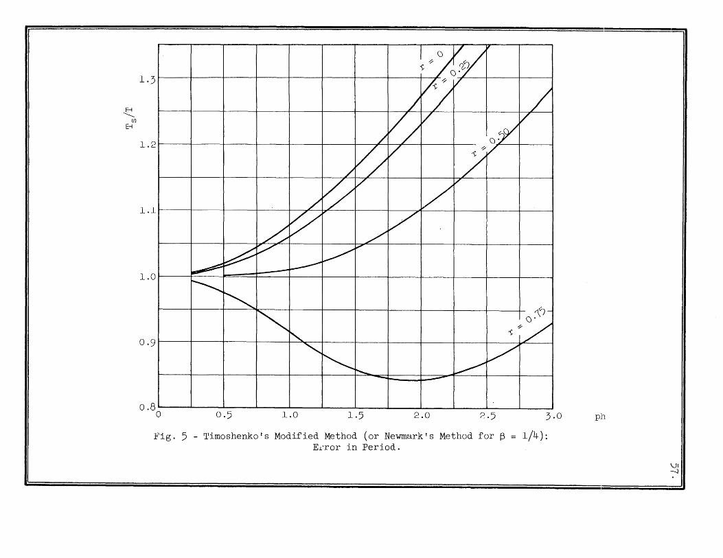
E-I -..... [f)
E-i
1·3
1.2
1.1
1.0
0·9
0.8 o
~ ~
~
""
0·5
/
~ ~ y
L----'"'
~ "-
"" 1.0
I () ~ ~ 'l 'l-~ o·
Y7 / v/ v v
/ or ~ V 'l
/ /
'i v v v
./ :/
~ ~
~~-o·
~'l/
~ / ~ ~
-t--. -1·5 2.0 2·5 3·0
Fig. 5 - Timoshenko's Modified Method (or Newmark's Method for ~ = 1/4): E1.TOr in Period.
pJh
\Jl --.:]

~ (f)
.~
V 1.5LI--~--~---+---+--~---j--~
I /J Envelope of amplitude '?}O/--
t- ----- at pt = 1 0;)1"
/ -\-y 1.41--- --- Peak amplitud: in first "'()~
cycle due to Yo = p. / ~
I I
1·3 rl-IT-r-+--f1~+~~~~--l~
1.2
/ / ~
1.1
1.0 I I ~ I I I I I r~=o21 o 0·5 1.0 1·5 2.0 2·5 3·0
Fig. 6 - Timoshenko's Modified Method (or Newmark's Method for ~ 1/4): Error in Amplitude.
ph
\Jl CD
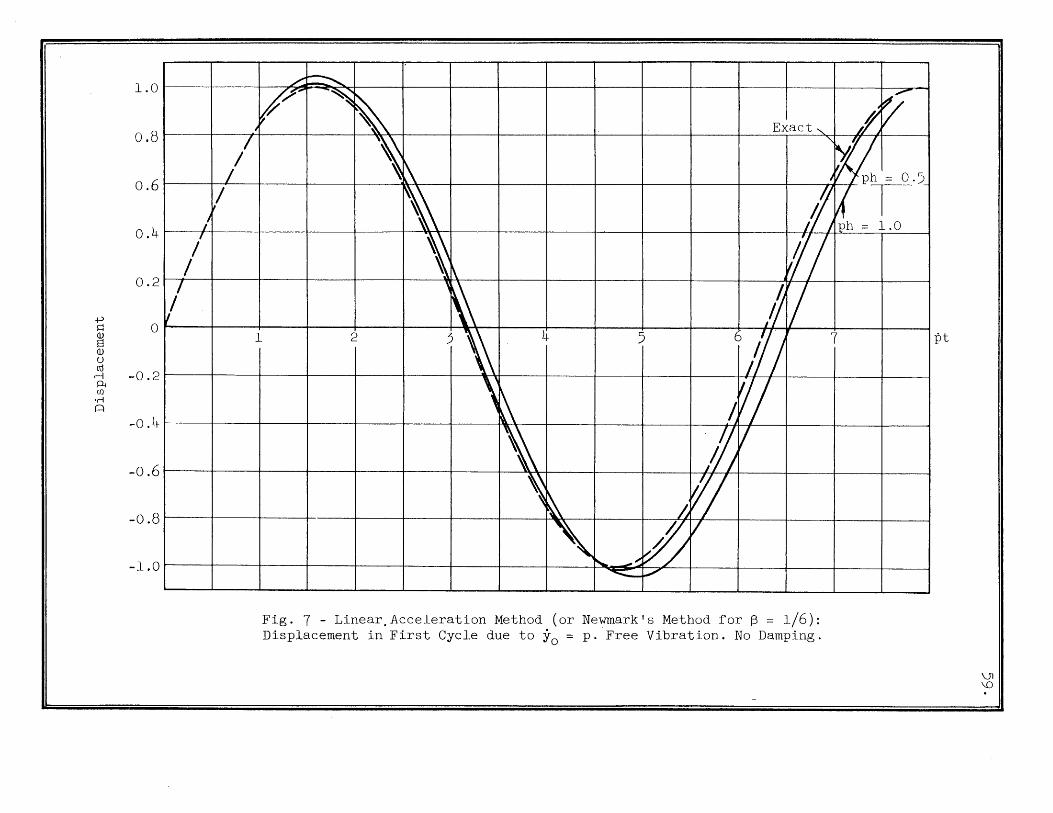
-f-J
Q Q)
S Q) ()
cd r-I P-l (f)
'M ~
1.0
0.8
0.6
0.4
0.2
0
·-0.2
-0.4
-0.6
-0.8
-1.0
Fig. 7 - Linear,Acceleration Method (or Newmark's Method for ~ = 1/6): Displacement in First Cycle due to Yo = p. Free Vibration. No Damping.
pt
\Jl \0

I I I Stability Criterion
1.2 -
r ph 0 3.46410 E-I
-............ [j)
r-- 0.25 3.35410 E-I 0·50 3·00000
0.75 ?29129 1.1 '---
./
~ ~ ---~ ~ -------~ r----
1.0
"" ~ '" 0·9
0.8
0·7 0 0·5 1.0
I r = 0
~ ----- 1\1 / '/ r = 0.25 \ ~/ ~ ~ ~ .-- 1\
/ ~ ~ \ / ~ I
~ 1 I
I
I r-------- I
1:' - 0
-~ I
~
I\. \ '\
, I
I\~ ~
I
- ------- I
1·5 2.0 2·5 3·0 3.5 ph
Fig. 8 - Linear Acceleration Method (or Newmark's Method for ~ 1/6): Error in Period.
0\ o

1·3
1.2
~ 1.1 (f)
~
1.0
0·9
0.8
I I I I ~ Convergence Criterion
r ph I---
0 2.44949 0.25 1.81174
_ 0·50 1·37228 0·75 1.07603
//'
// ./
~~ '/ ./
/' P ,~ y V~ V,..... ..
/' ~
~ ~ ~
~ ------ r-- __ . ~ ---........ " .......
1' ......... .r ,~
",-0'/5 ,~
" ", , o 0·5 1.0 1·5
I I / I Q<r;l,1 J I
J /r" 0°, af l' 11
/" 117 Ay / ~/" Y all I I V'
/1 /
1/</ V ().
;'/ ~~ --; V //
I- ~~ V ",," ~ ~ / ~ /" Stability Limit/
~
? V- I
Envelope of amplitude at pt = 1. (Effect of initial condi-tion neglected. Magnification factor taken as unity).
--- Peak amplitude in first cycle due to Yo = p.
\ 2.0 2·5 3·0 3 t:"
.)
Fig. 9 - Linear Acceleration Method (or Newmark's Method for ~ 1/6): Error in Amplitude.
ph
0\ r-'

C\J 1.2
\.0
1.0
0.8
0.6
0.4 / /'
0.2 +J ~
~ 0 Q)
" / /
I
u ro r-l PI U) -0.2 'r!
c::l
-0.4
-0.6
-0.8
-1.0
I ~ ph = 1.0 12':...--/' ~
ph = O.t ~' y.' -" ~ if/ "
~
/' ~~ J/' ~,
Ii JI ~ Exact _ t\
I' ~\ \ I \ 1 ~ /
6 I 7 1 2 3\ 4 5
19
\ / ~ l.
1\ h ~ LI \, ~~
)(1
I' ~ .~ f rI ~~ V
Fig. 10 - Parabolic Acceleration Method: Displacement in the First Cycle due to Yo = p. Free Vibration. No Damping.
pt

8 -............
rJ)
8
1.4 _.
1·3 I
) 1.2
1.1
1.0 o
r - 0
~ ~ ~
r\ V !--.. VV
Parabolic 1
~ ~inear-parabolic ~--~---- I I I 0·5 1.0 1·5 2.0 2·5 3·0
Fig. 11 - Parabolic Acceleration Method: Error in ~eriod
I
I 1
I
I
3·5 ph
0\ \..)J
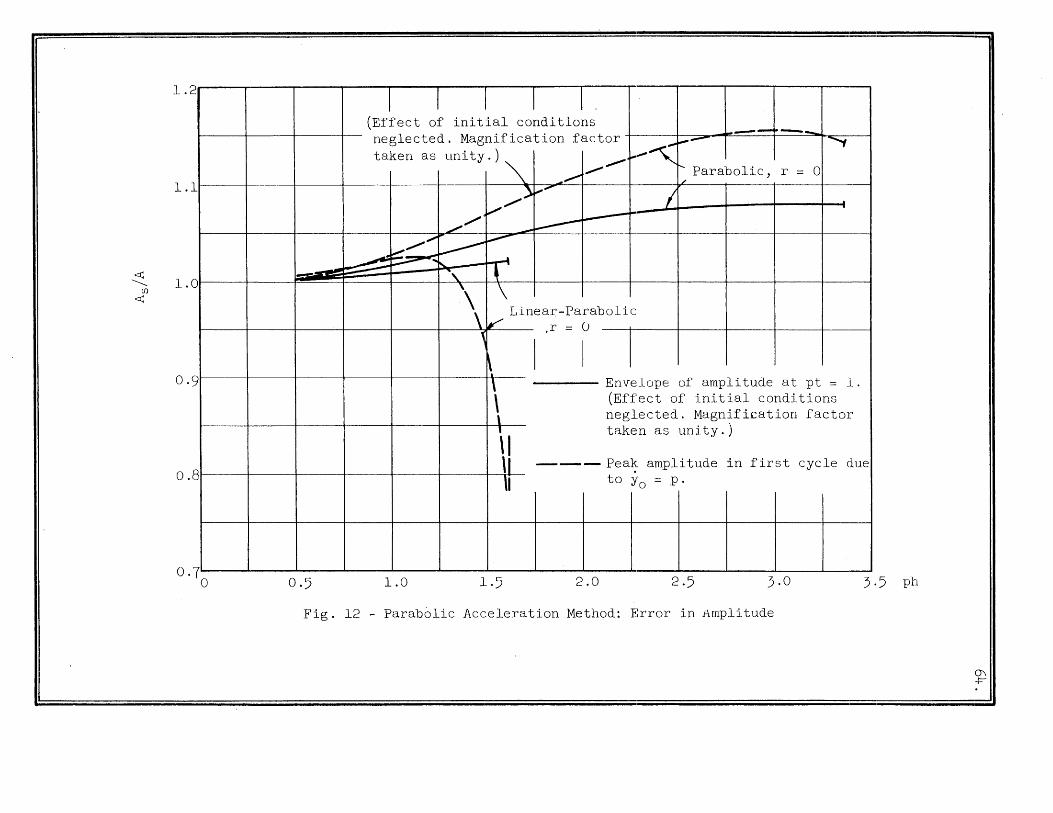
1.2
1.1
~ 1.0 ({)
<r:
0·9
: 0.8
0·7 o
I I I I I , (Effect of initial conditions ---.. --neglected. Magnification factor
~~" 1-- ""1
taken as unity.) "\ .,.,,~ ~ Parabolic) r = 0
_/ /
,.....) ~ .... I ~
-.
/' ~ ~ ..", -"..-""'" ~
~
-~ ~r:. -" - -, , '\ \
\ Linear-Parabolic
V .r = () ~
I I ~, 1 Envelope of amplitude at pt = 1.
\ (Effect of initial conditions
\ neglected. Magnification factor
\1 taken as unity.)
\I --- Peak amplitude in first cycle due
11 to ~o = p. -
I I I I I I I
0·5 1.0 1·5 2.0 2·5 3·0 3.5 ph
Fig. 12 - Parabolic Acceleration Method: Error in Amplitude
0\ +

(\/ 1. ;:F: Q...
,---...",. c:o.. I
1.8
1.
I 1 I I C\J \ I Jf .-I
Stability Criterion 0 -- ~J .-I II if j II
~ ph en. en.
7 1/4 00 i/ 1/6 3.46410 1/8 2.82843 I I 1/12 2.44949 I ~ I 0 2.00000
6 J J
/ / ! -~ r -
1.
~ +"' .r-! U 0 .-I (1)
> I-! 1. 0
ct-!
I-! 0 +"' u C\l ~
C 0 1. .r-!
+"' C\l U
.r-! ct-! 'r! C bD C\l ~
1.
/ I / / 5
I I I II I / / - /
4 l
I / / I V
3 I[ Y J If I J
/ / / I V
2
/ ) VI I ~/ / I/' V V
1 ~
~ ~ V / 1.
~ ~ ~
.A ~ :: 1/4
0 -- I' I 1.
2.0 o 1.0 ph
Fig. 13 - Newmark's ~-Method: Magnification Factor for Velocity

E-t ...............
r.n
1.2
E-t 1.1
1.0
0.8
0.6
66.
I I I Stability Criterion ___
r ph If\ r:- -0 0 2.00000
II 0.25 1·93649 ~ 0·50 1·73205 _
0·75 1·32288
~ _"'lI ~~
~ ~,
~ ~ ~
~ .'\ ~ ~
1\ \\ ~~ \~ \
\\
~ 0
~\\
~o \~\ 0-
\ \ \ \ '
\ 0·5 1.0 1·5 2.0 2.5 ph
Fig. 14 - Levy's Method (or Newmark's Method for ~ = 0): Error in Period
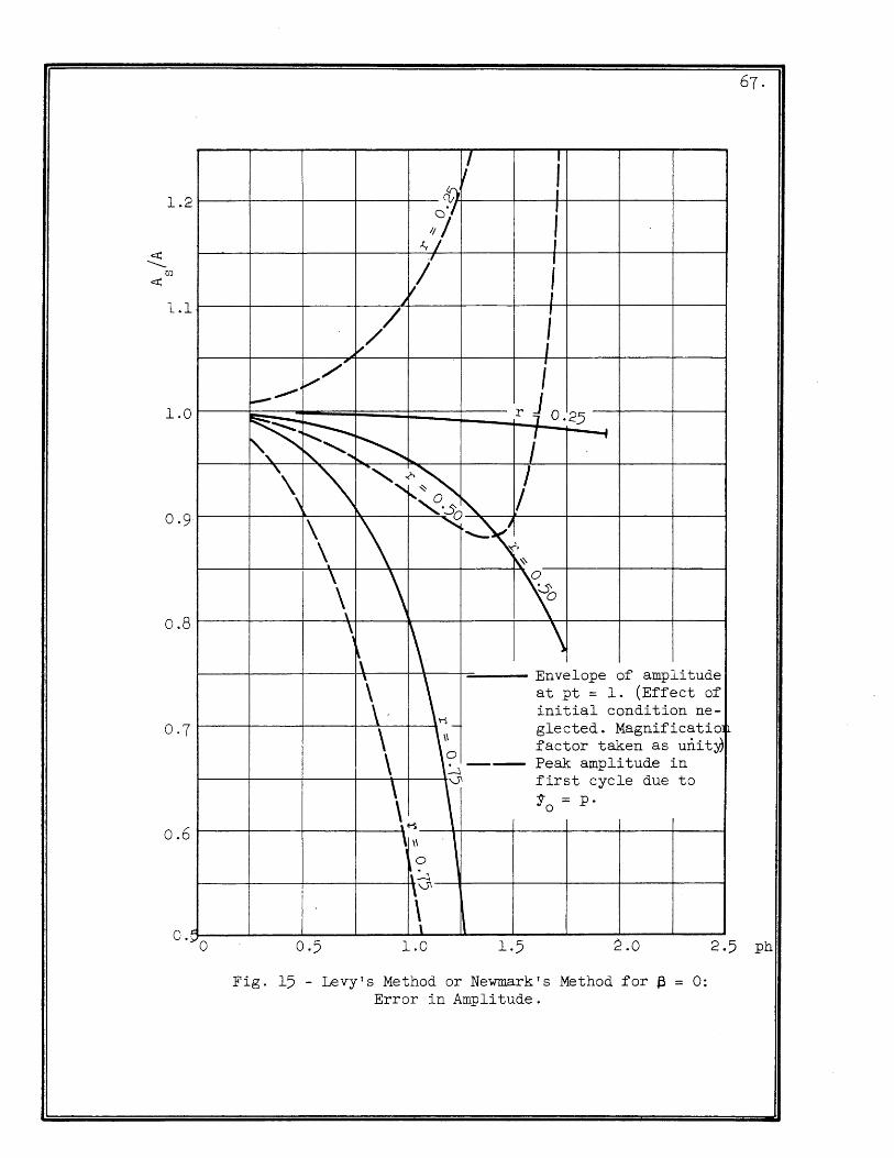
/ i ct. I
~I I II
ty/ I
1.2
/ , / ! j
/ i ~/ I
1.1
/' i ~"".",
V
r _1 0.25 ~
~ ~ ~ / ---t
" ~ '-"
1.0
'\ '\ -, <-.~ I -, ~
\ ~ '~·..5'O' / \ \ '-"<, \~ ~
0.8
\ \ , \ \
\ \ \ \ Envelope of amplitude
\ \ at pt = 1. (Effect of
\ ' K_ initial condition ne-glected. Magnificatio~
\ \: factor taken as unit~ \ ~--- Peak amplitude in
\ \ first cycle due to -S ;:: p.
\~ 0 , \\ \ 0
1~ \V \ \ r:: \
).
0.6
o. 2.0 1·5 2.5 ph o 1.0
Fig. 15 - Levy1s Method or Newmark1s Method for ~ = 0: Error in Amplitude.

68.
l. 0
~ r-----r---.. --~ ~ ~ '- ~~
~ ~ ""' ~::'\ ~. ~."5 ~
9
'\ ~ '\ \ \C
o.
~~ ~ , \
·so ~ 8
\ \ \ . 0
~Stability Criterion ~ .....5'
\ \ I ph r
o.
7-~
0 2.44949 \ 1\ 0.25 2·37171 _ 0·50 2.12132
0·75 1.62018 1 \ I'" U 1
o.
o.
o. 5
o. 4
1.0 2.0 2.5 ph
Fig. 16 - Newmark's ~-Method for ~ = 1/12 and Sa1vadori's Method: Error in Period
\1 II
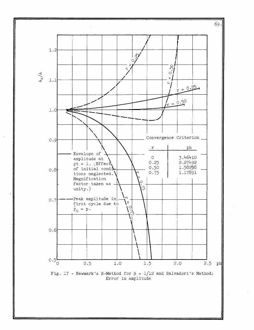
~I ~ /' ,
I !CI al I /; o. jl :;;1
1.2
~ / "I V ~/
~Cf) 1.1
/~ 0.2') ./ I ~
,// ~ l.----" iLJ·50 ----.---'
, L.-----~ -~
~ ,
F-::::: --1----- II
~" ~ !'------- -"",/
"
1.0
r-'\. ~ \ Convergence Criterion _
\ \
0.8
I ~\ -- Envelope of ~\
amplitude at ~ \ pt = 1. ~Effec;\ ~ I- of initial cond ~ tions neglected.\ ~o Magnification A
f- factor taken as unity.) \ r I---Peak amplitude in ,--i ~irst cycle due to \\ \ Yo = p. \C?~
~
0.6
0·5 o
\
1.0
, \
\
\ \
\
\
r ph
-0 3·46410
0.25 2.27492 0·50 1.58258 -0·75 1.17891
\ 2.0
Fig. 17 - Newmark's ~-Method for ~ = 1/12 and Salvadori's Method: Error in Amplitude

1.2
1.0
0.8
0.6
0.4 I /
4J sj Q) 0.2 s Q)
II /
u ill rl ~ 0
! U)
'rl ~
-0.2
-0.4
-0.6
-0.8
-1.0
v-~ ~ ~
" '" ~- ", ~~ .~
/~
// .1
/' \ \ \ /' \ Exact -..... L 1- , j
,/ \,\ \ / V ~ 1 i
'\ 1\ \ / Ah = 0.5 \ l
\\ \ i V
I / ~
1 2 3 '\ ' 4\ 5 6 /' /7 / \ ~ ,I \ ~\ \
'" V
/ V ,
r\ / J '\ \ \ /' / /
~h b_ 1.0 \. \ I \,
-~\ .~ tJ V / "' /
'\. ~ // V ' ... L-/ ~ .""
Fig. 18 - Houbolt's Method - Displacement in First Cycle due to Yo p. Free Vibration. No Damping.
pt
---J o
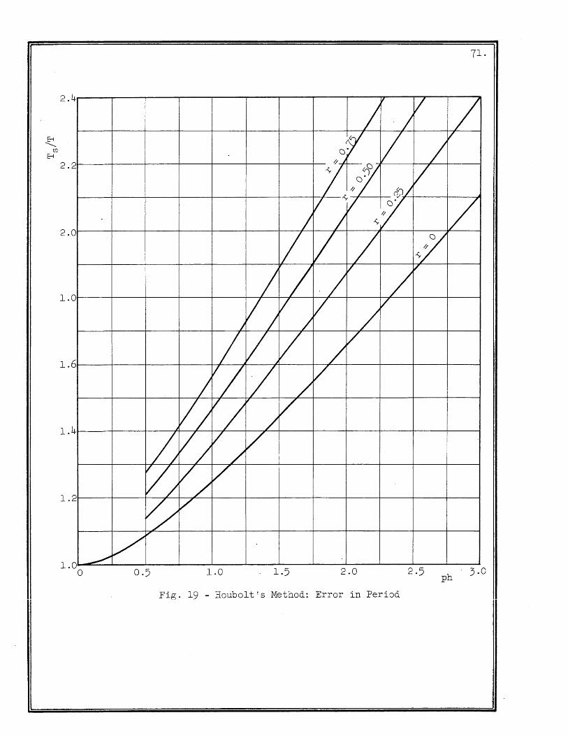
2.4
2.2
2.0
1.0
1.6
1.4
1.2
1.0 o .-/
71.
'I V / / .j
qat V /
/ I.f V
/fa' hI
V ~v 1 !/ I j ,(,,/f
/ V / ~y
/ V / V /' jV / 1 7 /
/
/
/ V V / /
I VI / / V
,VI // " / /
/; v/ / V /
I> // / 'i V
v~
1.0 . 1.5 2.0 2·5 ' 3·0 ph
Fig. 19 - Houbolt's Method: Error in Period

E--t ~
U)
2 ~
. c
E--t 2 .c
c: .c 1
I' .L-1
1. I
r '-1.
/ 1. c
"-
00 u \
o.
~
c o.
/ /
/
/ V
~
\ "
72.
)j / / 1 v
/ II
/ ~I 1 I II
I / ~I
/ / v / / /
/
/ I V / / v K1 oJ J II .
/ j' 'I "/ / J
/ I / V 'I V / / )
/ V / /
/ 7 v /
V V /
v / /'
v /
~ V
o 1 2 3 4 5 (}Ph
Fig. 21. - Eu1er l s Method: Error in Period

r-l
II
+=' Pi
1.8
1.6
1.4
1·3
+=' 1.8 m
~ .£ 1.1
1.0
0.8
1 :1-~
73·
l----'-~J5---
-~
~
V ./
/ V
/~ I/' r - O.'5Q_
/ ~ ~ -----V ~ ~ ~ V
r := 0.25
~ ~
----r----~ r - 0
1.0 2.0 2·5
Fog. 20 - Houbolt's Method: Error in Amplitude

74.
2 "... .\,..; l/;r V
tr\~
0 T' 1/ l' tr\
.4 /-.i t-•
\ f.I
~/ tr\ ~. t-
o 1.,
/ " • v--- --r-----. r----.~ = 0 ·50 ~\ / 17'
C.
~ VI V
2
2.
0 ~ I !f 01,
/1 0 " 1/ -If
HI/ ~
\ il ~ l 0) f/ t; ./
""".-- ---~ u "JD , V ---------.: = 0.25 -
r-----.r----. J I /
2.
L n IVV u 1 f1 1.
I
t/ ~ ---r-----.
l r----. ------1 /1 ------ r ::: 0
"t"
'. //1/ ~~ --Envelope amplitude at pt = 1. _
Jr ---- Peak amplitude in first cycle
1.
~ due to Yo = P f" • c:. -1.
V 4
1. n o 1 2 3 4 5 ph
Fig. 22. - Euler's Method - Error in Amplitude
II II

I I I r II' I
1.8
L.(\ / t-
o IV . II
H
QO/ / ,(,. V
~v / V 00/ j
1.6
I / 1 I /
IT / I /
1.4
V / V () / J J / ()~
7 V V ~
{.-
/
1.2
/ V / / /
/ ~
~ V~ /' V /
1.0
~ / / / '\~/ ~ /
\'-~ ,/ / ~
/ ./
0.8
V / V
/ \ V ,v v-
"---"""
0.6
o 1 2 3 4 5 ph
Fig. 23 - Modified Euler Method: Error in Period

76.
2.
IIi' ~ /' ~ ~
0 II :;: l!) '.r~O / II 1/ 1/
HI H
t'l/l / 8
Jf 1/ 1.
II V V ~ - r---~o
6 r---.. II 11/ J Ii
1.
~ (J)
~. 1.
I /1 'I
4 /,l r = 01050TTV
'J - r
l = 002
5,11/), ~r- r = O)V It I 1.
7J Ill/I Envelope of amplitude at
~ ~/ pt = 1. (, /~ ...,
-~ ,
1 -
:~'-/J -------- Peak amplitude at first
cycle due to Yo = o.
1.
\\ ./ a \\ o.
\ ~ r = 0.7;1\ \ ~
t2.. ....,
\\ o.
o 1 '3 4 5 ph
Fig. 24 - Modified Euler Method: Error in Amplitude

77·
2. 0 I I o 11\ 11\ t--
0 0
II-II
?-i ?-i
1. 8
I
6 I I
1.
I, I I /
I Y );
1.
I / / r- / L.
II / 07 /
/~ ,V V 0
~r-...... ./
'~ V / 1\ ./
1.
1.
, K / ~/ / 8
\~ "---"""' v
/ /
O.
\ / /'
6 \
~ V -o.
o 1 2 3 4 5 ph
Fig. 25 - Runge) Heun and Kuttats Third Order Rule: Error in Period
II II

2.
2.
1.
1.
1.
1.
1.
O.
O.
78.
c:.
! /j J
/I f T V :H"r = 0 .25
f' 1/) = 0/
l I7~' JJ TV ~ ~-~~I '/ I 1/ I , A.., • J
. / I / .!o~ I II ~ r = 0 e -<;. - -If I ' 1/
~
j ! I / ,- !J
~ '/ / I 1/ /
\...
1/ ."/ / / II '/ V \ J~
VI ffl I 1/ ~
Y r r = 0.75 I I • t:
//~ ~ I N '/ / 1/ Envelope of amplitude at ~
Il' pt = 1
( r = 0 ~ --- Peak amplitude in first cyclE
~l k' n due to Yo = p.
~~ J
_\ [VI ( / I... r - 0.25 \, \71 I~ ../) -r = 0.50 -J I
0 I \
1 2 3 4 5
Fig. 26 - Runge, Heun and Kutta's Third Order Rule Error in amplitude
p h
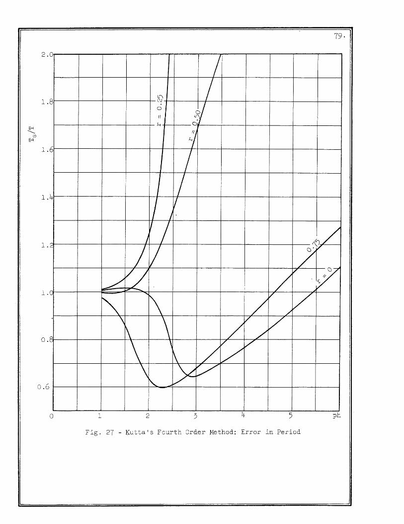
II
2.
1.
"1 ..1...
1.
1.
1.
o.
0.6
0
8
6
4
c:::.
C
0 '---
o
79·
lI\ / C\J
# 0
1/
H
1 7
I / I /
/
I ~/ I
/ V v/~ ~ V/ / ~ ..." ..........
"" '\ / V V
/ \
/ V /
~ ./
\ \ V V ~ / V
\ LY / '- .,
1 2 3 4 5 ph
Fig. 27 - Kutta's Fourth Order Method: Error in Period
II

80.
2.2 I I J I _i i7~ r = 0.75 I ~. !
Ii
I 1 t! II r = 0.50
I /' I V II ~o~ jJ
I r il If / ~
I J /! I I / /~
I
2.0
1.8
I i / II v I
I I V i / i '/ J
I i 11/ 11 V r =,0.25
I r = 0
1.6
/ If ~' f i -' ~ J ! J ~IJ
/;1/ /1/ Envelope in amplitude at
III pt = 1
1.2
L ~J ~ -------- Peak amplitude in first
cycle due to y = p. 0
~ .,,,~
~ II ~~
'J 0,,-
~ 1.0
'\, I
~ I \ , ',\'-~ i \~
I
0.8
\ I \ I
\ I 0.6 o 1 2 4 5 6p
Fig. 28 - Kutta's Fourth Order Method: Error in Amplitude

100
10
/~ I~ h 'I '/
1.0
l~ ~ ............
~, ."'" ..... W .\. "'-~\\ \ \\\ \
\\
\ 0.1
0.01 o I o
I 1/ I I / / / / / ?Itt I I C? .. 0{ / /
CV "i "7: '-;f-"'- -v- / / I / / / / v / / ill
II; Ijl 1 II I I / I II I / /
I III / if II I / / / 111/ V /
IJI// / Y/j / / // V
/ ~ .........
.............
""- ~
'" ............
\ ,,~
\\ ~ \\\ 1\
\ \ \. \ \ \ \. \ \ \ \ \ \ \ \ \ \ \ \ \ \ \ ~ \
~~\ 5
1
If I J "i/ v / / / Y
v / j J 1/ /
/ /
1/ V / /
/ / / ./
/ /' V
/' ./
/ .. J../" ,.... V"
~ ~
r-.....
"" ............ ~ '" ~ ~
'-'-
" \ " \ " \ '" \ " '" r\ ~ , ~ 10 I .
15 I I 2
81.
I /'
ev,/' "/
/' /
/ ./'
">-Y ./ ~
..",
.L" .."",
./ ,..."
AsiA atpt = 1.0--;
~ "" ......... .........
..............
1\ '" 2b
3
...........
25 I
4
~ ~ ...............
..........
30pt
cycles
Fig. 29 - Values of AsiA at Any Stage for Various Values of AsiA atpt = 1.

1.2 1
'\ Houbolt's region of
~ laperiodic \ response
/. \ \~
.......,.;.
r---\ ~ ~ ~ ~ ~
r
1.0
'" 0.8
o~ 'M (f)
rd s:J o 0 'M H (f)
ill ill P-iP::; 0.6
0.4
0.2 :
o
L ~ 'M rd s:J o 0 'M H (f)
ill ill PIP::; ~ Exactr-J
[ (TimOShenkO' S Method or Newmark's j3 = 1/4 }
~ r-,,- ~ Methods of Euler, Modified Euler, Runge, ~ t Heun and Kutta
~ O'<\' ~~ -
I'~Q<t ~ ~
\~ '" ~ ~ I
\ I' ~ 1
\ ~ (»(>.f><\,c •
\ '0 ~ " ~ ~ '... ~Ci , ~~~ \ 1\.f>+B ~
" Vo ., ~
~~ ~\~o \ ~ ~~ ~ \~\ \ Q~'f~ \ , ~ \ ~~,~ \
'-- ... 1"'",-
............ "-
-----.......... ~
1 2 3 ph
Fig. 30 - Criteria for Critical Damping CD f\)
a.
DISTRIBUTION LIST - PROJECT NR 064-183
Administrative, Reference and Liaison Activities
Chief of Naval Research Department of the Navy Washington 25, D. C. ATTN: Code 438 (2)
Code 432 (1)
Director, Naval Research Laboratory Washington 25, D. C. ATTN: Tech. Info. Officer (9)
Technical Library (1) Mechanics Division (2)
Commanding Officer Office of Naval 'Research Branch Office 495 Summer Street Boston 10, Massachusetts (1)
Commanding Officer Office of Naval Research Branch Office 346 Broadway New York City 13, New York
Office of Naval Research The John Crerar Library Bldg. Tenth Floor, 86 East Randolph St. Chicago 1, Illinois
Commander U.S. Naval Ordnance Test Station Inyokern, China Lake, Cal~ornia ATTN: Code 501
Commander U. S. Naval Proving Grounds Dahlgren, Virginia
(1)
(2)
(1)
(1)
Commanding Officer Office of Naval Research Branc.g Off ice 801 Donahue Street San Francisco 24, California (1)
Commanding Officer Office of Naval Research Branch Off ice 1030 Green Street Pasadena, California (1)
Contract Administrator, SE Area Office of Naval Research Department of the Navy Washington 25, D. C. ATTN: R. F. Lynch (1)
Of~i£er in Charge Office of Naval Research Branch Office, London Navy No. lOO FPO, New York City, New York
Bib~ary of Congress Washington 25, D. C. ATTN: Navy Research Section
Commander
(2)
U. S. Naval Ordnance Test Statio~ Pasadena Annex 3202 East Foothill Blvd. Pasadena 8, California ATTN: Code p8087 (1)

Department of Defense Other Interested Government Activities GENERAL
Research and Development Board Department of Defense Pentagon Building Washington 25, D. C. ATTN: Library (Code 3D-I075) (1)
Armed Forces Special Weapons Project P.O. Box 2610 Washingtop.., D. C. AT~J: Lt. Col. G. F. Blunda (1)
Joint Task Force 3 12 St. and c~t. Ave., N.W. (Temp .U) Washington 25, D. C. ATTN: Major B. D. Jones (1)
Chief of Sta.:ff Department of the Army Research and Development Division Washington 25, D. C. ATTN: Chief of Res. and Dev.
Office of the Chief of Engineers Assistant Chief for Public Works Department of the Army Bl.dg. T-7 , Gravelly Point Washington 25, D. C. ATTN: Structural Branch
(R. L. Bloor)
O~fice of the Chief of Engineers Asst. Chief for Military Const. Department of the Army Bldg. T-7, Gravelly Point Washington 25, D. C.
(1)
(1)
ATTN: Structures Branch (1) (H. F. Cdrey) Protective Construction Branch (I. b. Thorley) \ (1)
Office of the Chief of Engineers Asst. Chief for Military Operations Department of the Army Bldg. T-7, Gravelly Point Washington 25, D. C. ATTN: Structures Dev. Brch (W.F. Woollard) (1)
Engineering Research and Development Laboratory Fort Belvoir, Virginia ATTN: Structures Branch
The Commanding General Sandia Base, P.O. Box 5100 Albuquerque, New Mexico ATTN: Col. Canterbury
Operation Research Officer Department of the Army Ft. Lesley J. McNair Washington 25, D. Co ATTN: Howard Brackney
(1)
(1)
(1)
Office of Chief of Ordnance Research and Development Service Department of the Army The Pentagon Washington 25, D. C. ATTN: ORDTB (2)
Ballistic Research Laborat9TY Aberdeen Proving Ground Aberdeen, Maryland ATTN: Dr. C. W. Lampson (1)
Commanding Officer Watertown Arsenal Watertown, Massachusetts ATTN: Laboratory Division (1)
Commanding Officer Frankford Arsenal Philadelphia, Pa. ATTN: Laboratory Division (1)
Commanding Officer Squier Signal Laboratory Fort Monmoutn, New Jersey ATTN: Components and Materials
Branch (1)

Other Interested Government Activities
Chief of' Bureau of Ships Na-TY Department Washi,ngto::J. 2]5 ~ Doe 0
AT~~~ Director of Research Code 4~,o \-::;od.e )+30 Code 421
DirectoT J
:;)avid Taylor Model Basin Washington 7J Do C. ATTN~ St::.-uctural Mechanics
Division
Di.:rector'J Naval Engro Experiment Station Ar.',rlapolis 2 Maryland
Director Materials La~oratory New York Naval Shipyard :Brooklyn 1, New York
Chief of Bureau of Ordnance Nav-Y' Department Washington 25 7 Do C. ATTN~ Ad·~3J Technical Library
Reeo) P. Eo Girouard
Superintendent, Naval-Gun Fa~toTY Washington 25, Do Co
Naval Or~nance Laboratory Whi,te Oak:.? Maryland RED 1" Silver Spring, Maryland AT~J~ Mechanics Division
Naval Ordnan:e Test Station ILyokern~ California AT.TN~ Scientific Officer
Naval Ord.nance Test Station Underwater Ord...-rJ.an::e Division Pasadena 2 California ATTN~ structures Division
Physics Division
(2) (1) (1) (1)
(2)
(1)
(1)
(1) (1)
(1)
( ~\ -)
(1)
(1)
Chief of Bureau of Aeronautics Navy Department Washington 25, D. C.
c.
ATTN~ TD-41; Technical Library (1) DE-22, c. W. Hurley (1) DE-23; E. M. Ryan (1)
Naval Air Experimental Station Naval Air Material Center Naval Base Philadelphia 12, Fa. ATTN~ Head, Aeronautical Materials
Laboratory (1)
Chief of Bureau of Yards and Docks Navy Department Washington 25, D. C. ATTN~ Code P-314 (1)
Code C-313 (1)
Offiser in Charge Naval Civil Engro Research and Evalo Lab, Naval Station
Port Hueneme, California (1)
Superintendent Pest Graduate School Do So Navay Academy Mo~terey, California (1)
AIR FORCES Commanding General Uo s. Air Forces The Pentagon Washington 25, D. Co AT~!~ Research and Development
Division (1)
Commanding General Air Material Command Wright-Patterson Air Force Base Dayton., Ohio ATTN: MCREX-B (E. H. Schwartz) (2)
Office of Air Research Wright-Patterson Air Force Base D ayt or. :; Ohio ATTN~ Chief, Applied Mechanics
Group (1)

OTHER GOVERNMENT AGENCIES
U. S. Atomic Energy Commission Division of Research Washington, D. C.
Argonne National Laboratory P. 0. Box 5207 Chicago 80, Illinois
Director, National Bureau of Standards Washington, D. C. ATTN: Dr. W. H 0 Ramberg
U. S. Coast Guard 1300 E Street, NoWo Washington, D. C. ATTN: Chier, Testing and
Development DiVision
Forest Products Laboratory Madison, Wisconsin ATTN: L J 0 Markwardt
(1)
(1)
(2)
(1)
(1)
d.
National Advisory Committee for Aeronautics
1724 F Street, N.W. Washington, D. c. (1) "
National Advisory Committee for Aeronautics
Langley Field, Virginia ATTN~ Mr. E. Lund~uist (1)
National Advisory Committee for Aeronautics
Cleveland Municipal Airport Cleveland, Ohio ATTN: Jo H. Collins, Jro (1)
U. S. Maritime Commission Technical Bureau Washington, Do C. ATTN: Mr. V. Russo (1)
CONTRACTORS AND OTHER INVESTIGATORS ACTIVELY ENGAGED IN RELATED RESEARCH
Professor Jesse Ormendroyd University of Michigan Ann Arbor, Michigan
Dr. N. J. Hoff, Head TIepartment of Aeronautical
Engineering and Applied Mechanics Polytechnic Institute of Brooklyn 99 Livingston Street Brooklyn 2, New York
Dr. J. N. Goodier School of Engineeringr .. Stanrord" University Stanfor~, California
Professor F.o K. Teichmann Department of Aeronautical Engr. New York University University Heights, Bronx New York City, New York
Professor C. T. Wang Department of Aeronautical Engr= New York University University Heights, Bronx New York City, New York
(1)
( 1)
(1)
(1)
(1)
Professor M. A. Sadowsky Illinois Institute of Technology Technology Center Chicago 16, Illinois (1)
Dr. Wo Osgood Armour Research Institute Technology Center Chicago, Illinois
Professor R. L. Bisplinghoff Massachusetts Inst. of Tech. Cambridge 39, Massachusetts
Professor Bo Fried Washington State College Pullman, Washington
Professor E. Reissner Department of Mathematics Massachusetts Inst. of Tech. Cambridge 39, Massachusetts
Dr. A. Phillips School of Engineering Stanford University Stanford, California
(1)
(1)
(1)
(1)
(1)
e.
CONTRACTORS AND OTHER INVESTIGATORS ACTIVELY ENGAGED IN RELATED RESEARCH
Professor E. Sternberg Illinois Institute of Technology Technology Center Chicago 16, Illinois
Dr. W. Prager Grad. Div. Applied Mathematics Brown University Providence, Rhode Island
Dr. W. H. Hoppmann Department of Applied Mechanics Johns Hopkins University Baltimore, Maryland
Professor W. K. Krefe1d College of Engineering Columbia University New York City, New York
~rofessor R. M. Hermes University of SantaC1ara Santa Clara, California
Dr. R. P. Petersen Director, Applied Phyqics Div. Sandia Laboratory A1ou~uerque, New Mexico
Dr. R. J. Hansen Massachusetts Inst. of Technology Cambridge 39, Massachusetts
Dr. Francis H. Clauser Chairman, Dept. of Aeronautics The Johns Hopkins University School of Engineering ~altimore, 18, Maryland
Dr. G. E. Uhlenbeck Engineering Research Institute University of Michigan Ann Arbor, Michigan
Dr. Walter Bleakney Department of Physics Princeton University Princeton, New Jersey
(1)
(1)
(1)
(1)
(1)
(1)
(1)
(1)
(1)
(1)
Professor L. S. Jacobsen Stanford University Stanford, California
Professor A. C. Eringen
(1)
Illinois Institute of Technology Technology Center Chicago 16, Illinois
Professor B. J. Lazan Engineering Experiment Station University of Minnesota
(1)
Minneapolis 14, Minnesota (1)
Professor Paul Lieber Dept. of Aeronautical Engineering
and Applied Mechanics Polytechnic Inst. of Brooklyn 85 Livingston Street Brooklyn 2, New York (1)
Professor Vito Salerno Dept. of Aeronautical Engineering
and Applied Mechanics Polytechnic Insto of Brooklyn 85 Livingston Street Brooklyn 2, New York (1)
Professor George Lee U.S. Naval Post Graduate School Annapolis, Maryland (1)
Professor L~oyd Donnell Department of Mechanics Illinois Institute of Technology Technology Center Chicago 16, Illinois
Professor Lynn Beedle Fritz Engineering Laboratory Lehigh University Bethlehem, Pennsylvania
Dro Bruce Johnston 301 West Engineering Bldg. University of Michigan Ann Arbor, Michigan
(1)
(1)
(1)

Library, Engineering Foundation 29 West 39th Street New York City, New York
Professor N. M. Newmark Department of Civil Engineering University of Illinois Urbana, Illinois
Dean W~ L. Everitt College of Engineering University of Illinois Urbana, Iilinois
Professor T. J. Dolan Dept. of Theoretical and Applied
Mechanics University of Illinois Urbana, Illinois
(1)
(2)
(1)
(2)
TASK VI PROJECT - C. E. RESEARCH STAFF
W. H. Munse
G. K. Sinnamon
R. J. Mosborg
H. C. Roberts
W. J. Austin
-L. E. Goodman
c. P. Siess
Research Assistants
Files
Reserve
(10)
(5 )
(20)
Dr. C. B. Smith Department of Mathematics
f.
Wdlker Hall, University of Florida Gainesville, Florida (1)
Dean R. E. Johnson Graduate Coililege University of Illinois Urbana, Illinois (1)
Professor W. C. Huntington, Head Department of Civil Engineering University of Illinois Urbana, Illinois (1)
Erofessor A. E. Green Kings College Newcastle on Tyne, 1 England
Dr. L. Fox Mathematics Division National Physical Laboratory Teddington, Middlesex England
Professor Wo J. Duncan, Head Dept. of Aerodynamics College of Aeronautics Cranfield, Bletchley Bucks, England
Professor R. V. Southwell Imperial College of Science
and Technology Prince Consort Road South Ken~ington London S.W. 7, England
(1)
(1)
(1)
(1)