a comparison of mjo indices for the dynamo field campaign · a comparison of mjo indices for the...

A Comparison of MJO Indices for the

DYNAMO Field Campaign

George N. Kiladis

Physical Sciences Division

Earth System Research Laboratory

NOAA

work in collaboration with:

Juliana Dias

National Research Council Postdoctoral Fellow, NOAA/ESRL

Katherine Straub

Susquehanna University, Susquehanna Pennsylvania

Stefan Tulich

CIRES, University of Colorado, Boulder

Goals of this study:

Define an satellite-only (convective) based index of the MJO

Compare this new index with others already in use

Assess the utility of each index for both statistical analysis and real-time monitoring of the MJO

Do we really need yet another MJO index?


Lau and Chan (1985); Ferranti et al. (1990); Zhang and Hendon (1997); Maloney and Hartmann (1998); Higgins and Shi (2001); EOFs of time-filtered filtered OLR

von Storch and Xu (1990) POP analysis of 200 hPa Velocity Potential from 45S-45N

Waliser et al. (1999) SVD of 30-70 day filtered pentad OLR from 30S-30N

Lo and Hendon (1999) EOFs of spectrally truncated (T12) OLR and 200 hPa streamfunction

RMM (Wheeler and Hendon 2004)-combined EOF of OLR, u850 and u200 averaged from 15S-15N, with 120 day running average and ENSO removed

Kikuchi and Wang (2012) OLR EEOFs (Extended in time)

CPC- EEOF of 200 hPa Velocity Potential (Y. Xue, maintained by Jon Gottschalck)

MacRitchie and Roundy (2012) RMM of “MJO-filtered” OLR and u850, u200

Ventrice et al. (2013) RMM using 200 hPa Velocity Potential instead of u850, u200

Straub (2012) recalculated RMM using OLR only and 850, 200 hPa zonal wind only


Lau and Chan (1985); Ferranti et al. (1990); Zhang and Hendon (1997); Maloney and Hartmann (1998); Higgins and Shi (2001); EOFs of time-filtered filtered OLR

RMM (Wheeler and Hendon 2004)-combined EOF of OLR, u850 and u200 averaged from 15S-15N, with 120 day running average and ENSO removed

Straub (2012) recalculated RMM using OLR only and 850, 200 hPa zonal wind only

RMM (Wheeler and Hendon 2004)

Fig. 1. Longitudinal structure of the pair of multivariable (combined) EOF structures

used to identify the MJO, as derived by WH04 using observations from 1979 to 2001.

The first mode represents the condition when enhanced convection is centered across

Indonesia with low-level westerly (easterly) anomalies near and to the west (east) of

the center of enhanced convection and upper-level westerly (easterly) anomalies are

to the east (west) of the center of enhanced convection. The second mode represents

an eastward shift of this pattern.

EOF 1 EOF 2

Potential Problems of RMM-like Indices

• Can be dominated by circulation

• OLR actually contributes little to the index

• Other higher frequency disturbances (e.g. Kelvin waves) can project onto the index

OLR power spectrum/background, 15ºS-15ºN, 1979-2012 (Symmetric)

after Wheeler and Kiladis, 1999

OLR power spectrum/background, 15ºS-15ºN, 1979-2012 (Symmetric)

30-96

Days

OLR Only EOF Analysis

OLR data are filtered for the “MJO band” (30-96 days, all eastward wavenumbers)-This eliminates Kelvin waves, ENSO etc.



EOFs are calculated from a covariance matrix of MJO filtered OLR at 2.5° resolution, from 20°S-20°N

This results in two leading EOF pairs (> 40% of the variance) representing the structure of the propagating MJO in OLR





This analysis is done for each day of the year centered on a 121 day window for Jan. 1979-May 2012





This analysis is done for each day of the year centered on a 121 day window for Jan. 1979-May 2012

The PCs and associated EOF structures are normalized to have amplitudes and standard deviations close to those of the RMM

OLR (shading starts at +/- 10 W s-2), negative blue

First EOF of MJO Filtered OLR for January 1

EOF 1

EOF 2


First EOF of MJO Filtered OLR for July 1

EOF 1

EOF 2

Composite Examples Method 1:

Composites can be constructed by averaging anomaly or filtered data by phase of

the index based on PC1 and PC2

Can use a threshold (e.g. +/- 1 sd) for amplitude or use all days-little difference

Method 2:

Regress raw data against PC1 and PC2 separately-this has the advantage of only

including fluctuations on the time scales of the index itself

Add the regressed fields together for the appropriate lagged fields with respect to

each PC time series

RESULTS OF METHOD 1 ARE SHOWN NEXT USING ANOMALY DATA

(First three harmonics of the seasonal cycle are removed)

Streamfunction (contours 5 X 105 m2 s-1)


Combined EOF of OLR EOF and RMM Associated 200 hPa Flow

for December-February (Composite Method)

RMM




for December-February (Composite Method)

OLR EOF

RMM

< 120 Filtered OLR, 5ºS-5ºN, October 2011-January 2012

RMM Index, October 1, 2011-January 14, 2012

RMM Circulation Index, October 1, 2011-January 14, 2012

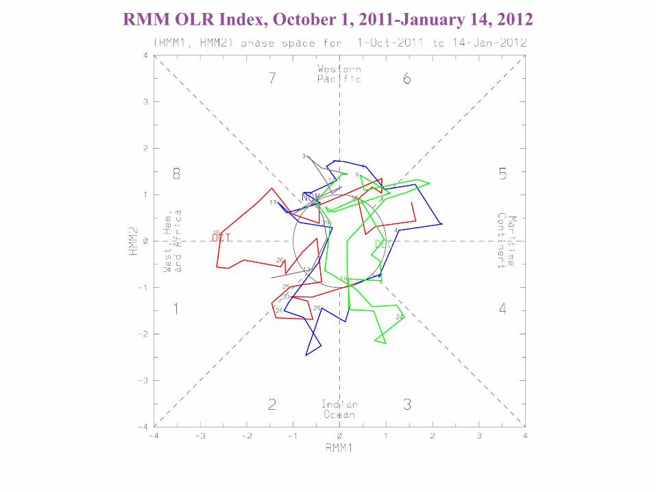
RMM OLR Index, October 1, 2011-January 14, 2012

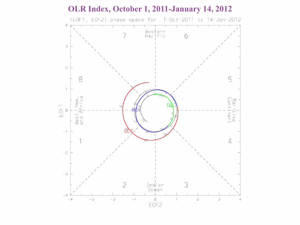
OLR Index, October 1, 2011-January 14, 2012

A disturbing result…but all is not lost!

Next we project the OLR PCs onto LESS FILTERED (20-96 day, all

wavenumbers westward and eastward) data:

OLR 20-96 Day Index, October 1, 2011-January 14, 2012

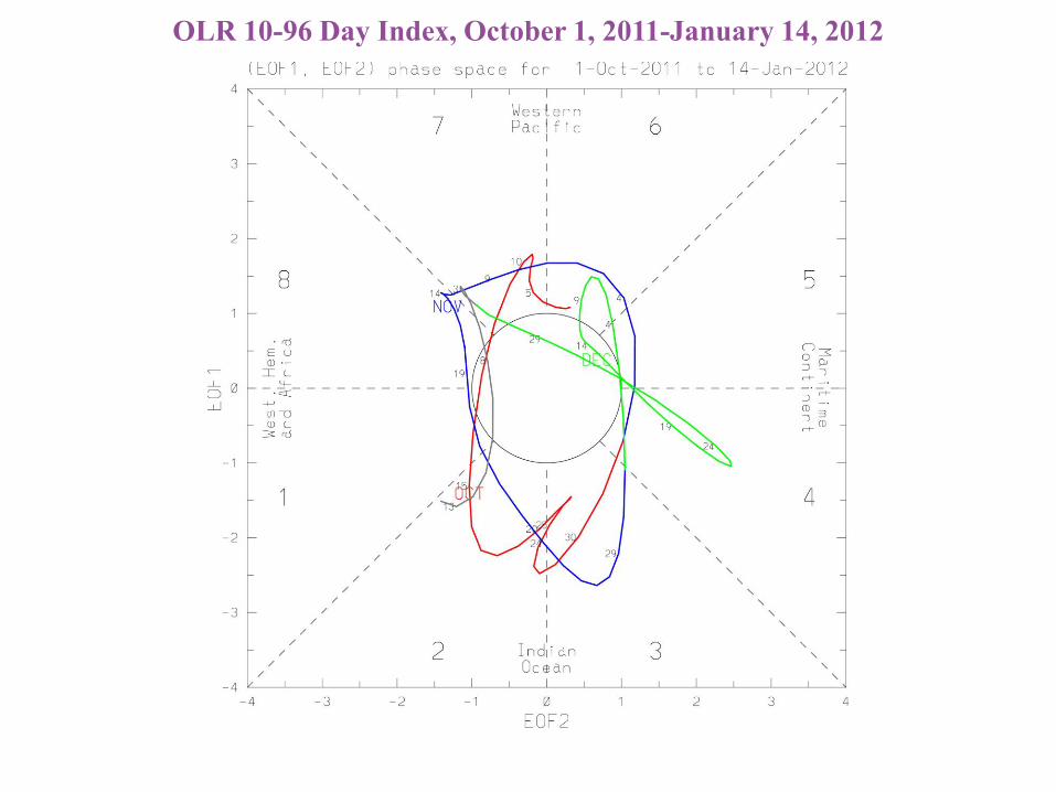
OLR 10-96 Day Index, October 1, 2011-January 14, 2012

OLR 2-96 Day Wavenumber 5 Index, October 1, 2011-January 14, 2012

OLR PC RMM RMM-OLR RMM-CIRC

.71 .69 .72

.69 .90

.67

Peak Correlations at Lag between OLR PCs and RMM PCs

OLR

PC

RMM

RMM-

OLR

RMM-

CIRC

Data Reconstruction

OLR data can be projected onto the PC indices:

OLR=PC1*EOF1 + PC2*EOF2

But…PCs don’t have to be derived from the original data…

Reconstructed OLR anomalies, 5ºS-5ºN, October 2011-January 2012

Reconstructed 20-96 Day OLR anomalies, 5ºS-5ºN, October 2011-January 2012

Advantages/Disadvantages of RMM Indices • Advantages:

• One set of patterns…seasonal cycle is still taken into account

• ENSO is accounted for

• Minimal filtering necessary

• Convenience! Easy to calculate retrospectively and in real time

• Straightforward for model calculations

• Disadvantages:

• Index is dominated by circulation at times

• Can be contaminated by higher frequency events (Kelvin waves)

• Antisymmetric signals across the equator lower the amplitude

• Noisy, although this could be mitigated by appropriate filtering

Advantages/Disadvantages of OLR EOF Index • Advantages:

• Much more related to convection itself, no circulation input

• Filters out Kelvin waves and other higher frequency events

• Tracks convection through the seasonal cycle

• Less noisy (depending upon the choice of filtering)

• Can be adapted for other modes

• Disadvantages:

• Less convenient to calculate, especially for real time

• ENSO can contaminate the results

• Model results would depend upon basic state biases

• Results are dependent on choice of filtering…less objective

Data Sources

Outgoing Longwave Radiation (OLR)

2 times daily, 2.5° resolution June 1974-May 2012

Cloud Archive User Services (CLAUS) Brightness Temperature

8 times daily, 1/3° resolution July 1983-September 2006

NCEP-NCAR Reanalysis products

4 times daily, up to 27 pressure levels, 2.5° resolution

January 1948-present

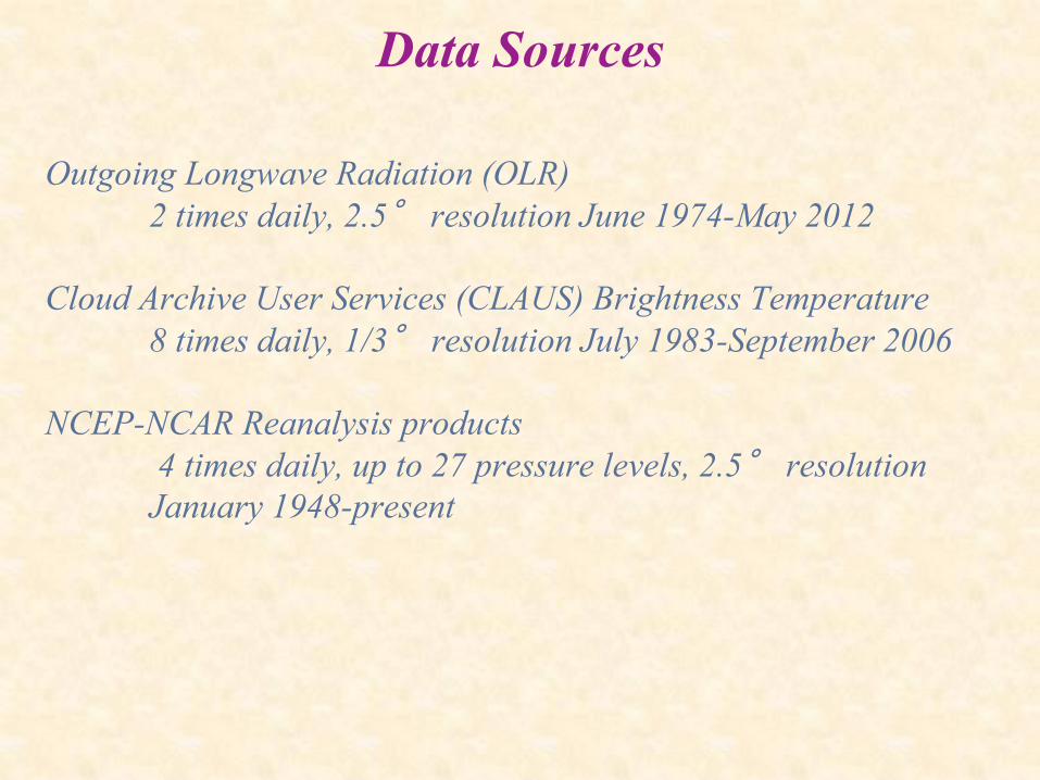
Data Sources

Outgoing Longwave Radiation (OLR)

2 times daily, 2.5° resolution June 1974-May 2012

Cloud Archive User Services (CLAUS) Brightness Temperature

8 times daily, 1/3° resolution July 1983-September 2006

NCEP-NCAR Reanalysis products

4 times daily, up to 27 pressure levels, 2.5° resolution

January 1948-present

For the purposes of this talk daily-averaged data are used…




for December-February (Regression Method)

OLR EOF

RMM

OLR anomalies, 5ºS-5ºN, October 2011-January 2012

a comparison of mjo indices for the dynamo field campaign · a comparison of mjo indices for the...

Documents