a comparison between 7- and 12-parameter shell finite
TRANSCRIPT
A COMPARISON BETWEEN 7- AND 12-PARAMETER SHELL FINITE
ELEMENTS FOR LARGE DEFORMATION ANALYSIS
A Dissertation
by
MIGUEL ERNESTO GUTIERREZ RIVERA
Submitted to the Office of Graduate and Professional Studies ofTexas A&M University
in partial fulfillment of the requirements for the degree of
DOCTOR OF PHILOSOPHY
Chair of Committee, Junuthula N. ReddyCommittee Members, Harry Hogan
Arun SrinivasaTheofanis Strouboulis
Head of Department, Andreas Polycarpou
December 2016
Major Subject: Mechanical Engineering
Copyright 2016 Miguel Ernesto Gutierrez Rivera

ABSTRACT
In this study two continuum shell finite elements are developed. The first one
is based on the first-order shear deformation theory with seven independent param-
eters and the second one is based on the third-order thickness deformation theory
with twelve independent parameters. Continuum shell finite elements are developed
and utilized in the numerical simulations of isotropic, laminated composite, and
functionally graded structures undergoing large deformations. High-order spectral
interpolation of the field variables is used to avoid all forms of numerical locking,
allowing the development of robust shell elements in a purely displacement based
setting.
This thesis includes static and transient analysis of various structures using afore-
mentioned two shell elements. This is the first time that the seven-parameter formu-
lation is used to compute a full transient response of shell structures. Deflections and
maximum stresses are computed and compared between the two formulations and,
in some cases, also with the results obtained using commercial codes ANSYS and
ABAQUS. Furthermore, the influence of the variation of the temperature through
the thickness for functionally graded shells is studied. In all the simulations, static
condensation of degrees of freedom associated with the internal nodes of the element
is implemented, which allows us to reduce the computational time and make use
of parallel computation when this feature is available. This makes the higher-order
elements used computationally competitive with standard finite elements.
ii

To my parents, my sister, my brothers, and my beloved girlfriend Erika
iii

ACKNOWLEDGEMENTS
I wish to express my gratitude to my advisor Dr. J. N. Reddy for his support
during my studies at Texas A&M University. Professor Reddy is an exceptional
person and an amazing researcher. It has been my genuine pleasure to work under
his supervision, to attend his courses, and to discuss my research with him.
I would like to thank to my committee members: Dr. Harry Hogan, Dr. Arun
Srinivasa and Dr. Theofanis Strouboulis. Professor Hogan kindly accepted to be part
of my dissertation committee. It was Professor Srinivasa who changed the way I see
the field of applied mechanics. I had the pleasure of taking my first graduate course
on the finite element method at Texas A&M University with Professor Strouboulis.
My sincere appreciation to Dr. Elias Ledesma and Dr. Abel Hernandez from
University of Guanajuato, for helping me contact Professor Reddy and their recom-
mendation to pursue my Ph.D. at Texas A&M University. Also, my sincere gratitude
to Dr. Marco Amabili, for accepting me as a Graduate Research Trainee at McGill
University. The principal subject of this dissertation was developed during that time.
I am grateful for the financial support given during my first semester by Professor
Reddy, who offered me a research assistantship, and for the rest of my studies by
the Mexican government through the “Consejo Nacional de Ciencia y Tecnologia”
(CONACYT) and the “Secretaria de Educacion Publica” (SEP).
The numerical simulations presented in Chapters 4 and 5 were made using the
Advanced Computational Mechanics Laboratory (ACML) cluster and the High Per-
formance Research Computing at Texas A&M University; their support is gratefully
acknowledged. I also want to recognize the comments and help of Professor Reddy’s
students during my Ph.D., and to his former students Dr. Gregory Payette and Dr.
iv
Roman Arciniega. Special thanks to Mr. Jinseok Kim for his friendship, and to Mr.
Michael Powell for his help using the ACML cluster.
My sincere recognition to my family and the support that they gave me during
all my studies. Thanks to my friends for always showing me the importance of fun
in life. Special thanks to my dear friends Sophie and Igor, for helping me during
all my studies at Texas A&M. Finally, I want to thank my beloved girlfriend Erika,
the most important person during my studies, for her love, patience, sacrifice and
support; I am truly grateful.
v

CONTRIBUTORS AND FUNDING SOURCES
Contributors
This work was supervised by a dissertation committee consisting of Professors
J.N. Reddy (advisor), Harry Hogan and Arun Srinivasa of the Department of Me-
chanical Engineering, and Professor Theofanis Strouboulis of the Department of
Aerospace Engineering.
All work for the dissertation was completed independently by the student.
Funding Sources
Graduate study was supported in Spring 2013 by a research assistantship offered
by Professor J.N. Reddy. All the other semesters were supported by the Mexican
government through the “Consejo Nacional de Ciencia y Tecnologia” (CONACYT)
and the “Secretaria de Educacion Publica” (SEP).
vi

TABLE OF CONTENTS
Page
ABSTRACT . . . . . . . . . . . . . . . . . . . . . . . . . . . . . . . . . . . . ii
DEDICATION . . . . . . . . . . . . . . . . . . . . . . . . . . . . . . . . . . . iii
ACKNOWLEDGEMENTS . . . . . . . . . . . . . . . . . . . . . . . . . . . . iv
CONTRIBUTORS AND FUNDING SOURCES . . . . . . . . . . . . . . . . . vi
TABLE OF CONTENTS . . . . . . . . . . . . . . . . . . . . . . . . . . . . . vii
LIST OF FIGURES . . . . . . . . . . . . . . . . . . . . . . . . . . . . . . . . x
LIST OF TABLES . . . . . . . . . . . . . . . . . . . . . . . . . . . . . . . . . xx
1. INTRODUCTION . . . . . . . . . . . . . . . . . . . . . . . . . . . . . . . 1
1.1 Background . . . . . . . . . . . . . . . . . . . . . . . . . . . . . . . . 11.2 Motivation for the present study . . . . . . . . . . . . . . . . . . . . . 31.3 Scope of the research . . . . . . . . . . . . . . . . . . . . . . . . . . . 5
2. LITERATURE REVIEW . . . . . . . . . . . . . . . . . . . . . . . . . . . 7
2.1 Equivalent single layer models . . . . . . . . . . . . . . . . . . . . . . 72.1.1 Classical shell model . . . . . . . . . . . . . . . . . . . . . . . 82.1.2 First-order Shear Deformation Theory . . . . . . . . . . . . . 82.1.3 Higher-order Shear Deformation Theories . . . . . . . . . . . . 9
2.2 Non-linear Higher-order Shear Deformation Theories . . . . . . . . . 112.3 High-Order Spectral/hp Finite Element Method . . . . . . . . . . . . 13
2.3.1 Introduction . . . . . . . . . . . . . . . . . . . . . . . . . . . . 132.3.2 Implementation . . . . . . . . . . . . . . . . . . . . . . . . . . 152.3.3 Static node condensation . . . . . . . . . . . . . . . . . . . . . 23
3. EQUATIONS OF MOTION . . . . . . . . . . . . . . . . . . . . . . . . . . 26
3.1 Parametrization of the shell . . . . . . . . . . . . . . . . . . . . . . . 273.2 Displacement fields . . . . . . . . . . . . . . . . . . . . . . . . . . . . 31
3.2.1 Seven-parameter formulation . . . . . . . . . . . . . . . . . . . 323.2.2 Twelve-parameter formulation . . . . . . . . . . . . . . . . . . 33
vii
3.3 Mechanical strains . . . . . . . . . . . . . . . . . . . . . . . . . . . . 343.4 Thermal strains . . . . . . . . . . . . . . . . . . . . . . . . . . . . . . 393.5 Stresses and constitutive equations . . . . . . . . . . . . . . . . . . . 41
3.5.1 Homogeneous isotropic shells . . . . . . . . . . . . . . . . . . 423.5.2 Functionally graded shells . . . . . . . . . . . . . . . . . . . . 433.5.3 Laminated composite shells . . . . . . . . . . . . . . . . . . . 45
3.6 Equations of motion . . . . . . . . . . . . . . . . . . . . . . . . . . . 48
4. STATIC ANALYSIS . . . . . . . . . . . . . . . . . . . . . . . . . . . . . . 52
4.1 Finite element model . . . . . . . . . . . . . . . . . . . . . . . . . . . 534.1.1 Newton’s method . . . . . . . . . . . . . . . . . . . . . . . . . 544.1.2 Arc-length method . . . . . . . . . . . . . . . . . . . . . . . . 57
4.2 Numerical examples . . . . . . . . . . . . . . . . . . . . . . . . . . . . 604.2.1 Isotropic square plate under uniformly distributed load . . . . 624.2.2 A simply supported isotropic cylindrical shell subjected to uni-
formly distributed radial forces . . . . . . . . . . . . . . . . . 684.2.3 Laminated composite plates under uniform pressure . . . . . . 724.2.4 Post-buckling response of laminated composite plate . . . . . 754.2.5 Static analysis of a functionally grade plate . . . . . . . . . . . 76
4.2.5.1 FGM plate under mechanical load . . . . . . . . . . 784.2.5.2 FGM plate under mechanical and thermal loads . . . 80
4.2.6 A cantilevered isotropic plate strip under an end shear force . 844.2.7 Roll-up of a clamped plate strip . . . . . . . . . . . . . . . . . 88
4.2.7.1 Isotropic . . . . . . . . . . . . . . . . . . . . . . . . . 914.2.7.2 Functionally graded . . . . . . . . . . . . . . . . . . 95
4.2.8 Torsion of a clamped plate strip . . . . . . . . . . . . . . . . . 964.2.9 Post-buckling of a plate strip . . . . . . . . . . . . . . . . . . 101
4.2.9.1 Isotropic . . . . . . . . . . . . . . . . . . . . . . . . . 1024.2.9.2 Laminated composite . . . . . . . . . . . . . . . . . . 1054.2.9.3 Functionally graded . . . . . . . . . . . . . . . . . . 107
4.2.10 A slit annular plate under an end shear force . . . . . . . . . . 1104.2.10.1 Isotropic . . . . . . . . . . . . . . . . . . . . . . . . . 1114.2.10.2 Laminated composite . . . . . . . . . . . . . . . . . . 1134.2.10.3 Functionally graded . . . . . . . . . . . . . . . . . . 115
4.2.11 Cylindrical panel under point load . . . . . . . . . . . . . . . 1174.2.11.1 Isotropic . . . . . . . . . . . . . . . . . . . . . . . . . 1174.2.11.2 Laminated composite . . . . . . . . . . . . . . . . . . 1184.2.11.3 Functionally graded . . . . . . . . . . . . . . . . . . 123
4.2.12 Pull-out of an open-ended cylindrical shell . . . . . . . . . . . 1244.2.12.1 Isotropic . . . . . . . . . . . . . . . . . . . . . . . . . 1264.2.12.2 Functionally graded . . . . . . . . . . . . . . . . . . 129
4.2.13 A pinched half-cylindrical shell . . . . . . . . . . . . . . . . . 131
viii

4.2.13.1 Isotropic . . . . . . . . . . . . . . . . . . . . . . . . . 1334.2.13.2 Laminated composite . . . . . . . . . . . . . . . . . . 134
4.2.14 A pinched hemisphere with an 18 hole . . . . . . . . . . . . . 1374.2.15 A pinched composite hyperboloidal shell . . . . . . . . . . . . 141
5. TRANSIENT ANALYSIS . . . . . . . . . . . . . . . . . . . . . . . . . . . 146
5.1 Finite element model . . . . . . . . . . . . . . . . . . . . . . . . . . . 1465.2 Numerical examples . . . . . . . . . . . . . . . . . . . . . . . . . . . . 148
5.2.1 Transient response of an isotropic plate . . . . . . . . . . . . . 1495.2.2 Transient response of a laminated composite plate . . . . . . . 1515.2.3 Transient response of a functionally graded plate . . . . . . . 1535.2.4 Transient response of an isotropic cylindrical shell . . . . . . . 1565.2.5 Transient response of a laminated composite clamped cylindri-
cal shell under internal pressure . . . . . . . . . . . . . . . . . 1615.2.6 Transient response of a functionally graded spherical shell . . 163
6. CONCLUSIONS AND FUTURE RESEARCH . . . . . . . . . . . . . . . . 169
6.1 Summary and concluding remarks . . . . . . . . . . . . . . . . . . . . 1696.2 Future research . . . . . . . . . . . . . . . . . . . . . . . . . . . . . . 171
REFERENCES . . . . . . . . . . . . . . . . . . . . . . . . . . . . . . . . . . . 174
ix
LIST OF FIGURES
FIGURE Page
2.1 One-dimensional C0 Lagrange interpolation functions φi for p = 4and 8, using equal and unequal nodal spacing having the commoncentral node. . . . . . . . . . . . . . . . . . . . . . . . . . . . . . . 14
2.2 One-dimensional C0 Lagrange interpolation functions φj of p = 8,with (a) equal and (b) unequal node () space. . . . . . . . . . . . 19
2.3 High-order spectral/hp quadrilateral master elements Ωe. . . . . . 20
2.4 Two-dimensional C0 Lagrange interpolation functions ψ41 of p = 8,with (a) equal and (b) unequal node space. . . . . . . . . . . . . . 21
2.5 Mesh for an hyperboloidal shell using p = 8. . . . . . . . . . . . . . 25
3.1 Approximation of the three dimensional shell element in the refer-ence configuration. . . . . . . . . . . . . . . . . . . . . . . . . . . . 29
3.2 Basis vectors aα and gα as well as the unit normal n shown in atypical shell element in the reference configuration. . . . . . . . . . 30
3.3 Strain measures versus stretch ratio. . . . . . . . . . . . . . . . . . 36
3.4 Variation of f+ through the thickness for different values of n. . . . 44
4.1 Node () and reduced integration point (×) locations in the masterelement for: (a) a 25-node element, p = 4, and (b) an 81-nodeelement, p = 8. . . . . . . . . . . . . . . . . . . . . . . . . . . . . . 61
4.2 Node () and reduced integration point (×) locations in the masterelement for the elements S4R in ABAQUS, and SHELL181 in ANSYS. 62
4.3 Simply supported aluminum square plate under uniform distributedload. . . . . . . . . . . . . . . . . . . . . . . . . . . . . . . . . . . 63
4.4 Maximum deflection uz(L/2, L/2)/h for a thin aluminum squareplate (h = 0.001 m). . . . . . . . . . . . . . . . . . . . . . . . . . . 64
x
4.5 Maximum rotation ϕx(0, L/2) for a thin aluminum square plate(h = 0.001 m). . . . . . . . . . . . . . . . . . . . . . . . . . . . . . 65
4.6 Thickness deformation in a thin aluminum square plate (h = 0.001m) when P = 1428.6. . . . . . . . . . . . . . . . . . . . . . . . . . 65
4.7 Deformed configuration of an isotropic thin plate under uniformpressure, h = 0.001 m and q = 1.05× 10⁸ Pa. . . . . . . . . . . . . 66
4.8 Maximum deflection uz(L/2, L/2)/h for a thick aluminum squareplate (h = 0.01 m). . . . . . . . . . . . . . . . . . . . . . . . . . . 66
4.9 Maximum rotation ϕx(0, L/2) for a thick aluminum square plate(h = 0.01 m). . . . . . . . . . . . . . . . . . . . . . . . . . . . . . . 67
4.10 Thickness deformation in a thick aluminum square plate (h = 0.01m) when P = 50. . . . . . . . . . . . . . . . . . . . . . . . . . . . . 67
4.11 Variation of the normal displacement across the thickness in a thickaluminum square plate (h = 0.01 m) at x/L = y/L = 0.5, whenP = 50. . . . . . . . . . . . . . . . . . . . . . . . . . . . . . . . . . 68
4.12 Isotropic cylinder with simply supported edges subjected to internalpressure. . . . . . . . . . . . . . . . . . . . . . . . . . . . . . . . . 69
4.13 Normalized radial displacement uz/h versus axial coordinate x/L. . 70
4.14 Normalized axial displacement ux/h versus axial coordinate x/L. . 70
4.15 Normalized thickness deformation versus axial coordinate x/L. . . 71
4.16 Rotation ϕx versus normalized axial coordinate x/L. . . . . . . . . 71
4.17 Deformed configuration of an isotropic cylinder under internal pres-sure, q = 198× 109 Pa. . . . . . . . . . . . . . . . . . . . . . . . . 72
4.18 A simply supported plate under uniform distributed load of inten-sity q. . . . . . . . . . . . . . . . . . . . . . . . . . . . . . . . . . . 72
4.19 Uniform pressure versus center deflection uz for a simply supportedplate. . . . . . . . . . . . . . . . . . . . . . . . . . . . . . . . . . . 74
4.20 Uniform pressure versus center deflection uz for a clamped plate. . 74
xi

4.21 A one side fixed and three side simply supported laminated plateunder uniform load of intensity P . . . . . . . . . . . . . . . . . . . 75
4.22 Normalized end shortening deflections versus nondimensionalizedload. . . . . . . . . . . . . . . . . . . . . . . . . . . . . . . . . . . 77
4.23 Normalized out of plane deflection versus nondimensionalized load. 77
4.24 Deformed configuration of a laminated plate after buckling (con-tours for uz at Pb = 98 kN). . . . . . . . . . . . . . . . . . . . . . 78
4.25 Uniform transverse load vs. normalized central deflection. . . . . . 79
4.26 Dimensionless axial stress along the thickness, at the center of theplates under the dimensionless load Q = −400. . . . . . . . . . . . 80
4.27 Temperature field through the thickness of the FG plates. . . . . . 81
4.28 Uniform transverse load vs. normalized central deflection of FGplates under mechanical and thermal loads. . . . . . . . . . . . . . 81
4.29 Dimensionless axial stress along the thickness, at the center of theplates under the dimensionless load Q = −80 and thermal load. . . 82
4.30 Cantilever plate strip under an end shear force. . . . . . . . . . . . 85
4.31 End shear force q vs. tip-deflection ux, for an isotropic cantileveredplate strip (ν = 0.0). . . . . . . . . . . . . . . . . . . . . . . . . . . 85
4.32 End shear force q vs. tip-deflection uz, for an isotropic cantileveredplate strip (ν = 0.0). . . . . . . . . . . . . . . . . . . . . . . . . . . 86
4.33 Deformed configurations of an isotropic cantilever plate strip sub-jected to an end shear force (load values q = 0.0, 1.0, ..., 5.0). . . . . 86
4.34 Plots of the maximum stress, σxx, at point A: (0.3125, 0.375, −h/2)versus load q, for an isotropic cantilevered plate strip (ν = 0.0). . . 87
4.35 Plots of the maximum stress, σzz, at point B: (4.0625, 0.375, −h/2)versus load q, for an isotropic cantilevered plate strip (ν = 0.0). . . 88
4.36 End shear force q vs. tip-deflection ux, for an isotropic cantileveredplate strip (ν = 0.3). . . . . . . . . . . . . . . . . . . . . . . . . . . 89
xii
4.37 End shear force vs. tip-deflection uz, for an isotropic cantileveredplate strip (ν = 0.3). . . . . . . . . . . . . . . . . . . . . . . . . . . 89
4.38 Plots of the stress, σxx, at point C: (4.0625, 0.875, −h/2) versusload q, for an isotropic cantilevered plate strip (ν = 0.3). . . . . . . 90
4.39 Plots of the maximum stress, σzz, at point C: (4.0625, 0.875, −h/2)versus load q, for an isotropic cantilevered plate strip (ν = 0.3). . . 90
4.40 Cantilever plate strip under an end moment. . . . . . . . . . . . . 91
4.41 End moment vs. tip-deflection ux, for an isotropic cantileveredplate strip. . . . . . . . . . . . . . . . . . . . . . . . . . . . . . . . 92
4.42 End moment vs. tip-deflection uz, for an isotropic cantileveredplate strip. . . . . . . . . . . . . . . . . . . . . . . . . . . . . . . . 93
4.43 Undeformed and deformed configurations of an isotropic cantileverplate strip subjected to an end moment (load values M/Mmax =0.1, 0.2, ..., 1). . . . . . . . . . . . . . . . . . . . . . . . . . . . . . . 93
4.44 End moment vs. stress σxx(11.8125, 0.875,−h/2), for an isotropiccantilevered plate strip. . . . . . . . . . . . . . . . . . . . . . . . . 94
4.45 End moment vs. stress σzz (3.1875, 0.625, -h/2), for an isotropiccantilevered plate strip. . . . . . . . . . . . . . . . . . . . . . . . . 94
4.46 End moment vs. tip-deflection ux, for various functionally gradedplates. . . . . . . . . . . . . . . . . . . . . . . . . . . . . . . . . . . 96
4.47 End moment vs. tip-deflection uz, for various functionally gradedplates. . . . . . . . . . . . . . . . . . . . . . . . . . . . . . . . . . . 96
4.48 Plots of the maximum stress, σxx, at point A: (25L/64, 7b/8, −h/2)versus end moment, for various functionally graded plates. . . . . . 97
4.49 Plots of the maximum stress, σzz, at point B: (49L/64, 7b/8, −h/2)versus end moment, for various functionally graded plates. . . . . . 97
4.50 Cantilever plate strip under an end torsional moment. . . . . . . . 98
4.51 End torsion moment versus tip-deflection uz at point A. . . . . . . 99
4.52 End torsion moment versus tip-deflection uz at point B. . . . . . . 100
xiii
4.53 Deformed configuration at the maximum load achieved for the: (a)7- (T = 1000) and (b) 12-parameter (T = 820) formulations. . . . . 100
4.54 End torsion moment versus stress σxx. . . . . . . . . . . . . . . . . 101
4.55 A cantilevered strip plate subjected at its free end to a compressiveaxial force. . . . . . . . . . . . . . . . . . . . . . . . . . . . . . . . 102
4.56 Compressive load P vs. tip-deflection, for an isotropic cantileveredplate strip. . . . . . . . . . . . . . . . . . . . . . . . . . . . . . . . 103
4.57 Undeformed and deformed configurations of an isotropic cantileverstrip plate subjected to an axial load (P = 1.125, 1.250, 2, 3, 4, 5,6 and 7 kN). . . . . . . . . . . . . . . . . . . . . . . . . . . . . . . 104
4.58 Compressive load P vs. stress σxx(L/64, 5b/16, −h/2), for anisotropic cantilevered plate strip. . . . . . . . . . . . . . . . . . . . 104
4.59 Undeformed and deformed configurations of an isotropic cantileverstrip plate subjected to an axial load: (a) P = 11.67, and (b)P = 37.33 kN. . . . . . . . . . . . . . . . . . . . . . . . . . . . . . 105
4.60 Compressive load P vs. tip-deflection ux, for various laminatedcomposite plates. . . . . . . . . . . . . . . . . . . . . . . . . . . . . 106
4.61 Compressive load P vs. tip-deflection uz, for various laminatedcomposite plates. . . . . . . . . . . . . . . . . . . . . . . . . . . . . 107
4.62 Deformed configuration of a laminated composite (30/-60/-60/30)cantilever strip plate subjected to an axial load (P = 1000 N). . . . 107
4.63 Compressive load P vs. stress σxx(L/64, 5b/16, −h/2), for variouslaminated composite plates. . . . . . . . . . . . . . . . . . . . . . . 108
4.64 Compressive load P vs. tip-deflection ux, for various functionallygraded plates. . . . . . . . . . . . . . . . . . . . . . . . . . . . . . 109
4.65 Compressive load P vs. tip-deflection uz, for various functionallygraded plates. . . . . . . . . . . . . . . . . . . . . . . . . . . . . . 109
4.66 Compressive load P vs. bending stress σxx(L/64, 5b/16, −h/2), forvarious functionally graded plates. . . . . . . . . . . . . . . . . . . 110
4.67 Annular plate strip under transverse end shear force. . . . . . . . . 111
xiv
4.68 Pulling force versus vertical displacement, uz ( ANSYS and ABAQUS), for an isotropic annular plate. . . . . . . . . . . . . . . 112
4.69 Undeformed and deformed configurations of an isotropic circularplate strip under transverse shear force (F = 2.5, 5.0, ..., 20.0). . . . 112
4.70 End shear force F vs. stress σxx, for an isotropic annular plate. . . 113
4.71 Pulling force versus vertical displacement, uz, at point B, for variouslaminated composite annular plates. . . . . . . . . . . . . . . . . . 114
4.72 Pulling force versus stress σxx, for various laminated composite an-nular plates. . . . . . . . . . . . . . . . . . . . . . . . . . . . . . . 115
4.73 Pulling force versus vertical displacement, uz, at point B, for variousfunctionally graded annular plates. . . . . . . . . . . . . . . . . . . 116
4.74 Plots of the maximum stress, σxx, at point C: (7.25, 39π/32, +h/2)versus load F , for various functionally graded annular plates. . . . 116
4.75 A shallow cylindrical panel subjected to a point load at its center. 118
4.76 Vertical deflection of isotropic shallow cylindrical panels under pointloading. . . . . . . . . . . . . . . . . . . . . . . . . . . . . . . . . . 119
4.77 Deformed configuration of an isotropic cylindrical panel, h = 6.35mm and P = 4000 N. . . . . . . . . . . . . . . . . . . . . . . . . . 119
4.78 Point load P vs. stress σyy(R − h/2, π/160, 15a/32) of isotropicshallow cylindrical panels under point loading. . . . . . . . . . . . 120
4.79 Vertical deflection of laminated composite shallow cylindrical pan-els under point loading, h = 12.7 mm. . . . . . . . . . . . . . . . . 121
4.80 Vertical deflection of laminated composite shallow cylindrical pan-els under point loading, h = 6.35 mm. . . . . . . . . . . . . . . . . 121
4.81 Point load P vs. stress σyy(R − h/2, π/160, 15a/32) of laminatedcomposite shallow cylindrical panels under point loading, h = 12.7mm. . . . . . . . . . . . . . . . . . . . . . . . . . . . . . . . . . . . 122
4.82 Point load P vs. stress σyy(R − h/2, π/160, 15a/32) of laminatedcomposite shallow cylindrical panels under point loading, h = 6.35mm. . . . . . . . . . . . . . . . . . . . . . . . . . . . . . . . . . . . 122
xv
4.83 Vertical deflection of functionally graded shallow cylindrical panelsunder point loading, h = 12.7 mm. . . . . . . . . . . . . . . . . . . 123
4.84 Vertical deflection of functionally graded shallow cylindrical panelsunder point loading, h = 6.35 mm. . . . . . . . . . . . . . . . . . . 124
4.85 Point load P versus stress σyy(R − h/2, π/160, 15a/32) of func-tionally graded shallow cylindrical panels under point loading, h =12.7 mm. . . . . . . . . . . . . . . . . . . . . . . . . . . . . . . . . 125
4.86 Point load P versus stress σyy(R − h/2, π/160, 15a/32) of func-tionally graded shallow cylindrical panels under point loading, h =6.35 mm. . . . . . . . . . . . . . . . . . . . . . . . . . . . . . . . . 125
4.87 Pull-out of a cylinder with free edges. . . . . . . . . . . . . . . . . 126
4.88 Point load P vs. radial deflection at different points of an isotropiccylinder with free edges (results using ANSYS , and ABAQUS ). 127
4.89 Point load P vs. stress σxx of an isotropic cylinder with free edges. 127
4.90 Point load P vs. stress σzz of an isotropic cylinder with free edges. 128
4.91 Pulling force versus radial displacements at point A of a functionallygraded cylinder with free edges. . . . . . . . . . . . . . . . . . . . . 130
4.92 Pulling force versus radial displacements at point B of a functionallygraded cylinder with free edges. . . . . . . . . . . . . . . . . . . . . 130
4.93 Pulling force versus radial displacements at point C of a functionallygraded cylinder with free edges. . . . . . . . . . . . . . . . . . . . . 131
4.94 Deformed configuration of the functionally graded cylindrical shellunder pulling forces. Load P = 5× 10⁶ and n = 1.0. . . . . . . . . 131
4.95 Plots of the maximum stress, σxx(R + h/2, π/64, 29L/64) versusload P of a functionally graded cylinder with free edges. . . . . . . 132
4.96 Plots of the maximum stress, σzz(R + h/2, π/64, 25L/64) versusload P of a functionally graded cylinder with free edges. . . . . . . 132
4.97 Clamped semi-cylindrical shell under point load. . . . . . . . . . . 133
4.98 Vertical deflection at point A of an isotropic half-cylindrical shellsunder point loading. . . . . . . . . . . . . . . . . . . . . . . . . . . 134
xvi

4.99 Maximum stress σxx (R + h/2, π/64, 61L/64) vs. point load P foran isotropic half-cylindrical shell. . . . . . . . . . . . . . . . . . . . 135
4.100 Maximum stress σzz (R + h/2, π/64, 63L/64) vs. point load P foran isotropic half-cylindrical shell. . . . . . . . . . . . . . . . . . . . 135
4.101 Vertical deflection at point A for a (90/0/90) and (0/90/0)laminated composite half-cylindrical shells under point loading, rep-resented by black and blue lines, respectively. . . . . . . . . . . . . 136
4.102 Deformed configuration of a laminated composited pinched halfcylindrical shell (90/0/90) for P = 2× 10⁴ N. . . . . . . . . . . 137
4.103 Stress σzz (R+h/2, π/64, 63L/64) vs. point load P for a laminatedcomposite (90/0/90) half-cylindrical shell. . . . . . . . . . . . . 138
4.104 Maximum stress σzz (R + h/2, π/64, 63L/64) vs. point load P fora laminated composite (0/90/0) half-cylindrical shell. . . . . . . 138
4.105 Pinched hemispherical shell with 18 hole. . . . . . . . . . . . . . . 139
4.106 Radial deflections at points B and C of the pinched hemisphere (ABAQUS, and ANSYS). . . . . . . . . . . . . . . . . . . . . . . 140
4.107 Deformed configuration of a pinched hemispherical shell for P =900 lb. . . . . . . . . . . . . . . . . . . . . . . . . . . . . . . . . . 140
4.108 Pulling force P versus stress σyy of the pinched hemisphere. . . . . 141
4.109 Hyperboloidal shell. . . . . . . . . . . . . . . . . . . . . . . . . . . 142
4.110 Pulling force versus radial displacements at different points for apinched (0/90/0) stacking sequence laminated composite hyper-boloidal shell. . . . . . . . . . . . . . . . . . . . . . . . . . . . . . . 143
4.111 Pulling force versus radial displacements at different points for apinched (90/0/90) stacking sequence laminated composite hy-perboloidal shell. . . . . . . . . . . . . . . . . . . . . . . . . . . . . 143
4.112 Deformed configuration of a pinched laminated composite hyper-boloidal shell (90/0/90) for P = 480. . . . . . . . . . . . . . . . 144
4.113 Pulling force versus the stress σyy for the (0/90/0) stacking se-quence. . . . . . . . . . . . . . . . . . . . . . . . . . . . . . . . . . 145
xvii

4.114 Pulling force versus the stress σzz for the (90/0/90) stackingsequence. . . . . . . . . . . . . . . . . . . . . . . . . . . . . . . . . 145
5.1 Center deflection w vs. time t for a simply supported square plateunder uniform load. . . . . . . . . . . . . . . . . . . . . . . . . . . 151
5.2 Deformed configuration of an isotropic simply supported plate un-der uniform load, at t = 180µs. . . . . . . . . . . . . . . . . . . . . 151
5.3 Time t vs. bending stress σxx(L/32, L/32, −h/2). . . . . . . . . . 152
5.4 Center deflection w vs. time t for a simply supported square plateunder uniform load. . . . . . . . . . . . . . . . . . . . . . . . . . . 153
5.5 Stress σxx vs. time t for a simply supported square plate underuniform load. . . . . . . . . . . . . . . . . . . . . . . . . . . . . . . 154
5.6 Temporal evolution of center deflection of a simply supported func-tionally graded plate under a suddenly applied uniform load q. . . 156
5.7 Temporal evolution of center deflection of a simply supported func-tionally graded plate under a suddenly applied uniform load q andtemperature field. . . . . . . . . . . . . . . . . . . . . . . . . . . . 156
5.8 Temporal evolution of non-dimensional stress σxx of a simply sup-ported functionally graded plate under a suddenly applied uniformload q. . . . . . . . . . . . . . . . . . . . . . . . . . . . . . . . . . 157
5.9 Temporal evolution of non-dimensional stress σxx of a simply sup-ported functionally graded plate under a suddenly applied uniformload q and temperature field. . . . . . . . . . . . . . . . . . . . . . 157
5.10 A shallow cylindrical panel subjected to a point load at its center. 159
5.11 Center deflection vs. time t for a simply supported cylindrical shellunder a point load P . . . . . . . . . . . . . . . . . . . . . . . . . . 159
5.12 Deformed configurations for different time for an isotropic cylindri-cal shell under a point load. . . . . . . . . . . . . . . . . . . . . . . 160
5.13 Stress σxx vs. time t for a simply supported cylindrical shell undera point load P . . . . . . . . . . . . . . . . . . . . . . . . . . . . . . 161
5.14 Laminated composite cylinder with fixed edges subjected to inter-nal pressure. . . . . . . . . . . . . . . . . . . . . . . . . . . . . . . 162
xviii
5.15 Center deflection vs. time t for a clamped composite cylindricalshell (0/90) under a distributed load q. . . . . . . . . . . . . . . 163
5.16 Deformed configuration for a laminated cylindrical shell under auniform distributed load, at t = 0.027 s. . . . . . . . . . . . . . . . 164
5.17 Stress σyy vs. time t for a clamped composite cylindrical shell(0/90) under a uniformly distributed load q. . . . . . . . . . . . . 164
5.18 Clamped spherical shell under a uniform distributed load q. . . . . 165
5.19 Temporal evolution of center deflection of a clamped functionallygraded shell under a suddenly applied uniform load q. . . . . . . . 166
5.20 Deformed configuration for a functionally graded spherical shell(n = 2) under a uniformly distributed load, at t = 246 µs. . . . . . 167
5.21 Temporal evolution of center deflection of a clamped functionallygraded shell under a suddenly applied uniform load q and temper-ature field. . . . . . . . . . . . . . . . . . . . . . . . . . . . . . . . 167
5.22 Temporal evolution of the non-dimensional stress σxx of a clampedfunctionally graded shell under a suddenly applied uniform load q. 168
5.23 Temporal evolution of the non-dimensional stress σxx of a clampedfunctionally graded shell under a suddenly applied uniform load qand temperature field. . . . . . . . . . . . . . . . . . . . . . . . . . 168
xix

LIST OF TABLES
TABLE Page
2.1 Comparison between the formulations presented and commercialcodes. . . . . . . . . . . . . . . . . . . . . . . . . . . . . . . . . . . 25
4.1 Material properties of aluminum and alumina. . . . . . . . . . . . 79
4.2 Comparison between the results obtained using the presented mod-els, the classical plate theory, and solid elements in ANSYS andABAQUS. . . . . . . . . . . . . . . . . . . . . . . . . . . . . . . . 83
4.3 Number of nodes, total degrees of freedom (DOF), and compu-tational time used (for the presented models, and solid elementsin ANSYS and ABAQUS) to solve a ceramic plate under thermo-mechanical loads. . . . . . . . . . . . . . . . . . . . . . . . . . . . 84
4.4 Number of nodes, total degrees of freedom (DOF), and compu-tational time used (for the presented models, and solid elementsin ANSYS and ABAQUS) to solve an open-ended cylindrical shellunder a point load. . . . . . . . . . . . . . . . . . . . . . . . . . . . 129
xx

1. INTRODUCTION
1.1 Background
Shell structures are the most efficient structures used in engineering, for instance,
they are found in roofs, bridges, bodies of cars and airplanes, rockets, and ship hulls,
just to name a few. In these cases, a thin structure covers a wide area and holds large
external loads, making it possible to create a light structure and to use the minimum
amount of material required [1, 2]. Due to their importance, shells have been widely
analyzed and numerous shell theories and finite element models are proposed in the
literature.
The differential equations of three-dimensional elasticity can be used to model
the shell behavior. However, solutions are very complex and higher computational
resources are needed, that is why solutions are restricted to simple cases or to validate
models [3]. To overcome these problems, shell theories have emerged as an efficient
way to model shell structures as a two-dimensional problem, but these theories have
some limitations, depending of the level of approximation.
The simplest theory is the classical, also known as Kirchhoff–Love, which neglects
shear deformation, and transverse shear as well as transverse normal strains, being
well suited for thin shells. To overcome this limitation shear deformation theories
have been developed, which can be divided into first- and higher-order shear defor-
mation theories [4, 5]. In the first kind, the use of a shear correction factor is enforced
since uniform shear strains are assumed through the thickness, but it is not necessary
in the latter theory by assuming a realistic shear stress distribution through the shell
thickness.
Even though the use of higher-order shear deformation theories started in the
1
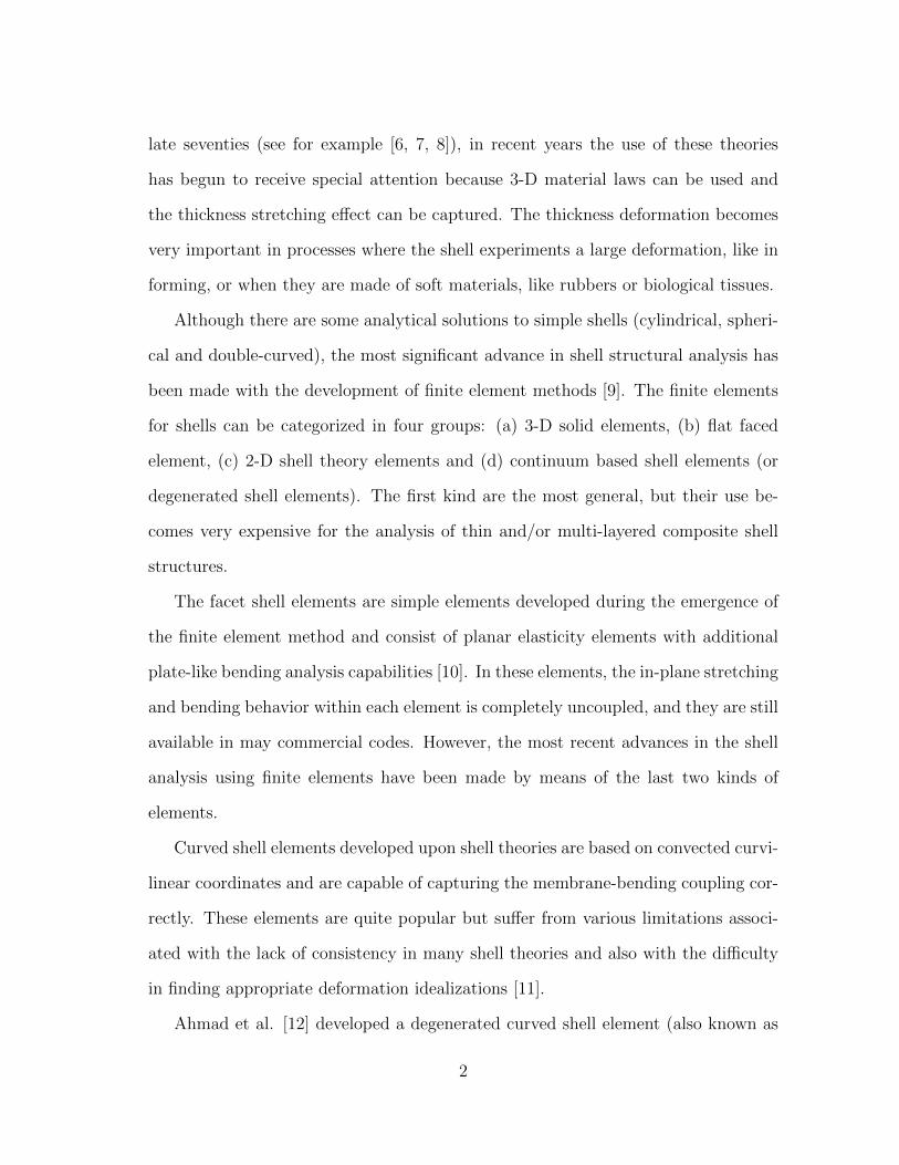
late seventies (see for example [6, 7, 8]), in recent years the use of these theories
has begun to receive special attention because 3-D material laws can be used and
the thickness stretching effect can be captured. The thickness deformation becomes
very important in processes where the shell experiments a large deformation, like in
forming, or when they are made of soft materials, like rubbers or biological tissues.
Although there are some analytical solutions to simple shells (cylindrical, spheri-
cal and double-curved), the most significant advance in shell structural analysis has
been made with the development of finite element methods [9]. The finite elements
for shells can be categorized in four groups: (a) 3-D solid elements, (b) flat faced
element, (c) 2-D shell theory elements and (d) continuum based shell elements (or
degenerated shell elements). The first kind are the most general, but their use be-
comes very expensive for the analysis of thin and/or multi-layered composite shell
structures.
The facet shell elements are simple elements developed during the emergence of
the finite element method and consist of planar elasticity elements with additional
plate-like bending analysis capabilities [10]. In these elements, the in-plane stretching
and bending behavior within each element is completely uncoupled, and they are still
available in may commercial codes. However, the most recent advances in the shell
analysis using finite elements have been made by means of the last two kinds of
elements.
Curved shell elements developed upon shell theories are based on convected curvi-
linear coordinates and are capable of capturing the membrane-bending coupling cor-
rectly. These elements are quite popular but suffer from various limitations associ-
ated with the lack of consistency in many shell theories and also with the difficulty
in finding appropriate deformation idealizations [11].
Ahmad et al. [12] developed a degenerated curved shell element (also known as
2

continuum shell), by means of the discretization of the 3-D elasticity equations in
terms of mid-surface nodal variables. In this work, we use this approach and we show
that it is very efficient and simple to implement for the two formulations presented
here.
The finite element implementation of the last three shell groups, using low-order
shape functions and displacement based formulations, suffers from various forms
of locking, like the transverse shear-, membrane- and volume-locking [13]. This
phenomenon arises due to inconsistencies in modeling the transverse shear energy and
membrane energy, or when the shell elements include thickness change, respectively.
Some forms to avoid it are the use of selective or reduced integration [14, 15], Hu-
Washizu type mixed variational principles [16, 17], and assumed strain [18, 19] or
enhanced strain [20] formulations.
Another way to avoid the locking is the use of high-order shape functions, in the
same displacement based formulations [21]. Relevant works are the tensor-based fi-
nite element shell with first-order shear deformation theory and seven parameters by
Arciniega and Reddy [22, 23], and a similar work by Payette and Reddy [24] where
continuous shell elements in conjunction with high order spectral/hp functions were
implemented. We adopt the latter approach using the same type of shape func-
tions, which presents several advantages, compared with Lagrangian interpolation
functions, as will be shown in Chapter 2.
1.2 Motivation for the present study
After a literature review of the previous works for the analysis of shells, we find
that most shell formulations are based on mixed formulations, and are implemented
using low-order finite elements. Only a few works have explored the advantages of
the higher-order interpolation functions on shells. This feature avoids the use of
3

selective or reduced integration or other numerical tricks, in a purely displacement
based formulation. Also, the spectral functions reduce the oscillation presented in
the traditional Lagrange interpolation functions near the end points.
In addition, the traditional elements cannot capture the thickness deformation,
since the assumption of plane stress is made. The use of higher-order shear defor-
mation theories can alleviate this constrain, and allow the use of 3-D constitutive
equations. In recent works Amabili [25, 26] presented a high-order shear deforma-
tion theory using third-order thickness stretching kinematics and retaining non-linear
terms in the in plane and transverse displacements. He showed that for highly loaded
shells with significant thickness stretching, or for shells made of soft materials that
present large strains, these assumptions are important to predict the non-linear dy-
namic response of shells, specially near the edges. In those works, the solutions were
obtained using numerical series for cylindrical shells.
Based on the benefits of higher-order spectral/hp basis functions, and the advan-
tages of higher-order shear deformation theories, we develop a computational model
to analyze the nonlinear static and transient response of shells, using a third-order
thickness stretching theory with twelve independent parameters, and also explore
the influence of temperature in the mechanical response of functionally graded shells.
Furthermore, we extend the work of Payette and Reddy [24] for the static analysis
of shells, based on the first-order shear deformation theory with seven independent
parameters, to compare with our results. In both instances, we use three dimen-
sional constitutive equations in conjunction with a continuum shell element model
and high-order spectral/hp basis functions that allow a highly accurate representa-
tion of arbitrary shell geometries and yield reliable numerical results that are locking
free.
In addition, most of the previous works on large deformation analysis only report
4
deformations. Even when these are quantities that can be measured directly, in the
process of design one of the most important aspects is the stress analysis. For this
reason, we also develop a subroutine to compute the Cauchy stresses and present the
results that can be used as reference in future investigations.
1.3 Scope of the research
This research began at Texas A&M in the Spring 2013 and is focused on the
development of finite element models for shell elements using high-order spectral/hp
approximation functions. The research encompasses the weak-form Galerkin finite
element models for elastic shells, using seven [27] and twelve [28] independent param-
eters for isotropic, laminated composite, and functionally graded materials. Static
and transient analyses are performed, and for functionally graded shells the influence
of the temperature through the thickness in the mechanical response is also included.
The dissertation is organized as follows. In Chapter 2 we present a review on the
development of shell and plate theories, making special emphasis on the high-order
shear deformation theories. We list the most significant contributions and remark
those that influence this work. We also give an overview of the high-order spectral
functions and their application to the shell elements. Furthermore, we give a brief
description about the static-node condensation; an important feature that allows to
reduce computational time.
In Chapter 3 we introduce the parameterization of the shell mid-surface, and we
present a brief description of the Taylor series expansion to describe the displace-
ment vector, and how it can be used to obtain the two formulations discussed here.
Then, we present the measures for mechanical strains, and we justify the selection
of the Green–Lagrange strain and its limitations. Also, the thermal strains for large
deformation are discussed and the assumptions made to linearize them. After that,
5
we discuss the constitutive equations for the three materials considered along this
dissertation, and the process to compute Cauchy stresses. Finally, we describe the
equations of motion for shells using 7- and 12-parameter formulations.
In Chapters 4 and 5 we present the weak form of the formulations presented in this
work, and describe the methods used to solve the problems for static and transient
analysis, respectively. Furthermore, we perform some comparisons with analytical
solutions, experimental data, commercial codes ANSYS and ABAQUS, as well as
some benchmark problems taken from the literature, where the structures undergo
large deformations. Displacements and Cauchy stresses are computed for these struc-
tures. Finally, in Chapter 6 we provide concluding remarks and recommendations
for future research.
6

2. LITERATURE REVIEW
In this chapter, we review the historical development of plate and shell analysis
by means of the equivalent single layer (ESL) theories. We present the assumptions
and general equations in each case. Note that there is extensive literature about
these theories and, for that reason, we only cite some classical papers and those
which constitute a background for the present work.
After that, we present a general overview of the high-order spectral/hp finite
element, and its implementation for shells. We also discuss some important aspects
found during the development of this investigation. Later, we present the notation
and general aspects used in the finite element discretization, and we recall some
definitions and properties of the spectral elements. Finally, we present the static
node condensation, an important feature that allows these elements to compete,
based on the computational time, with standard low-order elements.
2.1 Equivalent single layer models
The equivalent single layer models are derived from the three dimensional elas-
ticity theory by making assumptions on the kinematics of deformation or the stress
state through the thickness of the laminate [4]. The simplest ESL model is based on
the Love hypothesis [29], which ignores shear and normal deformations and is only
suitable for thin shells. The next ESL model is the first-order shear deformation
theory (FSDT) developed by Mindlin [30], which accounts for the shear deformation
effect by means of a linear variation of in-plane displacements through the thickness,
and therefore a shear correction factor is required. To avoid the use of this factor,
higher-order shear deformation theories (HSDT), the next ESL model in hierarchy,
were introduced, and can be developed by expanding the displacement components
7

in power series of the thickness coordinate. In the following subsections we give more
details about these models.
2.1.1 Classical shell model
Classical shell models are based on the kinematic assumption that any material
line that is orthogonal to the mid-surface in the undeformed configuration remains
straight and unstretched during the deformation [31]. This assumption is based on
the displacement field in the form
u(ξ1, ξ2, ξ3, t) =u0(ξ1, ξ2, t)− ξ3∂w0
∂ξ1(2.1)
v(ξ1, ξ2, ξ3, t) =v0(ξ1, ξ2, t)− ξ3∂w0
∂ξ2(2.2)
w(ξ1, ξ2, ξ3, t) =w0(ξ1, ξ2, t) (2.3)
where u0, v0 and w0 are the components of the mid-plane displacements in the ξ1,
ξ2 and ξ3 directions, respectively.
This is called the Kirchhoff–Love hypothesis and implies the vanishing of the shear
and normal strains, neglecting the shear and normal deformation. That is why, it
is only suitable for thin plates and shells, where the shear and normal deformation
effects are negligible [32]. Furthermore, the use of C1 continuous functions is required,
becoming computationally inefficient from the point of view of simple finite element
formulations [33].
2.1.2 First-order Shear Deformation Theory
If a linear variation of the displacement through the thickness is considered,
the shear deformation can be taken into account. This assumption is known as
the Reissner-Mindlin theory (see Reissner[34] and Mindlin [30]). However, these
8

theories have profound differences in assumptions and formulations, further details
can be found in the paper of Wang et al. [35]. For this reason, we refer to it as
the First-order Shear Deformation Theory (FSDT), which is originally based on the
displacement field
u(ξ1, ξ2, ξ3, t) =u0(ξ1, ξ2, t) + ξ3u1(ξ1, ξ2, t) (2.4)
v(ξ1, ξ2, ξ3, t) =v0(ξ1, ξ2, t) + ξ3v1(ξ1, ξ2, t) (2.5)
w(ξ1, ξ2, ξ3, t) =w0(ξ1, ξ2, t) (2.6)
where u0, v0 and w0 are the components of the mid-plane displacements, and u1 and
v1 denote rotations of a normal to the reference surface about the ξ2, and ξ1 axes,
respectively
u1 =∂u0
∂ξ3, v1 =
∂v0
∂ξ3. (2.7)
In the FSDT the transverse strain is constant through the thickness, behavior that
is opposite to the actual physics, and a shear correction factor is needed [36]. Since
the variables in this formulation are independent, its finite element formulation can
be made using only C0 continuity functions.
2.1.3 Higher-order Shear Deformation Theories
The two previous models also include the hypothesis of a plane stress state tangent
to the mid-surface of the shell [37]. These models can handle simple analysis in shells
satisfactorily. However, in processes where the deformations are large or there is a
considerable change in the thickness, like in metal forming, they cannot reproduce the
behavior, since the normal stress in the thickness direction is omitted [38]. Moreover,
these theories do not include cross-section warping which becomes significant in thick
9

plates and shells [39].
To overcome these problems, Higher-order Shear Deformation Theories (HSDT)
have been introduced [4, 5], that may be employed with unmodified fully three di-
mensional constitutive equations and the use of a shear correction factor is avoided.
These formulations also take into account the change in thickness and can be used
to model thin and thick shells. The displacement components through the thickness
are expanded by polynomials, as
u(ξ1, ξ2, ξ3, t) =u0(ξ1, ξ2, t) + ξ3u1(ξ1, ξ2, t) + (ξ3)2u2(ξ1, ξ2, t)
+ (ξ3)3u3(ξ1, ξ2, t) + . . . (2.8)
v(ξ1, ξ2, ξ3, t) =v0(ξ1, ξ2, t) + ξ3v1(ξ1, ξ2, t) + (ξ3)2v2(ξ1, ξ2, t)
+ (ξ3)3v3(ξ1, ξ2, t) + . . . (2.9)
w(ξ1, ξ2, ξ3, t) =w0(ξ1, ξ2, t) + ξ3w1(ξ1, ξ2, t) + (ξ3)2w2(ξ1, ξ2, t)
+ (ξ3)3w3(ξ1, ξ2, t) + . . . (2.10)
Earlier contributions on the HSDT can be found in the works of Reissner [6],
Lo et al. [7, 8] and Kant [40]. The first finite element formulation of higher-order
flexure theory was presented by Kant et al. [41], using C0 interpolation functions,
considering three-dimensional elasticity and incorporating the effect of transverse
normal strain in addition to the transverse shear deformations.
After that, Reddy presented the Third-order Shear Deformation Theory (TSDT)
for plates [42, 43], and later using similar assumptions Reddy and Liu [44] and
Arciniega and Reddy [45] analyzed shells. Among the HSDT, the TSDT is the most
used due to its simplicity and accuracy. This theory accounts for the transverse
shear deformation, satisfies the zero transverse shear stress conditions on the top and
10
bottom faces of the plate or shell, and predicts a parabolic distribution of transverse
shear stresses through the thickness (using the same number of variables in the
FSDT), but without a shear correction factor.
After that, Kant and Manjunatha [46] presented a C0 finite element formulation
for flexure-membrane coupling behavior of an unsymmetrically laminated plate based
on a higher-order displacement model and a three-dimensional state of stress and
strain, using a nine node quadrilateral element with 12 degrees of freedom per node.
A similar displacement field has been used to obtain a closed form solution for the
transient response of shells by Garg et al. [39], Khalili et al. [47, 48] and Davar et
al. [49].
2.2 Non-linear Higher-order Shear Deformation Theories
Shells made of rubbers or biological materials can achieve very large deformations,
even in the linear or hyperelastic material regimes, associated to large thickness
stretching [26]; for example, balloons or arteries under internal pressure. For these
cases, a shell theory that takes into account the thickness reduction is needed. An
efficient way to achieve this aim, and that has been recently explored, is the use of
higher-order 3-D theories for plates and shells retaining the nonlinear terms in the
normal and in plane displacements.
Among these works, the simplest is the first-order shear deformation shell theory
with seven independent parameters, that eliminates the inconsistency of assuming
a zero or constant transverse normal stress through the thickness and avoids the
thickness locking. Two different approaches have been used. On one hand, Buchter
et al. [50] and Bischoff and Ramm [51, 52] implemented this theory by means of
the enhanced assumed strain concept using finite elements. On the other hand,
Parisch [53] and Sansour [54] have developed shell theories introducing a quadratic
11

assumption of the shell displacement in the thickness direction.
Based on the last approach, Arciniega and Reddy [22, 23] presented a tensor-
based shell model to simulate finite deformations for isotropic, laminated composite
and functionally graded shells, by means of an improved first-order shear deforma-
tion theory with seven parameters and exact non-linear deformations, under the
Lagrangian framework. A similar theory using a continuous shell model and high-
order spectral/hp interpolation functions was presented by Payette and Reddy [24]
and extended by Gutierrez Rivera and Reddy [27]. In all these cases, only static
problems have been addressed.
A new nonlinear high-order shear deformation theory that retains in plane non-
linear terms was proposed by Amabili and Reddy [55]. Carrera et al. [56] proposed
a similar formulation, but using the layer wise model and neglecting the geometrical
non-linear terms. Amabili [57] and Alijani and Amabili [58] applied the theory de-
veloped in [55] to laminated circular cylindrical shells and showed that this approach
gives an important accuracy improvement for thick laminated deep shells.
Later, Amabili [59] introduced a first-order thickness stretching theory with
higher-order shear deformation that uses six independent parameters. In more re-
cent works, Amabili [25, 26] presented a geometrically nonlinear shell theory allowing
third-order thickness stretching, higher-order shear deformation and rotary inertia
by using eight independent parameters; being retained for first time the nonlinear
terms in rotation and thickness deformation in [26]. Some results were presented for
simply supported cylindrical shells, by means of numerical series, and the advantage
of this theory in the prediction of the thickness deformation was shown.
However, real structures have more complicated shapes, and a more efficient way
to implement a similar theory is using a finite element model. That is why, inspired
in the latest work, Gutierrez Rivera et al. [28] presented a continuous shell finite
12

element model, with 12 degrees of freedom per node, for the static analysis of shells
under large deformations. In this study, the authors used spectral/hp functions. The
advantages of this kind of finite elements, against the traditional low-order elements,
are described in the following section.
2.3 High-Order Spectral/hp Finite Element Method
2.3.1 Introduction
Most of the traditional finite element implementations are typically characterized
by low-order elements (i.e. linear or quadratic) [60]. However, shell finite elements
based on these functions are known to have different stiffening effects, which are
referred as membrane-, shear- and volume-locking [13]. The first two arise due to
the inconsistencies in the modeling of membrane energy, and transverse and shear
energy, respectively. The last one, occurs when shell theories with thickness change
are used.
There are several forms to avoid the locking. The most frequently used is the
reduced integration, where all or selected integrals in the numerical evaluation of
stiffness coefficients are computed using a lower order. This leads to rank deficiency
of the tangent matrices, since zero energy modes occur [61]. Another approach is
the use of mixed variational formulations (i.e. assumed strain or enhanced strain),
or higher-order functions.
Among these, the finite elements with high-order interpolations (sometimes re-
ferred as p-version of finite elements) have several advantages compared to other
methods. First, these elements can be used for finite deformation problems for
rubber-like materials [62]. Also, since the locking can be alleviated and there is no
need to use reduced or selective integration techniques, equal-order interpolations
can be used for all dependent variables.
13
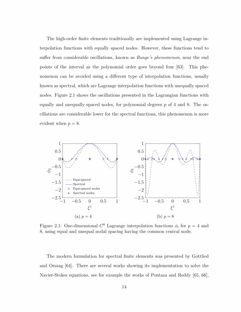
The high-order finite elements traditionally are implemented using Lagrange in-
terpolation functions with equally spaced nodes. However, these functions tend to
suffer from considerable oscillations, known as Runge’s phenomenon, near the end
points of the interval as the polynomial order goes beyond four [63]. This phe-
nomenon can be avoided using a different type of interpolation functions, usually
known as spectral, which are Lagrange interpolation functions with unequally spaced
nodes. Figure 2.1 shows the oscillations presented in the Lagrangian functions with
equally and unequally spaced nodes, for polynomial degrees p of 4 and 8. The os-
cillations are considerable lower for the spectral functions, this phenomenon is more
evident when p = 8.
−1 −0.5 0 0.5 1−2.5
−2
−1.5
−1
−0.5
0
0.5
1
ξ1
φ3
Equi-spaced
Spectral
Equi-spaced nodes
Spectral nodes
(a) p = 4
−1 −0.5 0 0.5 1−2.5
−2
−1.5
−1
−0.5
0
0.5
1
ξ1
φ5
(b) p = 8
Figure 2.1: One-dimensional C0 Lagrange interpolation functions φi for p = 4 and8, using equal and unequal nodal spacing having the common central node.
The modern formulation for spectral finite elements was presented by Gottlied
and Orszag [64]. There are several works showing its implementation to solve the
Navier-Stokes equations, see for example the works of Pontaza and Reddy [65, 66],
14
and Payette and Reddy [67]. The spectral functions have been also successfully used
to model shells by Zak and Krawczuk [68], Payette and Reddy [24], Gutierrez Rivera
and Reddy [27], and Gutierrez Rivera et al. [28].
Based on the advantages of the higher-order interpolation functions with un-
equally spaced nodes, the two shell finite elements developed in this dissertation are
modeled using them. In the following subsections, we present a general description
of these functions and important aspects about their implementation.
2.3.2 Implementation
Here, we recall some definitions and properties of spectral elements which are
crucial for the finite element formulations considered in this work. For a more detailed
presentation of these concepts, we refer to the text of Karniadakis and Sherwin [69].
The finite element implementations discussed here are based on the weak form
constructed using the Galerkin’s method. The weak statement can be expressed as
[70]: find u ∈ U such that
B(u,w) = L(w) ∀w ∈ W (2.11)
where B(u,w) is a bilinear form, L(w) is a linear form, and U and W are vector
spaces. The quantities u and w represent the set of dependent variables and testing
functions, respectively.
In order to solve the weak statement, we restrict the solution space of Equa-
tion 2.11 to a finite dimensional sub-space Uhp of the infinite dimensional space U
and the weighting function to a finite dimensional sub-space Whp ⊂ W . In the
15

discrete case, the weak form is stated as find uhp ∈ Uhp such that
B(uhp,whp) = L(whp) ∀whp ∈ Whp. (2.12)
The quantity h represents the average size of all the elements in the finite element dis-
cretization, while p denotes the polynomial degree of the finite element interpolation
functions associated with each element in the model.
Then, we assume that the domain Ω is discretized into a set of NE non-overlapping
finite elements Ωe, such that Ω ≈ Ωhp = ∪NEe=1Ωe. The geometry of each element is
characterized using the standard isoparametric bijective mapping from the master
element Ωe to the physical element Ωe [10]. For the shell elements presented here,
we observe that the shell mid-surface consist of a curved two-dimensional surface
embedded in a tree-dimensional space. For that reason, we can map the master ele-
ment Ωe = [−1,+1]2 in a two-dimensional manifold Ωe constituting the approximate
mid-surface of the eth element.
The dependent variables u are approximated using the general interpolation for-
mula
u(x) ≈ uhp(x) =n∑i=1
∆eiψi(ξ) in Ωe (2.13)
where ψi(ξ) are the 2-dimensional spectral interpolation functions, ∆ei is an array
containing the values of uhp(x) at the location of the ith node in Ωe, and n = (p+1)2
is the number of nodes in Ωe.
In order to construct the two-dimensional high-order interpolation functions, we
take the tensor product of the one-dimensional C0 spectral nodal basis φj, which are
16
given by
φj(ξ) =(ξ − 1)(ξ + 1)L′p(ξ)
p(p+ 1)Lp(ξj)(ξ − ξj)ξ ∈ [−1, 1] (2.14)
where Lp(ξ) is the Legendre polynomials of order p computed as
Lp(ξ) =(−1)p
2pp!
dp
dxp[(1− ξ)p(1 + ξ)p] ξ ∈ [−1, 1], (2.15)
and the quantities ξj are the locations of the nodes associated with the one-dimensional
interpolants. These nodes are known as the Gauss-Lobatto-Legendre points and are
computed by the roots of the following expression
(ξ − 1)(ξ + 1)L′p(ξ) = 0 ξ ∈ [−1, 1]. (2.16)
In this work, instead of using Equation 2.14 to construct the interpolation func-
tions, we use the traditional Lagrange formula
φj(ξ) =
p+1∏i=1i 6=j
(ξ − ξi)(ξj − ξi)
(2.17)
where ξi represent the location of the spectral nodes. The main reason is that this
expression is easier to implement in the finite element program. Also, the derivatives
of the one-dimensional spectral functions are computed in an simpler way, compared
to using Equation 2.14 to calculate them.
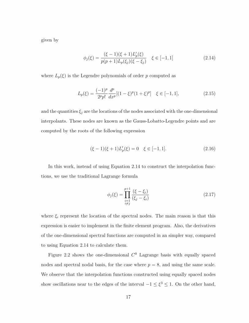
Figure 2.2 shows the one-dimensional C0 Lagrange basis with equally spaced
nodes and spectral nodal basis, for the case where p = 8, and using the same scale.
We observe that the interpolation functions constructed using equally spaced nodes
show oscillations near to the edges of the interval −1 ≤ ξ3 ≤ 1. On the other hand,
17
the spectral interpolation functions are free of the Runge’s phenomenon. Further-
more, the spectral nodal interpolation functions are known to be accurate and exhibit
exponential convergence [69]. For the reasons mentioned above, the finite element
coefficient matrices formulated with spectral basis functions are better conditioned,
which makes them yield accurate results [10].
The two-dimensional spectral bases can be obtained by taking the tensor product
of the one-dimensional spectral bases as
ψi(ξ1, ξ2) = φj(ξ
1)φk(ξ2) in Ωe (2.18)
where i = j + (k − 1)(p + 1) and j, k = 1, . . . , p + 1. Finite elements constructed
using these kind of interpolation functions are referred in the literature as spectral
elements [69]. Examples of these elements, for different p-levels are shown in Figure
2.3, where nodes are marked as . The node locations are calculated taking the
tensor product of the one-dimensional Gauss-Lobatto-Legendre points.
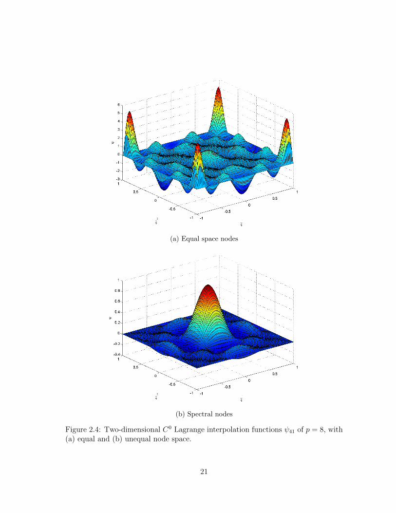
Figure 2.4 shows the two-dimensional interpolations functions using equal and
unequal spaced nodes at the central node (ξ1 = 0, ξ2 = 0). We observe considerable
oscillations for the first kind, near to the element corners, where the function ψ has a
higher value than one, approximately 5.38; while for the second one the oscillations
are less than one. This example clearly shows the advantage of the use of spectral
functions for the two dimensional domains studied in this dissertation.
Using the spectral functions previously defined, we substitute at element level
the approximate value of uhp, as well as the test function whp, into Equation (2.12),
in order to obtain a set of equations for the eth element in the form
[Ke]∆e = F e (2.19)
18

−1 −0.5 0 0.5 1−2.5
−2
−1.5
−1
−0.5
0
0.5
1
1.5
2
2.5
3
ξ3
φj
j = 1 j = 2 j = 3
j = 4 j = 5 j = 6
j = 7 j = 8 j = 9
(a) Equal space nodes
−1 −0.5 0 0.5 1−2.5
−2
−1.5
−1
−0.5
0
0.5
1
1.5
2
2.5
3
ξ3
φj
j = 1 j = 2 j = 3
j = 4 j = 5 j = 6
j = 7 j = 8 j = 9
(b) Spectral nodes
Figure 2.2: One-dimensional C0 Lagrange interpolation functions φj of p = 8, with(a) equal and (b) unequal node () space.
19

1
2
1 2 3
4 5 6
7 8 9
(a) 9-node element, p = 2
1
2
1 2 3 4 5
6 7 8 9 10
11 12 13 14 15
16 17 18 19 20
21 22 23 24 25
(b) 25-node element, p = 4
1
2
1 4 7
8 14
15 21
22 28
29 35
36 42
43 46 49
(c) 49-node element, p = 6
1
2
1 3 5 7 9
19 27
37 45
55 63
73 75 77 79 81
(d) 81-node element, p = 8
Figure 2.3: High-order spectral/hp quadrilateral master elements Ωe.
where [Ke] is the element coefficient matrix, ∆e is a vector containing the essential
variables at all the element nodes, and F e is the element force vector.
In this work, we utilize the standard Gauss-Legendre quadrature rules in the
numerical integration of all terms appearing in the element coefficient matrix and
force vector. We use full integration of all integrals in the coefficient matrix and force
vector. On the other hand, in the post-processing of the stresses, we employ reduced
integration points. The Gauss-Legendre quadrature weights wi are computed using
20
(a) Equal space nodes
(b) Spectral nodes
Figure 2.4: Two-dimensional C0 Lagrange interpolation functions ψ41 of p = 8, with(a) equal and (b) unequal node space.
21
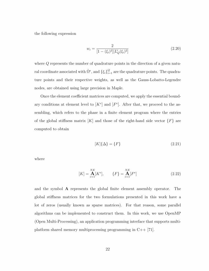
the following expression
wi =2
[1− (ξi)2][L′Q(ξi)2](2.20)
where Q represents the number of quadrature points in the direction of a given natu-
ral coordinate associated with Ωe, and ξiQi=1 are the quadrature points. The quadra-
ture points and their respective weights, as well as the Gauss-Lobatto-Legendre
nodes, are obtained using large precision in Maple.
Once the element coefficient matrices are computed, we apply the essential bound-
ary conditions at element level to [Ke] and [F e]. After that, we proceed to the as-
sembling, which refers to the phase in a finite element program where the entries
of the global stiffness matrix [K] and those of the right-hand side vector F are
computed to obtain
[K]∆ = F (2.21)
where
[K] =NE
Ae=1
[Ke], F =NE
Ae=1
[F e] (2.22)
and the symbol A represents the global finite element assembly operator. The
global stiffness matrices for the two formulations presented in this work have a
lot of zeros (usually known as sparse matrices). For that reason, some parallel
algorithms can be implemented to construct them. In this work, we use OpenMP
(Open Multi-Processing), an application programming interface that supports multi-
platform shared memory multiprocessing programming in C++ [71].
22

2.3.3 Static node condensation
In the high-order finite elements, the connectivity between the degrees of freedom
of a given element and also between neighboring elements increases with p. For that
reason, the higher-order finite elements require more computer memory resources to
store the global coefficient matrix, compared with the low-order finite elements with
the same number of degrees of freedom.
An efficient way to overcome this disadvantage is using element-level static con-
densation [69]. In order to perform this feature in our finite element formulations,
we reordered the equations at element level with respect to the degrees of freedom
at the boundary ∆eb and interior ∆e
i nodes, taking Equation 2.19 the following
form [Kebb] [Ke
bi]
[Keib] [Ke
ii]
∆
eb
∆ei
=
Feb
F ei
, (2.23)
or, if the block multiplications are made, can be expressed as
[Kebb]∆e
b+ [Kebi]∆e
i = F eb (2.24)
[Keib]∆e
b+ [Keii]∆e
i = F ei . (2.25)
We can solve for the interior degrees of freedom from Equation 2.25, to get
∆ei = [Ke
ii]−1F e
i − [Keii]−1[Ke
ib]∆eb. (2.26)
where its evident that the interior solution for each element does not have influ-
ence on the other element equations, and can be removed, substituting its value in
23
Equation 2.24 to get
[Ke]∆eb = F e (2.27)
where
[Ke] = [Kebb]− [Ke
bi][Keii]−1[Ke
ib] (2.28)
F e = F eb − [Ke
bi][Keii]−1F e
i . (2.29)
These terms can be evaluated efficiently using the dense matrix routines available in
LAPACK.
After the element equations with static condensed nodes are obtained, the equa-
tions are assembled as
[K]∆b = F (2.30)
where all the interior nodes have been removed. This leads to the solution for the
nodes at the element boundaries. For the interior degrees of freedom, those can be
obtained by solving the Equation 2.26 for each finite element.
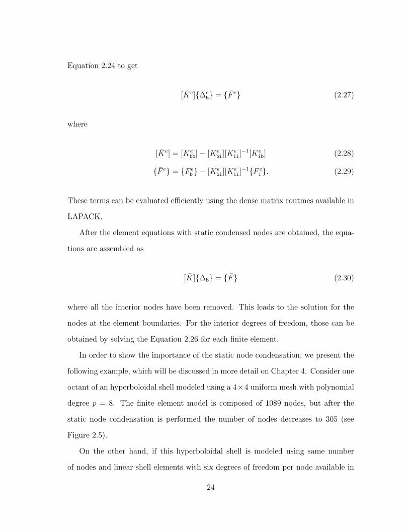
In order to show the importance of the static node condensation, we present the
following example, which will be discussed in more detail on Chapter 4. Consider one
octant of an hyperboloidal shell modeled using a 4×4 uniform mesh with polynomial
degree p = 8. The finite element model is composed of 1089 nodes, but after the
static node condensation is performed the number of nodes decreases to 305 (see
Figure 2.5).
On the other hand, if this hyperboloidal shell is modeled using same number
of nodes and linear shell elements with six degrees of freedom per node available in
24

(a) Total mesh (b) Statically condensed mesh
Figure 2.5: Mesh for an hyperboloidal shell using p = 8.
commercial codes (i.e. ABAQUS or ANSYS), the global stiffness matrix contains the
entrance for the total number of nodes. Even when the number of degrees of freedom
in the formulations presented here are larger than the ones in commercial codes, the
size of the matrix that should be inverted is lower for the formulations discussed here
(see Table 2.1 for details). The presented example shows how memory requirements
and the computational efficiency for the presented formulations are comparable to
lower-order shell finite elements.
Table 2.1: Comparison between the formulations presented and commercial codes.
Elements Total nodesStatic
condensed nodesStiffness
matrix size7-Parameter 16 1089 305 2135× 213512-Parameter 16 1089 305 3660× 3660Commercial codes 1024 1089 - 6534× 6534
25

3. EQUATIONS OF MOTION∗
In this section, we present and develop the equations of motion for the two models
used along this dissertation. The first model is based on an improved first-order shear
deformation theory with seven independent parameters. For that model, we use and
extend the seven-parameter continuum shell finite element formulation developed by
Payette and Reddy [24] to include thermal and transient analysis. The second one
has twelve independent parameters, which allow us to use the third-order thickness
stretching theory for static and transient analysis. Furthermore, the constitutive
equations and the procedure to compute the Cauchy stresses are presented.
The chapter is organized as follows. First, the procedure to parameterize the
three-dimensional geometry of the undeformed configuration of a typical shell ele-
ment is presented. The definitions of all the important terms for this task are also
presented, like the mid-surface approximation, the local basis vectors, and the co-
variant and contravariant basis vectors. After that, the displacement fields assumed
for the two formulations, and the procedure to compute the mechanical and thermal
strains are described. Later, the constitutive equations for the three materials consid-
ered in this investigation (isotropic, laminated composite and functionally graded)
are explained. Then, the procedure used to compute the Cauchy stress from the
second Piola–Kirchhoff stress is described. Finally, using these definitions, the equa-
tions of motion for the two formulations presented here are derived. In the following
discussions, we utilize the traditional convention where the Greek indices go from 1
to 2 while the Latin indices have the range of 1, 2, and 3.
∗Part of this chapter is reprinted with permission from “A new twelve-parameter spectral/hpshell finite element for large deformation analysis of composite shells” by M. Gutierrez Rivera, J.N. Reddy and M. Amabili, 2016. Composite Structures, Volume 151, pp. 183–196, Copyright 2016by Elsevier.
26
3.1 Parametrization of the shell
A finite element approximation of the mid-surface Ω is directly used and denoted
as Ωhp, with a set of NE high-order spectral/hp quadrilateral elements, and it is
represented by
Ωhp = ∪NEe=1Ωe. (3.1)
This leads to the following finite element approximation at element level:
X = φe(ξ1, ξ2) =n∑k=1
ψk(ξ1, ξ2)Xk, (3.2)
where X are the approximate mid-surface coordinates, ψk are the two-dimensional
spectral/hp basis functions associated with the kth node, n is the number of nodes
in the element, and Xk are the element nodal coordinates with respect to a fixed
orthogonal Cartesian coordinate system, with the basis vectors E1, E2, E3.
At each point of the mid-surface we compute the local basis vectors of the tangent
plane by means of the expression
aα =∂X
∂ξα≡ X,α (3.3)
and the unit normal vector as
a3 =a1 × a2
‖a1 × a2‖. (3.4)
However, instead of using a3, in this work we employ its finite element approximation
defined by
n =n∑k=1
ψk(ξ1, ξ2)nk (3.5)
27

where nk represents the nodal components of the unit normal to the shell mid-surface
with respect to a fixed orthogonal Cartesian coordinate system. Note that even when
we refer to n as unit normal, its magnitude differs slightly from one. For example,
the maximum difference in absolute value between the finite element approximation
for the spectral functions with p = 8 and one, at the full integration points, is equal
to 1.8794× 10⁻¹². However, these differences are negligible.
Using Equations (3.2) and (3.5), we can parameterize the three-dimensional ge-
ometry of the undeformed configuration of a typical shell element BR. The position
vector in the shell element can be described, assuming a constant thickness h, as
X = Φe(ξ1, ξ2, ξ3) = φe(ξ1, ξ2) + ξ3h
2n(ξ1, ξ2) (3.6)
where ξ3 ∈ [−1, 1]. This process is summarized in Figure 3.1, where the parent
element is mapped in to the mid-surface, and finally the physical element is recovered
using the normal and the shell thickness.
The covariant basis vectors at each point of the shell element are defined as
gi =∂X
∂ξi≡ X,i. (3.7)
Substituting the value of X from Equation (3.6) into Equation (3.7), we have
gα = aα + ξ3h
2n,α, g3 =
h
2n. (3.8)
In Figure 3.2 we present the vectors aα and gα at points A (at the middle surface)
and B (above A). Note that the local vectors of the tangent plane lie on the middle
surface (Ωe), while the covariant basis vectors are in a plane above it (Ωe∗).
The covariant vectors allow us to write a differential line element in the typical
28
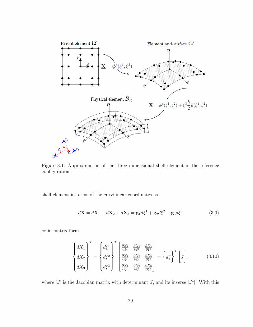
Figure 3.1: Approximation of the three dimensional shell element in the referenceconfiguration.
shell element in terms of the curvilinear coordinates as
dX = dX1 + dX2 + dX3 = g1dξ1 + g2dξ
2 + g3dξ3 (3.9)
or in matrix form
dX1
dX2
dX3
T
=
dξ1
dξ2
dξ3
T ∂X1
∂ξ1∂X2
∂ξ1∂X3
∂ξ1
∂X1
∂ξ2∂X2
∂ξ2∂X3
∂ξ2
∂X1
∂ξ3∂X2
∂ξ3∂X3
∂ξ3
=
dξ
T [J
], (3.10)
where [J ] is the Jacobian matrix with determinant J , and its inverse [J∗]. With this
29
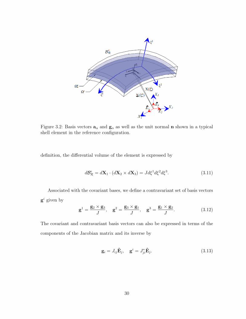
Figure 3.2: Basis vectors aα and gα as well as the unit normal n shown in a typicalshell element in the reference configuration.
definition, the differential volume of the element is expressed by
dBeR = dX1 · (dX2 × dX3) = Jdξ1dξ2dξ3. (3.11)
Associated with the covariant bases, we define a contravariant set of basis vectors
gi given by
g1 =g2 × g3
J, g2 =
g3 × g1
J, g3 =
g1 × g2
J. (3.12)
The covariant and contravariant basis vectors can also be expressed in terms of the
components of the Jacobian matrix and its inverse by
gi = JijEj, gi = J∗jiEj. (3.13)
30
3.2 Displacement fields
The displacement u of a material point X from the reference configuration to a
point x in the current configuration may be expressed as
u(X, t) = x(X, t)−X = χ(X, t)−X, (3.14)
where χ(X, t) represents the mapping of the shell from the reference to the current
configuration. The displacement vector at any point within the shell element can be
approximated by a Taylor series expansion with respect to the curvilinear thickness
coordinate ξ3 as
u(X(ξi), t) =∞∑k=1
(ξ3)k
k!u(k)(ξα, t) |ξ3=0
= u(0)(ξα, t) + ξ3u(1)(ξα, t) +(ξ3)2
2u(2)(ξα, t) + · · · , (3.15)
where u(k)(ξα, t) = ∂ku(ξi, t)/∂(ξ3)k |ξ3=0. If an infinite number of terms is used, the
exact motion of the three-dimensional body is recovered (see Naghdi [72]).
In this work, we truncate the Taylor series to use three-dimensional elasticity and
three-dimensional constitutive relations. As a function of the number of parameters
used, two different formulations with different order of approximation are obtained.
These have seven and twelve independent parameters, in order to avoid spurious
stresses in the thickness direction presented in the six-parameter formulation (nor-
mally referred to as Poisson locking [51]). Note that this kind of locking cannot be
avoided with mesh refinement, since the stiffening process comes from the theory and
not from the numerical approximation. General details are described in the following
subsections.
31
3.2.1 Seven-parameter formulation
In this case, we assume that the displacement field is a linear expansion of the
thickness coordinate around the mid-surface, and the transverse displacement is
parabolic through the thickness of the shell [22]. These assumptions give the fol-
lowing seven-parameter expansion
u(ξi, t) = u(ξα, t) + ξ3h
2ϕ(ξα, t) + (ξ3)2h
2Ψ(ξα, t) (3.16)
where we rename each u(j)(ξα, t), for j = 0, 1, 2, by some variables and scale the last
two by a factor of h/2. These new variables can be expressed as
u(ξα, t) = ui(ξα, t)Ei, ϕ(ξα, t) = ϕi(ξ
α, t)Ei, Ψ(ξα, t) = Ψ(ξα, t)n(ξα). (3.17)
Here u denotes the mid-plane displacement vector, ϕ is the difference vector and it
gives the change in the mid-surface director, and Ψ is the vector with one component
(namely the seventh parameter) that is used to circumvent the Poisson locking.
The position vector at each load step can be obtained substituting Equations
(3.6) and (3.16) into (3.14), to obtain
x = (X + u) + ξ3h
2(n +ϕ) + (ξ3)2h
2Ψn
= x + ξ3h
2n + (ξ3)2h
2Ψn. (3.18)
where the terms x and n represent the location of a point on the deformed mid-
surface and the director of the deformed mid-surface, respectively. Note that n is
not normal to the deformed mid-surface.
32
3.2.2 Twelve-parameter formulation
For this formulation, we truncate the Taylor series up to cubic terms, making the
displacement field a function of twelve independent parameters, and a cubic expan-
sion of the thickness coordinate around the mid-surface and through the thickness
of the shell. This displacement field is analogous to the one proposed by Amabili
[25, 26] for double curved shells. In these works, he imposed zero shear stress at the
top and bottom surfaces to reduce the number of parameters in his formulation to
only eight. However, we avoid this approach, since the resulting number of terms
in the tangent matrix (details about how to obtain it can be found in Chapter 4)
is in the order of millions, and the use of C1 continuity functions is required. The
displacement field with twelve independent parameters allows the use of C0 conti-
nuity functions and reduces considerably the number of terms in the tangent matrix
to only 73476, for shells under mechanical loads. The twelve-parameter expansion
considered in this work is expressed as
u(ξi, t) = u(ξα, t) + ξ3h
2ϕ(ξα, t) + (ξ3)2h
2Ψ(ξα, t) + (ξ3)3h
2Θ(ξα, t) (3.19)
where each u(j)(ξα, t), for j = 0, 1, 2, 3, has been renamed by some variables and the
last three have been scaled by a factor of h/2. These new variables can be expressed
as
u(ξα, t) = ui(ξα, t)Ei, ϕ(ξα, t) = ϕi(ξ
α, t)Ei, (3.20)
Ψ(ξα, t) = Ψi(ξα, t)Ei, Θ(ξα, t) = Θi(ξ
α, t)Ei.
Here u and ϕ have the same meaning as they have in the seven-parameter expansion.
Now, Ψ and Θ are vectors with three components used to circumvent the spurious
33
stresses in the thickness direction presented in a six parameter formulation. Note
that even when Ψ is also used in the seven-parameter formulation, the meaning is
different.
The position vector at each load step can be constructed by substituting Equa-
tions (3.6) and (3.19) into (3.14), which results in
x = (X + u) + ξ3h
2(n +ϕ) + (ξ3)2h
2Ψ + (ξ3)3h
2Θ
= x + ξ3h
2n + (ξ3)2h
2Ψ + (ξ3)3h
2Θ. (3.21)
Here the terms u and ϕ have the same meaning as in the seven-parameter formula-
tion.
3.3 Mechanical strains
Strains measure the relative displacement of material elements within a body.
Different measures for the mechanical strains are encountered in the literature. For
small deformations, the traditional Cauchy strain is used. However, when defor-
mations are large other measures of strains are needed, like the Green–Lagrange,
Almansi-Hamel and Hencky strains [73]. A general description of these strains is
given for the unidirectional case to bring out the general differences.
Consider the axial deformation of an isotropic bar, which is stress free at the
reference configuration. This deformation can be represented using the stretch ratio
λa, defined as the current length l, divided by the length at the reference configuration
lR
λa =l
lR. (3.22)
This quantity is used to compute different measures of strain.
34
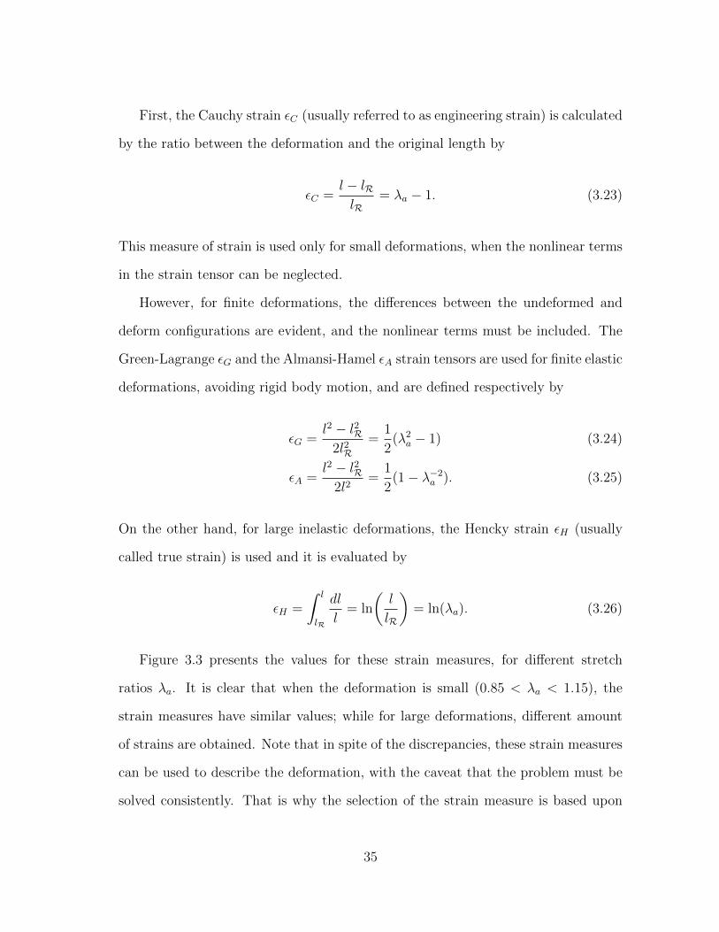
First, the Cauchy strain εC (usually referred to as engineering strain) is calculated
by the ratio between the deformation and the original length by
εC =l − lRlR
= λa − 1. (3.23)
This measure of strain is used only for small deformations, when the nonlinear terms
in the strain tensor can be neglected.
However, for finite deformations, the differences between the undeformed and
deform configurations are evident, and the nonlinear terms must be included. The
Green-Lagrange εG and the Almansi-Hamel εA strain tensors are used for finite elastic
deformations, avoiding rigid body motion, and are defined respectively by
εG =l2 − l2R
2l2R=
1
2(λ2
a − 1) (3.24)
εA =l2 − l2R
2l2=
1
2(1− λ−2
a ). (3.25)
On the other hand, for large inelastic deformations, the Hencky strain εH (usually
called true strain) is used and it is evaluated by
εH =
∫ l
lR
dl
l= ln
(l
lR
)= ln(λa). (3.26)
Figure 3.3 presents the values for these strain measures, for different stretch
ratios λa. It is clear that when the deformation is small (0.85 < λa < 1.15), the
strain measures have similar values; while for large deformations, different amount
of strains are obtained. Note that in spite of the discrepancies, these strain measures
can be used to describe the deformation, with the caveat that the problem must be
solved consistently. That is why the selection of the strain measure is based upon
35

its intended use.
0.5 1 1.5 2−1.5
−1
−0.5
0
0.5
1
1.5
Stretch ratio λa
Str
ain
Cauchy
Green–Lagrange
Almansi-Hamel
Hencky
Figure 3.3: Strain measures versus stretch ratio.
The extension of the presented measures of strain to the three dimensional case
can be found in the text of Truesdell [74]. In this work, we assume that all the
kinematic variables are referred to the initial configuration (Lagrangian description)
and only finite elastic deformations will be studied. For that reason, we choose
the Green–Lagrange strain tensor. General details on how to implement this strain
measure for shells are presented in the following lines.
First, the deformation gradient F should be computed by [75]
F = ∇0χ(X, t) = ∇0(X + u) = I +∇0u (3.27)
where the symbol ∇0 denotes the material gradient operator relative to the reference
configuration. The identity tensor can be expressed as I = gi⊗gi and ∇0u = u,i⊗gi
36
(see the text of Basar and Weichert [76] for details). Equation (3.27) becomes
F = gi ⊗ gi + u,i ⊗ gi
= (gi + u,i)⊗ gi. (3.28)
Once the deformation gradient is computed, the Green–Lagrange strain tensor E
is obtained by
E =1
2(FTF− I)
=1
2(u,i · gj + gi · u,j + u,i · u,j)gi ⊗ gj. (3.29)
The covariant components of the tensor E can be expanded as a function of the
thickness coordinate ξ3 as
Eij(ξm, t) =ε(0)(ξα, t) + ξ3ε(1)(ξα, t) + (ξ3)2ε(2)(ξα, t) + (ξ3)3ε(3)(ξα, t) (3.30)
+ (ξ3)4ε(4)(ξα, t),
for the seven-parameter formulation; while for the twelve-parameter they become
Eij(ξm, t) =ε(0)(ξα, t) + ξ3ε(1)(ξα, t) + (ξ3)2ε(2)(ξα, t) + (ξ3)3ε(3)(ξα, t) (3.31)
+ (ξ3)4ε(4)(ξα, t) + (ξ3)5ε(5)(ξα, t) + (ξ3)6ε(6)(ξα, t).
In this work we neglect, for simplicity but without loss of engineering accuracy,
all the quadratic and higher-order terms of the covariant components of the Green–
Lagrange strain tensor E for the seven-parameter formulation. The retained covari-
37
ant components may be determined as
ε(0)αβ =
1
2
(u,α · aβ + aα · u,β + u,α · u,β
)(3.32)
ε(1)αβ =
h
4
(u,α · (n,β +ϕ,β) + (n,α +ϕ,α) · u,β +ϕ,α · aβ + aα ·ϕ,β
)(3.33)
ε(0)α3 =
h
4
[u,α · (n +ϕ) + aα ·ϕ
](3.34)
ε(1)α3 =
h
2
h
4
[ϕ,α · n + (n,α +ϕ,α) ·ϕ
]+ (aα + u,α) ·Ψ
(3.35)
ε(0)33 =
h2
8
(2n +ϕ
)·ϕ (3.36)
ε(1)33 =
h2
2
(n +ϕ
)·Ψ. (3.37)
Note that if the seven parameter Ψ is set to zero, we obtain the six parameter
formulation with zero transverse strain ε(1)33 .
For the twelve-parameter formulation, we neglect all the cubic and higher-order
terms of the covariant components of the Green–Lagrange strain tensor E, in order
to recover the twelve parameters presented and to obtain a quadratic distribution of
the transverse strains. The retained covariant components may be determined using
Equations (3.32)-(3.37), and the additional therms are computed using
ε(2)αβ =
h
4
h
2
[ϕ,α · n,β + n,α ·ϕ,β +ϕ,α ·ϕ,β
]+ Ψ,α · (u,β + aβ) + (u,α + aα) ·Ψ,β
(3.38)
ε(2)α3 =
h
8
h
[Ψ,α · (n +ϕ) + 2(n,α +ϕ,α) ·Ψ
]+ 6(aα + u,α) ·Θ
(3.39)
ε(2)33 =
h2
4
[3(n +ϕ) ·Θ + 2Ψ ·Ψ
]. (3.40)
Note that, even when Equations (3.32)-(3.37) are the same as the seven-parameter
38

formulation, the definition of Ψ is different.
3.4 Thermal strains
In some applications, in addition to the mechanicals loads, the shell structures
can be exposed to thermal loads. In this work, we develop the thermoelastic analysis
based on the multiplicative decomposition proposed by Stojanovitch et al. [77],
and then present some assumptions to arrive to the linearized form used along this
dissertation. General aspects for the multiplicative decomposition are presented and
a more detailed explanation can be found in the paper by Vujosevic and Lubarda
[78].
The thermoelastic material response is based on the introduction of an inter-
mediate configuration Bθ between the reference configuration BR and the current
configuration B. The thermal deformation gradient from BR to Bθ is denoted by Fθ,
and the isothermal elastic deformation gradient from Bθ to B is denoted by Fe. The
total deformation gradient F is decomposed as
F = Fe · Fθ. (3.41)
The elastic Lagrangian strain EL for thermal analysis can be computed by
EL = FTθ · Ee · Fθ + Eθ, (3.42)
where the elastic Ee and thermal Eθ strain tensors are defined as
Ee =1
2(FT
e · Fe − I) (3.43)
Eθ =1
2(FT
θ · Fθ − I). (3.44)
39
The thermal deformation gradient Fθ is defined, for isotropic materials, by
Fθ = ϑ(θ)I (3.45)
where ϑ(θ) is the thermal stretch ratio in an arbitrary direction. The relation between
the thermal stretch ratio and the coefficient of thermal expansion α is given by
α(θ) =1
ϑ
dϑ
dθ. (3.46)
Integrating the previous expression from the reference temperature at which the shell
is stress free T0 to the current temperature T , and assuming that the properties are
not function of the temperature it gives
ϑ(θ) = exp
[ ∫ T
T0
αdθ
]= exp[α(T − T0)]. (3.47)
In this work, the influence of the temperature is studied only for isotropic func-
tionally graded materials. Also it is assumed that there is only variation of the
temperature through the thickness of the shell, and the product α(T −T0) 1. The
last assumption allows us to linearize the thermal strain Eθ, that will be distinguished
using the notation ε(T ), and it is given by
ε(T )(ξ3) = α(ξ3)∆T (ξ3) (3.48)
where α(ξ3) is the second order tensor of the coefficients of thermal expansion of the
material, and ∆T (ξ3) = T (ξ3)− T0 is the increment of temperature. In an arbitrary
40
curvilinear system, the covariant components of Equation (3.48) can be obtained by
ε(T )ij (ξ3) = α(ξ3)gij∆T (ξ3) (3.49)
where gij are the covariant components of the Riemannian metric tensor G in the
reference configuration.
3.5 Stresses and constitutive equations
Since in this work only the mechanical response for elastic shells is studied, we
assume that the relation between the second Piola–Kirchhoff stress tensor S with the
Green–Lagrange strain tensor E and the linearized thermal strains ε(T ) is described
by
S = C(E− ε(T )), (3.50)
where C = Cijklgi⊗gj ⊗gk⊗gl is the fourth-order elasticity tensor, and we assume
that it is independent of the shell deformation and the temperature. Note that, in
general, the elasticity tensor has 81 components. However, due to the symmetry of
the stress and strain tensor the number of therms is reduced to 36, and due to the
assumption that the material is hyperelastic (the existence of a strain energy density
function) the number of independent elastic component is reduced to 21 (for details
see the text of Sadd [79]).
The contravariant components of S may be determined as
Sij = Cijkl(Ekl − ε(T )kl ) (3.51)
and the second Piola–Kirchhoff stress tensor S can be expressed as
S = Sijgi ⊗ gj. (3.52)
41
The physical components of S with respect to the basis Ei ⊗ Ej can be defined as
Sij = Skl(gk · Ei)(gl · Ej). (3.53)
Note that in the above equation the term Sij refers to the physical (as opposed to
the covariant) components.
Finally, the Cauchy stress tensor can be obtained from the second Piola–Kirchhoff
stress tensor S using the relation (see Reddy [75])
σ =1
det(F)F · S · FT (3.54)
where F refers to the deformation gradient, previously defined in Equation (3.28).
However, these components should be transformed to the fixed Cartesian coordinate
system by
Fij = Ei · FEj (3.55)
giving the physical components of F to be used in Equation (3.54). Again, note
that in the above equation Fij refers to the physical (as opposed to the covariant)
components of F.
3.5.1 Homogeneous isotropic shells
Isotropic shells are highly used in engineering; structures made with steel like
pressure vessels, large roofs or the bodies of automobiles are some examples. For
these materials, only two constants are needed in order to compute the fourth-order
elasticity tensor C, and its contravariant components are [1]
Cijkl = λgijgkl + µ(gikgjl + gilgjk), (3.56)
42
where λ and µ are the Lame parameters, and they can be expressed as
λ =νE
(1 + ν)(1− 2ν), µ =
E
2(1 + ν). (3.57)
Also, in Equation (3.56), gij = gi · gj are the contravariant components of the Rie-
mannian metric tensor G in the reference configuration. Even though the elasticity
tensor is only function of the Lame parameters, its 21 components are in general
different from each other.
3.5.2 Functionally graded shells
Functionally graded materials were originated in the mid 1980s by a group of
scientists in Japan [80, 81]. These materials are made from different phases of mate-
rial constituents (e.g., ceramic and metal for thermal barrier structures), and their
mechanical properties vary smoothly and continuously from one point to another,
eliminating the interface problems and mitigating stress concentrations.
For a two-constituent functionally graded through the thickness shell, we assume
that Poisson’s ratio ν is constant and the other properties (Young’s modulus E,
coefficient of thermal expansion α, thermal conductivity K, and density ρ) vary
through the thickness coordinate ξ3 according to the power-law (see Praveen and
Reddy [82])
P (ξ3) = (P+ − P−)f+(ξ3) + P− (3.58)
where
f+(ξ3) =(ξ3 + 1
2
)n. (3.59)
The quantities P+ and P− represent properties at the top (+) and bottom (-) sur-
faces, respectively. In this work, we assume that the bottom surface is 100% metal
and the top surface is 100% ceramic, and that these properties are temperature in-
43
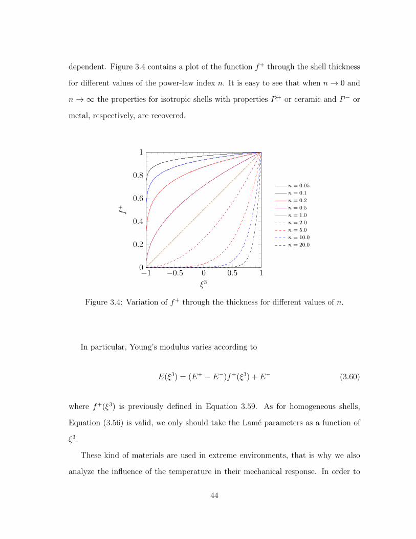
dependent. Figure 3.4 contains a plot of the function f+ through the shell thickness
for different values of the power-law index n. It is easy to see that when n→ 0 and
n →∞ the properties for isotropic shells with properties P+ or ceramic and P− or
metal, respectively, are recovered.
−1 −0.5 0 0.5 10
0.2
0.4
0.6
0.8
1
ξ3
f+
n = 0.05
n = 0.1
n = 0.2
n = 0.5
n = 1.0
n = 2.0
n = 5.0
n = 10.0
n = 20.0
Figure 3.4: Variation of f+ through the thickness for different values of n.
In particular, Young’s modulus varies according to
E(ξ3) = (E+ − E−)f+(ξ3) + E− (3.60)
where f+(ξ3) is previously defined in Equation 3.59. As for homogeneous shells,
Equation (3.56) is valid, we only should take the Lame parameters as a function of
ξ3.
These kind of materials are used in extreme environments, that is why we also
analyze the influence of the temperature in their mechanical response. In order to
44
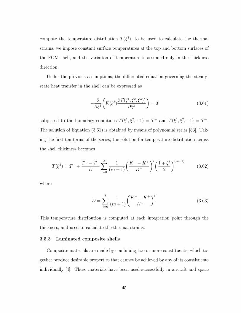
compute the temperature distribution T (ξ3), to be used to calculate the thermal
strains, we impose constant surface temperatures at the top and bottom surfaces of
the FGM shell, and the variation of temperature is assumed only in the thickness
direction.
Under the previous assumptions, the differential equation governing the steady-
state heat transfer in the shell can be expressed as
− ∂
∂ξ3
(K(ξ3)
∂T (ξ1, ξ2, ξ3))
∂ξ3
)= 0 (3.61)
subjected to the boundary conditions T (ξ1, ξ2,+1) = T+ and T (ξ1, ξ2,−1) = T−.
The solution of Equation (3.61) is obtained by means of polynomial series [83]. Tak-
ing the first ten terms of the series, the solution for temperature distribution across
the shell thickness becomes
T (ξ3) = T− +T+ − T−
D
8∑i=0
1
(in+ 1)
(K− −K+
K−
)i(1 + ξ3
2
)(in+1)
(3.62)
where
D =8∑i=0
1
(in+ 1)
(K− −K+
K−
)i. (3.63)
This temperature distribution is computed at each integration point through the
thickness, and used to calculate the thermal strains.
3.5.3 Laminated composite shells
Composite materials are made by combining two or more constituents, which to-
gether produce desirable properties that cannot be achieved by any of its constituents
individually [4]. These materials have been used successfully in aircraft and space
45
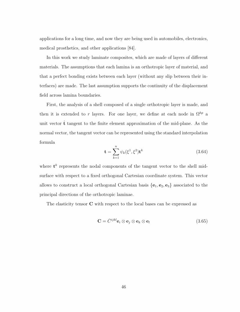
applications for a long time, and now they are being used in automobiles, electronics,
medical prosthetics, and other applications [84].
In this work we study laminate composites, which are made of layers of different
materials. The assumptions that each lamina is an orthotropic layer of material, and
that a perfect bonding exists between each layer (without any slip between their in-
terfaces) are made. The last assumption supports the continuity of the displacement
field across lamina boundaries.
First, the analysis of a shell composed of a single orthotropic layer is made, and
then it is extended to r layers. For one layer, we define at each node in Ωhp a
unit vector t tangent to the finite element approximation of the mid-plane. As the
normal vector, the tangent vector can be represented using the standard interpolation
formula
t =n∑k=1
ψk(ξ1, ξ2)tk (3.64)
where tk represents the nodal components of the tangent vector to the shell mid-
surface with respect to a fixed orthogonal Cartesian coordinate system. This vector
allows to construct a local orthogonal Cartesian basis e1, e2, e3 associated to the
principal directions of the orthotropic laminae.
The elasticity tensor C with respect to the local bases can be expressed as
C = Cijklei ⊗ ej ⊗ ek ⊗ el (3.65)
46

where the components of Cijkl in matrix form are
[Cijkl
]=
C1111 C1122 C1133 0 0 0
C1122 C2222 C2233 0 0 0
C1133 C2233 C3333 0 0 0
0 0 0 C2323 0 0
0 0 0 0 C1313 0
0 0 0 0 0 C1212
, (3.66)
or, as a function of the nine independent engineering elastic constants: E1, E2, E3,
ν12, ν13, ν23, G12, G13 and G23, as
[Cijkl
]=
1E1
−ν12E1−ν13
E10 0 0
−ν12E1
1E2
−ν23E2
0 0 0
−ν13E1−ν23
E2
1E3
0 0 0
0 0 0 1G23
0 0
0 0 0 0 1G13
0
0 0 0 0 0 1G12
−1
. (3.67)
Also, the local bases for the principle directions of the material in Equation (3.65)
are given by
e1 = t cos(θ) + n× t sin(θ)
e2 = −t sin(θ) + n× t cos(θ)
e3 = n (3.68)
where θ is the angle of rotation of the tangent t about the normal n.
47

The contravariant components of the elastic tensor C can be obtained contracting
Equation (3.65) with gi ⊗ gj ⊗ gk ⊗ gl which gives
Cijkl = TimTjnTkpTlqCmnpq (3.69)
where the components of Tij are
Tij = gi · ej. (3.70)
Note that Equation 3.69 has five matrix multiplication that result in the 21 indepen-
dent components in Cijkl.
Now, for multi-layered composites, in addition to the tangent vector t a set of
orientation angles associated with each ply θ = (θ1, ..., θNL) must be defined, where
NL is the number of layers. These layers are numbered from the bottom to the top
ply. At any arbitrary layer r the local material vectors er1, er2, er3 are obtained using
θr instead of θ in Equation (3.68). After that, the components of Cijkl in the rth
layer are determined using Equation (3.69).
3.6 Equations of motion
The governing equations of the shell models are derived, using the displacement
fields of Equations (3.16) and (3.19), by means of Hamilton’s principle (see Reddy
[85]). This principle is stated as
∫ T
0
δLdt ≡∫ T
0
[δK − (δU + δV )]dt = 0 (3.71)
48

where δK denotes the virtual kinetic energy, δU the virtual strain energy, and δV
the virtual potential energy due to the applied loads. These terms can be defined as
δK =
∫B0δu · ρ0udB0 (3.72)
δU =
∫B0δE · SdB0 (3.73)
δV = −∫B0δu · ρ0b0dB0 −
∫Γσ
δu · t0ds, (3.74)
where ρ0 is the density, b0 is the body force vector, and t0 is the traction vector, all
expressed and measured with respect to the undeformed configuration.
For the seven-parameter formulation, Equations (3.72 - 3.74) become
δK =
∫Ω
∫ 1
−1
ρ0
(ui + ξ3h
2ϕi + (ξ3)2h
2Ψni
)(δui + ξ3h
2δϕi + (ξ3)2h
2δΨni
)Jdξ3dΩ
=
∫Ω
[I0
(uiδui
)+ I1
h
2
(uiδϕi + ϕiδui
)+ I2
h
2
(Ψδuini + uiδΨni +
h
2ϕiδϕi
)+ I3
(h
2
)2(Ψδϕini + ϕiδΨni
)+ I4
(h
2
)2
ΨδΨ‖n‖]dΩ (3.75)
δU =
∫Ω
∫ 1
−1
(δε(0)ij + ξ3δε
(1)ij )Cijkl(ε
(0)kl + ξ3ε
(1)kl − ε
(T ))Jdξ3dΩ
=
∫Ω
[Aijklδε
(0)ij ε
(0)kl +Bijkl
(δε
(0)ij ε
(1)kl + δε
(1)ij ε
(0)kl
)+Dijklδε
(1)ij ε
(1)kl
+ Aijkl(T )δε(0)ij gkl +Bijkl(T )δε
(1)ij gkl
]dΩ (3.76)
δV =−∫B0
(δu + ξ3h
2δϕ+ (ξ3)2h
2δΨ
)· ρ0b0dB0
−∫
Γσ
(δu + ξ3h
2δϕ+ (ξ3)2h
2δΨ
)· t0ds, (3.77)
49

while for the twelve-parameter formulation are
δK =
∫Ω
∫ 1
−1
ρ0
(ui + ξ3h
2ϕi + (ξ3)2h
2Ψ + (ξ3)3h
2Θ
)(δui + ξ3h
2δϕi + (ξ3)2h
2δΨ + (ξ3)3h
2δΘ
)Jdξ3dΩ
=
∫Ω
[I0
(uiδui
)+ I1
h
2
(uiδϕi + ϕiδui
)+ I2
h
2
(uiδΨi + Ψiδui +
h
2ϕiδϕi
)+ I3
h
2
(uiδΘi + Θiδui +
h
2Ψiδϕi +
h
2ϕiδΨi
)+ I4
(h
2
)2(ϕiδΘi + Θiδϕi + ΨiδΨi
)+ I5
(h
2
)2(ΨiδΘi + ΘiδΨi
)+ I6
(h
2
)2(ΘiδΘi
)]dΩ (3.78)
δU =
∫Ω
∫ 1
−1
(δε(0)ij + ξ3δε
(1)ij + (ξ3)2δε
(2)ij )
Cijkl(ε(0)kl + ξ3ε
(1)kl + (ξ3)2ε
(2)kl − ε
(T ))Jdξ3dΩ
=
∫Ω
[Aijklδε
(0)ij ε
(0)kl +Bijkl
(δε
(0)ij ε
(1)kl + δε
(1)ij ε
(0)kl
)+Dijkl(δε
(0)ij ε
(2)kl + δε
(1)ij ε
(1)kl + δε
(2)ij ε
(0)kl )
+ Eijkl(δε
(1)ij ε
(2)kl + δε
(2)ij ε
(1)kl
)+Gijklδε
(2)ij ε
(2)kl
+ Aijkl(T )δε(0)ij gkl +Bijkl(T )δε
(1)ij gkl +Dijkl(T )δε
(2)ij gkl
]dΩ (3.79)
δV =−∫B0
(δu + ξ3h
2δϕ+ (ξ3)2h
2δΨ + (ξ3)3h
2δΘ
)· ρ0b0dB0
−∫
Γσ
(δu + ξ3h
2δϕ+ (ξ3)2h
2δΨ + (ξ3)3h
2δΘ
)· t0ds, (3.80)
where ‖ · ‖ denotes the Euclidean norm, Ii are the mass inertias defined by
Ii =
∫ 1
−1
ρ0(ξ3)iJdξ3 (i = 0, 1, 2, 3, 4, 5, 6), (3.81)
50
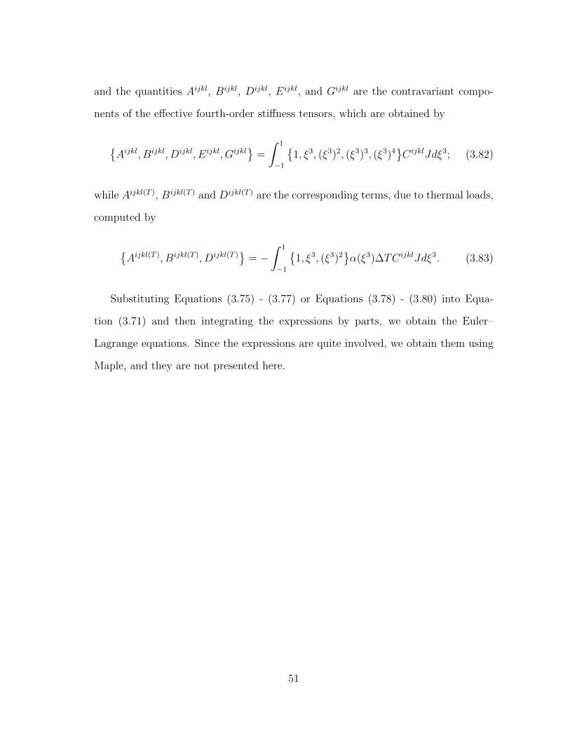
and the quantities Aijkl, Bijkl, Dijkl, Eijkl, and Gijkl are the contravariant compo-
nents of the effective fourth-order stiffness tensors, which are obtained by
Aijkl, Bijkl, Dijkl, Eijkl, Gijkl
=
∫ 1
−1
1, ξ3, (ξ3)2, (ξ3)3, (ξ3)4
CijklJdξ3; (3.82)
while Aijkl(T ), Bijkl(T ) and Dijkl(T ) are the corresponding terms, due to thermal loads,
computed by
Aijkl(T ), Bijkl(T ), Dijkl(T )
= −
∫ 1
−1
1, ξ3, (ξ3)2
α(ξ3)∆TCijklJdξ3. (3.83)
Substituting Equations (3.75) - (3.77) or Equations (3.78) - (3.80) into Equa-
tion (3.71) and then integrating the expressions by parts, we obtain the Euler–
Lagrange equations. Since the expressions are quite involved, we obtain them using
Maple, and they are not presented here.
51
4. STATIC ANALYSIS∗
In this chapter, the finite element models, for the static analysis of the nonlinear
shell formulations described in Chapter 3, are developed using the principle of virtual
displacements to obtain the weak form. The resulting equations are linearized, and
the discrete tangent operator is obtained. The discretization of the displacement
fields is also presented. The nonlinear systems of algebraic equations are solved by
means of incremental iterative methods. In particular, Newton’s method and the arc-
length method are used, and details about their implementation for the formulations
discussed in this dissertation are presented.
Numerical results for different benchmark problems are introduced, to prove
the advantages of the presented formulations. First, we compare with some semi-
analytical solutions for isotropic plates and shells obtained using higher-order shear
deformation theories available in the literature. Later, we contrast some experi-
mental data for laminated composite materials under large deformation with the
displacements predicted by means of the present formulations. After that, we show
a comparison with analytical solutions for functionally graded materials. Also, the
advantages of the present formulations, compared with the three dimensional solid
elements used in commercial codes, for thermo-mechanical analysis are presented.
Finally, we solve ten benchmark problems presented in the literature. For some of
them, the material properties, geometries and/or loads listed in the references are
∗Part of this chapter is reprinted with permission from “Stress analysis of func-tionally graded shells using a 7-parameter shell element” by M. Gutierrez Riveraand J. N. Reddy, 2016. Mechanics Research Communications, available online:http://www.sciencedirect.com/science/article/pii/S0093641316000343, Copyright 2016 by El-sevier, and from “A new twelve-parameter spectral/hp shell finite element for large deformationanalysis of composite shells” by M. Gutierrez Rivera, J. N. Reddy and M. Amabili, 2016. CompositeStructures, Volume 151, pp. 183–196, Copyright 2016 by Elsevier.
52

changed, to give a more realistic approach to these problems. Furthermore, some of
these benchmark problems are solved using the linear shell elements available in the
commercial codes ANSYS and ABAQUS to bring out the differences.
4.1 Finite element model
The finite element models presented are based on the assumption that the mid-
surface is discretized into NE non overlapping elements, as described in Chapter 3.
Furthermore, the displacement fields presented are interpolated using different finite
element approximations. For the the seven-parameter formulation this is given by
u(ξi, t) =n∑k=1
ψk(ξ1, ξ2)
[uk(t) + ξ3h
2ϕk(t) + (ξ3)2h
2Ψk(t)n(ξα)
](4.1)
where the normal n is computed using Equation (3.5) and Ψk(t) is interpolated
separately in this approximation. The derivatives of the above displacement field are
computed using
u,α(ξi, t) =n∑k=1
∂ψk∂ξα
[uk(t) + ξ3h
2ϕk(t) + (ξ3)2h
2
(Ψk(t)n(ξβ) + nkΨ(ξβ, t)
)](4.2)
u,3(ξi, t) = hn∑k=1
ψk(ξ1, ξ2)
[1
2ϕk(t) + ξ3Ψk(t)n(ξβ)
]. (4.3)
On the other hand, the displacement field assumed for the twelve-parameter formu-
lation is approximated by
u(ξi, t) =n∑k=1
ψk(ξ1, ξ2)
[uk(t) + ξ3h
2ϕk(t) + (ξ3)2h
2Ψk(t) + (ξ3)3h
2Θk(t)
](4.4)
where the use of the normal is avoided and all the components of the displacement are
interpolated up to cubic terms with respect to the thickness coordinate. This time,
53

the derivatives of the displacement field with respect to the curvilinear coordinates
are given by
u,α(ξi, t) =n∑k=1
∂ψk∂ξα
[uk(t) + ξ3h
2ϕk(t) + (ξ3)2h
2Ψk(t) + (ξ3)3h
2Θk(t)
](4.5)
u,3(ξi, t) = hn∑k=1
ψk(ξ1, ξ2)
[1
2ϕk(t) + ξ3Ψk(t) + (ξ3)2 3
2Θk(t)
]. (4.6)
The six Equations previously defined are used to solve the static and transient anal-
ysis of the shell formulations presented, as will be discussed in this and the next
Chapter.
In order to solve the static analysis we use the principle of virtual displacements
(the static version of Hamilton’s principle). This principle can be stated as follows:
the total virtual work done by actual internal (δU) as well as external (δV ) forces in
moving through their respective virtual displacements is zero. For this continuous
problem, the following weak statement holds:
G(δΦ,Φ) = δU(δΦ,Φ) + δV (δΦ,Φ) ≡ 0, (4.7)
where the terms δU and δV are defined by Eqs. (3.73) and (3.74), respectively.
We apply Newton’s method and the cylindrical arc-length method [36] to solve the
resulting nonlinear set of algebraic equations. The general aspects are presented in
the following subsections.
4.1.1 Newton’s method
The solution to the nonlinear equations found using the principle of the virtual
displacements can be obtained by means of the Newton’s method. This process
generally involves the linearization of the equilibrium equations, using the directional
54
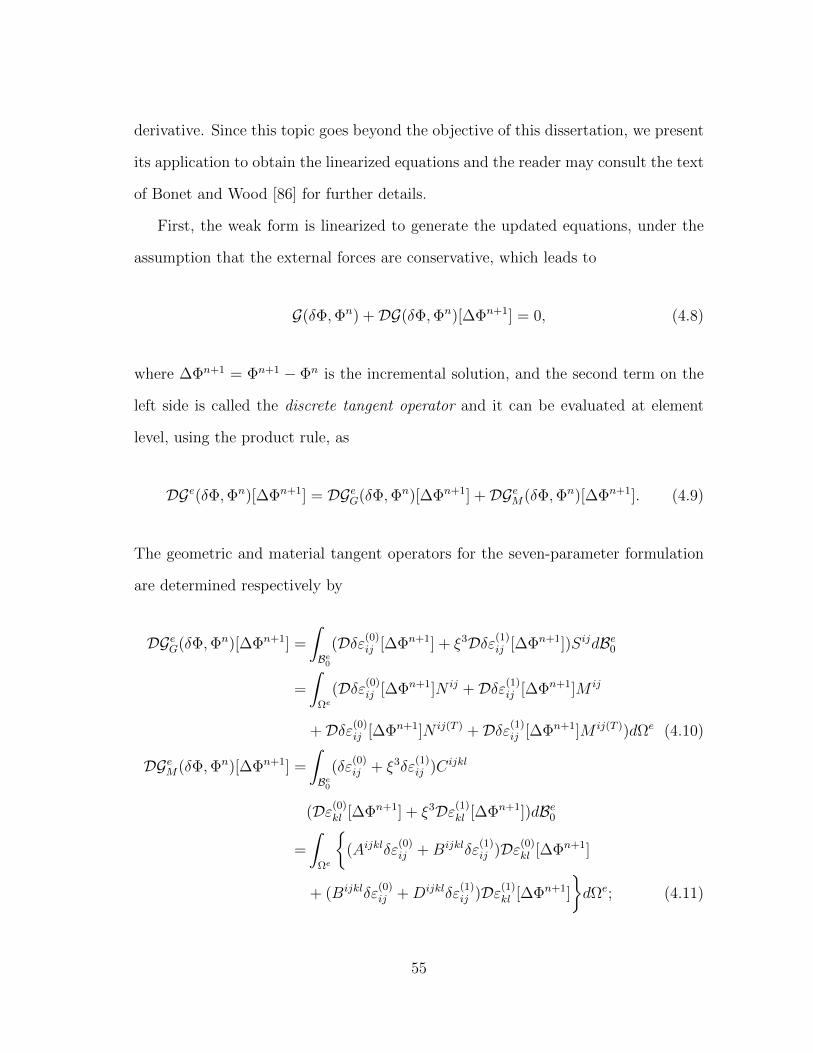
derivative. Since this topic goes beyond the objective of this dissertation, we present
its application to obtain the linearized equations and the reader may consult the text
of Bonet and Wood [86] for further details.
First, the weak form is linearized to generate the updated equations, under the
assumption that the external forces are conservative, which leads to
G(δΦ,Φn) +DG(δΦ,Φn)[∆Φn+1] = 0, (4.8)
where ∆Φn+1 = Φn+1 − Φn is the incremental solution, and the second term on the
left side is called the discrete tangent operator and it can be evaluated at element
level, using the product rule, as
DGe(δΦ,Φn)[∆Φn+1] = DGeG(δΦ,Φn)[∆Φn+1] +DGeM(δΦ,Φn)[∆Φn+1]. (4.9)
The geometric and material tangent operators for the seven-parameter formulation
are determined respectively by
DGeG(δΦ,Φn)[∆Φn+1] =
∫Be0
(Dδε(0)ij [∆Φn+1] + ξ3Dδε(1)
ij [∆Φn+1])SijdBe0
=
∫Ωe
(Dδε(0)ij [∆Φn+1]N ij +Dδε(1)
ij [∆Φn+1]M ij
+Dδε(0)ij [∆Φn+1]N ij(T ) +Dδε(1)
ij [∆Φn+1]M ij(T ))dΩe (4.10)
DGeM(δΦ,Φn)[∆Φn+1] =
∫Be0
(δε(0)ij + ξ3δε
(1)ij )Cijkl
(Dε(0)kl [∆Φn+1] + ξ3Dε(1)
kl [∆Φn+1])dBe0
=
∫Ωe
(Aijklδε
(0)ij +Bijklδε
(1)ij )Dε(0)
kl [∆Φn+1]
+ (Bijklδε(0)ij +Dijklδε
(1)ij )Dε(1)
kl [∆Φn+1]
dΩe; (4.11)
55

while for the twelve-parameter formulation are computed by
DGeG(δΦ,Φn)[∆Φn+1] =
∫Be0
(Dδε(0)ij [∆Φn+1] + ξ3Dδε(1)
ij [∆Φn+1]
+ (ξ3)2Dδε(2)ij [∆Φn+1])SijdBe0
=
∫Ωe
(Dδε(0)
ij [∆Φn+1]N ij +Dδε(1)ij [∆Φn+1]M ij (4.12)
+Dδε(2)ij [∆Φn+1]Oij +Dδε(0)
ij [∆Φn+1]N ij(T )
+Dδε(1)ij [∆Φn+1]M ij(T ) +Dδε(2)
ij [∆Φn+1]Oij(T ))dΩe
DGeM(δΦ,Φn)[∆Φn+1] =
∫Be0
(δε(0)ij + ξ3δε
(1)ij + (ξ3)2δε
(2)ij )Cijkl
(Dε(0)kl [∆Φn+1] + ξ3Dε(1)
kl [∆Φn+1] + (ξ3)2Dε(2)kl [∆Φn+1])dBe0
=
∫Ωe
(Aijklδε
(0)ij +Bijklδε
(1)ij +Dijklδε
(2)ij )Dε(0)
kl [∆Φn+1]
+ (Bijklδε(0)ij +Dijklδε
(1)ij + Eijklδε
(2)ij )Dε(1)
kl [∆Φn+1]
+ (Dijklδε(0)ij + Eijklδε
(1)ij +Gijklδε
(2)ij )Dε(2)
kl [∆Φn+1]
dΩe.
(4.13)
The contravariant component of the internal stress resultants N ij, M ij and Oij ap-
pearing in the discrete tangent operators may be evaluated as
N ij,M ij, Oij
=
∫ 1
−1
1, ξ3, (ξ3)2
Cijkl
[ε
(0)kl + ξ3ε
(1)kl + (ξ3)2ε
(2)kl
]Jdξ3, (4.14)
where the underlined term is only used for the 12-parameter formulation. The equiv-
alent terms, due to thermal load, are
N ij(T ),M ij(T ), Oij(T )
= −
∫ 1
−1
1, ξ3, (ξ3)2
α(ξ3)∆TCijklgklJdξ
3. (4.15)
56
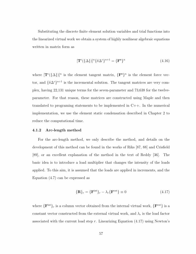
Substituting the discrete finite element solution variables and trial functions into
the linearized virtual work we obtain a system of highly nonlinear algebraic equations
written in matrix form as
[Te(∆)]nδ∆en+1 = Fen (4.16)
where [Te(∆)]n is the element tangent matrix, Fen is the element force vec-
tor, and δ∆en+1 is the incremental solution. The tangent matrices are very com-
plex, having 22,131 unique terms for the seven-parameter and 73,638 for the twelve-
parameter. For that reason, these matrices are constructed using Maple and then
translated to programing statements to be implemented in C++. In the numerical
implementation, we use the element static condensation described in Chapter 2 to
reduce the computational time.
4.1.2 Arc-length method
For the arc-length method, we only describe the method, and details on the
development of this method can be found in the works of Riks [87, 88] and Crisfield
[89], or an excellent explanation of the method in the text of Reddy [36]. The
basic idea is to introduce a load multiplier that changes the intensity of the loads
applied. To this aim, it is assumed that the loads are applied in increments, and the
Equation (4.7) can be expressed as
Rr = Fintr − λrFext ≡ 0 (4.17)
where Fintr is a column vector obtained from the internal virtual work, Fext is a
constant vector constructed from the external virtual work, and λr is the load factor
associated with the current load step r. Linearizing Equation (4.17) using Newton’s
57
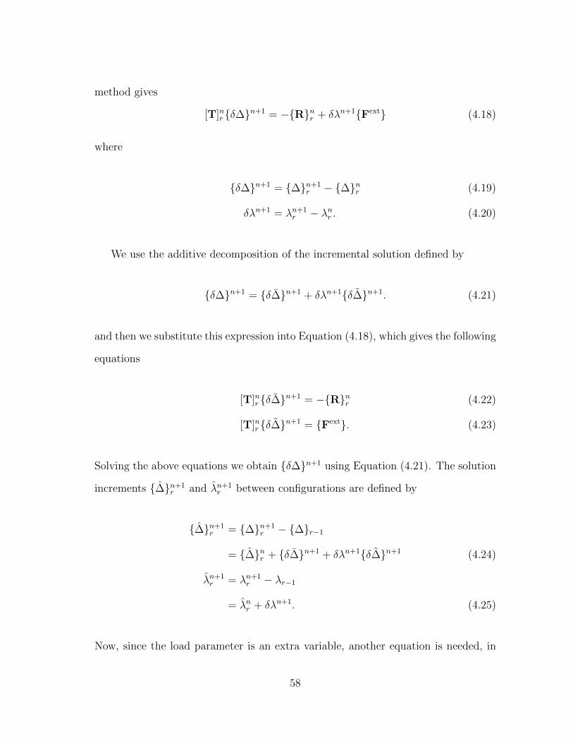
method gives
[T]nr δ∆n+1 = −Rnr + δλn+1Fext (4.18)
where
δ∆n+1 = ∆n+1r − ∆nr (4.19)
δλn+1 = λn+1r − λnr . (4.20)
We use the additive decomposition of the incremental solution defined by
δ∆n+1 = δ∆n+1 + δλn+1δ∆n+1. (4.21)
and then we substitute this expression into Equation (4.18), which gives the following
equations
[T]nr δ∆n+1 = −Rnr (4.22)
[T]nr δ∆n+1 = Fext. (4.23)
Solving the above equations we obtain δ∆n+1 using Equation (4.21). The solution
increments ∆n+1r and λn+1
r between configurations are defined by
∆n+1r = ∆n+1
r − ∆r−1
= ∆nr + δ∆n+1 + δλn+1δ∆n+1 (4.24)
λn+1r = λn+1
r − λr−1
= λnr + δλn+1. (4.25)
Now, since the load parameter is an extra variable, another equation is needed, in
58

order to solve the problem. For that reason, the cylindrical arc-length constrain
equation for δλn+1 is defined, and expressed by
κn+1r = ‖∆n+1
r ‖2 − (∆Lr)2 (4.26)
= b1(δλn+1)2 + b2δλn+1 + b3 = 0 (4.27)
where ∆Lr is the arc-length, ‖ · ‖ denotes the Euclidean norm, and the coefficients
b1, b2 and b3 are defined as
b1 = ‖δ∆n+1‖2
b2 = 2[(∆nr + δ∆n+1)Tδ∆n+1
]b3 = ‖∆nr + δ∆n+1‖2 − (∆Lr)
2. (4.28)
The solutions to the quadratic equations can be computed by
δλn+11,2 =
−b2 ±√b2
2 − 4b1b3
2b1
, (4.29)
and these produce two different configurations. We select the solution that is closer
to the previous displacement increment. To this aim, we choose the solution that has
a positive inner product of ∆n+1r with ∆nr . If both have positive inner products,
we select the one with ∆n+1r closest to ∆nr in the Euclidean metric. For the first
iteration of a given load step, we select ∆1r such that the inner product of ∆1
r
with the converged incremental solution from load step r − 1, ∆r−1, is positive
[90].
To initialize the solution we take λ0r−1 = 0, and δλ1 = 1. Then, Equation (4.23)
is solved for δ∆1. After that, we take δ∆1 = δλ1δ∆1 and we define the
59
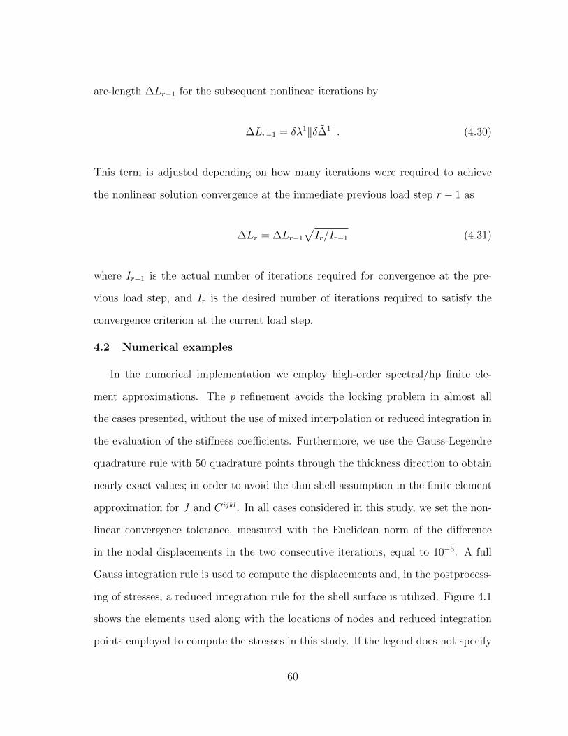
arc-length ∆Lr−1 for the subsequent nonlinear iterations by
∆Lr−1 = δλ1‖δ∆1‖. (4.30)
This term is adjusted depending on how many iterations were required to achieve
the nonlinear solution convergence at the immediate previous load step r − 1 as
∆Lr = ∆Lr−1
√Ir/Ir−1 (4.31)
where Ir−1 is the actual number of iterations required for convergence at the pre-
vious load step, and Ir is the desired number of iterations required to satisfy the
convergence criterion at the current load step.
4.2 Numerical examples
In the numerical implementation we employ high-order spectral/hp finite ele-
ment approximations. The p refinement avoids the locking problem in almost all
the cases presented, without the use of mixed interpolation or reduced integration in
the evaluation of the stiffness coefficients. Furthermore, we use the Gauss-Legendre
quadrature rule with 50 quadrature points through the thickness direction to obtain
nearly exact values; in order to avoid the thin shell assumption in the finite element
approximation for J and Cijkl. In all cases considered in this study, we set the non-
linear convergence tolerance, measured with the Euclidean norm of the difference
in the nodal displacements in the two consecutive iterations, equal to 10−6. A full
Gauss integration rule is used to compute the displacements and, in the postprocess-
ing of stresses, a reduced integration rule for the shell surface is utilized. Figure 4.1
shows the elements used along with the locations of nodes and reduced integration
points employed to compute the stresses in this study. If the legend does not specify
60
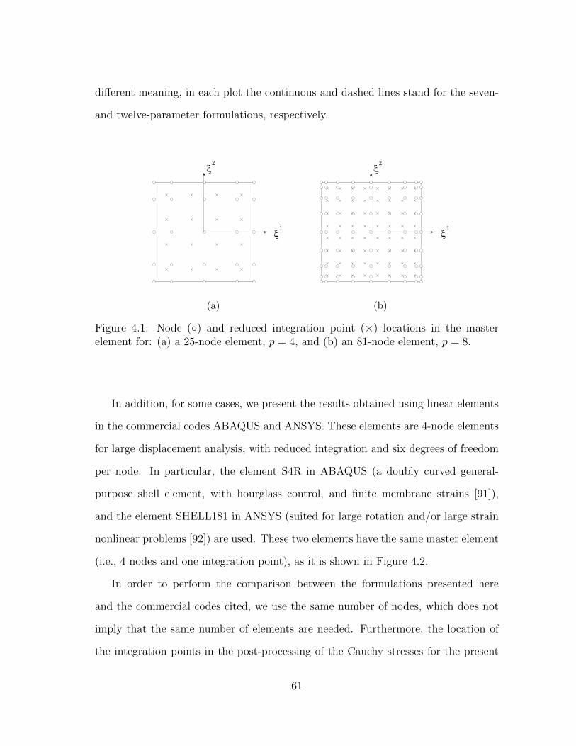
different meaning, in each plot the continuous and dashed lines stand for the seven-
and twelve-parameter formulations, respectively.
1
2
(a)
1
2
(b)
Figure 4.1: Node () and reduced integration point (×) locations in the masterelement for: (a) a 25-node element, p = 4, and (b) an 81-node element, p = 8.
In addition, for some cases, we present the results obtained using linear elements
in the commercial codes ABAQUS and ANSYS. These elements are 4-node elements
for large displacement analysis, with reduced integration and six degrees of freedom
per node. In particular, the element S4R in ABAQUS (a doubly curved general-
purpose shell element, with hourglass control, and finite membrane strains [91]),
and the element SHELL181 in ANSYS (suited for large rotation and/or large strain
nonlinear problems [92]) are used. These two elements have the same master element
(i.e., 4 nodes and one integration point), as it is shown in Figure 4.2.
In order to perform the comparison between the formulations presented here
and the commercial codes cited, we use the same number of nodes, which does not
imply that the same number of elements are needed. Furthermore, the location of
the integration points in the post-processing of the Cauchy stresses for the present
61
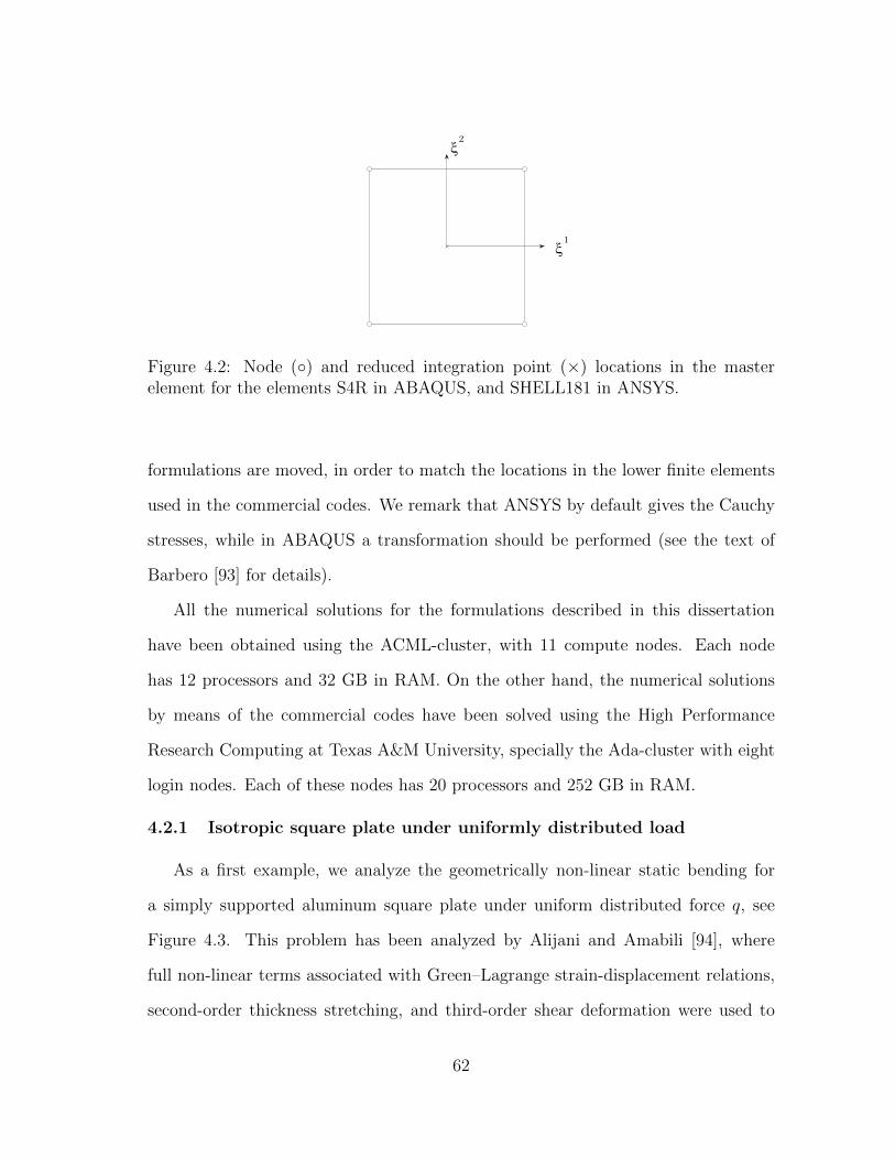
1
2
Figure 4.2: Node () and reduced integration point (×) locations in the masterelement for the elements S4R in ABAQUS, and SHELL181 in ANSYS.
formulations are moved, in order to match the locations in the lower finite elements
used in the commercial codes. We remark that ANSYS by default gives the Cauchy
stresses, while in ABAQUS a transformation should be performed (see the text of
Barbero [93] for details).
All the numerical solutions for the formulations described in this dissertation
have been obtained using the ACML-cluster, with 11 compute nodes. Each node
has 12 processors and 32 GB in RAM. On the other hand, the numerical solutions
by means of the commercial codes have been solved using the High Performance
Research Computing at Texas A&M University, specially the Ada-cluster with eight
login nodes. Each of these nodes has 20 processors and 252 GB in RAM.
4.2.1 Isotropic square plate under uniformly distributed load
As a first example, we analyze the geometrically non-linear static bending for
a simply supported aluminum square plate under uniform distributed force q, see
Figure 4.3. This problem has been analyzed by Alijani and Amabili [94], where
full non-linear terms associated with Green–Lagrange strain-displacement relations,
second-order thickness stretching, and third-order shear deformation were used to
62

describe the plate kinematics.
Figure 4.3: Simply supported aluminum square plate under uniform distributed load.
The geometrical parameters used are: L = 0.1 m, and h = 0.001 and 0.01 m; the
material properties are E = 70 GPa, ν = 0.3. Also, the non-dimensional pressure is
defined as P = qL4/(Eh4). We take advantage of the biaxial symmetry and model
only one quadrant of the domain, using a uniform mesh of 2 × 2, with p = 4. The
boundary conditions for the seven-parameter formulation are
at x = 0, L ux = uy = uz = ϕy = Ψ = 0
at y = 0, L ux = uy = uz = ϕx = Ψ = 0;
while for the twelve-parameter formulation are
at x = 0, L ux = uy = uz = ϕy = Ψy = Ψz = Θy = Θz = 0
at y = 0, L ux = uy = uz = ϕx = Ψx = Ψz = Θx = Θz = 0.
First, we study the response of a thin plate (h = 0.001 m) subjected to a uni-
formly distributed load q = 1.05 × 10⁸ Pa. Figures 4.4-4.6 show the maximum
transverse deflection uz(L/2, L/2)/h, the maximum transverse rotation ϕx(0, L/2),
63

and the thickness deformation for this thin plate, respectively. We can see that the
center deflection and the thickness deformation have very good agreement with the
ones reported in [94]. However, the maximum rotation obtained with the present
elements is overestimated when compared to the results given in [94]. Figure 4.7
presents the deformed configuration for this plate at the maximum load q.
0 3 6 9 12 150
2
4
6
8
10
12
14
16
P (×104)
uz(L/2,L/2
)/h
7-Parameter
12-Parameter
Alijani and Amabili [94]
Figure 4.4: Maximum deflection uz(L/2, L/2)/h for a thin aluminum square plate(h = 0.001 m).
For the thick plate (h = 0.01 m), the load applied is q = 1.05 × 10⁹ Pa. Fig-
ures 4.8-4.11 show the maximum transverse deflection uz(L/2, L/2)/h, the maximum
transverse rotation ϕx(0, L/2), the thickness deformation, and the variation of the
normal displacement across the thickness for this thick plate, respectively. We can
see from Figures 4.9-4.11, that the results obtained by means of the present formu-
lations have a very good agreement with the ones reported in [94]. However, the
maximum transverse deflection obtained with the present elements is smaller than
64

0 3 6 9 12 15−0.6
−0.5
−0.4
−0.3
−0.2
−0.1
0
P (×104)
ϕx(0,L/2
)
7-Parameter
12-Parameter
Alijani and Amabili [94]
Figure 4.5: Maximum rotation ϕx(0, L/2) for a thin aluminum square plate (h =0.001 m).
0 0.2 0.4 0.6 0.8 1−1
−0.8
−0.6
−0.4
−0.2
0·10−2
x/L
∆h/h
7-Parameter
12-Parameter
Alijani and Amabili [94]
Figure 4.6: Thickness deformation in a thin aluminum square plate (h = 0.001 m)when P = 1428.6.
65

Figure 4.7: Deformed configuration of an isotropic thin plate under uniform pressure,h = 0.001 m and q = 1.05× 10⁸ Pa.
the results given in [94].
0 30 60 90 120 1500
0.2
0.4
0.6
0.8
1
1.2
1.4
1.6
P
uz(L/2,L,2
)/h
7-Parameter
12-Parameter
Alijani and Amabili [94]
Figure 4.8: Maximum deflection uz(L/2, L/2)/h for a thick aluminum square plate(h = 0.01 m).
66

0 30 60 90 120 150−0.5
−0.4
−0.3
−0.2
−0.1
0
qL4/(Eh4)
ϕx(0,L/2
)
7-Parameter
12-Parameter
Alijani and Amabili [94]
Figure 4.9: Maximum rotation ϕx(0, L/2) for a thick aluminum square plate (h =0.01 m).
0 0.2 0.4 0.6 0.8 1
−0.06
−0.04
−0.02
0
x/L
∆h/h
7-Parameter
12-Parameter
Alijani and Amabili [94]
Figure 4.10: Thickness deformation in a thick aluminum square plate (h = 0.01 m)when P = 50.
67

−20 −15 −10 −5 0 5−1
−0.5
0
0.5
1
(u3 − uz)/h (×10−3)
ξ3
7-Parameter
12-Parameter
Alijani and Amabili [94]
Figure 4.11: Variation of the normal displacement across the thickness in a thickaluminum square plate (h = 0.01 m) at x/L = y/L = 0.5, when P = 50.
4.2.2 A simply supported isotropic cylindrical shell subjected to uni-
formly distributed radial forces
We analyze the example proposed by Amabili [26], a simply supported isotropic
cylindrical shell subjected to a non-displacement dependent pressure p (see Fig-
ure 4.12). The geometric parameters used are L = 0.52 m, R = 0.15 m, and h = 0.03
m, and the maximum load applied is q = 12 × 109 Pa. It is assumed that the shell
is made of stainless steel with properties E = 198 × 109 Pa and ν = 0.3. We ex-
ploited the symmetries and use one octant of the shell as our computational domain.
A uniform mesh of 4 × 4 with p = 8 is used. The boundary conditions for the
seven-parameter formulation are
at x = 0, L uy = uz = ϕy = ϕz = 0;
68
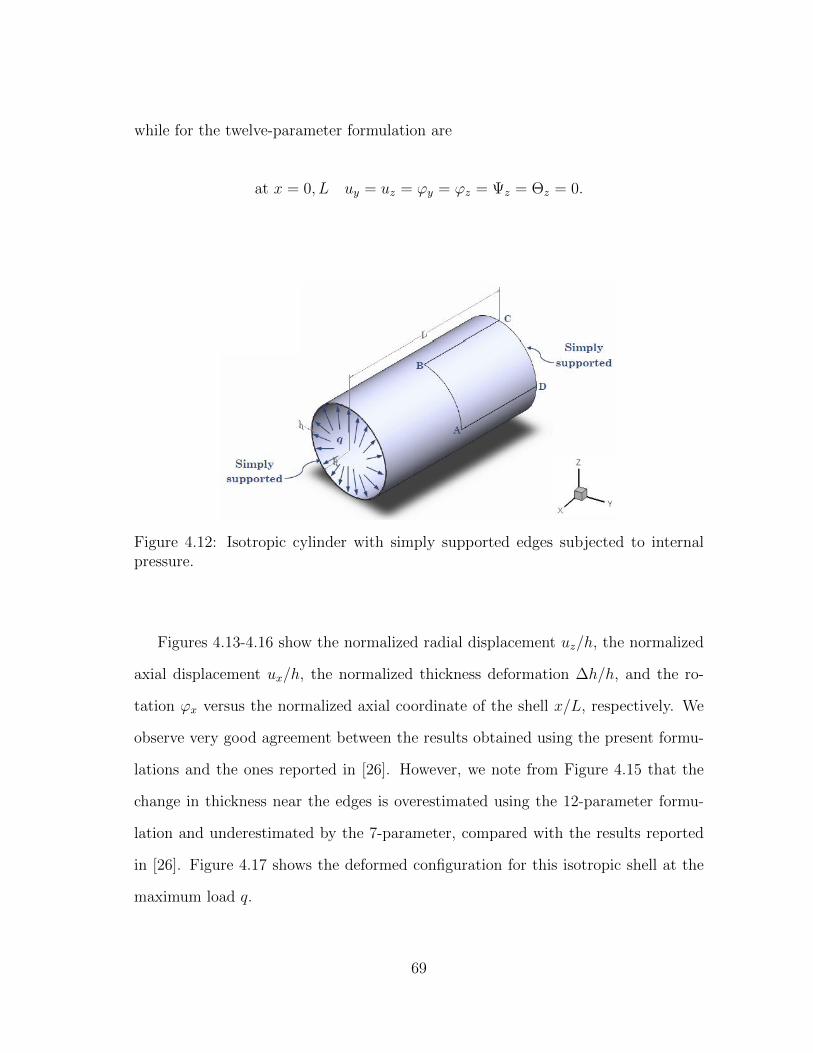
while for the twelve-parameter formulation are
at x = 0, L uy = uz = ϕy = ϕz = Ψz = Θz = 0.
Figure 4.12: Isotropic cylinder with simply supported edges subjected to internalpressure.
Figures 4.13-4.16 show the normalized radial displacement uz/h, the normalized
axial displacement ux/h, the normalized thickness deformation ∆h/h, and the ro-
tation ϕx versus the normalized axial coordinate of the shell x/L, respectively. We
observe very good agreement between the results obtained using the present formu-
lations and the ones reported in [26]. However, we note from Figure 4.15 that the
change in thickness near the edges is overestimated using the 12-parameter formu-
lation and underestimated by the 7-parameter, compared with the results reported
in [26]. Figure 4.17 shows the deformed configuration for this isotropic shell at the
maximum load q.
69

0 0.2 0.4 0.6 0.8 10
0.2
0.4
0.6
0.8
1
1.2
x/L
uz/h
7-Parameter
12-Parameter
Amabili [26]
Figure 4.13: Normalized radial displacement uz/h versus axial coordinate x/L.
0 0.2 0.4 0.6 0.8 1−1.2
−0.9
−0.6
−0.3
0
0.3
0.6
0.9
1.2
x/L
ux/h
7-Parameter
12-Parameter
Amabili [26]
Figure 4.14: Normalized axial displacement ux/h versus axial coordinate x/L.
70
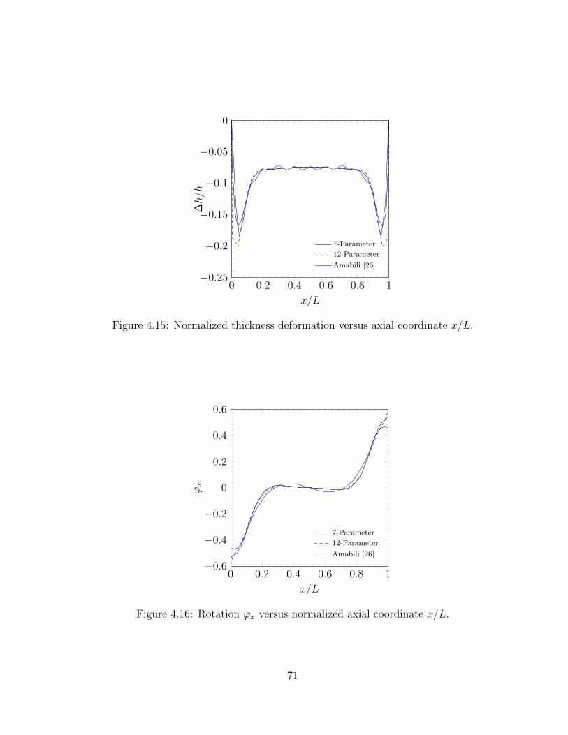
0 0.2 0.4 0.6 0.8 1−0.25
−0.2
−0.15
−0.1
−0.05
0
x/L
∆h/h
7-Parameter
12-Parameter
Amabili [26]
Figure 4.15: Normalized thickness deformation versus axial coordinate x/L.
0 0.2 0.4 0.6 0.8 1−0.6
−0.4
−0.2
0
0.2
0.4
0.6
x/L
ϕx
7-Parameter
12-Parameter
Amabili [26]
Figure 4.16: Rotation ϕx versus normalized axial coordinate x/L.
71

Figure 4.17: Deformed configuration of an isotropic cylinder under internal pressure,q = 198× 109 Pa.
4.2.3 Laminated composite plates under uniform pressure
We compare the experimental results obtained by Zaghloul[95], for the nonlin-
ear response of symmetrically laminated plates under uniform pressure q (see Fig-
ure 4.18), with the displacements predicted by means of the presented formulations.
The geometric parameters are: L = 12 in, and h = 0.138 in, while the maximum
pressure applied is q = 2 psi.
Figure 4.18: A simply supported plate under uniform distributed load of intensity q.
72
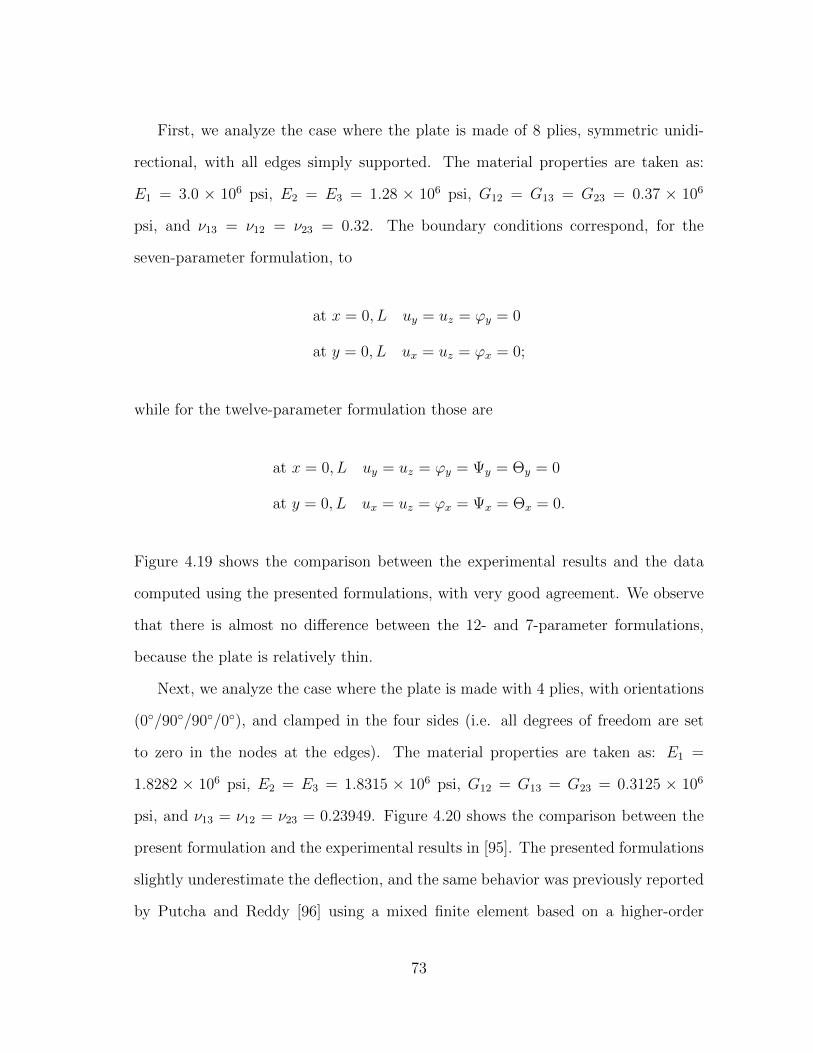
First, we analyze the case where the plate is made of 8 plies, symmetric unidi-
rectional, with all edges simply supported. The material properties are taken as:
E1 = 3.0 × 10⁶ psi, E2 = E3 = 1.28 × 10⁶ psi, G12 = G13 = G23 = 0.37 × 10⁶
psi, and ν13 = ν12 = ν23 = 0.32. The boundary conditions correspond, for the
seven-parameter formulation, to
at x = 0, L uy = uz = ϕy = 0
at y = 0, L ux = uz = ϕx = 0;
while for the twelve-parameter formulation those are
at x = 0, L uy = uz = ϕy = Ψy = Θy = 0
at y = 0, L ux = uz = ϕx = Ψx = Θx = 0.
Figure 4.19 shows the comparison between the experimental results and the data
computed using the presented formulations, with very good agreement. We observe
that there is almost no difference between the 12- and 7-parameter formulations,
because the plate is relatively thin.
Next, we analyze the case where the plate is made with 4 plies, with orientations
(0/90/90/0), and clamped in the four sides (i.e. all degrees of freedom are set
to zero in the nodes at the edges). The material properties are taken as: E1 =
1.8282 × 10⁶ psi, E2 = E3 = 1.8315 × 10⁶ psi, G12 = G13 = G23 = 0.3125 × 10⁶
psi, and ν13 = ν12 = ν23 = 0.23949. Figure 4.20 shows the comparison between the
present formulation and the experimental results in [95]. The presented formulations
slightly underestimate the deflection, and the same behavior was previously reported
by Putcha and Reddy [96] using a mixed finite element based on a higher-order
73
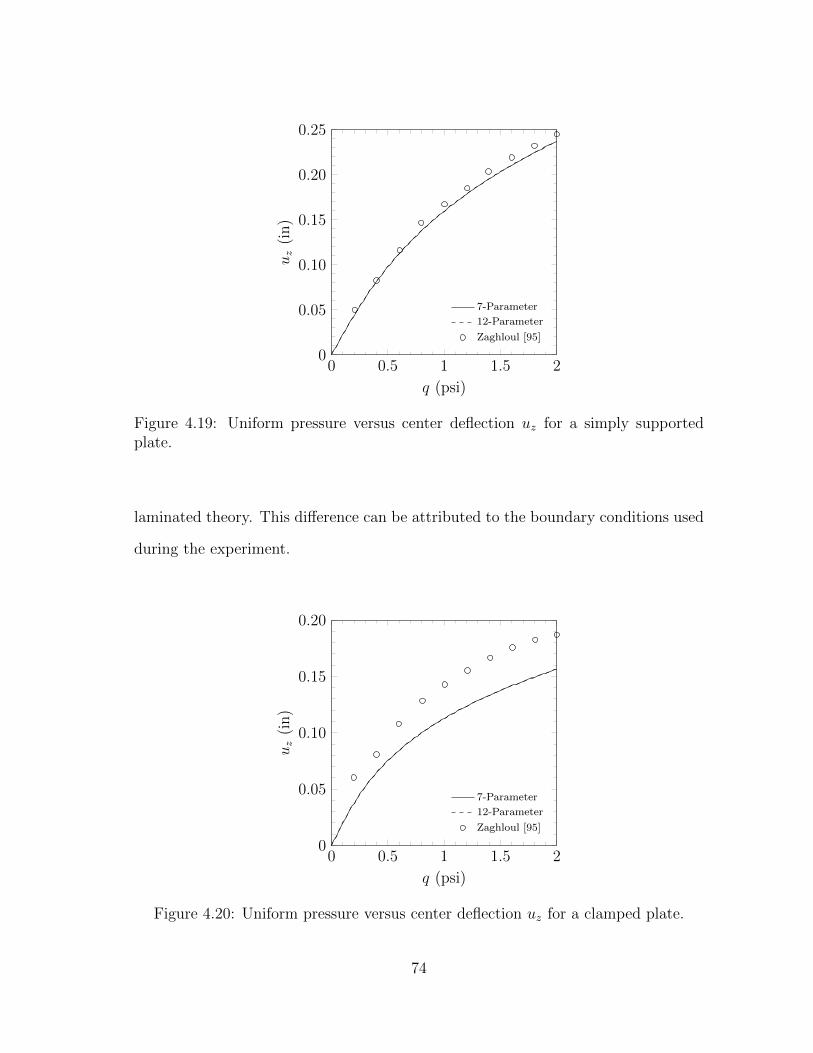
0 0.5 1 1.5 20
0.05
0.10
0.15
0.20
0.25
q (psi)
uz
(in)
7-Parameter
12-Parameter
Zaghloul [95]
Figure 4.19: Uniform pressure versus center deflection uz for a simply supportedplate.
laminated theory. This difference can be attributed to the boundary conditions used
during the experiment.
0 0.5 1 1.5 20
0.05
0.10
0.15
0.20
q (psi)
uz
(in)
7-Parameter
12-Parameter
Zaghloul [95]
Figure 4.20: Uniform pressure versus center deflection uz for a clamped plate.
74
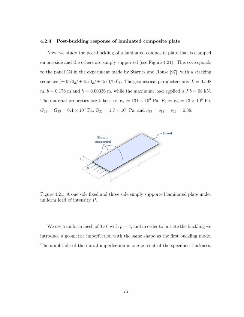
4.2.4 Post-buckling response of laminated composite plate
Now, we study the post-buckling of a laminated composite plate that is clamped
on one side and the others are simply supported (see Figure 4.21). This corresponds
to the panel C4 in the experiment made by Starnes and Rouse [97], with a stacking
sequence (±45/02/±45/02/±45/0/90)S. The geometrical parameters are: L = 0.508
m, b = 0.178 m and h = 0.00336 m, while the maximum load applied is Pb = 98 kN.
The material properties are taken as: E1 = 131 × 109 Pa, E2 = E3 = 13 × 109 Pa,
G12 = G13 = 6.4× 10⁹ Pa, G23 = 1.7× 10⁹ Pa, and ν13 = ν12 = ν23 = 0.38.
P
Fixed Simply
supported
Figure 4.21: A one side fixed and three side simply supported laminated plate underuniform load of intensity P .
We use a uniform mesh of 3×6 with p = 4, and in order to initiate the buckling we
introduce a geometric imperfection with the same shape as the first buckling mode.
The amplitude of the initial imperfection is one percent of the specimen thickness.
75
The boundary conditions for the seven-parameter formulation are
at x = 0 ux = uy = uz = ϕx = ϕy = ϕz = Ψ = 0
at x = L uz = ϕx = 0
at y = 0, b uz = 0;
while for the twelve-parameter formulation are
at x = 0 ux = uy = uz = ϕx = ϕy = ϕz = Ψx = Ψy = Ψz = Θx = Θy = Θz = 0
at x = L uz = ϕx = Ψx = Θx = 0
at y = 0, b uz = 0.
Figures 4.22 and 4.23 show the end shortening ux normalized by the analytical
end shortening ucr at buckling, and the out of plane deflection uz near a point
of maximum deflection normalized by the panel thickness h as a function of the
applied load P normalized by the analytical buckling load Pcr. We observe very
good agreement with the experimental results in [97], shown as symbols, and the
numerical results presented previously by Engelstad and Reddy [98]. Figure 4.24
shows the contour plot for the out of plane displacement uz at the maximum load.
4.2.5 Static analysis of a functionally grade plate
We reproduce the numerical results presented by Woo and Meguid [99], where the
analytical solution for the coupled large deflection of a simply supported functionally
graded square plate subjected to uniformly distributed load q is considered, see Figure
4.18. Displacements and the Cauchy stress distribution through the thickness at the
center of the plate obtained using the present formulations are compared with the
76

0 1 2 3 4 50
0.5
1
1.5
2
2.5
ux/ucr
P/P
cr
7-Parameter
12-Parameter
Starnes [97]
Figure 4.22: Normalized end shortening deflections versus nondimensionalized load.
0 1 2 30
0.5
1
1.5
2
2.5
uz/h
P/P
cr
7-Parameter
12-Parameter
Starnes [97]
Figure 4.23: Normalized out of plane deflection versus nondimensionalized load.
77

Figure 4.24: Deformed configuration of a laminated plate after buckling (contoursfor uz at Pb = 98 kN).
results presented in [99]. The geometrical parameters are: L = 0.2 m, and h = 0.01
m. The material properties used are summarized in Table 4.1, with aluminum for
the bottom surface (-) and alumina for the top surface (+). We take advantage of
the biaxial symmetry and model only one quadrant of the domain, using a uniform
mesh of 2× 2, with p = 4. The boundary conditions for the two formulations are
at x = 0, L uz = 0
at y = 0, L uz = 0.
Also, we use the following non-dimensional parameters: load parameterQ = qL4/(h4E−),
central deflection w = uz/h, and axial stress σ = σxxL2/(h2E−).
4.2.5.1 FGM plate under mechanical load
First, we study the mechanical response of the plate under a uniformly distributed
load q = 1.75 × 10⁸ Pa. Figure 4.25 presents the dimensionless load parameter, Q,
78
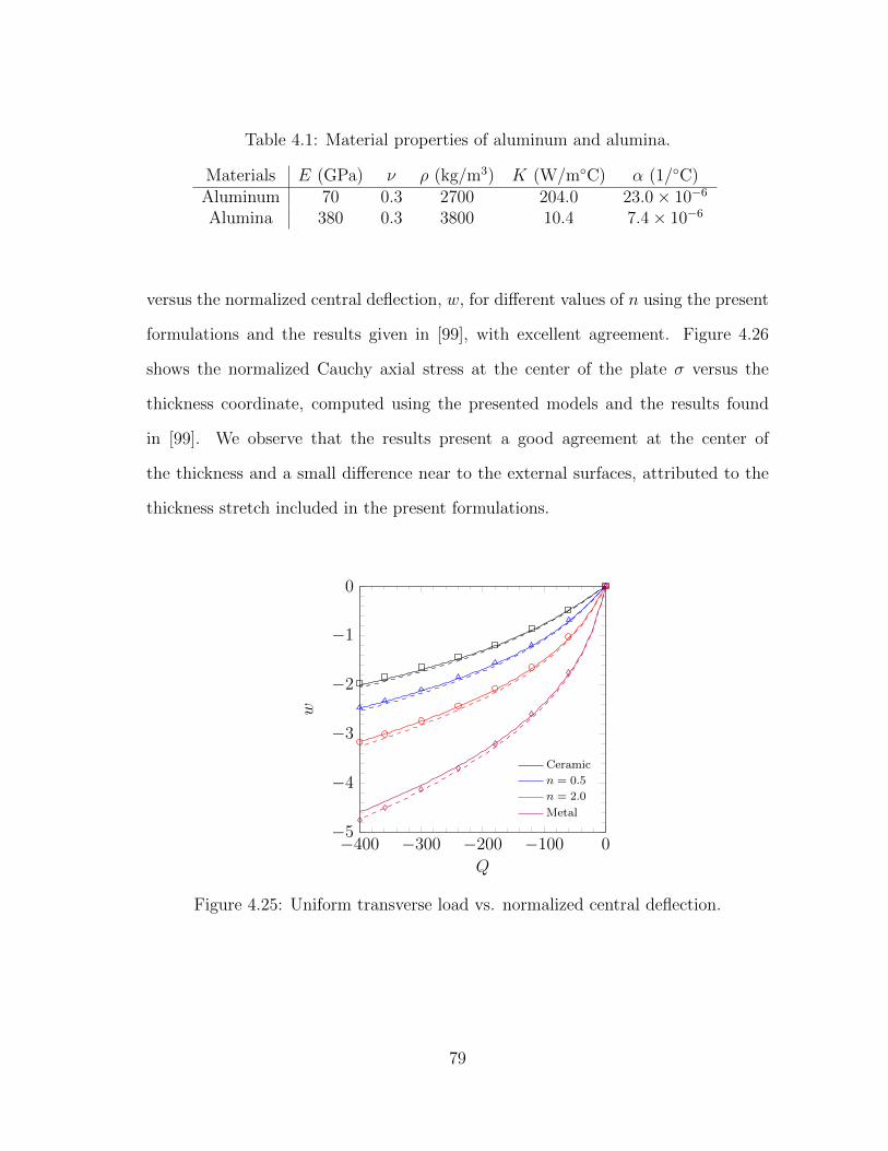
Table 4.1: Material properties of aluminum and alumina.
Materials E (GPa) ν ρ (kg/m3) K (W/mC) α (1/C)Aluminum 70 0.3 2700 204.0 23.0× 10⁻⁶
Alumina 380 0.3 3800 10.4 7.4× 10⁻⁶
versus the normalized central deflection, w, for different values of n using the present
formulations and the results given in [99], with excellent agreement. Figure 4.26
shows the normalized Cauchy axial stress at the center of the plate σ versus the
thickness coordinate, computed using the presented models and the results found
in [99]. We observe that the results present a good agreement at the center of
the thickness and a small difference near to the external surfaces, attributed to the
thickness stretch included in the present formulations.
−400 −300 −200 −100 0−5
−4
−3
−2
−1
0
Q
w
Ceramic
n = 0.5
n = 2.0
Metal
Figure 4.25: Uniform transverse load vs. normalized central deflection.
79

−1 −0.5 0 0.5 1−40
−20
0
20
40
60
80
ξ3
σ
Ceramic
n = 0.5
n = 2.0
Metal
Figure 4.26: Dimensionless axial stress along the thickness, at the center of the platesunder the dimensionless load Q = −400.
4.2.5.2 FGM plate under mechanical and thermal loads
The same plate considered in the previous example, in addition to the uniform
load, is also subjected to a one dimensional temperature field. The lower surface is
held at 20C and a heat flux of 9.152× 10⁵ W/m2 is applied from the upper surface
to the lower. The initial stress free state is assumed to exist at a temperature of
T0 = 0C. In this case, the maximum load applied is q = 3.5× 10⁷ Pa.
Figure 4.27 shows the temperature distribution through the thickness of func-
tionally graded plates for different values of n. From this plot, we can see that the
temperatures for the ceramic, n = 0.5, n = 2, and metal correspond to 900.00, 221.97,
119.86, and 64.86C, respectively. Figure 4.28 presents the dimensionless load pa-
rameter, Q, versus the normalized central deflection, w, with excellent agreement
and slightly higher deflections for the 12-Parameter formulation.
Figure 4.29 presents the normalized Cauchy axial stress at the center of the plate
80

−1 −0.5 0 0.5 10
100
200
300
400
500
600
700
800
900
ξ3
Tem
per
ature
dis
trib
uti
on
Ceramic
n = 0.5
n = 2.0
Metal
Figure 4.27: Temperature field through the thickness of the FG plates.
−80 −60 −40 −20 0−2.5
−2
−1.5
−1
−0.5
0
0.5
Q
w
Ceramic
n = 0.5
n = 2.0
Metal
Figure 4.28: Uniform transverse load vs. normalized central deflection of FG platesunder mechanical and thermal loads.
σ versus the thickness coordinate ξ3, for the presented models and the results found
in [99]. The results show good agreement for the metal, and the results look shifted
81

as the value of n decreases. From Figure 4.27, we observe that this behavior is related
to the temperature difference between the top and bottom surfaces ∆T , and the use
of three dimensional constitutive equations in the present models, against the results
based on the classical plate theory presented in [99].
−1 −0.5 0 0.5 1−40
−30
−20
−10
0
10
20
30
ξ3
σ
Ceramic
n = 0.5
n = 2.0
Metal
Figure 4.29: Dimensionless axial stress along the thickness, at the center of the platesunder the dimensionless load Q = −80 and thermal load.
In order to check the correctness of the present formulations, we compare the
maximum displacements, and the stresses at the top and bottom surfaces for the
ceramic case (the one with greater difference in the stress values), using the formula-
tions developed, solid elements in the commercial codes ANSYS (element SOLID186)
and ABAQUS (element C3D8RT), and the analytical solution found in reference [99].
For the commercial codes, we also apply symmetry and model the domain using a
uniform mesh of 24×24×10, with linear elements. Table 4.2 shows this comparison.
The analytical solution has lower displacement and stress at the bottom surface,
82
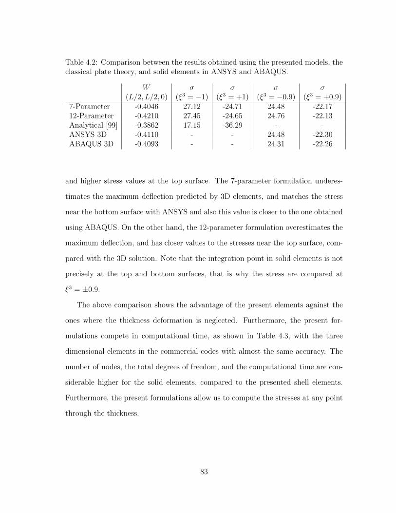
Table 4.2: Comparison between the results obtained using the presented models, theclassical plate theory, and solid elements in ANSYS and ABAQUS.
W(L/2, L/2, 0)
σ(ξ3 = −1)
σ(ξ3 = +1)
σ(ξ3 = −0.9)
σ(ξ3 = +0.9)
7-Parameter -0.4046 27.12 -24.71 24.48 -22.1712-Parameter -0.4210 27.45 -24.65 24.76 -22.13Analytical [99] -0.3862 17.15 -36.29 - -ANSYS 3D -0.4110 - - 24.48 -22.30ABAQUS 3D -0.4093 - - 24.31 -22.26
and higher stress values at the top surface. The 7-parameter formulation underes-
timates the maximum deflection predicted by 3D elements, and matches the stress
near the bottom surface with ANSYS and also this value is closer to the one obtained
using ABAQUS. On the other hand, the 12-parameter formulation overestimates the
maximum deflection, and has closer values to the stresses near the top surface, com-
pared with the 3D solution. Note that the integration point in solid elements is not
precisely at the top and bottom surfaces, that is why the stress are compared at
ξ3 = ±0.9.
The above comparison shows the advantage of the present elements against the
ones where the thickness deformation is neglected. Furthermore, the present for-
mulations compete in computational time, as shown in Table 4.3, with the three
dimensional elements in the commercial codes with almost the same accuracy. The
number of nodes, the total degrees of freedom, and the computational time are con-
siderable higher for the solid elements, compared to the presented shell elements.
Furthermore, the present formulations allow us to compute the stresses at any point
through the thickness.
83

Table 4.3: Number of nodes, total degrees of freedom (DOF), and computationaltime used (for the presented models, and solid elements in ANSYS and ABAQUS)to solve a ceramic plate under thermo-mechanical loads.
Elements Nodes Total DOF Time (s)7-Parameter 4 81 567 912-Parameter 4 81 972 18ANSYS 3D 5,760 6,875 20,625 107ABAQUS 3D 5,760 6,875 20,625 66
4.2.6 A cantilevered isotropic plate strip under an end shear force
We consider an isotropic cantilevered plate subjected to a distributed end shear
force on the free end, as shown in Figure 4.30. This problem has been previously
explored by Horrigmoe [100], Simo et al. [101], Park [102], Betsch [103], El-Abbasi
and Meguid [104], and Sze el al. [105], among others. We use the data presented in
the latest paper, which correspond to: L = 10.0, b = 1.0, h = 0.1, and q = 5.0. Also,
the same material properties used in [105] are taken: E = 1.2 × 10⁶, and ν = 0.0.
The boundary conditions for the seven-parameter formulation are
at x = 0 ux = uy = uz = ϕx = ϕy = ϕz = Ψ = 0
while for the twelve-parameter formulation are
at x = 0 ux = uy = uz = ϕx = ϕy = ϕz = Ψx = Ψy = Ψz = Θx = Θy = Θz = 0.
Figures 4.31 and 4.32 contain plots of the end shear force versus the tip transverse
displacement of the cantilever plate strip. We utilized a uniform mesh of 1 × 4
spectral elements with polynomial degree of p = 4 (i.e., a 25-node element with a
static condensation of the internal nodal degrees of freedom), while for ABAQUS
84

Figure 4.30: Cantilever plate strip under an end shear force.
and ANSYS we used a uniform mesh of 4×16 4-node respective elements. Deformed
configurations of the plate strip for various load values are shown in Figure 4.33.
The displacements obtained from all four show very good agreement with the ones
obtained in [105] and, more recently, in [23] and [24].
0 1 2 3 4 5−4
−3
−2
−1
0
q
Tip
defl
ecti
ons
7 Parameter
12 Parameter
ABAQUS
ANSYS
Figure 4.31: End shear force q vs. tip-deflection ux, for an isotropic cantileveredplate strip (ν = 0.0).
85

0 1 2 3 4 50
2
4
6
8
q
Tip
defl
ecti
ons
7 Parameter
12 Parameter
ABAQUS
ANSYS
Figure 4.32: End shear force q vs. tip-deflection uz, for an isotropic cantileveredplate strip (ν = 0.0).
Figure 4.33: Deformed configurations of an isotropic cantilever plate strip subjectedto an end shear force (load values q = 0.0, 1.0, ..., 5.0).
The maximum values of σxx and σzz are shown in Figures 4.34 and 4.35. The
stress σxx is evaluated at point A: 0.3125, 0.375,−h/2 and stress σzz is evaluated at
86
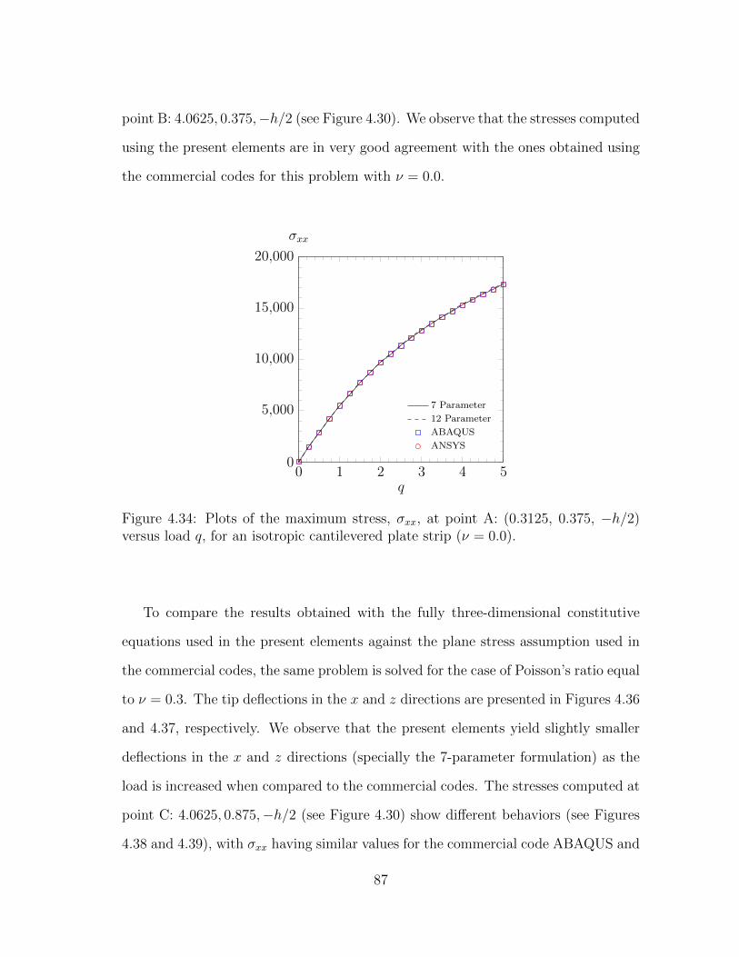
point B: 4.0625, 0.375,−h/2 (see Figure 4.30). We observe that the stresses computed
using the present elements are in very good agreement with the ones obtained using
the commercial codes for this problem with ν = 0.0.
0 1 2 3 4 50
5,000
10,000
15,000
20,000
q
σxx
7 Parameter
12 Parameter
ABAQUS
ANSYS
Figure 4.34: Plots of the maximum stress, σxx, at point A: (0.3125, 0.375, −h/2)versus load q, for an isotropic cantilevered plate strip (ν = 0.0).
To compare the results obtained with the fully three-dimensional constitutive
equations used in the present elements against the plane stress assumption used in
the commercial codes, the same problem is solved for the case of Poisson’s ratio equal
to ν = 0.3. The tip deflections in the x and z directions are presented in Figures 4.36
and 4.37, respectively. We observe that the present elements yield slightly smaller
deflections in the x and z directions (specially the 7-parameter formulation) as the
load is increased when compared to the commercial codes. The stresses computed at
point C: 4.0625, 0.875,−h/2 (see Figure 4.30) show different behaviors (see Figures
4.38 and 4.39), with σxx having similar values for the commercial code ABAQUS and
87
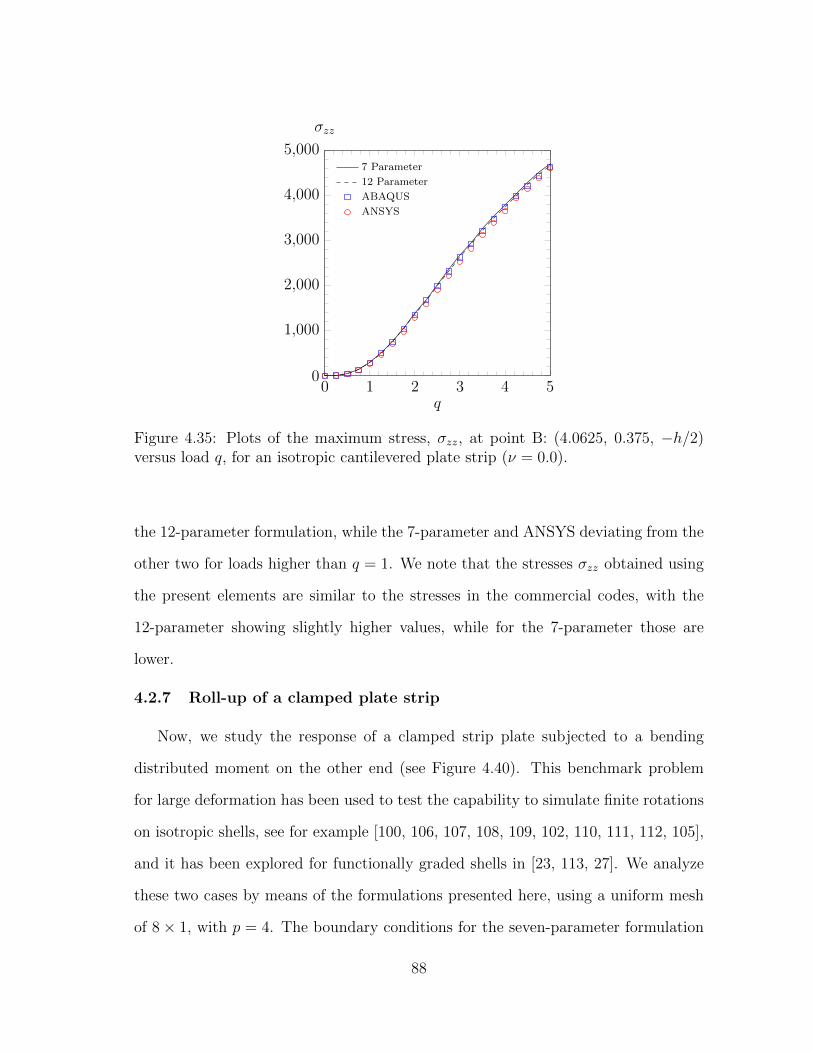
0 1 2 3 4 50
1,000
2,000
3,000
4,000
5,000
q
σzz
7 Parameter
12 Parameter
ABAQUS
ANSYS
Figure 4.35: Plots of the maximum stress, σzz, at point B: (4.0625, 0.375, −h/2)versus load q, for an isotropic cantilevered plate strip (ν = 0.0).
the 12-parameter formulation, while the 7-parameter and ANSYS deviating from the
other two for loads higher than q = 1. We note that the stresses σzz obtained using
the present elements are similar to the stresses in the commercial codes, with the
12-parameter showing slightly higher values, while for the 7-parameter those are
lower.
4.2.7 Roll-up of a clamped plate strip
Now, we study the response of a clamped strip plate subjected to a bending
distributed moment on the other end (see Figure 4.40). This benchmark problem
for large deformation has been used to test the capability to simulate finite rotations
on isotropic shells, see for example [100, 106, 107, 108, 109, 102, 110, 111, 112, 105],
and it has been explored for functionally graded shells in [23, 113, 27]. We analyze
these two cases by means of the formulations presented here, using a uniform mesh
of 8× 1, with p = 4. The boundary conditions for the seven-parameter formulation
88

0 1 2 3 4 5−4
−3
−2
−1
0
q
Tip
defl
ecti
ons
7 Parameter
12 Parameter
ABAQUS
ANSYS
Figure 4.36: End shear force q vs. tip-deflection ux, for an isotropic cantileveredplate strip (ν = 0.3).
0 1 2 3 4 50
2
4
6
8
q
Tip
defl
ecti
ons
7 Parameter
12 Parameter
ABAQUS
ANSYS
Figure 4.37: End shear force vs. tip-deflection uz, for an isotropic cantilevered platestrip (ν = 0.3).
are
at x = 0 ux = uy = uz = ϕx = ϕy = ϕz = Ψ = 0
89

0 1 2 3 4 50
2,000
4,000
6,000
q
σxx
7 Parameter
12 Parameter
ABAQUS
ANSYS
Figure 4.38: Plots of the stress, σxx, at point C: (4.0625, 0.875, −h/2) versus load q,for an isotropic cantilevered plate strip (ν = 0.3).
0 1 2 3 4 50
1,000
2,000
3,000
4,000
5,000
q
σzz
7 Parameter
12 Parameter
ABAQUS
ANSYS
Figure 4.39: Plots of the maximum stress, σzz, at point C: (4.0625, 0.875, −h/2)versus load q, for an isotropic cantilevered plate strip (ν = 0.3).
90
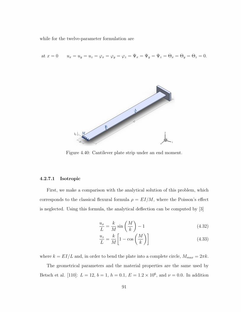
while for the twelve-parameter formulation are
at x = 0 ux = uy = uz = ϕx = ϕy = ϕz = Ψx = Ψy = Ψz = Θx = Θy = Θz = 0.
Figure 4.40: Cantilever plate strip under an end moment.
4.2.7.1 Isotropic
First, we make a comparison with the analytical solution of this problem, which
corresponds to the classical flexural formula ρ = EI/M , where the Poisson’s effect
is neglected. Using this formula, the analytical deflection can be computed by [3]
uxL
=k
Msin
(M
k
)− 1 (4.32)
uzL
=k
M
[1− cos
(M
k
)](4.33)
where k = EI/L and, in order to bend the plate into a complete circle, Mmax = 2πk.
The geometrical parameters and the material properties are the same used by
Betsch et al. [110]: L = 12, b = 1, h = 0.1, E = 1.2× 10⁶, and ν = 0.0. In addition
91

to the analytical solution, this problem is also analyzed using the commercial codes
ANSYS and ABAQUS with a uniform mesh of 32 × 4. Figures 4.41 and 4.42 show
the tip deflections in the x and z directions, respectively, with excellent agreement
for all the cases presented. Figure 4.43 shows deformed configurations for various
loads.
0 0.2 0.4 0.6 0.8 1
−15
−10
−5
0
M/Mmax
Tip
defl
ecti
ons
7 Parameter
12 Parameter
ABAQUS
ANSYS
Analytical
Figure 4.41: End moment vs. tip-deflection ux, for an isotropic cantilevered platestrip.
Figures 4.44 and 4.45 present the maximum stresses in the x and z directions,
respectively. We observe good agreement for the stress σxx, except for the values
computed using ANSYS which overestimate the values of the presented formulations
and ABAQUS. Also, there is a small difference in the stresses in the z direction
between the four codes used in the intermediate region, and these values become
closer at the maximum load.
92
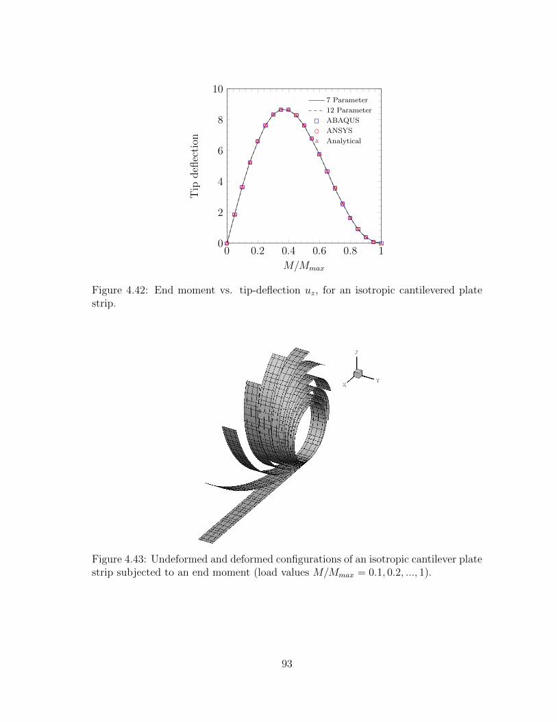
0 0.2 0.4 0.6 0.8 10
2
4
6
8
10
M/Mmax
Tip
defl
ecti
on
7 Parameter
12 Parameter
ABAQUS
ANSYS
Analytical
Figure 4.42: End moment vs. tip-deflection uz, for an isotropic cantilevered platestrip.
Figure 4.43: Undeformed and deformed configurations of an isotropic cantilever platestrip subjected to an end moment (load values M/Mmax = 0.1, 0.2, ..., 1).
93
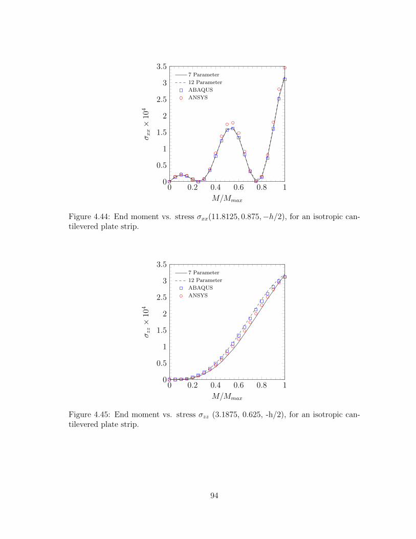
0 0.2 0.4 0.6 0.8 10
0.5
1
1.5
2
2.5
3
3.5
M/Mmax
σxx×
104
7 Parameter
12 Parameter
ABAQUS
ANSYS
Figure 4.44: End moment vs. stress σxx(11.8125, 0.875,−h/2), for an isotropic can-tilevered plate strip.
0 0.2 0.4 0.6 0.8 10
0.5
1
1.5
2
2.5
3
3.5
M/Mmax
σzz×
104
7 Parameter
12 Parameter
ABAQUS
ANSYS
Figure 4.45: End moment vs. stress σzz (3.1875, 0.625, -h/2), for an isotropic can-tilevered plate strip.
94

4.2.7.2 Functionally graded
In this case, we scale the geometry of the plate and now it is defined by the
parameters L = 0.12 m, b = 0.01 m, and h = 0.001 m; and the maximum moment
applied is Mmax = 7.05 N-m. The material properties are taken as: E− = 70 × 109
Pa, E+ = 151 × 109 Pa, and ν = 0.3, which correspond to aluminum and zirconia,
respectively [82].
Figures 4.46 and 4.47 contain plots of the end moment versus the tip transverse
displacement of the cantilever plate for various values of the power-law index n, for
the 7- and 12-parameter formulations. In all the cases, the displacements are plotted
until the plate folds into one complete loop, even though additional loops can be
achieved. The results show similar behavior to the ones obtained in [22], where
the authors were not able to obtain one complete loop for inhomogeneous shells.
We observe better behavior for 12-parameter formulation for finite rotations, giving
more smooth curves in the vertical displacement uz, after the plate reaches its higher
tip displacement.
The maximum stresses σxx and σzz for isotropic as well as for functionally graded
cantilever plate strips under applied bending moment are shown in Figures 4.48 and
4.49. The stress σxx is evaluated at point A: 25L/64, 7b/8, −h/2 and stress σzz
is evaluated at point B: 49L/64, 7b/8, −h/2 (see Figure 4.40). The stresses show
a similar behavior to the response for the metal structure, since they are located
at the bottom surface. Also, the stresses obtained by means of the 12-parameter
formulation present different intermediate behavior, compared with the 7-parameter
formulation.
95
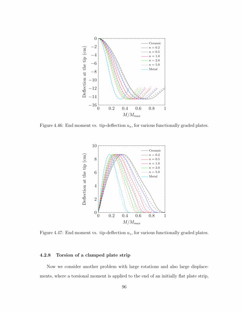
0 0.2 0.4 0.6 0.8 1−16
−14
−12
−10
−8
−6
−4
−2
0
M/Mmax
Defl
ecti
onat
the
tip
(cm
)
Ceramic
n = 0.2
n = 0.5
n = 1.0
n = 2.0
n = 5.0
Metal
Figure 4.46: End moment vs. tip-deflection ux, for various functionally graded plates.
0 0.2 0.4 0.6 0.8 10
2
4
6
8
10
M/Mmax
Defl
ecti
onat
the
tip
(cm
)
Ceramic
n = 0.2
n = 0.5
n = 1.0
n = 2.0
n = 5.0
Metal
Figure 4.47: End moment vs. tip-deflection uz, for various functionally graded plates.
4.2.8 Torsion of a clamped plate strip
Now we consider another problem with large rotations and also large displace-
ments, where a torsional moment is applied to the end of an initially flat plate strip,
96
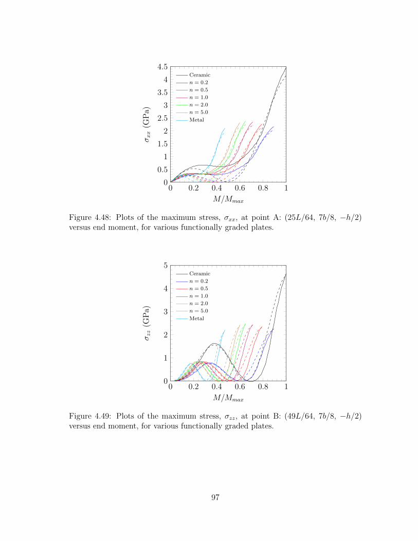
0 0.2 0.4 0.6 0.8 10
0.5
1
1.5
2
2.5
3
3.5
4
4.5
M/Mmax
σxx
(GP
a)
Ceramic
n = 0.2
n = 0.5
n = 1.0
n = 2.0
n = 5.0
Metal
Figure 4.48: Plots of the maximum stress, σxx, at point A: (25L/64, 7b/8, −h/2)versus end moment, for various functionally graded plates.
0 0.2 0.4 0.6 0.8 10
1
2
3
4
5
M/Mmax
σzz
(GP
a)
Ceramic
n = 0.2
n = 0.5
n = 1.0
n = 2.0
n = 5.0
Metal
Figure 4.49: Plots of the maximum stress, σzz, at point B: (49L/64, 7b/8, −h/2)versus end moment, for various functionally graded plates.
97

as shown in Figure 4.50. This example has been previously analyzed by Simo et al.
[107], Parisch [114], Park et al. [102] and Arciniega [3]; where rotations up to 180 for
the first three, and 270 degrees for the last one could be achieved. The geometrical
parameters are: L = 10, b = 1, and h = 0.1. This model is analyzed using an
isotropic material with properties: E = 12.0 × 10⁶, and ν = 0.3, the same used in
[3]. The boundary conditions applied for the seven-parameter formulation are
at x = 0 ux = uy = uz = ϕx = ϕy = ϕz = Ψ = 0;
while for the twelve-parameter formulation are
at x = 0 ux = uy = uz = ϕx = ϕy = ϕz = Ψx = Ψy = Ψz = Θx = Θy = Θz = 0.
A
B
T
Figure 4.50: Cantilever plate strip under an end torsional moment.
For the presented formulations, we use a uniform mesh of 8×1, with p = 4, while
for the commercial codes a uniform mesh of 32×4, with linear elements, is used. The
98

tip deflection in the z direction, uz, versus the applied torsional moment (T = 1000)
for points A and B are presented in the Figures 4.51 and 4.52, respectively. The
maximum load could only be applied to the 7-parameter formulation. ANSYS is
only able to reproduce this behavior until T = 100, even with very small load steps
(1/100000). On the other hand, for ABAQUS and the 12-parameter formulation, the
maximum torsion moments are T = 650 and 820, respectively. Figure 4.53 shows
the deformed configurations at the maximum load that could be achieved using
the presented formulations. We remark that, for the 12-parameter formulation, the
refinement in the mesh or the increasing in the p-level does not alleviate the locking,
and lower rotations are obtained. This behavior is attributed to the volumetric-
locking. However, since this is the only case where the total load cannot be achieved,
further studies are needed before arriving at any conclusion.
0 200 400 600 800 1,000−0.6
−0.4
−0.2
0
0.2
0.4
0.6
T
Tip
defl
ecti
ons
7 Parameter
12 Parameter
ABAQUS
ANSYS
Figure 4.51: End torsion moment versus tip-deflection uz at point A.
For completeness, we examine the behavior of the stress σxx near to the base.
99

0 200 400 600 800 1,000−0.6
−0.4
−0.2
0
0.2
0.4
0.6
T
Tip
defl
ecti
ons
7 Parameter
12 Parameter
ABAQUS
ANSYS
Figure 4.52: End torsion moment versus tip-deflection uz at point B.
(a) (b)
Figure 4.53: Deformed configuration at the maximum load achieved for the: (a) 7-(T = 1000) and (b) 12-parameter (T = 820) formulations.
Figure 4.54 shows this stress, up to the maximum loads achieved. We observe good
agreement between the stresses computed using the 7- and 12-parameter formula-
tions. The stresses in ABAQUS, as happened with the displacements, differ from
the present formulations after the plate rotates 90.
100
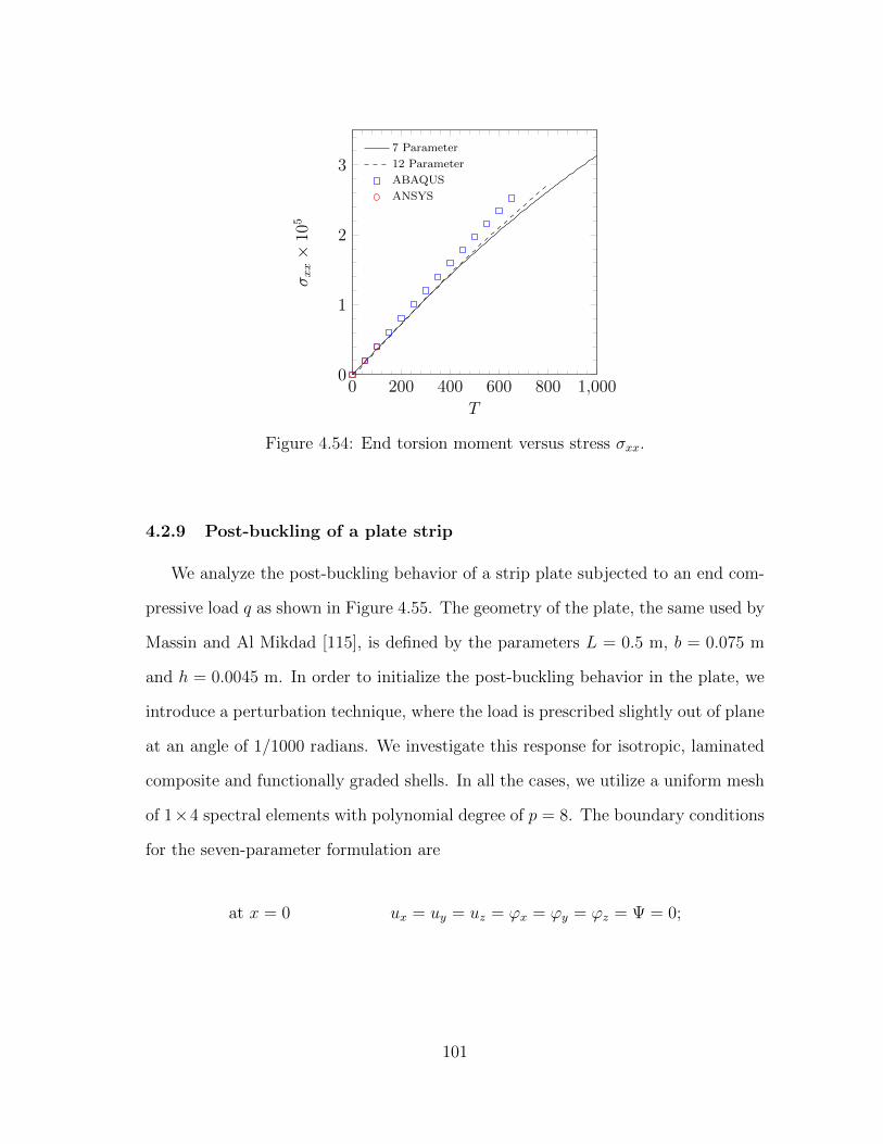
0 200 400 600 800 1,0000
1
2
3
T
σxx×
105
7 Parameter
12 Parameter
ABAQUS
ANSYS
Figure 4.54: End torsion moment versus stress σxx.
4.2.9 Post-buckling of a plate strip
We analyze the post-buckling behavior of a strip plate subjected to an end com-
pressive load q as shown in Figure 4.55. The geometry of the plate, the same used by
Massin and Al Mikdad [115], is defined by the parameters L = 0.5 m, b = 0.075 m
and h = 0.0045 m. In order to initialize the post-buckling behavior in the plate, we
introduce a perturbation technique, where the load is prescribed slightly out of plane
at an angle of 1/1000 radians. We investigate this response for isotropic, laminated
composite and functionally graded shells. In all the cases, we utilize a uniform mesh
of 1×4 spectral elements with polynomial degree of p = 8. The boundary conditions
for the seven-parameter formulation are
at x = 0 ux = uy = uz = ϕx = ϕy = ϕz = Ψ = 0;
101
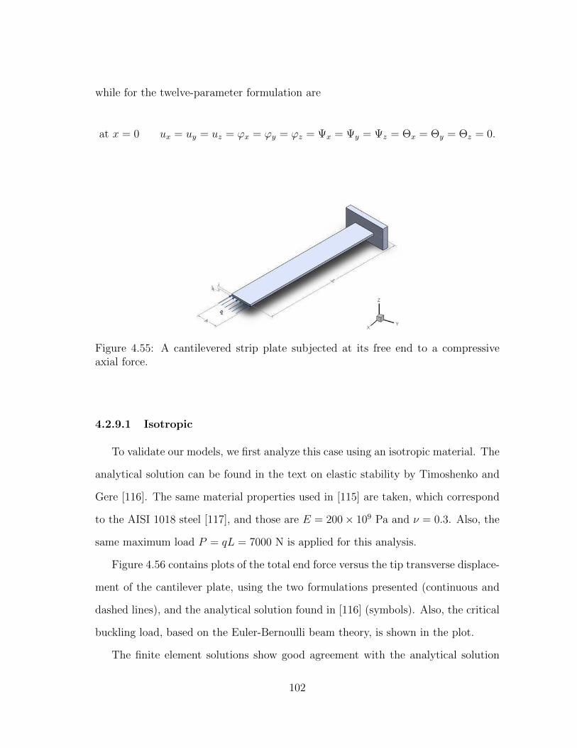
while for the twelve-parameter formulation are
at x = 0 ux = uy = uz = ϕx = ϕy = ϕz = Ψx = Ψy = Ψz = Θx = Θy = Θz = 0.
Figure 4.55: A cantilevered strip plate subjected at its free end to a compressiveaxial force.
4.2.9.1 Isotropic
To validate our models, we first analyze this case using an isotropic material. The
analytical solution can be found in the text on elastic stability by Timoshenko and
Gere [116]. The same material properties used in [115] are taken, which correspond
to the AISI 1018 steel [117], and those are E = 200× 109 Pa and ν = 0.3. Also, the
same maximum load P = qL = 7000 N is applied for this analysis.
Figure 4.56 contains plots of the total end force versus the tip transverse displace-
ment of the cantilever plate, using the two formulations presented (continuous and
dashed lines), and the analytical solution found in [116] (symbols). Also, the critical
buckling load, based on the Euler-Bernoulli beam theory, is shown in the plot.
The finite element solutions show good agreement with the analytical solution
102

and the ones reported by Arciniega and Reddy [22], and more recently by Payette
and Reddy [24]. We observe that both formulations predict the buckling. However,
the deformations are slightly different; the one obtained by means of the twelve-
parameter formulation presents greater deformation in the x direction, and lower
in the z direction, compared with the results obtained using the seven-parameter
formulation. We can see that the 12-parameter formulation has closer values to the
analytical solution. Figure 4.57 shows deformed configurations for various loads.
0 1 2 3 4 5 6 70
0.1
0.2
0.3
0.4
0.5
0.6
0.7
0.8
0.9
1
P (kN)
Defl
ecti
onat
the
tip
(m)
−uxuz
Critical load
Figure 4.56: Compressive load P vs. tip-deflection, for an isotropic cantilevered platestrip.
The maximum values of σxx are shown in Figure 4.58. The location where that
stresses are evaluated is included in the figure caption. We observe that the stresses
computed are slightly higher for the twelve-parameter formulation.
To show the capabilities of the presented formulations, we also compute other
forms of buckling, see Timoshenko and Gere [116]. In the previous works, only the
103
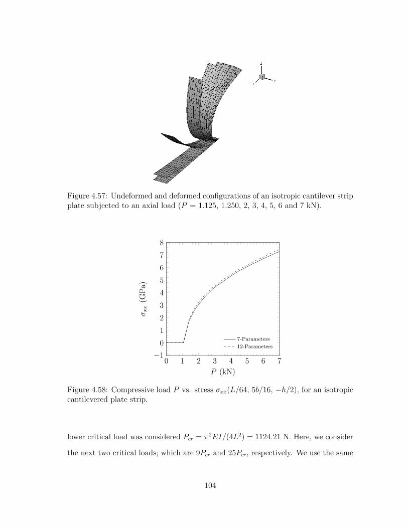
Figure 4.57: Undeformed and deformed configurations of an isotropic cantilever stripplate subjected to an axial load (P = 1.125, 1.250, 2, 3, 4, 5, 6 and 7 kN).
0 1 2 3 4 5 6 7−1
0
1
2
3
4
5
6
7
8
P (kN)
σxx
(GP
a)
7-Parameters
12-Parameters
Figure 4.58: Compressive load P vs. stress σxx(L/64, 5b/16, −h/2), for an isotropiccantilevered plate strip.
lower critical load was considered Pcr = π2EI/(4L2) = 1124.21 N. Here, we consider
the next two critical loads; which are 9Pcr and 25Pcr, respectively. We use the same
104
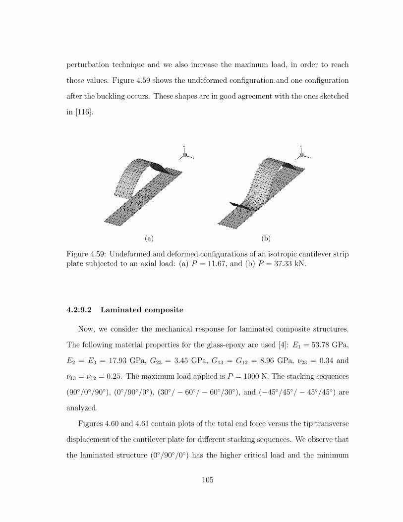
perturbation technique and we also increase the maximum load, in order to reach
those values. Figure 4.59 shows the undeformed configuration and one configuration
after the buckling occurs. These shapes are in good agreement with the ones sketched
in [116].
(a) (b)
Figure 4.59: Undeformed and deformed configurations of an isotropic cantilever stripplate subjected to an axial load: (a) P = 11.67, and (b) P = 37.33 kN.
4.2.9.2 Laminated composite
Now, we consider the mechanical response for laminated composite structures.
The following material properties for the glass-epoxy are used [4]: E1 = 53.78 GPa,
E2 = E3 = 17.93 GPa, G23 = 3.45 GPa, G13 = G12 = 8.96 GPa, ν23 = 0.34 and
ν13 = ν12 = 0.25. The maximum load applied is P = 1000 N. The stacking sequences
(90/0/90), (0/90/0), (30/ − 60/ − 60/30), and (−45/45/ − 45/45) are
analyzed.
Figures 4.60 and 4.61 contain plots of the total end force versus the tip transverse
displacement of the cantilever plate for different stacking sequences. We observe that
the laminated structure (0/90/0) has the higher critical load and the minimum
105

displacement in the x direction, while the laminate structure (90/0/90) has an
opposite behavior and the other two show intermediate response. Also, the laminate
structure (30/-60/-60/30) has the lower maximum displacement in the z direc-
tion, since it presents also displacement in the y direction due to the non-symmetrical
layers (see Figure 4.62).
0 200 400 600 800 1,000−0.8
−0.6
−0.4
−0.2
0
P (N)
Defl
ecti
onat
the
tip
(m)
(90/0/90)
(0/90/0)
(30/-60/-60/30)
(-45/45/-45/45)
Figure 4.60: Compressive load P vs. tip-deflection ux, for various laminated com-posite plates.
Figure 4.63 shows the maximum values of σxx for different laminated materials.
The location where those stresses are evaluated is included in the figure caption.
We observe that the stresses computed are, as in the isotropic case, slightly higher
for the twelve-parameter formulation. Furthermore, the maximum stress is found
in the stacking sequence (0/90/0), the same that has the lower deflection at the
tip, and the laminate structure (90/0/90) has the lower, while the others present
intermediate behavior.
106

0 200 400 600 800 1,0000
0.1
0.2
0.3
0.4
0.5
P (N)
Defl
ecti
onat
the
tip
(m)
(90/0/90)
(0/90/0)
(30/-60/-60/30)
(-45/45/-45/45)
Figure 4.61: Compressive load P vs. tip-deflection uz, for various laminated com-posite plates.
Figure 4.62: Deformed configuration of a laminated composite (30/-60/-60/30)cantilever strip plate subjected to an axial load (P = 1000 N).
4.2.9.3 Functionally graded
For functionally graded materials, we assume that the bottom surface (-) is 100%
aluminum and the top surface (+) is 100% zirconia. The material properties are
107

0 200 400 600 800 1,000
0
0.5
1
1.5
P
σxx(×
109)
(90/0/90)
(0/90/0)
(30/-60/-60/30)
(-45/45/-45/45)
Figure 4.63: Compressive load P vs. stress σxx(L/64, 5b/16, −h/2), for variouslaminated composite plates.
taken as [82]: E− = 70 × 109 Pa, E+ = 151 × 109 Pa, and ν = 0.3. The maximum
load applied is P = 7000 N.
Figures 4.64 and 4.65 contain plots of the total end force versus the tip dis-
placement in the x and z directions of the cantilever plate for various values of the
power-law index n. We find that the functionally graded response lies in between
that of the fully ceramic and that of the fully metal shells, being the latter the one
with a smaller critical load and maximum displacements in the x direction.
Figure 4.66 shows the maximum values of σxx for isotropic as well as functionally
graded cantilevered plate strips under compressive load P . The location where those
stresses are evaluated is included in the figure caption. We observe that the stresses
computed are, as in the previous cases, slightly higher for the twelve parameter
formulation. Furthermore, the maximum stress is found in the ceramic with modulus
E+, even when this structure experiences the lower deflection in the x direction. This
is due to the fact that the stresses are compared at the bottom surface, where the
108

0 1 2 3 4 5 6 7−0.9
−0.8
−0.7
−0.6
−0.5
−0.4
−0.3
−0.2
−0.1
0
P (kN)
Defl
ecti
onat
the
tip
(m)
Ceramic
n = 0.2
n = 0.5
n = 1.0
n = 2.0
n = 5.0
Metal
Figure 4.64: Compressive load P vs. tip-deflection ux, for various functionally gradedplates.
0 1 2 3 4 5 6 70
0.1
0.2
0.3
0.4
0.5
P (kN)
Defl
ecti
onat
the
tip
(m)
Ceramic
n = 0.2
n = 0.5
n = 1.0
n = 2.0
n = 5.0
Metal
Figure 4.65: Compressive load P vs. tip-deflection uz, for various functionally gradedplates.
109
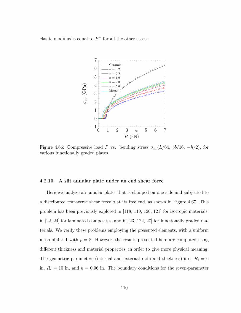
elastic modulus is equal to E− for all the other cases.
0 1 2 3 4 5 6 7−1
0
1
2
3
4
5
6
7
P (kN)
σxx
(GP
a)
Ceramic
n = 0.2
n = 0.5
n = 1.0
n = 2.0
n = 5.0
Metal
Figure 4.66: Compressive load P vs. bending stress σxx(L/64, 5b/16, −h/2), forvarious functionally graded plates.
4.2.10 A slit annular plate under an end shear force
Here we analyze an annular plate, that is clamped on one side and subjected to
a distributed transverse shear force q at its free end, as shown in Figure 4.67. This
problem has been previously explored in [118, 119, 120, 121] for isotropic materials,
in [22, 24] for laminated composites, and in [23, 122, 27] for functionally graded ma-
terials. We verify these problems employing the presented elements, with a uniform
mesh of 4 × 1 with p = 8. However, the results presented here are computed using
different thickness and material properties, in order to give more physical meaning.
The geometric parameters (internal and external radii and thickness) are: Ri = 6
in, Re = 10 in, and h = 0.06 in. The boundary conditions for the seven-parameter
110
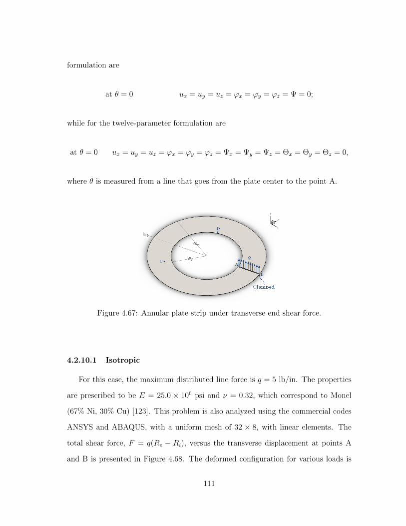
formulation are
at θ = 0 ux = uy = uz = ϕx = ϕy = ϕz = Ψ = 0;
while for the twelve-parameter formulation are
at θ = 0 ux = uy = uz = ϕx = ϕy = ϕz = Ψx = Ψy = Ψz = Θx = Θy = Θz = 0,
where θ is measured from a line that goes from the plate center to the point A.
Figure 4.67: Annular plate strip under transverse end shear force.
4.2.10.1 Isotropic
For this case, the maximum distributed line force is q = 5 lb/in. The properties
are prescribed to be E = 25.0 × 10⁶ psi and ν = 0.32, which correspond to Monel
(67% Ni, 30% Cu) [123]. This problem is also analyzed using the commercial codes
ANSYS and ABAQUS, with a uniform mesh of 32 × 8, with linear elements. The
total shear force, F = q(Re − Ri), versus the transverse displacement at points A
and B is presented in Figure 4.68. The deformed configuration for various loads is
111
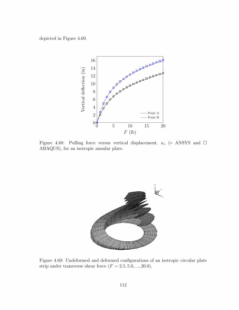
depicted in Figure 4.69.
0 5 10 15 200
2
4
6
8
10
12
14
16
F (lb)
Ver
tica
ldefl
ecti
on(i
n)
Point A
Point B
Figure 4.68: Pulling force versus vertical displacement, uz ( ANSYS and ABAQUS), for an isotropic annular plate.
Figure 4.69: Undeformed and deformed configurations of an isotropic circular platestrip under transverse shear force (F = 2.5, 5.0, ..., 20.0).
112
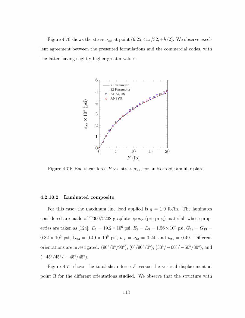
Figure 4.70 shows the stress σxx at point (6.25, 41π/32,+h/2). We observe excel-
lent agreement between the presented formulations and the commercial codes, with
the latter having slightly higher greater values.
0 5 10 15 200
1
2
3
4
5
6
F (lb)
σxx×
104
(psi
)7 Parameter
12 Parameter
ABAQUS
ANSYS
Figure 4.70: End shear force F vs. stress σxx, for an isotropic annular plate.
4.2.10.2 Laminated composite
For this case, the maximum line load applied is q = 1.0 lb/in. The laminates
considered are made of T300/5208 graphite-epoxy (pre-preg) material, whose prop-
erties are taken as [124]: E1 = 19.2×10⁶ psi, E2 = E3 = 1.56×10⁶ psi, G12 = G13 =
0.82 × 10⁶ psi, G23 = 0.49 × 10⁶ psi, ν12 = ν13 = 0.24, and ν23 = 0.49. Different
orientations are investigated: (90/0/90), (0/90/0), (30/−60/−60/30), and
(−45/45/− 45/45).
Figure 4.71 shows the total shear force F versus the vertical displacement at
point B for the different orientations studied. We observe that the structure with
113
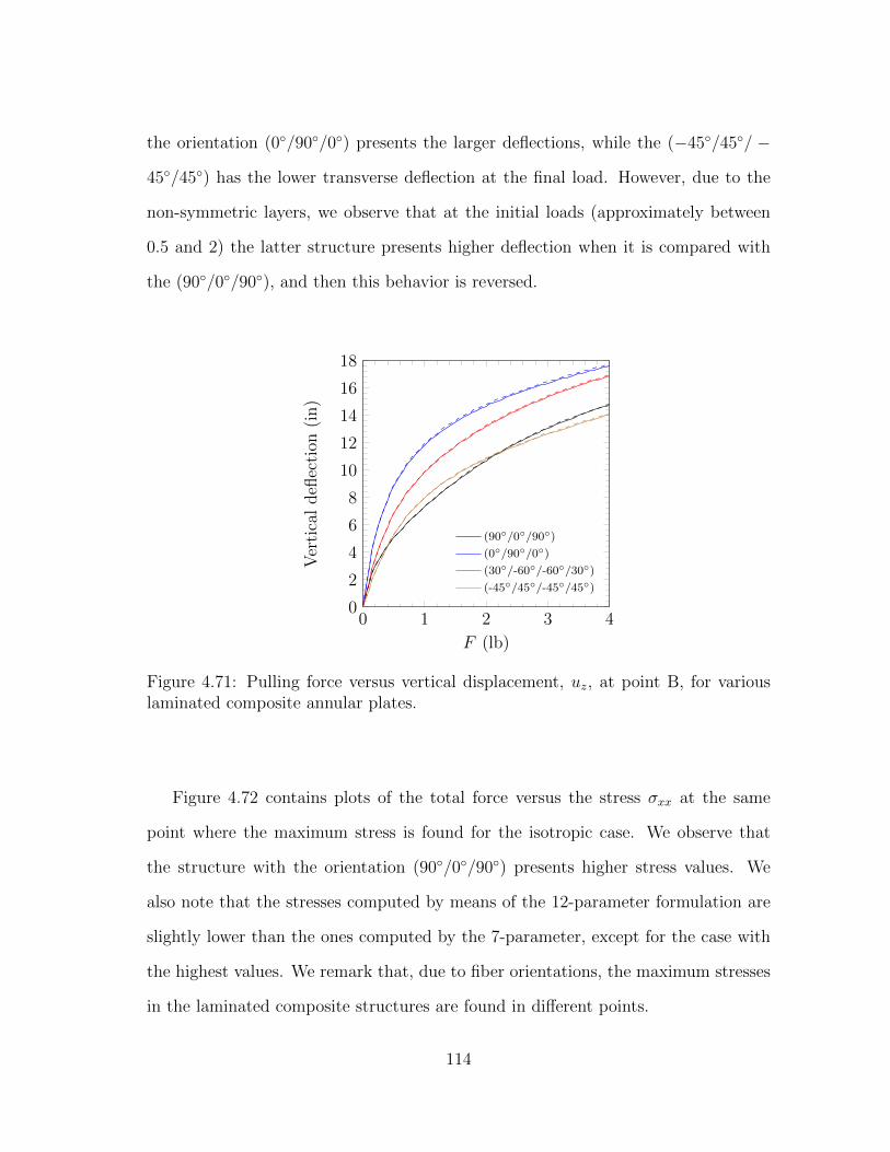
the orientation (0/90/0) presents the larger deflections, while the (−45/45/ −
45/45) has the lower transverse deflection at the final load. However, due to the
non-symmetric layers, we observe that at the initial loads (approximately between
0.5 and 2) the latter structure presents higher deflection when it is compared with
the (90/0/90), and then this behavior is reversed.
0 1 2 3 40
2
4
6
8
10
12
14
16
18
F (lb)
Ver
tica
ldefl
ecti
on(i
n)
(90/0/90)
(0/90/0)
(30/-60/-60/30)
(-45/45/-45/45)
Figure 4.71: Pulling force versus vertical displacement, uz, at point B, for variouslaminated composite annular plates.
Figure 4.72 contains plots of the total force versus the stress σxx at the same
point where the maximum stress is found for the isotropic case. We observe that
the structure with the orientation (90/0/90) presents higher stress values. We
also note that the stresses computed by means of the 12-parameter formulation are
slightly lower than the ones computed by the 7-parameter, except for the case with
the highest values. We remark that, due to fiber orientations, the maximum stresses
in the laminated composite structures are found in different points.
114
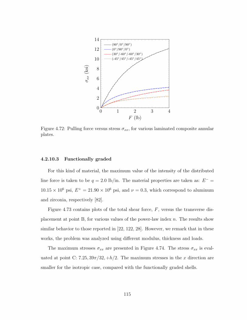
0 1 2 3 40
2
4
6
8
10
12
14
F (lb)
σxx
(ksi
)
(90/0/90)
(0/90/0)
(30/-60/-60/30)
(-45/45/-45/45)
Figure 4.72: Pulling force versus stress σxx, for various laminated composite annularplates.
4.2.10.3 Functionally graded
For this kind of material, the maximum value of the intensity of the distributed
line force is taken to be q = 2.0 lb/in. The material properties are taken as: E− =
10.15 × 10⁶ psi, E+ = 21.90 × 10⁶ psi, and ν = 0.3, which correspond to aluminum
and zirconia, respectively [82].
Figure 4.73 contains plots of the total shear force, F , versus the transverse dis-
placement at point B, for various values of the power-law index n. The results show
similar behavior to those reported in [22, 122, 28]. However, we remark that in these
works, the problem was analyzed using different modulus, thickness and loads.
The maximum stresses σxx are presented in Figure 4.74. The stress σxx is eval-
uated at point C: 7.25, 39π/32,+h/2. The maximum stresses in the x direction are
smaller for the isotropic case, compared with the functionally graded shells.
115
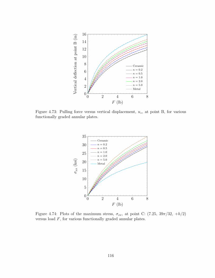
0 2 4 6 80
2
4
6
8
10
12
14
16
F (lb)
Ver
tica
ldefl
ecti
onat
poi
nt
B(i
n)
Ceramic
n = 0.2
n = 0.5
n = 1.0
n = 2.0
n = 5.0
Metal
Figure 4.73: Pulling force versus vertical displacement, uz, at point B, for variousfunctionally graded annular plates.
0 2 4 6 80
5
10
15
20
25
30
35
F (lb)
σxx
(ksi
)
Ceramic
n = 0.2
n = 0.5
n = 1.0
n = 2.0
n = 5.0
Metal
Figure 4.74: Plots of the maximum stress, σxx, at point C: (7.25, 39π/32, +h/2)versus load F , for various functionally graded annular plates.
116
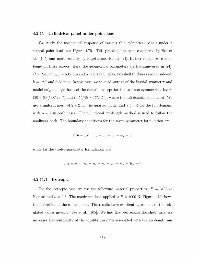
4.2.11 Cylindrical panel under point load
We study the mechanical response of various thin cylindrical panels under a
central point load, see Figure 4.75. This problem has been considered by Sze et
al. [105] and more recently by Payette and Reddy [24], further references can be
found on these papers. Here, the geometrical parameters are the same used in [24]:
R = 2540 mm, a = 508 mm and α = 0.1 rad. Also, two shell thickness are considered:
h = 12.7 and 6.35 mm. In this case, we take advantage of the biaxial symmetry and
model only one quadrant of the domain; except for the two non symmetrical layers
(30/-60/-60/30) and (-45/45/-45/45), where the full domain is modeled. We
use a uniform mesh of 2 × 2 for the quarter model and a 4 × 4 for the full domain,
with p = 4 in both cases. The cylindrical arc-length method is used to follow the
nonlinear path. The boundary conditions for the seven-parameter formulation are
at θ = ±α ux = uy = uz = ϕx = 0;
while for the twelve-parameter formulation are
at θ = ±α ux = uy = uz = ϕx = Ψx = Θx = 0.
4.2.11.1 Isotropic
For the isotropic case, we use the following material properties: E = 3102.75
N/mm2 and ν = 0.3. The maximum load applied is P = 4000 N. Figure 4.76 shows
the deflection at the center point. The results have excellent agreement to the tab-
ulated values given by Sze et al. [105]. We find that decreasing the shell thickness
increases the complexity of the equilibrium path associated with the arc-length nu-
117
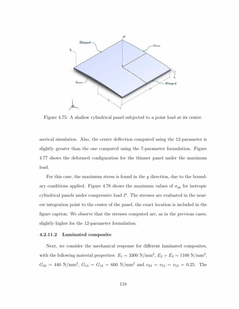
Figure 4.75: A shallow cylindrical panel subjected to a point load at its center.
merical simulation. Also, the center deflection computed using the 12-parameter is
slightly greater than the one computed using the 7-parameter formulation. Figure
4.77 shows the deformed configuration for the thinner panel under the maximum
load.
For this case, the maximum stress is found in the y direction, due to the bound-
ary conditions applied. Figure 4.78 shows the maximum values of σyy for isotropic
cylindrical panels under compressive load P . The stresses are evaluated in the near-
est integration point to the center of the panel, the exact location is included in the
figure caption. We observe that the stresses computed are, as in the previous cases,
slightly higher for the 12-parameter formulation.
4.2.11.2 Laminated composite
Next, we consider the mechanical response for different laminated composites,
with the following material properties: E1 = 3300 N/mm2, E2 = E3 = 1100 N/mm2,
G23 = 440 N/mm2, G13 = G12 = 660 N/mm2 and ν23 = ν13 = ν12 = 0.25. The
118

−1 0 1 2 3 40
5
10
15
20
25
30
35
40
45
Point load (kN)Defl
ecti
onat
the
cente
rof
the
pan
el(m
m)
12.7 mm, 7P
6.35 mm, 7P
12.7 mm, 12P
6.35 mm, 12P
Figure 4.76: Vertical deflection of isotropic shallow cylindrical panels under pointloading.
Figure 4.77: Deformed configuration of an isotropic cylindrical panel, h = 6.35 mmand P = 4000 N.
stacking sequences (90/0/90), (0/90/0), (30/-60/-60/30), and (-45/45/-
45/45) are analyzed.
Figures 4.79 and 4.80 show plots of the point force versus the center vertical
119

−1 0 1 2 3 4−10
0
10
20
30
40
50
60
70
Point load (kN)
σyy
(MP
a)
12.7 mm, 7P
6.35 mm, 7P
12.7 mm, 12P
6.35 mm, 12P
Figure 4.78: Point load P vs. stress σyy(R−h/2, π/160, 15a/32) of isotropic shallowcylindrical panels under point loading.
deflection, for different values of h and different stacking sequences, with excellent
agreement to the solutions presented by Arciniega and Reddy [22], and more recently
by Payette and Reddy [24]. We observe that the laminated structure (0/90/0)
has the maximum displacement, while the laminate structure (90/0/90) has the
minimum and the other two show intermediate response.
Figures 4.81 and 4.82 show the maximum values of σyy for laminated composite
cylindrical panels under compressive load P . The location where that stresses are
evaluated is included in the figure caption. For these stacking sequences, the laminate
(90/0/90) shows the maximum stress, while the (0/90/0) has the minimum and
the other two present intermediate behavior. We remark that, due to the fiber orien-
tations, the maximum stress for the structures considered here is in the y direction,
except for the (0/90/0) stacking sequence where its maximum stress occurs in the
x direction.
120

−0.5 0 0.5 1 1.5 2 2.5 3 3.5 40
5
10
15
20
25
30
35
40
45
Point load (kN)Defl
ecti
onat
the
cente
rof
the
pan
el(m
m)
(90/0/90)
(0/90/0)
(30/-60/-60/30)
(-45/45/-45/45)
Figure 4.79: Vertical deflection of laminated composite shallow cylindrical panelsunder point loading, h = 12.7 mm.
−0.5 0 0.5 1 1.5 2 2.5 3 3.5 40
5
10
15
20
25
30
35
40
45
50
Point load (kN)Defl
ecti
onat
the
cente
rof
the
pan
el(m
m)
(90/0/90)
(0/90/0)
(30/-60/-60/30)
(-45/45/-45/45)
Figure 4.80: Vertical deflection of laminated composite shallow cylindrical panelsunder point loading, h = 6.35 mm.
121
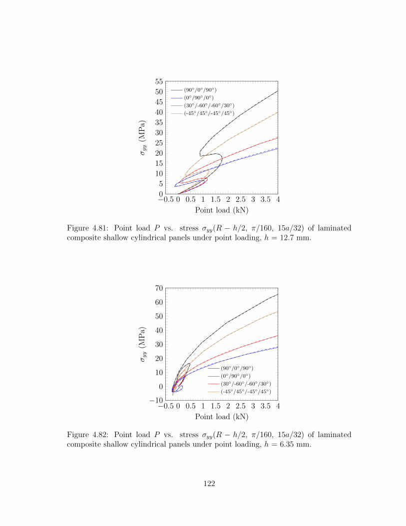
−0.5 0 0.5 1 1.5 2 2.5 3 3.5 40
5
10
15
20
25
30
35
40
45
50
55
Point load (kN)
σyy
(MP
a)
(90/0/90)
(0/90/0)
(30/-60/-60/30)
(-45/45/-45/45)
Figure 4.81: Point load P vs. stress σyy(R − h/2, π/160, 15a/32) of laminatedcomposite shallow cylindrical panels under point loading, h = 12.7 mm.
−0.5 0 0.5 1 1.5 2 2.5 3 3.5 4−10
0
10
20
30
40
50
60
70
Point load (kN)
σyy
(MP
a)
(90/0/90)
(0/90/0)
(30/-60/-60/30)
(-45/45/-45/45)
Figure 4.82: Point load P vs. stress σyy(R − h/2, π/160, 15a/32) of laminatedcomposite shallow cylindrical panels under point loading, h = 6.35 mm.
122
4.2.11.3 Functionally graded
For functionally graded materials, we use the following material properties: E− =
70 × 103 N/mm2, E+ = 151 × 103 N/mm2, and ν = 0.3. The maximum loads used
are P = 400 kN for h = 12.7 mm, and P = 220 kN for h = 6.35 mm.
Figures 4.83 and 4.84 contain plots of the point force P versus the tip central
deflection for various values of the power-law index n, with excellent agreement to
the solutions presented by Arciniega and Reddy [22], and more recently by Payette
and Reddy [24]. We find that the functionally graded response lies in between that
of the fully ceramic and those of the fully metal shells, being the latter the one with
the maximum displacement.
0 100 200 300 4000
5
10
15
20
25
30
35
40
45
Point load (kN)Defl
ecti
onat
the
cente
rof
the
pan
el(m
m)
Ceramic
n = 0.2
n = 0.5
n = 1.0
n = 2.0
n = 5.0
Metal
Figure 4.83: Vertical deflection of functionally graded shallow cylindrical panels un-der point loading, h = 12.7 mm.
Figures 4.85 and 4.86 show the maximum values of σyy for isotropic as well as
123
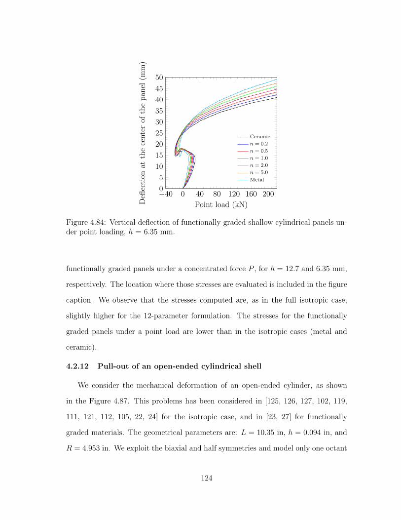
−40 0 40 80 120 160 2000
5
10
15
20
25
30
35
40
45
50
Point load (kN)Defl
ecti
onat
the
cente
rof
the
pan
el(m
m)
Ceramic
n = 0.2
n = 0.5
n = 1.0
n = 2.0
n = 5.0
Metal
Figure 4.84: Vertical deflection of functionally graded shallow cylindrical panels un-der point loading, h = 6.35 mm.
functionally graded panels under a concentrated force P , for h = 12.7 and 6.35 mm,
respectively. The location where those stresses are evaluated is included in the figure
caption. We observe that the stresses computed are, as in the full isotropic case,
slightly higher for the 12-parameter formulation. The stresses for the functionally
graded panels under a point load are lower than in the isotropic cases (metal and
ceramic).
4.2.12 Pull-out of an open-ended cylindrical shell
We consider the mechanical deformation of an open-ended cylinder, as shown
in the Figure 4.87. This problems has been considered in [125, 126, 127, 102, 119,
111, 121, 112, 105, 22, 24] for the isotropic case, and in [23, 27] for functionally
graded materials. The geometrical parameters are: L = 10.35 in, h = 0.094 in, and
R = 4.953 in. We exploit the biaxial and half symmetries and model only one octant
124

0 100 200 300 4000
0.5
1
1.5
2
2.5
3
3.5
Point load (kN)
σyy
(GP
a)
Ceramic
n = 0.2
n = 0.5
n = 1.0
n = 2.0
n = 5.0
Metal
Figure 4.85: Point load P versus stress σyy(R− h/2, π/160, 15a/32) of functionallygraded shallow cylindrical panels under point loading, h = 12.7 mm.
−40 0 40 80 120 160 200−0.5
0
0.5
1
1.5
2
2.5
3
3.5
Point load (kN)
σyy
(GP
a)
Ceramic
n = 0.2
n = 0.5
n = 1.0
n = 2.0
n = 5.0
Metal
Figure 4.86: Point load P versus stress σyy(R− h/2, π/160, 15a/32) of functionallygraded shallow cylindrical panels under point loading, h = 6.35 mm.
125

of the shell, using a uniform mesh of 2× 2 with p = 8 for the formulations presented
here, and a uniform mesh of 16× 16 for the commercial codes with linear elements.
Figure 4.87: Pull-out of a cylinder with free edges.
4.2.12.1 Isotropic
For this case, the properties are prescribed to be: E = 10.5×10⁶ psi, ν = 0.3125,
which correspond to typical values for an aluminum alloy [117]. The maximum load
applied is taken as P = 4× 10⁴ lb. Figure 4.88 shows the radial defection versus the
net applied pulling force P at points A, B and C (see Figure 4.87). We observe that
there is a very good agreement in the results, specially between the 12-parameter
formulation and the commercial codes in the bifurcation paths at points B and C.
Figures 4.89 and 4.90 show the maximum stress σxx and σzz, respectively, at
the nearest integration point to the applied load (R + h/2, π/64, 31L/64). We
observe that there is a difference between the two formulations presented here in
the values of the stresses, but a similar path. The results obtained by means of
the commercial codes are considerably higher than the ones computed using the
126
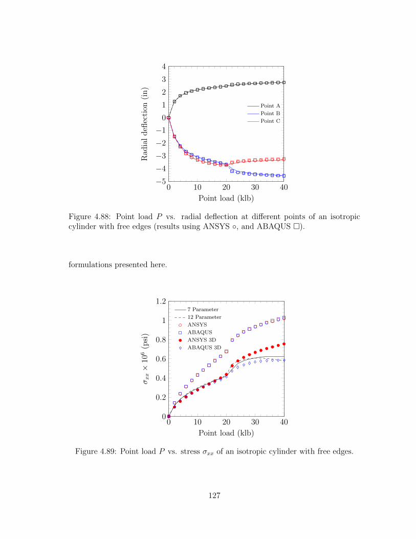
0 10 20 30 40−5
−4
−3
−2
−1
0
1
2
3
4
Point load (klb)
Rad
ial
defl
ecti
on(i
n)
Point A
Point B
Point C
Figure 4.88: Point load P vs. radial deflection at different points of an isotropiccylinder with free edges (results using ANSYS , and ABAQUS ).
formulations presented here.
0 10 20 30 400
0.2
0.4
0.6
0.8
1
1.2
Point load (klb)
σxx×
106
(psi
)
7 Parameter
12 Parameter
ANSYS
ABAQUS
ANSYS 3D
ABAQUS 3D
Figure 4.89: Point load P vs. stress σxx of an isotropic cylinder with free edges.
127
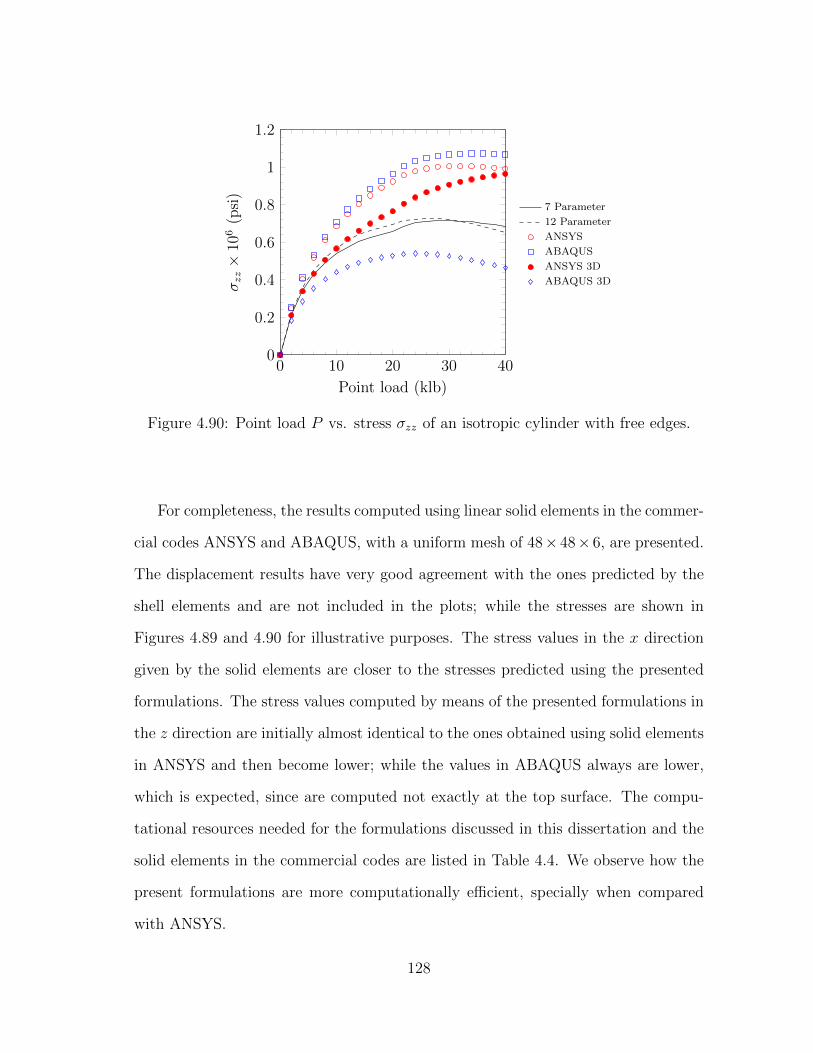
0 10 20 30 400
0.2
0.4
0.6
0.8
1
1.2
Point load (klb)
σzz×
106
(psi
)
7 Parameter
12 Parameter
ANSYS
ABAQUS
ANSYS 3D
ABAQUS 3D
Figure 4.90: Point load P vs. stress σzz of an isotropic cylinder with free edges.
For completeness, the results computed using linear solid elements in the commer-
cial codes ANSYS and ABAQUS, with a uniform mesh of 48× 48× 6, are presented.
The displacement results have very good agreement with the ones predicted by the
shell elements and are not included in the plots; while the stresses are shown in
Figures 4.89 and 4.90 for illustrative purposes. The stress values in the x direction
given by the solid elements are closer to the stresses predicted using the presented
formulations. The stress values computed by means of the presented formulations in
the z direction are initially almost identical to the ones obtained using solid elements
in ANSYS and then become lower; while the values in ABAQUS always are lower,
which is expected, since are computed not exactly at the top surface. The compu-
tational resources needed for the formulations discussed in this dissertation and the
solid elements in the commercial codes are listed in Table 4.4. We observe how the
present formulations are more computationally efficient, specially when compared
with ANSYS.
128
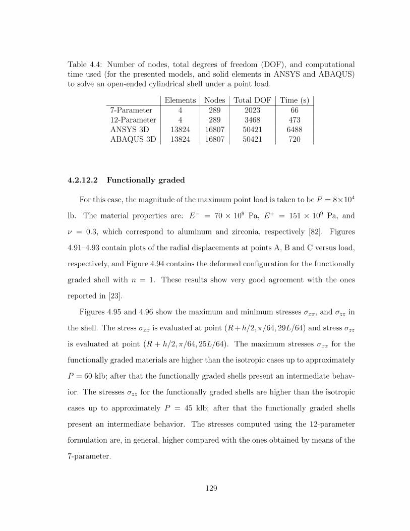
Table 4.4: Number of nodes, total degrees of freedom (DOF), and computationaltime used (for the presented models, and solid elements in ANSYS and ABAQUS)to solve an open-ended cylindrical shell under a point load.
Elements Nodes Total DOF Time (s)7-Parameter 4 289 2023 6612-Parameter 4 289 3468 473ANSYS 3D 13824 16807 50421 6488ABAQUS 3D 13824 16807 50421 720
4.2.12.2 Functionally graded
For this case, the magnitude of the maximum point load is taken to be P = 8×10⁴
lb. The material properties are: E− = 70 × 109 Pa, E+ = 151 × 109 Pa, and
ν = 0.3, which correspond to aluminum and zirconia, respectively [82]. Figures
4.91–4.93 contain plots of the radial displacements at points A, B and C versus load,
respectively, and Figure 4.94 contains the deformed configuration for the functionally
graded shell with n = 1. These results show very good agreement with the ones
reported in [23].
Figures 4.95 and 4.96 show the maximum and minimum stresses σxx, and σzz in
the shell. The stress σxx is evaluated at point (R+h/2, π/64, 29L/64) and stress σzz
is evaluated at point (R + h/2, π/64, 25L/64). The maximum stresses σxx for the
functionally graded materials are higher than the isotropic cases up to approximately
P = 60 klb; after that the functionally graded shells present an intermediate behav-
ior. The stresses σzz for the functionally graded shells are higher than the isotropic
cases up to approximately P = 45 klb; after that the functionally graded shells
present an intermediate behavior. The stresses computed using the 12-parameter
formulation are, in general, higher compared with the ones obtained by means of the
7-parameter.
129
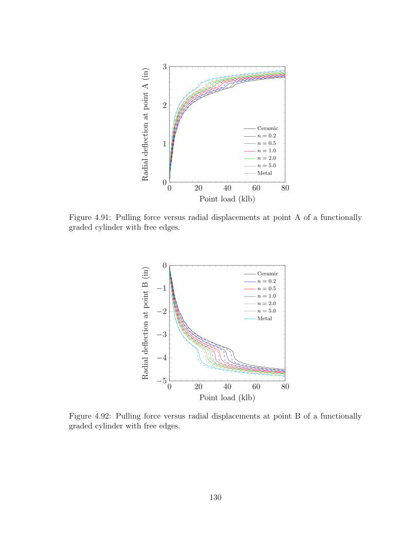
0 20 40 60 800
1
2
3
Point load (klb)
Rad
ial
defl
ecti
onat
poi
nt
A(i
n)
Ceramic
n = 0.2
n = 0.5
n = 1.0
n = 2.0
n = 5.0
Metal
Figure 4.91: Pulling force versus radial displacements at point A of a functionallygraded cylinder with free edges.
0 20 40 60 80−5
−4
−3
−2
−1
0
Point load (klb)
Rad
ial
defl
ecti
onat
poi
nt
B(i
n)
Ceramic
n = 0.2
n = 0.5
n = 1.0
n = 2.0
n = 5.0
Metal
Figure 4.92: Pulling force versus radial displacements at point B of a functionallygraded cylinder with free edges.
130

0 20 40 60 80−4
−3
−2
−1
0
Point load (klb)
Rad
ial
defl
ecti
onat
poi
nt
C(i
n)
Ceramic
n = 0.2
n = 0.5
n = 1.0
n = 2.0
n = 5.0
Metal
Figure 4.93: Pulling force versus radial displacements at point C of a functionallygraded cylinder with free edges.
Figure 4.94: Deformed configuration of the functionally graded cylindrical shell underpulling forces. Load P = 5× 10⁶ and n = 1.0.
4.2.13 A pinched half-cylindrical shell
We consider a half-cylindrical shell subjected to a single point force P as shown
in Figure 4.97. This problem has been considered in [128, 129, 105, 22, 24]. The
131

0 20 40 60 800
0.2
0.4
0.6
0.8
1
1.2
Point load (klb)
σxx×
106
(psi
)
Ceramic
n = 0.2
n = 0.5
n = 1.0
n = 2.0
n = 5.0
Metal
Figure 4.95: Plots of the maximum stress, σxx(R + h/2, π/64, 29L/64) versus loadP of a functionally graded cylinder with free edges.
0 20 40 60 800
0.5
1
1.5
Point load (klb)
σzz×
106
(psi
)
Ceramic
n = 0.2
n = 0.5
n = 1.0
n = 2.0
n = 5.0
Metal
Figure 4.96: Plots of the maximum stress, σzz(R + h/2, π/64, 25L/64) versus loadP of a functionally graded cylinder with free edges.
geometrical parameters are: L = 304.8 mm, R = 101.6 mm, and h = 3 mm. We
exploit symmetry and model only half of the domain, using a uniform mesh of 4× 4
132
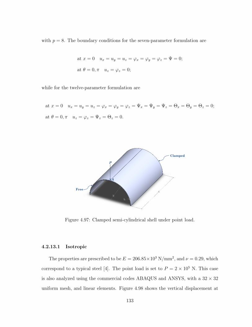
with p = 8. The boundary conditions for the seven-parameter formulation are
at x = 0 ux = uy = uz = ϕx = ϕy = ϕz = Ψ = 0;
at θ = 0, π uz = ϕz = 0;
while for the twelve-parameter formulation are
at x = 0 ux = uy = uz = ϕx = ϕy = ϕz = Ψx = Ψy = Ψz = Θx = Θy = Θz = 0;
at θ = 0, π uz = ϕz = Ψz = Θz = 0.
Free
Clamped
P
A
Figure 4.97: Clamped semi-cylindrical shell under point load.
4.2.13.1 Isotropic
The properties are prescribed to be E = 206.85×10³ N/mm2, and ν = 0.29, which
correspond to a typical steel [4]. The point load is set to P = 2 × 10⁵ N. This case
is also analyzed using the commercial codes ABAQUS and ANSYS, with a 32 × 32
uniform mesh, and linear elements. Figure 4.98 shows the vertical displacement at
133
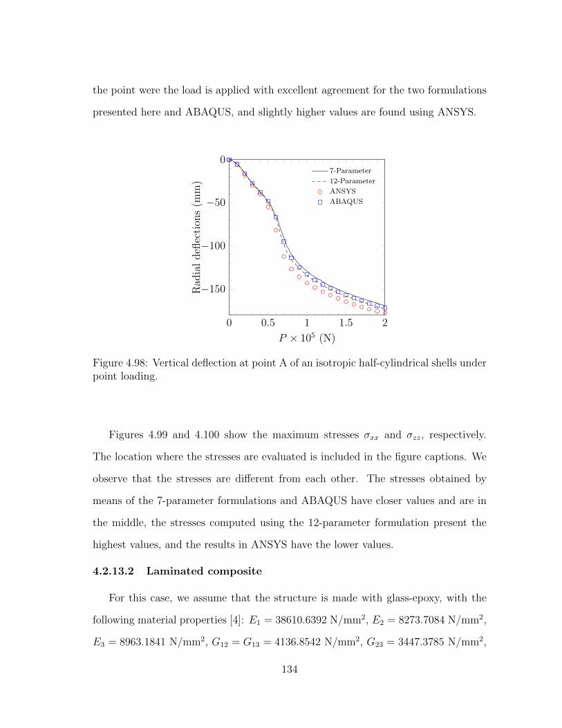
the point were the load is applied with excellent agreement for the two formulations
presented here and ABAQUS, and slightly higher values are found using ANSYS.
0 0.5 1 1.5 2
−150
−100
−50
0
P × 105 (N)
Rad
ial
defl
ecti
ons
(mm
)
7-Parameter
12-Parameter
ANSYS
ABAQUS
Figure 4.98: Vertical deflection at point A of an isotropic half-cylindrical shells underpoint loading.
Figures 4.99 and 4.100 show the maximum stresses σxx and σzz, respectively.
The location where the stresses are evaluated is included in the figure captions. We
observe that the stresses are different from each other. The stresses obtained by
means of the 7-parameter formulations and ABAQUS have closer values and are in
the middle, the stresses computed using the 12-parameter formulation present the
highest values, and the results in ANSYS have the lower values.
4.2.13.2 Laminated composite
For this case, we assume that the structure is made with glass-epoxy, with the
following material properties [4]: E1 = 38610.6392 N/mm2, E2 = 8273.7084 N/mm2,
E3 = 8963.1841 N/mm2, G12 = G13 = 4136.8542 N/mm2, G23 = 3447.3785 N/mm2,
134
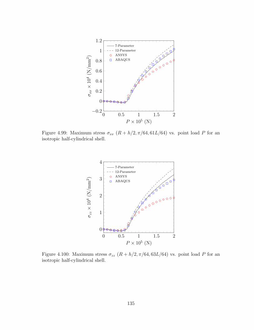
0 0.5 1 1.5 2−0.2
0
0.2
0.4
0.6
0.8
1
1.2
P × 105 (N)
σxx×
104
(N/m
m2)
7-Parameter
12-Parameter
ANSYS
ABAQUS
Figure 4.99: Maximum stress σxx (R + h/2, π/64, 61L/64) vs. point load P for anisotropic half-cylindrical shell.
0 0.5 1 1.5 2
0
1
2
3
4
P × 105 (N)
σzz×
104
(N/m
m2)
7-Parameter
12-Parameter
ANSYS
ABAQUS
Figure 4.100: Maximum stress σzz (R + h/2, π/64, 63L/64) vs. point load P for anisotropic half-cylindrical shell.
135

ν12 = ν13 = 0.26, and ν23 = 0.34. The maximum load applied is P = 2 × 10⁴ N.
Different orientations are investigated: (90/0/90), and (0/90/0). Again, the
results are compared with the commercial codes ANSYS and ABAQUS with the
same mesh and elements used for the isotropic case.
Figure 4.101 shows the vertical deflection at point A versus the point load P .
We observe good agreement between the formulations presented here and ABAQUS,
being the 12-Parameter the one with higher values. On the other hand ANSYS differs
considerably, specially for the configuration (90/0/90), from the others presenting
higher values. We observe that the structure (0/90/0) has higher deflection, under
the same load for this structure. Figure 4.102 presents the deformed configuration
of the laminated structure (90/0/90) at the maximum load.
0 0.5 1 1.5 2−200
−150
−100
−50
0
P × 104 (N)
Rad
ial
defl
ecti
ons
(mm
)
7-Parameter
12-Parameter
ANSYS
ABAQUS
Figure 4.101: Vertical deflection at point A for a (90/0/90) and (0/90/0) lami-nated composite half-cylindrical shells under point loading, represented by black andblue lines, respectively.
136

Figure 4.102: Deformed configuration of a laminated composited pinched half cylin-drical shell (90/0/90) for P = 2× 10⁴ N.
Figures 4.103 and 4.104 show the maximum stress σzz for the stacking sequences
considered, (90/0/90) and (0/90/0), where different behaviors are observed.
On one hand, the formulations presented here have higher values, specially the 12-
parameter formulation, with the same trend. On the other hand, the commercial
codes differ from each other, having ABAQUS a similar behavior to the results
presented here and ANSYS showing a similar trend after the breaking point for the
(90/0/90) and a totally different one for the (0/90/0).
4.2.14 A pinched hemisphere with an 18 hole
We consider the problem proposed by MacNeal and Harder [130] to test doubly-
curved shells, a pinched isotropic hemisphere with an 18 circular cutout. This
problem has been considered by many other authors, see for example [107, 131, 118,
126, 127, 53, 102, 103, 132, 111, 133, 105, 24]. The external loads for the problem
consist of four alternating radial point forces P , prescribed along the equator at
90 intervals (see Figure 4.105). Due to the symmetry, only one quarter of the
137
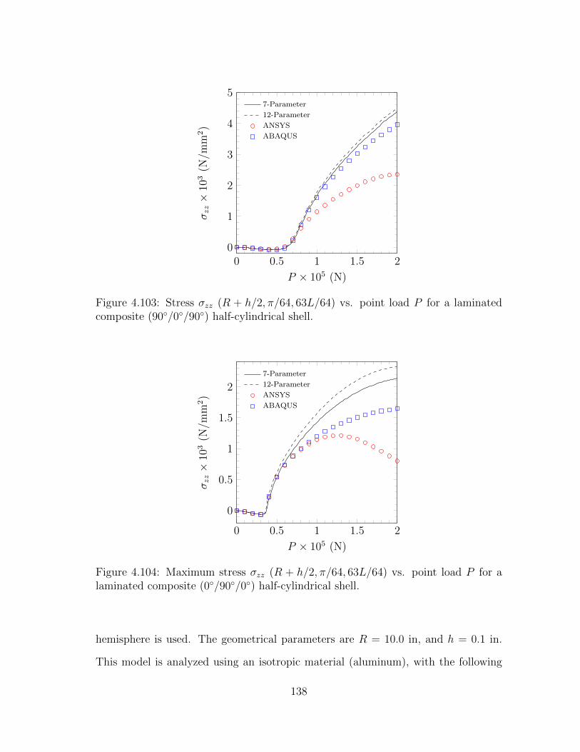
0 0.5 1 1.5 20
1
2
3
4
5
P × 105 (N)
σzz×
103
(N/m
m2)
7-Parameter
12-Parameter
ANSYS
ABAQUS
Figure 4.103: Stress σzz (R + h/2, π/64, 63L/64) vs. point load P for a laminatedcomposite (90/0/90) half-cylindrical shell.
0 0.5 1 1.5 2
0
0.5
1
1.5
2
P × 105 (N)
σzz×
103
(N/m
m2)
7-Parameter
12-Parameter
ANSYS
ABAQUS
Figure 4.104: Maximum stress σzz (R + h/2, π/64, 63L/64) vs. point load P for alaminated composite (0/90/0) half-cylindrical shell.
hemisphere is used. The geometrical parameters are R = 10.0 in, and h = 0.1 in.
This model is analyzed using an isotropic material (aluminum), with the following
138
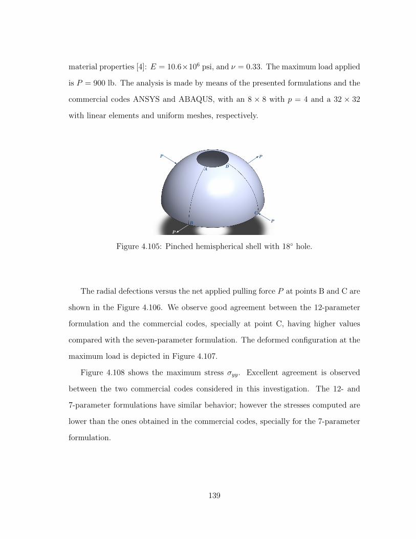
material properties [4]: E = 10.6×10⁶ psi, and ν = 0.33. The maximum load applied
is P = 900 lb. The analysis is made by means of the presented formulations and the
commercial codes ANSYS and ABAQUS, with an 8 × 8 with p = 4 and a 32 × 32
with linear elements and uniform meshes, respectively.
P
P P
P
C
D
B
A
Figure 4.105: Pinched hemispherical shell with 18 hole.
The radial defections versus the net applied pulling force P at points B and C are
shown in the Figure 4.106. We observe good agreement between the 12-parameter
formulation and the commercial codes, specially at point C, having higher values
compared with the seven-parameter formulation. The deformed configuration at the
maximum load is depicted in Figure 4.107.
Figure 4.108 shows the maximum stress σyy. Excellent agreement is observed
between the two commercial codes considered in this investigation. The 12- and
7-parameter formulations have similar behavior; however the stresses computed are
lower than the ones obtained in the commercial codes, specially for the 7-parameter
formulation.
139

0 1 2 3 4 5 6 7 8 90
1
2
3
4
5
6
7
8
9
P × 102 (lb)
Rad
ial
defl
ecti
ons
(in)
Point B
Point C
Figure 4.106: Radial deflections at points B and C of the pinched hemisphere (ABAQUS, and ANSYS).
Figure 4.107: Deformed configuration of a pinched hemispherical shell for P = 900lb.
140

0 1 2 3 4 5 6 7 8 90
1
2
3
4
5
P × 102 (lb)
σyy×
105
(psi
)7-Parameter
12-Parameter
ANSYS
ABAQUS
Figure 4.108: Pulling force P versus stress σyy of the pinched hemisphere.
4.2.15 A pinched composite hyperboloidal shell
Finally, we consider the finite deformation of a laminated composite hyperboloidal
shell that is loaded by four alternating radial point forces P (see Figure 4.109). This
problem has been considered in [134, 135, 136, 137, 22, 24]. The geometric parameters
are taken as R1 = 7.5 m, R2 = 15.0 m, L = 20.0 m, and h = 0.04 m. The coordinates
of the intermediate radius are computed by
R(z) = R1
√1 + (z/C)2 (4.34)
where C = 20/√
3.
The material properties are taken from [134], which correspond to: E1 = 40.0×
106 kN/m2, E2 = E3 = 1.0 × 10⁶ kN/m2, G12 = G13 = G23 = 0.6 × 10⁶ kN/m2,
and ν12 = ν13 = ν23 = 0.25. Two different stacking sequences are investigated:
(90/0/90), and (0/90/0). In both cases, the maximum load applied is P = 600
141

P
P P
P
A B
C D
Figure 4.109: Hyperboloidal shell.
kN. Due to the symmetry, only one octant of the domain is modeled. This problem
is studied using the presented formulations with a 4 × 4 uniform mesh, with p = 8,
and the commercial codes ANSYS and ABAQUS with a 32× 32 regular mesh, with
linear elements.
Radial defections at points A, B, C and D versus the applied pulling force P
are shown in the Figures 4.110 and 4.111, for the (0/90/0) and (90/0/90)
staking sequences, respectively. We observe good agreement for the first composite
structure and some differences between the commercial codes and the formulations
presented here for the second case at points A and C. Figure 4.112 shows the deformed
configuration for the (90/0/90) structure when P = 480.
Figures 4.113 and 4.114 show the maximum stresses for the (0/90/0) and
(90/0/90) staking sequences, respectively. In the first case, the maximum stress is
located in the y direction, and we observe good agreement between all formulations
at the begging (P < 100 kN) and then a difference between them, with lower values
142
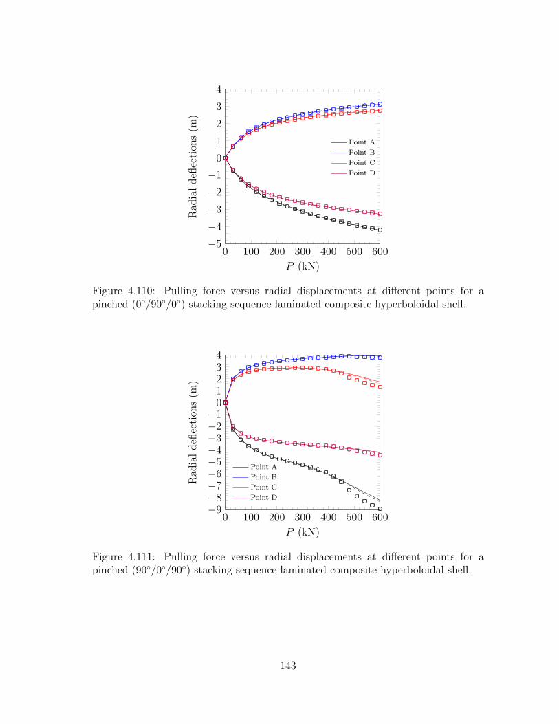
0 100 200 300 400 500 600−5
−4
−3
−2
−1
0
1
2
3
4
P (kN)
Rad
ial
defl
ecti
ons
(m)
Point A
Point B
Point C
Point D
Figure 4.110: Pulling force versus radial displacements at different points for apinched (0/90/0) stacking sequence laminated composite hyperboloidal shell.
0 100 200 300 400 500 600−9−8−7−6−5−4−3−2−1
01234
P (kN)
Rad
ial
defl
ecti
ons
(m)
Point A
Point B
Point C
Point D
Figure 4.111: Pulling force versus radial displacements at different points for apinched (90/0/90) stacking sequence laminated composite hyperboloidal shell.
143
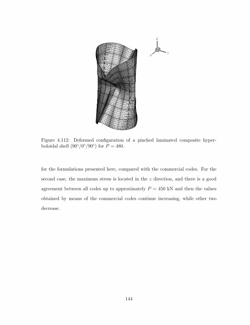
Figure 4.112: Deformed configuration of a pinched laminated composite hyper-boloidal shell (90/0/90) for P = 480.
for the formulations presented here, compared with the commercial codes. For the
second case, the maximum stress is located in the z direction, and there is a good
agreement between all codes up to approximately P = 450 kN and then the values
obtained by means of the commercial codes continue increasing, while other two
decrease.
144

0 100 200 300 400 500 6000
0.2
0.4
0.6
0.8
1
1.2
1.4
1.6
P (kN)
σyy×
105
(kN
/m2)
7-Parameter
12-Parameter
ANSYS
ABAQUS
Figure 4.113: Pulling force versus the stress σyy for the (0/90/0) stacking sequence.
0 100 200 300 400 500 6000
1
2
3
4
5
6
7
8
9
P (kN)
σzz×
105
(kN
/m2)
7-Parameter
12-Parameter
ANSYS
ABAQUS
Figure 4.114: Pulling force versus the stress σzz for the (90/0/90) stacking se-quence.
145
5. TRANSIENT ANALYSIS
In this chapter, we develop the finite element models of time-dependent problems
for the shell elements presented in Chapter 3, using Newmark’s scheme. General as-
pects about its implementation and how to obtain the fully discretized equations are
given. Furthermore, numerical results for different problems are presented, to prove
the advantages of the implemented formulations. The transient response of isotropic,
laminated composite and functionally graded plates, cylindrical and spherical shells
is studied. The importance of the shell thickness and the kinematics assumed in the
thickness direction for transient analysis is shown.
5.1 Finite element model
Substituting the finite element approximation of the displacement fields given in
Equation (4.1) for the seven-parameter, or Equation (4.4) for the twelve-parameter
formulation, into the Euler-Lagrange equations we obtain the second-order equation
[M]∆+ [K(∆)]∆ = F (5.1)
where [M] is the mass matrix, and [K(∆)] is the stiffness matrix. Note that the
stiffness matrix is function of the displacements, while the mass matrix is independent
of them. The global displacement vector ∆ is subjected to the initial conditions
in which the displacement and velocity fields are known at time t = 0. In this work,
we assume that they are equal to zero.
We use the method proposed by Newmark [138] to solve this problem. He assumed
146
that the function and its time derivatives can be approximated by
∆s+1 = ∆s + ∆t∆s +1
2(∆t)2∆s+γ
∆s+1 = ∆s + ∆s+α∆t
∆s+α = (1− α)∆s + α∆s+1 (5.2)
where α and γ are parameters that determine the stability and accuracy of the
scheme. In this work, we use the constant-average acceleration method, which cor-
responds to the case where α = 0.5, and γ = 0.5.
Substituting the terms of Equation (5.2) into Equation (5.1), we arrive to a set
of algebraic equations of the form
[K(∆)]s+1∆s+1 = Fs,s+1 (5.3)
where
[K(∆)]s+1 = [K(∆)]s+1 + a3[M]s+1
Fs,s+1 = Fs+1 + [M]s+1(a3∆s + a4∆s + a5∆s) (5.4)
and ai are defined as (γ = 2β)
a1 = α∆t, a2 = (1− α)∆t, a3 =1
β(∆t)2, a4 = a3∆t, a5 =
1
γ− 1. (5.5)
At the end of each time step, the new velocity and acceleration vectors are com-
147

puted using
∆s+1 = a3(∆s+1 − ∆s)− a4∆s − a5∆s
∆s+1 = ∆s + a2∆s + a1∆s+1. (5.6)
Solving Equation (5.3) by the Newton’s method produces a linearized equation
system for the incremental solution in the form
δ∆ = −[T(∆rs+1)]−1Rrs+1 (5.7)
where
[T(∆rs+1)] ≡[∂R∂∆
]rs+1
, Rrs+1 = [K(∆rs+1)]∆rs+1 − Fs,s+1. (5.8)
The total solution is obtained from
∆r+1s+1 = ∆rs+1 + δ∆. (5.9)
Since we already have the values for the tangent matrix, we only compute the
values for the mass matrix and implement the Newmark scheme in the program de-
veloped in C++ for static cases. The static node condensation described in Chapter
2 is used in the fully discretized equations, in order to reduce the computational
time.
5.2 Numerical examples
As in the static cases, we set the nonlinear convergence tolerance, measured with
the Euclidean norm of the difference in the nodal displacements in the two consecu-
148
tive iterations, equal to 10−6. A full Gauss integration rule is used to compute the
displacements and, in the postprocessing of stresses, a reduced integration rule for the
shell surface is utilized. Figure 4.1 shows the elements used along with the locations
of nodes and reduced integration points employed to compute the stresses in this
study. Also, we use the elements available in the commercial codes to compare our
results; in particular, the elements SR4 in ABAQUS, and the element SHELL163 in
ANSYS. Those elements have the same structure shown in Figure 4.2, i.e. four nodes
and reduced integration. As for the static cases, the numerical results for the formu-
lations described in this dissertation have been obtained using the ACML-cluster;
while the results using commercial codes have been computed on the High Perfor-
mance Research Computing at Texas A&M University. If the legend does not specify
a different meaning, in each plot the continuous lines stand for the 7-parameter for-
mulation, while the dashed lines represent the 12-parameter formulation.
5.2.1 Transient response of an isotropic plate
To validate the transient finite element model, we use the example found in [36],
where the mechanical response of a simply supported (SS-1) isotropic square plate
under uniform load of intensity q(x, y, t) = q0H(t) is studied using the First-order
Shear Deformation Theory (FSDT), see Figure 4.18. Furthermore, we reproduce
this example using the commercial codes ANSYS and ABAQUS. The geometrical
parameters are: L = 25 cm and h = 2.5 cm. The material properties are prescribed
as E = 2.1 × 10⁶ N/cm2 and ν = 0.25. The maximum load applied is q0 = 104
N/cm2. The boundary conditions for the seven-parameter formulation are
at x = 0, L uy = uz = ϕy = 0
at y = 0, L ux = uz = ϕx = 0;
149

while for the twelve-parameter formulation are
at x = 0, L uy = uz = ϕy = Ψy = Θy = 0
at y = 0, L ux = uz = ϕx = Ψx = Θx = 0.
In this case, we take advantage of the biaxial symmetry and model only one
quadrant of the domain. We use a uniform mesh of 2 × 2, with p = 4, for the
formulations presented in this dissertation; a regular mesh of 4 × 4, with p = 2,
for the FSDT, and a 8 × 8 uniform mesh, with linear elements, for the commercial
codes. The value of ∆t is fixed to 10µs, and the deflection is non-dimensionalized as
w = 103uz(0, 0, t)Eh3/q0L
4.
Figure 5.1 contains plots of time versus the center dimensionless displacement of
the simply supported plate, using the two formulations presented (continuous and
dashed black lines), the FSDT (blue line), and the commercial codes (symbols).
We can see that the 12-parameter formulation presents a better conservation of the
period. The amplitude is almost identical for the 7- and 12-parameter formulations.
Commercial codes present a the highest lost in the period, and a similar amplitude
to the FSDT. Figure 5.2 presents the deformed mid-surface at the approximate time
when the amplitude is maximum, during the first period.
The maximum values of σxx are shown in Figure 5.3. The location where that
stress is evaluated is included in the figure caption. We observe that the maximum
stresses computed are higher for the seven-parameter formulation, which also present
higher negative values. Again, the commercial codes give similar values to the ones
obtained by means of the FSDT.
150
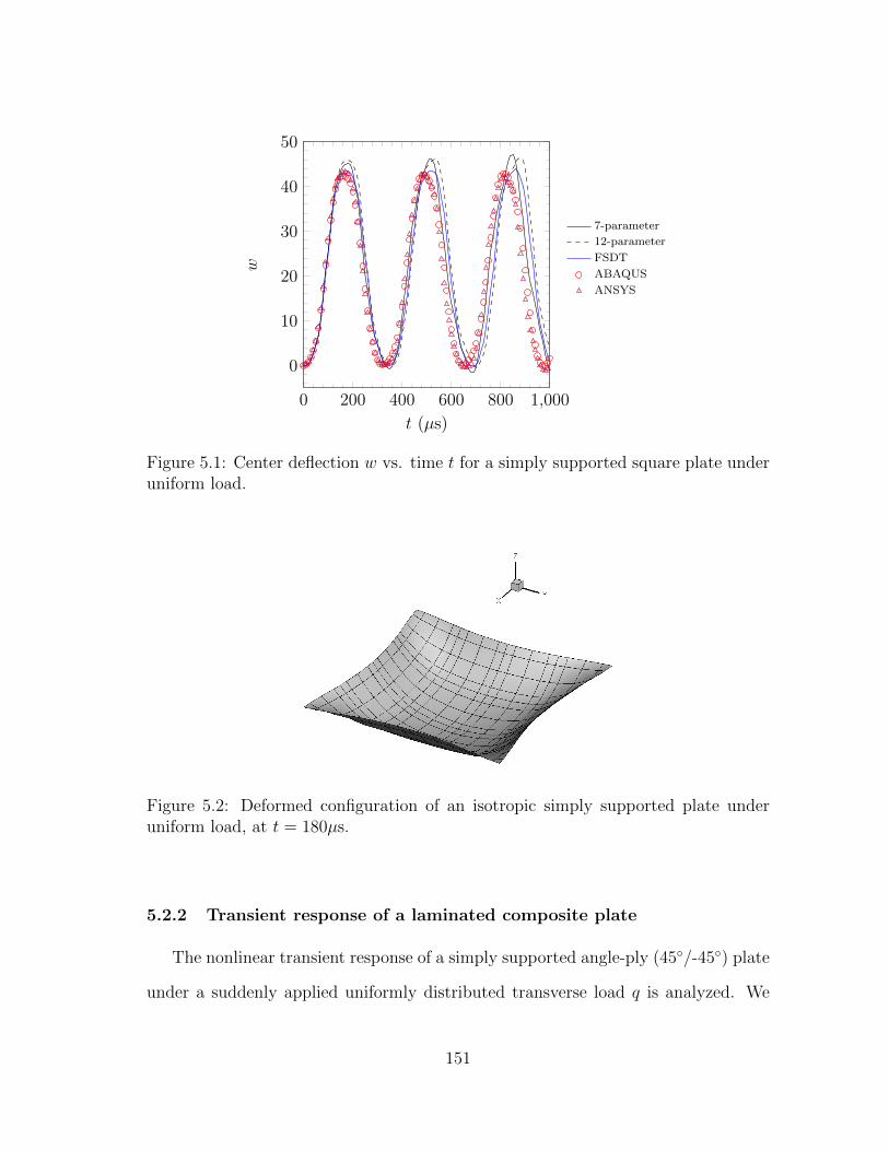
0 200 400 600 800 1,000
0
10
20
30
40
50
t (µs)
w
7-parameter
12-parameter
FSDT
ABAQUS
ANSYS
Figure 5.1: Center deflection w vs. time t for a simply supported square plate underuniform load.
Figure 5.2: Deformed configuration of an isotropic simply supported plate underuniform load, at t = 180µs.
5.2.2 Transient response of a laminated composite plate
The nonlinear transient response of a simply supported angle-ply (45/-45) plate
under a suddenly applied uniformly distributed transverse load q is analyzed. We
151

0 200 400 600 800 1,000−1
0
1
2
3
4
5
t (µs)
σxx×
105
(N/c
m2)
7-parameters
12-parameters
FSDT
ABAQUS
ANSYS
Figure 5.3: Time t vs. bending stress σxx(L/32, L/32, −h/2).
compare our results with the ones reported by Reddy [139]. The geometrical pa-
rameters are: L = 243.8 cm, h = 0.635 cm, and the load q = 50 × 10−4 N/cm2.
The material properties are assumed to be: E1 = 17.5775× 10⁶ N/cm2, E2 = E3 =
0.7031×10⁶ N/cm2, G12 = G13 = 0.35155×10⁶ N/cm2, G23 = 0.14062×10⁶ N/cm2,
ν12 = ν13 = ν23 = 0.25, and ρ = 2.547× 10⁻⁶ Ns2/cm4. The boundary conditions for
the seven-parameter formulation are
at x = 0, L uy = uz = ϕy = 0
at y = 0, L ux = uz = ϕx = 0;
while for the twelve-parameter formulation are
at x = 0, L uy = uz = ϕy = Ψy = Θy = 0
at y = 0, L ux = uz = ϕx = Ψx = Θx = 0.
152

In this case, due to the non-symmetrical layers, we model the full domain, using a
regular mesh of 4× 4, with p = 4. Figure 5.4 contains a plot of the central deflection
for the same plate, under different loads for the two formulations presented. We
observe very good agreement between the two formulations developed. Also, we
note that the period decreases, and the amplitude increases at higher loads.
0 2 4 6 8 10−0.2
0
0.2
0.4
0.6
0.8
1
1.2
1.4
Time t× 10−2 (s)
Cen
ter
defl
ecti
onuz
(cm
)
7-parameter, q
12-parameter, q
7-parameter, 2q
12-parameter, 2q
7-parameter, 3q
12-parameter, 3q
Figure 5.4: Center deflection w vs. time t for a simply supported square plate underuniform load.
Figure 5.5 shows the evolution in time of the stress in the nearest integration
point to the center of the plate. We observe very good agreement between the two
formulations, since the plate is very thin (L/h = 383.94) and there is not a big
influence of the thickness stretching.
5.2.3 Transient response of a functionally graded plate
The dynamic response for a simply supported square plate when a uniform dis-
tributed load is suddenly applied is analyzed (see Figure 4.18). The geometrical
153
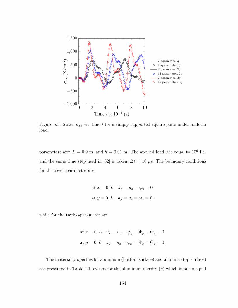
0 2 4 6 8 10−1,000
−500
0
500
1,000
1,500
Time t× 10−2 (s)
σxx
(N/c
m2) 7-parameter, q
12-parameter, q
7-parameter, 2q
12-parameter, 2q
7-parameter, 3q
12-parameter, 3q
Figure 5.5: Stress σxx vs. time t for a simply supported square plate under uniformload.
parameters are: L = 0.2 m, and h = 0.01 m. The applied load q is equal to 106 Pa,
and the same time step used in [82] is taken, ∆t = 10 µs. The boundary conditions
for the seven-parameter are
at x = 0, L ux = uz = ϕy = 0
at y = 0, L uy = uz = ϕx = 0;
while for the twelve-parameter are
at x = 0, L ux = uz = ϕy = Ψy = Θy = 0
at y = 0, L uy = uz = ϕx = Ψx = Θx = 0;
The material properties for aluminum (bottom surface) and alumina (top surface)
are presented in Table 4.1; except for the aluminum density (ρ) which is taken equal
154
to 2707 kg/m3, as in reference [82]. We take advantage of the biaxial symmetry and
model only one quadrant of the domain. We use a uniform mesh of 2×2, with p = 4.
The following non-dimensional parameters are defined
central deflection w = uz(0, 0, t)E−h/qL2
axial stress σxx = σxxh2/(qL2)
time t = t√E−/(L2ρ−).
Figure 5.6 shows the dynamic response of the aluminum-alumina plate, with
excellent agreement with the results presented in [82] (symbols). We observe that
the amplitude and the period increases, as the amount of metal in the plate also
increments. Figure 5.7 presents the dynamic response of the same plate, but this
time the ceramic surface is exposed to a temperature of 300C and the lower metallic
surface is exposed to a temperature of 20C. It is assumed that at 0C the plate is
stress free. We observe good agreement for the isotropic plates (metal and ceramic)
and a small difference for the functionally graded plates. It is seen that the initial
deflection increases, as the quantity of metal in the plate increments, in addition to
the period and amplitude as the case without thermal load.
For completeness, we also present the stresses for the cases previously discussed.
Figure 5.8 shows the evolution in time for the non-dimensional stress σxx at the top
surface in the nearest integration point to the center of the plate. Figure 5.9 shows
the same evolution, for the plate under mechanical and thermal loads, but this time
for the bottom surface that presents the highest variations. We observe that as the
content of metal increases, the plate experiences less initial compression, until it has
initial tension for the cases with n = 2 and metal. Also, there is a difference in
the initial stress between the two formulations, specially for the functionally graded
plates. This difference is attributed to the thickness stretching effect.
155

0 5 10 15 20 25−40
−30
−20
−10
0
t
w
Ceramic
n = 0.2
n = 0.5
n = 1.0
n = 2.0
Metal
Figure 5.6: Temporal evolution of center deflection of a simply supported functionallygraded plate under a suddenly applied uniform load q.
0 5 10 15 20 250
20
40
60
80
100
120
t
w
Ceramic
n = 0.2
n = 0.5
n = 1.0
n = 2.0
Metal
Figure 5.7: Temporal evolution of center deflection of a simply supported functionallygraded plate under a suddenly applied uniform load q and temperature field.
5.2.4 Transient response of an isotropic cylindrical shell
An isotropic cylindrical panel under a concentrated load P at the center and
simply supported at the two straight edges is considered (see Figure 5.10). This156

0 5 10 15 20 25−1.4
−1.2
−1
−0.8
−0.6
−0.4
−0.2
0
0.2
t
σ
Ceramic
n = 0.2
n = 0.5
n = 1.0
n = 2.0
Metal
Figure 5.8: Temporal evolution of non-dimensional stress σxx of a simply supportedfunctionally graded plate under a suddenly applied uniform load q.
0 5 10 15 20 25−2.5
−2
−1.5
−1
−0.5
0
0.5
1
t
σ
Ceramic
n = 0.2
n = 0.5
n = 1.0
n = 2.0
Metal
Figure 5.9: Temporal evolution of non-dimensional stress σxx of a simply supportedfunctionally graded plate under a suddenly applied uniform load q and temperaturefield.
157
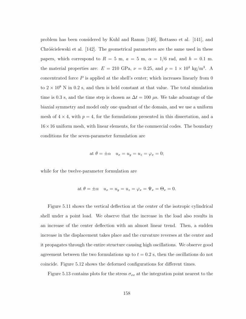
problem has been considered by Kuhl and Ramm [140], Bottasso et al. [141], and
Chroscielewski et al. [142]. The geometrical parameters are the same used in these
papers, which correspond to R = 5 m, a = 5 m, α = 1/6 rad, and h = 0.1 m.
the material properties are: E = 210 GPa, ν = 0.25, and ρ = 1 × 10⁴ kg/m3. A
concentrated force P is applied at the shell’s center; which increases linearly from 0
to 2× 10⁸ N in 0.2 s, and then is held constant at that value. The total simulation
time is 0.3 s, and the time step is chosen as ∆t = 100 µs. We take advantage of the
biaxial symmetry and model only one quadrant of the domain, and we use a uniform
mesh of 4× 4, with p = 4, for the formulations presented in this dissertation, and a
16×16 uniform mesh, with linear elements, for the commercial codes. The boundary
conditions for the seven-parameter formulation are
at θ = ±α ux = uy = uz = ϕx = 0;
while for the twelve-parameter formulation are
at θ = ±α ux = uy = uz = ϕx = Ψx = Θx = 0.
Figure 5.11 shows the vertical deflection at the center of the isotropic cylindrical
shell under a point load. We observe that the increase in the load also results in
an increase of the center deflection with an almost linear trend. Then, a sudden
increase in the displacement takes place and the curvature reverses at the center and
it propagates through the entire structure causing high oscillations. We observe good
agreement between the two formulations up to t = 0.2 s, then the oscillations do not
coincide. Figure 5.12 shows the deformed configurations for different times.
Figure 5.13 contains plots for the stress σxx at the integration point nearest to the
158
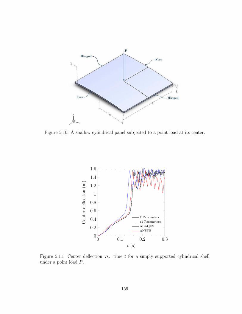
Figure 5.10: A shallow cylindrical panel subjected to a point load at its center.
0 0.1 0.2 0.30
0.2
0.4
0.6
0.8
1
1.2
1.4
1.6
t (s)
Cen
ter
defl
ecti
on(m
)
7 Parameters
12 Parameters
ABAQUS
ANSYS
Figure 5.11: Center deflection vs. time t for a simply supported cylindrical shellunder a point load P .
159
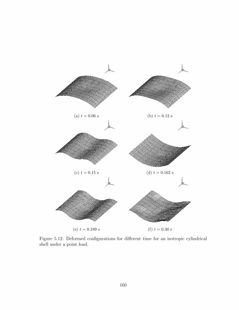
(a) t = 0.06 s (b) t = 0.12 s
(c) t = 0.15 s (d) t = 0.162 s
(e) t = 0.189 s (f) t = 0.30 s
Figure 5.12: Deformed configurations for different time for an isotropic cylindricalshell under a point load.
160
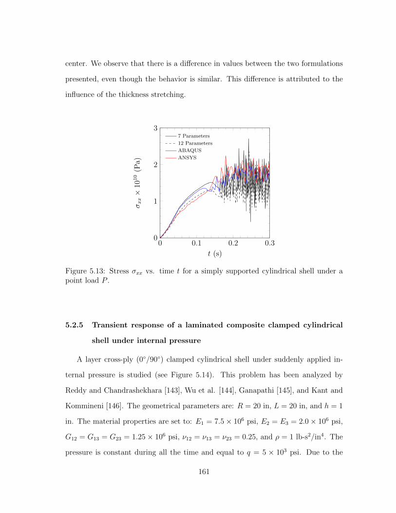
center. We observe that there is a difference in values between the two formulations
presented, even though the behavior is similar. This difference is attributed to the
influence of the thickness stretching.
0 0.1 0.2 0.30
1
2
3
t (s)
σxx×
1010
(Pa)
7 Parameters
12 Parameters
ABAQUS
ANSYS
Figure 5.13: Stress σxx vs. time t for a simply supported cylindrical shell under apoint load P .
5.2.5 Transient response of a laminated composite clamped cylindrical
shell under internal pressure
A layer cross-ply (0/90) clamped cylindrical shell under suddenly applied in-
ternal pressure is studied (see Figure 5.14). This problem has been analyzed by
Reddy and Chandrashekhara [143], Wu et al. [144], Ganapathi [145], and Kant and
Kommineni [146]. The geometrical parameters are: R = 20 in, L = 20 in, and h = 1
in. The material properties are set to: E1 = 7.5× 10⁶ psi, E2 = E3 = 2.0× 10⁶ psi,
G12 = G13 = G23 = 1.25× 10⁶ psi, ν12 = ν13 = ν23 = 0.25, and ρ = 1 lb-s2/in4. The
pressure is constant during all the time and equal to q = 5 × 10³ psi. Due to the
161

symmetry, only one octant of the domain is modeled. This problem is studied using
the presented formulations with a 2× 2 uniform mesh, with p = 4, and the commer-
cial codes ANSYS and ABAQUS with a 8 × 8 regular mesh, with linear elements.
The maximum time is t = 0.2 s and the incremental time used is the same used in
[143] ∆t = 0.001 s. The boundary conditions for the seven-parameter formulation
are
at x = 0, L ux = uy = uz = ϕx = ϕy = ϕz = Ψ = 0
while for the twelve-parameter formulation are
at x = 0, L ux = uy = uz = ϕx = ϕy = ϕz = Ψx = Ψy = Ψz = Θx = Θy = Θz = 0.
Fixed
Fixed
q A
B
C
D
Figure 5.14: Laminated composite cylinder with fixed edges subjected to internalpressure.
162
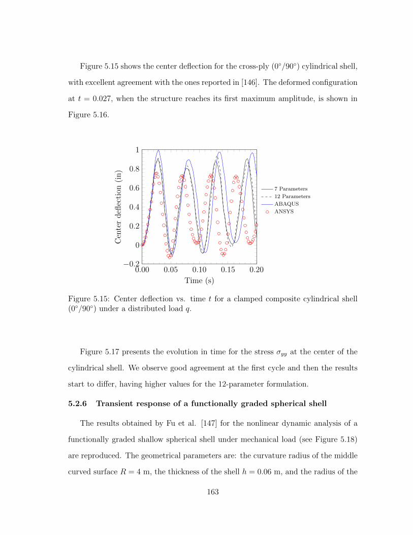
Figure 5.15 shows the center deflection for the cross-ply (0/90) cylindrical shell,
with excellent agreement with the ones reported in [146]. The deformed configuration
at t = 0.027, when the structure reaches its first maximum amplitude, is shown in
Figure 5.16.
0.00 0.05 0.10 0.15 0.20−0.2
0
0.2
0.4
0.6
0.8
1
Time (s)
Cen
ter
defl
ecti
on(i
n)
7 Parameters
12 Parameters
ABAQUS
ANSYS
Figure 5.15: Center deflection vs. time t for a clamped composite cylindrical shell(0/90) under a distributed load q.
Figure 5.17 presents the evolution in time for the stress σyy at the center of the
cylindrical shell. We observe good agreement at the first cycle and then the results
start to differ, having higher values for the 12-parameter formulation.
5.2.6 Transient response of a functionally graded spherical shell
The results obtained by Fu et al. [147] for the nonlinear dynamic analysis of a
functionally graded shallow spherical shell under mechanical load (see Figure 5.18)
are reproduced. The geometrical parameters are: the curvature radius of the middle
curved surface R = 4 m, the thickness of the shell h = 0.06 m, and the radius of the
163
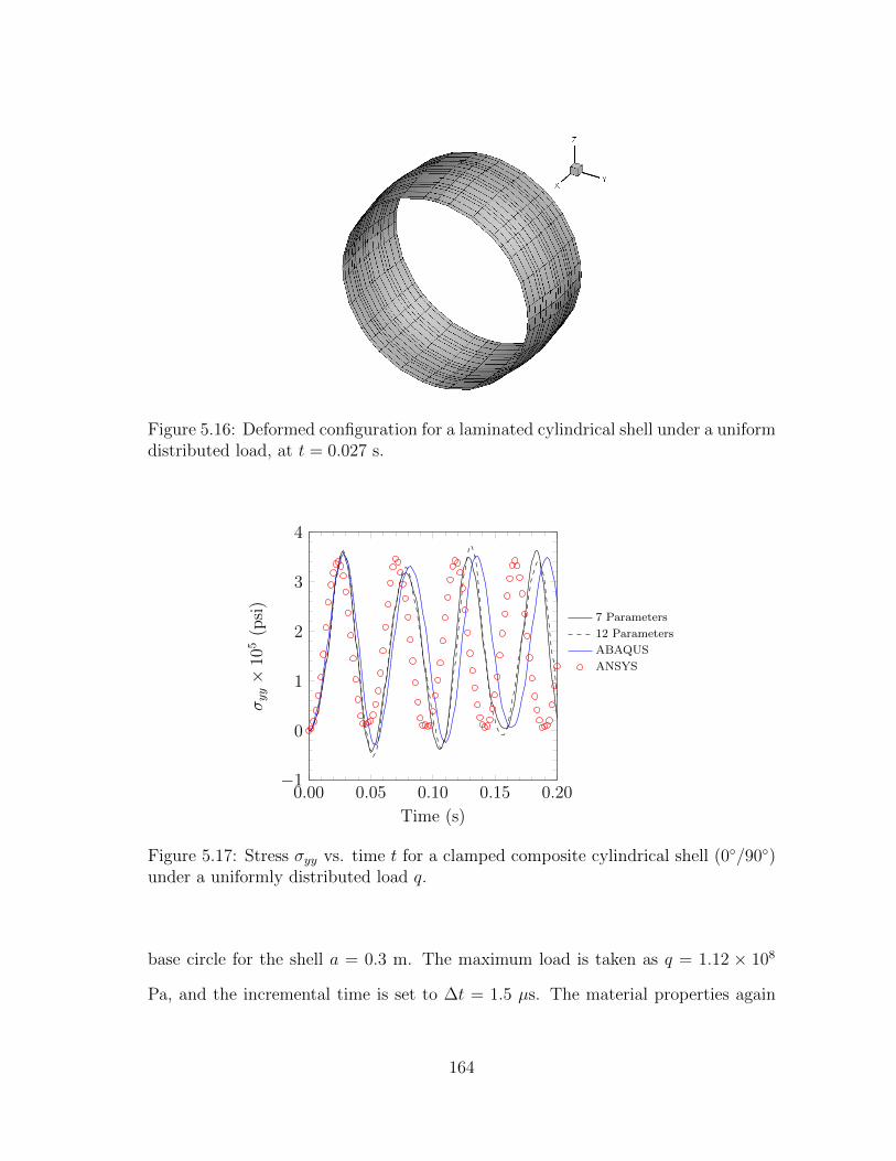
Figure 5.16: Deformed configuration for a laminated cylindrical shell under a uniformdistributed load, at t = 0.027 s.
0.00 0.05 0.10 0.15 0.20−1
0
1
2
3
4
Time (s)
σyy×
105
(psi
)
7 Parameters
12 Parameters
ABAQUS
ANSYS
Figure 5.17: Stress σyy vs. time t for a clamped composite cylindrical shell (0/90)under a uniformly distributed load q.
base circle for the shell a = 0.3 m. The maximum load is taken as q = 1.12 × 10⁸
Pa, and the incremental time is set to ∆t = 1.5 µs. The material properties again
164
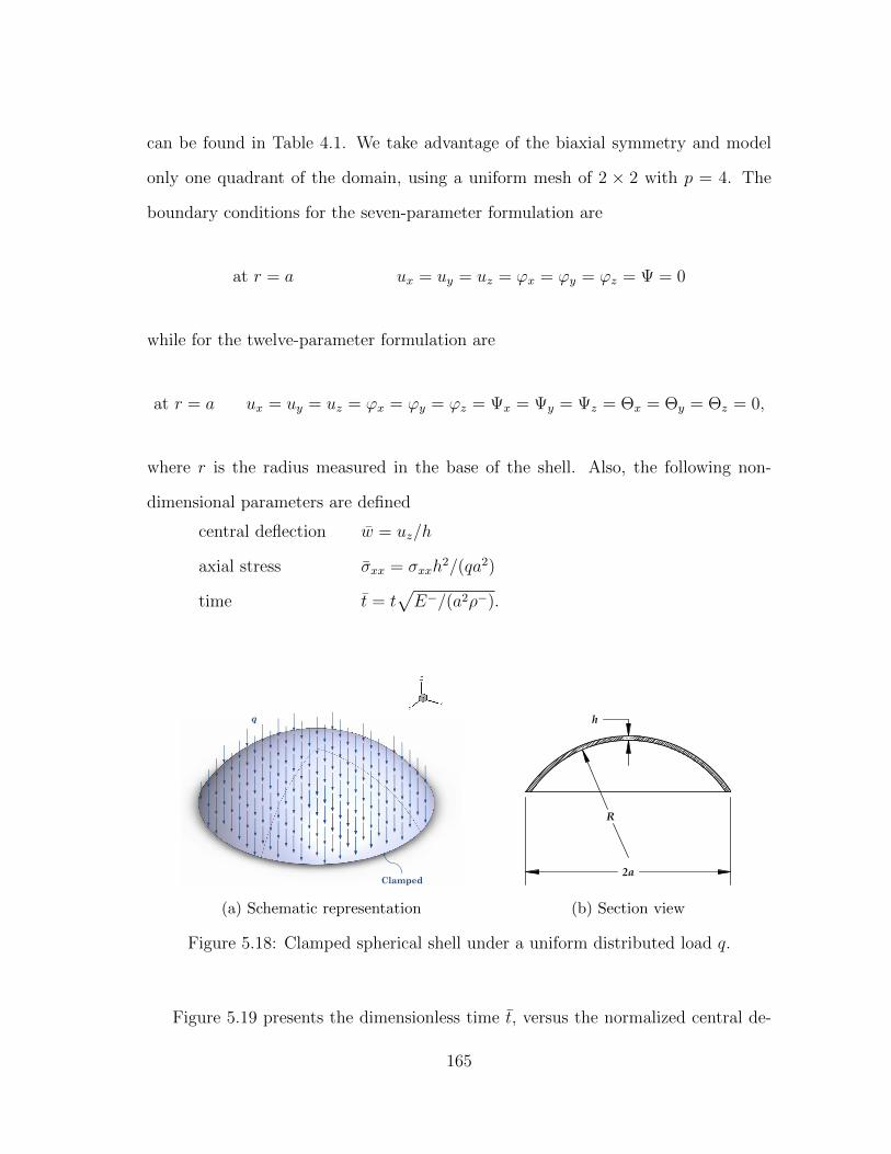
can be found in Table 4.1. We take advantage of the biaxial symmetry and model
only one quadrant of the domain, using a uniform mesh of 2 × 2 with p = 4. The
boundary conditions for the seven-parameter formulation are
at r = a ux = uy = uz = ϕx = ϕy = ϕz = Ψ = 0
while for the twelve-parameter formulation are
at r = a ux = uy = uz = ϕx = ϕy = ϕz = Ψx = Ψy = Ψz = Θx = Θy = Θz = 0,
where r is the radius measured in the base of the shell. Also, the following non-
dimensional parameters are defined
central deflection w = uz/h
axial stress σxx = σxxh2/(qa2)
time t = t√E−/(a2ρ−).
Clamped
q
(a) Schematic representation
2
DO NOT SCALE DRAWING
Part1SHEET 1 OF 1
UNLESS OTHERWISE SPECIFIED:
SCALE: 2:1 WEIGHT:
REVDWG. NO.
ASIZE
TITLE:
NAME DATE
COMMENTS:
Q.A.
MFG APPR.
ENG APPR.
CHECKED
DRAWN
FINISH
MATERIAL
3
TOLERANCING PER:INTERPRET GEOMETRIC
45
TWO PLACE DECIMAL
PROHIBITED.
THREE PLACE DECIMAL
BEND
PROPRIETARY AND CONFIDENTIAL
APPLICATION
USED ONNEXT ASSY
DIMENSIONS ARE IN INCHESTOLERANCES:FRACTIONALANGULAR: MACH
THE INFORMATION CONTAINED IN THISDRAWING IS THE SOLE PROPERTY OF<INSERT COMPANY NAME HERE>. ANY REPRODUCTION IN PART OR AS A WHOLEWITHOUT THE WRITTEN PERMISSION OF<INSERT COMPANY NAME HERE> IS
1
A
A
SECTION A-A R
h
2a
(b) Section view
Figure 5.18: Clamped spherical shell under a uniform distributed load q.
Figure 5.19 presents the dimensionless time t, versus the normalized central de-
165

flection w. We observe that the period and amplitude increase, as the metal quantity
in the shell increases. Figure 5.20 shows the deformed configuration near to the first
maximum amplitude deformation for the spherical shell with n = 2.
0 5 10 15 20 25−0.5
−0.4
−0.3
−0.2
−0.1
0
t
w
Ceramic
n = 0.5
n = 2.0
Metal
Figure 5.19: Temporal evolution of center deflection of a clamped functionally gradedshell under a suddenly applied uniform load q.
In addition to the mechanical load q = 1.0 × 10⁷ Pa, the spherical shell is also
subjected to a temperature field, 500C on the top ceramic surface and 20C on the
lower metallic surface. It is assumed that at 0C the shell is stress free. Figure 5.21
shows the evolution in time for the clamped shell under mechanical and thermal
loads. We observe that the initial deflection becomes higher, as the amount of metal
increases, in addition to a higher amplitude and period.
Figures 5.22 and 5.23 show the evolution in time for the stress σxx in the clamped
shell under mechanical and thermo-mechanical loads, respectively. The stresses are
computed at the integration point closest to the center of the spherical shell for the
166
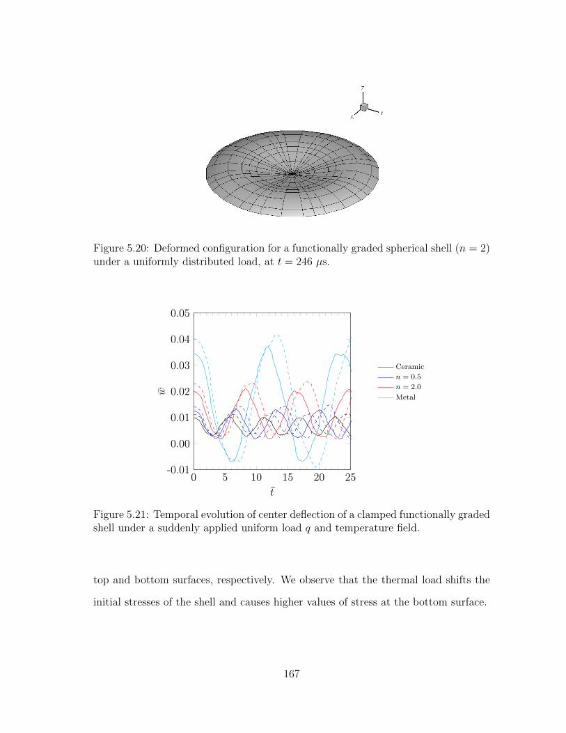
Figure 5.20: Deformed configuration for a functionally graded spherical shell (n = 2)under a uniformly distributed load, at t = 246 µs.
0 5 10 15 20 25-0.01
0.00
0.01
0.02
0.03
0.04
0.05
t
w
Ceramic
n = 0.5
n = 2.0
Metal
Figure 5.21: Temporal evolution of center deflection of a clamped functionally gradedshell under a suddenly applied uniform load q and temperature field.
top and bottom surfaces, respectively. We observe that the thermal load shifts the
initial stresses of the shell and causes higher values of stress at the bottom surface.
167

0 5 10 15 20 25−2.5
−2
−1.5
−1
−0.5
0
0.5
t
σxx
Ceramic
n = 0.5
n = 2.0
Metal
Figure 5.22: Temporal evolution of the non-dimensional stress σxx of a clampedfunctionally graded shell under a suddenly applied uniform load q.
0 5 10 15 20 25−9
−8
−7
−6
−5
−4
−3
t
σxx
Ceramic
n = 0.5
n = 2.0
Metal
Figure 5.23: Temporal evolution of the non-dimensional stress σxx of a clampedfunctionally graded shell under a suddenly applied uniform load q and temperaturefield.
168

6. CONCLUSIONS AND FUTURE RESEARCH
6.1 Summary and concluding remarks
In this dissertation, the finite element formulations, computer implementation,
and application of two different shell models, namely, the seven-parameter and
twelve-parameter shell theories, for static and transient analysis of isotropic, lam-
inated composite, and functionally graded structures have been presented. The
higher-order spectral finite element approximations of the generalized displacements
are employed to eliminate all types of locking in the shell finite elements devel-
oped herein. Transient and steady-state thermo-mechanical response of functionally
graded shells has been explored. Furthermore, in some cases, a comparison of the
results obtained with the shell elements developed herein with those obtained with
commercial codes ANSYS and ABAQUS is included.
In Chapter 2, a brief description for the equivalent single layer models based on
the higher-order shear deformation theories is presented and their advantages are
outlined. Among these we note the following: the ability of the elements to capture
the change in thickness and their respective strains and stresses, avoidance of shear
correction factors, and the inclusion of the cross-section warping, which becomes
more important when thick shells are modeled. These theories, extended to the
non-linear geometric regime, show better behavior, specially for the transient and
thermal analyses. The principal contribution in the computer implementation is the
use of static condensation of the internal nodal degrees of freedom for static and
transient analysis, which makes the finite elements more computationally efficient
and competitive with the low-order elements used in the commercial codes.
In Chapter 3, the governing equations of motion for the seven- and twelve-
169

parameter formulations are presented. A brief discussion about the strain measures
and the selection of the Green-Lagrange strain tensor is presented. The full non-linear
terms are retained in the Green–Lagrange strain tensor up to linear and quadratic
terms for the seven- and twelve-parameter formulations, respectively. The equations
for thermal strains and their linearized version used in this dissertation are included,
and details about their implementation in functionally graded shells are presented.
In the subsequent two chapters computer implementation of the finite element
models of the equations of motion is discussed. In Chapter 4, we present the two
methods of solution for static analysis (Newton’s and arc length) and apply those to
the two formulations discussed. Several examples to show the capability of the ele-
ments by comparing the numerical results with each other and with those obtained
using the commercial codes ANSYS and ABAQUS are given. The first two examples,
show the ability for the present formulations to reproduce the change in thickness
predicted analytically for isotropic shells, revealing that the twelve-parameter ele-
ment is more accurate, specially near the edges. The next two examples illustrate
good agreement between these formulations and experimental results for laminated
composite plates. The fifth example shows a good agreement between the seven- and
twelve-parameter formulations presented and the analytical solution for functionally
graded plates, and it also shows how those elements perform better for the stress
prediction when the change in temperature between the top and bottom surfaces is
high. The rest of the examples included are several benchmark problems available
in the literature, which are reproduced using the presented formulations to show
their ability to accurately describe the response. We find that the seven-parameter
formulation is stiffer when compared with the twelve-parameter formulation. The
displacements and stresses are slightly lower for the seven-parameter formulation.
Also, we observe better behavior of the twelve-parameter formulation for finite rota-
170
tions when Poisson’s ratio is different from zero. Furthermore, the two formulations
presented produce close stress values to the ones obtained by means of three dimen-
sional finite elements in the commercial codes, using considerably less computational
resources.
In Chapter 5, the finite element model to solve time dependent problems using
Newmark’s scheme is presented. Several examples are solved to show the performance
of the presented formulations. First, three comparisons for the results obtained by
means of the present elements with solutions found in the literature using the first-
order shear deformation theory (FSDT) for plates, made of different materials, are
presented. We observe that the behavior of the twelve-parameter formulation is sig-
nificantly better for thick plates (or shells in our model), showing better conservation
of the period and amplitude, being the latter also higher than the one found using
the FSDT. In the next example we explored the snap-throw behavior for an isotropic
cylindrical shell. We observe good agreement in the initial behavior and then the os-
cillations show some differences. The stress behavior is found to be different. Then,
the transient response of a cylindrical composite shell is analyzed with excellent
agreement. Finally, the transient response for a thick functionally graded spheri-
cal shell is studied. It is found that there is a slight difference in the amplitudes
and periods between the responses predicted by the seven- and twelve-parameter
formulations.
6.2 Future research
There are some areas that need further investigation in order to make the present
study more complete. The following tasks are suggested for future works:
a) Nonlinear material models. Since the shell undergoes large deformations, it
is possible that the shell goes beyond the elastic limit. Hence, the current
171

elements should be extended to account for inelastic material behavior.
b) Since stress distributions in a structure can exceed the allowable limit, damage
may develop in the structure. In particular, for laminated composites the
interlaminar stresses can result in delamination. In addition, other types of
damage like matrix cracking, fiber breakage, or partial delamination could be
developed. Incorporating damage models into the elements developed herein
would be a very useful and practical study.
c) In this study linear or quadratic terms of strains are included. Higher-order
components of the strain may be included to understand their contribution to
the overall response of structures undergoing large deformations. It has been
shown that higher-order components of strain improve the transient response.
Thus, this is another possible extension of the present elements.
d) The formulations presented herein may be extended to account actuating and
sensing layers (e.g., piezoelectric materials) in composite structures.
e) In the case of fiber-reinforced composite structures, there can be a change in
the fiber angle from its undeformed value as the body deforms. Extending the
present formulation to account for the change in the lamination angles as a
function of deformation is of practical interest.
f) One may also investigate the effect of higher-order time integration algorithms
on the transient response. The presence of spurious oscillations in the transient
analysis can be filtered using higher-order time integration algorithms.
g) The elements presented here are able to reproduce large deformation accu-
rately. However, the main disadvantaged at this time is the mesh generation
172

for complex structures. For this reason, it is recommended to create an efficient
software that can be used to generate the mesh for complicated shapes.
173

REFERENCES
[1] D. Chapelle and K.-J. Bathe, The finite element analysis of shells-
fundamentals. Springer, 2003.
[2] J. N. Reddy, Theory and Analysis of Elastic Plates and Shells, second. ed.
Philadelphia, PA: Taylor & Francis, 2007.
[3] R. A. Arciniega, “On a tensor-based finite element model for the analysis of
shell structures,” Ph.D. dissertation, Texas A&M University, College Station,
Texas, 2005.
[4] J. N. Reddy, Mechanics of laminated composite plates and shells: theory and
analysis. CRC press, 2004.
[5] M. Amabili, Nonlinear vibrations and stability of shells and plates. Cambridge
University Press, 2008.
[6] E. Reissner, “On transverse bending of plates, including the effect of transverse
shear deformation,” International Journal of Solids and Structures, vol. 11,
no. 5, pp. 569–573, 1975.
[7] K. Lo, R. Christensen, and E. Wu, “A high-order theory of plate deformation
- Part 1: Homogeneous plates,” Journal of Applied Mechanics, vol. 44, no. 4,
pp. 663–668, 1977.
[8] ——, “A high-order theory of plate deformation - Part 2: laminated plates,”
Journal of Applied Mechanics, vol. 44, no. 4, pp. 669–676, 1977.
[9] K.-J. Bathe, Finite element procedures. Prentice-Hall, 1996.
[10] G. S. Payette, “Spectral/hp finite element models for fluids and structures,”
Ph.D. dissertation, Texas A&M University, College Station, Texas, 2012.
174

[11] H.-C. Huang, Static and Dynamic Analysis of Plates and Shells. Springer,
London, 1989.
[12] S. Ahmad, B. M. Irons, and O. Zienkiewicz, “Analysis of thick and thin shell
structures by curved finite elements,” International Journal for Numerical
Methods in Engineering, vol. 2, no. 3, pp. 419–451, 1970.
[13] P. Wriggers, Nonlinear finite element methods. Springer Science & Business
Media, 2008.
[14] O. Zienkiewicz, R. Taylor, and J. Too, “Reduced integration technique in gen-
eral analysis of plates and shells,” International Journal for Numerical Methods
in Engineering, vol. 3, no. 2, pp. 275–290, 1971.
[15] H. Stolarski and T. Belytschko, “Membrane locking and reduced integration
for curved elements,” Journal of Applied Mechanics, vol. 49, no. 1, pp. 172–176,
1982.
[16] W. Altman and F. Iguti, “A thin cylindrical shell finite element based on a
mixed formulation,” Computers & Structures, vol. 6, no. 2, pp. 149–155, 1976.
[17] T. Belytschko and I. Leviathan, “Physical stabilization of the 4-node shell
element with one point quadrature,” Computer Methods in Applied Mechanics
and Engineering, vol. 113, no. 3, pp. 321–350, 1994.
[18] E. N. Dvorkin and K.-J. Bathe, “A continuum mechanics based four-node shell
element for general non-linear analysis,” Engineering Computations, vol. 1,
no. 1, pp. 77–88, 1984.
[19] E. Hinton and H. Huang, “A family of quadrilateral mindlin plate elements
with substitute shear strain fields,” Computers & Structures, vol. 23, no. 3, pp.
409–431, 1986.
175
[20] J. Simo and M. Rifai, “A class of mixed assumed strain methods and the
method of incompatible modes,” International Journal for Numerical Methods
in Engineering, vol. 29, no. 8, pp. 1595 – 1638, 1990.
[21] I. Babuska, B. A. Szabo, and I. N. Katz, “The p-version of the finite element
method,” SIAM Journal on Numerical Analysis, vol. 18, no. 3, pp. 515–545,
1981.
[22] R. Arciniega and J. N. Reddy, “Tensor-based finite element formulation for geo-
metrically nonlinear analysis of shell structures,” Computer Methods in Applied
Mechanics and Engineering, vol. 196, no. 4 – 6, pp. 1048 – 1073, 2007.
[23] ——, “Large deformation analysis of functionally graded shells,” Int. J. Solids
Struct., vol. 44, no. 6, pp. 2036 – 2052, 2007.
[24] G. Payette and J. Reddy, “A seven-parameter spectral/hp finite element formu-
lation for isotropic, laminated composite and functionally graded shell struc-
tures,” Comput. Methods Appl. Mech. Eng., vol. 278, pp. 664 – 704, 2014.
[25] M. Amabili, “A non-linear higher-order thickness stretching and shear deforma-
tion theory for large-amplitude vibrations of laminated doubly curved shells,”
International Journal of Non-linear Mechanics, vol. 58, pp. 57 – 75, 2014.
[26] ——, “Non-linearities in rotation and thickness deformation in a new third-
order thickness deformation theory for static and dynamic analysis of isotropic
and laminated doubly curved shells,” International Journal of Non-linear Me-
chanics, vol. 69, pp. 109 – 128, 2015.
[27] M. Gutierrez Rivera and J. N. Reddy, “Stress analysis of func-
tionally graded shells using a 7-parameter shell element,” Me-
176

chanics Research Communications, pp. –, 2016. [Online]. Available:
http://www.sciencedirect.com/science/article/pii/S0093641316000343
[28] M. Gutierrez Rivera, J. N. Reddy, and M. Amabili, “A new twelve-parameter
spectral/hp shell finite element for large deformation analysis of composite
shells,” Composite Structures, vol. 151, pp. 183–196, 2016.
[29] A. Love, The mathematical theory of elasticity, 1927.
[30] R. D. Mindlin, “Influence of rotatory inertia and shear on flexural motions
of isotropic, elastic plates,” Journal of Applied Mechanics, vol. 18, no. 1, pp.
31–39, 1951.
[31] G. Kirchhoff, “Uber das gleichgewicht und die bewegung einer elastischen
scheibe.” Journal fur die reine und angewandte Mathematik, vol. 40, pp.
51–88, 1850. [Online]. Available: http://eudml.org/doc/147439
[32] H.-T. Thai and S.-E. Kim, “A review of theories for the modeling and analysis
of functionally graded plates and shells,” Composite Structures, vol. 128, pp.
70–86, 2015.
[33] O. C. Zienkiewicz and R. L. Taylor, The finite element method. London:
McGraw-Hill, 1977.
[34] E. Reissner, “The effect of transverse shear deformation on the bending of
elastic plates,” Journal of Applied Mechanics, vol. 12, no. 2, pp. 69–77, 1945.
[35] C. Wang, G. Lim, J. Reddy, and K. Lee, “Relationships between bending so-
lutions of reissner and mindlin plate theories,” Engineering Structures, vol. 23,
no. 7, pp. 838–849, 2001.
[36] J. N. Reddy, An Introduction Nonlinear Finite Element Analysis, 2nd ed. Ox-
ford, UK: Oxford University Press, 2015.
177
[37] V. Novozhilov, The theory of thin shells. P. Noordhoff, 1959.
[38] B. Bassa, F. Sabourin, and M. Brunet, “A new nine-node solid-shell finite
element using complete 3d constitutive laws,” International Journal for Nu-
merical Methods in Engineering, vol. 92, no. 7, pp. 589–636, 2012.
[39] A. K. Garg, R. K. Khare, and T. Kant, “Higher-order closed-form solutions
for free vibration of laminated composite and sandwich shells,” Journal of
Sandwich Structures and Materials, vol. 8, no. 3, pp. 205–235, 2006.
[40] T. Kant, “Numerical analysis of thick plates,” Computer Methods in Applied
Mechanics and Engineering, vol. 31, no. 1, pp. 1–18, 1982.
[41] T. Kant, D. Owen, and O. Zienkiewicz, “A refined higher-order C0 plate bend-
ing element,” Computers & Structures, vol. 15, no. 2, pp. 177–183, 1982.
[42] J. N. Reddy, “A refined nonlinear theory of plates with transverse shear de-
formation,” International Journal of Solids and Structures, vol. 20, no. 9, pp.
881–896, 1984.
[43] ——, “A simple higher-order theory for laminated composite plates,” Journal
of Applied Mechanics, vol. 51, no. 4, pp. 745–752, 1984.
[44] J. Reddy and C. Liu, “A higher-order shear deformation theory of laminated
elastic shells,” International Journal of Engineering Science, vol. 23, no. 3, pp.
319–330, 1985.
[45] R. A. Arciniega and J. Reddy, “Consistent third-order shell theory with appli-
cation to composite cylindrical cylinders,” AIAA Journal, vol. 43, no. 9, pp.
2024–2038, 2005.
178
[46] T. Kant and B. Manjunatha, “An unsymmetric frc laminate C0 finite element
model with 12 degrees of freedom per node,” Engineering Computations, vol. 5,
no. 4, pp. 300–308, 1988.
[47] S. Khalili, S. Tafazoli, and K. M. Fard, “Free vibrations of laminated composite
shells with uniformly distributed attached mass using higher order shell theory
including stiffness effect,” Journal of Sound and Vibration, vol. 330, no. 26,
pp. 6355–6371, 2011.
[48] S. Khalili, A. Davar, and K. M. Fard, “Free vibration analysis of homogeneous
isotropic circular cylindrical shells based on a new three-dimensional refined
higher-order theory,” International Journal of Mechanical Sciences, vol. 56,
no. 1, pp. 1–25, 2012.
[49] A. Davar, S. Khalili, and K. M. Fard, “Assessment of different higher order the-
ories for low-velocity impact analysis of fibre-metal laminate cylindrical shells,”
Proceedings of the Institution of Mechanical Engineers, Part L: Journal of Ma-
terials Design and Applications, vol. 228, no. 3, pp. 160–189, 2014.
[50] N. Buchter, E. Ramm, and D. Roehl, “Three-dimensional extension of non-
linear shell formulation based on the enhanced assumed strain concept,” In-
ternational Journal for Numerical Methods in Engineering, vol. 37, no. 15, pp.
2551 – 2568, 1994.
[51] M. Bischoff and E. Ramm, “Shear deformable shell elements for large strains
and rotations,” International Journal for Numerical Methods in Engineering,
vol. 40, no. 23, pp. 4427 – 4449, 1997.
[52] ——, “On the physical significance of higher order kinematic and static vari-
ables in a three-dimensional shell formulation,” International Journal of Solids
and Structures, vol. 37, no. 46 – 47, pp. 6933 – 6960, 2000.
179
[53] H. Parisch, “A continuum-based shell theory for non-linear applications,” In-
ternational Journal for Numerical Methods in Engineering, vol. 38, no. 11, pp.
1855 – 1883, 1995.
[54] C. Sansour, “A theory and finite element formulation of shells at finite deforma-
tions involving thickness change: circumventing the use of a rotation tensor,”
Archive of Applied Mechanics, vol. 65, no. 3, pp. 194 – 216, 1995.
[55] M. Amabili and J. N. Reddy, “A new non-linear higher-order shear deforma-
tion theory for large-amplitude vibrations of laminated doubly curved shells,”
International Journal of Non-linear Mechanics, vol. 45, no. 4, pp. 409 – 418,
2010.
[56] E. Carrera, “A study of transverse normal stress effect on vibration of multi-
layered plates and shells,” Journal of Sound and Vibration, vol. 225, no. 5, pp.
803–829, 1999.
[57] M. Amabili, “Nonlinear vibrations of laminated circular cylindrical shells: com-
parison of different shell theories,” Composite Structures, vol. 94, no. 1, pp.
207–220, 2011.
[58] F. Alijani and M. Amabili, “Nonlinear vibrations of thick laminated circular
cylindrical panels,” Composite Structures, vol. 96, pp. 643–660, 2013.
[59] M. Amabili, “A new nonlinear higher-order shear deformation theory with
thickness variation for large-amplitude vibrations of laminated doubly curved
shells,” Journal of Sound and Vibration, vol. 332, no. 19, pp. 4620 – 4640,
2013.
[60] V. Vallala, “Higher-order spectral/hp finite element technology for sturctures
and fluid flows,” Ph.D. dissertation, Texas A&M University, College Station,
180

Texas, 2013.
[61] J. N. Reddy and R. Arciniega, “Shear deformation plate and shell theories:
from stavsky to present,” Mechanics of Advanced Materials and Structures,
vol. 11, no. 6, pp. 535–582, 2004.
[62] U. Heisserer, S. Hartmann, A. Duster, and Z. Yosibash, “On volumetric
locking-free behaviour of p-version finite elements under finite deformations,”
Communications in Numerical Methods in Engineering, vol. 24, no. 11, pp.
1019–1032, 2008.
[63] N. Kim and J. N. Reddy, “A spectral/hp least-squares finite element analysis
of the carreau–yasuda fluids,” International Journal for Numerical Methods in
Fluids, 2016.
[64] D. Gottlieb and S. A. Orszag, Numerical analysis of spectral methods: theory
and applications. Siam, 1977, vol. 26.
[65] J. Pontaza and J. Reddy, “Spectral/hp least-squares finite element formulation
for the navier–stokes equations,” Journal of Computational Physics, vol. 190,
no. 2, pp. 523–549, 2003.
[66] ——, “Space–time coupled spectral/hp least-squares finite element formula-
tion for the incompressible navier–stokes equations,” Journal of Computational
Physics, vol. 197, no. 2, pp. 418–459, 2004.
[67] G. Payette and J. Reddy, “On the roles of minimization and linearization
in least-squares finite element models of nonlinear boundary-value problems,”
Journal of Computational Physics, vol. 230, no. 9, pp. 3589–3613, 2011.
[68] A. Zak and M. Krawczuk, “Static and dynamic analysis of isotropic shell struc-
tures by the spectral finite element method,” in Journal of Physics: Conference
181

Series, vol. 382, no. 1. IOP Publishing, 2012, p. 012054.
[69] G. Karniadakis and S. Sherwin, Spectral/hp Element Methods for CFD, 1st ed.
Oxford: Oxford University Press, 1999.
[70] J. N. Reddy, Applied functional analysis and variational methods in engineer-
ing. Mcgraw-Hill College, 1986.
[71] P. B. Galvin, G. Gagne, and A. Silberschatz, Operating system concepts. John
Wiley & Sons, Inc., 2013.
[72] P. Naghdi, “Theory of shells and plates,” S. Flgge, C. Truesdell (Eds.), Hand-
buch der Physik, vol. VIa/2, pp. 425 – 640, 1972.
[73] O. Starkova and A. Aniskevich, “Poisson’s ratio and the incompressibility re-
lation for various strain measures with the example of a silica-filled sbr rubber
in uniaxial tension tests,” Polymer Testing, vol. 29, no. 3, pp. 310–318, 2010.
[74] C. Truesdell, The mechanical foundations of elasticity and fluid dynamics.
Gordon & Breach Science Pub, 1966, vol. 8.
[75] J. N. Reddy, An Introduction to Continuum Mechanics, 2nd ed. New York:
Cambridge University Press, 2013.
[76] Y. Basar and D. Weichert, Nonlinear Continuum Mechanics of Solids: Fun-
damental Mathematical and Physical Concepts. Springer Science & Business
Media, 2000.
[77] R. Stojanovitch, S. Djuritch, and L. Vujoshevitch, “On finite thermal defor-
mations,” Archiwum Mechaniki Stosowanej, vol. 16, pp. 103–108, 1964.
[78] L. Vujosevic and V. Lubarda, “Finite-strain thermoelasticity based on mul-
tiplicative decomposition of deformation gradient,” Theoretical and Applied
Mechanics, vol. 28, no. 29, pp. 379–399, 2002.
182
[79] M. H. Sadd, Elasticity: theory, applications, and numerics. Academic Press,
2009.
[80] M. Yamanouchi and M. Koizumi, “Functionally gradient materials.” Pro-
ceeding of the first international symposium on functionally graded materials,
1991.
[81] M. Koizumi, “The concept of fgm,” 1993.
[82] G. Praveen and J. Reddy, “Nonlinear transient thermoelastic analysis of func-
tionally graded ceramic-metal plates,” International Journal of Solids and
Structures, vol. 35, no. 33, pp. 4457 – 4476, 1998.
[83] R. Javaheri and M. Eslami, “Thermal buckling of functionally graded plates,”
AIAA Journal, vol. 40, no. 1, pp. 162–169, 2002.
[84] H.-S. Shen, Functionally graded materials: nonlinear analysis of plates and
shells. Taylor & Francis, 2009.
[85] J. N. Reddy, Energy principles and variational methods in applied mechanics,
2nd ed. New York: John Wiley & Sons, 2002.
[86] J. Bonet and R. D. Wood, Nonlinear continuum mechanics for finite element
analysis. Cambridge university press, 1997.
[87] E. Riks, “An incremental approach to the solution of snapping and buckling
problems,” International Journal of Solids and Structures, vol. 15, no. 7, pp.
529–551, 1979.
[88] ——, “Some computational aspects of the stability analysis of nonlinear struc-
tures,” Computer Methods in Applied Mechanics and Engineering, vol. 47,
no. 3, pp. 219–259, 1984.
183

[89] M. A. Crisfield, “A fast incremental/iterative solution procedure that handles
snap-through,” Computers & Structures, vol. 13, no. 1, pp. 55–62, 1981.
[90] J. Kweon and C. Hong, “An improved arc-length method for postbuckling
analysis of composite cylindrical panels,” Computers & structures, vol. 53,
no. 3, pp. 541–549, 1994.
[91] ABAQUS, Analysis User’s Manual, version 6.12 ed., Dassault Systemes, USA,
2012.
[92] ANSYS, Help System, Element library, release 12.1 ed., ANSYS, Inc., USA,
2009.
[93] E. J. Barbero, Finite element analysis of composite materials using AbaqusTM.
CRC press, 2013.
[94] F. Alijani and M. Amabili, “Non-linear static bending and forced vibrations of
rectangular plates retaining non-linearities in rotations and thickness deforma-
tion,” International Journal of Non-linear Mechanics, vol. 67, pp. 394 – 404,
2014.
[95] S. Zaghloul and J. Kennedy, “Nonlinear behavior of symmetrically laminated
plates,” Journal of Applied Mechanics, vol. 42, no. 1, pp. 234–236, 1975.
[96] N. Putcha and J. Reddy, “A refined mixed shear flexible finite element for the
nonlinear analysis of laminated plates,” Computers & Structures, vol. 22, no. 4,
pp. 529–538, 1986.
[97] J. H. Starnes Jr and M. Rouse, “Postbuckling and failure characteristics of
selected flat rectangular graphite-epoxy plates loaded in compression,” AIAA
Paper, vol. 81, no. 0543, pp. 423–434, 1981.
184
[98] S. Engelstad, J. Eddy, and N. Night, “Postbuckling response and failure predic-
tion of graphite-epoxy plates loaded in compression,” AIAA Journal, vol. 30,
no. 8, pp. 2106–2113, 1992.
[99] J. Woo and S. Meguid, “Nonlinear analysis of functionally graded plates and
shallow shells,” International Journal of Solids and Structures, vol. 38, no. 42,
pp. 7409–7421, 2001.
[100] G. Horrigmoe and P. G. Bergan, “Nonlinear analysis of free-form shells by flat
finite elements,” Computer Methods in Applied Mechanics and Engineering,
vol. 16, no. 1, pp. 11–35, 1978.
[101] J. Simo, M. Rifai, and D. Fox, “On a stress resultant geometrically exact shell
model. part iv: Variable thickness shells with through-the-thickness stretch-
ing,” Computer Methods in Applied Mechanics and Engineering, vol. 81, no. 1,
pp. 91–126, 1990.
[102] H. C. Park, C. Cho, and S. W. Lee, “An efficient assumed strain element model
with six dof per node for geometrically non-linear shells,” International Journal
for Numerical Methods in Engineering, vol. 38, no. 24, pp. 4101–4122, 1995.
[103] P. Betsch, F. Gruttmann, and E. Stein, “A 4-node finite shell element for the
implementation of general hyperelastic 3d-elasticity at finite strains,” Com-
puter Methods in Applied Mechanics and Engineering, vol. 130, no. 1, pp. 57–
79, 1996.
[104] N. El-Abbasi and S. Meguid, “A new shell element accounting for through-
thickness deformation,” Computer Methods in Applied Mechanics and Engi-
neering, vol. 189, no. 3, pp. 841–862, 2000.
185
[105] K. Sze, X. Liu, and S. Lo, “Popular benchmark problems for geometric nonlin-
ear analysis of shells,” Finite Elements in Analysis and Design, vol. 40, no. 11,
pp. 1551 – 1569, 2004.
[106] K.-M. Hsiao and Y.-R. Chen, “Nonlinear analysis of shell structures by degen-
erated isoparametric shell element,” Computers & Structures, vol. 31, no. 3,
pp. 427–438, 1989.
[107] J. C. Simo, D. D. Fox, and M. S. Rifai, “On a stress resultant geometrically
exact shell model. part iii: Computational aspects of the nonlinear theory,”
Computer Methods in Applied Mechanics and Engineering, vol. 79, no. 1, pp.
21–70, 1990.
[108] J. Chroscielewski, J. Makowski, and H. Stumpf, “Genuinely resultant shell
finite elements accounting for geometric and material non-linearity,” Interna-
tional Journal for Numerical Methods in Engineering, vol. 35, no. 1, pp. 63–94,
1992.
[109] F. Flores, E. Onate, and F. Zarate, “New assumed strain triangles for non
linear shell analysis,” Computational Mechanics, vol. 17, no. 1-2, pp. 107–114,
1995.
[110] P. Betsch, A. Menzel, and E. Stein, “On the parametrization of finite rotations
in computational mechanics: A classification of concepts with application to
smooth shells,” Computer Methods in Applied Mechanics and Engineering, vol.
155, no. 3, pp. 273–305, 1998.
[111] P. Mohan and R. Kapania, “Updated lagrangian formulation of a flat triangular
element for thin laminated shells,” AIAA Journal, vol. 36, no. 2, pp. 273–281,
1998.
186
[112] W. I. Hong, J. H. Kim, Y. H. Kim, and S. W. Lee, “An assumed strain tri-
angular curved solid shell element formulation for analysis of plates and shells
undergoing finite rotations,” International Journal for Numerical Methods in
Engineering, vol. 52, no. 7, pp. 747–761, 2001.
[113] S. Levyakov and V. Kuznetsov, “Application of triangular element invariants
for geometrically nonlinear analysis of functionally graded shells,” Computa-
tional Mechanics, vol. 48, no. 4, pp. 499–513, 2011.
[114] H. Parisch, “An investigation of a finite rotation four node assumed strain
shell element,” International Journal for Numerical Methods in Engineering,
vol. 31, no. 1, pp. 127–150, 1991.
[115] P. Massin and M. A. Mikdad, “Nine node and seven node thick shell elements
with large displacements and rotations,” Computers & Structures, vol. 80, no.
9 – 10, pp. 835 – 847, 2002.
[116] S. Timoshenko and J. Gere, Theory of Elastic Stability, 2nd ed. New York:
Dover Publications, 1989.
[117] MatWeb, LLC. Online Materials Information Resource - MatWeb. Accessed
June 23 2016. [Online]. Available: http://www.matweb.com/
[118] N. Buechter and E. Ramm, “Shell theory versus degenerationa comparison
in large rotation finite element analysis,” International Journal for Numerical
Methods in Engineering, vol. 34, no. 1, pp. 39–59, 1992.
[119] B. Brank, D. Peric, and F. Damjanic, “On implementation of a nonlinear four
node shell finite element for thin multilayered elastic shells,” Computational
Mechanics, vol. 16, no. 5, pp. 341–359, 1995.
187
[120] C. Sansour and J. Bocko, “On hybrid stress, hybrid strain and enhanced strain
finite element formulations for a geometrically exact shell theory with drilling
degrees of freedom,” International Journal for Numerical Methods in Engineer-
ing, vol. 43, no. 1, pp. 175–192, 1998.
[121] C. Sansour and F. Kollmann, “Families of 4-node and 9-node finite elements for
a finite deformation shell theory. an assesment of hybrid stress, hybrid strain
and enhanced strain elements,” Computational Mechanics, vol. 24, no. 6, pp.
435–447, 2000.
[122] A. Beheshti and S. Ramezani, “Nonlinear finite element analysis of function-
ally graded structures by enhanced assumed strain shell elements,” Applied
Mathematical Modelling, vol. 39, no. 13, pp. 3690–3703, 2015.
[123] J. M. Gere and S. P. Timoshenko, Mechanics of materials, second ed. ed.
California: PWS Publishers, 1989.
[124] O. O. Ochoa and J. N. Reddy, Finite element analysis of composite laminates.
Springer, 1992.
[125] F. Gruttmann, E. Stein, and P. Wriggers, “Theory and numerics of thin elastic
shells with finite rotations,” Ingenieur-Archiv, vol. 59, no. 1, pp. 54–67, 1989.
[126] C. Sansour and H. Bufler, “An exact finite rotation shell theory, its mixed
variational formulation and its finite element implementation,” International
Journal for Numerical Methods in Engineering, vol. 34, no. 1, pp. 73–115, 1992.
[127] L. Jiang and M. Chernuka, “A simple four-noded corotational shell element
for arbitrarily large rotations,” Computers & Structures, vol. 53, no. 5, pp.
1123–1132, 1994.
188

[128] N. Stander, A. Matzenmiller, and E. Ramm, “An assessment of assumed strain
methods in finite rotation shell analysis,” Engineering Computations, vol. 6,
no. 1, pp. 58–66, 1989.
[129] S. Klinkel, F. Gruttmann, and W. Wagner, “A continuum based three-
dimensional shell element for laminated structures,” Computers & Structures,
vol. 71, no. 1, pp. 43–62, 1999.
[130] R. H. Macneal and R. L. Harder, “A proposed standard set of problems to test
finite element accuracy,” Finite elements in Analysis and Design, vol. 1, no. 1,
pp. 3–20, 1985.
[131] Y. Basar and Y. Ding, “Finite-rotation shell elements for the analysis of finite-
rotation shell problems,” International Journal for Numerical Methods in En-
gineering, vol. 34, no. 1, pp. 165–169, 1992.
[132] R. Hauptmann and K. Schweizerhof, “A systematic development of solid-
shellelement formulations for linear and non-linear analyses employing only
displacement degrees of freedom,” International Journal for Numerical Meth-
ods in Engineering, vol. 42, no. 1, pp. 49–69, 1998.
[133] E. Providas and M. Kattis, “A simple finite element model for the geometrically
nonlinear analysis of thin shells,” Computational Mechanics, vol. 24, no. 2, pp.
127–137, 1999.
[134] Y. Basar, Y. Ding, and R. Schultz, “Refined shear-deformation models for
composite laminates with finite rotations,” International Journal of Solids and
Structures, vol. 30, no. 19, pp. 2611–2638, 1993.
[135] W. Wagner and F. Gruttmann, “A simple finite rotation formulation for com-
posite shell elements,” Engineering Computations, vol. 11, no. 2, pp. 145–176,
189

1994.
[136] Y. Basar, M. Itskov, and A. Eckstein, “Composite laminates: nonlinear inter-
laminar stress analysis by multi-layer shell elements,” Computer Methods in
Applied Mechanics and Engineering, vol. 185, no. 2, pp. 367–397, 2000.
[137] M. Balah and H. N. Al-Ghamedy, “Finite element formulation of a third or-
der laminated finite rotation shell element,” Computers & Structures, vol. 80,
no. 26, pp. 1975–1990, 2002.
[138] N. Newmark, “A method of computation for structural dynamics,” Journal of
the Engineering Mechanics Division, vol. 85, pp. 67 – 94, 1959.
[139] J. N. Reddy, “Geometrically nonlinear transient analysis of laminated compos-
ite plates,” AIAA Journal, vol. 21, no. 4, pp. 621–629, 1983.
[140] D. Kuhl and E. Ramm, “Generalized energy–momentum method for non-linear
adaptive shell dynamics,” Computer Methods in Applied Mechanics and Engi-
neering, vol. 178, no. 3, pp. 343–366, 1999.
[141] C. L. Bottasso, O. A. Bauchau, and J.-Y. Choi, “An energy decaying scheme
for nonlinear dynamics of shells,” Computer Methods in Applied Mechanics and
Engineering, vol. 191, no. 27, pp. 3099–3121, 2002.
[142] J. Chroscielewski, I. Lubowiecka, and W. Witkowski, “Dynamics based on
six-field theory of shells in the context of energy-conserving scheme,” Shell
Structures: Theory and Applications, Taylor & Francis, Balkema, London, pp.
303–307, 2005.
[143] J. N. Reddy and K. Chandrashekhara, “Geometrically non-linear transient
analysis of laminated, doubly curved shells,” International Journal of Non-
linear Mechanics, vol. 20, no. 2, pp. 79–90, 1985.
190

[144] Y. Wu, T. Yang, and S. Saigal, “Free and forced nonlinear dynamics of com-
posite shell structures,” Journal of Composite Materials, vol. 21, no. 10, pp.
898–909, 1987.
[145] M. Ganapathi and T. Varadan, “Application of a field-consistent shear flexible
element for nonlinear dynamic analysis of laminated shells,” Finite Elements
in Analysis and Design, vol. 12, no. 2, pp. 105–116, 1992.
[146] T. Kant and J. Kommineni, “Geometrically non-linear transient analysis of
laminated composite and sandwich shells with a refined theory and c0 finite
elements,” Computers & Structures, vol. 52, no. 6, pp. 1243–1259, 1994.
[147] Y. Fu, S. Hu, and Y. Mao, “Nonlinear transient response of functionally graded
shallow spherical shells subjected to mechanical load and unsteady temperature
field,” Acta Mechanica Solida Sinica, vol. 27, no. 5, pp. 496–508, 2014.
191