an adaptive 3d-based hp finite element for plate and shell

An Adaptive 3D-Based hp Finite Elementfor Plate and Shell Analysis

G. Zboinski*

Texas Institute for Computational and Applied Mathematicst

The University of Texas at AustinAustin, TX 78712

October 1994

·On leave from the Institute of Fluid Flow Machinery of the Polish Academy of Sciences. Supported byFulbright and TICAM Fellowships.

t Acknowledgements: The author would like to thank Prof. J. T. aden, Prof. L. Demkowicz and Mr J. R.Cho for their inspiring comments on the topic.

Contents

1 Introduction

2 Element Formulation

2.1 Shape functions . .

2.2 Geometry definition.

2.2.1 Geometry interpolant.

2.2.2 Geometrical degrees of freedom

2.3 Displacement field of the element . . .

3 Numerical Procedures of the Element

3.1 Stiffness matrix formation . . . . . . . . . . . .

3.1.1 Strain-displacement matrix calculations.

3.1.2 Introduction of plane stress assumption.

3.2 Nodal forces vectors generation .

3.3 Imposing plane strain constraints

3.3.1 Replacement of dofs

3.3.2 Transformation of dofs

3.3.3 Enforcement of the constraint

3.3.4 Backward transformation of dofs

3.3.5 Backward replacement of dofs

3.4 Gauss integration .

3.4.1 Standard integration

3.4.2 Reduced integration

4 Methodology of the Numerical Research

4.1 Three plate and shell problems

4.2 Choice of calculation cases

5 Results of the Research

5.1 Rectangular plate ...

5.1.1 h- and p-Convergence .

5.1.2 Shear locking effect .


2

4

5

5

7

7

8

9

10

10

11

13

14

16

16

17

18

20

20

20

21

22

24

24

28

29

29

29

29

29

5.2 Half-cylindrical shell . . . . .


5.2.2 Membrane-shear locking effect


5.3 Cylindrical shell . . . . . . .


5.3.2 Check on locking . . .

5.3.3 Influence of the reduced integration

6 Discussion of the Results

6.1 Numerical sensitivity and stability of the element

6.2 Applicability of the element .

7 Conclusions

3

33

33

33

33

37

37

37

37

40

40

40

44

1 Introduction

The report on a new 3D-based hp finite element for plate and shell analysis consists of twoparts. The first part provides basic information on the algorithm of a three-dimensional(triangular prism) hp adaptive finite element for plate and shell analysis as applied in theresearch. It should be noted that the transverse order of approximation q is kept constantand equal 1 for the element. Note also, that formally the element formulation correspondscompletely with 3D hp finite element approximation. We should stress here that the generaladaptive capabilities of the element (see [1] for details) will be utilized in the limited waybecause of basic character of the research. That means that only uniform h- and p-methodswill be applied. This part of the report includes, among others, such important aspectsof the mathematical formulation of the element as definitions of shape functions as well asof geometry and displacement fields of the element. Also, the algorithms for generation ofthe element stiffness matrix and the nodal forces vector will be presented. The methodsof removing improper limit phenomenon and locking phenomena will be described. In thatcontext imposing plane stress and plane strain assumptions as well as standard and selectivereduced integration rules for the element will be described.

The second part of the research describes methodology of the numerical research onapplication of the 3D hp finite element to plate and shell analysis (under the assumption q =1). It contains descriptions of three plate and shell examples as well as the results of numericalcalculations obtained for varying mesh density h, longitiudinal order of approximation p,and thickness t of the element. The results deal with the numerical stability and accuracyincluding such aspects as locking phenomena, h-, p-convergence, influence of mesh anisotropy,etc. The presented results allow for easy comparisons with the results obtained for the generalhpq 3D finite element [2].

The main objective of the presented research is an answer to the question if and howthe new 3D-based finite element for plate and shell analysis can be applied for various plateand shell problems. Also, the answer to the question of limits of this applicability will begiven. Note, that the positive answer to the first question will enable one to model the socalled multi-structures consisting of solid, shell (or plate) and solid-to-shell transition partswith a family of three compatible finite elements: 3D hpq finite element applied for solidand transition parts, presented here 3D-based hp finite element representing the shell (orplate) and transition parts of the structure, and the compatible transition element joiningthe previous two elements together and applied somewhere within the transition zone. Note,that in this context the answer to the question of applicability of the new 3D-based finiteelement for plate and shell analysis becomes very important.

4-

2 Element Formulation

2.1 Shape functions

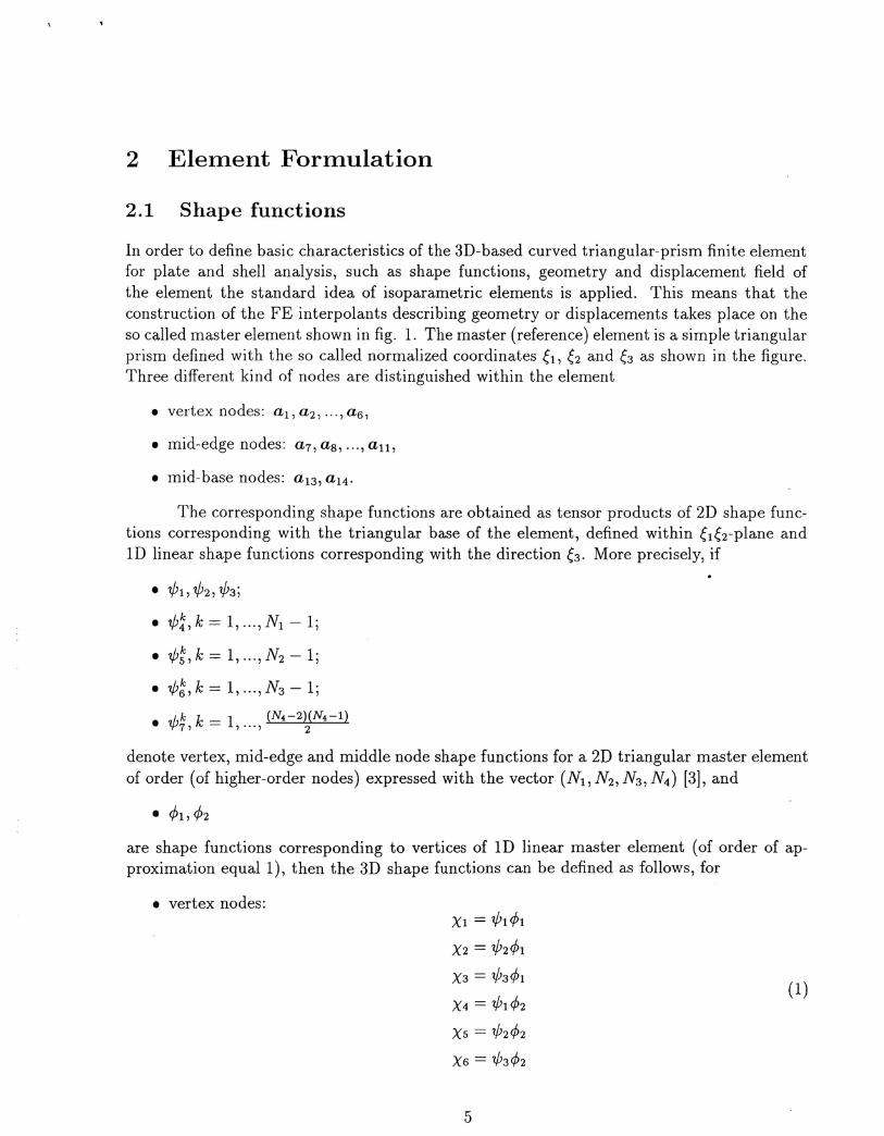
In order to define basic characteristics of the 3D-based curved triangular-prism finite elementfor plate and shell analysis, such as shape functions, geometry and displacement field ofthe element the standard idea of isoparametric elements is applied. This means that theconstruction of the FE interpolants describing geometry or displacements takes place on theso called master element shown in fig. 1. The master (reference) element is a simple triangularprism defined with the so called normalized coordinates ~l, 6 and 6 as shown in the figure.Three different kind of nodes are distinguished within the element

• vertex nodes: aI, a2, ... , a6,

• mid-edge nodes: a7, as, ... , all,

• mid-base nodes: a13, a14'

The corresponding shape functions are obtained as tensor products of 2D shape func-tions corresponding with the triangular base of the element, defined within 66-plane andID linear shape functions corresponding with the direction 6. More precisely, if

• 'l/Jl, 'l/J2, 'l/J3;• 'l/J~, k = 1, , N1 - 1;

• 'l/J;, k = 1, , N2 - 1;

• 'l/J~, k = 1, , N3 - 1;

./,k k = 1 (N4-2)(N4-1)• 'fI7, , ... , 2

denote vertex, mid-edge and middle node shape functions for a 2D triangular master elementof order (of higher-order nodes) expressed with the vector (NI, N2, N3, N4) [3], and

• <PI, <P2are shape functions corresponding to vertices of 1D linear master element (of order of ap-proximation equal 1), then the 3D shape functions can be defined as follows, for

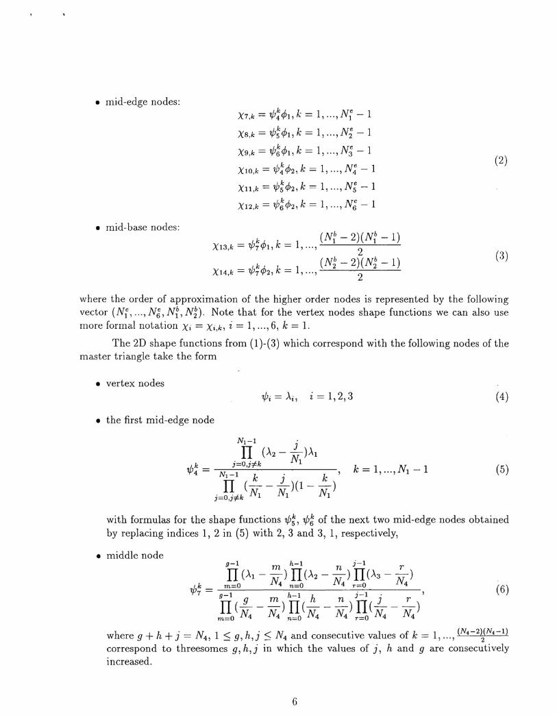
• vertex nodes:Xl = 'l/Jd>lX2 = 'l/J2<PlX3 = 'l/J3<PlX4 = 'l/Jl<P2XS = 'l/J2<P2X6 = 'l/J3<P2

5

(1)

• mid-edge nodes:

• mid-base nodes:

X7,k = 1/J:<Pl, k = 1, , N: - 1

X8,k = 1/;~<P1,k = 1, ,N;-1

X9,k = 1/;~<P1' k = 1, , N; - 1

XlO,k = 1/J:<P2,k = 1, ,N:-1

Xll,k = 1/J~<P2' k = 1, , N; - 1

X12,k = 1/J~<P2' k = 1, , N~- 1

X13,k = 1/;;<P1, k = 1, , (Nt - 2)(Nt - 1)

X14,k = 1/J;<P2, k = 1, , (N~ - 2)(N~ - 1)

(2)

(3)

where the order of approximation of the higher order nodes is represented by the followingvector (N:, ... , N6, Nt, N~). Note that for the vertex nodes shape functions we can also usemore formal notation Xi = Xi,k, i = 1, ... ,6, k = 1.

The 2D shape functions from (1)-(3) which correspond with the following nodes of themaster triangle take the form

• vertex nodes

• the first mid-edge node

1/;i = Ai, i = 1,2,3 (4)

k = 1, ... , N1 - 1 (5)

with formulas for the shape functions 1/;;, 1/;~ of the next two mid-edge nodes obtainedby replacing indices 1, 2 in (5) with 2, 3 and 3, 1, respectively,

• middle node9-1 m h-l n j-l rII(AI- -) I1(A2 - -) II(A3 --)

N N N1/;k = m=O 4 n=O 4 r~O 4 (6)7 9-1 h-1 h )-1' ,9 m n J rII(- --) II(---) II(---)

m=O N4 N4 n=O N4 N4 r=O N4 N4

where 9 + h + j = N4, 1 ~ g, h,j ~ N4 and consecutive values of k = 1, ... , (N4-2~(N4-1)

correspond to threesomes g, h,j in which the values of j, hand 9 are consecutivelyincreased.

6

..... a 1

a7./ a13~

Figure 1: Master triangular-prism shell finite element

Note, that we use so called affine (or area) coordinetes ),l, ),2,),3 iIi (4)-(6), which can beexpressed through normalized coordinates 6,6 with simple formulas: ),l = 6,),2 = 6 and),3 = 1- ~l - 6·

The form of the ID shape functions appearing in (1)-(3) and corresponding with twovertex nodes are defined as follows

(7)

2.2 Geometry definition

2.2.1 Geometry interpolant

We apply the idea of isoparametric geometry representation for element formulation. Thatmeans that we apply for geometry approximation the same shape functions as for approx-imation of displacements. The total interpolant x = x(e-) describing coordinates x =col(XI, X2, X3) of any point of the element is a sum of three component interpolants cor-responding with the vertex, mid-edge, and mid-side nodes

(8)

The linear (vertex nodes) interpolant Xl (e-) is defined as a sum of products of the

7

local geometrical degrees of freedom di

corresponding shape functions1, .., 6 at the vertex nodes and the

6

x1(e) = LXi(e)di(x),i=l

(9)

where di = col(dl,i, d2,i, d3,d.The mid-edge nodes interpolant x2 is defined as a sum of products of the local ge-

ometrical degrees of freedom d6+i,k = d6+i,k (x), i = 1, ... ,6 at the mid-edge nodes and thecorresponding shape functions

6 N?-l

x2(e) = L L X6+i,k(e)d6+i,k(X),i=l k=l

(10)

where the vectors of local geometrical dofs are: d6+i,k = col(d1,6+i,k, d2,6+i,k, d3,6+i,k).

The mid-base nodes interpolant x3(e) is defined analogously by multiplication of theproper local geometrical dofs dl2+i,k = d12+i,k( x), i = 1,2 and the corresponding shapefunctions

2 (Nt-2)(N;b_1)j2

x3(e) = L L Xl2+i,k(e)d12+i,k(X),i=l k=l

where the local dofs vectors are: d12+i,k = col(d1,I2+i,k, d2,I2+i,k, d3,12+i,k).

2.2.2 Geometrical degrees of freedom

(11 )

Geometrical degrees of freedom introduced in the previous paragraph depend on x being agiven continuous function describing the real geometry of the element. The definition of thesedofs proposed here follows from convergence analysis for hp finite element methods and, forthe higher order dofs, takes advantage of local HJ-projections. Defined in this way degrees offreedom are hierarchical in the sense that they have to be calculated in a specific order, fromvertex through mid-edge, mid-base, and mid-side nodes to middle node. More precisely,

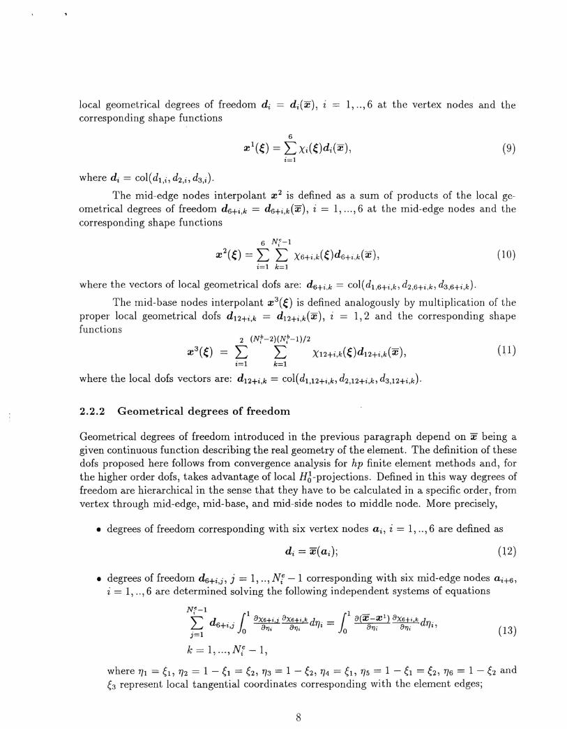
• degrees of freedom corresponding with six vertex nodes ai, i = 1, ." 6 are defined as

(12)

• degrees of freedom d6+i,j, j = 1, ..,Nt - 1 corresponding with six mid-edge nodes ai+6,i = 1, ..,6 are determined solving the following independent systems of equations

(13)

where 1]1 = ~I, 1]2 = 1 - 6 = ~2' 1]3 = 1 - ~2, 1]4 = 6,1]5 = 1 - 6 = 6,1]6 = 1 - 6 and6 represent local tangential coordinates corresponding with the element edges;

8

• degrees offreedom dl2+i,j, j = 1,.., (Nt -2)(Nt -1)/2 corresponding with two mid-basenodes ai+12, i = 1,2 are determined solving the systems of equations

(14)

k = 1, ..., (Nt - 2)(Nt - 1)/2.

Note, that each of three components of each geometrical degree of freedom correspond-ing with the element node can be calculated separately as each of the above sets of equationsconsists of three linearly independent subsets for each component.

2.3 Displacement field of the element

The total interpolant for approximation of the element displacement field, u = u(~), describ-ing displacements u = col(U1,U2, U3) of any point of the element is a sum of three componentinterpolants corresponding with the vertex, mid-edge, and mid-side nodes

(15)

The linear (vertex nodes) dispacement interpolant Ul(~) is defined as a sum of productsof the local degrees of freedom at the vertex nodes qi, i = 1, .. , 6 and the corresponding shapefunctions

6

Ul(~) = L Xi(~)qi'i=l

(16)

(17)

where qi = col(ql,i, q2,i, q3,i).

The mid-edge nodes interpolant of displacements U2(~) is defined as a sum of productsof the local degrees of freedom q6+i,k' i= 1, ... ,6 at the mid-edge nodes and the correspondingshape functions

6 N['-l

U2(~) = L L X6+i,k(~)q6+i,kli=l k=l

where the vectors of degrees of freedom are: q6+i,k = col(ql,6+i,k, Q2,6+i,k, q3,6+i,k).

The mid-base nodes interpolant of displacements U3(~) is defined analogously by mul-tiplication of the proper local degrees of freedom ql2+i,kl i = 1,2 and the corresponding shapefunctions

2 (Nt-2)(Nt-l)j2

U3(~) = L L X12+i,k(~)ql2+i,kli=l k=l

where the local dofs vectors are: ql2+i,k = COl(Q1,I2+i,k,Q2,12+i,k, Q3,12+i,k).

(18)

3 Numerical Procedures of the Element

The presented in the previous section shape functions as well as formulas describing geometryand displacement field of the element will be applied to formulation of standard characteristicsof the element such as stiffness matrix, body and surface load nodal vectors, etc. For theelement under consideration formulation of the stiffnesses and force vectors is not a standardone and thus it is presented in the report. The integrands representing each component ofthe stiffness matrix or load vector will be calculated numerically. Due to specific features ofthe applied numerical integration, it is described in one of the next subsections.

3.1 Stiffness matrix formation

The formulation of the stiffness matrix has to fulfill two general requirements. The first oneis that the element should be compatible with 3D hpq triangular-prism finite element (see[2] for the element definition). In this wayan analysis of generally arbitrary plate or shellproblems including multi-structures consisting of plate, shell and solid parts will be possiblewith the existing 3D adaptive package [4]. From the implementation point of view that meansthat the structure of the stiffness matrix (and also nodal forces vector) of the new elementfor the plate and shell analysis should be based on the same 3D degrees of freedom as appliedfor the 3D prismatic element, i.e. on the displacement degrees of freedom defined in theglobal Cartesian system of coordinates. On the other hand, we have the second requirement.The stiffness matrix has to represent well the plate or shell character of the structure. Aswe assumed that the transverse order of approximation is equal 1 then in order to avoidthe improper limit phenomena (see [2] for thorough explanation) the standard 3D approachhas to be enriched with the shell assumptions of plane stress and plane strain (compare also[5] where the plate case is analytically explained). This enrichment needs formulation ofthe element in the local coordinate system with one axis normal and two axes tangent to theshell longitudinal directions. The compromise between these two requirements is possible andwas proposed by the author in the context of classical formulation of 3D-based shell finiteelements [6]. Note that this approach is somehow similar but not identical to the approachapplied to standard thick shell finite elements [7, 8].

The stiffness matrix K of the new hp 3D-based element for plate and shell analysis isdefined with the following formula

rl r1 r-6+1 TK = Jo Jo Jo B D Bdet( J) d6d6d6, (19)

where B, D, and det( J) stand for the strain-displacement matrix, elasticity matrix andJacobian matrix determinant, respectively.

The strain-displacement matrix B is a differential operator matrix defined in the localCartesian coordinate system with one axis normal and two axes tangent to the coordinatesurface 66 of the curvilinear system of coordinates 6, 6, and 6 (equivalent to the normalizeddirections of the master element) and acting on the vector of element degrees of freedom q.

1(\

This vector consists of the vectors: qi, i = 1, ..,6; q6+i,k, i = 1, ..,6, k = 1, ..,Nt -1; Ql2+i,

i= 1,2, k = 1, .., (Nib - 2)(Nt - 1)/2 defined in subsection 2.3. Note that this matrix can bedivided into blocks corresponding to vertex, mid-edge, and mid-base nodes

(20)

These blocks can be divided into sub-blocks corresponding with the degrees of freedom definedfor each node, i.e.

(21)

Each sub-block of (21), Bj,k, where for the consecutive values j = 1,2, ..,14 we have eitherj = i, i = 1, .., 6, k = 1 or j = 6 + i, i = 1, ..,6, k = 1, .., Nt - 1 or j = 12 + i, i = 1,2,k = 1, .., (Nt - 2)(Nt - 1)/2, takes the following form

B11 B12 Bl3

B21 B22 B23

B31 B32 B33 I (22)B'k = I .J, B41 B42 B43

B51 B52 B53

B61 B62 B63

For the general 3D stress and strain states the elasticity matrix D utilizing Young'smodulus E and Poisson's ratio v is usually assumed to be equal to

I-v v v 0 0 0v I-v v 0 0 0

D- E I v v I-v 0 0 0 I . (23)- (1 + v)(l - 2v) 0 0 0 (1 - 2v)/2 0 0

0 0 0 0 (1 - 2v)/2 0

0 0 0 0 0 (1-2v)/2

3.1.1 Strain-displacement matrix calculations

Strain-displacement matrix terms. The components Bmn, m = 1,2, ..,6, n = 1,2,3 ofthe each sub-block B j,k of the strain-displacement matrix are defined as follows

(24)

11

where ()np, P = 1,2,3 represent terms of the matrix () transforming the the local directions ofthe shell into global Cartesian ones and auxiliary terms aj,k, aj,k, Cj,k are calculated from

aj,k = Al1Pl,j,k + A12P2,j,k + A13P3,j,k,

bj,k = A2IPl,j,k + A22P2,j,k + A23P3,j,k, (25)

The terms Pr,j,k, r = 1,2,3 in the above relations denote the derivatives of the shape functionswith respect to the normalized (or curvilinear) coordinates while the terms Ast, s, t = 1,2,1of the auxiliary matrix A are

A ()·It () ·2t () ·3tst = IsJ + 2sJ + 3sJ , (26)

where jrt are the terms of the inverse Jacobian matrix and ()ps are the terms of the transfor-mation matrix again.

Shape function derivatives. The formulas for derivatives of the shape functions Xj,k withrespect to normalized directions 6, 6, 6, where for the consecutive values j = 1,2, .. , 14 wehave either j = i, i = 1, .. ,6, k = 1 or j = 6 + i, i = 1, .. ,6, k = 1, .. , Nt - 1 or j = 12 + i,i = 1,2, k = 1, .. ,(Ni

b-2)(Nf-1)/2, are obtained with thegeneralrelationpr,j,k = aXj,k/a~r'r = 1,2,3, i.e.

aXi .Pr,i,l = aer' ~ = 1, ... ,6;

aX6+i,k .Pr,6+i,k = "'... , ~= 1, ... 6, k = 1, ... , Nt - 1;

(27)

(28)

i = 1,2, k = 1, ... , (Nf - 2)(Nib

- 1)2

(29)

Jacobian matrix. The terms jpr of the Jacobian matrix J can be obtained from the stan-dard definition jpr = aXr/ aep remembering definitions (8)-(11) of the geometry interpolant,1.e.

6 6 Nt-l 2 (N;b_2)(Nt-1)/2

jpr = LPp,i,ldr,i + L L Pp,6+i,kdr,6+i,k + L L Pp,l2+i,kdr,l2+i,k. (30)i=l i=l k=l i=l k=l

The terms rt of the inverse Jacobian marix can be otained by taking J-l and thanby using relations (30). The same relations can applied also for standard calculations of theJacobian matrix determinant det( J).

10

Transformation matrix. In order to determine the transformation matrix terms Gnp trans-forming the the local directions of the new shell element into global Cartesian ones let usdefine the three local directions at any point of the element. The normal direction will bedefined with vector W which is assumed to be perpendicular to the 66-plane. The next twodirections, which are tangent to this plane, are defined with the vectors U and V. The firstof them is assumed to coincide with the coordinate line of 6, while the second one can beobtained by vector multiplication of two previous vectors. Note that such definitions enableto express all three vectors in terms of the Jacobian matrix components, i.e.

W=[

~12~23- ~22~131- )21)13 - )11J23 ,

.. ..)11)22 - )21J12

(31)

[

(j2ti13 - j11j23)jI3 - j12(j11j22 - hlj12) jV = W x U = (j11j22 - j21j12)j11 - j13(j12j23 - j22j13) .

(j12j23 - j22j13)j12 - jll (j21j13 - j11j23)

Subsequently, the transformation matrix () can be defined with the global componentsof the unit vectors: u = U jU, v = V jV, w = W jW as follows

(32)

3.1.2 Introduction of plane stress assumption

The above formulation of the stiffness matrix was based on the differance operator matrix(strain-displacement matrix) defined in the local coordinates of which one was normal and twowere tangent to the longitudinal directions of the shell (or plate), which the operator actedon the degrees of freedom defined in the global system of coordinates. Such an approach isequivalent to the standard formulation of 3D finite elements where both the operator anddegrees of freedom are defined as global. The justification of this equivalence is that the localdifference operator has been defined through invariant tensor transformation of the elementstrain energy from the global to local directions and the additional replacement of the localdofs with the global ones by means of the transformation matrix ().

As the above formulation is equivalent to standard 3D formulation and as we assumedvertical order of approximation to be equal to 1 then in the thin limit the element will sufferfrom the so called improper limit phenomenon. In order to avoid this phenomenon plane

1 ~

stress and plane strain assumptions have to be introduced. The plane stress assumptionreads 0'33 = 0, where the index 3 refers to the third local direction of the shell. Introductionof this assumption is equivalent to some modifications of the strain displacement matrix andelasticity matrix. In particular, the strain-displacement matrix sub-blocks (22) have to bechanged in the following way

Bll B12 B13

B21 B22 B23

Bj,k = I B41 B42 B43 I (33)

B5l B52 B53

B61 B62 B63

and the elasticity matrix terms and coefficient from (23) have to be modified as follows

1 v 0 0 0

v 1 0 0 0

D = E 21 0 0 (1 - v)/2 0 0 I . (34)I-v o 0 0 (1 - v)/2k 0

o 0 0 0 (1 - v)/2k

Note, that the remaining terms of the sub-block Bj,k are defined with the same formulasas before and that the shear strain energy correction factor k = 1.2 has been itroduced tothe new definition of D. This factor accounts for the fact that according to plate and sheartheories transverse shear strains are not constant as we enforce through the assumption thatthe vertical (transverse) order of approximation is equal to 1.

3.2 Nodal forces vectors generation

Let us assume a vector of nodal forces F of the new hp 3D-based shell finite element to be asum of the appropriate vectors due to body forces F B and surface traction Fs

(35)

Body forces nodal vector. The nodal vector due to body loading will be defined in thefollowing way

{I (I r6+1FB = Jo Jo Jo NT fdet(J) d~3d6d6, (36)

where Nand f denote shape function matrix and the body loading vector, respectively.

The shape function matrix N can be divided into blocks corresponding to vertex,mid-edge, and mid-base nodes

(37)

1 A

These blocks can be divided into sub-blocks corresponding with the degrees of freedom definedfor each node, i.e.

N6+i (38)

Each sub-block of (38), Nj,k, where for the consecutive values j = 1,2, .. , 14 we have eitherj = i, i = 1, ..,6, k = 1 or j = 6+i, i = 1, ..,6, k = 1, .. ,Nt -lor j = 12+i, i = 1,2,k = 1, .., (Nib - 2)(Nib - 1)/2, takes the following form

(39)

For the case of gravitional load the vector of body loading f utilizing the elementdensity p and gravitional constant 9 can be defined in the form

(40)

(41)

Surface tractions nodal vector. The nodal vector due to surface tractions will be definedas follows

Fs =1111

NT pwsp(J) d6dTfi

(I r6+1Fs = Jo Jo NT pwsp(J) d6del

for the element sides and bases, respectively. In the above relations 6, 6, 6 denote thenormalized directions while "1i, i = 1,2,3 stand for the tangential coordinates defined. insection 2.2. The terms p and wsp( J) are the surface traction vector and the coefficient ofthe Jacobian matrix defined by

wsp(J) = (EG - F)I/2, (42)

where the auxiliary terms E, F, and G can be expressed through the Jacobian matrix terms

·2 ·2 ·2E = Jpl + Jp2 + Jp3

·2 ·2 + ·2G = Jrl + Jr2 Jr3

1 r:;

(43)

with the indices 1, 2, 3 corresponding to the global directions and indices r, p correspondingwith two curvilinear (either normalized or tangential) directions from equation (41).

For two cases considered in this report, of the vertical and normal surface loads, thevector of surface tractions p will be defined with the pressure q. For the case of verticalpressure we may have

(44)

while for the case of normal pressure we may assume

(45)

where A, B, and C defining the direction normal to the surface can be expressed with theJacobian matrix terms again

(46)

3.3 Imposing plane strain constraints

Imposing the plane strain assumption C33 = 0, where the index 3 refers to the third localdirection of the shell, is much more complex procedure than introduction of the plane stressassumption. Let us notice at first that because of the linear variation of displacements throughthe thickness the above assumption can be replaced by the constraints of constant normaldisplacements. That needs replacement of the displacements defined in the global Cartesiancoordinates by generalized displacements defined in the local systems with one axis normaland two axes tangent to the shell mid-surface, defined by the equation e3 = 1/2, for example.Note, that such a choice of the local system will produce no additional error if the geometryof the new 3D shell element is defined properly, i.e., the element sides are perpendicular toits mid-surface.

3.3.1 Replacement of dofs

Replacement of the globally defined displacements q with the globally defined generalizeddisplacements qI is formally equivalent to creating the element equilibrium equation in theform

KlqI = F1, (47)

in which vector qI consists of the component vectors qf = Hqi + q3+i), q~+i = Hqi - q3+i)'i = 1,2,3; q~+i = Hq6+i+q9+i), q~+i = i(q6+i-q9+J, i = 1,2,3; q{2+i = t(q12+i+

q13+i), qi3+i = Hql2+i - qI3+J, i = 1, and the terms of matrix K1 and of vector F1 areobtained through standard method of symmetric addition or subtraction of the proper rowsand columns of matrix K and proper rows of vector F, which the columns and rows refer tothe corresponding degrees of freedom of the top and bottom vertex, mid-side, and mid-basenodes.

3.3.2 Transformation of dofs

Temporary transformation of dofs as well as enforcement of the constraint and backwardtransformation of dofs described in next two subsections is necessary for any particular con-straint corresponding to the degree of freedom defined with m and 1. For the consecutivevalues of I and m we have either 1= i,i = 4,5,6, m = lor 1= 6+i, i = 4,5,6, m = 1, .. , Nic-lor 1= 12 + i, i = 2, m = 1, .. , (Nt - 2)(Ni

b - 1)/2.

Transformation of the globally defined generalized displacement dofs of the element,qI, to their locally defined generalized couterparts qII needs introduction of the transf~r-mation matrix A such that qI = AqII. In this way the equation of element equilibriumKlqI = F1 after its left multiplication by AT will take the form

(48)

which after introduction of the appropriate notation will give us the equation of the elementequilibrium in terms of the redefined displacement qII in the form K II qII = FII. Note thath II' f h t . II - II . - 1 6' II . - 1 6t e vector q conSIsts 0 t e component vee ors. qi - qi,l, Z - , .. , , q6+i,k, Z - , .. , ,

k = 1, .. , Nt - 1; qg+i, i = 1,2, k = 1, .. , (Nt - 2)(Nt - 1)/2. The transformation matrix Acan be divided into diagonal blocks corresponding to vertex, mid-edge, and mid-base nodes

(49)

These blocks can be divided into diagonal sub-blocks corresponding with the degrees offreedom defined for each node, i.e.

Ai = I, i = 1,2,3

Ai = I, i = 4,5,6

A6+i diaglI, I";,,, IJ, i = 1,2,3x(Nf-l)

A6+i = diag[~, i = 4,5,6 (50)x(Nje-l)

Al2+i - diag[I, I, I, I, ... , I], i = 1, v ~

x(Nt-2)(Nt-l)/2

A12+i = diag[!,l,l,l,l,l, ...,IJ, i = 2,v

x (Nt-2)(Njb_I)/2

17

where sub-block I is the unity matrix and each sub-block [ takes the following form

[

1 1 1 ]1l,I,m l2,I,m l3,I,m

l = ~2l'l,m ~22'I,m ~23'I,m .

3l,l,m 32,I,m 33,I,m

(51)

In order to determine the terms lnp,l,m, n, p = 1,2,3 of the transformation matrix block [letus define at first three local directions at the nodal points of the element corresponding witheach particular 1 and m. These points coordinates 6,I,m and 6,I,m are those corresponding tothe definition of the shape functions of the 2D triangular master element [3], and coordinate6,I,m = 1/2 corresponds to the mid-surface of the 3D master element. Note that such a choicerequires that the horizontal orders of approximation at the corresonding top and bottom nodesare the same, i.e. Nt = N~+i = 1, i = 1,2,3; Nt = N;+i = Ni, i = 1,2,3; Nt = Nt+i = N4,

i = 1. Let us now define three local directions at each of these points. The third directionwill be defined with vector W1,m which is assumed to be perpendicular to the shell or platemid-surface. The next two directions, which are tangent to this surface, are defined withthe vectors U I,m and V I,m' The first of them is assumed to lie in the Xl x3-coordinate plane,while the second one can be obtained by vector multiplication of two previous vectors. Suchdefinitions enable to express all three vectors in terms of the Jacobian matrix components,l.e.

[.. .. ]JI2,I,mJ23,I,m - J22,I,mJ13,I,m

W1,m = ~21,I,m~13,I,m- ~1l,I,m~23,I,m ,

In,l,mJ22,I,m - J2l,l,mJ12,I,m

[

jll,l,mj22,I,m - j21,I,mjI2,I,m ]

U1,m = 0 ,.. ..

J22,I,mJI3,I,m - J12,I,mJ23,I,m

(52)

V1,m = WI,m X U1,m.

Subsequently, the transformation matrix block [ can be defined with the global componentsof the unit vectors: UI,m = U1,m/UI,m, VI,m = V1,m/Vl,m, WI,m = WI,m/WI,m as

[

Ul,l,m VI,I,m

[= U2,I,m V2,I,m

U3,I,m V3,I,m

3.3.3 Enforcement of the constraint

Wl,l,m]W2,I,m

W3,I,m

(53)

The general form of the constraint of constant normal displacement is:

U~I(el m) = 0, (54),

where el,m = (6,I,m, 6,I,m, ~), ull = [T UI(el,m), uI = ~(U(6,I,m' 6,I,m, 1) - U(6,I,m,6,I,m, 0)).Using relations (15)-(18) as well as definitions (1)-(3) and (7) we can express left side of (54)

1 Q

as follows3

L 1/Ji(6,I,m, 6,I,m)q{~+ii=l

3 Nje-l

+ L L 1/J3+i,k(6,I,m,6,I,m)qi~+i,ki=l k=l

1 (Nt-2)(Njb-l)/2

+ L L 1/J6+i,k(6,I,m,6,l,m)qg3+i,k'i=l k=l

(55)

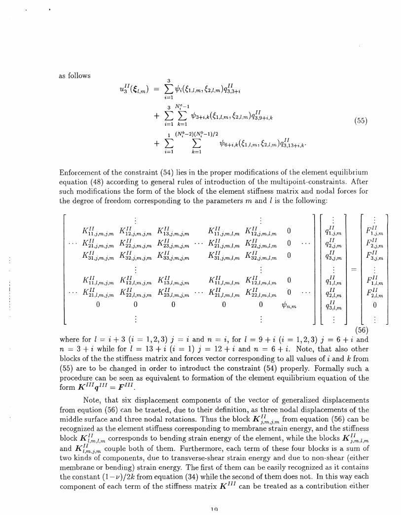
Enforcement of the constraint (54) lies in the proper modifications of the element equilibriumequation (48) according to general rules of introduction of the multipoint-constraints. Aftersuch modifications the form of the block of the element stiffness matrix and nodal forces forthe degree of freedom corresponding to the parameters m and l is the following:

[{II. . [{II. . [{II. . [{II [{II 0 II pII11,J,m,J,m l2,J,m,J,m 13,J,m,J,m ll,j,m,l,m 12,j,m,l,m ql,j,m 1,J,m

[{II .. [{II .. J{II. . [{II [{II 0 II pII... . .. q2,j,m2l,J,m,J,m 22,J,m,J,m 23,J,m,J,m 21,j,m,l,m 22,j,m,l,m 2,j,m[{II. . [{II [{II. . [{II [{II . 0 II pII

31,J,m,J,m 32,j,m,j,m 33,J,m,J,m 31,j,m,l,m 32,J,m,l,m q3,j,m 3,J,m

-[{II . [{II . [{II . [{II [{II 0 II FII

11,I,m,J,m 12,I,m,J,m 13,I,m,J,m ll,l,m,l,m 12,I,m,l,m ql,l,m l,l,m[{II . [{II . [{II ... [{II [{II 0 . .. II pII

2l,l,m,J,m 22,I,m,J,m 23,I,m,j,m 21,I,m,l,m 22,I,m,l,m q2,I,m 2,I,m

0 0 0 0 0 1/Jn,mII 0q3,I,m

(56)where for l = i + 3 (i = 1,2,3) j = i and n = i, for l = 9 + i (i = 1,2,3) j = 6 + i andn = 3 + i while for l = 13 + i (i = 1) j = 12 + i and n = 6 + i. Note, that also otherblocks of the the stiffness matrix and forces vector corresponding to all values of i and k from(55) are to be changed in order to introduct the constraint (54) properly. Formally such aprocedure can be seen as equivalent to formation of the element equilibrium equation of theform KIIlqIII = pIlI.

Note, that six displacement components of the vector of generalized displacementsfrom eqution (56) can be traeted, due to their definition, as three nodal displacements of themiddle surface and three nodal rotations. Thus the block K;,~,j,m from equation (56) can berecognized as the element stiffness corresponding to membrane strain energy, and the stiffnessblock Kf,;"',l,m corresponds to bending strain energy of the element, while the blocks K;,~,l,m

and Kf,;"',j,m couple both of them. Furthermore, each term of these four blocks is a sum oftwo kinds of components, due to transverse-shear strain energy and due to non-shear (eithermembrane or bending) strain energy. The first of them can be easily recognized as it containsthe constant (1- v) 12k from equation (34) while the second of them does not. In this way eachcomponent of each term of the stiffness matrix KIll can be treated as a contribution either

10

to the membrane, or bending, or transverse-shear strain energies of the element. That allowsone to apply the so called selective reduced integration to the stiffness matrix generation,in which the different components of the stiffness matrix terms are integrated according todifferent numerical integration rules. We will return to this problem in the next subsection.

3.3.4 Backward transformation of dofs

In order to change the temporarily introduced locally defined generalized displacement dofsq III (or eqivalent q II) to the locally defined displacement dofs qI let us remember thatqII = )..T qI. Subsequently, the left multiplication of (58) by A gives

(57)

which can be formally written as KIV qI = FIV. Note that the difference between I<IV, FIV

and KI, FI is that the former account for the plain strain constraints while the latter donot.

3.3.5 Backward replacement of dofs

Having enforced the plane strain constraints and having performed backward transformationof dofs for all degrees of freedom defined with m and I we can change the locally defineddisplacement dofs q I into the globally defined displacement dofs q. Such a change needsbackward modifications of the stiffness matrix columns and rows as well as of nodal forcesvector rows. In particular the same columns and rows of matrix KIV and the same rows ofvector FIV, as those of matrix K and vector F from subsubsection 3.3.1, have to be addedand subtract in order to obtain the element equilibrium equation of the form

(58)

Note that the difference between the stiffness matrices and nodal forces vectors K, F andKV

, FV is that the latter account for the plain strain constraints while the former do not.

3.4 Gauss integration

Two Gauss integration rules are applied in this research. The first one is a standard 3Dintegration scheme, i.e., it is the same rule as applied to triangular-prismatic hpq finite element(see [2] for details). The only difference is that the order of vertical approximation q is here,for the plate and shell analysis, kept constant and equal to 1. Thus the number of Gaussintegration points in the transverse (vertical) direction will also be constant. The secondintegration rule utilized in this research corresponds with the selective reduced integration ofthe stiffness matrix, which the selective reduced integration is applied only to the stiffnessmatrix terms corresponding to shear and membrane strain energies (also the terms couplingmembrane and shear energies are included) defined in the previos subsection. The reduced

')(\

integration is not applied to the terms of the stiffness matrix corresponding to the bendingstrain energy of the element. The reason for application of the selective reduced integrationis to overcome locking phenomena (for explanation see [11]).

3.4.1 Standard integration

The utilized method of numerical integration takes advantage of the so called symmetricalGaussian quadrature rule for the triangle [12], applied to longitudinal normalized coordinates6 and 6 of the master triangle (or equivalent affine coordinates ),I, ),2 and ),3) and standardGauss integration rule applied to the third, transverse normalized coordinate 6 of the 1D lin-ear master element, which mixed together form 3D, symmetrical-standard-product Gaussianintegration scheme. Such an approach can be justified by the fact that the shape functionsof the prismatic element are defined as tensor products of 2D shape functions correspondingwith the triangular base of the master element and 1D linear shape functions correspondingwith its third direction. Thus, each integrand f(el, 6, 6) of the stiffness matrix and the bodyload vector can be integrated according to the rule

(59)

(60)

where Nfl, WZ,2, 6,k, ~2,k and wt, 6,1 are the number of Gauss points, Gauss point weight,and coordinates for the triangle as well as Gauss point weight, and coordinate for the thirddirection. Note, that the number of Gauss points in the third direction is contant and equalto 2. Its value can be obtained from q + 1 standard 1D Gauss integration rule for q = 1.Note also, that in the above relation the normalized coordinates of the Gauss points for thetriangle can be replaced with the corresponding affine coordinates ),l,k = 6,k, ),2,k = 6,k,),3,k = 1- 6,k - 6,k.

The above rule is used for the volume integration of the stiffness matrix and bodyload nodal vector integrands. For the surface load nodal vector integrands the 2D, eithersymmetric Gaussian or standard Gaussian integration rules are utilized for the element basesand the element sides, respectively. They are defined as follows

N1•2rl r-6+1 1 GJo Jo f(el, 6)d6d6 = 2 E WZ,2f(6,k, 6,k),

11 1 2 Nor f('Tfi,6)d'Tfid6 = LLwtw~J('Tfi,k,6,1)

o Jo I=l k=l

In the first equation, f(6,6) = f(~I'~2,e~) with e~being the given third coordinate of abase, equal 0 or 1. In the second equation 'Tfi,i= 1,2,3 and 6 denote the tangential and thethird direction coordinates of the element side i with 1Ji= 1Ji(6,6) where for i = 1,6 = 0,for i = 2, 1 - el - ~2= 0 and for i = 3, 6 = O. Terms Nb, wi, 1Ji,k,the number 2, and theterms wt, 6,1 denote the number of Gauss points, Gauss point weight and coordinate for thetangential and third directions, respectively.

?1

The number of Gauss points for the triangle and the tangential direction, as well asthe corresponding numbers N~~~ and Njo! of single degrees of freedom for the consecutivevalues of the order of approximation, order, for the case when Nl = N2 = N3 = N4 = orderare the following

• order = 1, NI,2 _ 3, NI,2 _ 3, Ni Ni - 2'G - do! - G = do!- ,

• order = 2, Nl,2 _ 6, Nl,2 _ 6, Ni - Ni - 3,G - do! - G - do!- ,

• order' = 3, Nb,2 = 12, Nd~~ = 10, No = Njo! = 4',

• order = 4, Nb,2 = 16, Nd~~ = 15, Nb = Njo! = 5',

• order' = 5, Nb,2 = 25, Nd~~ = 21, Nb = Njo! = 6',

• order = 6, Nb,2 = 33, N~~~ = 28, Ni - Ni - 7'G - do!- ,

• order = 7, Nl,2 - 42 Nl~~ = 36, Ni - Ni - 8,G - , G - do!- ,

• order = 8, N1,2 - 61 Nd~} = 45, Ni - Ni - 9'G - , G - do!- ,

• order = 9, Nb,2 = 73, N~~~ = 55, No = Njo! = 10.


The general formula (59) for 3D symmetrical-standard-product Gaussian integration rule isalso valid in case of the selective reduced integration. The main difference is that the numberof Gauss points in the case of the reduced integration is lower than the corresponding numberof points in the standard case. Note, that only the number of Gauss points for the trianglehas to be changed while the number of the Gauss points in the third direction remains equalto 2. The reduced numbers of Gauss points for the triangle and the corresponding numbersNl~~of single degrees of freedom for the consecutive values of the order of approximation,order, for NI = N2 = N3 = N4 = order are the following

• order = 1, NI,2 _ 1, N1,2 _ 3,G - do! - ,

• order = 2, NI,2 _ 3, NI,2 _ 6'G - do! - ,

• order = 3,N1,2 _ 4, N~~} = 10;G -

• order' = 4, NI,2 _ 7, Nl~~ = 15;G -

• order = 5, N1,2 - 12 Nd~} = 21;G - ,

• or'der- = 6, Nb,2 = 16, Nd~} = 28;

22

d 12 Nl~~ = 36;• or er = 7, N d = 25,

• order = 8, N~,2 = 33, Nl~~ = 45;

• order = 9, N~,2 = 42, Nl~~ = 55.

The above numbers were established by the author through numerical tests (those numberswhich coped best with locking phenomena were chosen). The general rule for establishi.ngthese numbers for each particular value of O1'der is that N ~,2 (order) is the greatest or almostthe gratest value from the set of possible numbers of Gauss points for the triangle establishedin [12] that satisfies the relation N ~,2 (01'der) ~ N l~~(order - 1).

Note, that due to the last relation locking can be expected to be removed but. theobtained solution values may be overestimated (the stiffness may become too small when therelation N~,2(order) < Nl~~(order - 1) holds). That is why the case when N~,2(01'der)is the smallest or almost the smallest value from the set of possible numbers of Gausspoints that satisfies the opposite relation N~,2( order) 2: Nl~~( order - 1) will also be an-alyzed. Note that removing of locking cannot be expected to be total when the relationN~,2( order) > Nl~~( orde1' - 1) holds. The reduced numbers of Gauss points for the triangleand the corresponding numbers Nl~~of single degrees of freedom for the consecut.ive valuesof the order of approximation, order, for N1 = N2 = N3 = N4 = order for that case are thefollowing

• order = 1, N~,2 = 1, NI,2 _ 3,do! - ,

• order = 2, N~,2 = 3, NI,2 _ 6'do! - ,

• order = 3, Nb,2 = 6, Nl~~ = 10;

• order = 4, N~,2 = 12, NJ~~ = 15;

• order = 5, Nb,2 = 16, Nl,2 - 21'do! - ,

• order = 6, N~,2 = 25, Nl~~ = 28;

• order = 7, Nb,2 = 33, NJ~~ = 36;

• order = 8, Nb,2 = 42, Nl~~ = 45;

• order = 9, lVb2 = 61, NJ~~ = 55.

There also exist other choices of the numbers N~,2 from the set of possible numbers of Gausspoints for the triangle.

4 Methodology of the Numerical Research

4.1 Three plate and shell problems

Three exemplary plate and shell problems are considered in the report. The first one is aproblem of a rectangular plate with clamped edges, loaded with transverse uniform surfacetraction. The plate problem has been chosen as due to lack of curvature the membranestrain energy of the plate (if any) is not coupled with the bending and transverse shear strainenergies through longitudinal and transverse displacement fields, thus no membrane lockingis expected for that example. Note, however, that shear locking may apper for the plate inthe thin limit (see [2] for explanation). Furthermore, the choice of clamped edges togetherwith lack of any longitudinal loading ensures that the membrane strain energy equals zero.Additionally, the type of loading permits for obtaining analytical solution of the problem.

The next two examples considered in this report deal with shell problems. The firstof them is a half-cylindrical shell with clamped, horizontally placed straight edges and withfree curved edges, loaded with vertical uniform surface traction. Due to the chosen bound-ary conditions and normal component of the loading changing along the curved edges themembrane part of the total strain energy almost vanishes when thickness of the shell tendsto zero (compare [14] where the analytical proof for a very similar example is given). Asthe bending strain energy has a tendency to be much greater than the membrane part thisexample can be called a bending-dominated shell problem (see [2] for more details). Note,that in the same sense the plate problem presented above is also a bending-dominated one.The bending-dominated shell problem described here is especially interesting as both shearand membrane lockings (or should we say membrane-shear locking) may appear (compare [2]again).

The third problem which is a second shell problem is a cylindrical shell without rotationalong the curved edges, loaded with the uniform internal pressure. Due to axisymmetry ofthe geometry and uniformity of the loading there is no variation of displacements along thecylinder circumference. If the shell is long enough and its thickness is small also there isno change of displacemnts along the direction of the shell longitudinal axis apart from thevicinity of the boundaries. Thus one can predict that there is almost no bending and sheardeformations for this example (see [10] for more detailed arguments). As the membrane energydominates the bending energy of the shell the problem can be called a membrane-dominatedshell problem (see [2] for more precise definition). Note, that this is a global characteristicsof the problem as locally, near the boudaries, bending deformations may apper. We shouldmention that the assumed boundary conditions allow one to obtain the analytical solutionof the problem. This example is especially interesting as no locking can be expected (see [2],where the explanation is presented).

Rectangular plate with clamped edges. According to the classical thin plate theory(Kirchhoff theory) [10] the equilibrium of the rectangular plate under vertical surface loading

')4

(62)

(63)

a

Figure 2: Rectangular plate geometry and loading

q = q(XI' X2) (fig. 2) can be described with the following differential equation

8tU3 + 28;8;U3 + 8~U3 = q(XI,X2)/D. (61)

The coefficient D is defined as follows D = Et3/[12(1 - v2)], where t denotes the thickness ofthe plate, E is Young's modulus and v is Poisson's ratio. The indices 1,2 and 3 correspondto two longitudinal and one transverse directions of the cartesian coordinates Xl, X2, X3.

The analytical solution for maximal, central deflection, (U3)max, obtained for thesquare plate under the uniform load, q = const, and clamped boundary conditions

U3 = 0, 82U3 = 0, for Xl = ± a/2

U3 = 0, 8lU3 = 0, for X2 = ± a/2,where a is the length of each side of the plate, is given by [10]

5qa4 4qa4 = (-1 )(m-l)/2 am tanham + 2(U3)max = 384D - 5D L: 5 2 h

1f m=1,3,.. m cos am

~4 f= Em( _1)(m-I)/2 a~ tanham1f D m=1,3,.. m cosham

qa4

0.00126 D'

where am = m1f/2 and Em are coefficients depending on loading and boundary conditions.

?I)

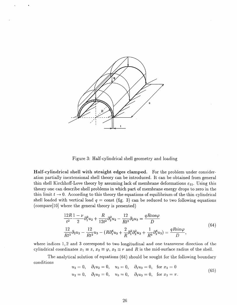
Figure 3: Half-cylindrical shell geometry and loading

Half-cylindrical shell with straight edges clamped. For the problem under consider-ation partially inextensional shell theory can be introduced. It can be obtained from generalthin shell Kirchhoff-Love theory by assuming lack of membrane deformations Cll. Using thistheory one can describe shell problems in which part of membrane energy drops to zero in thethin limit t --7 O. According to this theory the equations of equilibrium of the thin cylindricalshell loaded with vertical load q = const (fig. 3) can be reduced to two following equations(compare[10] where the general theory is presented)

(64)

where indices 1,2 and 3 correspond to two longitudinal and one transverse direction of thecylindrical coordinates Xl = Z, X2 = cp, X3 == rand R is the mid-surface radius of the shell.

The analytical solution of equations (64) should be sought for the following boundaryconditions

U2 = 0, 81U2 = 0, U3 = 0, 81U3 = 0, for X2 = 0

U2 = 0, 8lU2 = 0, U3 = 0, 8lU3 = 0, for X2 = 7r.

26

(65)

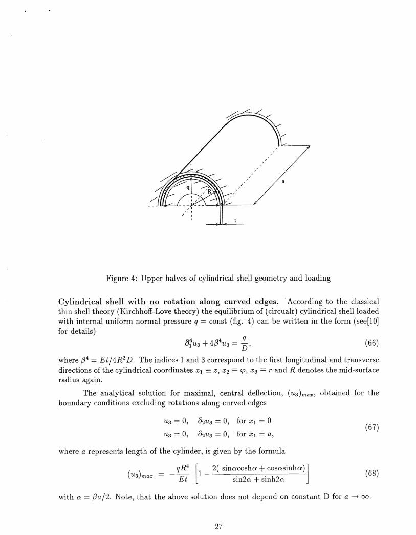
Figure 4: Upper halves of cylindrical shell geometry and loading

Cylindrical shell with no rotation along curved edges. .According to the classicalthin shell theory (Kirchhoff-Love theory) the equilibrium of (circualr) cylindrical shell loadedwith internal uniform normal pressure q = const (fig. 4) can be written in the form (see[10]for details)

8iu3 + 4{34u3 = ~, (66)

where {34 = Et/4R2 D. The indices 1 and 3 correspond to the first longitudinal and transversedirections of the cylindrical coordinates Xl == Z, X2 = <p, X3 - rand R denotes the mid-surfaceradius again.

The analytical solution for maximal, central deflection, (U3)max, obtained for theboundary conditions excluding rotations along curved edges

U3 = 0, 82U3 = 0, for Xl = 0

U3 = 0, 82U3 = 0, for Xl = a,

where a represents length of the cylinder, is given by the formula

) __ qR4 [1 _ 2( sinacosha + cosasinha)](U3 max E . 2 . h2t Sl11 a + Sl11 a

(67)

(68)

with a = {3a/2. Note, that the above solution does not depend on constant D for a --t 00.

27

4.2 Choice of calculation cases

The following geometrical data have been taken for all three examples: a = 3.14157.10-2 m2,

R = 1.0.10-2 m2 (note that 7fR~ a). Thickness of the plate (or shells) t was changed in thewide range; from 1.0.10-2 through 0.3.10-2, 0.1.10-2, 0.03·10-2, 0.01.10-2 up to 0.003.10-2

m. The corresponding ratios tj a were approximately equal to 33%, 10%, 3.3%, 1.0%, 0.33%and 0.1%, respectively. The Young's modulus E and Poisson's ratio v were taken as equalto 2.1 . lOll Njm2 and 0.3. The value of the loading q equaled 4.0.106 Njm2 for all threeexamples.

The calculation cases for each of three examples differed with the uniform horizontalorder of approximation p, uniform vertical order of approximation q and the uniform meshdensity characterized by the number m of longitudinal divisions of each of the plate (or shell)sides a or 7f R. The number of triangular-prism elements corresponding to parameter m isthus equal to 2m2. Note, that in the case of membrane-dominated shell only a half-cylinderwith proper symmetry boundary conditions was analyzed. The number of transverse divisionwas kept constant and equal to 1. For the plate example horizontal order of approximationwas taken as p = 1,2, ... ,8 and mesh parameter was m = 2,4,8,16,32. For the bending-dominated shell example we had p = 2,3, ... , 8 (p = 1 was analyzed for dense meshes, i.e.,when m ~ 8) and m was taken as in the case of plate example. For the membrane-dominatedcase p and m were changed as in the case of bending-dominated shell. The maximal valuesof p and m applied in this research were limited by the capabilities of the applied codes [4],[9].

In the convergence analysis the reference values 'of energies (playing a role of exactones) were taken from calculations of three examples of plate and shells performed for p ~ 6and m = 16.

In the displacement analysis of locking the values of displacements were scaled withthe factor proportional to t3 in the case of plate and bending-dominated shell examples andwith the factor proportional to t in the case of membrane-dominated shell. It can be noticedthat the values of (U3)max from (63) and (68) are proportional to t3 and t, respectively. Thereference values of central deflection for all three cases were taken from the same numericalcalculations as in the case of convergence analysis. In the plate and membrane-dominatedcases these values were compared with analytical ones. The differences between the best nu-merical values and analytical results of central deflection were meaningless for both examples.

5 Results of the Research

5.1 Rectangular plate

Presentation of the results for the plate example is limited to such problems as the lockingphenomenon (as a function of horizontal order of approximation p, mesh density parameterm, and thickness t), h- and p-convergence, sensitivity of the solution to the geometricalanisotropy of the mesh (due to triangular shape of the bases of the applied elements), andstability of the solution with decreasing thickness t of the plate.

5.1.1 h- and p-Convergence

In order to investigate h- and p-convergence of the applied uniform hp finite element methoda large number of cases for p = 1,2, ... ,8, m = 2,4,8, 16,32 were calculated. In order toillustrate p- and h-convergence two exemplary diagrams for a thin plate (t Ia = 0.33%) areprovided (figures 5 and 6). The error of approximation defined as a difference between thetotal strain energy J obtained numerically and its reference counterpart Jr playing a role ofan exact value of the energy (see subsection 4.2 for details) was plotted vs. number of degreesof freedom N for varying p and varying m in both diagrams. The locked values of energiesare those represented by horizontal or almost horizontal lines in the diagrams. The lockingphenomenon is also referred in next two subsections.

5.1.2 Shear locking effect

In order to investigate the shear locking phenomenon a large number of calculation cases werecomputed for p = 2,3, ... ,8 and m = 2,4,8. In order to visualize the influence of the orderof approximation p and mesh density parameter m on locking phenomenon two exemplarydiagrams (figures 7 and 8) are provided where the scaled values Ws of central deflection (U3)max

(see subsection 4.2 for scaling details) vs. thinness ratio alt are plotted for either varyingp (with m kept constant) or varying m (with p kept unchanged). The locked values of thesolution are those close to zero in both diagrams.


The calculations from the previous subsubsection were also repeated for the case of the firstreduced integration technique described in section 3.4. The corresponding curves of the scaledvalues Ws of central deflection (U3)max vs. thinness ratio alt are plotted for either varying p orvarying m again and shown in figures 9 and 10, respectively. It can be seen from comparisonof these figures to figures 7 and 8 that locking was totally removed for p = 3, however for thethin grid (h = 2) the solution values are slightly underestimated. For p = 2 locking was notremoved, however slight improvement of the result was obtained.

3.0

p=1

2.0

p=4

1.0

,.....,........!. 0.0-tillo-

-1.0

-2.0

-3.02.0 2.5 3.0 3.5

log N

p=2

4.0 4.5

..............m=2-....- m=4............m=6~m=16~m=32

Figure 5: p-Convergence curves for the plate (tja = 0.33%)

3.0 3.5log N

3.00

2.00

1.00

,.....,.......I 0.00.....-till~

-1.00

-2.00

-3.002.0

m=8 m=12 m=16 m=24 m=32• • •m=4

m=2~

~m~

m=4

2.5

m=12

4.0 4.5

-p=l-....- p=2...............p=3~p=4~p=6

Figure 6: h-Convergence curves for the plate (tja = 0.33%)

30

4.00

3.00

~.2.00

1.00

0.00 .1 10 100

Thinness ratio aft1000

.............p=1-p=2...............p=3IWHHH\ p=4.5.6,7.B

Figure 7: Scaled transverse deflection for the plate vs. p (m = 4, standard integration)

4.00

3.00

.;2.00

1.00

0.00 .1 10 100


.............m =2-m=4...............m=B

Figure 8: Scaled transverse deflection for the plate vs. m (p = 3, standard integration)

31

4.00

3.00

~2.00

1.00

0.00 .1 10 100


..............p=l

..............p=2

...............p=3IWWHI-A p=4.5.6.7.B

Figure 9: Scaled transverse deflection for the plate vs. p (m = 4, reduced integration)

4.00

3.00

~2.00

1.00

0.00 .1 10 100


..............m=2

..............m=4

...............m=B

Figure 10: Scaled transverse deflection for the plate vs. m (p = 3, reduced integration)

32

The same calculations were also repeated for the second reduced integration rule fromsection 3.4. In this case locking was not removed for any value of p and only slight advategouesimprovement of the results was observed, i.e., the locked values of the central deflection werehigher (but still locked) than those obtained with the standard integration.

5.2 Half-cylindrical shell


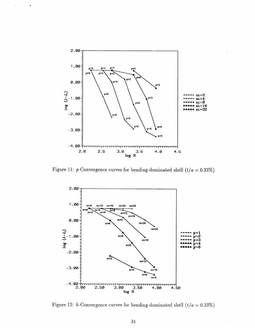
In order to investigate h- and p-convergence of the applied uniform hp finite element methoda large number of cases for p = 1,2, ... ,8, m = 2,4,8,16,32 were calculated. In order toillustrate p- and h-convergence two exemplary diagrams (figures 11 and 12) for a thin shell(t Ia = 0.33%) are provided. The error of approximation defined as a difference between thetotal strain energy J obtained numerically and its reference counterpart Jr playing a role ofan exact value of the energy (see subsection 4.2 for details) was plotted vs. number of degreesof freedom N for varying p and varying m in both diagrams. The locked values of energiesare those represented by horizontal or almost horizontal lines in the diagrams.

5.2.2 Membrane-shear locking effect

In order to investigate the membrane-shear locking phenomenon a large number of calcula.tioncases were computed for p = 2,3, ... ,8 and m = 2,4,8. In order to visualize the influenceof the order of approximation p and mesh density parameter m on locking phenomenon twoexemplary diagrams (figures 13 and 14) are provided where the scaled values Ws of centraldeflection (U3)max (see subsection 4.2 for scaling details) vs. thinness ratio alt are plotted foreither varying p (with m kept constant) or varying m (with p kept unchanged). The lockedvalues of the solution are those close to zero in both diagrams.


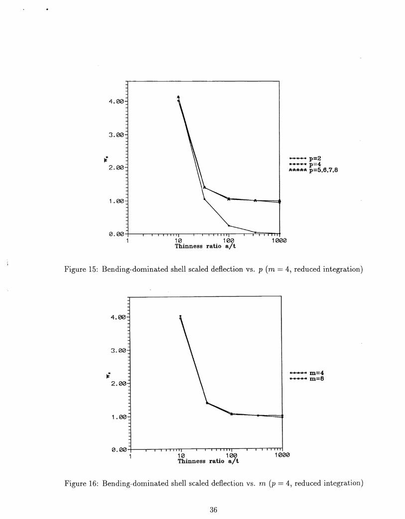
The calculations from the previous subsubsection were repeated for the case of the firstreduced integration technique described in section 3.4. The corresponding curves of thescaled values Ws of central deflection (U3)max vs. thinness ratio alt are plotted for eithervarying p or varying m again and shown in figures 15 and 16, respectively. It can be seenfrom comparison of these figures to figures 13 and 14 that locking was removed for p = 4.Note, however that for h = 2 the solution values were numerically unstable. For h = 4 and8 some traces of this instbility was also observed in the solution pattern. This phenomenonappeared to be extremally strong for p = 3. That is why no results for p = 3 and h = 2 areplotted in the diagrams.

The same calculations were also repeated for the second reduced integration rule fromsection 3.4. In this case locking was not removed for any value of p and only slight advategouesimprovement of the results was observed, i.e., the locked values of the central deflection were

33

2.00

............I2.. -1 .00

bIIo-

-2.00

-3.00

-4.002.0 2.5 3.0 3.5

log N

p=4

p=8

4.0 4.5

--- m=2~m=4--- m=B~m=16~m=32

Figure 11: p-Convergence curves for bending-dominated shell (tja = 0.33%)

2.00

.........;-..!. -1.00-

-2.00

-3.00

m=12 m=16 m=24 m=32

m=8

-p=l~p=2............--p=3~p=4........ p=B

-4.002.00 2.50 3.00 3.50

log N4.00 4.50

Figure 12: h-Convergence curves for bending-dominated shell (tja = 0.33%)

34

4.00

3.00

.;2.00

1.00

0.00 .1 10 100


..............p=2--p=3...............p=4IWWHH\ p=5.6.7.8

Figure 13: Bending-dominated shell scaled deflection vs. p (m = 4, standard integration)

4.00

3.00

.;2.00

1.00

0.00 .1 10 100


..............m=2--m=4...............m=8

Figure 14: Bending-dominated shell scaled deflection vs. m (p = 4, standard integration)

3.5

4.00

3.00

~2.00

1.00

0.00 .1 10 100


..........p=2

...............p=4~p=5.6.7.B

Figure 15: Bending-dominated shell scaled deflection vs. p (m = 4, reduced integration)

4.00

3.00

~2.00

1.00

0.00 .1 10 100

Thinness ratio aft

.............m=4~m=B

1000

Figure 16: Bending-dominated shell scaled deflection vs. m (p = 4, reduced integration)

36

higher (but still locked) than those obtained with the standard integration. The results werenumerically stable in this case.

5.3 Cylindrical shell


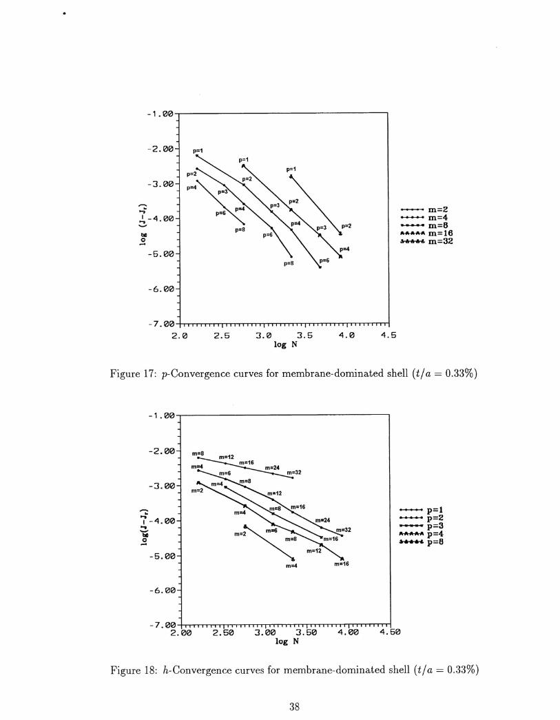
In order to investigate h- and p-convergence of the applied uniform hpq finite element methoda large number of cases for p = 1,2, ... ,8, m = 2,4,8,16,32 were calculated. In order toillustrate h- and p-convergence two exemplary diagrams (figures 17 and 18) for a thin shell(t Ia = 0.33%) are provided. The error of approximation defined as a difference between thetotal strain energy J obtained numerically and its reference counterpart Jr playing a role ofan exact value of the energy (see subsection 4.2 for details) was plotted vs. number of degreesof freedom N for varying p and varying m in both diagrams. There are no horizontal linesin the diagrams. That confirms lack of locking for the memebrane-dominated shell example.

5.3.2 Check on locking

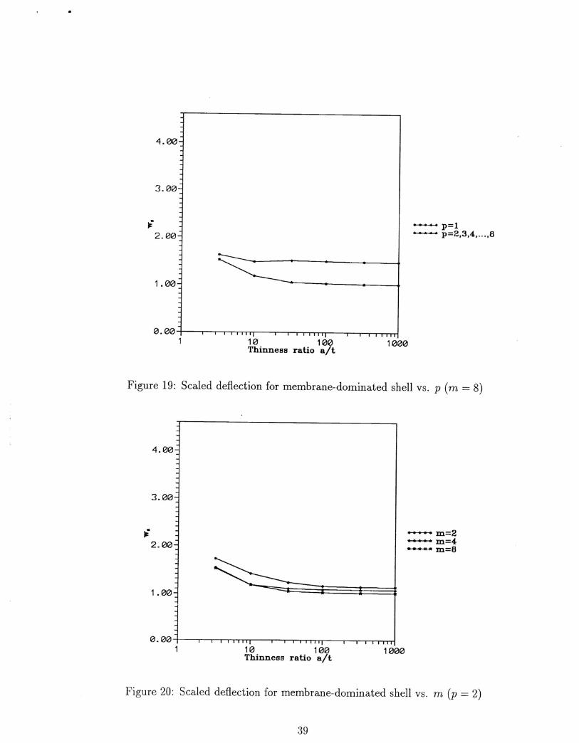
In order to investigate the existence of the locking phenomenon for the example of membrane-dominated shell a large number of calculation cases were computed for p = 1,2,3, ... ,8 andm = 2,4,8. In order to visualize the influence of the order of approximation p and meshdensity parameter m on the solution two exemplary diagrams (figures 19 and 20) are providedwhere the scaled values Ws of central deflection (U3)max (see subsection 4.2 for scaling details)vs. thinness ratio alt are plotted for either varying p (with m kept constant) or varyingm (with p kept unchanged). No locking effect does appear, i.e., none of the solution valuesshown in both diagrams is zero.

5.3.3 Influence of the reduced integration

We also check the influence of the reduced integration for the membrane-dominated shell.Note, that for such a shell the reduced integration is not necessary as there is no locking forthat case. The reason for the investigation was to check what is the response of the elementin case of the reduced integration applied for the membrane-dominated example.

In order to do so the calculations from the previous sub subsection were repeated forthe case of the first and the second reduced integration rules described in section 3.4. In thefirst case the results of the scaled values Ws of central deflection (U3)max vs. thinness ratioalt appeared to be numerically unstable in a wide range of p and h. In the second case noinstbility of ther solution pattern occured but the results were worse than those obtainedwith the standard integration, i.e., the tendency to overestimate the solution values appearedas a result of application of the second reduced integration rule.

37

-1.00

-2.00

-3.00

...........;J. -4.00.....,

-5.00

-6.00

...............m=2-...- m=4......-....m=6--m=16.Hr-6-+& m=32

-7.002.0 2.5 3.0 3.5

log N4.0 4.5

Figure 17: p-Convergence curves for membrane-dominated shell (tja = 0.33%)

-1.00

-2.00

-3.00

.........

7"-4.00.,~o-

-5.00

-6.00

m=4 m=16

-p=l-...- p=2-p=3--p=4........... P=8

-7.002.00 2.50 3.00 3.50

log N4.00 4.50

Figure 18: h-Convergence curves for membrane-dominated shell (tj a = 0.33%)

38

4.00

3.00

~.2.00

1.00

0.00 .1 10 100


"""""""'p=l-...- p=2.3.4 ..... B

Figure 19: Scaled deflection for membrane-dominated shell vs. p (m = 8)

4.00

3.00

.;2.00

1.00

0.00 .1 10 100


...............m=2

..............m=4

...........m=8

Figure 20: Scaled deflection for membrane-dominated shell vs. m (p = 2)

39

6 Discussion of the Results

6.1 Numerical sensitivity and stability of the element

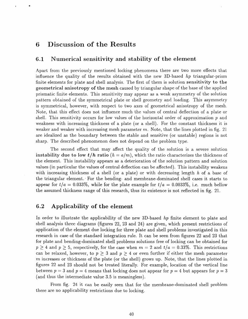
Apart from the previously mentioned locking phenomena there are two more effects thatinfluence the quality of the results obtained with the new 3D-based hp triangular-prismfinite elements for plate and shell analysis. The first of them is solution sensitivity to thegeometrical anisotropy of the mesh caused by triangular shape of the base of the appliedprismatic finite elements. This sensitivity may appear as a weak asymmetry of the solutionpattern obtained of the symmetrical plate or shell geometry and loading. This asymmetryis symmetrical, however, with respect to two axes of geometrical anisotropy of the mesh.Note, that this effect does not influence much the values of central deflection of a plate orshell. This sensitivity occurs for low values of the horizontal order of approximation p andweakness with increasing thickness of a plate (or a shell). For the constant thickness it isweaker and weaker with increasing mesh parameter m. Note, that the lines plotted in fig. 21are idealized as the boundary between the stable and sensitive (or unstable) regions is notsharp. The described phenomenon does not depend on the problem type.

The second effect that may affect the quality of the solution is a severe solutioninstability due to low tjh ratio (h = aim), which the ratio characterizes the thickness ofthe element. This instability appears as a deterioration of the solution pattern and solutionvalues (in particular the values of central deflection can be affected). This instability weakenswith increasing thickness of a shell (or a plate) or with decreasing length h of a base ofthe triangular element .. For the bending- and membrane-dominated shell cases it starts toappear for tla = 0.033%, while for the plate example for tla = 0.0033%, i.e. much bellowthe assumed thickness range of this research, thus its existence is not reflected in fig. 21.

6.2 Applicability of the element

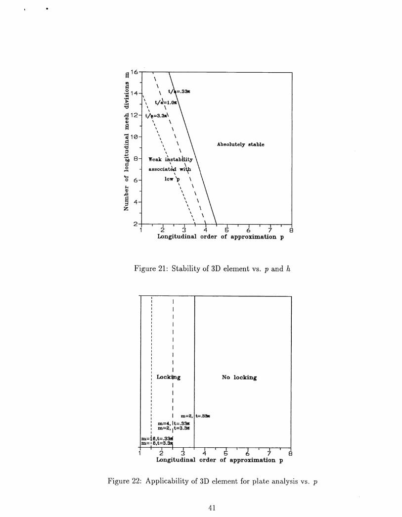
In order to illustrate the applicability of the new 3D-based hp finite element to plate andshell analysis three diagrams (figures 22, 23 and 24) are given, which present restrictions ofapplication of the element due locking for three plate and shell problems investigated in thisresearch in case of the standard integration rule. It can be seen from figures 22 and 23 thatfor plate and bending-dominated shell problems solutions free of locking can be obtained forp ~ 4 and p ~ 5, respectively, for the case when m = 2 and tla = 0.33%. This restrictionscan be relaxed, however, to p ~ 3 and p ~ 4 or even further if either the mesh parameterm increases or thickness of the plate (or the shell) grows up. Note, that the lines plotted infigures 22 and 23 should not be treated literally. For example, location of the vertical linebetween p = 3 and p = 4 means that locking does not appear for p = 4 but appears for p = 3(and thus the intermediate value 3.5 is meaningless).

From fig. 24 it can be easily seen that for the membrane-dominated shell problemthere are no applicability restrictions due to locking.

40

Absolutely stable

\\\ tJ_=.33l1

\

'- t/a'= l.0ll\ \\

th-=3.a.\'- \

'- \'- \'- \'- \Weak ~stabili.ty

\ \aS90ciB.t~ witf

\

low 'p \'- \

'- \'- \'- \'- \

\

2i 2 j 4 5 678

Longitudinal order of approximation p

.....o 6HIII.c~ 4Z

Qj10.S"Cl

B'bli 8I::lo-

Figure 21: Stability of 3D element vs. p and h

IIIIIIIIII

Lockilng I No lockingIIIII m=2.1 t=.3l111:

m=4.lt=.33l1m=2. It=3.3lI

m=i6.t=.3~m=16.t=3.~

I I I I I ' I I I I I I

12345 678Longitudinal order of approximation p

Figure 22: Applicability of 3D element for plate analysis vs. p

41

IIIIII

Locking

m=2. It=.3:R

No locking

m=4.1t=.3:Rm=2, t=3.:R

Ih=8. ;t=.3:R Ih=4.1t=3.:k

: I Im=:I2.t=.3~

i I I I I I I I I I ' I2 3 4 5 6 7 8

Longitudinal order of approximation p

Figure 23: Applicability of 3D element for bending-dominated shell vs. p

No locking

I i I I I I I ' I I I I

2 3 4 5 678Longitudinal order of approximation p

Figure 24: Applicability of 3D element for membrane-dominated shell vs. p

42

It should be stressed here that for each particular plate or shell problem the restric-tions of applicability due to locking should be confronted with the same restrictions due tosensitivity to geometrical anisotropy of the mesh. In other words, figures 22, 23 or 24 shouldbe always analyzed together with fig. 21 from the previous section. Note, that for plate andbending-dominated shell problems restrictions due to locking and due to element sensitivitysomehow coincide, i.e., occur for similar values of p.

43

..

7 Conclusions

Let us start with a very general conclusion concerning modelling features of the presentedelement. The novelty of the 3D-based finite element for plate and shell analysis lies in afact that the displacement field of the element is that corresponding to three-dimensionalcontinuum, while the the model coded in the element algorithms correspnds to Reissner-Mindlin plate and shell theories.

Another general conclusion is that each of three examples considered in this researchappeared to have different features, however there is some relevance between two bending-dominated examples (the plate and bending-dominated shell problems).

Conclusions dealing with either shear or membrane-shear locking phenomena occuringfor the plate, bending-dominated shell, and membrane dominated shell examples are thefollowing:

• Locking is an immanent feature of the bending-dominated examples (plate and firstshell examples) especially for low values of p and m.

• Shear locking (plate example) seems to be less severe than membrane-shear locking(first shell example).

• For the p-method, with t kept const, there always exists a number p depending on m,for which locking disappears.

• For the p-method (with m = const) there seems to exist the number p for whichdecreasing t does not lock the solution.

• For h-method there seems to exist a number m (depending on p, but also on t) for whichthe method unlocks. The tests performed by the author for t kept constant indicatethat even for p = 1 for the plate or p = 1,2 for the shell, the h-method has a tendencyto unlock, however, the number m must be increased dramatically, making the methoduneffective.

• For the h-method there does not exist any constant value of m for which the methodunlocks if alt grows faster than m. The tests revealed that for p ~ 3 in the plate caseand p ~ 4 in the shell case, with m = 4 (and p ~ 4 and p ~ 5, with m = 2, or p ~ 5 andp ~ 6, with m = 1), the solutions may be affected by locking (either by total lockingor its traces only) when t tends to zero.

• Summing up, p-method seems to be more effective in removing locking than h-method.

• Locking does not appear in the case of membrane-dominated shell example.

• It follows from comparison of the presented results with the results of [2] that for theplate example there is no difference in a tendency to lock of the presented elementand the 3D element acting under assumption q = 2. For the bending-dominated shell,however, the new element seems to be slightly more resistant to locking.

44

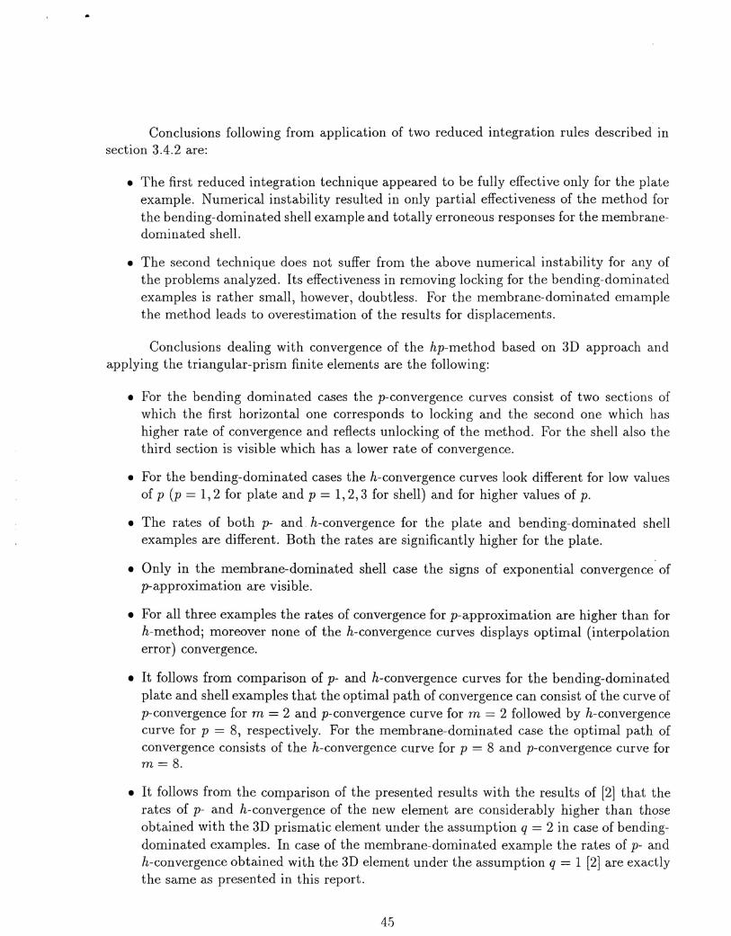
Conclusions following from application of two reduced integration rules described insection 3.4.2 are:

• The first reduced integration technique appeared to be fully effective only for the plateexample. Numerical instability resulted in only partial effectiveness of the method forthe bending-dominated shell example and totally erroneous responses for the membrane-dominated shell.

• The second technique does not suffer from the above numerical instability for any ofthe problems analyzed. Its effectiveness in removing locking for the bending-dominatedexamples is rather small, however, doubtless. For the membrane-dominated emamplethe method leads to overestimation of the results for displacements.

Conclusions dealing with convergence of the hp-method based on 3D approach andapplying the triangular-prism finite elements are the following:

• For the bending dominated cases the p-convergence curves consist of two sections ofwhich the first horizontal one corresponds to locking and the second one which hashigher rate of convergence and reflects unlocking of the method. For the shell also thethird section is visible which has a lower rate of convergence.

• For the bending-dominated cases the h-convergence curves look different for low valuesof p (p = 1,2 for plate and p = 1,2,3 for shell) and for higher values of p.

• The rates of both p- and h-convergence for the plate and bending-dominated shellexamples are different. Both the rates are significantly higher for the plate.

• Only in the membrane-dominated shell case the signs of exponential convergence ofp-approximation are visible.

• For all three examples the rates of convergence for p-approximation are higher than forh-methodj moreover none of the h-convergence curves displays optimal (interpolationerror) convergence.

• It follows from comparison of p- and h-convergence curves for the bending-dominatedplate and shell examples that the optimal path of convergence can consist of the curve ofp-convergence for m = 2 and p-convergence curve for m = 2 followed by h-convergencecurve for p = 8, respectively. For the membrane-dominated case the optimal path ofconvergence consists of the h-convergence curve for p = 8 and p-convergence curve form=8.

• It follows from the comparison of the presented results with the results of [2] that therates of p- and h-convergence of the new element are considerably higher than thoseobtained with the 3D prismatic element under the assumption q = 2 in case of bending-dominated examples. In case of the membrane-dominated example the rates of p- andh-convergence obtained with the 3D element under the assumption q = 1 [2]are exactlythe same as presented in this report.

4.5

As the strict criteria for applicability of the triangular-prism hp finite element (includ-ing locking and instability) in the thin limit (tja = 0.33%) for the plate, bending-dominatedshell and membrane-dominated shell cases are: p ~ 4, m ~ 2; p ~ 5, m ~ 2; p ~ 1, m ~ 6,respectively, then one can establish the following practical criteria for unconditional applica-bility of the element to any type of plate or shell problem in the thin limit (tja = 0.33%):p ~ 5, m ~ 6. This criteria can be relaxed for thicker plates or shells and must be tightenedfor thiner ones. Note, however, that for a large number of practical problems acceptableresults can be obtained for much lower values of p and m than those predicted above.

The hp-approximation based on 3D approach seems to work well for a wide selectionof plate and shell problems and for practically important range of thicknesses (0.1% or more).

46

References

[1] L. Demkowicz, J. T. Oden K., W. Rachowicz, O. Hardy. Towards a universal hp adaptivefinite element strategy, Part 1. Constrained approximation and data structure. CompoMeths Appl. Mech. Engng, 77, 79-112 (1989).

[2] G. Zboinski, L. Demkowicz. Application of the 3D hpq Adaptive Finite Element for Plateand Shell Analysis. TICOM Report 94-13. The Texas Institute for Computational andApplied Mathematics.

[3] L. Demkowicz, W. Rachowicz, K. Banas, J. Kucwaj. 2D hp Adaptive Package (2DhpAP).Report No. 1/1992 . Cracow University of Technology. Section of Applied Mathematics.Cracow 1992.

[4] L. Demkowicz, K. Banas: 3D hp Adaptive Package. Report No. 2/1993. Cracow Univer-sity of Technology. Section of Applied Mathematics. Cracow 1993.

[5] P. G. Ciarlet. Plates and Junctions in Elastic Multi-structures. Springer-Verlag, Masson.Berlin, Paris 1990.

[6] G. Zboinski. Application of a new thick shell finite element for analysis of long turbineblades. In: Proc. 17th International Seminar on Modal Analysis, Leuven (Belgium) 1992,977-993.

[7] O. C. Zienkiewicz, R. L. Taylor. The Finite Element Method, V. 2. McGraw-Hill BookCompany, London 1991.

[8] G. Zboinski, J. A. Kubiak. Application of the thick shell and transition elements foranalysis of the long turbine blades: Part I - An algorithm. In: Latest Advances in SteamTurbine Design, Blading, Repairs, Condition Assessment, and Condenser Interaction.Pwr-7, ASME, New York 1989, 23-30.

[9] L.Demkowicz, A. Bajer, K.Banas. Geometrical Modeling Package. TICOM Report 92-06.The Texas Institute for Computational Mechanics. The University of Texas at Austin.Austin 1992.

[10] S. Timoshenko, S. Woinowsky-Krieger. Theory of Plates and Shells. McGraw-HilL NewYork 1959.

[11] Y. Leino, J. Pitkaranta. On the membrane locking of h-p finite elements in cylindricalshell problem. Int. J. Num. Meths Engng, 37, 1053-1070 (1994).

[12] D. A. Dunavant. High degree efficient symmetrical Gaussian quadrature rules for thetriangle. Int. J. Num. Meths Engng, 21, 1129-1148 (1985).

[13] M. Bernadou, J. M. Boisserie. The Finite Element Method in Thin Shell Theory: Appli-catin to Arch Dam Simulations. Birkhauser. Boston-Basel-Stuttgart 1982.

47

,..

[14] J. Pitkaranta. The problem of membrane locking in finite element analysis of cylindricalshells. Numer. Math., 61, 523-542 (1992).

AQ

an adaptive 3d-based hp finite element for plate and shell

Documents