HAL Id: hal-01194811https://hal.inria.fr/hal-01194811

Submitted on 7 Sep 2015

HAL is a multi-disciplinary open accessarchive for the deposit and dissemination of sci-entific research documents, whether they are pub-lished or not. The documents may come fromteaching and research institutions in France orabroad, or from public or private research centers.

L’archive ouverte pluridisciplinaire HAL, estdestinée au dépôt et à la diffusion de documentsscientifiques de niveau recherche, publiés ou non,émanant des établissements d’enseignement et derecherche français ou étrangers, des laboratoirespublics ou privés.

A Comparative Analysis of Attitude Estimation forPedestrian Navigation with Smartphones

Thibaud Michel, Hassen Fourati, Pierre Genevès, Nabil Layaïda

To cite this version:Thibaud Michel, Hassen Fourati, Pierre Genevès, Nabil Layaïda. A Comparative Analysis of AttitudeEstimation for Pedestrian Navigation with Smartphones. Indoor Positioning and Indoor Navigation,Oct 2015, Banff, Canada. pp.10, 10.1109/IPIN.2015.7346767. hal-01194811

A Comparative Analysis of Attitude Estimation forPedestrian Navigation with Smartphones

Thibaud Michel∗†, Hassen Fourati†, Pierre Geneves∗, Nabil Layaıda∗∗Univ. Grenoble Alpes, LIG, CNRS, Inria, Grenoble, France†Univ. Grenoble Alpes, GIPSA-Lab, F38000 Grenoble, France

CNRS, GIPSA-Lab, F-38000 Grenoble, FranceInria

Abstract—We investigate the precision of attitude estimationsolutions in the context of Pedestrian Dead-Reckoning (PDR)with commodity smartphones and inertial/magnetic sensors. Wepropose a concise comparison and analysis of a number of attitudefiltering methods in this setting. We conduct an experimentalstudy with a precise ground truth obtained with a motion capturesystem. We precisely quantify the error in attitude estimationobtained with each filter which combines a 3-axis accelerometer,a 3-axis magnetometer and a 3-axis gyroscope measurements.We discuss the obtained results and analyse advantages andlimitations of current technology for further PDR research.

Keywords—Attitude Estimation, Sensor Fusion, Inertial andMagnetic Sensors, Kalman Filter and Observer, Smartphone, Pedes-trian Dead Reckoning.

I. INTRODUCTION

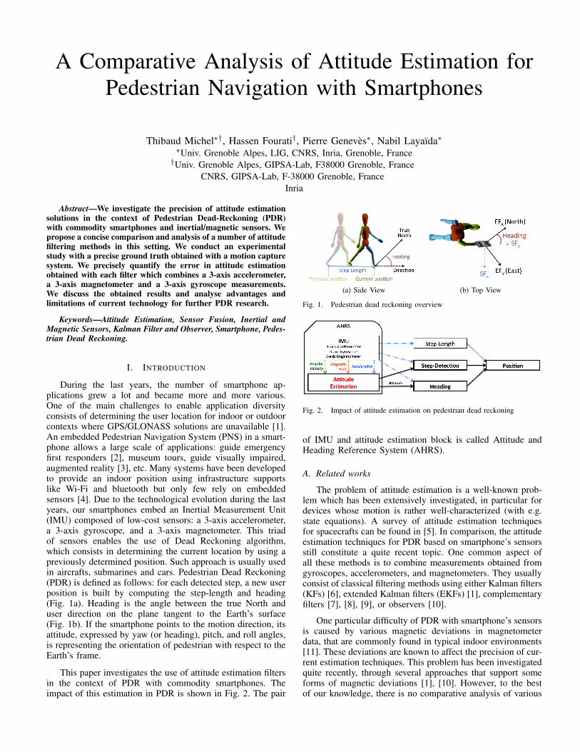
During the last years, the number of smartphone ap-plications grew a lot and became more and more various.One of the main challenges to enable application diversityconsists of determining the user location for indoor or outdoorcontexts where GPS/GLONASS solutions are unavailable [1].An embedded Pedestrian Navigation System (PNS) in a smart-phone allows a large scale of applications: guide emergencyfirst responders [2], museum tours, guide visually impaired,augmented reality [3], etc. Many systems have been developedto provide an indoor position using infrastructure supportslike Wi-Fi and bluetooth but only few rely on embeddedsensors [4]. Due to the technological evolution during the lastyears, our smartphones embed an Inertial Measurement Unit(IMU) composed of low-cost sensors: a 3-axis accelerometer,a 3-axis gyroscope, and a 3-axis magnetometer. This triadof sensors enables the use of Dead Reckoning algorithm,which consists in determining the current location by using apreviously determined position. Such approach is usually usedin aircrafts, submarines and cars. Pedestrian Dead Reckoning(PDR) is defined as follows: for each detected step, a new userposition is built by computing the step-length and heading(Fig. 1a). Heading is the angle between the true North anduser direction on the plane tangent to the Earth’s surface(Fig. 1b). If the smartphone points to the motion direction, itsattitude, expressed by yaw (or heading), pitch, and roll angles,is representing the orientation of pedestrian with respect to theEarth’s frame.

This paper investigates the use of attitude estimation filtersin the context of PDR with commodity smartphones. Theimpact of this estimation in PDR is shown in Fig. 2. The pair

(a) Side View (b) Top View

Fig. 1. Pedestrian dead reckoning overview

Fig. 2. Impact of attitude estimation on pedestrian dead reckoning

of IMU and attitude estimation block is called Attitude andHeading Reference System (AHRS).

A. Related works

The problem of attitude estimation is a well-known prob-lem which has been extensively investigated, in particular fordevices whose motion is rather well-characterized (with e.g.state equations). A survey of attitude estimation techniquesfor spacecrafts can be found in [5]. In comparison, the attitudeestimation techniques for PDR based on smartphone’s sensorsstill constitute a quite recent topic. One common aspect ofall these methods is to combine measurements obtained fromgyroscopes, accelerometers, and magnetometers. They usuallyconsist of classical filtering methods using either Kalman filters(KFs) [6], extended Kalman filters (EKFs) [1], complementaryfilters [7], [8], [9], or observers [10].

One particular difficulty of PDR with smartphone’s sensorsis caused by various magnetic deviations in magnetometerdata, that are commonly found in typical indoor environments[11]. These deviations are known to affect the precision of cur-rent estimation techniques. This problem has been investigatedquite recently, through several approaches that support someforms of magnetic deviations [1], [10]. However, to the bestof our knowledge, there is no comparative analysis of various

estimation filters in the setting of PDR with smartphone’ssensors. Authors typically evaluate their algorithms on theirown ground truth, and still unrelated to others. As a result, itis very hard to grasp the advantages and limitations of eachtechnique in our context.

B. Contributions

We propose a comparative analysis of recent attitudeestimation filters using smartphone’s sensors. We providean experimental setup with a precise ground truth obtainedthrough a motion capture system. We precisely quantify theattitude estimation error obtained with each technique. We payattention at reproducibility of results1. We analyze and discussthe results we have obtained.

C. Outline

The rest of the paper is organized as follows. In SectionII some useful notations, definitions and analysis for attitudeestimation are given. In Section III, we present six mainalgorithms for attitude estimation and we discuss some keypoints of these algorithms. In Section IV we describe theexperimental tests methodology, we report on the results ofattitude estimation that we have obtained with each algorithm,and we discuss the results before concluding the paper inSection V.

II. BACKGROUND FOR ATTITUDE ESTIMATION

A. Attitude representation

The smartphone attitude in PN is determinedwhen the axis orientation of the Smartphone FrameSF (SFx, SFy, SFz) is specified with respect to theEarth Frame EF (EFx, EFy, EFz) (see Fig. 3).

Fig. 3. The Smartphone-Frame SF (dashed line) and Earth-Frame EF (solidline).

The SFx-axis is horizontal and points to the right, the SFy-axis is vertical and points up and the SFz-axis points towardsthe outside of the front face of the screen. The EFy-axis pointsto the North. The EFz-axis points to the sky perpendicular tothe reference ellipsoid and the EFx-axis completes the right-handed coordinate system, pointing East (ENU : East, North,Down). An other convention is often used by aerial Vehiclescalled NED for North, East and Down.

Based on the literature, the attitude can be expressedwith three main different mathematical representations [12].Euler angles (roll, pitch, yaw (or heading)), rotation matrix orquaternion.

1Benchmarks can be reproduced using datasets on our website: http://tyrex.inria.fr/mobile/benchmarks-attitude

A unit-norm quaternion, which defines the rotation betweenEF and SF , is defined as:

q = SEq =

[q0−→q

]= [q0 q1 q2 q3]

T ∈ R4, (1)

where q0 and −→q being the scalar and the vector parts of thequaternion, respectively. We invite the reader to refer to [13]for more details about quaternion algebra.

Euler angles representation is composed of three mainrotations: a rotation ϕ around the x-axis (roll angle), a rotationθ around the y-axis (pitch angle) and a rotation ψ around thez-axis (yaw angle). More details about Euler angles proprietiescan be found in [14].

Rotation matrix for attitude estimation is a 3x3 matrixdefining three unit vectors yielding a total of 9 parameters.

Each one of these representations has some disadvan-tages, Euler angles have the well known gimbal-lock problem[14], rotation matrix contains 9 elements to be determinedand quaternion is less human understandable. Nevertheless,quaternion avoids the singularity problem involved in Eulerangles and is featured with simple computation cost andis easy to be operated for a large number of applications,especially in the case of smartphone environment. In SectionIV, the implemented algorithms under MATLAB are using thequaternion algebra [13]. A simple mathematical transformationbetween quaternion and Euler angles can be found in [14].

B. Sensors measurements and calibration

The sensors configuration of a smartphone is composed ofa triad of MEMS (Micro-Electro-Mechanical Systems) sensorsconsisting of a 3-axis gyroscope, a 3-axis accelerometer anda 3-axis magnetometer. The outputs of these low-cost sensorsare not perfect and suffer from several problems: noise, bias,scale factor, axis misalignment, axis non-orthogonality andlocal temperature. In the following, we will analyze the Allanvariance [15] on each sensor embedded in the smartphone(Google Nexus 5) to provide an accurate models. The Allanvariance analysis and results are similar to those proposed inother works [1], [16]. Let consider Sv as a 3x1 vector in theSmartphone frame and Ev as a 3x1 vector in the Earth frame.

1) Gyroscope: The 3-axis gyroscope measures the an-gular velocity of the smartphone in rad.s−1: Sω =[Sωx

SωySωz

]T. An Allan variance study [15] is applied

to the gyroscope signal. The results are shown in Fig. 4and three main noises are identified: an Angular RandomWalk (ARW) given by the − 1

2 slope part, a Bias Instability(BI) given by the 0 slope curve part and a Rate RandomWalk (RRW) given by the + 1

2 slope part. The widely usedcontinuous time model for a gyroscope can be written suchas:

Sω = Sωr + Sωb + Sωn, (2)

where

Sω is the angular rate measured by the gyroscope.Sωr is the true angular rate.Sωb is the gyroscope bias, where its derivative Sωb is

modeled by a random walk noise Sωb = Sωbn , its

standard deviation (BI) is noted Sσωbn. The gyroscope

bias leads after integration (see Eq. (7)) to an angulardrift, increasing linearly over time.

Sωn is the gyroscope white noise, its standard deviation(ARW) is noted Sσωn

.

10−2 10−1 100 101 102 103

10−2

10−1

Average time [sec]

AllanVariance

[deg/sec/√Hz] Axis x Axis y Axis z

Fig. 4. Allan variance of gyroscope signal.

Since the use of only gyroscope is not enough for attitudeestimation, other complementary sensors are used such asaccelerometers and magnetometers to compensate this drift.The accelerometer allows the correction of the pitch and rollangles whereas the magnetometer improves the yaw angle.So, how to pertinently combine inertial and magnetic sensormeasurements, is the key question to be solved when we arefacing to an attitude estimation problem.

2) Accelerometer: The 3-axis accelerometer measures thesum of the gravity and external acceleration of the smartphonein m.s−2: Sa =

[Sax

SaySaz]T

. In the same way as thegyroscope, we used the Allan variance on the accelerometersignal. The results are shown in Fig. 5 and three main noisesare identified: a Velocity Random Walk (VRW) given by the− 1

2 slope part, a Bias Instability (BI) given by the 0 slope curvepart and a Correlated Noise (CN) given by the oscillations(mostly on x-axis and z-axis). The continuous time model foraccelerometer can be written such as:

Sa = Sar + Sab + San, (3)

whereSa is the sum of the gravity and external acceleration of

the body measured by the accelerometer.Sar is the true sum of the gravity and external acceleration

of the body.Sab is the accelerometer bias, where its derivative S ab is

modeled by a Gauss-Markov noise: S ab = βSab+Sabn ,

the standard deviation of Sabn (BI) is noted Sσabn .San is the accelerometer white noise, its standard deviation

(VRW) is noted Sσan .

A uncalibrated accelerometer in a static phase providesa magnitude of acceleration close to g. In [17], the authorsprovide an accelerometer calibration algorithm based on a min-imum of 7 static phases. This calibration allows to remove thebias and misalignment by normalizing the acceleration vectorin multiple smartphone orientations. Finally the accelerationmagnitude is close to g.

10−2 10−1 100 101 102 103

10−1

100

Average time [sec]

AllanVariance

[mg/sec/√Hz] Axis x Axis y Axis z

Fig. 5. Allan variance of accelerometer signal.

3) Magnetometer: The 3-axis magnetometer measures themagnetic field of the smartphone in micro-tesla (µT ): Sm =[Smx

SmySmz

]T. The Earth’s magnetic field can be

modeled by a dipole and follows basic laws of magnetic fields.At any location, the Earth’s magnetic field can be representedby a three-dimensional vector and its intensity varies from25µT to 65µT . The National Geospatial-Intelligence Agency(NGA) and the United Kingdoms Defence Geographic Centre(DGC) provide a World Magnetic Model (WMM) [18] every5-years as shown in Fig. 6. Declination is used to know theangle between the Magnetic North and Geographic North,while inclination and intensity are used to build the referencevector.

Fig. 6. Earth’s magnetic field representation

The Allan variance is used on magnetometer signal andthe results are shown in Fig. 7 where three main noises areidentified: an Angle Random Walk (ARW) given by the − 1

2slope part, a Bias Instability (BI) given by the 0 slope curvepart and a Correlated Noise (CN) given by the oscillations.The continuous time model for magnetometer can be writtensuch as:

Sm = Smr + Smb + Smn, (4)

where

Sm is the magnetic field measured by the magnetometer.Smr is the true magnetic field.Smb is the magnetometer bias, where its derivative Smb is

modeled by a Gauss-Markov noise: Smb = βSmb +Smbn , the standard deviation of Smbn (BI) is notedSσmbn

.

Smn is the magnetometer white noise, its standard deviation(ARW) is noted Sσmn

.

10−2 10−1 100 101 102 103

10−1

100

Average time [sec]

AllanVariance

[µT/sec/√Hz] Axis x Axis y Axis z

Fig. 7. Allan variance of magnetometer signal.

Unfortunately, the magnetometer do not measure only theEarth’s magnetic field. Most of the time in indoor environ-ments, we are in presence of magnetic dipoles which perturbthe measure of Earth’s magnetic field. These perturbationscan be caused by electromagnetic devices (speakers, magnets),manmade structures (walls, floors) or other ferromagnetic ob-jects like belts, keys... For example, a speaker of a smartphonehas a field of about 2000µT (30 times more than the Earth’smagnetic field). A study in [11] categorizes the environmen-tal characteristics with respect to the magnetic deviations.Magnetic perturbations are categorized in two groups: hardand soft iron distortions. Hard iron distortions are causedby ferromagnetic materials in the smartphone frame SF (e.g.speaker for a smartphone). Soft iron distortions are causedby objects that produce a magnetic field (buildings walls,machines...) in the Earth frame EF. In a context free frommagnetic interferences, hard and soft iron distortions can becorrected at the same time by normalizing the magnetic fieldvector in a multiple smartphone orientations [19], [20].

III. ATTITUDE ESTIMATION ALGORITHMS OVERVIEW

For more clarity to the reader, we present in this section theoverall design of attitude estimation filters we need to compare.The selected filters [1], [6], [7], [8], [9], [10] from the literaturehave been designed for different applications and based onKalman filter, complementary filter and observer theories.

A. Filters design

The six algorithms are presented with a common notationson quaternion and sensors readings as described in Section IIand also below:

v = [vx vy vz]T is used for the estimated vector v,

kAcc, kGyr, kMag are the weight that are used to most trusta sensor that another,

qe, ωe are the quaternion and angular rate errors,∆t is the time difference between 2 epochs.

In order to estimate q, all presented algorithms use tworeference vectors Ea and Em.

In a perfect case (free of noise), the relation between Ea andSa is described as following:

Saq = q−1 ⊗ Eaq ⊗ q, (5)

where

⊗ is the quaternion multiplication [13].Saq is the quaternion form of Sa, which can be written such

as: Saq =[0 Sax

SaySaz]T

.Eaq is the quaternion form of Ea (such as Saq). In static

cases, Ea = [0 0 g]T where g is the acceleration due

to the gravity at the Earth’s surface (g ≈ 9.8 m.s−2).

In a perfect case (free of noise and magnetic deviation), therelation between Em and Sm is described as following:

Smq = q−1 ⊗ Emq ⊗ q, (6)

where

Smq is the quaternion form of Sm, which can be written suchas: Smq =

[0 Smx

SmySmz

]T.

Emq is the quaternion form of Em. In the absence of magneticdeviations, Em can be calculated by using the WMM[18].

The well-known kinematic equation of rigid body which isdefined from angular velocity measurements from a gyroscopeto describe the variation of the attitude in term of quaternioncan be written such as:

q =1

2q ⊗ Sωq, (7)

where Sωq is the quaternion form of Sω.

Algorithm 1 - Mahony et al. [7]Explicit Complementary Filter

S aq,t = q−1t−1 ⊗ Eaq,t ⊗ qt−1Smq,t = q−1t−1 ⊗ Emq,t ⊗ qt−1

Sωmes,t =[Sat × S at

]+[Smt × Smt

]S ˙ωb,t = −kiSωmes,tSωr,q,t = Sωq,t −

[0 Sωb,t

]+[0 kp

Sωmes,t]

kp and ki are proportional and integral adjustable gains (see Eq. (7)).

˙qt =1

2qt−1 ⊗ Sωr,q,t

Principles : This filter is an Explicit Complementary Filterdesigned for aerial vehicles. The algorithm calculates theerror by cross multiplying the measured and estimated vectors(acceleration and magnetic field), then this error allows tocorrect the gyroscope bias.

Algorithm 2 - Madgwick et al. [8]Gradient Descent based Orientation Filter

E hq,t = qt−1 ⊗ Smq,t ⊗ q−1t−1Emq,t =

[0 0

√E h2x,t + E h2y,t

E hz,t

]T

Ft =

[q−1t−1 ⊗ Eaq,t ⊗ qt−1 − Saq,tq−1t−1 ⊗ Emq,t ⊗ qt−1 − Smq,t

]qe,t = JTt Ft, where Jt is the Jacobian matrix of Ft (see [8])

Sωe,t = 2qt−1 ⊗ qe,tS ˙ωb,t = Sωe,tSωt = Sωt − ζSωb,t, where ζ is the integral gain.

˙qt =1

2qt−1 ⊗ Sωq,t − β

qe,t‖qe,t‖

β is the divergence rate of qt expressed as the magnitudeof a quaternion derivative corresponding to the gyroscopemeasurement error.

Principles : This filter is a Gradient Descent (GD) basedalgorithm designed for pedestrian navigation. The quaternionerror from the GD algorithm provides also a gyro driftcompensation.

Algorithm 3 - Fourati [9]Complementary Filter Algorithm

S aq,t = q−1t−1 ⊗ Eaq,t ⊗ qt−1Smq,t = q−1t−1 ⊗ Emq,t ⊗ qt−1

X = −2[[S at×] [

Smt×]]T , where:[

v×]

=

[0 −vz vyvz 0 −vx−vy vx 0

]K = [XTX + λI3×3]−1XT , with λ = 10−5

qe,t =

1

K

[Sat − S atSmt − Smt

]˙qt =

1

2qt−1 ⊗ Sωq,t ⊗ βqe,t

Principles : This filter is a mix between a GD algorithmand the quadratic approach of Marquardt designed forfoot-mounted devices. In this algorithm, there is nogyroscope drift compensation and only one adjustablegain is used. From author recommendations, we choseto put β = 5 when

∥∥Sa∥∥ − g < 0.03 and β = 0.5 for

others cases. Em used by Fourati is defined as follows:Em = [0 cos(inc) −sin(inc)]

T expressed in ENUcoordinates where inc is the inclination at the smartphonelocation defined by WMM [18].

Algorithm 4 - Martin et al. [10]Invariant Nonlinear Observers

Sc = [Sa× Sm] Ec = [Ea× Em]Sd = [Sc× Sa] Ed = [Ec× Ea]

Et =

[EAt

ECt

EDt

]=

Eaq − 1asqt−1 ⊗ Saq,t ⊗ q−1t−1

Ecq − 1csqt−1 ⊗ Scq,t ⊗ q−1t−1

Edq − 1as×cs qt−1 ⊗

Sdq,t ⊗ q−1t−1

LEt =kag2

Ea× EAt+

kc(Emyg)2

Ec× ECt+

kd(Emyg2)2

Ed× EDt

MEt = −kσLEt

NEt =kn

ka + kd

(kA〈EAt , EAt − Ea〉

g2+kD〈EDt , EDt − Ed〉

(Emyg2)2

)OEt =

koka + kd

(kC〈ECt

, ECt− Ec〉

(Emyg)2+kD〈EDt

, EDt− Ed〉

(Emyg2)2

)with ka, kc, kd, kσ, kn, ko > 0

˙qt =1

2qt−1 ⊗ (Sωq,t − Sωb,q,t) + LEt ⊗ qt−1

˙ωb = q−1t−1 ⊗MEt ⊗ qt−1˙as = as ×NEt˙cs = cs ×OEt

Principles : This filter is an observer with a new geometricalstructure from an engineering viewpoint. Authors introducenew measures: Sc is based on the product of Sa and Sm, Sdis the product of Sc and Sa. This approach does not require toknow all components of Em. Emy is the second componentof Em. An accelerometer, gyroscope and magnetometerbiases are estimated at every sample.

Algorithm 5 - Choukroun et al. [6]Linear Kalman Filter

Time update:

Ωt =

[0 −SωTtSωt −[Sωt

×]

]∆t

q−t = Φt × qTt−1, with Φt = exp(1

2Ωt)

Ξt =

[−−→qt

−[−→qt×] + q0t × I3×3

]Qf,t =

1

4ΞtQgΞ

Tt ∆t

P−t = ΩtPt−1ΩTt +Qf,tQg is the covariance matrix of state.

Measurement update:

sat =1

2(Sat + Ea) dat =

1

2(Sat − Ea)

smt =1

2(Smt + Em) dmt =

1

2(Smt − Em)

Hat =

[0 −dTatdat −[s×at ]

]Hmt

=

[0 −dTmt

dmt−[s×mt

]

]Ht =

[Hmt

Hat

]

E1t =

[−−→q

−t

−[−→q−t×] + q−0tI3×3

]

Rt =

[14 (E1tσmagE

T1t) + λI3 04×4

04×414 (E1t

SσanET1t) + λI3×3

]

Kt = P−t HTt (HtP

−t H

Tt + Rt)

−1

qt = q−t −KtHtq−t

Pt = (I4×4 −KtHt)P−t (I4×4 −KtHt) +KtRtK

Tt

Principles : This filter is the first one that provides alinearization of measurement equations. Then a Kalman Filteris applied and guarantees a global convergence.

Algorithm 6 - Renaudin et al. [1]EKF with opportunistic updates

State Vector:

x = [qt qωb,t abt ]T

Time update:

qω,t =

[cos( 1

2

∥∥Sωt∥∥∆t)

sin( 12

∥∥Sωt∥∥∆t)Sωt

‖Sωt‖

]qω,t = qω,t − qωb,t

qt = qt−1 ⊗ qω,t

xt = xt + δxt

δxt =

[C(qω,t) −M(qt) 0

0 I3×3 00 0 I3×3 − σabn ∆t

]δxt−1

+

[−M(qt) 0 00 I3×3∆t 00 0 I3×3∆t

][qωn

qωbn

an

]qωn

and qωbnare the qω noise and noise of bias.

Measurement update (only during QSF):

δzm,q,t = Emq,t − qt ⊗ Smq,t ⊗ q−1tδzm,t =

[h1(qt,

Em) 0 0]δx− h2(qt)mn

Smq,t = qω,t−1 ⊗ Smq,t−1 ⊗ q−1ω,t−1δzMARU,t = Smt − Smt

δzMARU,t =[0 −h3(qω,t,

Smt) 0]δx

+[I3×3 −h2(q−1ω,t)

] [ mnt

mnt−1

]

δza,q,t = Eaq − qt ⊗ (Saq,t − ab,t)⊗ q−1tδza,t =

[h1(qt,

Ea) 0 −h2(qt)]δxt − h2(qt)an

S aq,t = q−1ω,t−1 ⊗ (Saq,t−1 − ab,t−1)⊗ qω,t−1δzAGU,t = Sat − (S at + (I3×3 − σabn ∆t)abt−1

)

δzAGU,t =[0 −h3(qω,t,

S at − ab,t) I3×3 − (σabn ∆t+ h2(q−1ω,t))]δxt

+[I3×3 −h2(q−1ω,t)

] [ ant

ant−1

]

h1, h2, h3, C,M are defined in Renaudin’s paper [1].

Principles : This filter is an Extended Kalman Filter designedfor PDR algorithm. It does not use directly the gyroscopemodel (see Eq. (2)). The gyroscope signal is interpretedas a rotation between two successive epochs called qω . Anaccelerometer gradient update (AGU) is applied only duringQuasi-Static Field (QSF) periods. The same technique is usedfor magnetic angular rate update (MARU) during QSF. Apartfrom QSF periods, an integration on gyroscope measurementsis processed (see Eq. (7). The detector of QSF is not describedhere.

B. Discussions

All algorithms compared here share the same objective(finding an estimation of q) but rely on slightly differentmethods for this purpose: gradient descent, cross product error,Kalman filters, etc. From theory, there is no reason why onemethod would always perform better than the others, hencethe interest of our experimental analysis. We can howevercomment on a few assumptions used by several methods,which might be questionable when used in our context.

External acceleration. Algorithms used by Mahony, Madg-wick, Martin and Choukroun rely on a common assump-tion: external acceleration of the smartphone is negligi-ble. However, when used in this particular context ofsmartphone carried by a pedestrian, this assumption isquestionable. Specifically, the relation between Sa and Eagiven by Eq. (5) is true only if no external acceleration isapplied on the smartphone. Mahony, Madgwick, Martinand Choukroun consider external acceleration as negli-gible, but in some cases for a pedestrian, magnitude ofsmartphone external acceleration can rise up to 5m.s−2.Fourati takes it into account by adjusting gain according

to small or large accelerations. Renaudin’s approach isclose to Fourati’s one, a filter is applied only whenma(

∥∥Sa∥∥ − g) < λ where ma is a moving-average,otherwise an integration on gyroscope is computed (seeEq. (7)).

Magnetic deviations. Algorithms consider different tech-niques for dealing with magnetic deviations. Specifi-cally, different approaches are used for modelling Em.Choukroun and Fourati used a vector built from incli-nation described in Section II-B3, in other words theydo not consider magnetic deviations. Another approachconsiders small changes in magnetic field vector in theEF, it allows to use magnetic field vector of last sampleas reference. Madgwick, Mahony and Martin used thisapproach. Renaudin uses this last approach and combinesit with gyroscope integration (see Eq. (7)) when there arechanges in magnetic field vector. Among all algorithmscompared here, only Martin’s one prevents magneticdeviations from modifying pitch and roll values, only yawis impacted. We will verify experimentally this claim inthe next section.

Measurement models. Sensors are not considered by algo-rithms exactly as described in Section II-B. Table I showswhich noise and which bias are considered by algorithms.

TABLE I. SENSORS’ BIASES AND NOISES CONSIDERATION IN EACHALGORITHM

Gyroscope Accelerometer MagnetometerBias Noise Bias Noise Bias Noise

Mahony XMadgwick X

FouratiMartin X X X

Choukroun X2 X X XRenaudin X X X X X

The number of filters parameters can become a problembecause they are hard to estimate and depend on sensorsquality or sensors dynamics. Table II shows the number ofadjustable parameters in each algorithm excluding noiseand bias. Values of parameters used for Section IV aremostly extracted from authors’ papers:Mahony: kp=1 and ki=0.3.Madgwick: β = 0.08, ζ = 0.003 when time > 10s andζ=0 during the first ten seconds.

Fourati: It has no adjustable parameters since the gainis dynamic.

Martin: ka=0.7, kc=0.1, kd=0.01, kn=0.01, ko=0.01, kσ=0.05.

Choukroun: The only parameters are noises of sensors.Renaudin: Same parameters than Choukroun for noises

but for acceleration and magnetic field QSF detectors,thresholds are respectively λAcc = 3.92m.s−2 andλMag = 6µT .

TABLE II. NUMBER OF PARAMETERS OF EACH ALGORITHM

Mahony Madgwick Fourati Martin Choukroun Renaudin2 2 0 6 0 2

Globally, Kalman filters are easier to parametrize becausenoises values are only extracted from Allan variance.

2This bias has not been implemented in our version.

IV. COMPARATIVE ANALYSIS

A. Experimental context

Multiple experiences have been conducted with severalsmartphones (including LG Nexus 5, iPhone 5, Sony Xperia Z)and we obtained very similar results. A further study hasbeen made with LG Nexus 5, thanks to a homemade logapplication3. Internal sensors are really cheap and cost atmost 3e. The first one is a 6-axis InvenSense MPU6515accelerometer and gyroscope. The second one is a 3-axisAKM AK8963 magnetometer. InvenSense sensor can monitoractivity up to 200Hz while AKM one only to 60Hz. For thepurpose of aligning timestamps of magnetic field data withdata obtained from accelerometer and gyroscope, we used alinear extrapolation, in order to keep the focus on a real-timealgorithm, interpolation is unallowable here. We choose toalign data at 200Hz but similar results can be obtained untila sampling at 50Hz.

Tests have been made in a 10mx10m square motion lab4.In this room, we observed that the magnetic field is almosthomogeneous from a subplace to another (variations are lessthan 3µT : see Fig. 8), and with negligible variations over time.

Fig. 8. Heatmap of Magnetic Field of the Motion Lab.

Reference measurements have been made by a Qualisyssystem. This technology provides quaternions with a precisionof 0.5° of rotation. Our room is equipped with 20 Oquscameras connected to a server and Qualisys Tracker software.A 150Hz sampling is used. For the purpose of aligningtimestamps of our ground truth data with smartphone’s sensorsdata, we used slerp interpolation [21]. The motion trackerreference frame has been aligned with EF thanks to DGPSmeasures provided by room architects. A smartphone handlerwith infrared markers has been created with a 3D printer forthis study. Smartphone handler markers have been aligned withSF (Fig. 9).

Most of smartphones motion APIs (Android, iOS, Win-dows Phone) provide calibrated data. It is also possible to get

3https://github.com/sensbio/sensors-monitoring-android4See: http://kinovis.inrialpes.fr

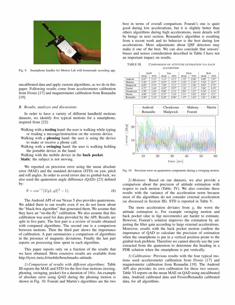
Fig. 9. Smartphone handler for Motion Lab with homemade recording app.

uncalibrated data and apply custom algorithms, as we do in thispaper. Following results come from accelerometer calibrationfrom Frosio [17] and magnetometer calibration from Renaudin[19].

B. Results, analyzes and discussions

In order to have a variety of different handheld motionsdatasets, we identify five typical motions for a smartphone,inspired from [22]:

Walking with a texting hand: the user is walking while typingor reading a message/instruction on the screens device.

Walking with a phoning hand: the user is using the deviceto make or receive a phone call.

Walking with a swinging hand: the user is walking holdingthe portable device in the hand.

Walking with the mobile device in the back pocket.Static: the subject is not moving.

We reported on precision error using the mean absoluteerror (MAE) and the standard deviation (STD) on yaw, pitchand roll angles. In order to avoid errors due to gimbal-lock, wealso used the quaternion angle difference (QAD) [23] definedby:

θ = cos−1(2〈q1, q2〉2 − 1). (8)

The Android API of our Nexus 5 also provides quaternions.We added them to our results even if we do not know aboutthe “black-box algorithm” that generated them. We assume thatthey have an “on-the-fly” calibration. We also assume that thiscalibration was used for data provided by the API. Results aresplit in five parts. The first part is a review of results obtainedwith compared algorithms. The second one is a comparisonbetween motions. Then the third part shows the importanceof calibration. A part summarizes a comparison of algorithmsin the presence of magnetic deviations. Finally the last partreports on processing time spent in each algorithm.

This paper reports only on a fraction of the results thatwe have obtained. More extensive results are available fromhttp://tyrex.inria.fr/mobile/benchmarks-attitude.

1) Comparison of results with different algorithms: TableIII reports the MAE and STD for the first four motions (texting,phoning, swinging, pocket) for a duration of 180s. An exampleof absolute error using QAD during the phoning motion isshown in Fig. 10. Fourati and Martin’s algorithms are the two

best in terms of overall comparison. Fourati’s one is quietgood during low accelerations, but it is slightly better thanothers algorithms during high accelerations, more details willbe brings in next section. Renaudin’s algorithm is resultingfrom a recent work and its behavior is the best during lowaccelerations. More adjustments about QSF detectors maymake it one of the best. We can also conclude that sensors’biases and noises consideration described in Table I have notan important impact on results.

TABLE III. COMPARISON OF ATTITUDE ESTIMATION VIA EACHALGORITHM.

QAD Yaw Pitch RollMAE STD MAE STD MAE STD MAE STD

Android 9.47° 5.15° 11.4° 15.2° 1.32° 0.98° 4.90° 7.07°Mahony 5.26° 4.57° 8.54° 12.9° 2.16° 2.34° 7.64° 10.7°Madgwick 6.05° 5.53° 7.58° 12.3° 2.33° 2.38° 9.03° 9.72°Fourati 4.72° 2.44° 6.92° 9.97° 1.24° 1.12° 5.66° 8.19°Choukroun 5.50° 2.44° 9.06° 12.4° 2.84° 3.21° 9.19° 12.4°Martin 4.80° 2.52° 8.37° 11.8° 2.11° 2.62° 8.83° 12.1°Renaudin 5.40° 2.14° 6.20° 6.96° 1.47° 1.62° 3.61° 4.48°

10 20 30 40 50 600

10

20

time [sec]

|error

|[deg

]

Android Choukroun Mahony MartinRenaudin Madgwick Fourati

Fig. 10. Precision error on quaternion components during a swinging motion.

2) Motions: Based on our datasets, we also provide acomparison about the precision of attitude estimation withrespect to each motion (Table. IV). We also correlate theseresults with the variance of the acceleration norm becausemost of the algorithms do not consider external acceleration(as discussed in Section III). STD is reported in Table V.

The more acceleration deviates from g, the worst theattitude estimation is. For example swinging motion andback pocket (due to hip movements) are harder to estimate.However, Fourati’s solution improves the estimation by ad-justing the filter gain according to large external accelerations.Moreover, results with the back pocket motion confirm theimportance of QAD to calculate the precision of estimationwhen the smartphone is put in a vertical position prone to thegimbal-lock problem. Therefore we cannot directly use the yawextracted from the quaternion to determine the heading in aPDR solution when the smartphone is put vertically.

3) Calibration: Previous results with the four typical mo-tions used accelerometer calibration from Frosio [17] andmagnetometer calibration from Renaudin [19]. The AndroidAPI also provides its own calibration for these two sensors.Table VI reports on the mean MAE on QAD using uncalibrateddata, Android calibrated data and Frosio/Renaudin calibrateddata, for all algorithms.

TABLE IV. COMPARISON OF ATTITUDE ESTIMATION ACCORDING TOTYPICAL MOTIONS.

QAD Yaw Pitch RollMAE STD MAE STD MAE STD MAE STD

Texting 3.88° 3.16° 2.91° 4.18° 0.99° 1.10° 1.40° 1.69°Phoning 4.24° 2.59° 2.84° 3.32° 1.42° 1.56° 2.45° 2.43°Pocket 6.05° 3.38° 21.5° 32.2° 1.65° 1.81° 22.4° 31.4°Swinging 7.50° 3.96° 3.85° 4.62° 4.06° 4.40° 3.09° 3.60°

TABLE V. STD OF ACCELERATION NORM IN THE FOUR MOTIONS INm.s−2 .

Texting Phoning Swinging Back pocket0.902 0.779 1.890 1.741

Uncalibrated data are unusable for attitude estimation algo-rithms. This is due to the fact that the internal speaker is closeto IMU (∼ 2cm) inside the smartphone. In a context free frommagnetic deviations, the mean of uncalibrated magnetic fieldmagnitude is about 350µT . This bias can easily be removedwith a calibration of hard iron deviations (same frame). Themagnetometer calibration given by Android API is enoughto have a good attitude estimation in most cases. Since thiscalibration is a “black-box” and the system calibrates on thefly, sometimes there is unwanted behavior (like in our phoningdataset where MAE = 20°), while Renaudin’s calibrationgives a MAE less than 4°. In our datasets, Renaudin’s cal-ibration improves the quality of attitude estimation by 4.5°compared to Android’s one. This improvement is significant.Finally, adding the Frosio calibration improves the globalprecision by 0.8°, event if this calibration is often tedious torealize.

TABLE VI. COMPARISON OF ATTITUDE ESTIMATION ACCORDING TOCALIBRATION.

Uncalibrated Android calib. Renaud. calib.Renaud. andFrosio calib.

MAE 92.64° 10.53° 6.05° 5.27°STD 41.13° 6.41° 3.58° 3.50°

4) Magnetic deviation: During the static phase we choseto test the algorithm resiliency to magnetic deviations on yaw,pitch and roll components. We used 6 small magnets and putthem close to the smartphone at 19sec and then removed themat 25sec. The magnetometer reported a magnitude of 250µTduring the period instead of 45µT for a free space (see Fig.11).

In the static phase, after a certain convergence period,all algorithms provides a stable but different estimation ofattitude. In order to discard these differences from our errormeasurements, we first substract the mean attitude estimationfor each dataset. Figs. 12, 13, 14 report the behaviors of the sixalgorithms during the magnetic deviation on QAD, yaw, pitchand roll. Scores on MAE and STD are shown in Table VII.

The only algorithms that are not impacted (or very little) bythe magnetic deviation during this static phase are Renaudin’sand Android ones. For Renaudin’s algorithm, this is thanks tothe detection of a high variation in the norm of the magneticfield, which is then used to discard magnetometer values intheir Kalman Filter [1]. Martin’s technique with the crossproduct of acceleration and magnetic field allows to avoid thedistortions on pitch and roll. Convergence of Fourati’s filter ismuch faster than with other algorithms (convergence delay isless than 1s after the magnet is removed). Moreover the pitch

and roll angles are not as significantly impacted as with theother approaches.

15 20 25 30 35 40 45 500

100

200

with magnet

time [sec]

|error

|[deg

]

Fig. 11. Magnitude of magnetic field using a magnet.

TABLE VII. COMPARISON OF ATTITUDE ESTIMATION UNDERMAGNETIC DEVIATION PROVIDED BY EACH ALGORITHM.

QAD Yaw Pitch RollMAE STD MAE STD MAE STD MAE STD

Android 0.01° 0.01° 0.03° 0.01° 0.02° 0.01° 0.06° 0.03°Mahony 17.1° 30.3° 17.2° 30.3° 0.39° 0.61° 0.56° 1.18°Madgwick 22.0° 24.8° 22.0° 24.8° 0.44° 0.65° 1.37° 2.06°Fourati 14.6° 27.6° 14.7° 27.6° 0.03° 0.05° 0.15° 0.23°Choukroun 14.2° 14.9° 14.3° 15.0° 0.36° 0.63° 1.29° 2.23°Martin 20.2° 26.2° 20.1° 26.2° 0.01° 0.01° 0.02° 0.03°Renaudin 0.55° 0.25° 0.48° 0.25° 0.01° 0.01° 0.03° 0.03°

15 20 25 30 35 40 45 500

50

100 with magnet

time [sec]

|error

|[deg

]

Android Choukroun Mahony MartinRenaudin Madgwick Fourati

Fig. 12. Precision error on yaw component with a magnet distortion.

15 20 25 30 35 40 45 500

1

2

3with magnet

time [sec]

|error

|[deg

]

Android Choukroun Mahony MartinRenaudin Madgwick Fourati

Fig. 13. Precision error on pitch component with a magnet distortion.

15 20 25 30 35 40 45 500

2

4

6

8 with magnet

time [sec]

|error

|[deg

]Android Choukroun Mahony MartinRenaudin Madgwick Fourati

Fig. 14. Precision error on roll component with a magnet distortion.

5) Processing time: Since the device is a smartphone andbattery saving is crucial, processing time matters. Table VIIIreports the number of quaternions generated per second usingMatlab. Computationally, the Madgwick filter outperforms theothers. The second line of the Table thus indicates the ratioof the time spent in each algorithm relative to the fastest(Madgwick).

TABLE VIII. PROCESSING TIME ON QUATERNION GENERATION(QUAT/SEC)

Mahony Madgwick Fourati Choukroun MartinQuaternion gen./sec 2762 4052 2559 2148 1257Relative to the best 0.68 1 0.63 0.53 0.31

Overall, in our setting, the two most suited algorithmsare the Martin’s observer and the complementary filter fromFourati. The first one is a bit more robust to magnetic devia-tions thanks to the cross product of acceleration and magneticfield but its precision is limited for high accelerations. In thissituation, the simple dynamic gain from Fourati’s algorithmshows good results. Other solutions like Madgwick one’s mightalso be especially interesting when the battery life is a priority.Some of the best ideas like Renaudin’s QSF or dynamicgains from Fourati will be the subject of our future researchestowards improved algorithms.

V. CONCLUSIONS

One major difficulty in PDR algorithms resides in preciseattitude estimation in the presence of magnetic deviations.Several techniques have been developed in the literature fordifferent scenarios. We provided an experimental setup with aprecise ground truth obtained through a motion capture system.We precisely quantified the attitude estimation error obtainedwith each technique. We analyzed and discussed the resultsthat we have obtained.

VI. ACKNOWLEDGMENTS

This work has been partially supported by the LabExPERSYVAL-Lab (ANR11-LABX-0025), EquipEx KINOVIS(ANR-11-EQPX-0024), EquipEx Robotex (ANR10-EQPX-44-01). We thank J.F. Cuniberto for the smartphone handler,J. Dumon and M. Heudre for the help in designing theexperimental platform and C. Combettes to provide Renaudin’sresults.

REFERENCES

[1] V. Renaudin and C. Combettes, “Magnetic, acceleration fields and gyro-scope quaternion (MAGYQ)-based attitude estimation with smartphonesensors for indoor pedestrian navigation,” Sensors, vol. 14, no. 12, pp.22 864–22 890, 2014.

[2] L. E. Miller, Indoor navigation for first responders: a feasibility study.Citeseer, 2006.

[3] M. Razafimahazo, N. Layaıda, P. Geneves, and T. Michel, “Mobileaugmented reality applications for smart cities,” ERCIM News 98,no. 98, pp. 45–46, Jul. 2014.

[4] R. Mautz, “Indoor positioning technologies,” Ph.D. dissertation, Habil-itationsschrift ETH Zurich, 2012.

[5] J. L. Crassidis, F. L. Markley, and Y. Cheng, “Survey of nonlinear atti-tude estimation methods,” Journal of Guidance, Control, and Dynamics,vol. 30, no. 1, pp. 12–28, 2007.

[6] D. Choukroun, I. Y. Bar-Itzhack, and Y. Oshman, “Novel quaternionkalman filter,” Aerospace and Electronic Systems, IEEE Transactionson, vol. 42, no. 1, pp. 174–190, 2006.

[7] R. Mahony, T. Hamel, and J.-M. Pflimlin, “Nonlinear complementaryfilters on the special orthogonal group,” Automatic Control, IEEETransactions on, vol. 53, no. 5, pp. 1203–1218, 2008.

[8] S. O. Madgwick, A. J. Harrison, and R. Vaidyanathan, “Estimation ofIMU and MARG orientation using a gradient descent algorithm,” inRehabilitation Robotics (ICORR), 2011 IEEE International Conferenceon. IEEE, 2011, pp. 1–7.

[9] H. Fourati, “Heterogeneous data fusion algorithm for pedestrian naviga-tion via foot-mounted inertial measurement unit and complementary fil-ter,” Instrumentation and Measurement, IEEE Transactions on, vol. 64,no. 1, pp. 221–229, Jan 2015.

[10] P. Martin and E. Salaun, “Design and implementation of a low-cost observer-based attitude and heading reference system,” ControlEngineering Practice, vol. 18, no. 7, pp. 712–722, 2010.

[11] M. H. Afzal, V. Renaudin, and G. Lachapelle, “Magnetic field basedheading estimation for pedestrian navigation environments,” in IndoorPositioning and Indoor Navigation (IPIN), 2011 International Confer-ence on. IEEE, 2011, pp. 1–10.

[12] D. Sachs, “Sensor fusion on android devices: A revolutionin motion processing,” [Video] https://www.youtube.com/watch?v=C7JQ7Rpwn2k, 2010, [Online; accessed 9-April-2015].

[13] J. B. Kuipers, Quaternions and rotation sequences, 1999, vol. 66.[14] J. Diebel, “Representing attitude: Euler angles, unit quaternions, and

rotation vectors,” Matrix, vol. 58, pp. 15–16, 2006.[15] X. Zhang, Y. Li, P. Mumford, and C. Rizos, “Allan variance analysis on

error characters of MEMS inertial sensors for an FPGA-based GPS/INSsystem,” in Proceedings of the International Symposium on GPS/GNNS,2008, pp. 127–133.

[16] H. Hou, Modeling inertial sensors errors using Allan variance. Uni-versity of Calgary, Department of Geomatics Engineering, 2004.

[17] I. Frosio, F. Pedersini, and N. A. Borghese, “Autocalibration ofMEMS accelerometers,” in Advanced Mechatronics and MEMS De-vices. Springer, 2013, pp. 53–88.

[18] U. (NGA) and the U.K.’s Defence Geographic Centre (DGC), “Theworld magnetic model,” http://www.ngdc.noaa.gov/geomag/WMM,2015, [Online; accessed 17-July-2015].

[19] V. Renaudin, M. H. Afzal, and G. Lachapelle, “New method formagnetometers based orientation estimation,” in Position Location andNavigation Symposium (PLANS), 2010 IEEE/ION. IEEE, 2010, pp.348–356.

[20] P. Bartz, “Magnetic compass calibration,” Oct. 13 1987, US Patent4,698,912.

[21] K. Shoemake, “Animating rotation with quaternion curves,” in ACMSIGGRAPH computer graphics, vol. 19, no. 3. ACM, 1985, pp. 245–254.

[22] V. Renaudin, M. Susi, and G. Lachapelle, “Step length estimation usinghandheld inertial sensors,” Sensors, vol. 12, no. 7, pp. 8507–8525, 2012.

[23] D. Q. Huynh, “Metrics for 3D rotations: Comparison and analysis,”Journal of Mathematical Imaging and Vision, vol. 35, no. 2, pp. 155–164, 2009.