Recursive Attitude Estimation in the Presence of Multi-rate and Multi-delayVector Measurements

Alireza Khosravian, Jochen Trumpf, Robert Mahony, Tarek Hamel

Abstract— This paper proposes an attitude estimationmethodology for the case where attitude sensors providediscrete-time samples of vector measurements at differentsample rates and with time delays. The proposed methodologyis based on a cascade combination of an output predictorand an attitude observer or filter. The predictor compensatesfor the effect of sampling and delays in vector measurementsand provides continuous-time predictions of outputs. Thesepredictions are then used in an observer or filter to estimatethe current attitude. The primary contribution of the paper isto exploit the underlying symmetry of the attitude kinematicsto design a recursive predictor that is computationally simpleand generic, in the sense that it can be combined with anyasymptotically stable observer or filter. We prove that thepredictor is able to reproduce the continuous time delay-freevector measurements. In a simulation example, we demonstrategood performance of the combined predictor-observer even inpresence of measurement noise and delay uncertainties.

I. INTRODUCTION

Attitude sensors mounted on a vehicle measure partialinformation about its attitude in the form of vector direc-tion measurements. The goal of an attitude estimator is tocompute the orientation of the vehicle by processing thosevector measurements. There is a large body of researchon both stochastic attitude estimation methods (such asextended Kalman filters [1], [2], unscented filters [3], etc.) aswell as deterministic attitude observers [4]–[16]. In satelliteattitude estimation applications, high accuracy sensors suchas star trackers or earth sensors provide measurements at lowsampling rates (0.5 to 10 Hz) [17]. In contrast, the onboardgyroscope can easily provide high bandwidth measurementsat kHz rates, potentially two orders of magnitude faster thanthe direction information is obtained. The image processinginside a star-tracker sensor can cause significant delays inthe order of tens of milliseconds, leading to the star-trackermeasurement being delayed with respect to the gyroscopemeasurements. Similar sampling and delay problems alsooccur in attitude estimation for aerial robots when visionbased sensors such as cameras and landmarks are employed.Also, in indoor flight environments, the attitude data fromdevices such as VICON or OptiTrack are delayed by the

A. Khosravian, J. Trumpf and R. Mahony are with the ResearchSchool of Engineering, Australian National University, ACT 2601, Aus-tralia (e-mail: alireza.khosravian@anu.edu.au; jochen.trumpf@anu.edu.au;robert.mahony@anu.edu.au).

T. Hamel is with I3S UNS-CNRS, France (e-mail: thamel@i3s.unice.fr).This work was partially supported by the Australian Research Council

through the ARC Discovery Project DP120100316 ”Geometric ObserverTheory for Mechanical Control Systems” and by the project ”SensoryControl of Aerial Robot” from French Agence Nationale de la Recherchethrough the ANR-ASTRID SCAR.

communication channel from these sensors to the onboardattitude estimation system of the vehicle.

Sampling and delays can negatively affect the stabilityand robustness of any observer or filter and degrade theirperformance if they are not compensated for properly [18]–[24]. Typical estimator design methodologies to tackle themeasurement sampling and delay problem are; estimatordesign with Lyapunov-Krasovskii modification, stochasticfiltering with Out-Of-Sequence Measurements (OOSM), andcompound observer-predictor design. The classical approachto tackle the sensor delay is to take an estimator that has thedesired performance for delay free measurements, and mod-ify its innovation term such that it compares each delayedmeasurement with its corresponding backward time-shiftedestimate. If the delay-free estimator has a Lyapunov stabilityproof, the stability analysis for the modified estimator can beundertaken using Lyapunov-Krasovskii functions [25], [26].Although these modified estimators are commonly used inpractice (see e.g. [27], [28]), they require complicated stabil-ity analyses and careful and conservative gain tuning, lead-ing to poor transient responses of the resulting estimators.Stochastic filtering with OOSM has been extensively studied[29]–[33], albeit most of this literature focuses on targettracking applications. Although OOSM filtering approachesare flexible, easily dealing with sampled and delayed dataas well as out-of-sequence measurements, they usually havesignificant memory and processing requirements that areunrealistic for most embedded observer design applications,except for linear system models where simpler OOSM filtersare available [20], [29]. For the specific problem of atti-tude estimation with sampled and delayed measurements,a modified extended Kalman filter with a novel real timeimplementation architecture is proposed in [34]. Despite itsgood performance in practice, this algorithm suffers frommajor drawbacks such as unclear convergence properties andhigh computational load due to the required propagationstages associated with sensor delay compensation. Combinedobserver-predictor design methods for nonlinear systems onRn have been developed in [19], [24], [35]. These methodstake observers that have the desired stability properties forcontinuous delay-free measurements and combine them withappropriate predictors that compensate for the effects ofsensor sampling and delays, such that the combined observer-predictor maintains the stability properties of the observer.The authors of this paper have recently proposed a cascadeobserver-predictor combination to handle sensor delay inthe attitude estimation problem [36]. Although the result-ing observer-predictor combination is stable, this method

requires continuous availability of sensor outputs and is notapplicable to the sampled measurement case. To the authors’knowledge, there is no attitude estimation methodology withstability proof available that considers sampled and delaymeasurements.

In this paper, we consider the attitude estimation prob-lem when sampled and delayed vector measurements areavailable. We propose a cascade combination of a predictorwith an attitude observer or filter in which the predictorcompensates for the effect of sampling as well as delaysin vector measurements and the filter or observer processesthe predicted outputs and estimates the attitude. Our designis based on the exact continuous time nonlinear attitudekinematics on the Lie group SO(3) without resorting toparameterization, linearization, or discretization. The maincontribution of the paper is to effectively employ the sym-metries of the attitude kinematics and vector measurementmodels to design a simple generic predictor that is inde-pendent of the choice of observer or filter. That is, ourproposed predictor can be combined with any observeror filter that has asymptotically stable estimation error inideal conditions (i.e. when it is fed with continuous timedelay-free vector measurements) and the predictor-observercombination maintains those stability properties in the non-ideal conditions (i.e. sampled and delayed measurements).The proposed predictor is recursive and requires only verysmall computational power, making it ideal for embeddedimplementation in real-world applications. We assume thatthe delay in each sensor measurement is known, that is werequire accurate time-stamping of data, however, this is theonly condition on the data. Given this assumption, the gaintuning process and the stability of the observer is independentof the size of the delay and valid even for time varyingdelays or OOSM measurements although we do not explicitlyconsider the latter in this paper. The proposed approachdirectly extends to the multi-rate measurement case withoutfurther modification. Via a simulation example, we show thatour predictor-observer method performs significantly betterthan Lyapunov-Krasowskii approach.

The structure of the paper is as follows. Background andproblem formulation is given in section II. The proposedpredictor-observer approach is described in section III wherethe main result of the paper is given by Theorem 1. Theperformance of our method is demonstrated via simulationsin section IV.

II. PROBLEM FORMULATION

Attitude determination sensors aim to measure physicalquantities that are usually continuous time objects by theirnature. Examples of these physical quantities are the lightintensity of stars or the Sun, respectively, sensed by starsensors or sun sensors, the Infra-Red reflection of the Earthsurface sensed by Earth sensors, or the magnetic field of theEarth sensed by magnetometers, all of which are continuoustime objects. In practice, however, attitude sensors are onlycapable of providing samples of those physical quantities atspecific sampling rates. Moreover, these samples are usually

delayed with respect to the measured physical quantities dueto various reasons such as slow response rates of the physicalparts of the sensors, internal processing time of sensors, andcommunication delays. In the following two subsections, wepresent a general discussion about modeling sampling anddelays in sensors. This discussion will then be applied to thespecific case of attitude sensors and vector measurements inSection II-C.

A. Physically inspired modeling of sampling and delays

We propose the model illustrated in Fig. 1 to includethe effect of sampling and delays on the output of sensors.This model is inspired by the physical process that takesplace in sensors during measuring a physical quantity. Thismodel consists of a zero-order-hold (ZOH) block that modelsthe effect of sampling and two delay blocks before andafter the ZOH that, respectively, model the pre-samplingand post-sampling delays. The pre-sampling delay on theleft side of Fig. 1 models ρi seconds of delay from whenthe physical quantity yi(t) occurs to when it is observedby the i-th sensor. We have yρi (t) = yi(t − ρi) for allt. In practice, this delay is usually due to the physicalproperties of the environment or the sensors. For instance,a star tracker requires that its imaging sensor is exposed tolight from stars for a specific amount of time so that it canproduce an image of the stars. This is known as exposuretime and can be as large as hundreds of milliseconds [37].The ZOH block in Fig. 1 takes the delayed signal andproduces a sample at time tki . This sample is latched atthe output of ZOH until the next sample is taken at timetki+1. Hence we have zρi (t) = yρi (tki) = yi(tki − ρi)for t ∈ [tki , tki+1). For clarity in presentation, we assumethat the sequence (tki)

∞ki=1 is an ordered monotonically

increasing sequence, i.e. tki−1 ≤ tki ≤ tki+1. However,this assumption is not necessary for our proposed methodand our method is also applicable to the case where themeasurements are out-of-sequence, although the necessarymodifications to the notation are rather cumbersome. Fora star tracker, the sequence (tki)

∞ki=1 corresponds to the

specific times when the star tracker obtains an image of stars.This sampling frequency can be as low as only 0.5 Hz upto 10 Hz for practical star trackers. The post-sampling delayon the right side of Fig. 1 models σi seconds of delay fromwhen a sample of the physical variable becomes available tothe sensor to the time when the new output zi(t) becomesavailable to the user. Hence we have

zi(t) = zρi (t− σi) = yi(tki − ρi), t ∈ [tki + σi, tki+1 + σi)(1)

In practice, the post-sampling delay models the delay dueto the internal signal processing in the sensor or due to thecommunication delay for transmitting information from thesensor to the user. For a star tracker, the post-sampling delayis mainly due to the processing time associated with imageprocessing algorithms that analyze the images taken by thestar tracker to recognize stars in the image and associate eachrecognized star with its corresponding star in the on-board

𝑧1 𝑡 = 𝑦 (𝑡 − 𝜏𝑝𝑟)

𝑧2 𝑡 = 𝑦 𝑘𝑇𝑠 − 𝜏𝑝𝑟

𝑡 ∈ [𝑘𝑇𝑠 , 𝑘 + 1 𝑇𝑠)

𝑧 𝑡 = 𝑦 𝑘𝑇𝑠 − 𝜏𝑝𝑟

𝑡 ∈ [𝑘𝑇𝑠 + 𝜏𝑝𝑜, 𝑘 + 1 𝑇𝑠 + 𝜏𝑝𝑜)

Sensor Model

𝑦: Ideal input to the sensor (i.e. variable to be measured)

𝑧1: Intermediate variable denoting the output of pre-sampling delay block.

𝑧2: Intermediate variable denoting the output of zero-order hold.

𝑧: Output of sensor (i.e. available measurement)

( )iy t ( )iy t ( )iz t

ikt

( )iz t

i i

Fig. 1. Modelling the effect of sampling and delays in attitude sensors

𝑧1 𝑡 = 𝑦 (𝑡 − 𝜏𝑝𝑟)

𝑧2 𝑡 = 𝑦 𝑘𝑇𝑠 − 𝜏𝑝𝑟

𝑡 ∈ [𝑘𝑇𝑠 , 𝑘 + 1 𝑇𝑠)

𝑧 𝑡 = 𝑦 𝑘𝑇𝑠 − 𝜏𝑝𝑟

𝑡 ∈ [𝑘𝑇𝑠 + 𝜏𝑝𝑜, 𝑘 + 1 𝑇𝑠 + 𝜏𝑝𝑜)

Sensor Model

𝑦: Ideal input to the sensor (i.e. variable to be measured)

𝑧1: Intermediate variable denoting the output of pre-sampling delay block.

𝑧2: Intermediate variable denoting the output of zero-order hold.

𝑧: Output of sensor (i.e. available measurement)

( )iy t ( )iy t ( )iz t

ikti

Fig. 2. Simple model that is input-to-output equivalent to Fig. 1

star catalog. The post-sampling delay can also model the lagdue to the communication delay from VICON or OptiTracksystems to the onboard attitude estimation system of flyingvehicles in indoor flight environments. It also can modelthe measurement delay associated with internal processingin GPS modules.

B. An input-to-output equivalent model

Although the model illustrated in Fig. 1 is suitable at themodeling stage to carefully describe the effect of samplingand various delays, it might not be convenient to be employedfor compensation of delays and sampling effects at the designstage. The main disadvantage of this model is that even if theuser knows the value of σi, the value of tki is only availablefrom the time tki + σi onwards. That is, the sensors usuallydo not inform the user when exactly they obtain samplesof measurements. Instead, they inform the user when theyfinish processing the samples and the processing result (i.e.the sensor output) is ready to be collected by the user. Thisis why we discuss a simpler model here which is input-to-output equivalent to Fig. 1, but is more convenient to use forcompensation of the effect of sampling and delays. Later onin this section, we discuss the condition under which thesetwo models are equivalent.

Assume that at time t′ki , ki = 1, 2, . . ., we receive themost recent output of the i-th sensor denoted by zi(t′ki). Weassume that this output is delayed τi seconds with respectto the measured physical quantity yi(t

′ki

). This output islatched until the next output arrives at t′ki+1. This procedureis equivalent to a cascade combination of a delay operatorand a ZOH, as sketched in Fig. 2. We have

zi(t) = zi(t′ki) = yi(t

′ki − τi), t ∈ [t′ki , t

′ki+1). (2)

Each sequence (t′ki)∞ki=1 is ordered monotonically increasing

(again, this assumption is not necessary for our method but itis imposed for clarity in presentation). The main differencecompared to the model discussed in Section II-A is that herethe sequence (t′ki) is known to the user and can be used forcompensating the effect of sampling and delays. It is obviousthat the outputs of Fig. 1 and Fig. 2 can be different ingeneral. However, simple calculations provided in AppendixA show that both models are input-to-output equivalent (i.e.the output zi(t) of both models are equal for all t when bothmodels measure the same physical quantity yi(t)) if and onlyif τi = ρi+σi and (t′ki)

∞ki=1 = (tki +σi)

∞ki=1. That is, when

both models are equivalent, the delay τi in Fig. 2 represents

the combination of the delays ρi and σi of Fig. 1 and thesampling sequence (t′ki)

∞ki=1 in Fig. 1 is equivalent to the

sequence of times by which the user receives the outputszi(t) of Fig. 2. Given a model in the form of Fig. 1, we arealways able to simplify that model to the form of Fig. 2 byproper choice of the delay and sampling sequence in Fig. 2.This in particular means that, as far as the input-to-outputcharacteristics of the sensors are concerned, there is no needto separately know the value of the pre-sampling and post-sampling delays. In fact, as we show in Section III, only theknowledge of the total delay τi between the physical valueyi(t) and the sensor output suffice to reproduce the physicalquantity yi(t) from the sampled and delayed sensor output.

C. Attitude kinematics and sensor models for vector mea-surements

Consider a rigid body with a body-fixed reference frameB and an inertial reference frame A. Denote the attitudematrix of the rigid body by R ∈ SO(3) that correspondsto the rotation from B to A. The rigid body attitudekinematics is given by

R(t) = R(t)Ω(t)×, R(0) = R0 (3)

where Ω is the angular velocity vector of B with respectto A expressed in B. The linear operator (.)× maps anyvector in R3 to its corresponding skew-symmetric matrix inso(3) such that (a)×b is equal to the cross product a× b forall a, b ∈ R3. We assume that delay-free measurements ofΩ(t) are available in continuous time. This is a reasonableassumption since in practice Ω(t) is measured at a highsampling rate using 3-axis gyros.

Ideal attitude sensors attached to the rigid body providepartial measurements of attitude in the form of vector mea-surements given by

yi(t) = R(t)>yi, i = 1, 2, . . . , n (4)

where yi ∈ S2 denotes the measured vector in B andyi ∈ S2 denotes the corresponding reference vector of yiin A. One can replace yi(t) from (4) into (1) and (2)to obtain attitude sensor models with sampling and delayscorresponding to Fig. 1 and Fig. 2, respectively.

The problem at hand is to design an estimation methodol-ogy that uses the continuous measurement of Ω(t) togetherwith the sampled and delayed vector measurements zi(t) toprovide continuous estimates of the attitude matrix R(t).

III. PREDICTOR-OBSERVER APPROACH

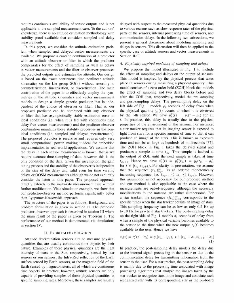
Due to the reasons discussed in Section II-B, we optto work with the simplified sensor model (2) to design analgorithm that compensates for the effects of sampling andboth pre and post-sampling delays and estimates the attitude.The approach that we propose here to tackle the problemformulated in Section II is illustrated in Fig. 3. We firstpropose a predictor that takes the sampled and delayed mea-surements zi(t) and provides continuous time predictions ofyi(t) denoted by ypi (t). The predictor relies on the knowledgeof Ω(t) in continuous time (or practically at high frequency)

Predictor

Observer

( ), 1,...,piy t i n

ˆ( )R t

( ), ( ), , 1,...,ii k it z t i n

( )t

Fig. 3. Illustration of the proposed predictor-observer approach (5)-(7)

and the total delay τi = ρi+σi to compensate for the effect ofsampling and delay in the outputs and to predict the outputssuch that ypi (t) = yi(t) for all t ≥ t′1i in noise-free conditions(i.e. when there is no measurement noise in zi(t′ki) or Ω(t)and the integration procedure within the predictor is alsoexact). The predicted outputs ypi (t), i = 1, . . . , n togetherwith the angular velocity measurement are then fed intoan observer to compute an estimate of attitude denoted byR(t). Our proposed predictor is generic in the sense thatit is independent of the employed observer algorithm, i.e.,the predictor can be coupled with any asymptotically stableattitude observer or filter to estimate the attitude.

Our proposed predictor takes the form

∆(t) = ∆(t)Ω(t)×, ∆(0) = ∆0, (5)

ypi (t) = ∆(t)>∆(t′ki − τi)zi(t), t ∈ [t′ki , t′ki+1), (6)

where ∆ ∈ SO(3) is the internal state of the predictor and∆0 ∈ SO(3) is an arbitrary initial condition. The trajectory∆(t) of the predictor dynamics (5) needs to be stored in abuffer for the previous t′ki+1 − t′ki + τi seconds in order tocompute the prediction ypi (t) (6) at each time.

The following theorem summarizes the properties of theproposed predictor.

Theorem 1: Consider the predictor (5)-(6) for the attitudedynamics (3) and the sensor measurements (2) with (4).The predicted output ypi (t) is equal to the ideal vectormeasurement yi(t) for all t > t1i and all choices of ∆0 ∈SO(3). Proof of Theorem 1 is given in Appendix B.

Even though the proposed predictor is independent of thechoice of observer, for the sake of concreteness, here wecouple the predictor with the following geometric attitudeobserver [10].

˙R(t) = R(t)

(Ω(t)− P (t)

n∑i=1

(Li(yi(t)− ypi (t))

)×yi(t)

)×,

(7)

with R(0) = R0 ∈ SO(3) and t ≥ maxi=1,...,n

t1i , where R(t)

is the estimate of R(t), yi(t) := R(t)>yi, and P (t) andLi, i = 1, . . . , n are positive definite gain matrices. Stability

of the pure observer (7) is shown in [38] for general positivedefinite gain matrices P (t) and Li, i = 1, . . . , n. These gainsare chosen to obtain the desired observer performance. Forinstance, P (t) can be recursively updated using Riccati dif-ferential equations as in extended Kalman filters [1], [2], or itcan be obtained using modified Riccati differential equationsas in geometric approximate minimum-energy filters [10].Choosing constant positive definite gain matrices simplifies(7) to the well-known geometric attitude observer proposedin [4], [7], [11], [39]. In any case, assuming that the observer(7) fed with the ideal vector measurements yi(t) rather thanthe predicted outputs ypi (t) (i.e. replacing ypi (t) with yi(t) in(7)) yields stable estimation error dynamics, then Theorem1 implies that the combined predictor-observer (5),(6), and(7) retains those stability properties of the observer for allchoices of ∆0 ∈ SO(3). In particular, if the constant gainobserver of [4] is employed as (7), then the estimated attitudeR(t) converges almost globally asymptotically and locallyexponentially to the true attitude R(t) for all choices of∆0 ∈ SO(3).

Note that in order to implement the proposed predictor-observer methodology, it is only required to implement onecopy of the predictor dynamics (5) and one copy of theobserver dynamics (7) even though we have several vectormeasurements zi(t), i = 1, . . . , n with possibly different de-lays τi and possibly different sampling sequences (t′ki)

∞ki=1.

Only a fixed duration buffer for the predictor state ∆(t) isneeded.

Remark 1: Our proposed method is also applicable tothe case where the delay τi is time-varying and out-of-sequence measurements do potentially occur. In this case, weshould replace the notation τi with τki (forming the sequence(τki)

∞ki=1) and each measurement delay τki should be known

to the user at time t′ki . Remark 2: Although the predictor-observer idea presented

in this paper focuses on the attitude kinematic system onSO(3), this idea can be generalized to kinematic systemson general Lie groups. For the very special case where theunderlying Lie group is Rn, the kinematic system is simplythe linear integrator x(t) = u(t) where x(t) ∈ Rn is thestate and u(t) ∈ Rn is the input. The output is given byy(t) = Cx(t) ∈ Rm where C ∈ Rm×n, and the sensorsprovide the delayed measurement z(t) = y(t− τ). It is easyto adapt the predictor proposed in this paper and obtain thefollowing simple predictor

δ(t) = u(t), (8)yp(t) = C(δ(t)− δ(t− τ)) + z(t). (9)

In this case, the predictor (8)-(9) corresponds to the well-known Smith predictor [40] originally designed for outputfeedback control of linear systems with delayed measure-ments. Note, however, that in the context of observers thispredictor does not seem to suffer from the Smith predictor’swell documented stability issues in the presence of delayuncertainty (see section IV).

IV. SIMULATION RESULTS

In this section, we provide a set of simulations to il-lustrate the performance of our proposed predictor-observermethodology. To generate the trajectory of R(t), we im-plement (3) with Ω(t) = [0; 0; 8] (deg/s) and the initialattitude R0 corresponding to the initial roll 14 (deg), pitch0 (deg), and yaw 0 (deg). We suppose that the attitudesensors provide the vector measurements corresponding tothe reference directions y1 = [1 0 0]> and y1 = [0 1 0]>.Although in practice the number of vector measurementscan be high and their directions are not necessarily pairwiseperpendicular (e.g. for star trackers), here we consider onlytwo vector measurements with perpendicular directions toavoid unnecessary discussions on gain tuning and focus onlyon the sampling and delay effects. To model z1(t) and z2(t),the ideal vector measurements y1(t) and y2(t) are obtainedby (4) and then fed to the block diagram of Fig. 1 withpre and post-sampling delays of ρ1 = ρ2 = 0.1 (s) andσ1 = σ2 = 0.3 (s), respectively, yielding a total delay ofτ1 = τ2 = 0.4 (s), and a sampling rate of 5 (Hz). Zeromean Gaussian noises with a standard deviation of 0.01are added to each axis of the vector measurements z1(t)and z2(t) which approximately add perturbations with thestandard deviation of 1 (deg) to the directions of z1(t) andz2(t). The angular velocity Ω(t) is sampled at 100 (Hz) andperturbed by an additive noise of 0.05 (deg/s) in each axis.

For the simulation, we combine the predictor (5)-(6) withthe geometric observer of [4]. This observer corresponds tochoosing scalar constant observer gains in (7) yielding

˙R(t) = R(t)

(Ω(t) + l1y

p1(t)×y1(t) + l2y

p2(t)×y2(t)

)×(10)

with yi(t) := R(t)>yi(t) and li > 0, i = 1, 2. We comparethe performance of this combined predictor-observer withan ad-hoc adaptation of the constant gain observer of [4]to the case of sampled and delayed vector measurements.The dynamics of the ad-hoc observer is given by ˙

Rad(t) =Rad(t)

(Ω(t) + α(t))× where Rad(t) is the estimate of R(t)

and α(t) is the innovation term. When the attitude sensorprovides the measured sample z1(t′k1) at time t = t′k1 , theinnovation term of the ad-hoc observer is inspired by theconstant gain observer as α(t′k1) = l1z1(t′k1)×Rad(t′k1 −τ1)>y1 with l1 > 0. This innovation term comparesthe newly received measurement z1(t′k1) with its estimateRad(t′k1 − τ1)>y1 in which the effect of the measurementdelay τ1 is considered1. Similarly, at time t = t′k2 whenthe measurement z2(t′k2) is delivered by attitude sensors, theinnovation term is α(t′k2) = l2z2(t′k2)×Rad(t′k2 − τ2)>y2with l2 > 0. If t′k2 happens to be equal to t′k1 for somepair (k1, k2), then the innovation term is simply the suml1z1(t′k1)×Rad(t′k1 − τ1)>y1 + l2z2(t′k2)×Rad(t′k2 − τ2)>y2.For the times where no sample of any vector measurementis available (i.e. for all t /∈ (tk1)∞ki=1 ∪ (tk2)∞ki=1), the

1Due to the consideration of the effect of delay in the innovation term,it can be thought of as a Lyapunov-Krasovskii term [25], [26], [35].

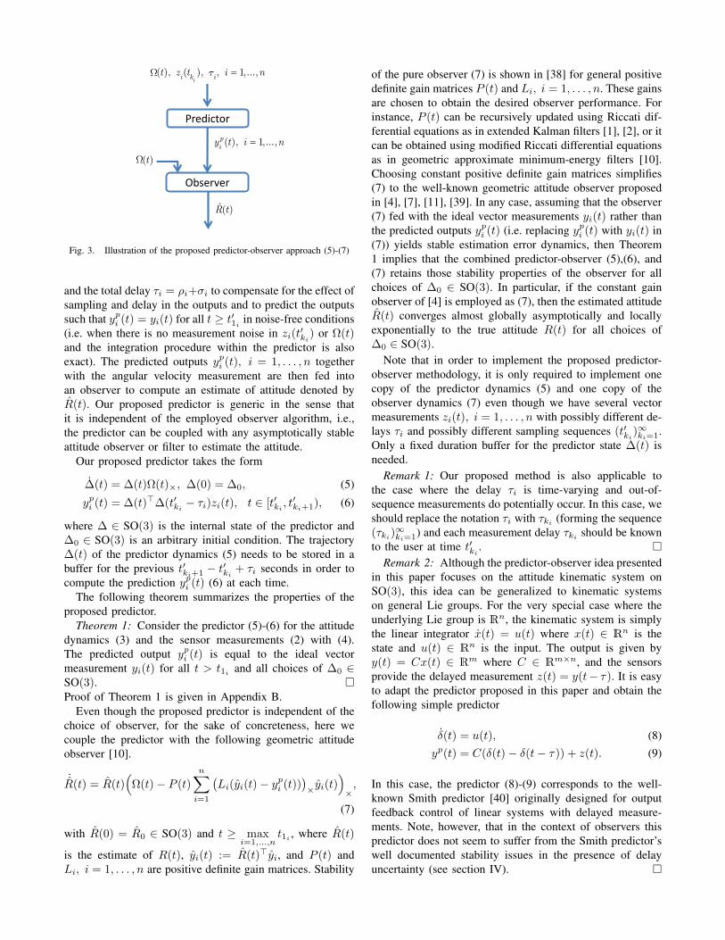
Fig. 4. Attitude estimation error of combined predictor-observer (5)-(7).The red plot is the enlarged steady state estimation error.

Fig. 5. Attitude estimation error of the ad-hoc observer. The red plot isthe enlarged steady state estimation error.

innovation term is zero which simplifies the observer to aforward integration of attitude kinematics. This innovationterm is mathematically formulated as follows.

α(t) =

l1z1(t′k1)×Rad(t′k1 − τ1)>y1, t = t′k1 6= t′k2l2z2(t′k2)×Rad(t′k2 − τ2)>y2, t = t′k2 6= t′k1∑2i=1 lizi(t

′ki

)×Rad(t′ki − τi)>yi, t = t′k1 = t′k2

0 t 6= t′ki

This ad-hoc method adaptation of observers is commonlyused in engineering applications to handle sensor samplingand delay effects (see e.g. [27], [28] for an EKF example).

The initial conditions of the combined predictor-observer(i.e. R(0.4) and ∆(0)) and the initial condition of thead-hoc observer (i.e. Rad(t), t ∈ [0, 0.4]) are set to theidentity matrix. The attitude estimation error of the combinedpredictor-observer is illustrated in Fig. 4, where the observergains are chosen as l1 = l2 = 0.5. In this figure, the errorθ is the angle of rotation in the angle-axis representationof the attitude estimate error R(t)R(t)> and is given byθ(t) = 180

π arccos(1− 0.5tr(I − R(t)R(t)>)). Note that theobserver trajectories are available after the first sample ofthe vector measurements have been provided by the attitudesensors. The red plot shows the steady state estimation errorwhich illustrates the good performance of our proposedmethod even with high sensor delay, low sampling rate,and high noise. Fig. 5 shows the estimation error θad(t) =180π arccos(1 − 0.5tr(I − Rad(t)R(t)>)) of the ad-hoc ob-

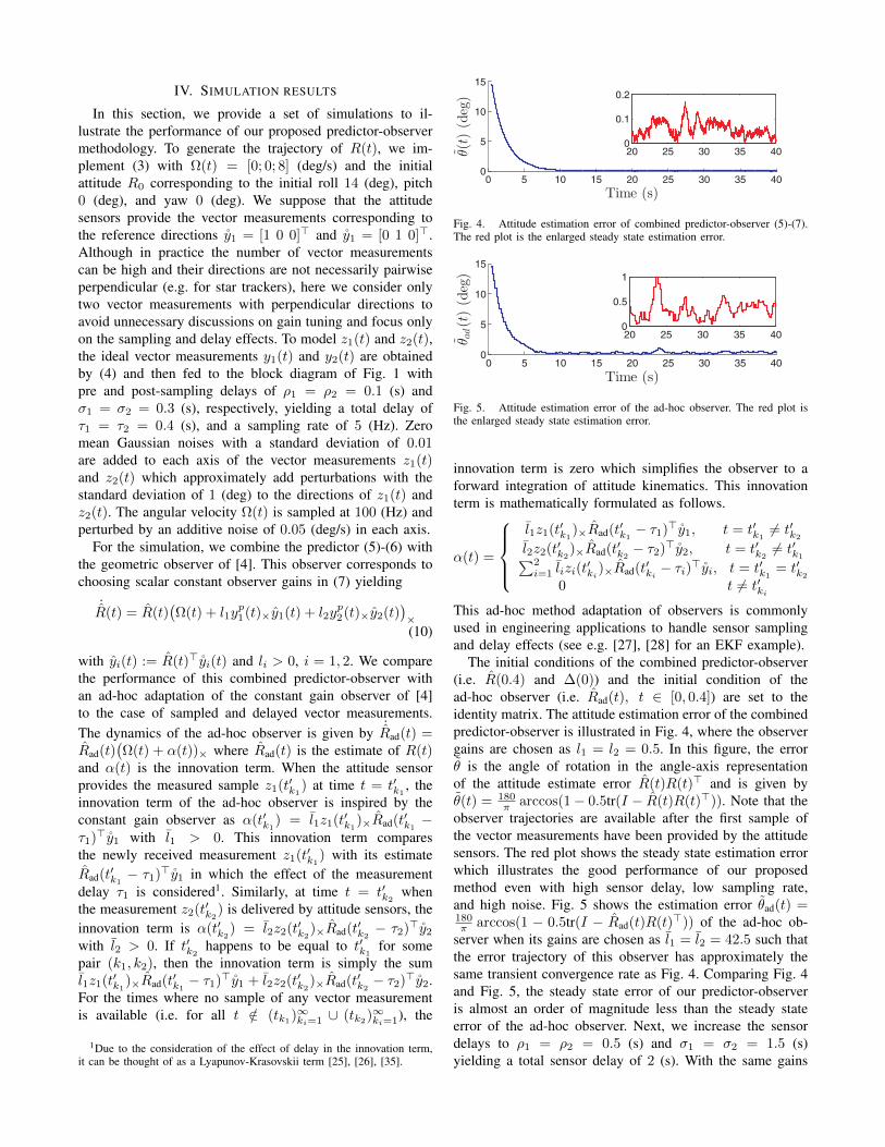
server when its gains are chosen as l1 = l2 = 42.5 such thatthe error trajectory of this observer has approximately thesame transient convergence rate as Fig. 4. Comparing Fig. 4and Fig. 5, the steady state error of our predictor-observeris almost an order of magnitude less than the steady stateerror of the ad-hoc observer. Next, we increase the sensordelays to ρ1 = ρ2 = 0.5 (s) and σ1 = σ2 = 1.5 (s)yielding a total sensor delay of 2 (s). With the same gains

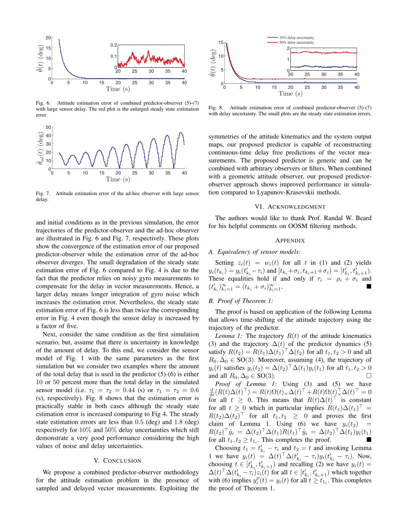
Fig. 6. Attitude estimation error of combined predictor-observer (5)-(7)with large sensor delay. The red plot is the enlarged steady state estimationerror.

Fig. 7. Attitude estimation error of the ad-hoc observer with large sensordelay.

and initial conditions as in the previous simulation, the errortrajectories of the predictor-observer and the ad-hoc observerare illustrated in Fig. 6 and Fig. 7, respectively. These plotsshow the convergence of the estimation error of our proposedpredictor-observer while the estimation error of the ad-hocobserver diverges. The small degradation of the steady stateestimation error of Fig. 6 compared to Fig. 4 is due to thefact that the predictor relies on noisy gyro measurements tocompensate for the delay in vector measurements. Hence, alarger delay means longer integration of gyro noise whichincreases the estimation error. Nevertheless, the steady stateestimation error of Fig. 6 is less than twice the correspondingerror in Fig. 4 even though the sensor delay is increased bya factor of five.

Next, consider the same condition as the first simulationscenario, but, assume that there is uncertainty in knowledgeof the amount of delay. To this end, we consider the sensormodel of Fig. 1 with the same parameters as the firstsimulation but we consider two examples where the amountof the total delay that is used in the predictor (5)-(6) is either10 or 50 percent more than the total delay in the simulatedsensor model (i.e. τ1 = τ2 = 0.44 (s) or τ1 = τ2 = 0.6(s), respectively). Fig. 8 shows that the estimation error ispractically stable in both cases although the steady stateestimation error is increased comparing to Fig 4. The steadystate estimation errors are less than 0.5 (deg) and 1.8 (deg)respectively for 10% and 50% delay uncertainties which stilldemonstrate a very good performance considering the highvalues of noise and delay uncertainties.

V. CONCLUSION

We propose a combined predictor-observer methodologyfor the attitude estimation problem in the presence ofsampled and delayed vector measurements. Exploiting the

Fig. 8. Attitude estimation error of combined predictor-observer (5)-(7)with delay uncertainty. The small plots are the steady state estimation errors.

symmetries of the attitude kinematics and the system outputmaps, our proposed predictor is capable of reconstructingcontinuous-time delay free predictions of the vector mea-surements. The proposed predictor is generic and can becombined with arbitrary observers or filters. When combinedwith a geometric attitude observer, our proposed predictor-observer approach shows improved performance in simula-tion compared to Lyapunov-Krasovskii methods.

VI. ACKNOWLEDGMENT

The authors would like to thank Prof. Randal W. Beardfor his helpful comments on OOSM filtering methods.

APPENDIX

A. Equivalency of sensor models:

Setting zi(t) = wi(t) for all t in (1) and (2) yieldsyi(tki) = yi(t

′ki−τi) and [tki +σi, tki+1+σi) = [t′ki , t

′ki+1).

These equalities hold if and only if τi = ρi + σi and(t′ki)

∞ki=1 = (tki + σi)

∞ki=1.

B. Proof of Theorem 1:

The proof is based on application of the following Lemmathat allows time-shifting of the attitude trajectory using thetrajectory of the predictor.

Lemma 1: The trajectory R(t) of the attitude kinematics(3) and the trajectory ∆(t) of the predictor dynamics (5)satisfy R(t2) = R(t1)∆(t1)>∆(t2) for all t1, t2 > 0 and allR0,∆0 ∈ SO(3). Moreover, assuming (4), the trajectory ofyi(t) satisfies yi(t2) = ∆(t2)>∆(t1)yi(t1) for all t1, t2 > 0and all R0,∆0 ∈ SO(3).

Proof of Lemma 1: Using (3) and (5) we haveddt (R(t)∆(t)>) = R(t)Ω(t)×∆(t)>+R(t)Ω(t)>×∆(t)> = 0for all t ≥ 0. This means that R(t)∆(t)> is constantfor all t ≥ 0 which in particular implies R(t1)∆(t1)> =R(t2)∆(t2)> for all t1, t2 ≥ 0 and proves the firstclaim of Lemma 1. Using (6) we have yi(t2) =R(t2)>yi = ∆(t2)>∆(t1)R(t1)>yi = ∆(t2)>∆(t1)yi(t1)for all t1, t2 ≥ t1i . This completes the proof.

Choosing t1 = t′ki − τi and t2 = t and invoking Lemma1 we have yi(t) = ∆(t)>∆(t′ki − τi)yi(t

′ki− τi). Now,

choosing t ∈ [t′ki , t′ki+1) and recalling (2) we have yi(t) =

∆(t)>∆(t′ki− τi)zi(t) for all t ∈ [t′ki , t′ki+1) which together

with (6) implies ypi (t) = yi(t) for all t ≥ t1i . This completesthe proof of Theorem 1.

REFERENCES

[1] F. L. Markley, “Attitude error representations for kalman filtering,”Journal of guidance, control, and dynamics, vol. 26, no. 2, pp. 311–317, 2003.

[2] E. J. Lefferts, F. L. Markley, and M. D. Shuster, “Kalman filteringfor spacecraft attitude estimation,” Journal of Guidance, Control, andDynamics, vol. 5, no. 5, pp. 417–429, 1982.

[3] J. L. Crassidis and F. L. Markley, “Unscented filtering for spacecraftattitude estimation,” Journal of guidance, control, and dynamics,vol. 26, no. 4, pp. 536–542, 2003.

[4] R. Mahony, T. Hamel, and J.M. Pflimlin, “Nonlinear complementaryfilters on the special orthogonal group,” IEEE Trans. Autom. Control,vol. 53, no. 5, pp. 1203–1218, 2008.

[5] H. F. Grip, T. I. Fossen, T. A. Johansen, and A. Saberi, “Globallyexponentially stable attitude and gyro bias estimation with applicationto GNSS/INS integration,” Automatica, vol. 51, pp. 158–166, 2015.

[6] J. Vasconcelos, C. Silvestre, and P. Oliveira, “A nonlinear observerfor rigid body attitude estimation using vector observations,” in Proc.IFAC World Congr., Korea, July 2008.

[7] S. Bonnabel, P. Martin, and P. Rouchon, “Symmetry-preserving ob-servers,” IEEE Trans. Autom. Control, vol. 53, no. 11, pp. 2514–2526,2008.

[8] A. Roberts and A. Tayebi, “On the attitude estimation of acceleratingrigid-bodies using GPS and IMU measurements,” in IEEE Conf.Decision and Control and European Control Conf. (CDC-ECC), 2011,pp. 8088–8093.

[9] M. Izadi and A. K. Sanyal, “Rigid body attitude estimation based onthe Lagrange–d’Alembert principle,” Automatica, vol. 50, no. 10, pp.2570–2577, 2014.

[10] M. Zamani, J. Trumpf, and R. Mahony, “Minimum-energy filtering forattitude estimation,” IEEE Transactions on Automatic Control, vol. 58,pp. 2917–2921, 2013.

[11] H. Rehbinder and B. K. Ghosh, “Pose estimation using line-baseddynamic vision and inertial sensors,” IEEE Trans. Automatic Control,vol. 48, no. 2, pp. 186–199, 2003.

[12] A. Khosravian and M. Namvar, “Globally exponential estimation ofsatellite attitude using a single vector measurement and gyro,” in Proc.49th IEEE Conf. Decision and Control, USA, Dec. 2010.

[13] A. Khosravian, J. Trumpf, R. Mahony, and C. Lageman, “Biasestimation for invariant systems on Lie groups with homogeneousoutputs,” in Proc. IEEE Conf. on Decision and Control, December2013.

[14] P. Martin and E. Salaun, “Design and implementation of a low-cost observer-based attitude and heading reference system,” ControlEngineering Practice, vol. 18, no. 7, pp. 712–722, 2010.

[15] M.-D. Hua, “Attitude estimation for accelerated vehicles usingGPS/INS measurements,” Control Engineering Practice, vol. 18, no. 7,pp. 723–732, 2010.

[16] M.-D. Hua, P. Martin, and T. Hamel, “Velocity-aided attitude esti-mation for accelerated rigid bodies,” arXiv preprint arXiv:1411.3953,2014.

[17] F. L. Markley and J. L. Crassidis, Fundamentals of Spacecraft AttitudeDetermination and Control. Springer, 2014.

[18] M. Arcak and D. Nesic, “A framework for nonlinear sampled-dataobserver design via approximate discrete-time models and emulation,”Automatica, vol. 40, no. 11, pp. 1931–1938, 2004.

[19] T. Ahmed-Ali, I. Karafyllis, and F. Lamnabhi-Lagarrigue, “Globalexponential sampled-data observers for nonlinear systems with delayedmeasurements,” Systems & Control Letters, vol. 62, no. 7, pp. 539–549, 2013.

[20] B. Khaleghi, A. Khamis, F. O. Karray, and S. N. Razavi, “Multisensordata fusion: A review of the state-of-the-art,” Information Fusion,vol. 14, no. 1, pp. 28–44, 2013.

[21] F. Deza, E. Busvelle, J. Gauthier, and D. Rakotopara, “High gainestimation for nonlinear systems,” Systems & control letters, vol. 18,no. 4, pp. 295–299, 1992.

[22] W. H. Heemels, A. R. Teel, N. van de Wouw, and D. Nesic, “Net-worked control systems with communication constraints: Tradeoffsbetween transmission intervals, delays and performance,” IEEE Trans.Automatic Control, vol. 55, no. 8, pp. 1781–1796, 2010.

[23] H. Hammouri, M. Nadri, and R. Mota, “Constant gain observer forcontinuous-discrete time uniformly observable systems,” in Proc. IEEEConf. Decision and Control, 2006, pp. 5406–5411.

[24] I. Karafyllis and C. Kravaris, “From continuous-time design tosampled-data design of observers,” IEEE Trans. Automatic Control,vol. 54, no. 9, pp. 2169–2174, 2009.

[25] T. Ahmed-Ali, E. Cherrier, and F. Lamnabhi-Lagarrigue, “Cascadehigh gain predictors for a class of nonlinear systems,” IEEE Trans.Automatic Control, vol. 57, no. 1, pp. 221–226, 2012.

[26] S. Bahrami and M. Namvar, “Delay compensation in global estimationof rigid-body attitude under biased velocity measurement,” in Proc.IEEE Conf. on Decision and Control, December 2014.

[27] P. Riseborough, (visited on September 2014). [Online]. Available:https://github.com/priseborough/InertialNav

[28] “APM: Navigation extended Kalman filter overview,”(visited on September 2014). [Online]. Available:http://copter.ardupilot.com/wiki/common-apm-navigation-extended-kalman-filter-overview/

[29] Y. Bar-Shalom, H. Chen, and M. Mallick, “One-step solution for themultistep out-of-sequence-measurement problem in tracking,” IEEETrans. Aerospace and Electronic Systems, vol. 40, no. 1, pp. 27–37,2004.

[30] M. Mallick, J. Krant, and Y. Bar-Shalom, “Multi-sensor multi-targettracking using out-of-sequence measurements,” in Proc. IEEE Inter-national Conf. Information Fusion, vol. 1, 2002, pp. 135–142.

[31] R. W. Beard, private communication, 2014.[32] K. Zhang, X. R. Li, and Y. Zhu, “Optimal update with out-of-sequence

measurements,” IEEE Trans. Signal Processing, vol. 53, no. 6, pp.1992–2004, 2005.

[33] Y. Bar-Shalom, “Update with out-of-sequence measurements in track-ing: exact solution,” IEEE Trans. Aerospace and Electronic Systems,vol. 38, no. 3, pp. 769–777, 2002.

[34] D. B. Kingston and R. W. Beard, “Real-time attitude and positionestimation for small UAVs using low-cost sensors,” in AIAA 3rdUnmanned Unlimited Technical Conference, Workshop and Exhibit,2004.

[35] A. Germani, C. Manes, and P. Pepe, “A new approach to stateobservation of nonlinear systems with delayed output,” IEEE Trans.Automatic Control, vol. 47, no. 1, pp. 96–101, 2002.

[36] A. Khosravian, J. Trumpf, R. Mahony, and T. Hamel, “Velocity aidedattitude estimation on SO(3) with sensor delay,” in Proc. IEEE Conf.on Decision and Control, December 2014, (accepted for publication).

[37] T. Sun, F. Xing, Z. You, and M. Wei, “Motion-blurred star acquisitionmethod of the star tracker under high dynamic conditions,” Opticsexpress, vol. 21, no. 17, pp. 20 096–20 110, 2013.

[38] A. Khosravian, J. Trumpf, R. Mahony, and C. Lageman, “Observersfor invariant systems on lie groups with biased input measurementsand homogeneous outputs,” Automatica, (to appear).

[39] J. Vasconcelos, C. Silvestre, and P. Oliveira, “A nonlinear observerfor rigid body attitude estimation using vector observations,” in Proc.IFAC World Congr., Korea, July 2008.

[40] O. J. Smith, “A controller to overcome dead time,” ISA Journal ofInstrument Society of America, vol. 6, no. 2, pp. 28–33, 1959.