a closer look at wave-function/density-functional hybrid
TRANSCRIPT

HAL Id: tel-01471720https://tel.archives-ouvertes.fr/tel-01471720
Submitted on 20 Feb 2017
HAL is a multi-disciplinary open accessarchive for the deposit and dissemination of sci-entific research documents, whether they are pub-lished or not. The documents may come fromteaching and research institutions in France orabroad, or from public or private research centers.
L’archive ouverte pluridisciplinaire HAL, estdestinée au dépôt et à la diffusion de documentsscientifiques de niveau recherche, publiés ou non,émanant des établissements d’enseignement et derecherche français ou étrangers, des laboratoirespublics ou privés.
A closer look at wave-function/density-functional hybridmethodsOdile Franck
To cite this version:Odile Franck. A closer look at wave-function/density-functional hybrid methods. Theoretical and/orphysical chemistry. Université Pierre et Marie Curie - Paris VI, 2016. English. NNT : 2016PA066303.tel-01471720

Universite Pierre et Marie Curie
Ecole Doctorale de Chimie Physique et de Chimie Analytique deParis Centre
These de doctoratDiscipline : Chimie Theorique
presentee par
Odile Franck
A closer look at wave-function/density-functional hybridmethods
dirigee par Julien Toulouse
Soutenue le 29 septembre 2016 devant le jury compose de :
M. Stephane Carniato UPMC presidentMme Paola Gori-Giorgi Vrije Universiteit Amsterdam rapporteurM. Trond Saue CNRS & Universite Paul Sabatier rapporteur
M. Janos Angyan CNRS & Universite de Loraine examinateurM. Emmanuel Fromager Universite de Strasbourg examinateurMme Eleonora Luppi UPMC co-encadrantM. Julien Toulouse UPMC directeur

Laboratoire de Chimie Theorique4, place Jussieu75 005 Paris
UPMCEcole Doctorale de Chimie Physiqueet de Chimie Analytique de Paris Centre4 place Jussieu75252 Paris Cedex 05

Acknowledgments
J’aimerais dans un premier temps remercier tous ceux qui ont rendu la realisation de cette
these possible : le Laboratoire de Chimie Theorique et son directeur Olivier Parisel qui m’ont
accueillie, l’Institut du Calcul et de la Simulation ainsi que le LABEX Calsimlab pour le fi-
nancement. J’aimerais aussi remercier Julien et Eleonora pour leur patience et leur disponibilite
pendant ces trois annees.
J’aimerais remercier Eric Cances ainsi que Gabriel Stoltz, Antoine Levitt et David Gontier
pour les echanges interessants, entre autre sur la convergence en base. J’aimerais aussi remercier
Irek Grabowski ainsi que Szymon Smiga et Adam Buksztel pour une collaboration interessante.
Enfin j’aimerais remercier Bastien pour son aide.
J’aimerais remercier les membres du jury de these qui ont accepte de juger mon manuscrit et
de participer a la soutenance; Paola Gori-Giorgi, Trond Saue, Stephane Carniato, Janos Angyan
et Emmanuel Fromager.
J’aimerais aussi remercier toutes les personnes qui ont partage a un moment ou a un autre
notre open space de travail ou les gouters etudiants du LCT : Stephanie, Elisa, Samira, Ines,
Etienne, Daniel, Aixiao, Olivier, Mohamed, Ozge, Eleonore, Emanuele, Sehr, Lea et tout parti-
culierement Roberto et Christophe pour leur bonne humeur. Les personnes du groupe de travail
de l’ICS Genevieve, Chantal, Lydie, Roman, Chiara, Silvia, Jeremy, Loıc, Louis.
J’aimerais remercier Marie-France pour le support informatique et pour le reste.
J’aimerais remercier toutes les personnes qui sont venues assister a la soutenance.
Enfin j’aimerais remercier les membres du Laboratoire de Chimie Quantique de Strasbourg
qui m’ont permis de me lancer dans cette belle aventure qu’est la recherche.
iii

iv

Contents
Introduction 1
1 Review of density-functional theory and hybrid methods 7
1.1 Schrodinger equation . . . . . . . . . . . . . . . . . . . . . . . . . . . . . . . . . . 7
1.2 Density-functional theory . . . . . . . . . . . . . . . . . . . . . . . . . . . . . . . 8
1.2.1 Hohenberg-Kohn theorems . . . . . . . . . . . . . . . . . . . . . . . . . . 8
1.2.2 Kohn-Sham approach . . . . . . . . . . . . . . . . . . . . . . . . . . . . . 10
1.2.3 Some approximated functionals . . . . . . . . . . . . . . . . . . . . . . . . 12
1.3 Range-separated hybrid approximations . . . . . . . . . . . . . . . . . . . . . . . 15
2 Basis convergence of range-separated density-functional theory 19
3 Self-consistent double-hybrid density-functional theory using the optimized-
effective-potential method 49
4 Study of the short-range exchange-correlation kernel 79
4.1 Introduction . . . . . . . . . . . . . . . . . . . . . . . . . . . . . . . . . . . . . . . 79
4.2 Review on time-dependent density-functional theory . . . . . . . . . . . . . . . . 80
4.2.1 Time-dependent Schrodinger equation for many-electron systems . . . . . 80
4.2.2 Time-dependent density-functional theory: the Kohn-Sham formalism . . 80
4.2.3 Linear-response . . . . . . . . . . . . . . . . . . . . . . . . . . . . . . . . . 81
4.2.4 Range-separated TDDFT . . . . . . . . . . . . . . . . . . . . . . . . . . . 82
4.3 Study of the short-range exchange kernel . . . . . . . . . . . . . . . . . . . . . . . 83
4.3.1 Range-separated time-dependent exact-exchange method . . . . . . . . . 83
4.3.2 Short-range exact-exchange kernel . . . . . . . . . . . . . . . . . . . . . . 86
4.4 Asymptotic expansion with respect to the range-separation parameter of the
short-range exchange kernel . . . . . . . . . . . . . . . . . . . . . . . . . . . . . . 88
4.4.1 Leading-order contribution . . . . . . . . . . . . . . . . . . . . . . . . . . 88
4.4.2 Next-order contribution . . . . . . . . . . . . . . . . . . . . . . . . . . . . 89
4.4.3 Examples of H2 and He . . . . . . . . . . . . . . . . . . . . . . . . . . . . 89
4.5 Study of the exact frequency-dependent correlation kernel . . . . . . . . . . . . . 92
v

vi CONTENTS
4.5.1 FCI of H2 in minimal basis set . . . . . . . . . . . . . . . . . . . . . . . . 92
4.5.2 Calculation of the linear-response function . . . . . . . . . . . . . . . . . . 93
4.5.3 Derivation of the exact short-range correlation kernel . . . . . . . . . . . . 94
4.5.4 Calculations on H2 in STO-3G basis . . . . . . . . . . . . . . . . . . . . . 98
4.6 Conclusion . . . . . . . . . . . . . . . . . . . . . . . . . . . . . . . . . . . . . . . 100
Conclusion 105
A Additional results for the basis-set convergence of the long-range correlation
energy 107
A.1 Convergence of the correlation energy including core electrons . . . . . . . . . . . 107
A.2 Extrapolation scheme . . . . . . . . . . . . . . . . . . . . . . . . . . . . . . . . . 108
B Derivation of the exact-exchange kernel 111
Resume en francais 121

Introduction
Early attempts of building a density-functional theory can be found in the work of Thomas
[1] and Fermi [2] in 1927. In their model the energy is expressed with respect to the density
with a simple expression for the kinetic energy based on the uniform electron gas and nuclear-
electron and electron-electron interactions are described classically. This model was extended
to the Thomas-Fermi-Dirac model by including an exchange energy formula for the uniform
electron gas introduced by Dirac [3] in 1930. Another early model was given by Slater [4] in
1951 who proposed an approximation to the non-local exchange in the Hartree-Fock method
that depends only on the local electron density. Density-functional theory as known today was
first introduced in 1964 by Hohenberg and Kohn [5] as an alternative to solving the Schrodinger
equation. Density-functional theory applied in the Kohn-Sham [6] scheme is an exact method if
the exact exchange-correlation density functional is known, unfortunately it is not and a major
topic of research is to define better and better approximated functionals. The first approximated
functional that was proposed and that was used as a starting point to further development is
based on an model system, an hypothetical uniform electron gas. In this approximation at each
point of an inhomogeneous system the local exchange-correlation energy per particle is taken as
the exchange-correlation energy per particle of the uniform electron gas of the same density. This
approximation is called the local-density approximation (LDA), the most known parametrization
was given by Vosko et al.[7]. Even if LDA is based on a simple approximation, realistic systems
being different from an uniform electron gas, it performs surprisingly good and can even be
comparable to or better in accuracy than Hartree-Fock, showing good accuracy for molecular
properties such as equilibrium structure but failing to describe energetical quantities such as
bonding energies with an overbinding tendency. An extension to improve the performance of
LDA is to take information from the gradient of the density to take into account the non-
homogeneity of the true electronic density which leads to a new family of approximations:
generalized-gradient approximations (GGAs). An example of such functional is given by B88
[8] for the exchange and LYP [9] for the correlation. A way to improve the performance of
GGAs is to take into account the Laplacian of the density and/or the kinetic energy density,
leading to a new family of approximations: meta-generalized-gradient approximations (meta-
GGAs). One of the most used meta-GGA approximation is TPSS defined by Tao et al.[10].
LDA, GGAs and meta-GGAs are often referred to as semilocal approximations because they
1

2 INTRODUCTION
only depend on the density at a point or on the derivatives of the density at this point (or
the derivatives of the orbitals for meta-GGAs). These semilocal approximations often give
an accurate description of short-range dynamical correlation but fails to describe long-range
or static correlation. These semilocal approximations present typically a self-interaction error
which tends to favor delocalization of the electrons and induces too low total energies.
A way to improve the performance of approximated functionals, in particular by reducing
the self-interaction error, is to combine density-functional theory with wave-function theory and
create hybrid approximations. Combining both theories can be done in different ways. One of
the simplest way of doing it is by doing a linear separation of the electron-electron Coulomb
interaction into two parts
1
r=
λ
r︸︷︷︸WFT
+(1− λ)
r︸ ︷︷ ︸DFT
,
the first term being treated with using wave-function theory (WFT) while the second term be-
ing treated with density-functional theory (DFT) and λ is the parameter of this hybridation.
A first realization of this was done in 1993 by Becke with the half-and-half combination [11]
(i.e. λ = 0.5) of Hartree-Fock exchange and a density-functional approximation. Most of the
time this fraction of Hartree-Fock exchange was too important and some error compensation
between exchange and correlation was lost. Later this hybrid scheme was extended using sev-
eral empirical coefficients with a smaller coefficient of Hartree-Fock exchange [12]. Common
hybrid approximations nowadays use a fraction λ ' 0.2 − 0.25 of Hartree-Fock exchange [13].
An extension of such hybrid approximations is achieved by introducing a fraction of correlation
energy calculated using second-order Møller-Plesset perturbation theory (MP2) and is known as
double-hybrid approximations. It was originally introduced by Grimme [14]. Double-hybrid ap-
proximations allow us to use a more important fraction of Hartree-Fock exchange (λ ' 0.5−0.7)
than for hybrid approximations without loosing too much the benefit of the error compensation
but the method fails to describe phenomena that cannot be treated with MP2, for example
static correlation. The fraction of correlation energy calculated with wave-function theory can
be treated using other approximations such as random-phase approximations [15]. To improve
the description of static correlation, density-functional theory can also be combined with the
multiconfiguration self-consistent-field (MCSCF) method [16].
Combining density-functional theory and wave-function theory can be done going beyond
the linear combination with the range-separated approach introduced by Savin [17] in 1996 by
decomposing the electron-electron Coulomb interaction into a long-range part and a short-range
part using the error function

3
1
r=
erf(µr)
r︸ ︷︷ ︸WFT
+1− erf(µr)
r︸ ︷︷ ︸DFT
,
where µ is a parameter controlling the range of the separation. The long-range interaction is
described using wave-function theory and the short-range interaction is described using density-
functional theory. A version limited to the range separation of the exchange, named long-range
correction scheme (LC), was proposed by Iikura et al.[18] by introducing long-range Hartree-
Fock exchange while short-range exchange and correlation are treated using density-functional
approximations. The range separation can also be done on the correlation, for example using
MP2 for the long-range correlation with long-range Hartree-Fock exchange and a short-range
exchange-correlation functional [19]. Such a decomposition can be performed using other meth-
ods to describe the long-range correlation such as random-phase approximations [20] or coupled-
cluster methods [21], which are well adapted to describe van der Waals dispersion interactions.
A multiconfigurational treatment of the long-range correlation can be used to improve the de-
scription of static correlation such as long-range MCSCF [22] or long-range density-matrix-
functional theory (DMFT) [23].
The density-functional theory formalism has been extended to describe excited states, with
linear-response time-dependent density-functional theory. The key quantity in this approxima-
tion is the exchange-correlation kernel. The spatial and frequency dependence of this kernel
needs to be approximated. The simplest approximation is the adiabatic semilocal approxi-
mation in which the kernel is local in time (i.e., independent of the frequency) and local in
space. This approximation gives reasonably good results for low-lying valence electronic exci-
tation energies of molecular systems but it fails to describe some phenomena such as multiple
excitations, charge-transfer excitation energies and Rydberg excitation energies. To overcome
these limitations, time-dependent density-functional theory has been extended to range separa-
tion. The decomposition of the exchange kernel into a long-range Hartree-Fock exchange kernel
and a short-range exchange kernel described by a density-functional approximation has first
been performed by Tawada et al.[24] and was able to correct some problems from the semilocal
approximation such as the description of Rydberg excitation energies and charge-transfer exci-
tation energies. The range-separated scheme can be extended by using a short-range correlation
kernel calculated with a density-functional approximation and using long-range linear-response
MCSCF [25] or long-range linear-response DMFT [26] approaches. The use of multiconfigura-
tional methods to describe the long-range response improves the description of static correlation
and it also allows one to calculate double excitations. The short-range correlation kernel can
also be combined with a long-range correlation kernel calculated using the many-body Green
function formalism [27] which gives us a frequency-dependent long-range correlation kernel.

4 INTRODUCTION
In this thesis we will investigate several aspects of hybrid methods combining wave-function
theory and density-functional theory. The first chapter will give a brief overview of density-
functional theory and these hybrid approaches.
In the second chapter the study is centered on the basis-set convergence of range-separated
hybrid methods. The basis-set convergence has been studied a lot for wave-function theory and
range-separated hybrid methods have been shown to converge faster, but the convergence rate
had not been explored yet. In this chapter we first studied the convergence in a partial-wave
expansion of the long-range wave function with respect to the maximal angular momentum. We
then studied the convergence of the long-range second-order Møller-Plesset correlation energy
with respect to the cardinal number of the Duning basis sets (cc-p(C)VXZ). The obtained results
allowed us to propose a three-point extrapolation scheme for the complete basis set energy of
range-separated hybrid density-functional theory.
The third chapter will be focused on double-hybrid density-functional methods combining
density-functional theory with second-order Møller-Plesset perturbation theory (MP2). These
methods give accurate results for thermochemical properties. Commonly the orbitals are eval-
uated without the MP2 term, which is added a posteriori. Recently Peverati and Head-Gordon
[28] proposed an orbital-optimized double-hybrid method where the orbitals are self-consistently
optimized in the presence of the MP2 correlation term. This orbital-optimized double-hybrid
method has shown an improvement in the spin-unrestricted calculations for symmetry breaking
and open-shell situations. In this study we will consider an alternative orbital-optimized double-
hybrid method based on the optimized-effective-potential (OEP) method that could bring ad-
vantages for calculations of excitation energy and response properties and a better description of
the LUMO orbital energy. We will compare the results for such an OEP double-hybrid method
to the standard double-hybrid method for the calculation of atomic and molecular properties
such as ionization potentials and electronic affinities.
In the fourth chapter we will consider range-separated linear-response time-dependent density-
functional theory and we will study the short-range exchange and correlation kernels. We
started by generalizing the exact-exchange kernel [29, 30] to range-separated time-dependent
density-functional theory. We then studied the behavior of the kernel with respect to the range-
separation parameter (µ) and we compared the behavior of the short-range exchange kernel
with the adiabatic LDA for He and H2. Finally we studied the frequency-dependent short-range
correlation kernel for a model system: H2 in a minimal basis set.
Finally in the last chapter we will give some general concluding remarks and outline.
BIBLIOGRAPHY 5
Bibliography
[1] L. H. Thomas. The Calculation of Atomic Fields. Proc. Camb. Phil. Soc. , 23:542, 1927.
[2] E. Fermi. Un Metodo Statistice per la Determinazionedi Alcune Proprieta dell’ Atomo.Rend. Accad. Lincei, 6:602, 1927.
[3] P. A. M. Dirac. Note on Exchange Phenomena in the Thomas Atom.Proc. Camb. Phil. Soc. , 26:376, 1930.
[4] J. C. Slater. A Simplification of the Hartree-Fock Method. Phys. Rev. , 81:385, 1951.
[5] P. Hohenberg and W. Kohn. Inhomogeneous Electron Gas. Phys. Rev. B, 136:864, 1964.
[6] W. Kohn and L. J. Sham. Self Consistent Equations Including Exchange and CorrelationEffects. Phys. Rev. A, 140:1133, 1965.
[7] S. J. Vosko, L. Wilk, and M. Nusair. Accurate Spin-Dependent Electron Liquid CorrelationEnergies for Local Spin Density Calculations: A Critical Analysis. Can. J. Phys., 58:1200,1980.
[8] A. D. Becke. Density-functional exchange-energy approximation with correct asymptoticbehavior. Phys. Rev. A, 38:3098, 1988.
[9] C. Lee, W. Yang, and R. G. Parr. Development of the Colle-Salvetti correlation-energyformula into a functional of the electron density. Phys. Rev. B, 37:785, 1988.
[10] J. Tao, J. P. Perdew, V. N. Staroverov, and G. E. Scuseria. Climbing the Density FunctionalLadder: Nonempirical Meta-Generalized Gradient Approximation Designed for Moleculesand Solids. Phys. Rev. Lett. , 91:146401, 2003.
[11] A. D. Becke. A new mixing of Hartree-Fock and local density-functional theories.J. Chem. Phys. , 98:1372, 1993.
[12] A. D. Becke. Density-functional thermochemistry. III. The role of exact exchange.J. Chem. Phys. , 98:5648, 1993.
[13] J. P. Perdew, M. Ernzerhof, and K. Burke. Rationale for mixing exact exchange withdensity functional approximations. J. Chem. Phys. , 105:9982, 1996.
[14] S. Grimme. Semiempirical hybrid density functional with perturbative second-order corre-lation. J. Chem. Phys. , 124:034108, 2006.
[15] A. Ruzsinszky, J. P. Perdew, and G. I. Csonka. The RPA Atomization Energy Puzzle.J. Chem. Theory Comput. , 6:127, 2010.
[16] K. Sharkas, A. Savin, H. J. Aa. Jensen, and J. Toulouse. A multiconfigurational hybriddensity-functional theory. J. Chem. Phys. , 137:044104, 2012.
[17] A. Savin. Recent Development and Applications in Modern Density Functional Theory. J.M. Seminario (Elsvier, Amsterdam), 1996.
[18] H. Iikura, T. Tsuneda, T. Yanai, and K. Hirao. A long-range correction scheme forgeneralized-gradient-approximation exchange functionals. J. Chem. Phys. , 115:3540, 2001.

6 BIBLIOGRAPHY
[19] A. Savin J. Toulouse J. G. Angyan, I. C. Gerber. Van der Waals forces in density functionaltheory: Perturbational long-range electron-interaction corrections. Phys. Rev. A, 72:012510,2005.
[20] J. Toulouse, I. C. Gerber, G. Jansen, A. Savin, and J. G. Angyan. Adiabatic-Connection Fluctuation-Dissipation Density-Functional Theory Based on Range Separa-tion. Phys. Rev. Lett. , 102:096404, 2009.
[21] E. Goll, H.-J. Werner, and H. Stoll. A short-range gradient-corrected density functionalin long-range coupled-cluster calculations for rare gas dimers. Phys. Chem. Chem. Phys. ,7:3917, 2005.
[22] E. Fromager, J. Toulouse, and H. J. A. Jensen. On the universality of the long-/short-rangeseparation in multiconfigurational density-functional theory. J. Chem. Phys. , 126:074111,2007.
[23] D. R. Rohr, J. Toulouse, and K. Pernal. Combining density-functional theory and density-matrix-functional theory. Phys. Rev. A, 82:052502, 2010.
[24] Y. Tawada, T. Tsuneda, S. Yanagisawa, and K. Hirao. A long-range-corrected time-dependent density functional theory. J. Chem. Phys. , 120:8425, 2004.
[25] E. Fromager, S. Knecht, and H. J. A. Jensen. Multi-configuration time-dependent density-functional theory based on range separation. J. Chem. Phys. , 138:084101, 2013.
[26] K. Pernal. Excitation energies form range-separated time-dependent density and densitymatrix functional theory. J. Chem. Phys. , 136:184105, 2012.
[27] E. Rebolini and J. Toulouse. Range-separated time-dependent density-functional theorywith a frequency-dependent second-order Bethe-Salpeter correlation kerne. J. Chem. Phys. ,144:094107, 2016.
[28] R. Peverati and M. Head-Gordon. Orbital optimized double-hybrid functionals.J. Chem. Phys. , 139:024110, 2013.
[29] A. Gorling. Exact exchange-correlation kernel for dynamic response properties and excita-tion energies in density-functional theory. Phys. Rev. A, 57:3433, 1998.
[30] A. Gorling. Exact Exchange Kernel for Time-Dependent Density-Functional Theory.Int. J. Quantum Chem. , 69:265, 1998.

Chapter 1
Review of density-functional theory
and hybrid methods
In this chapter we will first briefly recall the many-body problem in Sec. 1.1 before introducing
density-functional theory in Sec. 1.2 and finally an introduction of the range-separated hybrid
approximations in Sec. 1.3. Further details can be found in Refs. [1, 2].
1.1 Schrodinger equation
The time-independent non-relativistic Schrodinger equation allowing us to describe atomic,
molecular or solid-state systems is given by
H|Ψ〉 = E|Ψ〉, (1.1)
with the energy E, the wave function Ψ and the Hamiltonian operator H. For a system with
M nuclei and N electrons the Hamiltonian in position representation is
H = −N∑
i=1
1
2∇2i −
M∑
A=1
1
2MA∇2A −
N∑
i=1
M∑
A=1
ZAriA
+
N∑
i=1
N∑
j>i
1
rij+
M∑
A=1
M∑
B>A
ZAZBRAB
. (1.2)
The equation is given in atomic units as will be all the equations in the following. In this
equation the sum for A runs over all the nuclei up to M and the sum for i runs over all electrons
up to N . The first two terms of the right-hand of the equation are the kinetic energy for the
electrons and the nuclei, respectively. The Laplacian ∇2q is the sum of the second-order partial
derivatives; in Cartesian coordinates it is
∇2q =
∂2
∂x2q
+∂2
∂y2q
+∂2
∂z2q
.
The three last terms are the nuclei-electron interaction, the electron-electron interaction and the
nuclei-nuclei interaction. We can simplify this Hamiltonian by considering the Born-Oppenheimer
7

8 CHAPTER 1. REVIEW OF DFT AND HYBRID METHODS
approximation, considering the electrons moving and the nuclei fixed
H = −N∑
i=1
1
2∇2i −
N∑
i=1
M∑
A=1
ZAriA
+
N∑
i=1
N∑
j>i
1
rij= T + Vne + Wee. (1.3)
1.2 Density-functional theory
The aim of density-functional theory is to solve the many-body problem by expressing the energy
as a functional of the one-electron density
n(r) = N
∫. . .
∫|Ψ(x,x2, . . . ,xN )|2 ds dx2 . . . dxN (1.4)
with the integration over s is the sum over both s = +1/2 and s = −1/2. The density is
normalized as∫n(r)dr = N .
1.2.1 Hohenberg-Kohn theorems
First Hohenberg-Kohn theorem
The external potential v(r) is (to within a constant) a unique functional of n(r); since, in turn
v(r) fixes H we see that everything including the full many-particle ground-state energy is a
unique functional of n(r).
The proof for this theorem [3] is given if we consider two external potentials v(r) and v′(r)
that differ from more than one constant and that both lead to the same density n(r) for an
N -electron system. Each potential leads to different Hamiltonians H and H ′, respectively, and
to different ground-state wave functions Ψ and Ψ′, respectively. If we consider Ψ′ as a trial
function for Hamiltonian H we have
E0 < 〈Ψ′|H|Ψ′〉 = 〈Ψ′|H ′|Ψ′〉+ 〈Ψ′|H − H ′|Ψ′〉
= E′0 +
∫n(r)
[v(r)− v′(r)
]dr, (1.5)
with E0 the ground-state energy of H and E′0 the ground-state energy of H ′. If we now consider
Ψ as a trial function for Hamiltonian H ′
E′0 < 〈Ψ|H ′|Ψ〉 = 〈Ψ|H|Ψ〉+ 〈Ψ|H ′ − H|Ψ〉
= E0 −∫n(r)
[v(r)− v′(r)
]dr. (1.6)

1.2. DENSITY-FUNCTIONAL THEORY 9
Combining Eq. (1.5) and Eq. (1.6) we obtain E0 + E′0 < E′0 + E0 which is nonsense and shows
that there can only be one potential up to a constant leading to the same ground-state density.
We now introduce the Hohenberg-Kohn functional F such that the energy becomes, for the
specific external potential vne(r),
E[n] = F [n] +
∫n(r)vne(r)dr. (1.7)
The functional F includes the terms of energy that are universal (i.e., independent from the
external potential),
F [n] = T [n] + Eee [n] = 〈Ψ [n] |T + Wee|Ψ [n]〉, (1.8)
where Ψ [n] is the ground-state wave function associated with n, T [n] = 〈Ψ [n] |T |Ψ [n]〉 the
kinetic energy and Eee = 〈Ψ [n] |Wee|Ψ [n]〉 the electron-electron interaction energy. In the
special case where the considered density is the ground-state density, the energy becomes the
energy of the ground state.
Second Hohenberg-Kohn theorem
We have shown that the energy is a functional of the density and that the ground-state energy
is then obtained by using the ground-state density. The second Hohenberg-Kohn theorem allows
us to use the variational principle for the Hohenberg-Kohn functional.
F [n], the functional that delivers the ground-state energy of the system, delivers the lowest energy
if and only if the input density is the true ground-state density, n0. This is analogous to the
variational principle applied to wave functions
E0 ≤ E [n] = F [n] +
∫n(r)vne(r)dr. (1.9)
The proof for this theorem is based on the variational principle. We consider a trial density
n that implies the Hamiltonian H which defines the ground-state wave function Ψ
〈Ψ|H|Ψ〉 = T [n] + Vee [n] +
∫n(r)vne(r)dr = E [n] ≥ E0 [n0] = 〈Ψ0|H|Ψ0〉. (1.10)
Finally the ground-state energy can simply be expressed as
E0 = minn
(F [n] +
∫n(r)vne(r)dr
). (1.11)

10 CHAPTER 1. REVIEW OF DFT AND HYBRID METHODS
Levy’s constrained-search formalism
Another way to define the universal functional is to use the constrained-search approach proposed
by Levy in 1979 [4]
F [n] = minΨ→n〈Ψ|T + Wee|Ψ〉 = 〈Ψ[n]|T + Wee|Ψ[n]〉 (1.12)
where the minimization is done over all the normalized wave functions Ψ which yield the fixed
density n. The minimizing wave function for a given density is Ψ[n]. The constrained approach
allows us to easily connect the wave-function variational principle to the density variational
principle. Starting from
E0 = minΨ〈Ψ|T + Vne + Wee|Ψ〉, (1.13)
we decompose the variational principle in two steps, a search over the subset of all the antisym-
metric wave functions Ψ→ n that yield a given density n and a search over all densities
E0 = minn
(minΨ→n〈Ψ|T + Vne + Wee|Ψ〉
)(1.14)
= minn
(minΨ→n〈Ψ|T + Wee|Ψ〉+
∫n(r)vne(r)dr
). (1.15)
Considering the definition of the universal functional in Eq. (1.12) we obtain
E0 = minn
(F [n] +
∫n(r)vne(r)dr
). (1.16)
1.2.2 Kohn-Sham approach
We saw previously that the energy can be expressed as a functional of the density but we still
have no expression for the Hohenberg-Kohn functional F . This functional should include the
kinetic energy, the classical Coulomb interaction (Hartree) and the non-classical contributions
(exchange and correlation).
Decomposition of the universal functional
We first consider the kinetic energy. We can exactly define the kinetic energy of a non-interacting
system at a given density
Ts[n] = minΦ→n〈Φ|T |Φ〉 = 〈Φ [n] |T |Φ [n]〉 (1.17)
where Φ is a single determinant and Φ[n] is the wave function minimizing 〈T 〉 and yielding n.
This kinetic energy Ts is different from the exact kinetic energy T and we will need to take care

1.2. DENSITY-FUNCTIONAL THEORY 11
of this difference in the functional. We decompose F [n] as
F [n] = Ts [n] + EHxc [n] (1.18)
with the Hartree-exchange-correlation energy EHxc which can be decomposed in two contribu-
tions: the Hartree energy
EH[n] =1
2
∫∫n(r)n(r′)|r− r′| drdr′, (1.19)
and the exchange-correlation energy Exc. The non-interacting kinetic energy and the Hartree
energy are known exactly while the remaining terms are included in the exchange-correlation
energy
Exc [n] = (T [n]− Ts [n]) + (Eee [n]− EH [n]). (1.20)
The exchange-correlation energy thus contains the remaining of the kinetic energy and the non-
classical contribution to the electron-electron interaction energy Eee. The ground-state energy
[5] for a given potential vne is then
E = minn
minΦ→n
(〈Φ|T |Φ〉+ EHxc [nΦ] +
∫vne(r)nΦ(r)dr
)
= minΦ
〈Φ|T + Vne|Φ〉+ EHxc [nΦ]
. (1.21)
The minimizing single-determinant KS wave function giving the exact ground-state density is
written as
Φs =1√N !|χ1(x1)χ2(x2) . . . χN (xN )| . (1.22)
The function χi(x) with x = (r, s) is a spin orbital composed of a product of spatial orbital
ϕi(r) and one of the two spin functions α(s) or β(s).The spatial orbitals fulfills
(−1
2∇2 + vs(r)
)ϕi(r) = εiϕi(r). (1.23)
This potential vs(r) is such that the density of the reference system is the density of the real
system and is
vs(r) = vne(r) + vH(r) + vxc(r), (1.24)
with the Hartree potential corresponding to the derivative of the Hartree energy with respect
to the density vH(r) =∫n(r′)/|r− r′|dr′ and the exchange-correlation potential

12 CHAPTER 1. REVIEW OF DFT AND HYBRID METHODS
vxc(r) =δExc[n]
δn(r). (1.25)
If the exchange-correlation energy was known exactly the method would be exact. Actually
it is unknown and approximations are used for practical calculations. The exchange-correlation
energy functional can be splitted in an exchange and a correlation energy functional. The
exchange functional is known
Ex [n] = 〈Φ[n]|Wee|Φ[n]〉 − EH [n] (1.26)
while the correlation energy functional is
Ec [n] = F [n]− (Ts [n] + EH [n] + Ex [n])
= 〈Ψ[n]|T + Wee|Ψ[n]〉 − 〈Φ[n]|T + Wee|Φ[n]〉 (1.27)
with Ψ[n] the wave functions minimizing 〈T + Vee〉 and yielding n.
1.2.3 Some approximated functionals
LDA
The local-density approximation (LDA) is based on the simple model of the uniform electron
gas. In this model the electrons are moving on a background of positive charge distribution such
that the complete system is electrically neutral and defined by its number of electrons N and
its volume V that are infinite and its density n = N/V that is finite. In this approximation, the
exchange-correlation functional is expressed as
ELDAxc [n] =
∫n(r)εxc (n(r)) dr, (1.28)
whith εxc (n) the exchange-correlation energy per particle of a uniform electron gas of density n
that can be split into exchange (εx) and correlation (εc) contributions
εxc (n) = εx (n) + εc (n) . (1.29)
The exchange energy per particle of a uniform electron gas was given by Dirac [6] and Slater [7]
εx(n) = −3
4
(3n
π
)1/3
, (1.30)
while the correlation energy per particle of a uniform gas is obtained by analysis and interpolation
of highly accurate quantum Monte-Carlo simulations of the homogeneous electron gas [8]. The
most known parametrization was proposed by Vosko et al. [9].

1.2. DENSITY-FUNCTIONAL THEORY 13
Another local approximation includes the spin resolution, where the energy becomes a func-
tional of the spin densities nα and nβ with nα + nβ = n. Even if the functional does not have
to depend on the separate spin densities (if the potential is spin-independent) it may improve
the approximation for open-shell systems. The local-spin-density approximation (LSD) is then
simply defined as
ELSDxc [nα, nβ] =
∫n(r)εxc (nα(r), nβ(r)) dr, (1.31)
where εxc (nα, nβ) is the spin-resolved exchange-correlation energy per particle of the uniform
electron gas.
The LDA shows a good performance, comparable or even better to the Hartree-Fock ap-
proximation for properties such as equilibrium structures or harmonic frequencies but problems
remain to describe properties such as bond energies or atomization energies. For example the
LDA overestimates systematically the atomization energies. Finally the LDA was mostly used
in solid-state physics and less for computational chemistry.
GGAs and meta-GGAs
An extension of LDA can be found in the generalized-gradient approximation. In this approxi-
mation the functional at a point r depends not only on the density n(r), but also on the gradient
of the density ∇n(r) in order to introduce inhomogeneity in the electron density of the model.
The first attempt was made with the gradient-expansion approximation where the exchange-
correlation energy functional is defined as a Taylor expansion with respect to the density and its
derivatives. The first term of this expansion corresponds to the LDA approximation. This expan-
sion does not actually improve the performance of LDA because the exchange-correlation hole
defined by the expansion does not reproduce the constraints of the physical exchange-correlation
hole.
The generalized-gradient approximation is then defined as follows
EGGAxc [n] =
∫f (n(r),∇n(r)) dr, (1.32)
where the integrand f is a function depending both on the density and the gradient of the
density. The most important and most used GGA functionals are BLYP [10, 11] and PBE [12].
The Laplacian of the density ∇2n(r) and/or the kinetic energy density τ(r) can also be used in
the definition of functionals to improve the performance of GGAs. This defines a new family of
approximations: the meta-generalized-gradient approximations (meta-GGAs ou mGGAs). This
family is defined as
EmGGAxc [n] =
∫f(n(r),∇n(r),∇2n(r), τ(r)
)dr, (1.33)
14 CHAPTER 1. REVIEW OF DFT AND HYBRID METHODS
and the most important meta-GGA functional is TPSS [13].
Hybrid approximations
To improve the performance of GGA and meta-GGA functionals an hybrid approximation was
proposed, first by Becke [14] where the exchange was decomposed in two contributions, a fraction
calculated using a density-functional approximation (DFA) and a fraction of Hartree-Fock (HF)
exchange
Ehybridxc = axE
HFx + (1− ax)EDFA
x + EDFAc (1.34)
with the Hartree-Fock exchange energy
EHFx = −1
2
occ.∑
i,j
∫∫χ∗i (x1)χj(x1)χ∗j (x2)χi(x2)
|r1 − r2|dx1dx2. (1.35)
The ratio can be modified and it was further shown that the optimal fraction of Hartree-Fock
exchange should be around ax ' 0.2− 0.3. This type of functionals brings improvement to the
description of some properties (such as thermodynamic properties) at a reasonable computa-
tional cost but there is sometimes a loss with respect to GGA and meta-GGA functionals due
to the error compensation. Different options of development can then be considered to improve
the description of the correlation effects and particularly the non-local correlation effects. One
way to do this is to hybridize the correlation.
Double-hybrid approximations
Another type of hybrid approximation includes a fraction of correlation calculated with second-
order Møller-Plesser perturbation theory (MP2), namely the double hybrid (DH) approximation
EDHxc = axE
HFx + (1− ax)EDFA
x [n] + acEMP2c + (1− ac)E
DFAc [n] (1.36)
where ax is the fraction of Hartree-Fock exchange and ac is the fraction of MP2 correlation given
by
EMP2c =
occ.∑
i<j
unocc.∑
a<b
|〈χiχj |wee|χaχb〉 − 〈χiχj |wee|χbχa〉|2εi + εj − εa − εb
, (1.37)
where 〈χiχj |wee|χaχb〉 are the two-electron integrals with wee the electron-electron interaction.
A rigorous formulation of these double-hybrid approximation was given by Sharkas et al. [15],
in which the approximation has one parameter (ac = a2x) and a density scaling. A rigorous
formulation of the two-parameter double-hybrid approximation was given by Fromager [16].

1.3. RANGE-SEPARATED HYBRID APPROXIMATIONS 15
1.3 Range-separated hybrid approximations
The range-separated hybrid approximations are obtained by decomposing the electronic interac-
tion in a short-range and a long-range contribution [17] This separation scheme is motivated by
the idea of using the best of density-functional theory and wave-function theory: first the good
description at short-range given by density functional theory and second the good performance
to describe static correlation effects with wave-function theory, while keeping the computational
cost reasonably low. The decomposition of the electronic interaction is
1
r12= wlr,µ
ee (r12) + wsr,µee (r12) (1.38)
where wlr,µee is the long-range interaction and wsr,µ
ee is the complement short-range interaction.
The transition between the two interactions is made by the use of the error function, the long-
range interaction being
wlr,µee (r12) =
erf(µr12)
r12, (1.39)
where µ is the range-separation parameter.
Considering these decomposition the universal functional F [n] becomes
F [n] = F lr,µ [n] + Esr,µHxc [n] (1.40)
with the long-range universal functional F lr,µ [n] and the complement short-range Hartree-
exchange-correlation functional Esr,µHxc [n]. The long-range universal functional is given by
F lr,µ [n] = minΨ→n〈Ψ|T + W lr,µ
ee |Ψ〉 (1.41)
where T is the kinetic operator, W lr,µee is the long-range interaction and Ψ is a multideterminant
wave function. The ground-state energy for a given potential vne is then
E0 = minn
(F lr,µ [n] + Esr,µ
Hxc [n] +
∫n(r)vne(r)dr
)
= minΨ
(〈Ψ|T + W lr
ee + Vne|Ψ〉+ Esr,µHxc [nΨ]
)
= 〈Ψµ|T + W lr,µee |Ψµ〉+ Esr,µ
Hxc [nΨµ ] +
∫nΨµ(r)vne(r)dr. (1.42)
The minimizing ground-state multi-determinantal wave function Ψµ fulfills
(T + W lr,µ
ee + V sr,µ)|Ψµ〉 = Eµ|Ψµ〉 (1.43)
where the short-range potential V sr,µ =∑
i vsr,µ(ri) with

16 CHAPTER 1. REVIEW OF DFT AND HYBRID METHODS
vsr,µ(r) = vne(r) +δEsr,µ
Hxc [nΨµ ]
δn(r). (1.44)
The vsr,µ is unique up to a constant as shown by the first Hohenberg-Kohn theorem. To express
the second term we need to decompose the short-range Hartree-exchange-correlation functional
Esr,µHxc [n] = Esr,µ
H [n] + Esr,µxc [n] (1.45)
the first term is the complement short-range Hartree energy functional
Esr,µH [n] = EH [n]− 1
2
∫∫n(r)n(r′)wlr,µ
ee (|r− r′|)drdr′, (1.46)
and Esr,µxc [n] the unknown short-range exchange-correlation energy.
If Esr,µxc [n] is known the method is exact but in practice approximations need to be introduced.
The first level of approximation is the range-separated hybrid (RSH) [18] using a N -electron
normalized single-determinant wave-function instead of Ψµ
EµRSH = minΦ
〈Φ|T + Vne + W lr,µ
ee |Φ〉+ Esr,µHxc [nΦ]
(1.47)
where the minimizing Φµ fulfills
(T + Vne + V lr,µ
Hx,HF [Φµ] + V sr,µHxc [nΦµ ]
)|Φµ〉 = Eµ0 |Φµ〉. (1.48)
The long range correlation energy is then added a posteriori
E = EµRSH + Elr,µc,MP2 (1.49)
where the long-range MP2 correlation energy is given by
Elr,µc,MP2 =
occ.∑
i<j
unocc.∑
a<b
∣∣∣〈χµi χµj |w
lr,µee |χµaχµb 〉 − 〈χ
µi χ
µj |w
lr,µee |χµbχ
µa〉∣∣∣2
εµi + εµj − εµa − εµb
, (1.50)
with the set of RSH spin orbitals χµk and the RSH orbital energies εµk . Different methods can
be used to evaluate this correlation energy: coupled-cluster theory [19, 20], RPA approximations
[21, 22]

BIBLIOGRAPHY 17
Bibliography
[1] W. Koch and M. C. Holthausen. A Chemist’s Guide to Density Functional Theory. Wiley-
VCH Verlag GmbH, 2001.
[2] R. G. Parr and W. Yang. Density-Functional Theory of Atoms and Molecules. Oxford
University Press, 1989.
[3] P. Hohenberg and W. Kohn. Inhomogeneous Electron Gas. Phys. Rev. B, 136:864, 1964.
[4] M. Levy. Universal Variational Functionals of Electron Densities, First Order Density
Matrices, and Natural Spin Orbitals and Solution of thr v-Representability Problem.
Proc. Natl. Acad. Sci. USA, 76:6062, 1979.
[5] W. Kohn and L. J. Sham. Self Consistent Equations Including Exchange and Correlation
Effects. Phys. Rev. A, 140:1133, 1965.
[6] P. A. M. Dirac. Note on Exchange Phenomena in the Thomas Atom. Math. Proc. Cambridge
Philos. Soc. , 26:376, 1930.
[7] J. C. Slater. A Simplification of the Hartree-Fock Method. Phys. Rev. , 81:385, 1951.
[8] D. M. Ceperley and B. J. Alder. Ground State of the Electron Gas by a Stochastic Method.
Phys. Rev. Lett. , 45:566, 1980.
[9] S. J. Vosko, L. Wilk, and M. Nusair. Accurate Spin-Dependent Electron Liquid Correlation
Energies for Local Spin Density Calculations: A Critical Analysis. Can. J. Phys., 58:1200,
1980.
[10] A. D. Becke. Density-functional exchange-energy approximation with correct asymptotic
behavior. Phys. Rev. A, 38:3098, 1988.
[11] C. Lee, W. Yang, and R. G. Parr. Development of the Colle-Salvetti correlation-energy
formula into a functional of the electron density. Phys. Rev. B, 37:785, 1988.
[12] J. P. Perdew, K. Burke, and M. Ernzerhof. Generalized Gradient Approximation Made
Simple. Phys. Rev. Lett. , 77:3865, 1996.
[13] J. Tao, J. P. Perdew, V. N. Staroverov, and G. E. Scuseria. Climbing the Density Functional
Ladder: Nonempirical Meta-Generalized Gradient Approximation Designed for Molecules
and Solids. Phys. Rev. Lett. , 91:146401, 2003.
[14] A. D. Becke. Density-functional thermochemistry. III. The role of exact exchange.
J. Chem. Phys. , 98:5648, 1993.
[15] K. Sharkas, J. Toulouse, and A. Savin. Double-hybrid density-functional theory made
rigorous. J. Chem. Phys. , 134:064113, 2011.

18 BIBLIOGRAPHY
[16] E. Fromager. Rigorous formulation of two-parameter double-hybrid density-functionals.
J. Chem. Phys. , 135:244106, 2011.
[17] A. Savin. Recent Development and Applications in Modern Density Functional Theory. J.
M. Seminario (Elsvier, Amsterdam), 1996.
[18] A. Savin J. Toulouse J. G. Angyan, I. C. Gerber. van der Waals forces in density functional
theory: Perturbational long-range electron-interaction corrections. Phys. Rev. A, 72:012510,
2005.
[19] E. Goll, H.-J. Werner, and H. Stoll. A short-range gradient-corrected density functional
in long-range coupled-cluster calculations for rare gas dimers. Phys. Chem. Chem. Phys. ,
7:3917, 2005.
[20] E. Goll, H.-J. Werner, H. Stoll, T. Leininger, P. Gori-Giorgi, and A. Savin. A short-range
gradient-corrected spin density functional in combination with long-range coupled-cluster
methods: Application to alkali-metal rare-gas dimers. Chem. Phys. , 329:276, 2006.
[21] J. Toulouse, I. C. Gerber, G. Jansen, A. Savin, and J. G. Angyan. Adiabatic-
Connection Fluctuation-Dissipation Density-Functional Theory Based on Range Separa-
tion. Phys. Rev. Lett. , 102:096404, 2009.
[22] B. G. Janesko, T. M. Henderson, and G. E. Scuseria. Long-range-corrected hybrids including
random phase approximation correlation. J. Chem. Phys. , 130:081105, 2009.

Chapter 2
Basis convergence of range-separated
density-functional theory
In this chapter we focused on the basis convergence of range-separated density-functional
theory (DFT). This work has been published in The Journal of Chemical Physics [J. Chem.
Phys. 142, 074107 (2015)] and included in this chapter. The results presented in this article are
the summary of two studies on the basis convergence in two different contexts: the partial wave
expansion (where the basis is constructed by adding at each step all the orbitals corresponding
to a given angular momentum `) and the principal expansion with the Dunning basis sets (where
the cardinal number of the basis X that can be linked to the principal quantum number).
The starting point of the work on the partial-wave expansion was based on the study of the
second-order energy (E2) for a two-electron atom proposed by Schwartz [1]. In this study the
author expressed E2 with respect to `, starting from perturbation theory and expanding the
first-order wave-function Ψ1 and E2 in a basis of Legendre polynomials
E2(`) = − 45
256λ2+
105
256λ3− 25965
65536λ4+O
((1
λ
)5),
where λ = (` + 1/2)2. We then considered a similar work of Kutzelnigg and Morgan [2] which
proposed a similar study based on the form of the wave-function proposed by Kutzelnigg [3] to
reproduce the correlation cusp condition defined by Kato [4] by imposing linearity with respect
to the inter-electronic distance. The first step of our study was to reproduce those proofs. The
next step was to extend this work to range separation. The long-range second-order energy is
then given by
Elr,µ2 = 〈Ψ0|W lr,µ
ee − E1|Ψlr,µ1 〉
where the long-range second-order energy Elr,µ2 , the long-range first-order wave-function Ψlr,µ
1
and the long-range interaction W lr,µee need to be expanded in the basis of Legendre polynomials.
19

20 BIBLIOGRAPHY
Such work shows a lot of complexity and the method may not be the best to describe the
convergence (the convergence of the first terms of a series may not be sufficient to make a
statement on the convergence of the series). A way to overcome this limitation was to rather
focus on the convergence of the wave function in the region of electron coalescence, as we know
that in the Coulomb case there is a singularity that appears at coalescence which is the limiting
factor of the convergence. We choose to consider a spherical model where two electrons are on
a 1a0 sphere and we compared the convergence of the Coulomb and long-range wave functions
using the form proposed by Kutzelnigg for the Coulomb interaction and the wave function
proposed by Gori-Giorgi and Savin [5] for the long-range interaction. We observed a change of
convergence rate with range separation that converges exponentially.
The second part of this work was focused on the convergence with respect to the cardinal num-
ber X of the Dunning basis sets (cc-pVXZ). To connect with the part on partial-wave expansion
we began with a study of the convergence of the wave function of the helium atom. This work
was done in collaboration with Bastien Mussard. We then wanted to extend previous works on
the convergence of correlated calculations [6] to range separation. The basis convergence of the
second-order energy with respect to X becomes exponential with range separation. Finally a
three-point extrapolation scheme was proposed for the complete basis set limit. Supplementary
results that were not included in the article are presented in Appendix A.
Discussions with other researchers pointed out that the computational cost of the three cal-
culations needed for the extrapolation was too high and an extension of this work could be to
find a way to simplify this extrapolation scheme for only two points so that it could be used
in practical calculations. Another point to discuss is to know whether similar results could be
expected if the calculations were performed in a self-consistent way (a preliminary study on the
path to a self-consistent RSH approach is presented in Chapter 3). We expect the results on the
convergence to be the same in this situation.
Bibliography
[1] C. Schwartz. Estimating Convergence Rates of Variational Calculations. In B. Alder, S.
Fernbach, M. Rotenberg, editors, Methods in computational physics Advances in Research
an Applications, Vol. 2, pages 241-266. Academic Press, New York and London, 1963.
[2] W. Kutzelnigg and J. D. Morgan III. Rates of convergence of the partial-wave expansions of
atomic correlation energies. J. Chem. Phys., 96, 4484 (1992).
[3] W. Kutzelnigg. r12-Dependent terms in the wave function as closed sums of partial wave
amplitudes for large l. Theor. Chim. Acta, 68, 445 (1985).

BIBLIOGRAPHY 21
[4] T. Kato. On the eigenfunctions of many-particle systems in quantum mechanics. Commun.
Pure Appl. Math., 10, 151 (1957).
[5] P. Gori-Giorgi and A. Savin. Properties of short-range and long-range correlation energy
density functionals from electron-electron coalescence. Phys. Rev. A 73, 032506 (2006)
[6] A. Halkier, T. Helgaker, P. Jørgensen, W. Klopper, H. Koch, J. Olsen and A. K. Wilson.
Basis-set convergence in correlated calculations on Ne, N2 and H2O. Chem. Phys. Lett. 286,
243 (1998)

Basis convergence of range-separated density-functional theory
Odile Franck1,2,3,∗ Bastien Mussard1,2,3,† Eleonora Luppi1,2,‡ and Julien Toulouse1,2§
1Sorbonne Universites, UPMC Univ Paris 06, UMR 7616,
Laboratoire de Chimie Theorique, F-75005 Paris, France
2CNRS, UMR 7616, Laboratoire de Chimie Theorique, F-75005 Paris, France
3Sorbonne Universites, UPMC Univ Paris 06,
Institut du Calcul et de la Simulation, F-75005, Paris, France
(Dated: January 30, 2015)
Abstract
Range-separated density-functional theory is an alternative approach to Kohn-Sham density-
functional theory. The strategy of range-separated density-functional theory consists in separating
the Coulomb electron-electron interaction into long-range and short-range components, and treat-
ing the long-range part by an explicit many-body wave-function method and the short-range part
by a density-functional approximation. Among the advantages of using many-body methods for
the long-range part of the electron-electron interaction is that they are much less sensitive to the
one-electron atomic basis compared to the case of the standard Coulomb interaction. Here, we
provide a detailed study of the basis convergence of range-separated density-functional theory.
We study the convergence of the partial-wave expansion of the long-range wave function near the
electron-electron coalescence. We show that the rate of convergence is exponential with respect to
the maximal angular momentum L for the long-range wave function, whereas it is polynomial for
the case of the Coulomb interaction. We also study the convergence of the long-range second-order
Møller-Plesset correlation energy of four systems (He, Ne, N2, and H2O) with the cardinal number
X of the Dunning basis sets cc-p(C)VXZ, and find that the error in the correlation energy is best
fitted by an exponential in X. This leads us to propose a three-point complete-basis-set extrapo-
lation scheme for range-separated density-functional theory based on an exponential formula.
∗ [email protected]† [email protected]‡ [email protected]§ [email protected]
1

I. INTRODUCTION
Range-separated density-functional theory (DFT) (see, e.g., Ref. 1) is an attractive ap-
proach for improving the accuracy of Kohn-Sham DFT [2, 3] applied with usual local or
semi-local density-functional approximations. This approach is particularly relevant for
the treatment of electronic systems with strong (static) or weak (van der Waals) corre-
lation effects. The strategy of range-separated DFT consists in separating the Coulomb
electron-electron interaction into long-range and short-range components, and treating the
long-range part by an explicit many-body wave-function method and the short-range part
by a density-functional approximation. In particular, for describing systems with van der
Waals dispersion interactions, it is appropriate to use methods based on many-body per-
turbation theory for the long-range part such as second-order perturbation theory [4–16],
coupled-cluster theory [17–21], or random-phase approximations [22–34].
Among the advantages of using such many-body methods for the long-range part only
of the electron-electron interaction is that they are much less sensitive to the one-electron
atomic basis compared to the case of the standard Coulomb interaction. This has been
repeatedly observed in calculations using Dunning correlation-consistent basis sets [35] for
second-order perturbation theory [4, 6, 10, 15, 16], coupled-cluster theory [17] and random-
phase approximations [22, 23, 25, 27, 31]. The physical reason for this reduced sensitivity to
the basis is easy to understand. In the standard Coulomb-interaction case, the many-body
wave-function method must describe the short-range part of the correlation hole around the
electron-electron coalescence which requires a lot of one-electron basis functions with high
angular momentum. In the range-separation case, the many-body method is relieved from
describing the short-range part of the correlation hole, which is instead built in the density-
functional approximation. The basis set is thus only used to describe a wave function with
simply long-range electron-electron correlations (and the one-electron density) which does
not require basis functions with very high angular momentum.
In the case of the Coulomb interaction, the rate of convergence of the many-body methods
with respect to the size of the basis has been well studied. It has been theoretically shown
that, for the ground-state of the helium atom, the partial-wave expansion of the energy
calculated by second-order perturbation theory or by full configuration interaction (FCI)
converges as L−3 where L in the maximal angular momentum of the expansion [36–40].
2

Furthermore, this result has been extended to arbitrary atoms in second-order perturbation
theory [41, 42]. This has motivated the proposal of a scheme for extrapolating the correlation
energy to the complete-basis-set (CBS) limit based on a X−3 power-law dependence of the
correlation energy on the cardinal number X of the Dunning hierarchical basis sets [43, 44].
This extrapolation scheme is widely used, together with other more empirical extrapolation
schemes [45–51]. In the case of range-separated DFT the rate of convergence of the many-
body methods with respect to the size of the basis has never been carefully studied, even
though the reduced sensitivity to the basis is one of the most appealing feature of this
approach.
In this work, we provide a detailed study of the basis convergence of range-separated DFT.
First, we review the theory of range-separated DFT methods (Section II) and we study the
convergence of the partial-wave expansion of the long-range wave function near the electron-
electron coalescence. We show that the rate of convergence is exponential with respect to
the maximal angular momentum L (Section III). Second, we study the convergence of the
long-range second-order Møller-Plesset (MP2) correlation energy of four systems (He, Ne,
N2, and H2O) with the cardinal number X of the Dunning basis sets, and find that the error
in the correlation energy is best fitted by an exponential in X. This leads us to propose
a three-point CBS extrapolation scheme for range-separated DFT based on an exponential
formula (Section IV).
Hartree atomic units are used throughout this work.
II. RANGE-SEPARATED DENSITY-FUNCTIONAL THEORY
In range-separated DFT, the exact ground-state energy of an electronic system is ex-
pressed as a minimization over multideterminantal wave functions Ψ (see, e.g., Ref. 1)
E = minΨ
〈Ψ|T + Vne + W lr,µ
ee |Ψ〉+ Esr,µHxc[nΨ]
, (1)
where T is the kinetic-energy operator, Vne is the nuclear–electron interaction operator,
Esr,µHxc[nΨ] is the short-range Hartree–exchange–correlation density functional (evaluated at
the density of Ψ), and W lr,µee = (1/2)
∫∫wlr,µ
ee (r12)n2(r1, r2)dr1dr2 is the long-range electron-
electron interaction operator written in terms of the pair-density operator n2(r1, r2). In this
3

work, we define the long-range interaction wlr,µee (r12) with the error function
wlr,µee (r12) =
erf(µr12)
r12
, (2)
where r12 is the distance between two electrons and µ (in bohr−1) controls the range of
the separation, with rc = 1/µ acting as a smooth cutoff radius. For µ = 0, the long-range
interaction vanishes and range-separated DFT reduces to standard Kohn-Sham DFT. In the
opposite limit µ → ∞, the long-range interaction becomes the Coulomb interaction and
range-separated DFT reduces to standard wave-function theory. In practical applications,
one often uses µ ≈ 0.5 bohr−1 [52, 53].
The minimizing wave function Ψlr,µ in Eq. (1) satisfies the Schrodinger-like equation(T + W lr,µ
ee + Vne + V sr,µHxc [nΨlr,µ ]
)|Ψlr,µ〉 = E lr,µ|Ψlr,µ〉,
(3)
where V sr,µHxc is the short-range Hartree–exchange–correlation potential operator (obtained by
taking the functional derivative of Esr,µHxc), and E lr,µ is the eigenvalue associated with Ψlr,µ.
In practice, many-body perturbation theory can be used to solve Eq. (3). An appropriate
reference for perturbation theory is the range-separated hybrid (RSH) approximation [4]
which is obtained by limiting the search in Eq. (1) to single-determinant wave functions Φ
EµRSH = min
Φ
〈Φ|T + Vne + W lr,µ
ee |Φ〉+ Esr,µHxc[nΦ]
. (4)
The corresponding minimizing wave function will be denoted by Φµ. The exact ground-state
energy is then expressed as
E = EµRSH + Elr,µ
c , (5)
where Elr,µc is the long-range correlation energy which is to be approximated by perturbation
theory. For example, in the long-range variant of MP2 perturbation theory, the long-range
correlation energy is [4]
Elr,µc,MP2 = 〈Φµ|W lr,µ
ee |Ψlr,µ1 〉, (6)
where Ψlr,µ1 is the first-order correction to the wave function Ψlr,µ (with intermediate nor-
malization). In the basis of RSH spin orbitals φµk, Elr,µc,MP2 takes a standard MP2 form
Elr,µc,MP2 =
occ∑
i<j
vir∑
a<b
∣∣〈φµi φµj |wlr,µee |φµaφµb 〉 − 〈φµi φµj |wlr,µ
ee |φµbφµa〉∣∣2
εµi + εµj − εµa − εµb,
(7)
4

1.0
1.2
1.4
1.6
1.8
2.0
2.2
-180 -120 -60 0 60 120 180
1 +
fL (
r1
2)
(a. u
.)
θ (degree)
L = 0L = 1L = 2L = 3L = 4L = ∞
1.0
1.2
1.4
1.6
1.8
2.0
2.2
-180 -120 -60 0 60 120 180
1 +
fLlr
,µ (
r1
2)
(a. u
.)
θ (degree)
L = 0L = 1L = 2L = 3L = 4
1.000
1.002
1.004
1.006
1.008
1.010
-20 -15 -10 -5 0 5 10 15 20
FIG. 1. Convergence of the truncated partial-wave expansion 1 + fL(r12) for the Coulomb
interaction (left) and 1 + f lr,µL (r12) for the long-range interaction using µ = 0.5 bohr−1 (right)
for different values of the maximal angular momentum L. The functions are plotted with respect
to the relative angle θ between the position vectors r1 and r2 of the two electrons, using r12 =√r2
1 + r22 − 2r1r2 cos θ. We have chosen r1 = r2 = 1 bohr, giving r12 =
√2− 2 cos θ. In the insert
plot on the right, the curves for L = 2, 3, and 4 are superimposed.
where 〈φµi φµj |wlr,µee |φµaφµb 〉 are the long-range two-electron integrals and εµk are the RSH orbital
energies. The long-range correlation energy can also be approximated beyond second-order
perturbation theory by coupled-cluster [17] or random-phase [22, 23, 28–30] approxima-
tions. Beyond perturbation theory approaches, Eq. (3) can be (approximately) solved using
configuration interaction [1, 54, 55] or multiconfigurational self-consistent field [53, 56, 57]
methods. Alternatively, it has also been proposed to use density-matrix functional approx-
imations for the long-range part of the calculation [58, 59].
Since the RSH scheme of Eq. (4) simply corresponds to a single-determinant hybrid DFT
calculation with long-range Hartree-Fock (HF) exchange, it is clear that the energy EµRSH
has an exponential basis convergence, just as standard HF theory [60]. We will thus focus
our study on the basis convergence of the long-range wave function Ψlr,µ and the long-range
MP2 correlation energy Elr,µc,MP2.
5

III. PARTIAL-WAVE EXPANSION OF THE WAVE FUNCTION NEAR ELECTRON-
ELECTRON COALESCENCE
In this section, we study the convergence of the partial-wave expansion of the wave
function at small interelectronic distances, i.e. near the electron-electron coalescence, which
for the case of the Coulomb interaction determines the convergence of the correlation energy.
We first briefly review the well-known case of the Coulomb interaction and then consider
the case of the long-range interaction.
A. Coulomb interaction
For systems with Coulomb electron-electron interaction wee(r12) = 1/r12, the electron-
electron cusp condition [61] imposes the wave function to be linear with respect to r12 when
r12 → 0 [62]Ψ(r12)
Ψ(0)= 1 +
1
2r12 +O(r2
12). (8)
Here and in the rest of this section, we consider only the dependence of the wave function
on r12 and we restrict ourselves to the most common case of the two electrons being in a
natural-parity singlet state [41] for which Ψ(0) 6= 0. The function
f(r12) =1
2r12 (9)
thus gives the behavior of the wave function at small interelectronic distances. Writing
r12 = ||r2 − r1|| =√r2
1 + r22 − 2r1r2 cos θ where θ is the relative angle between the position
vectors r1 and r2 of the two electrons, the function f(r12) can be written as a partial-wave
expansion
f(r12) =∞∑
`=0
f` P`(cos θ), (10)
where P` are the Legendre polynomials and the coefficients f` are
f` =1
2
(1
2`+ 3
r`+2<
r`+1>
− 1
2`− 1
r`<r`−1>
), (11)
with r< = min(r1, r2) and r> = max(r1, r2). The coefficients f` decrease slowly with ` when
r1 and r2 are similar. In particular, for r1 = r2, we have f` ∼ `−2 as `→∞ [63]. Therefore,
the approximation of f(r12) by a truncated partial-wave expansion, ` ≤ L,
fL(r12) =L∑
`=0
f` P`(cos θ), (12)
6

-140
-120
-100
-80
-60
-40
-20
0
0 0.5 1 1.5 2 2.5 3
ln |
f llr,µ
|
ln l
power law
coulombµ = 10
µ = 2µ = 1
µ = 0.5µ = 0.1
-140
-120
-100
-80
-60
-40
-20
0
0 2 4 6 8 10 12 14 16 18 20
ln |
f llr,µ
|
l
exponential law
-4
-3.5
-3
-2.5
-2
-1.5
-1
-0.5
1 1.5 2 2.5 3
FIG. 2. Convergence rate of the coefficients f lr,µ` of the partial-wave expansion with respect to `
for ` ≥ 1, for several values of the range-separation parameter µ (in bohr−1) and for the Coulomb
case (µ → ∞). On the left: Plot of ln |f lr,µ` | vs. ln ` which is linear for a power-law convergence.
On the right: Plot of ln |f lr,µ` | vs. ` which is linear for an exponential-law convergence. The curves
for the Coulomb interaction and for µ = 10 are nearly superimposed.
also converges slowly with L near r12 = 0. This is illustrated in Figure 1 (left) which shows
1+fL(r12) as a function of θ for r1 = r2 = 1 bohr for increasing values of the maximal angular
momentum L. Comparing with the converged value corresponding to L→∞ [Eq. (10)], it
is clear that the convergence near the singularity at θ = 0 is indeed painstakingly slow.
This slow convergence of the wave function near the electron-electron coalescence leads
to the slow L−4 power-law convergence of the partial-wave increments to the correlation
energy [36–38, 41, 42] or, equivalently, to the L−3 power-law convergence of the truncation
error in the correlation energy [39, 40].
B. Long-range interaction
For systems with the long-range electron-electron interaction wlr,µee (r12) = erf(µr12)/r12,
the behavior of the wave function for small interelectronic distances r12 was determined by
Gori-Giorgi and Savin [64]
Ψlr,µ(r12)
Ψlr,µ(0)= 1 + r12p1(µr12) +O(r4
12), (13)
where the function p1(y) is given by
p1(y) =e−y
2 − 2
2√πy
+
(1
2+
1
4y2
)erf(y). (14)
7

We thus need to study the function
f lr,µ(r12) = r12p1(µr12). (15)
For a fixed value of µ, and for r12 1/µ, it yields
f lr,µ(r12) =µ
3√πr2
12 +O(r412), (16)
which exhibits no linear term in r12, i.e. no electron-electron cusp. On the other hand, for
µ→∞ and r12 1/µ, we obtain
f lr,µ→∞(r12) =1
2r12 +O(r2
12), (17)
i.e. the Coulomb electron-electron cusp is recovered. The function f lr,µ(r12) thus makes the
transition between the cuspless long-range wave function and the Coulomb wave function.
As for the Coulomb case, we write f lr,µ(r12) as a partial-wave expansion
f lr,µ(r12) =∞∑
`=0
f lr,µ` P`(cos θ), (18)
and calculate with Mathematica [65] the coefficients f lr,µ` for each `
f lr,µ` =
2`+ 1
2
∫ 1
−1
f lr,µ(r12)P`(x)dx, (19)
with x = cos θ, r12 =√r2
1 + r22 − 2r1r2x, and using the following explicit expression for
P`(x)
P`(x) = 2`∑
k=0
(`
k
)(`+k−1
2
`
)xk. (20)
Since the partial-wave expansion of the first term in r212 in Eq. (16) terminates at ` = 1, we
expect a fast convergence with ` of f lr,µ` , for µ small enough, and thus also a fast convergence
of the truncated partial-wave expansion
f lr,µL (r12) =
L∑
`=0
f lr,µ` P`(cos θ). (21)
Plots of this truncated partial-wave expansion for µ = 0.5 in Figure 1 (right) confirm this
expectation. The Coulomb singularity at θ = 0 has disappeared and the approximation
f lr,µL (r12) converges indeed very fast with L, being converged to better than 0.001 a.u. already
at L = 2.
8
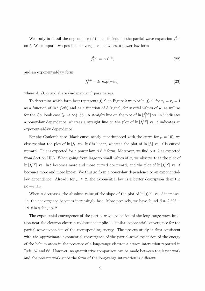
We study in detail the dependence of the coefficients of the partial-wave expansion f lr,µ`
on `. We compare two possible convergence behaviors, a power-law form
f lr,µ` = A `−α, (22)
and an exponential-law form
f lr,µ` = B exp(−β`), (23)
where A, B, α and β are (µ-dependent) parameters.
To determine which form best represents f lr,µ` , in Figure 2 we plot ln |f lr,µ
` | for r1 = r2 = 1
as a function of ln ` (left) and as a function of ` (right), for several values of µ, as well as
for the Coulomb case (µ→∞) [66]. A straight line on the plot of ln |f lr,µ` | vs. ln ` indicates
a power-law dependence, whereas a straight line on the plot of ln |f lr,µ` | vs. ` indicates an
exponential-law dependence.
For the Coulomb case (black curve nearly superimposed with the curve for µ = 10), we
observe that the plot of ln |f`| vs. ln ` is linear, whereas the plot of ln |f`| vs. ` is curved
upward. This is expected for a power law A `−α form. Moreover, we find α ≈ 2 as expected
from Section III A. When going from large to small values of µ, we observe that the plot of
ln |f lr,µ` | vs. ln ` becomes more and more curved downward, and the plot of ln |f lr,µ
` | vs. `
becomes more and more linear. We thus go from a power-law dependence to an exponential-
law dependence. Already for µ ≤ 2, the exponential law is a better description than the
power law.
When µ decreases, the absolute value of the slope of the plot of ln |f lr,µ` | vs. ` increases,
i.e. the convergence becomes increasingly fast. More precisely, we have found β ≈ 2.598 −1.918 lnµ for µ ≤ 2.
The exponential convergence of the partial-wave expansion of the long-range wave func-
tion near the electron-electron coalescence implies a similar exponential convergence for the
partial-wave expansion of the corresponding energy. The present study is thus consistent
with the approximate exponential convergence of the partial-wave expansion of the energy
of the helium atom in the presence of a long-range electron-electron interaction reported in
Refs. 67 and 68. However, no quantitative comparison can be made between the latter work
and the present work since the form of the long-range interaction is different.
9

IV. CONVERGENCE IN ONE-ELECTRON ATOMIC BASIS SETS
In this section, we study the convergence of the long-range wave function and correlation
energy with respect to the size of the one-particle atomic basis. This problem is closely
related to the convergence of the partial-wave expansion studied in the previous section.
Indeed, for a two-electron atom in a singlet S state, it is possible to use the spherical-
harmonic addition theorem to obtain the partial-wave expansion in terms of the relative
angle θ between two electrons by products of the spherical harmonic part Y`,m of the one-
particle atomic basis functions
P`(cos θ) =4π
2`+ 1
∑
m=−`(−1)mY`,m(θ1, φ1)Y`,−m(θ2, φ2), (24)
where cos θ = cos θ1 cos θ2+sin θ1 sin θ2 cos(φ1−φ2) with spherical angles θ1,φ1 and θ2,φ2. The
partial-wave expansion can thus be obtained from a one-particle atomic basis, provided that
the basis saturates the radial degree of freedom for each angular momentum `. In practice,
of course, for the basis sets that we use, this latter condition is not satisfied. Nevertheless,
one can expect the convergence with the maximal angular momentum L of the basis to be
similar to the convergence of the partial-wave expansion.
For this study, we have analyzed the behavior of He, Ne, N2, and H2O at the same
experimental geometries used in Ref. 44 (RN−N = 1.0977 A, RO−H = 0.9572 A and HOH =
104.52). We performed all the calculations with the program MOLPRO 2012 [69] using
Dunning correlation-consistent cc-p(C)VXZ basis sets for which we studied the convergence
with respect to the cardinal number X, corresponding to a maximal angular momentum
of L = X − 1 for He and L = X for atoms from Li to Ne. We emphasize that the series
of Dunning basis sets does not correspond to a partial-wave expansion but to a principal
expansion [70, 71] with maximal quantum number N = X for He and N = X + 1 for
Li to Ne. The short-range exchange-correlation PBE density functional of Ref. 18 (which
corresponds to a slight modification of the one of Ref. 72) was used in all range-separated
calculations.
10

Her1
r2θ
0.20
0.21
0.22
0.23
0.24
0.25
0.26
0.27
0.28
0.29
-180 -120 -60 0 60 120 180
Ψ (
a.
u.)
θ (degree)
HFVDZVTZVQZV5ZV6Z
Hylleraas0.20
0.21
0.22
0.23
0.24
0.25
0.26
0.27
0.28
0.29
-180 -120 -60 0 60 120 180
Ψlr
,µ (
a.
u.)
θ (degree)
RSHVDZVTZVQZV5ZV6Z
0.266
0.267
0.268
0.269
-120 -60 0 60 120
FIG. 3. FCI wave function of the He atom at the Cartesian electron coordinates r1 = (0.5, 0., 0.)
bohr and r2 = (0.5 cos θ, 0.5 sin θ, 0.) bohr, calculated with Dunning basis sets ranging from cc-
pVDZ to cc-pV6Z (abbreviated as VXZ) and shown as a function of the relative angle θ, for the
standard Coulomb interaction case (left) and the long-range interaction case for µ = 0.5 bohr−1
(right). For the case of the Coulomb interaction, an essentially exact curve has been calculated
with a highly accurate 418-term Hylleraas-type wave function [73–75]. For comparison, we also
show the results obtained with the single-determinant HF and RSH wave functions (with the cc-
pV6Z basis) which just give horizontal lines since they do not depend on θ. In the insert plot on
the right, the V5Z and V6Z curves are superimposed.
A. Convergence of the wave function
We start by analyzing the convergence of the FCI ground-state wave function of the He
atom with respect to the cardinal number X of the cc-pVXZ basis sets. We perform a FCI
calculation with the long-range Hamiltonian in Eq. (3) using a fixed RSH density, calcu-
lated from the orbitals obtained in Eq. (4), in the short-range Hartree–exchange-correlation
potential. To facilitate the extraction of the wave function from the program, we use the
Lowdin-Shull diagonal representation of the spatial part of the FCI wave function in terms
of the spatial natural orbitals (NO) ϕµi [76, 77]
Ψlr,µ(r1, r2) =∑
i≥1
cµi ϕµi (r1)ϕµi (r2), (25)
where the coefficients cµi are related to the NO occupation numbers nµi by the relation
nµi = 2|cµi |2. As the signs of cµi are undetermined we have chosen a positive leading coefficient
cµ1 =√nµ1/2, and we assumed that all the other coefficients are negative cµi = −
√nµi /2 for
i ≥ 2 [78]. Even though it has been shown that, for the case of the Coulomb interaction,
11
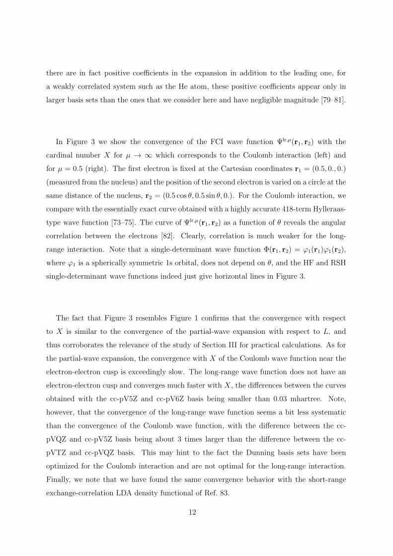
there are in fact positive coefficients in the expansion in addition to the leading one, for
a weakly correlated system such as the He atom, these positive coefficients appear only in
larger basis sets than the ones that we consider here and have negligible magnitude [79–81].
In Figure 3 we show the convergence of the FCI wave function Ψlr,µ(r1, r2) with the
cardinal number X for µ → ∞ which corresponds to the Coulomb interaction (left) and
for µ = 0.5 (right). The first electron is fixed at the Cartesian coordinates r1 = (0.5, 0., 0.)
(measured from the nucleus) and the position of the second electron is varied on a circle at the
same distance of the nucleus, r2 = (0.5 cos θ, 0.5 sin θ, 0.). For the Coulomb interaction, we
compare with the essentially exact curve obtained with a highly accurate 418-term Hylleraas-
type wave function [73–75]. The curve of Ψlr,µ(r1, r2) as a function of θ reveals the angular
correlation between the electrons [82]. Clearly, correlation is much weaker for the long-
range interaction. Note that a single-determinant wave function Φ(r1, r2) = ϕ1(r1)ϕ1(r2),
where ϕ1 is a spherically symmetric 1s orbital, does not depend on θ, and the HF and RSH
single-determinant wave functions indeed just give horizontal lines in Figure 3.
The fact that Figure 3 resembles Figure 1 confirms that the convergence with respect
to X is similar to the convergence of the partial-wave expansion with respect to L, and
thus corroborates the relevance of the study of Section III for practical calculations. As for
the partial-wave expansion, the convergence with X of the Coulomb wave function near the
electron-electron cusp is exceedingly slow. The long-range wave function does not have an
electron-electron cusp and converges much faster with X, the differences between the curves
obtained with the cc-pV5Z and cc-pV6Z basis being smaller than 0.03 mhartree. Note,
however, that the convergence of the long-range wave function seems a bit less systematic
than the convergence of the Coulomb wave function, with the difference between the cc-
pVQZ and cc-pV5Z basis being about 3 times larger than the difference between the cc-
pVTZ and cc-pVQZ basis. This may hint to the fact the Dunning basis sets have been
optimized for the Coulomb interaction and are not optimal for the long-range interaction.
Finally, we note that we have found the same convergence behavior with the short-range
exchange-correlation LDA density functional of Ref. 83.
12

TABLE I. Valence MP2 correlation energies and their errors (in mhartree) for the Coulomb interac-
tion (Ec and ∆Ec) and the long-range interaction at µ = 0.5 bohr−1 (Elr,µc and ∆Elr,µ
c ) calculated
with Dunning basis sets of increasing sizes for He, Ne, N2 and H2O. The errors are calculated with
respect to the estimated CBS limit for the Coulomb interaction and with respect to the cc-pV6Z
values for the long-range interaction.
Coulomb interaction
He Ne N2 H2O
Basis Ec ∆Ec Ec ∆Ec Ec ∆Ec Ec ∆Ec
cc-pVDZ -25.828 11.549 -185.523 134.577 -306.297 114.903 -201.621 98.479
cc-pVTZ -33.138 4.239 -264.323 55.777 -373.683 47.517 -261.462 38.638
cc-pVQZ -35.478 1.899 -293.573 26.527 -398.749 22.451 -282.798 17.302
cc-pV5Z -36.407 0.970 -306.166 13.934 -409.115 12.085 -291.507 8.593
cc-pV6Z -36.807 0.570 -311.790 8.310 -413.823 7.377 -295.205 4.895
CBS limit -37.377a -320(1)b -421(2)b -300(1)b
Long-range interaction
He Ne N2 H2O
Basis Elr,µc ∆Elr,µ
c Elr,µc ∆Elr,µ
c Elr,µc ∆Elr,µ
c Elr,µc ∆Elr,µ
c
cc-pVDZ -0.131 0.227 -0.692 1.963 -20.178 3.316 -6.462 3.532
cc-pVTZ -0.262 0.096 -1.776 0.879 -22.663 0.830 -8.956 1.038
cc-pVQZ -0.322 0.036 -2.327 0.328 -23.263 0.231 -9.626 0.367
cc-pV5Z -0.346 0.012 -2.557 0.098 -23.430 0.064 -9.901 0.092
cc-pV6Z -0.358 -2.655 -23.494 -9.993
aTaken from Ref. 84 where it was obtained by a Gaussian-type geminal MP2 calculation.
bTaken from Ref. 44 where it was estimated from R12-MP2 calculations.
B. Convergence of the correlation energy
We also study the basis convergence of the long-range MP2 correlation energy, given in
Eq. (7), calculated with RSH orbitals for He, Ne, N2 and H2O.
In Table I we show the valence MP2 correlation energies and their errors as a function
13

of the cardinal number X of the cc-pVXZ basis sets for X ≤ 6. We compare the long-
range MP2 correlation energies Elr,µc,X at µ = 0.5 and the standard Coulomb MP2 correlation
energies Ec,X corresponding to µ → ∞. For the case of the Coulomb interaction, the error
is calculated as ∆Ec,X = Ec,X − Ec,∞ where Ec,∞ is the MP2 correlation energy in the
estimated CBS limit taken from Refs. 44 and 84. For the range-separated case we do not
have an independent estimate of the CBS limit of the long-range MP2 correlation energy for
a given value of µ. Observing that the difference between the long-range MP2 correlation
energies for X = 5 and X = 6 is below 0.1 mhartree for µ = 0.5, we choose the cc-pV6Z
result as a good estimate of the CBS limit. Of course, the accuracy of this CBS estimate
will deteriorate for larger values of µ, but in practice this is a good estimate for the range
of values of µ in which we are interested, i.e. 0 ≤ µ ≤ 1 [85]. The error on the long-range
correlation energy is thus calculated as ∆Elr,µc,X = Elr,µ
c,X − Elr,µc,6 .
The first observation to be made is that the long-range MP2 correlation energies only
represent about 1 to 5 % of the Coulomb MP2 correlation energies. Although the long-range
correlation energy may appear small, it is nevertheless essential for the description of dis-
persion interactions for instance. The errors on the long-range MP2 correlation energies are
also about two orders of magnitude smaller than the errors on the Coulomb MP2 correlation
energies.
Inspired by Ref. 60, we compare two possible forms of convergence for the correlation
energy: a power-law form
Elr,µc,X = Elr,µ
c,∞ + AX−α, (26)
and an exponential-law form
Elr,µc,X = Elr,µ
c,∞ +B exp(−βX), (27)
where Elr,µc,∞ is the CBS limit of the long-range correlation energy and A, B, α, and β are
parameters depending on µ, as in Section III. In practice, we actually make linear fits of the
logarithm of the error ln(∆Elr,µc,X) for the two forms:
ln(∆Elr,µc,X) = lnA− α lnX, (28)
ln(∆Elr,µc,X) = lnB − βX. (29)
In Table II, we show the results of the fits for the Coulomb interaction and the long-range
interaction at µ = 0.5 using either the complete range of X or excluding the value for X = 2.
14

TABLE II. Results of the fits to the power and exponential laws of the Coulomb valence MP2
correlation energy error ∆Ec,X and long-range valence MP2 correlation energy error ∆Elr,µc,X for
µ = 0.5 bohr−1. Different ranges, Xmin ≤ X ≤ Xmax, for the cardinal number X of the Dunning
basis sets are tested. The parameters A and B are in mhartree. The squared Pearson correlation
coefficients r2 of the fits are indicated in %. For each line, the largest value of r2 is indicated in
boldface.
Coulomb interaction
Power law Exponential law
Xmin Xmax α A r2 β B r2
He 2 6 2.749 81.84 99.82 0.749 44.04 98.55
3 6 2.902 104.00 99.97 0.669 29.51 99.19
Ne 2 6 2.543 843.36 99.59 0.696 479.76 99.00
3 6 2.754 1169.90 99.93 0.636 355.28 99.37
N2 2 6 2.513 697.74 99.71 0.686 397.67 98.76
3 6 2.693 923.76 99.98 0.621 286.90 99.16
H2O 2 6 2.742 717.04 99.52 0.751 391.27 99.09
3 6 2.988 1051.28 99.92 0.690 288.61 99.39
Long-range interaction
Power law Exponential law
Xmin Xmax α A r2 β B r2
He 2 5 3.128 2.35 96.71 0.974 1.68 99.77
3 5 3.997 8.16 99.11 1.028 2.13 99.95
Ne 2 5 3.189 22.06 95.04 0.998 15.97 99.18
3 5 4.257 101.51 98.27 1.098 24.57 99.65
N2 2 5 4.257 73.26 98.63 1.313 44.49 99.97
3 5 4.997 211.13 99.44 1.283 39.08 99.99
H2O 2 5 3.861 60.27 97.30 1.198 39.24 99.72
3 5 4.686 196.20 97.63 1.210 41.50 99.33
15

We use the squared Pearson correlation coefficient r2 as a measure of the quality of the fit.
For the Coulomb interaction and for all the systems studied, the best fit is achieved with
the power law AX−α with α ≈ 2.5 − 3, which is roughly what is expected [44]. We note
however that the fits to the exponential law are also very good with r2 > 99% when the
X = 2 value is excluded. This explains why extrapolations of the total energy based on an
exponential formula have also been used for the case of the Coulomb interaction [45, 48].
For the case of the long-range interaction, the difference between the fits to the power
law and to the exponential law is much bigger. The best fit is by far obtained for the
exponential law with r2 > 99% for all systems and ranges of X considered. This exponential
convergence of the long-range correlation energy with respect to X is in accordance with
the exponential convergence of the partial-wave expansion of the long-range wave-function
observed in Section III.
We have also performed fits for several other values of µ between 0.1 and 1 and always
obtained an exponential convergence of the long-range valence MP2 correlation energy with
respect to X. However, contrary to what was observed for the partial-wave expansion, we
found that when µ decreases β also decreases a bit for the four systems considered. In other
words, when the interaction becomes more long range, the convergence of the long-range
correlation energy becomes slower. This surprising result may be due to the fact that the
cc-pV6Z result may not be as good an estimate of the CBS limit when µ increases. When
µ decreases, the prefactor B decreases and goes to zero for µ = 0, as expected. Moreover,
we have also checked that we obtain very similar results for the long-range all-electron MP2
correlation energy (including core excitations) with cc-pCVXZ basis sets.
We note that Prendergast et al. [86] have argued that the removal of the electron-electron
cusp in a small region around the coalescence point does not significantly improve the con-
vergence of the energy in the millihartree level of accuracy. At first sight, their conclusion
might appear to be in contradiction with our observation of the exponential convergence
of the long-range correlation energy with X. There are however important differences be-
tween the two studies: (1) their form of long-range interaction is different from ours, (2)
they consider interelectronic distance “cutoffs” of rc . 0.8 bohr whereas we consider larger
“cutoffs” rc = 1/µ ≥ 1 bohr, (3) they do not investigate exponential-law versus power-law
convergence.
Finally, in the Appendix we provide a complement analysis of the basis convergence of the
16

correlation energy of the He atom for truncated configuration-interaction (CI) calculations
in natural orbitals. The analysis shows that, contrary to the case of the Coulomb interaction,
the convergence of the long-range correlation energy is no longer limited by the truncation
rank the CI wave function but by the basis convergence of the natural orbitals themselves.
This result is consistent with an exponential basis convergence of the long-range correlation
energy.
C. Extrapolation scheme
For the long-range interaction case, since both the RSH energy and the long-range cor-
relation energy have an exponential convergence with respect to the cardinal number X, we
propose to extrapolate the total energy to the CBS limit by using a three-point extrapola-
tion scheme based on an exponential formula. Suppose that we have calculated three total
energies EX , EY , EZ for three consecutive cardinal numbers X, Y = X + 1, Z = X + 2. If
we write
EX = E∞ +B exp(−βX), (30)
EY = E∞ +B exp(−βY ), (31)
EZ = E∞ +B exp(−βZ), (32)
and eliminate the unknown parameters B and β, we obtain the following estimate of the
CBS-limit total energy E∞
E∞ = EXY Z =E2Y − EXEZ
2EY − EX − EZ. (33)
In Table III, we report the errors on the RSH+lrMP2 total energy, Eµ = EµRSH +Elr,µ
c,MP2,
obtained with the three-point extrapolation formula using either X = 2, Y = 3, Z = 4
(∆EµDTQ) or X = 3, Y = 4, Z = 5 (∆Eµ
TQ5), and we compare with the errors obtained with
each cc-pVXZ basis set from X = 2 to X = 5 (∆EµX). Here again the errors are calculated
with respect to the cc-pV6Z total energy, for several values of the range-separation parameter
µ = 0.1, 0.5, 1.0, and only valence excitations are included in the MP2 calculations. For all
the systems studied the errors ∆EµDTQ are less than 1.5 mhartree. For Ne, N2, and H2O,
these ∆EµDTQ errors are significantly smaller (by a factor of about 3 to 15) than the errors
∆EµQ obtained with the largest basis used for the extrapolation, and are overall comparable
17

TABLE III. Errors (in mhartree) on the total RSH+lrMP2 energy, Eµ = EµRSH +Elr,µc,MP2, obtained
with cc-pVXZ basis sets from X = 2 to X = 5 (∆EµX = EµX − Eµ6 ) and with the three-point
extrapolation formula of Eq. (33) using X = 2, Y = 3, Z = 4 (∆EµDTQ = EµDTQ − Eµ6 ) or X = 3,
Y = 4, Z = 5 (∆EµTQ5 = EµTQ5−Eµ6 ). The errors are calculated with respect to the cc-pV6Z total
energy for several values of the range-separation parameter µ (in bohr−1). Only valence excitations
are included in the MP2 calculations.
µ ∆EµD ∆EµT ∆EµQ ∆Eµ5 ∆EµDTQ ∆EµTQ5
He 0.1 8.508 0.772 0.261 0.089 0.224 0.003
0.5 8.488 0.781 0.245 0.078 0.205 0.002
1.0 8.258 0.924 0.259 0.078 0.192 0.011
Ne 0.1 72.999 20.215 5.842 0.716 0.464 -2.127
0.5 74.523 20.337 5.763 0.751 0.401 -1.876
1.0 79.311 20.962 5.726 0.803 0.342 -1.548
N2 0.1 47.061 13.026 4.136 0.853 0.993 -1.069
0.5 51.581 13.406 4.090 0.810 1.083 -0.972
1.0 61.053 15.108 4.513 0.868 1.337 -1.043
H2O 0.1 54.861 15.229 5.005 0.857 1.451 -1.975
0.5 55.850 14.736 4.499 0.726 1.105 -1.475
1.0 61.013 15.212 4.423 0.724 1.099 -1.206
with the errors ∆Eµ5 . Thus, the three-point extrapolation formula with X = 2, Y = 3,
Z = 4 provides a useful CBS extrapolation scheme for range-separated DFT. Except for
He, the errors ∆EµTQ5 are negative (i.e. , the extrapolation overshoots the CBS limit) and
larger than the errors ∆Eµ5 . Thus, the three-point extrapolation scheme with X = 3, Y = 4,
Z = 5 does not seem to be useful.
These conclusions extend to calculations including core excitations with cc-pCVXZ basis
sets, which are presented in Table IV. All the errors are smaller than for the valence-only
calculations. The errors ∆EµDTQ are now less than 0.9 mhartree, and are smaller or compa-
rable to the errors ∆Eµ5 . The errors ∆Eµ
TQ5 are always negative and are overall larger than
the errors ∆EµDTQ.
18

TABLE IV. Errors (in mhartree) on the total RSH+lrMP2 energy, Eµ = EµRSH +Elr,µc,MP2, obtained
with cc-pCVXZ basis sets from X = 2 to X = 5 (∆EµX = EµX − Eµ6 ) and with the three-point
extrapolation formula of Eq. (33) using X = 2, Y = 3, Z = 4 (∆EµDTQ = EµDTQ − Eµ6 ) or X = 3,
Y = 4, Z = 5 (∆EµTQ5 = EµTQ5 − Eµ6 ). The errors are calculated with respect to the cc-pCV6Z
total energy for several values of the range-separation parameter µ (in bohr−1). Core excitations
are included in the MP2 calculations.
µ ∆EµD ∆EµT ∆EµQ ∆Eµ5 ∆EµDTQ ∆EµTQ5
Ne 0.1 70.932 18.941 4.929 0.522 -0.240 -1.501
0.5 72.501 18.990 4.831 0.537 -0.263 -1.333
1.0 77.497 19.517 4.775 0.554 -0.250 -1.140
N2 0.1 43.528 10.237 2.334 0.459 -0.126 -0.125
0.5 48.079 10.451 2.285 0.413 0.021 -0.144
1.0 57.942 12.118 2.677 0.467 0.227 -0.209
H2O 0.1 52.875 13.897 4.132 0.680 0.868 -1.208
0.5 53.936 13.350 3.614 0.534 0.541 -0.891
1.0 59.290 13.789 3.527 0.521 0.539 -0.724
We have also tested a more flexible extrapolation scheme where the RSH energy and
the long-range MP2 correlation energy are exponentially extrapolated independently but we
have not found significant differences. On the contrary, one may want to use a less flexible
two-point extrapolation formula using a predetermined value for β. The difficulty with such
an approach is to choose the value of β, which in principle should depend on the system, on
the range-separated parameter µ, and on the long-range wave-function method used. For
this reason, we do not consider two-point extrapolation schemes.
V. CONCLUSIONS
We have studied in detail the basis convergence of range-separated DFT. We have shown
that the partial-wave expansion of the long-range wave function near the electron-electron
coalescence converges exponentially with the maximal angular momentum L. We have also
demonstrated on four systems (He, Ne, N2, and H2O) that the long-range MP2 correla-
19

tion energy converges exponentially with the cardinal number X of the Dunning basis sets
cc-p(C)VXZ. This contrasts with the slow X−3 convergence of the correlation energy for
the standard case of the Coulomb interaction. Due to this exponential convergence, the
extrapolation to the CBS limit is less necessary for range-separated DFT than for standard
correlated wave function methods. Nevertheless, we have proposed a CBS extrapolation
scheme for the total energy in range-separated DFT based on an exponential formula using
calculations from three cardinal numbers X. For the systems studied, the extrapolation
using X = 2, 3, 4 gives an error on the total energy with respect to the estimated CBS limit
which is always smaller than the error obtained with a single calculation at X = 4, and
which is often comparable or smaller than the error obtained with a calculation at X = 5.
We expect the same convergence behavior for range-separated DFT methods in which
the long-range part is treated by configuration interaction, coupled-cluster theory, random-
phase approximations, or density-matrix functional theory. Finally, it should be pointed out
that this rapid convergence is obtained in spite of the fact that the Dunning basis sets have
been optimized for the case of the standard Coulomb interaction. The construction of basis
sets specially optimized for the case of the long-range interaction may give yet a faster and
more systematic convergence.
ACKNOWLEDGEMENTS
We thank Andreas Savin, Trygve Helgaker, Eric Cances, and Gabriel Stoltz for insightful
discussions. This work was supported by French state funds managed by CALSIMLAB and
the ANR within the Investissements d’Avenir program under reference ANR-11-IDEX-0004-
02.
Appendix A: Convergence of the correlation energy for truncated CI calculations
In this Appendix, we explore the basis convergence of the correlation energy of the He
atom for truncated CI calculations for both the Coulomb and long-range interactions. For
a given basis set and interaction, we start by performing a FCI calculation and generating
the corresponding natural orbitals. We then use these natural orbitals in truncated CI
calculations for increasing orbital active spaces 1s2s, 1s2s2p, 1s2s2p3s, 1s2s2p3s3p, and
20

TABLE V. Truncated CI correlation energies (in mhartree) of the He atom for the Coulomb
interaction and for the long-range interaction (at µ = 0.5 bohr−1) for different Dunning basis sets
cc-pVXZ (abbreviated as VXZ) and truncation ranks.
Coulomb interaction
rank VDZ VTZ VQZ V5Z V6Z
1s2s -14.997 -15.806 -16.087 -16.204 -16.212
1s2s2p -32.434 -35.256 -35.664 -35.794 -35.808
1s2s2p3s -35.909 -36.425 -36.595 -36.618
1s2s2p3s3p -37.448 -38.068 -38.261 -38.291
1s2s2p3s3p3d -39.079 -39.807 -39.999 -40.028
Long-range interaction
rank VDZ VTZ VQZ V5Z V6Z
1s2s -0.018 -0.036 -0.038 -0.039 -0.039
1s2s2p -0.155 -0.329 -0.415 -0.449 -0.468
1s2s2p3s -0.329 -0.415 -0.450 -0.468
1s2s2p3s3p -0.329 -0.415 -0.450 -0.469
1s2s2p3s3p3d -0.329 -0.416 -0.451 -0.470
1s2s2p3s3p3d. Table V shows the Coulomb and long-range correlation energies for the
different basis sets and truncation ranks. For the Coulomb interaction, the correlation
energy for a fixed rank converges rapidly with the basis size, while the convergence with
respect to the rank is much slower. For the long-range interaction, the correlation energy
jumps by one order of magnitude when including the 2p natural orbital, which is consistent
with the fact that the long-range interaction brings in first angular correlation effects [87].
The long-range correlation energy is essentially converged at rank 1s2s2p, and the overall
convergence is now determined by the basis convergence of the natural orbitals.
Finally, we compare two possible forms for the convergence of the truncated CI corre-
lation energies with the cardinal number X, the power law Eq. (26) and the exponential
law Eq. (27). Using as reference the results obtained with the cc-pV6Z basis set, we have
calculated for the different truncation ranks the correlation energy errors for the Coulomb
21

TABLE VI. Results of the fits to the power and exponential laws of the truncated CI correlation
energy error for the Coulomb interaction, ∆Ec,X = Ec,X − Ec,6, and the long-range interaction,
∆Elr,µc,X = Elr,µ
c,X − Elr,µc,6 for µ = 0.5 bohr−1. The range for the cardinal number X of the Dunning
basis sets is 2 ≤ X ≤ 6 for the 1s2s and 1s2s2p ranks, and 3 ≤ X ≤ 6 for all the larger ranks. The
parameters A and B are in mhartree. The squared Pearson correlation coefficients r2 of the fits
are indicated in %. For each line, the largest value of r2 is indicated in boldface.
Coulomb interaction
Power law Exponential law
rank α A r2 β B r2
1s2s 5.081 65.641 87.44 1.618 43.148 94.39
1s2s2p 5.765 241.923 95.45 1.797 131.516 98.80
1s2s2p3s 6.616 1219.794 95.63 1.716 140.022 98.11
1s2s2p3s3p 6.440 1168.927 96.46 1.668 140.605 98.65
1s2s2p3s3p3d 6.771 1874.080 97.16 1.751 200.085 99.07
Long-range interaction
Power law Exponential law
rank α A r2 β B r2
1s2s 3.974 0.321 99.45 1.206 0.188 97.51
1s2s2p 3.058 3.108 96.28 0.953 2.249 99.64
1s2s2p3s 3.956 11.283 99.01 1.018 2.991 99.93
1s2s2p3s3p 3.927 10.979 99.02 1.010 2.938 99.93
1s2s2p3s3p3d 3.892 10.701 99.00 1.001 2.898 99.93
interaction, ∆Ec,X = Ec,X − Ec,6, and for the long-range interaction, ∆Elr,µc,X = Elr,µ
c,X − Elr,µc,6 ,
and performed logarithmic fits as in Section IV B. Table VI shows the results of the fits. For
both the Coulomb and long-range interactions, for the rank 1s2s2p and larger, the best fit
is achieved with the exponential law B exp(−βX). Thus, in comparison with the Coulomb
interaction, the long-range interaction does not significantly change the basis convergence of
22

the correlation energy at a fixed truncation rank. However, for the long-range interaction,
this exponential convergence at a fixed truncation rank becomes the dominant limitation to
the overall basis convergence.
[1] J. Toulouse, F. Colonna, and A. Savin, Phys. Rev. A 70, 062505 (2004).
[2] P. Hohenberg and W. Kohn, Phys. Rev. 136, B 864 (1964).
[3] W. Kohn and L. J. Sham, Phys. Rev. 140, A1133 (1965).
[4] J. G. Angyan, I. C. Gerber, A. Savin, and J. Toulouse, Phys. Rev. A 72, 012510 (2005).
[5] I. C. Gerber and J. G. Angyan, Chem. Phys. Lett. 416, 370 (2005).
[6] I. C. Gerber and J. G. Angyan, J. Chem. Phys. 126, 044103 (2007).
[7] J. G. Angyan, Phys. Rev. A 78, 022510 (2008).
[8] E. Fromager and H. J. A. Jensen, Phys. Rev. A 78, 022504 (2008).
[9] E. Goll, T. Leininger, F. R. Manby, A. Mitrushchenkov, H.-J. Werner, and H. Stoll, Phys.
Chem. Chem. Phys. 10, 3353 (2008).
[10] B. G. Janesko and G. E. Scuseria, Phys. Chem. Chem. Phys. 11, 9677 (2009).
[11] E. Fromager, R. Cimiraglia, and H. J. A. Jensen, Phys. Rev. A 81, 024502 (2010).
[12] S. Chabbal, H. Stoll, H.-J. Werner, and T. Leininger, Mol. Phys. 108, 3373 (2010).
[13] S. Chabbal, D. Jacquemin, C. Adamo, H. Stoll, and T. Leininger, J. Chem. Phys. 133, 151104
(2010).
[14] E. Fromager and H. J. A. Jensen, J. Chem. Phys. 135, 034116 (2011).
[15] O. Kullie and T. Saue, Chem. Phys. 395, 54 (2011).
[16] Y. Cornaton, A. Stoyanova, H. J. A. Jensen, and E. Fromager, Phys. Rev. A 88, 022516
(2013).
[17] E. Goll, H.-J. Werner, and H. Stoll, Phys. Chem. Chem. Phys. 7, 3917 (2005).
[18] E. Goll, H.-J. Werner, H. Stoll, T. Leininger, P. Gori-Giorgi, and A. Savin, Chem. Phys. 329,
276 (2006).
[19] E. Goll, H. Stoll, C. Thierfelder, and P. Schwerdtfeger, Phys. Rev. A 76, 032507 (2007).
[20] E. Goll, H.-J. Werner, and H. Stoll, Chem. Phys. 346, 257 (2008).
[21] E. Goll, M. Ernst, F. Moegle-Hofacker, and H. Stoll, J. Chem. Phys. 130, 234112 (2009).
[22] J. Toulouse, I. C. Gerber, G. Jansen, A. Savin, and J. G. Angyan, Phys. Rev. Lett. 102,
23

096404 (2009).
[23] B. G. Janesko, T. M. Henderson, and G. E. Scuseria, J. Chem. Phys. 130, 081105 (2009).
[24] B. G. Janesko, T. M. Henderson, and G. E. Scuseria, J. Chem. Phys. 131, 034110 (2009).
[25] B. G. Janesko and G. E. Scuseria, J. Chem. Phys. 131, 154106 (2009).
[26] W. Zhu, J. Toulouse, A. Savin, and J. G. Angyan, J. Chem. Phys. 132, 244108 (2010).
[27] J. Toulouse, W. Zhu, J. G. Angyan, and A. Savin, Phys. Rev. A 82, 032502 (2010).
[28] J. Paier, B. G. Janesko, T. M. Henderson, G. E. Scuseria, A. Gruneis, and G. Kresse, J.
Chem. Phys. 132, 094103 (2010).
[29] J. Toulouse, W. Zhu, A. Savin, G. Jansen, and J. G. Angyan, J. Chem. Phys. 135, 084119
(2011).
[30] J. G. Angyan, R.-F. Liu, J. Toulouse, and G. Jansen, J. Chem. Theory Comput. 7, 3116
(2011).
[31] R. M. Irelan, T. M. Henderson, and G. E. Scuseria, J. Chem. Phys. 135, 094105 (2011).
[32] T. Gould and J. F. Dobson, Phys. Rev. B 84, 241108 (2011).
[33] E. Chermak, B. Mussard, J. G. Angyan, and P. Reinhardt, Chem. Phys. Lett. 550, 162
(2012).
[34] B. Mussard, P. G. Szalay, and J. G. Angyan, J. Chem. Theory Comput. 10, 1968 (2014).
[35] T. H. Dunning, J. Chem. Phys. 90, 1007 (1989).
[36] C. Schwartz, Phys. Rev. 126, 1015 (1962).
[37] C. Schwartz, in Methods in Computational Physics, Vol. 2, edited by B. Alder, S. Fernbach,
and M. Rotenberg, pages 241–266, Academic Press, New York and London, 1963.
[38] D. P. Carroll, H. J. Silverstone, and R. M. Metzger, J. Chem. Phys. 71, 4142 (1979).
[39] R. N. Hill, J. Chem. Phys. 83, 1173 (1985).
[40] B. D. Goddard, Siam J. Math. Anal. 41, 77 (2009).
[41] W. Kutzelnigg and J. D. Morgan III, J. Chem. Phys. 96, 4484 (1992).
[42] G. F. Gribakin and J. Ludlow, J. Phys. B 35, 339 (2002).
[43] T. Helgaker, W. Klopper, H. Koch, and J. Noga, J. Chem. Phys. 106, 9639 (1997).
[44] A. Halkier, T. Helgaker, P. Jørgensen, W. Klopper, H. Koch, J. Olsen, and A. K. Wilson,
Chem. Phys. Lett. 286, 243 (1998).
[45] D. Feller, J. Chem. Phys. 96, 6104 (1992).
[46] D. Feller, J. Chem. Phys. 98, 7059 (1993).
24

[47] K. A. Peterson, R. A. Kendall and T. H. Dunning Jr., J. Chem. Phys. 99, 9790 (1993).
[48] K. A. Peterson and T. H. Dunning Jr., J. Phys. Chem. 99, 3898 (1995).
[49] J. M. L. Martin, Chem. Phys. Lett. 259, 669 (1996).
[50] D. G. Truhlar, Chem. Phys. Lett. 294, 45 (1998).
[51] D. Feller, J. Chem. Phys. 138, 074103 (2013).
[52] I. Gerber and J. G. Angyan, Chem. Phys. Lett. 415, 100 (2005).
[53] E. Fromager, J. Toulouse, and H. J. A. Jensen, J. Chem. Phys. 126, 074111 (2007).
[54] T. Leininger, H. Stoll, H.-J. Werner, and A. Savin, Chem. Phys. Lett. 275, 151 (1997).
[55] R. Pollet, A. Savin, T. Leininger, and H. Stoll, J. Chem. Phys. 116, 1250 (2002).
[56] J. K. Pedersen and H. J. A. Jensen, A second order MCSCF-DFT hybrid algorithm (unpub-
lished).
[57] E. Fromager, F. Real, P. Wahlin, U. Wahlgren, and H. J. A. Jensen, J. Chem. Phys. 131,
054107 (2009).
[58] K. Pernal, Phys. Rev. A 81, 052511 (2010).
[59] D. R. Rohr, J. Toulouse, and K. Pernal, Phys. Rev. A 82, 052502 (2010).
[60] A. Halkier, T. Helgaker, P. Jørgensen, W. Klopper, and J. Olsen, Chem. Phys. Lett. 302,
437 (1999).
[61] T. Kato, Comm. Pure Appl. Math. 10, 151 (1957).
[62] W. Kutzelnigg, Theor. Chem. Acta 68, 445 (1985).
[63] Note that the partial-wave expansion of any odd power of r12 contains an infinite number of
terms. In contrast, the partial-wave expansion of any even power of r12 terminates at a finite
`.
[64] P. Gori-Giorgi and A. Savin, Phys. Rev. A 73, 032506 (2006).
[65] Wolfram Research, Inc., Mathematica, Version 9.0, Champaign, IL (2012).
[66] For r1 = r2, f lr,µ` > 0 for ` = 0 and f lr,µ
` < 0 for ` ≥ 1.
[67] I. Sirbu and H. F. King, J. Chem. Phys. 117, 6411 (2002).
[68] I. Sirbu and H. F. King, Int. J. Quantum Chem. 92, 433 (2003).
[69] H.-J. Werner, P. J. Knowles, G. Knizia, F. R. Manby, M. Schutz, and others, Molpro, version
2012.1, a package of ab initio programs, Cardiff, UK, 2012, see http://www.molpro.net.
[70] W. Klopper, K. L. Bak, P. Jørgensen, J. Olsen, and T. Helgaker, J. Phys. B 32, R103 (1999).
[71] T. Helgaker, P. Jørgensen, and J. Olsen, Molecular Electronic-Structure Theory, Wiley,
25

Chichester, 2002.
[72] J. Toulouse, F. Colonna, and A. Savin, J. Chem. Phys. 122, 014110 (2005).
[73] D. E. Freund, B. D. Huxtable, and J. D. Morgan III, Phys. Rev. A 29, 980 (1984).
[74] J. D. Baker, D. E. Freund, R. N. Hill, and J. D. Morgan III, Phys. Rev. A 41, 1247 (1990).
[75] C. J. Umrigar and X. Gonze, Phys. Rev. A 50, 3827 (1994).
[76] P.-O. Lowdin and H. Shull, Phys. Rev. 101, 1730 (1956).
[77] A. Szabo and N. S. Ostlund, Modern Quantum Chemistry: Introduction to Advanced Elec-
tronic Structure Theory, Dover, New York, 1996.
[78] S. Goedecker and C. J. Umrigar, in Many-Electron Densities and Reduced Density Matrices,
edited by J. Cioslowski, pages 165–181, Kluwer Academic, Dordrecht/New York, 2000.
[79] X. W. Sheng, L. M. Mentel, O. V. Gritsenko, and E. J. Baerends, J. Chem. Phys. 138, 164105
(2013).
[80] K. J. H. Giesbertz and R. van Leeuwen, J. Chem. Phys. 139, 104109 (2013).
[81] K. J. H. Giesbertz and R. van Leeuwen, J. Chem. Phys. 139, 104110 (2013).
[82] For a discussion of angular and radial correlation and the shape of the correlation hole in the
He atom with the long-range interaction, see Ref. 87.
[83] S. Paziani, S. Moroni, P. Gori-Giorgi, and G. B. Bachelet, Phys. Rev. B 73, 155111 (2006).
[84] K. Patkowski, W. Cencek, M. Jeziorska, B. Jeziorski, and K. Szalewicz, J. Phys. Chem. A
111, 7611 (2007).
[85] For µ = 1 the difference between the long-range MP2 correlation energies for X = 5 and
X = 6 is still as small as about 0.2 mhartree.
[86] D. Prendergast, M. Nolan, C. Filippi, S. Fahy, and J. C. Greer, J. Chem. Phys. 115, 1626
(2001).
[87] R. Pollet, F. Colonna, T. Leininger, H. Stoll, H.-J. Werner, and A. Savin, Int. J. Quantum.
Chem. 91, 84 (2003).
26

48 BIBLIOGRAPHY

Chapter 3
Self-consistent double-hybrid
density-functional theory using the
optimized-effective-potential method
In this chapter we wanted to compare two approaches to double-hybrid approximations, com-
bining a fraction of Hartree-Fock exchange and MP2 correlation with exchange and correlation
from density-functional approximations. The results of this study has been accepted in The
Journal of Chemical Physics and the manuscript is included in this chapter. The global context
of this work is the definition of a self-consistent range-separated double-hybrid approximation.
The aim of this first study was to compare two approaches for the one-parameter double-hybrid
(1DH) approximation [1]: (i) the standard approach with the MP2 contribution added a poste-
riori and (ii) a self-consistent approach based on the optimized-effective-potential method and
implemented by the team of Prof. Irek Grabowski from the Nicolaus Copernicus University
(Poland).
In this work we chose to compare some chemical properties and especially ionization poten-
tials (IP) and electronic affinities (EA). To calculate those properties with standard 1DH the
derivatives of the energy are calculated by finite differences [2]
−IP =
(∂E1DH
∂N
)
N−δ≈ E1DH(N)− E1DH(N −∆)
∆,
−EA =
(∂E1DH
∂N
)
N+δ
≈ E1DH(N + ∆)− E1DH(N)
∆.
The numerical implementation of IP and EA was done by Bastien Mussard in the Molpro
code [3]. The first part of this work was to perform calculations for 1DH and RSH-MP2 for
different chemical properties. We then compare the results with the results for the self-consistent
1DH (OEP-1DH) made by our collaborators. To compare these data a work on derivative
49

50 BIBLIOGRAPHY
discontinuity was needed for the OEP-1DH method. The comparison of the RSH-MP2 with
self-consistent RSH-MP2 will be part of a later work.
For the standard approach Brillouin’s theorem applies and the single excitations do not con-
tribute to second order. However with self-consistency Brillouin’s theorem does no longer apply
and the single excitations do contribute in the perturbation theory similarly to Gorling-Levy per-
turbation theory [4]. In this study the results of OEP-1DH compared to the standard case only
include double excitations. This choice was made to show modifications due to self-consistency
without the interfering of further modifications. An interesting open question would be to study
the contributions of the single excitations in the OEP-1DH scheme.
Bibliography
[1] K. Sharkas, J. Toulouse and A. Savin. Double-hybrid density-functional theory made rigor-
ous. J. Chem. Phys., 134, 064113, 2011.
[2] A. J. Cohen, P. Mori-Sanchez and W. Yang. Second-Order Perturbation Theory with Frac-
tional Charges and Fractional Spins. J. Chem. Theory. Comput. 5, 786, 2009
[3] B. Mussard and J. Toulouse. Fractional-charge and fractional-spin errors in range-separated
density-functional theory. accepted in Mol. Phys., doi:10.1080/00268976.2016.1213910,
[4] A. Gorling and M. Levy, Phys. Rev. A 50 , 196 1994 ! ; Int. J. Quantum Chem., Quantum
Chem. Symp. 29 ,93 1995.

Self-consistent double-hybrid density-functional theory using the
optimized-effective-potential method
Szymon Smiga1,2,3,∗ Odile Franck4,5,† Bastien Mussard4,5,‡ Adam
Buksztel1,§ Ireneusz Grabowski1,¶ Eleonora Luppi4,∗∗ and Julien Toulouse4††
1Institute of Physics, Faculty of Physics, Astronomy and Informatics,
Nicolaus Copernicus University, 87-100 Torun, Poland
2Istituto Nanoscienze-CNR, Via per Arnesano 16, I-73100 Lecce, Italy
3Center for Biomolecular Nanotechnologies @UNILE,
Istituto Italiano di Tecnologia (IIT),
Via Barsanti, 73010 Arnesano (LE), Italy
4Laboratoire de Chimie Theorique, Universite Pierre et Marie Curie,
CNRS, Sorbonne Universites, F-75005 Paris, France
5Institut des sciences du calcul et des donnees,
Universite Pierre et Marie Curie, Sorbonne Universites, F-75005, Paris, France
(Dated: September 20, 2016)
Abstract
We introduce an orbital-optimized double-hybrid (DH) scheme using the optimized-effective-
potential (OEP) method. The orbitals are optimized using a local potential corresponding to
the complete exchange-correlation energy expression including the second-order Møller-Plesset
(MP2) correlation contribution. We have implemented a one-parameter version of this OEP-
based self-consistent DH scheme using the BLYP density-functional approximation and compared
it to the corresponding non-self-consistent DH scheme for calculations on a few closed-shell atoms
and molecules. While the OEP-based self-consistency does not provide any improvement for the
calculations of ground-state total energies and ionization potentials, it does improve the accuracy
of electron affinities and restores the meaning of the LUMO orbital energy as being connected to a
neutral excitation energy. Moreover, the OEP-based self-consistent DH scheme provides reasonably
accurate exchange-correlation potentials and correlated densities.
∗ [email protected]† [email protected]‡ [email protected]
1

I. INTRODUCTION
Density-functional theory (DFT) [1, 2] is a powerful approach for electronic-structure
calculations of atoms, molecules, and solids. In the Kohn-Sham (KS) formulation, se-
ries of approximations for the exchange-correlation energy have been developed for an
ever-increasing accuracy: local-density approximation (LDA), semilocal approximations
(generalized-gradient approximations (GGA) and meta-GGA), hybrid approximations intro-
ducing a fraction of Hartree-Fock (HF) exchange, and nonlocal correlation approximations
using virtual KS orbitals (see, e.g., Ref. 3 for a recent review).
In the latter family of approximations, the double-hybrid (DH) approximations are be-
coming increasingly popular. Introduced in their current form by Grimme [4], they consist
in combining a semilocal exchange density functional with HF exchange and a semilocal
correlation density functional with second-order Møller-Plesset (MP2) perturbative correla-
tion. Numerous such DH approximations have been developed in the last decade (see Ref. 5
for a review). In general, DH approximations give thermochemistry properties with near-
chemical accuracy for molecular systems without important static correlation effects. In
virtually all applications of DH approximations, the orbitals are calculated within the gen-
eralized KS (GKS) framework [6] (i.e., with a nonlocal HF exchange potential) and without
the presence of the MP2 correlation term. The MP2 contribution is then evaluated using
the previously self-consistently calculated orbitals and added a posteriori to the total energy.
Recently, Peverati and Head-Gordon [7] proposed an orbital-optimized DH scheme where the
orbitals are self-consistently optimized in the presence of the MP2 correlation term. This is
a direct extension of orbital-optimized MP2 schemes in which the MP2 total energy is min-
imized with respect to occupied-virtual orbital rotation parameters [8, 9]. Like for regular
orbital-optimized MP2 method, also here the optimization of orbitals leads to substantial
improvements in spin-unrestricted calculations for symmetry breaking and open-shell sit-
uations. Very recently, an approximate orbital-optimized DH scheme was also proposed
which confirmed the utility of optimizing the orbitals in complicated electronic-structure
problems [10].
In this work, we propose an alternative orbital-optimized DH scheme using the optimized-
§ [email protected]¶ [email protected]∗∗ [email protected]†† [email protected]
2

effective-potential (OEP) method [11, 12] (see Refs. 13–15 for reviews on OEP). The idea
is to optimize the orbitals in the DH total energy expression by using a fully local potential
corresponding to the complete exchange-correlation energy expression including the MP2
contribution. This can be considered as an extension of OEP schemes using a second-order
correlation energy expression [16–20].
In comparison to the previously-mentioned orbital-optimized DH schemes, we expect
that the proposed OEP self-consistent DH scheme to provide additional advantages. First,
there is the appeal of staying within the philosophy of the KS scheme with a local potential.
Second, having a local potential and the associated orbital energies can be useful for interpre-
tative purposes. Third, the OEP approach can be advantageous in calculations of excitation
energies and response properties, similarly to the advantages of using OEP exact exchange
(EXX) versus regular HF. Indeed, contrary to the HF case, with EXX the unoccupied or-
bitals feel a local potential asymptotically decaying as −1/r, allowing it to support many
unoccupied bound states, which are good starting points for calculating high-lying/Rydberg
excitation energies and response properties (see, e.g., Refs. 13, 15, and 21).
The paper is organized as follows. In Section II, we review the theory of the standard
DH approximations and formulate the proposed self-consistent OEP DH approach. We
also explain how the ionization potential and the electron affinity are obtained in both
methods. After providing computational details in Section III, we discuss our results in
Section IV on total energies, ionization potentials, electron affinities, exchange-correlation
and correlation potentials, and correlated densities obtained for a set of atoms (He, Be, Ne,
Ar) and molecules (CO and H2O). Finally, Section V contains our conclusions.
Throughout the paper, we use the convention that i and j indices label occupied spin
orbitals, a and b label virtual ones, and p and q are used for both occupied and virtual spin
orbitals. In all equations Hartree atomic units are assumed.
II. THEORY
A. Standard double-hybrid approximations
For simplicity, in this work, we consider the one-parameter double-hybrid (1DH) approxi-
mation of Ref. 22 in which the density scaling in the correlation functional is neglected. The
3

extension to more general density-scaled or two-parameter double-hybrid approximations [4]
is straightforward. The expression of the total energy is thus written as
E =∑
i
∫ϕ∗i (x)
(−1
2∇2 + vne(r)
)ϕi(x) dx
+EH + E1DHxc , (1)
where ϕi(x) are the occupied spin orbitals with x = (r, σ) indicating space-spin coordinates.
In Eq. (1), vne(r) is the nuclei-electron potential, EH = (1/2)∫∫
n(x1)n(x2)/|r2− r1|dx1dx2
is the Hartree energy written with the spin densities n(x) =∑
i |ϕi(x)|2, and E1DHxc is the
exchange-correlation energy taken as
E1DHxc = E1H
xc + λ2 EMP2c . (2)
In this expression, E1Hxc is the one-parameter hybrid (1H) part of the exchange-correlation
energy
E1Hxc = λEHF
x + (1− λ)EDFAx + (1− λ2)EDFA
c , (3)
and λ (0 6 λ 6 1) is an empirical scaling parameter. The expression of the HF (or exact)
exchange energy is
EHFx = −1
2
∑
i,j
〈ij|ji〉, (4)
where 〈pq|rs〉 =∫∫
dx1dx2ϕ∗p(x1)ϕ
∗q(x2)ϕr(x1)ϕs(x2)/|r2−r1| are the two-electron integrals.
The expression for the MP2 correlation energy is
EMP2c = −1
4
∑
i,j
∑
a,b
|〈ij||ab〉|2εa + εb − εi − εj
, (5)
where 〈ij||ab〉 = 〈ij|ab〉 − 〈ij|ba〉 are the antisymmetrized two-electron integrals, and εp is
the energy of the spin orbital p. Finally, EDFAx and EDFA
c are the semilocal density-functional
approximations (DFA) evaluated at the spin densities n(x). For example, choosing the Becke
88 (B) exchange functional [23] and the Lee-Yang-Parr (LYP) correlation functional [24]
leads to the 1DH-BLYP double-hybrid approximation [22] which is a one-parameter version
of the B2-PLYP approximation [4].
We must stress here that the expression of the correlation energy in Eq. (5) has a standard
MP2 form. However, except for λ = 1, the orbitals are not the HF ones, so the value of
the correlation energy in Eq. (5) calculated with these orbitals does not correspond to
4

the standard MP2 correlation energy. In the DFT context, the most usual second-order
correlation energy expression is given by second-order Gorling-Levy (GL2) perturbation
theory [16, 17], which in addition to the MP2-like double-excitation term also includes a
single-excitation term. In this work, following the standard practice for the double-hybrid
approximations, we do not include the single-excitation term, which is usually two orders of
magnitude smaller than the double-excitation term [25–27].
In the standard DH approximations, the spin orbitals are calculated by disregarding
the MP2 term in Eq. (2) and considering the HF exchange energy as a functional of the
one-particle density matrix n1(x′,x) =
∑i ϕ∗i (x)ϕi(x
′), leading to a GKS equation
(−1
2∇2 + vne(r) + vH(r)
)ϕp(x)
+
∫v1Hxc (x,x′)ϕp(x
′)dx′ = ε1Hp ϕp(x), (6)
where vH(r) =∫n(x′)/|r′ − r|dx′ is the Hartree potential and v1Hxc (x,x′) is the functional
derivative of the three terms in Eq. (3) with respect to n1(x′,x)
v1Hxc (x,x′) =δE1H
xc
δn1(x′,x)
= λvHFx (x,x′) + (1− λ)vDFA
x (x)δ(x− x′)
+(1− λ2)vDFAc (x)δ(x− x′). (7)
In this expression, vHFx (x,x′) = −n1(x,x
′)/|r − r′| is the nonlocal HF potential, while
vDFAx (x) = δEDFA
x /δn(x) and vDFAc (x) = δEDFA
c /δn(x) are the local exchange and corre-
lation DFA potentials, respectively. These 1H orbitals and corresponding orbital energies
ε1Hp are thus used in the MP2 correlation expression of Eq. (5). We recall that for λ = 0
the 1DH method reduces to the standard KS scheme, while for λ = 1 it recovers the stan-
dard MP2 method with HF orbitals. In practice, optimal values of λ are around 0.6-0.8,
depending on the density-functional approximations used [22, 28, 29].
B. Self-consistent OEP double-hybrid approximations
Here, we propose to fully self-consistently calculate the spin orbitals in the DH approxi-
mations by taking into account the MP2 term, and considering the HF exchange energy and
MP2 correlation energy as implicit functionals of the density. Thus, Eq. (6) is replaced by
5

a KS equation(−1
2∇2 + vne(r) + vH(r) + vOEP-1DH
xc (x)
)ϕp(x)
= εpϕp(x), (8)
where vOEP-1DHxc is a fully local potential obtained by taking the functional derivative with
respect to the density of all terms in Eq. (2)
vOEP-1DHxc (x) =
δE1DHxc
δn(x)
= λvEXXx (x) + (1− λ)vDFA
x (x)
+(1− λ2)vDFAc (x) + λ2vGL2
c (x), (9)
where vEXXx (x) = δEHF
x /δn(x) is the EXX potential and vGL2c (x) = δEMP2
c /δn(x) is here
referred to as the GL2 correlation potential (even though it does not contain the single-
excitation term). Since EHFx and EMP2
c are only implicit functionals of the density through
the orbitals and orbital energies, the calculation of vEXXx (x) and vGL2
c (x) must be done with
the OEP method, as done in Refs. 18–20. We note that several alternative methods to
OEP have been proposed [30–36], but we do not consider these alternative methods in this
work. We will refer to the present approach as the OEP-1DH method. As in the case of
the standard DH approach, for λ = 0 the OEP-1DH method reduces to the standard KS
scheme. For λ = 1 it reduces to a correlated OEP scheme with the full MP2-like correlation
energy expression (but without the single-excitation term), here referred to as the OEP-GL2
scheme.
The OEP equations for the EXX exchange and GL2 correlation potentials
∫vEXXx (x′) χs(x
′,x) dx′ = Λx(x), (10)
and ∫vGL2c (x′) χs(x
′,x) dx′ = ΛMP2c (x), (11)
can be obtained after applying a functional-derivative chain rule (see, e.g., Refs. 14, 18, 20,
27, and 37). In these expressions, χs(x′,x) = δn(x′)/δvs(x) is the KS static linear-response
function which can be expressed in terms of spin orbitals and spin orbital energies,
χs(x′,x) = −
∑
i
∑
a
ϕ∗i (x′)ϕa(x′)ϕ∗a(x)ϕi(x)
εa − εi+ c.c., (12)
6

where c.c. stands for the complex conjugate, and vs(x) = vne(r) + vH(r) + vOEP-1DHxc (x) is
the total KS potential. The expressions for Λx(x) and ΛMP2c (x) are, respectively,
Λx(x) =δEHF
x
δvs(x)=∑
i
∫dx′(δEHF
x
δϕi(x′)
δϕi(x′)
δvs(x)+ c.c.
)
=∑
i,j
∑
a
(〈ij|ja〉ϕ
∗a(x)ϕi(x)
εa − εi+ c.c.
), (13)
and
ΛMP2c (x) =
δEMP2c
δvs(x)=∑
p
[∫dx′(δEMP2
c
δϕp(x′)
δϕp(x′)
δvs(x)+ c.c.
)+∂EMP2
c
∂εp
δεpδvs(x)
]
=1
2
∑
i,j
∑
a,b
∑
q 6=i
( 〈ij||ab〉〈ab||qj〉εa + εb − εi − εj
ϕ∗q(x)ϕi(x)
εq − εi+ c.c.
)
+1
2
∑
i,j
∑
a,b
∑
q 6=a
( 〈ij||qb〉〈ab||ij〉εa + εb − εi − εj
ϕ∗q(x)ϕa(x)
εq − εa+ c.c.
)
+1
2
∑
i,j
∑
a,b
|〈ij||ab〉|2(εa + εb − εi − εj)2
(|ϕa(x)|2 − |ϕi(x)|2
). (14)
In practice, in order to solve the OEP equations [Eqs. (10) and (11)], the EXX and GL2
potentials are calculated using expansions in a finite Gaussian basis set [38–42]. The EXX
potential is thus expanded over orthonormalized auxiliary Gaussian basis functions gn(r)as
vEXXx (rσ) = vSlater(rσ) +
∑
n
cσx,n gn(r), (15)
where the Slater potential, vSlater(rσ) = −(1/n(x))∫
dx′|n1(x,x′)|2/|r − r′|, is added to
ensure the correct −1/|r| asymptotic behavior of the potential. Similarly, the GL2 potential
is expanded as
vGL2c (rσ) =
∑
n
cσc,n gn(r). (16)
Expanding as well the linear-response function in the same basis
χs(rσ, r′σ) =
∑
n,m
(Xσ)nmgn(r)gm(r′), (17)
and after using Eq. (10), the coefficients in Eq. (15) are found as
cσx,n =∑
m
(Λx,σ)m(X−1σ )mn − vσSlater,n, (18)
7

where (Λx,σ)m =∫
dr gm(r)Λx(rσ), vσSlater,n =∫
dr gn(r)vSlater(rσ), and (X−1σ )mn are the
elements of the (pseudo-)inverse of the matrix Xσ. Similarly, after using Eq. (11), the
coefficients in Eq. (16) are found as
cσc,n =∑
m
(ΛMP2c,σ )m(X−1σ )mn, (19)
where (ΛMP2c,σ )m =
∫dr gm(r)ΛMP2
c (rσ). In this work, the same basis set is used for expanding
the orbitals and the potentials. In practice, our OEP-1DH calculations employ a truncated
singular-value decomposition (TSVD) method for the construction of the pseudo-inverse of
the linear-response function [used in Eqs. (18) and (19)] to ensure that stable and physically
sound solutions are obtained in the OEP equations [Eqs. (10) and (11)].
In principle, this procedure selects the EXX and GL2 potentials which vanish at |r| → ∞.
We note that, when continuum states are included, the GL2 potential actually diverges at
infinity for finite systems [43–47]. Nevertheless, this problem is avoided when using a discrete
basis set with functions vanishing at infinity (such as the basis set used in this work) [46–
48]. In practice, the calculated potentials can still be shifted by a function which vanishes
at infinity but which is an arbitrary constant in the physically relevant region of space. To
remove this arbitrary constant, as in Ref. 18, we impose the HOMO condition on the EXX
potential
vEXXx,HH = vHF
x,HH , (20)
where vEXXx,HH =
∫ϕ∗H(x)vEXX
x (x)ϕH(x)dx and vHFx,HH =
∫∫ϕ∗H(x)vHF
x (x,x′)ϕH(x′)dxdx′ =
−∑j〈Hj|jH〉 are the expectation values of the EXX and HF exchange potentials over the
HOMO spin orbital referred to as H. Similarly, we impose the HOMO condition on the GL2
potential
vGL2c,HH = ΣMP2
c,HH(εH), (21)
where vGL2c,HH =
∫ϕ∗H(x)vGL2
c (x)ϕH(x)dx and ΣMP2c,HH(εH) =
∫∫ϕ∗H(x)ΣMP2
c (x,x′; εH)ϕH(x′)dxdx′
are the expectation values of the GL2 local potential and of the MP2 self-energy over
the HOMO spin orbital. The MP2 self-energy is defined as the functional derivative of
EMP2c with respect to the one-particle Green function G(x′,x;ω), i.e. ΣMP2
c (x,x′;ω) =
8

2πi δEMP2c /δG(x′,x;ω), and its diagonal matrix elements ΣMP2
c,pp (ω) are [49]
ΣMP2c,pp (ω) = −1
2
∑
j
∑
a,b
|〈pj||ab〉|2εa + εb − ω − εj
+1
2
∑
i,j
∑
b
|〈ij||pb〉|2ω + εb − εi − εj
. (22)
Eq. (20) can be obtained either by considering the asymptotic limit of Eq. (10) and using the
fact that the HOMO spin orbital dominates in this limit over all occupied spin orbitals [50],
or by considering the derivative of the HF exchange energy with respect to the electron
number (at fixed potential, i.e. at fixed orbitals) and using the chain rule with either the
one-particle density or the one-particle density matrix [50, 51]. Similarly, Eq. (21) can be
obtained by considering the derivative of the MP2 correlation energy with respect to the
electron number (at fixed potential) and using the chain rule with either the one-particle
density or the one-particle Green function [52]. For systems with degenerate HOMO orbitals,
we introduce in Eqs. (20) and (21) sums over the degenerate HOMOs divided by the number
of such HOMOs, (1/nH)∑
H , as done in Ref. 53.
C. Ionization potential and electronic affinity
The ionization potential (IP) and the electronic affinity (EA) can be defined as derivatives
of the total energy with respect to the electron number N . For the self-consistent OEP DH
approximations, these derivatives can be expressed in terms of frontier spin orbital energies,
like in exact KS DFT, [51, 52, 54, 55]
− IPOEP-1DH =
(∂EOEP-1DH
∂N
)
N−δ= εH , (23)
and
− EAOEP-1DH =
(∂EOEP-1DH
∂N
)
N+δ
= εL + ∆xc, (24)
where δ → 0+, L refers to the LUMO spin orbital, and ∆xc is the derivative discontinu-
ity of the exchange-correlation energy. For the OEP-1DH approximation, the derivative
discontinuity comes from the λ-scaled EXX and GL2 contributions
∆xc = λ ∆EXXx + λ2 ∆GL2
c . (25)
9
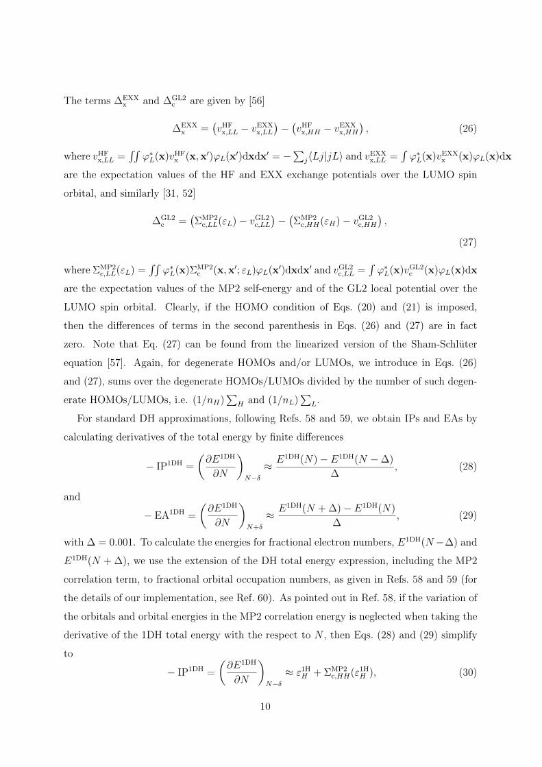
The terms ∆EXXx and ∆GL2
c are given by [56]
∆EXXx =
(vHFx,LL − vEXX
x,LL
)−(vHFx,HH − vEXX
x,HH
), (26)
where vHFx,LL =
∫∫ϕ∗L(x)vHF
x (x,x′)ϕL(x′)dxdx′ = −∑j〈Lj|jL〉 and vEXXx,LL =
∫ϕ∗L(x)vEXX
x (x)ϕL(x)dx
are the expectation values of the HF and EXX exchange potentials over the LUMO spin
orbital, and similarly [31, 52]
∆GL2c =
(ΣMP2
c,LL(εL)− vGL2c,LL
)−(ΣMP2
c,HH(εH)− vGL2c,HH
),
(27)
where ΣMP2c,LL(εL) =
∫∫ϕ∗L(x)ΣMP2
c (x,x′; εL)ϕL(x′)dxdx′ and vGL2c,LL =
∫ϕ∗L(x)vGL2
c (x)ϕL(x)dx
are the expectation values of the MP2 self-energy and of the GL2 local potential over the
LUMO spin orbital. Clearly, if the HOMO condition of Eqs. (20) and (21) is imposed,
then the differences of terms in the second parenthesis in Eqs. (26) and (27) are in fact
zero. Note that Eq. (27) can be found from the linearized version of the Sham-Schluter
equation [57]. Again, for degenerate HOMOs and/or LUMOs, we introduce in Eqs. (26)
and (27), sums over the degenerate HOMOs/LUMOs divided by the number of such degen-
erate HOMOs/LUMOs, i.e. (1/nH)∑
H and (1/nL)∑
L.
For standard DH approximations, following Refs. 58 and 59, we obtain IPs and EAs by
calculating derivatives of the total energy by finite differences
− IP1DH =
(∂E1DH
∂N
)
N−δ≈ E1DH(N)− E1DH(N −∆)
∆, (28)
and
− EA1DH =
(∂E1DH
∂N
)
N+δ
≈ E1DH(N + ∆)− E1DH(N)
∆, (29)
with ∆ = 0.001. To calculate the energies for fractional electron numbers, E1DH(N−∆) and
E1DH(N + ∆), we use the extension of the DH total energy expression, including the MP2
correlation term, to fractional orbital occupation numbers, as given in Refs. 58 and 59 (for
the details of our implementation, see Ref. 60). As pointed out in Ref. 58, if the variation of
the orbitals and orbital energies in the MP2 correlation energy is neglected when taking the
derivative of the 1DH total energy with the respect to N , then Eqs. (28) and (29) simplify
to
− IP1DH =
(∂E1DH
∂N
)
N−δ≈ ε1HH + ΣMP2
c,HH(ε1HH ), (30)
10

-2
-1.5
-1
-0.5
0
0 1 2 3 4 5 6
vxc (
hart
ree)
r (bohr)
Be
TSVD 10-4
TSVD 10-6
TSVD 10-8
-0.3
-0.25
-0.2
-0.15
-0.1
-0.05
0
0 1 2 3 4 5 6
vc (
hart
ree)
r (bohr)
Be
TSVD 10-4
TSVD 10-6
TSVD 10-8
-2
-1.5
-1
-0.5
0
-6 -4 -2 0 2 4 6
vxc (
hart
ree)
r (bohr)
CO
TSVD 10-4
TSVD 10-6
TSVD 10-8
-0.2
-0.15
-0.1
-0.05
0
0.05
0.1
0.15
0.2
0.25
-6 -4 -2 0 2 4 6
vc (
hart
ree)
r (bohr)
CO
TSVD 10-4
TSVD 10-6
TSVD 10-8
FIG. 1. Exchange-correlation and correlation potentials calculated with the OEP-1DH approx-
imation using the BLYP functional at the recommended value λ = 0.65 for the Be atom and
the CO molecule using different TSVD cutoffs 10−4, 10−6, 10−8 for the pseudo-inversion of the
linear-response function. For Be, the potentials for 10−4 and 10−6 are superimposed. For CO, the
potentials for 10−6 and 10−8 are superimposed.
and
− EA1DH =
(∂E1DH
∂N
)
N+δ
≈ ε1HL + ΣMP2c,LL(ε1HL ), (31)
which corresponds to standard second-order perturbative propagator theory (see, e.g.,
Ref. 49). Even though in practice we calculate IP1DH and EA1DH using Eqs. (28) and (29),
the approximate connection with the self-energy in Eqs. (30) and (31) is useful for compar-
ison and interpretative purposes. For example, it can be shown that ΣMP2c,HH(ε1HH ) contains a
term corresponding to orbital relaxation in the (N−1)-electron system, and pair-correlation
terms for the N - and (N − 1)-electron systems [49, 61].
III. COMPUTATIONAL DETAILS
The 1DH calculations have been performed with a development version of MOLPRO
2015 [62], and the OEP-1DH ones with a development version of ACES II [63]. In all
calculations, we have used the B exchange [23] and the LYP correlation [24] density func-
11

tionals, for EDFAx and EDFA
c , respectively. This choice was motivated by the fact that
1DH-BLYP was found to be among the one-parameter double-hybrid approximations giving
the most accurate thermochemistry properties on average [22, 28, 64]. We expect however
that the effect of the OEP self consistency to be similar when using other density func-
tional approximations. The performance of both DH methods has been tested against a
few atomic (He, Be, Ne, and Ar) and molecular (CO and H2O) systems. For the latter, we
considered the following equilibrium geometries: for CO d(C–O) = 1.128A, and for H2O
d(H–O) = 0.959A and a(H–O–H) = 103.9. In all cases, core excitations were included in
the second-order correlation term.
In our OEP calculations, for convenience of implementation, the same basis set is used
for expanding both the orbitals and the exchange-correlation potential. To ensure that the
basis sets chosen were flexible enough for representation of orbitals and exchange-correlation
potentials, all basis sets were constructed by full uncontraction of basis sets originally devel-
oped for correlated calculations, as in Refs. 65 and 66. In particular, we employed an even
tempered 20s10p2d basis for He, and an uncontracted ROOS–ATZP basis [67] for Be and
Ne. For Ar, we used a modified basis set [68] which combines s and p basis functions from
the uncontracted ROOS–ATZP [67] with d and f functions coming from the uncontracted
aug–cc–pwCVQZ basis set [69]. In the case of both molecular systems, the uncontracted
cc–pVTZ basis set of Dunning [70] was employed. For all OEP calculations standard con-
vergence criteria were enforced, corresponding to maximum deviations in density-matrix
elements of 10−8. In practice, the use of the same basis set for expanding both the orbitals
and the exchange-correlation potential leads to the necessity of truncating the auxiliary func-
tion space by the TSVD method for constructing the pseudo-inverse of the linear-response
function. The convergence of the potentials with respect to the TSVD cutoff was studied.
Figure 1 shows the example of the convergence of the exchange-correlation and correlation
potentials of the Be atom and the CO molecule. For Be, the potentials obtained with
the 10−4 and 10−6 cutoffs are essentially identical, while for the 10−8 cutoff the exchange-
correlation potential has non-physical oscillations and the correlation potential diverges. For
CO, the potentials obtained with the 10−4 cutoff are significantly different from the poten-
tials obtained with the 10−6 cutoff, while no difference can be seen between the potentials
obtained with the 10−6 and 10−8 cutoffs. A cutoff of 10−6 was thus chosen for all systems
to achieve a compromise between convergence and numerical stability.
12

In order to assess the quality of the results obtained with the standard and OEP-based
DH methods, we considered several reference data. We used estimated exact total ener-
gies extracted from numerical calculations [71] for He, Be, Ne, Ar, and from quadratic
configuration-interaction calculations extrapolated to the complete basis set [72] for CO and
H2O. We also used reference data from coupled-cluster singles-doubles with perturbative
triples [CCSD(T)] [73–76] calculations performed with the same basis sets. In particular,
these CCSD(T) calculations yielded densities which were used as input for generating refer-
ence KS potentials by inversion of the KS equations [77, 78], using the computational setup
described in Refs. 65 and 66. We also used estimated exact total energies extracted from
numerical calculations [71] for He, Be, Ne, Ar, and from quadratic configuration-interaction
calculations extrapolated to the complete basis set [72] for CO and H2O.
IV. RESULTS AND DISCUSSION
A. Total energies
Figure 2 shows the total energy of each system as a function of λ calculated with the 1DH
and OEP-1DH approximations. For comparison, CCSD(T) total energies calculated with
the same basis sets and estimated exact total energies taken from Refs. 71 and 72 are also
reported. Note that the CCSD(T) total energies are significantly higher than the estimated
exact energies, which is mostly due to the incompleteness of the basis sets used. Since the
explicit density-functional contribution of the DH calculations does not suffer from this large
basis incompleteness error, we prefer to use as reference the estimated exact energies.
At λ = 0, both DH methods reduce to standard KS using the BLYP functional, which
tends to overestimate the total energy by about 3 to 30 mhartree, except for Be atom where it
is underestimated (which may be connected to the presence of an important static correlation
contribution in this system). At λ = 1, the 1DH approximation reduces to standard MP2
(with HF orbitals), while the OEP-1DH approximation reduces to OEP-GL2 (i.e., the same
MP2 total energy expression but with fully self-consistently optimized OEP orbitals) [18, 19].
Standard MP2 systematically underestimates the total energy on magnitude (up to more
than 100 mhartree for Ar) which is partly due to the missing correlation contribution beyond
second order and to the incompleteness of the basis sets used. On the opposite, OEP-GL2
13

-2.908
-2.906
-2.904
-2.902
-2.900
-2.898
-2.896
0 0.2 0.4 0.6 0.8 1
Eto
t (h
art
ree)
λ
He
Estimated exact
CCSD(T)
1DHOEP-1DH
-128.990
-128.980
-128.970
-128.960
-128.950
-128.940
-128.930
-128.920
-128.910
-128.900
-128.890
0 0.2 0.4 0.6 0.8 1
Eto
t (h
art
ree)
λ
Ne
Estimated exact
CCSD(T)
1DHOEP-1DH
-527.580
-527.560
-527.540
-527.520
-527.500
-527.480
-527.460
-527.440
-527.420
0 0.2 0.4 0.6 0.8 1
Eto
t (h
art
ree)
λ
Ar
Estimated exact
CCSD(T)
1DHOEP-1DH
-14.690
-14.685
-14.680
-14.675
-14.670
-14.665
-14.660
-14.655
-14.650
-14.645
-14.640
0 0.2 0.4 0.6 0.8 1
Eto
t (h
art
ree)
λ
Be
Estimated exact
CCSD(T)
1DHOEP-1DH
-113.550
-113.500
-113.450
-113.400
-113.350
-113.300
-113.250
-113.200
0 0.2 0.4 0.6 0.8 1
Eto
t (h
art
ree)
λ
CO
Estimated exact
CCSD(T)
1DHOEP-1DH
-76.520
-76.500
-76.480
-76.460
-76.440
-76.420
-76.400
-76.380
-76.360
0 0.2 0.4 0.6 0.8 1
Eto
t (h
art
ree)
λ
H2O
Estimated exact
CCSD(T)
1DHOEP-1DH
FIG. 2. Total energies calculated with the 1DH and OEP-1DH approximations with the BLYP
functional as a function of λ. As reference values, CCSD(T) total energies calculated with the
same basis sets are given, as well as estimated exact total energies taken from Ref. 71 for He, Be,
Ne, Ar, and from Ref. 72 for CO and H2O. The vertical lines correspond to λ = 0.65, i.e. the value
recommended for 1DH with the BLYP functional in Ref. 22. For Be, the OEP-1DH calculations
are unstable for λ > 0.86.
systematically gives too negative total energies, as already known [19, 25]. For example, for
CO the OEP-GL2 total energy is more than 150 mhartree too low. Note that for Be the
OEP-GL2 calculation is unstable, as already reported [19, 20, 79]. The fact that OEP-GL2
gives much more negative total energies than standard MP2 should be connected to the fact
that the HOMO-LUMO orbital energy gap is much smaller with OEP-GL2 orbitals than
with HF orbitals (see results in Sections IV B and IV C).
In between the extreme values λ = 0 and λ = 1, the 1DH and OEP-1DH approximation
give smooth total energy curves, which start to visually differ for λ & 0.2. Note that for
14

Be the OEP-1DH calculations are stable for λ ≤ 0.86. At λ = 0.65, which is the value
recommended in Ref. 22 for 1DH with the BLYP functional, both 1DH and OEP-1DH give
more accurate total energies than their respective λ = 1 limits (i.e., MP2 and OEP-GL2),
but do not perform necessarily better than the λ = 0 limit (KS BLYP). Depending on
the system considered, at λ = 0.65, the 1DH total energy is either more accurate or about
equally accurate than the OEP-1DH total energy. Thus, even though OEP-1DH provides an
important improvement over OEP-GL2, we conclude that the self-consistent optimization of
the orbitals in the 1DH approximation (i.e., going from 1DH to OEP-1DH) does not lead to
improved ground-state total energies for the few systems considered here. We expect that
a similar conclusion generally holds for ground-state energy differences such as atomization
energies, similarly to what has been found for the case of the hybrid approximations [80].
B. HOMO orbital energies and ionization potentials
Figure 3 reports, for each system, the HOMO orbital energy in the 1H approximation
[Eq. (6)] and minus the IPs in the 1DH [Eq. (28)] and OEP-1DH [Eq. (23)] approximations as
a function of λ. The reference IPs are from CCSD(T) calculations with the same basis sets.
The HOMO orbital energy in the 1H approximation represents the simplest approximation
to −IP available when doing a 1DH calculation. At λ = 0, the 1H approximation reduces
to standard KS with the BLYP functional, and we recover the well-known fact the HOMO
orbital energy is much too high (underestimating the IP by about 4 to 8 eV for the systems
considered here) with a semilocal DFA like BLYP, most likely due to the self-interaction error
in the exchange density functional. At λ = 1, the 1H approximation reduces to standard HF,
and in this case the HOMO orbital energy is a much better estimate of −IP, overestimating
the IP by about 1 eV except for Be where it is underestimated by about the same amount.
In between λ = 0 and λ = 1, the 1H HOMO orbital energy varies nearly linearly with λ,
which suggests that the λ-dependence is largely dominated by the exchange potential in
Eq. (7). At λ = 0.65, the 1H HOMO orbital energy is always higher than the reference −IP,
by about 1 or 2 eV depending on the system considered.
The IPs obtained with the 1DH method, i.e. taking into account the MP2 correlation
term, are smaller than the 1H IPs for all λ and all systems considered here, with the exception
of Be for which it is a bit larger. This is consistent with previous works which found that
15

-24
-22
-20
-18
-16
0 0.2 0.4 0.6 0.8 1
εH
OM
O o
r -I
P (
eV
)
λ
He
-IP CCSD(T)
εHOMO 1H
-IP 1DH
-IP=εHOMO OEP-1DH
-24
-23
-22
-21
-20
-19
-18
-17
-16
-15
-14
-13
0 0.2 0.4 0.6 0.8 1
εH
OM
O o
r -I
P (
eV
)
λ
Ne
-IP CCSD(T)
εHOMO 1H
-IP 1DH
-IP=εHOMO OEP-1DH
-17
-16
-15
-14
-13
-12
-11
-10
0 0.2 0.4 0.6 0.8 1
εH
OM
O o
r -I
P (
eV
)
λ
Ar
-IP CCSD(T)
εHOMO 1H
-IP 1DH
-IP=εHOMO OEP-1DH
-9.5
-9.0
-8.5
-8.0
-7.5
-7.0
-6.5
-6.0
-5.5
-5.0
0 0.2 0.4 0.6 0.8 1
εH
OM
O o
r -I
P (
eV
)
λ
Be
-IP CCSD(T)
εHOMO 1H
-IP 1DH
-IP=εHOMO OEP-1DH
-16
-15
-14
-13
-12
-11
-10
-9
-8
0 0.2 0.4 0.6 0.8 1
εH
OM
O o
r -I
P (
eV
)
λ
CO
-IP CCSD(T)
εHOMO 1H
-IP 1DH
-IP=εHOMO OEP-1DH
-14
-13
-12
-11
-10
-9
-8
-7
-6
0 0.2 0.4 0.6 0.8 1
εH
OM
O o
r -I
P (
eV
)
λ
H2O
-IP CCSD(T)
εHOMO 1H
-IP 1DH
-IP=εHOMO OEP-1DH
FIG. 3. HOMO orbital energies in the 1H approximation [Eq. (6)] and minus IPs in the 1DH
[Eq. (28)] and OEP-1DH [Eq. (23)] approximations using the BLYP functional as a function of λ.
The reference values were calculated as CCSD(T) total energy differences with the same basis sets.
The vertical lines correspond to λ = 0.65, i.e. the value recommended for 1DH with the BLYP
functional in Ref. 22. For Be, the OEP-1DH calculations are unstable for λ > 0.86.
IPs calculating by taking the derivative of the MP2 total energy with respect the electron
number are generally too small [58, 81]. At λ = 0.65, 1DH gives IPs that are underestimated
by about 2 or 3 eV, which is similar to the average accuracy obtained with the two-parameter
B2-PLYP double-hybrid approximation [59]. The effect of self-consistency, i.e. going from
1DH to OEP-1DH, is to further reduce the IPs, except for Be for which it increases it. For
He the differences between 1DH and OEP-1DH are very small, which may not be surprising
since for such a two-electron system the HF and EXX potentials have the same action on
occupied orbitals. At λ = 1, OEP-GL2 gives IPs which are generally not very accurate
(see also Ref. 82). In particular, for Ne, CO, and H2O, OEP-GL2 underestimates the IP
16

-4
-2
0
2
4
6
0 0.2 0.4 0.6 0.8 1
εL
UM
O o
r -E
A (
eV
)
λ
He
-EA CCSD(T)
εLUMO KS[CCSD(T)]
εLUMO 1H
-EA 1DH
εLUMO OEP-1DH
-EA=εLUMO+∆xc OEP-1DH
-4
-2
0
2
4
6
0 0.2 0.4 0.6 0.8 1
εL
UM
O o
r -E
A (
eV
)
λ
Ne
-EA CCSD(T)
εLUMO KS[CCSD(T)]
εLUMO 1H
-EA 1DH
εLUMO OEP-1DH
-EA=εLUMO+∆xc OEP-1DH
-5
-4
-3
-2
-1
0
1
2
3
0 0.2 0.4 0.6 0.8 1
εL
UM
O o
r -E
A (
eV
)
λ
Ar
-EA CCSD(T)
εLUMO KS[CCSD(T)]
εLUMO 1H
-EA 1DH
εLUMO OEP-1DH
-EA=εLUMO+∆xc OEP-1DH
-6
-5
-4
-3
-2
-1
0
1
2
0 0.2 0.4 0.6 0.8 1
εL
UM
O o
r -E
A (
eV
)
λ
Be
-EA CCSD(T)
εLUMO KS[CCSD(T)]
εLUMO 1H
-EA 1DH
εLUMO OEP-1DH
-EA=εLUMO+∆xc OEP-1DH
-8
-6
-4
-2
0
2
4
6
8
0 0.2 0.4 0.6 0.8 1
εL
UM
O o
r -E
A (
eV
)
λ
CO
-EA CCSD(T)
εLUMO KS[CCSD(T)]
εLUMO 1H
-EA 1DH
εLUMO OEP-1DH
-EA=εLUMO+∆xc OEP-1DH
-4
-2
0
2
4
6
8
0 0.2 0.4 0.6 0.8 1
εL
UM
O o
r -E
A (
eV
)
λ
H2O
-EA CCSD(T)
εLUMO KS[CCSD(T)]
εLUMO 1H
-EA 1DH
εLUMO OEP-1DH
-EA=εLUMO+∆xc OEP-1DH
FIG. 4. LUMO orbital energies in the 1H [Eq. (6)] and OEP-1DH [Eq. (8)] approximations and mi-
nus EAs in the 1DH [Eq. (29)] and OEP-1DH [Eq. (24)] approximations using the BLYP functional
as a function of λ. The reference EA values were calculated as CCSD(T) total energy differences
with the same basis sets, and the reference HOMO energy values were calculated by KS inversion
of the CCSD(T) densities. The vertical lines correspond to λ = 0.65, i.e. the value recommended
for 1DH with the BLYP functional in Ref. 22. For Be, the OEP-1DH calculations are unstable for
λ > 0.86.
by more than 3 eV. As a consequence, for these systems, for λ & 0.5 self-consistency only
deteriorates the accuracy of the IPs. We note that better IPs could be obtained using
modified second-order correlated OEP approximations [82].
17

C. LUMO orbital energies and electronic affinities
Figure 4 reports, for each system, the LUMO orbital energy in the 1H [Eq. (6)] and
OEP-1DH [Eq. (8)] approximations and minus the EAs in the 1DH [Eq. (29)] and OEP-
1DH [Eq. (24), i.e. including the derivative discontinuity] approximations as a function of
λ. The reference EAs are from CCSD(T) calculations with the same basis sets, whereas the
reference KS LUMO orbital energies have been obtained by inversion of the KS equations
using CCSD(T) densities as input. The reference −EAs are all positive for the systems
considered, meaning that the anions are unstable. These positive values are an artifact of
the incompleteness of the basis set. In a complete basis set, the EAs should be either negative
(i.e., the anion is more stable than the neutral system) or zero (i.e., the anion dissociates into
the neutral system and a free electron). Even though the reported EA values are thus not
converged with respect to the basis set, the EAs given by different methods can nevertheless
be compared for a fixed basis set. By contrast, the reference KS LUMO orbital energies
are all correctly negative with the basis set employed. This is due to the fact that the KS
LUMO does not represent a state with an additional electron but a bound excited state of
the neutral system, which requires much less diffuse basis functions to describe. We note
however that, in the case of the CO and H2O molecules, the reported KS LUMO orbital
energies are not well converged with respect to the basis set due to the lack of diffuse basis
functions. Again, we can nevertheless meaningfully compare them with the reference data
obtained with the same basis sets.
The LUMO orbital energy in the 1H approximation represents the simplest approximation
to −EA (and not to the KS LUMO orbital energy since it is obtained with the nonlocal HF
potential) available when doing a 1DH calculation. At λ = 0, the 1H approximation reduces
to standard KS with the BLYP functional, and we recover the fact that LUMO orbital
energy with a semilocal DFA like BLYP is roughly half way between the exact KS LUMO
orbital energy and the exact −EA (i.e., εDFAL ≈ εexactL + ∆xc/2, see e.g. Ref. 83). At λ = 1,
the 1H approximation reduces to standard HF, and in this case the LUMO orbital energy is
a quite good estimate of −EA (within the finite basis set) for the systems considered here.
At λ = 0.65, the 1H LUMO orbital energy underestimates −EA by about 0.25 to 1 eV,
depending on the system.
The 1DH approximation gives −EAs rather close to the 1H ones, which indicates that
18

the MP2 correlation term has only a modest effect on this quantity for the systems consid-
ered. Coming now to the OEP-1DH results, the LUMO orbital energy obtained in these
calculations has a behavior as a function of λ which is clearly distinct from the other curves.
Starting from the BLYP LUMO orbital energy value at λ = 0, it becomes more negative as
λ is increased, and becomes an increasingly accurate approximation to the exact KS LUMO
orbital energy (and not to −EA). This is an essential difference between having a local
EXX (and GL2) potential instead of a nonlocal HF potential. At λ = 0.65, the OEP-1DH
LUMO orbital energies underestimate the reference KS LUMO energies by about 1 to 2 eV.
The estimate of −EA in the OEP-1DH approximation is obtained by adding the derivative
discontinuity ∆xc to the OEP-1DH LUMO orbital energy. For the closed-shell systems con-
sidered here, the derivative discontinuity is largely dominated by the exchange contribution.
The derivative discontinuity is systematically overestimated in OEP-GL2, leading to −EAs
that are much too high. It turns out that, at the recommended value λ = 0.65, OEP-1DH
gives −EAs which agree with the reference values within 0.4 eV for the systems considered.
Thus, the OEP-based self-consistency improves the accuracy of EAs.
D. Exchange-correlation and correlation potentials
Figure 5 shows the exchange-correlation potentials calculated by OEP-1DH at the rec-
ommended value of λ = 0.65, as well as the potentials obtained at the extreme values of λ,
corresponding to KS BLYP (λ = 0) and OEP-GL2 (λ = 1). The reference potentials have
been obtained by employing the KS inversion approach using the CCSD(T) densities.
The BLYP exchange-correlation potentials are not negative enough, they do not describe
well the shell structure (core/valence transition), and decay too fast at large distances. The
OEP-GL2 exchange-correlation potentials have the correct −1/r asymptotic behavior and
are quite accurate for the rare-gas atoms (especially for He and Ar), but have too much
structure for CO and H2O. For Be, the OEP-GL2 calculation is unstable. The OEP-1DH
exchange-correlation potentials do not have quite the correct asymptotic behavior since
they decay as −λ/r, but for λ = 0.65 they have reasonable shapes in the physically relevant
region of space. Note in particular that the OEP-1DH calculation yields a stable solution
for Be. For CO and H2O, the OEP-1DH exchange-correlation potentials actually improve
over both the BLYP and OEP-GL2 exchange-correlation potentials. Therefore, even though
19
-2
-1.5
-1
-0.5
0
0 1 2 3 4 5 6
vxc (
hart
ree)
r (bohr)
He
BLYPOEP-1DH (λ=0.65)
OEP-GL2KS [CCSD(T)]
-2
-1.5
-1
-0.5
0
0 1 2 3 4 5 6
vxc (
hart
ree)
r (bohr)
Ne
BLYPOEP-1DH (λ=0.65)
OEP-GL2KS [CCSD(T)]
-1.8
-1.6
-1.4
-1.2
-1
-0.8
-0.6
-0.4
-0.2
0
0 1 2 3 4 5 6
vxc (
hart
ree)
r (bohr)
Ar
BLYPOEP-1DH (λ=0.65)
OEP-GL2KS [CCSD(T)]
-2
-1.5
-1
-0.5
0
0 1 2 3 4 5 6
vxc (
hart
ree)
r (bohr)
Be
BLYPOEP-1DH (λ=0.65)
KS [CCSD(T)]
-2
-1.5
-1
-0.5
0
-6 -4 -2 0 2 4 6
vxc (
hart
ree)
r (bohr)
CO
BLYPOEP-1DH (λ=0.65)
OEP-GL2KS [CCSD(T)]
-2
-1.5
-1
-0.5
0
-6 -4 -2 0 2 4 6
vxc (
hart
ree)
r (bohr)
H2O
BLYPOEP-1DH (λ=0.65)
OEP-GL2KS [CCSD(T)]
FIG. 5. Exchange-correlation potentials calculated with the OEP-1DH approximation [Eq. (9)]
using the BLYP functional at the recommended value λ = 0.65, and at the extreme values λ = 0
(standard BLYP) and λ = 1 (OEP-GL2). The reference potentials were calculated by KS inversion
of the CCSD(T) densities. For Be, the OEP-GL2 calculations are unstable. For CO, the potential
is plotted along the direction of the bond with the C nucleus at −1.21790 bohr and the O nucleus
at 0.91371 bohr. For H2O, the potential is plotted along the direction of a OH bond with the O
nucleus at 0.0 and the H nucleus at 1.81225 bohr.
the recommended value of λ = 0.65 was determined based on energetical properties of the
standard non-self-consistent 1DH scheme, it appears that this value of λ also gives reasonable
exchange-correlation potentials as well.
The correlation part of the potentials are plotted in Figure 6. The correlation potentials
in BLYP calculations (i.e., the LYP correlation potential evaluated at the self-consistent
BLYP density) are unable to reproduce the complex structure of the reference correlation
potentials. Note that this is in spite of the fact that LYP correlation energies are usu-
20

-0.06
-0.04
-0.02
0
0.02
0.04
0 1 2 3 4 5 6
vc (
hart
ree)
r (bohr)
He
BLYPOEP-1DH (λ=0.65)
OEP-GL2KS [CCSD(T)]
-0.05
0
0.05
0.1
0.15
0.2
0.25
0.3
0.35
0 1 2 3 4 5 6
vc (
hart
ree)
r (bohr)
Ne
BLYPOEP-1DH (λ=0.65)
OEP-GL2KS [CCSD(T)]
-0.15
-0.1
-0.05
0
0.05
0 1 2 3 4 5 6
vc (
hart
ree)
r (bohr)
Ar
BLYPOEP-1DH (λ=0.65)
OEP-GL2KS [CCSD(T)]
-0.3
-0.25
-0.2
-0.15
-0.1
-0.05
0
0 1 2 3 4 5 6
vc (
hart
ree)
r (bohr)
Be
BLYPOEP-1DH (λ=0.65)
KS [CCSD(T)]
-0.2
-0.15
-0.1
-0.05
0
0.05
0.1
0.15
0.2
0.25
-6 -4 -2 0 2 4 6
vc (
hart
ree)
r (bohr)
CO BLYPOEP-1DH (λ=0.65)
OEP-GL2KS [CCSD(T)]
-0.3
-0.2
-0.1
0
0.1
-6 -4 -2 0 2 4 6
vc (
hart
ree)
r (bohr)
H2O
BLYPOEP-1DH (λ=0.65)
OEP-GL2KS [CCSD(T)]
FIG. 6. Correlation potentials calculated with the OEP-1DH approximation [correlation terms in
Eq. (9)] using the BLYP functional at the recommended value λ = 0.65, and at the extreme values
λ = 0 (standard BLYP) and λ = 1 (OEP-GL2). The reference potentials were calculated by KS
inversion of the CCSD(T) densities. For Be, the OEP-GL2 calculation is unstable. For CO, the
potential is plotted along the direction of the bond with the C nucleus at −1.21790 bohr and the
O nucleus at 0.91371 bohr. For H2O, the potential is plotted along the direction of a OH bond
with the O nucleus at 0.0 and the H nucleus at 1.81225 bohr.
ally reasonably accurate. On the contrary, the OEP-GL2 correlation potentials tend to be
largely overestimated, as previously observed [27, 65]. Overall, the OEP-1DH correlation
potentials at λ = 0.65 have fairly reasonable shapes, providing a good compromise between
the understructured BLYP and the overestimated OEP-GL2 correlation potentials.
21

-0.01
-0.005
0
0.005
0.01
0 0.5 1 1.5 2 2.5 3 3.5 4
4 π
r2 ∆
nc (
bo
hr-1
)
r (bohr)
He
BLYPOEP-1DH (λ=0.65)
MP2OEP-GL2CCSD(T)
-0.2
-0.15
-0.1
-0.05
0
0.05
0.1
0 0.5 1 1.5 2 2.5 3 3.5 4
4 π
r2 ∆
nc (b
oh
r-1)
r (bohr)
Ne
BLYPOEP-1DH (λ=0.65)
MP2OEP-GL2CCSD(T)
-0.06
-0.04
-0.02
0
0.02
0.04
0.06
0.08
0.1
0 0.5 1 1.5 2 2.5 3 3.5 4
4 π
r2 ∆
nc (
bo
hr-1
)
r (bohr)
Ar
BLYPOEP-1DH (λ=0.65)
MP2OEP-GL2CCSD(T)
-0.02
-0.01
0
0.01
0.02
0.03
0.04
0 1 2 3 4 5 6
4 π
r2 ∆
nc (
bo
hr-1
)
r (bohr)
Be
BLYPOEP-1DH (λ=0.65)
MP2CCSD(T)
-0.15
-0.1
-0.05
0
0.05
0.1
0.15
-3 -2 -1 0 1 2 3
∆n
c (
bo
hr-3
)
r (bohr)
CO
BLYP
OEP-1DH (λ=0.65)
MP2
OEP-GL2
CCSD(T)
-0.04
-0.02
0
0.02
0.04
0.06
-1 -0.5 0 0.5 1 1.5 2
∆n
c (
bo
hr-3
)
r (bohr)
H2OBLYP
OEP-1DH (λ=0.65)MP2
OEP-GL2CCSD(T)
FIG. 7. Correlated density calculated with the OEP-1DH approximation using the BLYP func-
tional at the recommended value λ = 0.65, and at the extreme values λ = 0 (standard BLYP)
and λ = 1 (OEP-GL2). The reference correlated densities are calculated with CCSD(T). For com-
parison, correlated densities calculated with standard MP2 are also shown. For Be, the OEP-GL2
calculation is unstable. For CO, the potential is plotted along the direction of the bond with the
C nucleus at −1.21790 bohr and the O nucleus at 0.91371 bohr. For H2O, the potential is plotted
along the direction of a OH bond with the O nucleus at 0.0 and the H nucleus at 1.81225 bohr.
E. Correlated densities
The analysis of the correlated densities provides a useful tool for the detailed examination
of the correlation effects on the electronic density and for the test of exchange-correlation
approximations in DFT [65, 66, 84–87]. Thus, in Figure 7 we report correlated densities
calculated by OEP-1DH at the recommended value of λ = 0.65, as well as the correlated
densities obtained at the extreme values of λ, corresponding to KS BLYP (λ = 0) and OEP-
22

GL2 (λ = 1). The correlated density is defined as ∆nc(r) = n(r) − nx-only(r) where n(r) is
the total density calculated with the full exchange and correlation terms and nx-only(r) is the
density calculated with only the exchange terms (see Refs. 65, 66, 84, and 85 for discussions
on different definitions of correlated densities). The reference correlated densities have been
calculated with the CCSD(T) method as ∆nc,CCSD(T)(r) = nCCSD(T)(r) − nHF(r), while
nCCSD(T)(r) was obtained from the CCSD(T) relaxed density matrix [88–90] constructed
using the Lagrangian approach [91–93]. For comparison, correlated densities calculated in
standard MP2 (1DH with λ = 1) with the same relaxed density-matrix approach are also
shown. Due to our current implementation limitations (lack of the relaxed density-matrix
approach for the 1DH approximation), the correlated densities for the non-self-consistent
1DH approximation have not been calculated.
At λ = 0, i.e. in KS BLYP calculations, the correlated densities are mostly very much
underestimated. At λ = 1, the correlated densities are largely overestimated with OEP-
GL2. At λ = 0.65, the OEP-1DH correlated densities tend to be quite accurate, achieving
a good balance between the underestimated BLYP correlated densities at λ = 0 and the
overestimated OEP-GL2 correlated densities at λ = 1. The OEP-1DH correlated densities
are overall similar in accuracy to the MP2 and CCSD(T) correlated densities.
V. CONCLUSION
In this work, we have proposed an OEP-based self-consistent DH scheme in which the or-
bitals are optimized with a local potential including the MP2 correlation contribution. While
staying in the philosophy of the KS scheme with a local potential, this scheme constitutes
an alternative to the orbital-optimized DH scheme of Peverati and Head-Gordon [7].
We have implemented a one-parameter version of this OEP-based self-consistent DH
scheme using the BLYP density-functional approximation and compared it to the corre-
sponding non-self-consistent DH scheme for calculations on a few closed-shell atoms and
molecules. While the OEP-based self-consistency does not provide any improvement for the
calculations of ground-state total energies and ionization potentials, it does improve the accu-
racy of electron affinities and restores the meaning of the LUMO orbital energy as being con-
nected to a neutral excitation energy. Moreover, the OEP-based self-consistent DH scheme
provides reasonably accurate exchange-correlation potentials and correlated densities. In
23

comparison to the standard OEP-GL2 method [16–20], our OEP-based self-consistent DH
scheme is more stable and removes the large overestimation of correlation effects.
Additional work can be foreseen to exploit the full power of the OEP-based self-consistent
DH scheme. For example, our scheme should be tested against more systems, including open-
shell ones for which we expect the OEP self-consistency to provide advantages similar to
the orbital-optimized DH scheme of Ref. 7. It would also be interesting to apply linear-
response time-dependent DFT on our OEP-based self-consistent DH scheme to calculate
excitation energies. Finally, the present procedure should be applied to the range-separated
DH approach [94] which has the advantage of having a fast basis convergence [95].
ACKNOWLEDGEMENTS
We thank Andreas Savin for discussions, as well as Andrew Teale for providing the
reference data for the exchange and exchange-correlation potentials. This work was
supported by French state funds managed by CALSIMLAB, within the Investissements
d’Avenir program under reference ANR-11-IDEX-0004-02, by the Polish-French bilateral
programme POLONIUM, and by the Polish National Science Center under Grant No.
DEC-2013/11/B/ST4/00771.
[1] P. Hohenberg and W. Kohn, Phys. Rev. 136, B 864 (1964).
[2] W. Kohn and L. J. Sham, Phys. Rev. 140, A1133 (1965).
[3] A. D. Becke, J. Chem. Phys. 140, 18A301 (2014).
[4] S. Grimme, J. Chem. Phys. 124, 034108 (2006).
[5] L. Goerigk and S. Grimme, WIREs Comput. Mol. Sci. 4, 576 (2014).
[6] A. Seidl, A. Gorling, P. Vogl, J. A. Majewski, and M. Levy, Phys. Rev. B 53, 3764 (1996).
[7] R. Peverati and M. Head-Gordon, J. Chem. Phys. 139, 024110 (2013).
[8] R. C. Lochan and M. Head-Gordon, J. Chem. Phys. 126, 164101 (2007).
[9] F. Neese, T. Schwabe, S. Kossmann, B. Schirmer, and S. Grimme, J. Chem. Theory Comput.
5, 3060 (2009).
24

[10] J. C. Sancho-Garcıa, A. J. Perez-Jimenez, M. Savarese, E. Bremond, and C. Adamo, J. Phys.
Chem. A 120, 1756 (2016).
[11] R. T. Sharp and G. K. Horton, Phys. Rev. 90, 317 (1953).
[12] J. D. Talman and W. F. Shadwick, Phys. Rev. A 14, 36 (1976).
[13] T. Grabo, T. Kreibich, S. Kurth, and E. K. U. Gross, in Strong Coulomb Correlation in Elec-
tronic Structure: Beyond the Local Density Approximation, edited by V. Anisimov (Gordon
& Breach, Tokyo, 2000).
[14] E. Engel, in A Primer in Density Functional Theory, Vol. 620 of Lecture Notes in Physics,
edited by C. Fiolhais, F. Nogueira, and M. A. L. Marques (Springer, Berlin, 2003) pp. 56–122.
[15] S. Kummel and L. Kronik, Rev. Mod. Phys. 80, 3 (2008).
[16] A. Gorling and M. Levy, Phys. Rev. A 50, 196 (1994).
[17] A. Gorling and M. Levy, Int. J. Quantum Chem. Symp. 29, 93 (1995).
[18] I. Grabowski, S. Hirata, S. Ivanov, and R. J. Bartlett, J. Chem. Phys. 116, 4415 (2002).
[19] R. J. Bartlett, I. Grabowski, S. Hirata, and S. Ivanov, J. Chem. Phys. 122, 034104 (2005).
[20] P. Mori-Sanchez, Q. Wu, and W. Yang, J. Chem. Phys. 123, 062204 (2005).
[21] S. Hirata, S. Ivanov, I. Grabowski, and R. J. Bartlett, J. Chem. Phys. 116, 6468 (2002).
[22] K. Sharkas, J. Toulouse, and A. Savin, J. Chem. Phys. 134, 064113 (2011).
[23] A. D. Becke, Phys. Rev. A 38, 3098 (1988).
[24] C. Lee, W. Yang, and R. G. Parr, Phys. Rev. B 37, 785 (1988).
[25] I. Grabowski, V. Lotrich, and R. J. Bartlett, J. Chem. Phys. 127, 154111 (2007).
[26] I. Grabowski, Int. J. Quantum Chem. 108, 2076 (2008).
[27] I. Grabowski, E. Fabiano, A. M. Teale, S. Smiga, A. Buksztel, and F. Della Salla, J. Chem.
Phys. 141, 024113 (2014).
[28] S. M. O. Souvi, K. Sharkas, and J. Toulouse, J. Chem. Phys. 140, 084107 (2014).
[29] K. Sharkas, J. Toulouse, L. Maschio, and B. Civalleri, J. Chem. Phys. 141, 044105 (2014).
[30] J. B. Krieger, Y. Li, and G. J. Iafrate, Phys. Rev. A 46, 5453 (1992).
[31] M. E. Casida, Phys. Rev. A 51, 2005 (1995).
[32] F. Della Salla and A. Gorling, J. Chem. Phys. 115, 5718 (2001).
[33] M. Gruning, O. V. Gritsenko, and E. J. Baerends, J. Chem. Phys. 116, 6435 (2002).
[34] A. Heßelmann, J. Chem. Phys. 8, 563 (2006).
[35] E. Fabiano and F. Della Sala, J. Chem. Phys. 126, 214102 (2007).
25

[36] A. F. Izmaylov, V. N. Staroverov, G. E. Scuseria, and E. R. Davidson, J. Chem. Phys. 127,
084113 (2007).
[37] E. Engel and R. M. Dreizler, J. Comput. Chem. 20, 31 (1999).
[38] S. Ivanov, S. Hirata, and R. J. Bartlett, Phys. Rev. Lett. 83, 5455 (1999).
[39] A. Gorling, Phys. Rev. Lett. 83, 5459 (1999).
[40] S. Hirata, S. Ivanov, I. Grabowski, R. J. Bartlett, K. Burke, and J. D. Talman, J. Chem.
Phys. 115, 1635 (2001).
[41] S. Ivanov, S. Hirata, and R. J. Bartlett, J. Chem. Phys. 116, 1269 (2002).
[42] W. Yang and Q. Wu, Phys. Rev. Lett. 89, 143002 (2002).
[43] A. Facco Bonetti, E. Engel, R. N. Schmid, and R. M. Dreizler, Phys. Rev. Lett. 86, 2241
(2001).
[44] Y. M. Niquet, M. Fuchs, and X. Gonze, Phys. Rev. Lett. 90, 219301 (2003).
[45] A. Facco Bonetti, E. Engel, R. N. Schmid, and R. M. Dreizler, Phys. Rev. Lett. 90, 219302
(2003).
[46] S. Ivanov and M. Levy, J. Chem. Phys. 116, 6924.
[47] E. Engel, H. Jiang, and A. Facco Bonetti, Phys. Rev. A 72, 052503 (2005).
[48] Y. M. Niquet, M. Fuchs, and X. Gonze, J. Chem. Phys. 118, 9504 (2003).
[49] A. Szabo and N. S. Ostlund, Modern Quantum Chemistry: Introduction to Advanced Electronic
Structure Theory (Dover, New York, 1996).
[50] J. B. Krieger, Y. Li, and G. J. Iafrate, Phys. Rev. A 45, 101 (1992).
[51] W. Yang, A. J. Cohen, and P. Mori-Sanchez, J. Chem. Phys. 136, 204111 (2012).
[52] M. E. Casida, Phys. Rev. B 59, 4694 (1999).
[53] A. Heßelmann, A. W. Gotz, F. Della Sala, and A. Gorling, J. Chem. Phys. 127, 054102 (2007).
[54] J. P. Perdew, R. G. Parr, M. Levy, and J. L. Balduz, Phys. Rev. Lett. 49, 1691 (1982).
[55] A. J. Cohen, P. Mori-Sanchez, and W. Yang, Phys. Rev. B 77, 115123 (2008).
[56] A. Gorling and M. Levy, Phys. Rev. A 52, 4493 (1995).
[57] L. J. Sham and M. Schluter, Phys. Rev. Lett. 51, 1888 (1983).
[58] A. J. Cohen, P. Mori-Sanchez, and W. Yang, J. Chem. Theory Comput. 5, 786 (2009).
[59] N. Q. Su, W. Yang, P. Mori-Sanchez, and X. Xu, J. Phys. Chem. A 118, 9201 (2014).
[60] B. Mussard and J. Toulouse, Fractional-charge and fractional-spin errors in
range-separated density-functional theory, Mol. Phys., published online (2016);
26

doi=10.1080/00268976.2016.1213910, preprint arXiv:1607.03621.
[61] B. T. Pickup and O. Goscinski, Mol. Phys. 26, 1013 (1973).
[62] H.-J. Werner, P. J. Knowles, G. Knizia, F. R. Manby, M. Schutz, and others, “MOLPRO,
version 2015.1, a package of ab initio programs,” Cardiff, UK, 2015, see http://www.molpro.
net.
[63] J. F. Stanton, J. Gauss, J. D. Watts, M. Nooijen, N. Oliphant, S. A. Perera, P. Szalay, W. J.
Lauderdale, S. Kucharski, S. Gwaltney, S. Beck, A. Balkova, D. E. Bernholdt, K. K. Baeck,
P. Rozyczko, H. Sekino, C. Hober, and R. J. Bartlett Integral packages included are VMOL
(J. Almlf and P.R. Taylor); VPROPS (P. Taylor) ABACUS; (T. Helgaker, H.J. Aa. Jensen,
P. Jorgensen, J. Olsen, and P.R. Taylor), ACES II (Quantum Theory Project, Gainesville,
Florida, 2007).
[64] J. Toulouse, K. Sharkas, E. Bremond, and C. Adamo, J. Chem. Phys. 135, 101102 (2011).
[65] I. Grabowski, A. M. Teale, S. Smiga, and R. J. Bartlett, J. Chem. Phys. 135, 114111 (2011).
[66] I. Grabowski, A. M. Teale, E. Fabiano, S. Smiga, A. Buksztel, and F. Della Sala, Mol. Phys.
112, 700 (2014).
[67] P. O. Widmark, P. A. Malmqvist, and B. Roos, Theor. Chim. Acta 77, 291 (1990).
[68] I. Grabowski, E. Fabiano, and F. Della Sala, Phys. Rev. B 87, 075103 (2013).
[69] K. A. Peterson and T. H. Dunning, Jr, J. Chem. Phys. 117, 10548 (2002).
[70] T. H. Dunning, Jr., J. Chem. Phys. 90, 1007 (1989).
[71] S. J. Chakravorty, S. R. Gwaltney, E. R. Davidson, F. A. Parpia, and C. F. Fischer, Phys.
Rev. A 47, 3649 (1993).
[72] W. Klopper, K. L. Bak, P. Jørgensen, J. Olsen, and T. Helgaker, J. Phys. B 32, R103 (1999).
[73] G. D. Purvis and R. J. Bartlett, J. Chem. Phys. 76, 1910 (1982).
[74] J. A. Pople, M. HeadGordon, and K. Raghavachari, J. Chem. Phys. 87, 5968 (1987).
[75] G. E. Scuseria, C. L. Janssen, and H. F. Schaefer, J. Chem. Phys. 89, 7382 (1988).
[76] K. Raghavachari, G. W. Trucks, J. A. Pople, and M. Head-Gordon, Chem. Phys. Lett. 157,
479 (1989).
[77] F. Colonna and A. Savin, J. Chem. Phys. 110, 2828 (1999).
[78] Q. Wu and W. Yang, J. Chem. Phys. 118, 2498 (2003).
[79] H. Jiang and E. Engel, J. Chem. Phys. 123, 224102 (2005).
[80] V. V. Karasiev, J. Chem. Phys. 118, 8576 (2003).
27

[81] N. Q. Su and X. Xu, J. Chem. Theory Comput. 11, 4677 (2015).
[82] S. Smiga, F. Della Salla, A. Buksztel, I. Grabowski, E. Fabiano, J. Comput. Chem. 37, 2081
(2016).
[83] A. M. Teale, F. De Proft, and D. Tozer, J. Chem. Phys. 129, 044110 (2008).
[84] K. Jankowski, K. Nowakowski, I. Grabowski, and J. Wasilewski, J. Chem. Phys. 130, 164102
(2009).
[85] K. Jankowski, K. Nowakowski, I. Grabowski, and J. Wasilewski, Theor. Chem. Acc. 125, 433
(2010).
[86] S. Smiga, A. Buksztel, and I. Grabowski, in Proceedings of MEST 2012: Electronic structure
methods with applications to experimental chemistry, Adv. Quantum Chem., Vol. 68, edited
by P. Hoggan (Academic Press, 2014) pp. 125 – 151.
[87] A. Buksztel, S. Smiga, and I. Grabowski, in Electron Correlation in Molecules ab initio
Beyond Gaussian Quantum Chemistry, Advances in Quantum Chemistry, Vol. 73, edited by
P. E. Hoggan and T. Ozdogan (Academic Press, 2016) pp. 263 – 283.
[88] N. C. Handy and H. F. Schaefer III, J. Chem. Phys. 81, 5031 (1984).
[89] J. E. Rice and R. D. Amos, Chem. Phys. Lett. 122, 585 (1985).
[90] E. A. Salter, G. W. Trucks, and R. J. Bartlett, J. Chem. Phys. 90, 1752 (1989).
[91] P. Jørgensen and T. Helgaker, J. Chem. Phys. 89, 1560 (1988).
[92] H. Koch, H. J. A. Jensen, P. Jørgensen, T. Helgaker, G. E. Scuseria, and H. F. Schaefer III,
J. Chem. Phys. 92, 4924 (1990).
[93] K. Hald, A. Halkier, P. Jørgensen, S. Coriani, C. Hattig, and T. Helgaker, J. Chem. Phys.
118, 2985 (2003).
[94] J. G. Angyan, I. C. Gerber, A. Savin, and J. Toulouse, Phys. Rev. A 72, 012510 (2005).
[95] O. Franck, B. Mussard, E. Luppi, and J. Toulouse, J. Chem. Phys. 142, 074107 (2015).
28

Chapter 4
Study of the short-range
exchange-correlation kernel
4.1 Introduction
Time-dependent density-functional theory (TDDFT) [1] and especially the linear-response
formalism is one of the most used approach for the calculation of electronic excitation ener-
gies. The key quantity in this context is the exchange-correlation kernel which is space and
frequency dependent and needs to be approximated. The frequency dependence is very difficult
to treat [2] and most of the time this dependence is neglected which is called the adiabatic
approximation. Most of the time a further approximation is made by using semilocal density
functionals. Despite this crude approximation adiabatic semilocal exchange-correlation kernels
give reasonably accurate results in many cases at low computational cost. However, adiabatic
semilocal approximations have some limitations: they give too low charge-transfer and Rydberg
excitation energies [3, 4], they fail to describe double excitations [5, 6] or to describe excitation
states along bond dissociations coordinates [7].
A way to overcome the limitations of the semilocal approximations is to extend TDDFT to
range separation [8]. The description of Rydberg and charge-transfer excitation energies can
be improved by introducing a long-range Hartree-Fock exchange kernel [9]. The long-range
correlation can be described using long-range linear-response density-matrix-functional theory
(DMFT) [10] or long-range linear-response multiconfigurational self-consistent field [11] that
give access to double excitations. In practice, in the range-separated TDDFT approaches the
short-range exchange-correlation kernel remains described by an adiabatic approximation.
In this study we considered linear-response TDDFT extended to range separation and we
studied in particular the frequency dependence of the short-range exchange-correlation kernel.
We were particularly interested by the behavior of the short-range exchange and correlation
79

80 CHAPTER 4. STUDY OF SHORT-RANGE EXCHANGE-CORRELATION KERNEL
kernels as a function of the range-separation parameter. The chapter is organized as follows.
A brief review of TDDFT is proposed in Sec. 4.2. The form of the exchange kernel is then
explored: the exact-exchange kernel is first generalized to range separation in Sec. 4.3 and
the asymptotic behavior of the short-range exact-exchange kernel with respect to the range-
separation parameter µ is studied in Sec. 4.4. Finally the form of the short-range correlation
kernel is explored in the special case of H2 in a minimal basis in Sec. 4.5.
4.2 Review on time-dependent density-functional theory
4.2.1 Time-dependent Schrodinger equation for many-electron systems
The time evolution of a N -particle system in a time-dependent external scalar potential is
described by the time-dependent Schrodinger equation that propagates a given initial state
Ψ(t0) = Ψ0
i∂
∂t|Ψ(t)〉 = H|Ψ(t)〉, (4.1)
with the N -particle Hamiltonian
H(t) = T + V (t) + Wee, (4.2)
with the kinetic operator T = −12
∫[∇2
rn1(r, r′)]r=r′dr, the electron-electron interaction Wee =12
∫∫n2(r, r′)/|r−r′|drdr′ and the time-dependent potential V (t) =
∫v(r, t)n(r)dr that contains
the contributions from the electron-nuclei interaction and the external electric-field perturbation.
In these expressions, n1(r, r′) is the one-particle density matrix operator, n2(r, r′) is the pair-
density operator and n(r) is the density operator.
The time-dependent many-body Schrodinger equation cannot be solved exactly for most of
molecular systems and approximated methods have to be used. One of the most widely used
method is time-dependent density-functional theory (TDDFT).
4.2.2 Time-dependent density-functional theory: the Kohn-Sham formalism
The fundamental statement of TDDFT is that the properties of the interacting system can
be deduced from the knowledge of the time-dependent density n(r, t) with a fixed initial state
condition. This is possible due to the Runge-Gross theorem [1] that can be considered as
an extension at the time-dependent level of the first Hohenberg-Kohn theorem. In the time-
dependent Kohn-Sham (KS) scheme the real system is replaced by a model system of non-
interacting particles
id
dt|ϕi(t)〉 =
[T + VKS[n](t)
]|ϕi(t)〉 (4.3)
with the same density as in the real system n(r, t) =∑occ.
i |ϕi(r, t)|2 and the Kohn-Sham
potential operator VKS[n](t) =∫n(r)vKS(r, t)dr. This density is imposed by the time-dependent

4.2. REVIEW ON TIME-DEPENDENT DENSITY-FUNCTIONAL THEORY 81
Kohn-Sham potential
vKS(r, t) = v(r, t) + vH(r, t) + vxc(r, t) (4.4)
with the time-dependent Hartree potential
vH(r, t) =
∫dr′
n(r′, t)|r− r′| (4.5)
and vxc(r, t) the time-dependent exchange-correlation potential that needs to be approximated.
The most common approximation is the adiabatic approximation.
The adiabatic approximation: In this approximation a functional defined for ground-state
DFT is used with a density that corresponds to the time-dependent density at fixed time. This
approximation is local in time
vadiabaticxc (r, t) =
δExc[n]
δn
∣∣∣∣n=n(r,t)
(4.6)
where Exc[n] is the ground-state exchange-correlation density functional.
4.2.3 Linear-response
If the time-dependent external potential is small enough it is not necessary to solve the time-
dependent Kohn-Sham equation. Calculating the linear change of the density allows us to
calculate linear-response properties such as the optical absorption spectrum.
While t < t0 the time-dependent external potential is switched off and the system is only subject
to the nuclear potential and is in its ground state. At t0 the time-dependent perturbation v(1)
is switched on and will induce a change in the density
n(r, t) = n(0)(r) + n(1)(r, t) + n(2)(r, t) + . . . (4.7)
the first-order term of the density depends linearly on v(1) and is sufficient to describe a weak
perturbation
n(1)(r, t) =
∫ t
t0
dt′∫
dr′χ(r, t; r′, t′)v(1)(r′, t′) (4.8)
with χ(r, t; r′, t′) the linear-response function of the system. The linear change can also be
expressed using the Kohn-Sham system
n(1)(r, t) =
∫ t
t0
dt′∫
dr′χ0(r, t; r′, t′)v(1)KS(r′, t′) (4.9)

82 CHAPTER 4. STUDY OF SHORT-RANGE EXCHANGE-CORRELATION KERNEL
with χ0(r, t; r′, t′) the Kohn-Sham linear-response function. The potential v(r, t) can be ex-
pressed with respect to the Kohn-Sham potential
v(r, t) = vKS(r, t)− vHxc(r, t) (4.10)
and can be differentiated with respect to the density
δv(r, t)
δn(r′, t′)=δvKS(r, t)
δn(r′, t′)− δvHxc(r, t)
δn(r′, t′)(4.11)
which can be expressed in frequency space
χ−1(r, r′, ω) = χ−10 (r, r′, ω)− fHxc(r, r
′, ω) (4.12)
with the Kohn-Sham linear-response function
χ0(r, r′, ω) =
occ.∑
i
unocc.∑
a
ϕ∗i (r)ϕa(r)ϕ∗a(r′)ϕi(r′)
εi − εa + ω + i0++
occ.∑
i
unocc.∑
a
ϕ∗a(r)ϕi(r)ϕ∗i (r′)ϕa(r′)
εi − εa − ω − i0+(4.13)
and fHxc the Hartree-exchange-correlation kernel that needs to be approximated.
4.2.4 Range-separated TDDFT
By decomposing the electron-electron interaction into long-range and short-range parts, the
many-electron system can alternatively be replaced by a long-range interacting effective system
id
dt|Ψlr(t)〉 =
[T + W lr
ee + V sr(t)]|Ψlr(t)〉, (4.14)
with the time-dependent long-range wave function Ψlr which gives the time-dependent density
equal to the density of the true system n(r, t). The short-range potential operator is V sr(t) =∫drn(r)vsr(r, t) with
vsr(r, t) = v(r, t) + vsrHxc(r, t) (4.15)
and in analogy with the previous section the linear-response theory can then be expressed as
χ−1(r, r′, ω) = (χlr)−1(r, r′, ω)− f srHxc(r, r
′, ω) (4.16)
with χlr the response function of the system described by the Hamiltonian in Eq. (4.14) and the
short-range Hartree-exchange-correlation kernel f srHxc(r, r
′, ω) that remains to approximate.

4.3. STUDY OF THE SHORT-RANGE EXCHANGE KERNEL 83
4.3 Study of the short-range exchange kernel
4.3.1 Range-separated time-dependent exact-exchange method
The time-dependent exact-exchange (TDEXX) method was introduced by Gorling [12, 13]. In
this section we extend this method to range separation by applying a perturbation theory along
the adiabatic connection following the derivation of Ref. [14]. The derivation will be restrained to
closed-shell systems. We first consider the range-separated time-dependent Schrodinger equation
id
dt|Ψlr,λ(t)〉 =
[T + V sr,λ(t) + λW lr
ee
]|Ψlr,λ(t)〉 (4.17)
with W lree the long-range electron-electron interaction and V sr,λ the potential operator keeping
the time-dependent density constant for every value of the coupling constant λ. The initial
condition Ψlr,λ(t0) is chosen to reproduce the initial density n(r, t0) for all λ. When λ = 0 the
system is the non-interacting system and can be described by the time-dependent Kohn-Sham
equation
id
dt|ΦKS(t)〉 =
[T + VKS(t)
]|ΦKS(t)〉 (4.18)
with the initial condition ΦKS(t0) = Ψlr,λ=0(t0) and the potential V sr,λ=0(t) = VKS(t) = V (t) +
VHxc(t). At λ = 1 the system is the partially interacting system described by the range-separated
time-dependent Schrodinger equation with the potential V sr,λ=1(t) = V (t)+ V srHxc(t). The short-
range potential is Taylor expanded with respect to λ
vsr,λ(r, t) =
∞∑
k=0
λkvsr,(k)(r, t) = vKS(r, t) + λvsr,(1)(r, t) + λ2vsr,(2)(r, t) + . . . (4.19)
The short-range potential can be written as
vsr,λ(r, t) = v(r, t) + vsr,λHxc(r, t) = vKS(r, t)−
(vHxc(r, t)− vsr,λ
Hxc(r, t)), (4.20)
the first-order contribution to the short-range potential is then
vsr,(1)(r, t) = −(vH(r, t)− vsrH(r, t))− (vx(r, t)− vsr
x (r, t)) = −vlrH(r, t)− vlr
x (r, t), (4.21)
with vsrH(r, t) and vsr
x (r, t) the short-range Hartree and exchange potentials and vlrH(r, t) and
vlrx (r, t) the long-range Hartree and exchange potentials. The dependence of the first-order
contribution to the short-range potential on the long-range Hartree and exchange potentials can
seem counter-intuitive but this can be explained by the long-range nature of the perturbation
introduced in Eq. (4.17). The sum of the remaining terms k ≥ 2 corresponds to the negative
of the long-range correlation potential. Considering the Taylor expansion of the potential in
Eq. (4.19) the Hamiltonian is written as

84 CHAPTER 4. STUDY OF SHORT-RANGE EXCHANGE-CORRELATION KERNEL
T + VKS(t) + λ[W lr
ee − V lrH (t)− V lr
x (t)]− λ2V lr,(2)(t) + . . . (4.22)
Then we expand the density with respect to λ,
nλ(r, t) =∞∑
k=0
λkn(k)(r, t), (4.23)
every term higher than the zeroth-order being zero because the density remains constant along
the adiabatic connection. To express the first-order contribution of the density we finally need
to expand the long-range wave function Ψlr(t) with respect to λ
Ψlr,λ(t) =
∞∑
k=0
λkΨlr,(k)(t) = ΦKS(t) + λΨlr,(1)(t) + λ2Ψlr,(2)(t) + . . . (4.24)
In the time-dependent case every Taylor expansion depends on the choice of the initial condition.
The initial-state wave function is chosen to be the ground state of a range-separated time-
independent Schrodinger equation Ψlr,λ(t0) = Ψlr,λ0
[T + U sr,λ + λW lr
ee
]|Ψlr,λ
0 〉 = Eλ0 |Ψlr,λ0 〉, (4.25)
with U sr,λ is the time-independent potential operator associated with the potential usr,λ(r) which
keeps the density constant along the adiabatic connection. At this point of the derivation the
time-dependent potential and the static potential do not need to be equal initially usr,λ(r) 6=vsr,λ(r, t0). The expansion of the wave-function in Eq. (4.24) becomes, for the initial state
Ψlr,λ0 =
∞∑
k=0
λkΨlr,(k)0 = ΦKS
0 + λΨlr,(1)0 + λ2Ψ
lr,(2)0 + . . . (4.26)
Time-dependent perturbation theory [12] yields the first-order contribution to the wave func-
tion Ψlr,λ(t) due to the first-order perturbation in Eq. (4.22)
Ψlr,(1)(t) = (−i)∞∑
k=0
ΦKSk (t)
∫ t
t0
dt′〈ΦKSk (t′)|W lr
ee − V lrH (t′)− V lr
x (t′)|ΦKS0 (t′)〉
+
∞∑
l=1
ΦKSl (t)
〈ΦKSl |W lr
ee − U lrH − U lr
x |ΦKS0 〉
EKS0 − EKS
l
, (4.27)
where ΦKSk (t) are the solutions from the time-dependent Kohn-Sham equation that evolve from
ΦKSk , the k-th eigenstate of the time-independent Kohn-Sham equation ΦKS
k (t0) = ΦKSk . The
first-order contribution to the density is then
n(1)(r, t) = 〈ΦKS0 (t)|n(r)|Ψlr,(1)(t)〉+ c.c.= 0, (4.28)

4.3. STUDY OF THE SHORT-RANGE EXCHANGE KERNEL 85
where ΦKS0 (t) is the zeroth-order term of Ψlr,λ(t) evolving from the initial condition ΦKS(t0) =
ΦKS0 . Combined to the expression of Ψlr,(1)(t) of Eq. (4.27) it becomes
0 =(−i)∞∑
k=0
〈ΦKS0 (t)|n(r)|ΦKS
k (t)〉∫ t
t0
dt′〈ΦKSk (t′)|W lr
ee − V lrH (t′)− V lr
x (t′)|ΦKS0 (t′)〉+ c.c.
+∞∑
l=1
〈ΦKS0 (t)|n(r)| ΦKS
l (t)〉〈ΦKSl |W lr
ee − U lrH − U lr
x |ΦKS0 〉
EKS0 − EKS
l
+ c.c.. (4.29)
The time-dependent and time-independent Kohn-Sham wave functions are Slater determinants
constructed from orbitals ϕk and ϕk(t) satisfying the time-independent and time-dependent
one-particle Kohn-Sham equations respectively
[T + UKS
]|ϕk〉 = εk|ϕk〉 (4.30)
id
dt|ϕk(t)〉 =
[T + VKS(t)
]|ϕk(t)〉. (4.31)
We can then express Eq. (4.29) with the Kohn-Sham orbitals and after some algebra we arrive
to the range-separated time-dependent exact-exchange equation
∫ t
t0
dt′∫
dr′χ0(r, t; r′, t′)vlrx (r′, t′) = Λlr
x (r, t) (4.32)
with the Kohn-Sham linear-response function
χ0(r, t; r′, t′) = 2(−i)occ.∑
i
unocc.∑
a
ϕ∗i (r, t)ϕa(r, t)ϕ∗a(r′, t′)ϕi(r′, t′) + c.c. (4.33)
and the right-hand side of Eq. (4.32)
Λlrx (r, t) =2(−i)
occ.∑
i
unocc.∑
a
ϕ∗i (r, t)ϕa(r, t)∫ t
t0
dt′〈ϕa(t′)|V NL,lrx (t′)|ϕi(t′)〉+ c.c. (4.34)
+ 2
occ.∑
i
unocc.∑
a
ϕ∗i (r, t)ϕa(r, t)×〈ϕa|UNL,lr
x − U lrx |ϕi〉
εi − εa+ c.c..
The factor 2 is due to the summation over the spin degree of freedom for closed-shell systems.
The non-local (NL) exchange potential corresponds to the Hartree-Fock exchange potential
applied to the Kohn-Sham orbitals
[V NL,lr
x (t)ϕk(t)]
(r) = −∫ occ.∑
j
ϕj(r, t)ϕ∗j (r′, t)ϕk(r
′, t)wlree(|r− r′|)dr′ (4.35)

86 CHAPTER 4. STUDY OF SHORT-RANGE EXCHANGE-CORRELATION KERNEL
and UNL,lrx and U lr
x are the time-independent long-range non-local and local exchange potentials,
respectively.
The short-range exchange potential can be obtained from the difference of the long-range
TDEXX equation and the standard TDEXX equation
∫ t
t0
dt′∫
dr′χ0(r, t; r′, t′)(vx(r′, t′)− vlr
x (r′, t′))
= Λx(r, t)− Λlrx (r, t)
∫ t
t0
dt′∫
dr′χ0(r, t; r′, t′)vsrx (r′, t′) = Λsr
x (r, t) (4.36)
where Λsrx (r, t) is simply equivalent to Λlr
x (r, t) given in Eq. (4.34) with the long-range electron-
electron interaction replaced by the equivalent short-range interaction.
4.3.2 Short-range exact-exchange kernel
To express the short-range exact-exchange (EXX) kernel we need to take the functional deriva-
tive of the TDEXX equation (4.36) with respect to the Kohn-Sham time-dependent potential
vKS(r, t). The point at which we do the derivation will be vKS(r, t) = uKS(r) such as in the
following expressions Vx(t0) = Ux = Vx. The detailed derivation for the exact-exchange kernel
without range separation is presented in Appendix B. With range separation the short-range
EXX kernel is given by
∫dr′′
∫dr′′′χ0(r, r′′, ω)f sr
x (r′′, r′′′, ω)χ0(r′′′, r′, ω) = hsrx (r, r′, ω). (4.37)
In analogy to the definition of the exact-exchange kernel proposed by Gorling [12] we decompose
hsrx (r, r′, ω) in three terms: h1,sr
x (r, r′, ω), h2,srx (r, r′, ω) and h3,sr
x (r, r′, ω) defined as
h1,srx (r, r′, ω) = −2
occ.∑
i,j
unocc.∑
a,b
×(
ϕ∗i (r)ϕa(r)〈aj|bi〉srϕ∗b(r′)ϕj(r′)(εj − εb + ω + i0+)(εi − εa + ω + i0+)
+ϕ∗a(r)ϕi(r)〈ib|ja〉srϕ∗j (r′)ϕb(r′)
(εj − εb − ω − i0+)(εi − εa − ω − i0+)
), (4.38)
h2,srx (r, r′, ω) = −2
occ.∑
i,j
unocc.∑
a,b
×(
ϕ∗i (r)ϕa(r)〈ab|ji〉srϕ∗j (r′)ϕb(r′)(εj − εb − ω − i0+)(εi − εa + ω + i0+)
+ϕ∗a(r)ϕi(r)〈ij|ba〉srϕ∗b(r′)ϕj(r′)
(εj − εb + ω + i0+)(εi − εa − ω − i0+)
), (4.39)

4.3. STUDY OF THE SHORT-RANGE EXCHANGE KERNEL 87
h3,srx (r, r′, ω) = −2
occ.∑
i,j
unocc.∑
a
×(ϕ∗i (r)ϕa(r)〈j|V NL,sr
x − V srx |i〉ϕ∗a(r′)ϕj(r′)
(εj − εa + ω + i0+)(εi − εa + ω + i0+)
+ϕ∗a(r)ϕi(r)〈i|V NL,sr
x − V srx |j〉ϕ∗j (r′)ϕa(r′)
(εj − εa − ω − i0+)(εi − εa − ω − i0+)
)
+2occ.∑
i
unocc.∑
a,b
×(ϕ∗i (r)ϕa(r)〈a|V NL,sr
x − V srx |b〉ϕ∗b(r′)ϕi(r′)
(εi − εb + ω + i0+)(εi − εa + ω + i0+)
+ϕ∗a(r)ϕi(r)〈b|V NL,sr
x − V srx |a〉ϕ∗i (r′)ϕb(r′)
(εi − εb − ω − i0+)(εi − εa − ω − i0+)
). (4.40)
The introduced short-range integrals are given by
〈ij|kl〉sr =
∫∫ϕ∗i (r)ϕ∗j (r
′)ϕk(r)ϕl(r′)wsr
ee(|r− r′|)drdr′, (4.41)
with wsree(|r − r′|) = erfc(µ|r − r′|)/|r − r′| the short-range interaction. In the following section
we will be interested in exploring the frequency dependence of this short-range exact-exchange
kernel f srx for µ → ∞. To do so we will consider a more convenient and compact form of the
short-range EXX kernel based on Ref. [15] where the orbitals are real-valued
∫∫dr′dr′′
∑
ia,jb
ϕia(r)λia(ω)ϕai(r′)f sr
x (r′, r′′, ω)ϕjb(r′′)λjb(ω)ϕbj(r
′′′)
=∑
ia,jb
ϕia(r)λia(ω)Xsria,jb(ω)λjb(ω)ϕbj(r
′′′) (4.42)
with λia(ω) = 4εia/(ω2 − ε2ia) where εia = εi−εa and ϕia(r) = ϕi(r)ϕa(r). The function Xsr
ia,jb(ω)
can be decomposed similarly to hsrx in Eq. (4.37), h1,sr
x and h2,srx will be given in this new form
by
X1+2,sria,jb (ω) = −1
4
([1 +
ω2
εiaεjb
]〈aj|bi〉sr +
[1− ω2
εiaεjb
]〈ab|ji〉sr
). (4.43)
The summations run over pairs of occupied/unoccupied orbitals (ia). The next contribution to
Xsria,jb(ω) will recover h3,sr
x
X3,sria,jb(ω) =
1
4
[1 +
ω2
εiaεjb
](δij〈ϕa|V NL,sr
x − V srx |ϕb〉 − δab〈ϕi|V NL,sr
x − V srx |ϕj〉
). (4.44)
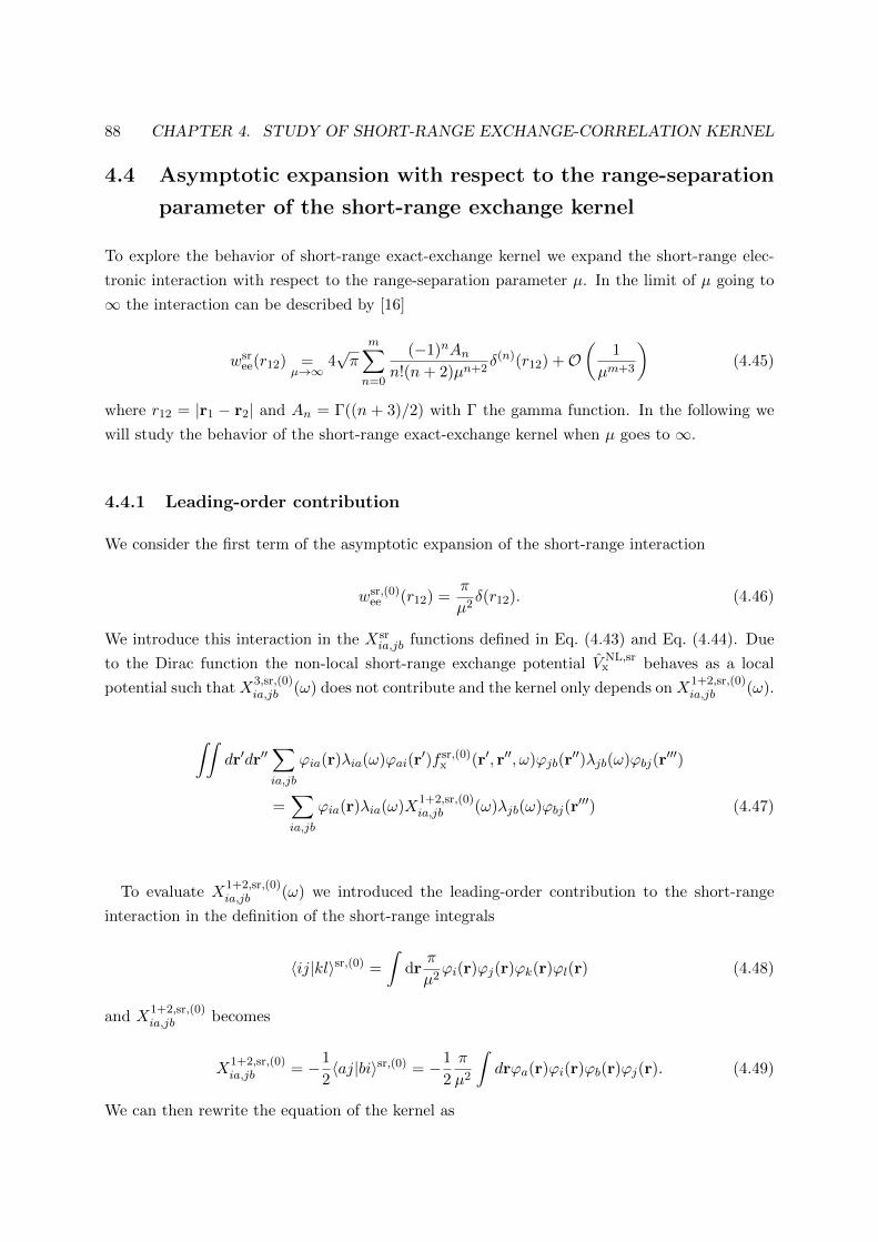
88 CHAPTER 4. STUDY OF SHORT-RANGE EXCHANGE-CORRELATION KERNEL
4.4 Asymptotic expansion with respect to the range-separation
parameter of the short-range exchange kernel
To explore the behavior of short-range exact-exchange kernel we expand the short-range elec-
tronic interaction with respect to the range-separation parameter µ. In the limit of µ going to
∞ the interaction can be described by [16]
wsree(r12) =
µ→∞4√π
m∑
n=0
(−1)nAnn!(n+ 2)µn+2
δ(n)(r12) +O(
1
µm+3
)(4.45)
where r12 = |r1 − r2| and An = Γ((n + 3)/2) with Γ the gamma function. In the following we
will study the behavior of the short-range exact-exchange kernel when µ goes to ∞.
4.4.1 Leading-order contribution
We consider the first term of the asymptotic expansion of the short-range interaction
wsr,(0)ee (r12) =
π
µ2δ(r12). (4.46)
We introduce this interaction in the Xsria,jb functions defined in Eq. (4.43) and Eq. (4.44). Due
to the Dirac function the non-local short-range exchange potential V NL,srx behaves as a local
potential such that X3,sr,(0)ia,jb (ω) does not contribute and the kernel only depends on X
1+2,sr,(0)ia,jb (ω).
∫∫dr′dr′′
∑
ia,jb
ϕia(r)λia(ω)ϕai(r′)f sr,(0)
x (r′, r′′, ω)ϕjb(r′′)λjb(ω)ϕbj(r
′′′)
=∑
ia,jb
ϕia(r)λia(ω)X1+2,sr,(0)ia,jb (ω)λjb(ω)ϕbj(r
′′′) (4.47)
To evaluate X1+2,sr,(0)ia,jb (ω) we introduced the leading-order contribution to the short-range
interaction in the definition of the short-range integrals
〈ij|kl〉sr,(0) =
∫dr
π
µ2ϕi(r)ϕj(r)ϕk(r)ϕl(r) (4.48)
and X1+2,sr,(0)ia,jb becomes
X1+2,sr,(0)ia,jb = −1
2〈aj|bi〉sr,(0) = −1
2
π
µ2
∫drϕa(r)ϕi(r)ϕb(r)ϕj(r). (4.49)
We can then rewrite the equation of the kernel as

4.4. ASYMPTOTIC EXPANSION OF THE SHORT-RANGE EXX KERNEL 89
∫∫dr′dr′′
∑
ia,jb
ϕia(r)λia(ω)ϕai(r′)f sr,(0)
x (r′, r′′, ω)ϕjb(r′′)λjb(ω)ϕbj(r
′′′)
=∑
ia,jb
ϕia(r)λia(ω)
[−1
2
π
µ2
∫d3r′ϕa(r′)ϕi(r′)ϕb(r
′)ϕj(r′)]λjb(ω)ϕjb(r
′′′), (4.50)
and by identification between the right-hand and the left-hand sides of the equation we can
determine the expression of the leading-order contribution to short-range exchange kernel
f sr,(0)x (r′, r′′, ω) = −1
2
π
µ2δ(r′ − r′′). (4.51)
4.4.2 Next-order contribution
We now consider the next-order contribution of the asymptotic expansion of the short-range
interaction
wsr,(1)ee (r12) = −4
3
√π
µ3δ(1)(r12) (4.52)
and introduce it in the expression of Xsria,jb. The next-order contribution vanishes because of the
integration over the angular degrees of freedom
∫dΩ1
∫dr12δ
(1)(r12)f(r12) = −∫
dΩ1u12 · ∇f |r12=0 = 0, (4.53)
where Ω1 stands for the angular coordinates associated to the variable r1. We can then express
the kernel as
f srx (r2, r3, ω) =
µ→∞−1
2
π
µ2δ(r2 − r3) +O
(1
µ4
)(4.54)
This result is consistent with results obtained from the study of the asymptotic expansion of the
exact ground-state short-range spin-independent exchange density functional for µ → ∞ [17]
and shows that the leading order term of the exact-exchange kernel is local in space and does
not depend on the frequency.
4.4.3 Examples of H2 and He
In this section we calculate the projection of the short-range exchange kernel in the molecular
orbital basis
(ia|f srx |jb) =
∫∫ϕi(r)ϕa(r)f sr
x (r, r′)ϕj(r′)ϕb(r′)drdr′ (4.55)
for two-electron systems in cc-pVDZ (abbreviated as VDZ) basis sets [18]. For two-electrons
systems the exact-exchange kernel can be related to the Hartree kernel as fEXXx = −1/2fH.

90 CHAPTER 4. STUDY OF SHORT-RANGE EXCHANGE-CORRELATION KERNEL
For two-electron systems, the EXX kernel is thus frequency independent. We will compare the
behavior of three kernels: the short-range LDA exchange kernel [17], the short-range exact-
exchange kernel and the short-range exact-exchange kernel when µ→∞ defined in Eq. (4.54).
The calculations were performed using the quantum chemistry program MOLPRO [19]. The
orbitals are calculated at the RSH level [20].
-0.2
-0.15
-0.1
-0.05
0
0 1 2 3 4 5
(ia|f
xsr |i
a)
µ
H2 / VDZ / R = eq/ RSH based
1σg → 1σu
fxsrEXX
fxsrLDA
fxsrEXX
(µ → ∞)-0.2
-0.15
-0.1
-0.05
0
0 1 2 3 4 5
(ia|f
xsr |i
a)
µ
H2 / VDZ / R = eq/ RSH based
1σg → 3πg
fxsrEXX
fxsrLDA
fxsrEXX
(µ → ∞)
-0.2
-0.15
-0.1
-0.05
0
0 1 2 3 4 5
(ia|f
xsr |i
a)
µ
H2 / VDZ / R = 10/ RSH based
1σg → 1σu
fxsrEXX
fxsrLDA
fxsrEXX
(µ → ∞) -0.2
-0.15
-0.1
-0.05
0
0 1 2 3 4 5
(ia|f
xsr |i
a)
µ
H2 / VDZ / R = 10/ RSH based
1σg → 3πg
fxsrEXX
fxsrLDA
fxsrEXX
(µ → ∞)
Figure 4.1: Projection of the short-range exchange kernel in the VDZ basis set (ia|f srx |ia) with
respect to the range-separation parameter µ for H2 at equilibrium (1.4 bohr) (top) and in thedissociation limit (distance of 10 bohr) (bottom) calculated with the short-range LDA, short-range exact-exchange and short-range exact exchange in the µ → ∞ limit. For each distancetwo transitions are shown: the first transition 1σg → 1σu and a higher transition 1σg → 3πg.
The results for H2 in VDZ are presented in Fig. 4.1. In this basis set we have one occupied
orbital and nine unoccupied orbitals, we only considered the diagonal terms of the kernel matrix.
In the limit of high µ we notice that the behavior of the three kernels are the same and that the
leading term of the expansion Eq. (4.54) gives a good description in this region. On the other
end of the curve, for µ→ 0 we can notice the difference of behavior between srLDA and srEXX:
srEXX seems to have a ”flatter” start than srLDA at µ→ 0. This difference of behavior could
be explained if we consider the behavior of both potentials (srLDA [17] and srEXX [21]) for
µ→ 0

4.4. ASYMPTOTIC EXPANSION OF THE SHORT-RANGE EXX KERNEL 91
-0.4
-0.3
-0.2
-0.1
0
0.1
0 1 2 3 4 5
(ia
|fxsr |i
a)
µ
He - VDZ
1s → 2s
srLDAsrEXX
srEXX (µ → ∞)-0.1
-0.08
-0.06
-0.04
-0.02
0
0 1 2 3 4 5
(ia
|fxsr |i
a)
µ
He - VDZ
1s → 2px, 2py, 2pz
srLDAsrEXX
srEXX (µ → ∞)
Figure 4.2: Projection of the short-range exchange kernel in VDZ basis set for He calculatedwith the short-range LDA, short-range exact-exchange and short-range exact exchange in theµ → ∞ limit. Two transitions are shown: the first transition 1s → 2s and a higher transition1s→ 2p.
vsr,EXXx (r) = vx(r) +
2µ√π
+ µ3vsr,(3)x (r) +O
(µ5)
(4.56)
vsr,LDAx (r) = vLDA
x (r) +µ√π− αµ2rs(r)
π+O
(e−1/µ2
), (4.57)
with rs = (3/(4πn))1/3 the Wigner-Seitz radius and α = (4/(9π))1/3. By taking the second-order
derivative of both potentials with respect to the density the corresponding kernels are
f sr,EXXx (r, r′) = fEXX
x (r, r′) + µ3 f sr,(3)x (r, r′) +O
(µ5)
(4.58)
f sr,LDAx (r, r′) = fLDA
x (r)δ(r− r′) + πα4r4s (r)µ2 +O
(e−1/µ2
), (4.59)
with fLDAx (r) = ∂2eLDA
x /∂n2 the second-order derivative of the LDA exchange energy density
with respect to the density. The srLDA exchange kernel in the limit of small µ should thus
be quadratic while the short-range EXX exchange kernel should behave as µ3. This seems
consistent with the behavior observed for H2 at equilibrium (however in the dissociation limit the
variation of the short-range EXX kernel seems to be faster for the first transition 1σg → 1σu).
It is interesting to remark that for localized valence excitation (1σg → 1σu at equilibrium)
srLDA gives good results with respect to srEXX even for µ close to 0. For Rydberg excitations
(1σg → 3πg at equilibrium and in the dissociation limit) and delocalized valence excitation
(1σg → 1σu in the dissociation limit) there is a loss of accuracy. We finally considered a second
system, the helium atom in the VDZ basis set, and the results are presented in Fig. 4.2. The
results for He are similar to H2: the local valence excitations are well described by srLDA.

92 CHAPTER 4. STUDY OF SHORT-RANGE EXCHANGE-CORRELATION KERNEL
4.5 Study of the exact frequency-dependent correlation kernel
In this section we want to extend our study of the short-range exchange kernel to the short-range
correlation kernel. The analytic derivation of the exact correlation kernel in a similar way to
Sec. 4.3 is complicated due to the definition of the correlation potential vc =∑∞
i=2−v(i). An
example of exploring the orbital-dependent correlation functionals with many-body perturbation
theory at second order is given by Bokhan and Bartlett [22]. A way to study the frequency
dependence is to consider the exact correlation kernel for a model system: H2 in minimal basis
set.
4.5.1 FCI of H2 in minimal basis set
The derivation of the short-range correlation kernel in this section will be based on a full-
configuration interaction (FCI) calculation in a minimal basis set. For H2 the minimal basis set
will be composed of two orthogonal orbitals ϕ1 and ϕ2 localized on the two hydrogen atoms.
The different determinants for H2 in this minimal basis set are presented in Fig. 4.3.
|11〉 |12〉 |12〉 |12〉 |12〉 |22〉
Figure 4.3: Determinants for H2 in a minimal basis set.
The wave-functions and energies obtained at the FCI level are obtained by solving the matrix
projection of the Hamiltonian on those determinants. The obtained results are
|0〉 = c1|11〉+ c2|22〉 E0 = 2ε1 − J11 + ∆−√
∆2 −K212
|1〉 = c′1|11〉+ c′2|22〉 E1 = 2ε1 − J11 + ∆ +√
∆2 −K212
|2〉 = 1√2
(|12〉+ |21〉) E3 = h11 + h22 + J12 +K12
|3〉 = |12〉 E3 = h11 + h22 + J12 −K12
|4〉 = |12〉 E4 = h11 + h22 + J12 −K12
|5〉 = 1√2
(|12〉 − |21〉) E5 = h11 + h22 + J12 −K12
(4.60)
with the coefficients for |0〉 defined by c21 + c2
2 = 1 and c2 = (∆ −√
∆2 +K212)/K12 and the
coefficients for |1〉 defined by (c′1)2 + (c′2)2 = 1 and c′2 = (∆ +√
∆2 +K212)/K12 with 2∆ =
2ε2−2ε1+J22−4J12+2K12+J11. The orbital energies are ε1 = h11+J11 and ε2 = h22+2J12−K12,

4.5. STUDY OF THE EXACT FREQUENCY-DEPENDENT CORRELATION KERNEL 93
hpp = 〈p|h|p〉 the one-electron integral and Jpq = 〈pq|pq〉 and Kpq = 〈pq|qp〉 the Coulomb and
exchange two-electrons integrals. The wave function |0〉 is the ground state, |1〉 and |2〉 are
singlet excited states and |3〉, |4〉 and |5〉 are triplet excited states. The integrals used to define
the different terms in the full-range Coulomb case can be taken from Ref. [23]. In the following
derivation of the short-range correlation kernel we will consider these states as starting point to
evaluate the linear-response function for both the full-range and long-range cases.
4.5.2 Calculation of the linear-response function
We want to calculate the exact linear-response function
χ(x1,x2; x′1,x′2;ω) =
∑
K 6=0
〈0|Ψ†(x′1)Ψ(x1)|K〉〈K|Ψ†(x′2)Ψ(x2)|0〉ω − (EK − E0) + i0+
(4.61)
−∑
K 6=0
〈0|Ψ†(x′2)Ψ(x2)|K〉〈K|Ψ†(x′1)Ψ(x1)|0〉ω + (EK − E0)− i0+
(4.62)
where Ψ(x) =∑iφi(x)ai, Ψ†(x) =
∑iφ∗i (x)a†i , |0〉 is the ground-state wave function and |K〉 are
the excited-states wave functions. It can be expressed in the basis of molecular orbitals
[χ(ω)]pq,rs =
∫dx1dx′1dx2dx′2φp(x
′1)φ∗q(x1)χ(x1,x2; x′1,x
′2;ω)φ∗r(x2)φs(x
′2) (4.63)
and using Eq. (4.61) it gives
[χ(ω)]pq,rs =∑
K 6=0
〈0|a†paq|K〉〈K|a†sar|0〉ω −∆EK + i0+
−∑
K 6=0
〈0|a†sar|K〉〈K|a†paq|0〉ω + ∆EK − i0+
(4.64)
with ∆EK = EK − E0. The linear-response function can be spin-adapted [24, 25, 26] into one
singlet block
1χpq,rs =1
2(χp↑q↑,r↑s↑ + χp↑q↑,r↓s↓ + χp↓q↓,r↑s↑ + χp↓q↓,r↓s↓) (4.65)
and three triplet blocks
3,0χpq,rs =1
2(χp↑q↑,r↑s↑ − χp↑q↑,r↓s↓ − χp↓q↓,r↑s↑ + χp↓q↓,r↓s↓) (4.66a)
3,1χpq,rs = −1
2(χp↑q↓,r↑s↓χp↑q↓,r↓s↑ + χp↓q↑,r↑s↓ + χp↓q↑,r↓s↑) (4.66b)
3,−1χpq,rs =1
2(χp↑q↓,r↑s↓ − χp↑q↓,r↓s↑ − χp↓q↑,r↑s↓ + χp↓q↑,r↓s↑) (4.66c)
where p, q, r and s refer now to spatial orbitals. We can express the singlet linear-response
function matrix as

94 CHAPTER 4. STUDY OF SHORT-RANGE EXCHANGE-CORRELATION KERNEL
[1χ(ω)
]pq,rs
=1
2
∑
K 6=0
〈0|Epq|K〉〈K|Esr|0〉ω −∆EK + i0+
−∑
K 6=0
〈0|Esr|K〉〈K|Epq|0〉ω + ∆EK − i0+
(4.67)
with Epq = a†p↑aq↑ + a†p↓aq↓. The triplet contributions 3,0χ,3,1χ and 3,−1χ can be obtained by
using√
2T 1,0 = a†p↑aq↑− a†p↓aq↓, T
1,1 = −a†p↑aq↓ and T 1,−1 = a†p↓aq↑, respectively, instead of Epq.
The matrix form of the singlet linear-response function is, in the occupied/virtual and vir-
tual/occupied block,
1χ(ω) =
c21
ω −∆E2 + i0+− c2
2
ω + ∆E2 − i0+
c1c2
ω −∆E2 + i0+− c1c2
ω + ∆E2 − i0+
c1c2
ω −∆E2 + i0+− c1c2
ω + ∆E2 − i0+
c22
ω −∆E2 + i0+− c2
1
ω + ∆E2 − i0+
. (4.68)
In the non-interacting limit (c1 → 1, c2 → 0), the Kohn-Sham response function, Eq. (4.13), is
obtained. The inverse singlet linear-response function is
1χ−1(ω) =
(ω −∆E2)c21 − (ω + ∆E2)c2
2
(c21 − c2
2)2
2∆E2c1c2
(c21 − c2
2)2
2∆E2c1c2
(c21 − c2
2)2
(ω −∆E2)c22 − (ω + ∆E2)c2
1
(c21 − c2
2)2
. (4.69)
Similarly, the matrix form of the triplet linear-response functions is
3,0χ(ω) =
c21
ω −∆E5 + i0+− c2
2
ω + ∆E5 − i0+− c1c2
ω −∆E5 + i0++
c1c2
ω + ∆E5 − i0+
− c1c2
ω −∆E5 + i0++
c1c2
ω + ∆E5 − i0+
c22
ω −∆E5 + i0+− c2
1
ω + ∆E5 − i0+
,
(4.70)
and the inverse is
3,0χ−1(ω) =
−c22(ω −∆E5) + c2
1(ω + ∆E5)
(c21 − c2
2)2
−2c1c2∆E5
(c21 − c2
2)2
−2c1c2∆E5
(c21 − c2
2)2
c22(ω −∆E5)− c2
1(ω + ∆E5)
(c21 − c2
2)2
. (4.71)
The χp↑q↓,r↓s↑ and χp↓q↑,r↑s↓ elements are equal to 0, 3,−1χ and 3,1χ are then equal and, as the
energies of the triplet states are degenerate, we can see that 3,0χ = 3,1χ = 3,−1χ.
4.5.3 Derivation of the exact short-range correlation kernel
The short-range kernel can be deduced from the difference of the inverse of the long-range
linear-response function and the inverse of the full-range linear-response function, as presented
in Eq. (4.16). The long-range linear-response function has the same expression as the full-range

4.5. STUDY OF THE EXACT FREQUENCY-DEPENDENT CORRELATION KERNEL 95
linear-response function calculated in Sec. 4.5.2 but evaluated with the long-range Hamiltonian
H = T + Wee + Vne → H lr = T + W lree + Vne + V sr
Hxc (4.72)
leading to the long-range orbital energies
ε1 → εlr1 = h11 + 2J11 −K lr11 + V sr
xc,11 (4.73a)
ε2 → εlr2 = h22 + 2J12 −K lr12 + V sr
xc,12 (4.73b)
with V srxc,ij =
∫drϕi(r)vsr
xc(r)ϕj(r) the integral of the short-range exchange-correlation potential
and the long-range Coulomb and exchange two-electrons integrals
Jpq → J lrpq = 〈pq|wlr
ee|pq〉 (4.74a)
Kpq → K lrpq = 〈pq|wlr
ee|qp〉. (4.74b)
The coefficients clr1 and clr
2 and the energy differences ∆ElrK have the same form as for the full-
range interaction but are evaluated using the long-range orbital energies and the long-range
two-electron integrals.
Introducing the linear-response function of Sec. 4.5.2 into Eq. (4.16) we obtain the singlet
and triplet Hartree-exchange-correlation kernels
1f srHxc(ω) =
∆E2
(c21−c22)2− ∆Elr
2
((clr1 )2−(clr2 )2)2−2c1c2∆E2
(c21−c22)2+
2clr1 clr2 ∆Elr
2
((clr1 )2−(clr2 )2)2
−2c1c2∆E2
(c21−c22)2+
2clr1 clr2 ∆Elr
2
((clr1 )2−(clr2 )2)2∆E2
(c21−c22)2− ∆Elr
2
((clr1 )2−(clr2 )2)2
+ ω
−
1(c21−c22)2
+ 1((clr1 )2−(clr2 )2)2
0
0 1(c21−c22)2
− 1((clr1 )2−(clr2 )2)2
, (4.75)
3f srHxc(ω) =
∆E5
(c21−c22)2− ∆Elr
5
(clr12)2−2c1c2∆E5
(c21−c22)2+
2clr1 clr2 ∆Elr
5
((clr1 )2−(clr2 )2)2
−2c1c2∆E5
(c21−c22)2+
2clr1 clr2 ∆Elr
5
(clr12)2∆E5
(c21−c22)2− ∆Elr
5
((clr1 )2−(clr2 )2)2
+ ω
−
1(c21−c22)2
+ 1((clr1 )2−(clr2 )2)2
0
0 1(c21−c22)2
− 1((clr1 )2−(clr2 )2)2
. (4.76)
The singlet and triplet short-range Hartree kernels are
1f srH =
(2K12 − 2K lr
12 2K12 − 2K lr12
2K12 − 2K lr12 2K12 − 2K lr
12
)=
(2Ksr
12 2Ksr12
2Ksr12 2Ksr
12
), (4.77)

96 CHAPTER 4. STUDY OF SHORT-RANGE EXCHANGE-CORRELATION KERNEL
3f srH =
(0 0
0 0
). (4.78)
The singlet short-range exchange-correlation kernel is then
1f srxc(ω) =
∆E2
(c21−c22)2− ∆Elr
2
((clr1 )2−(clr2 )2)2− 2Ksr
12 −2c1c2∆E2
(c21−c22)2+
2clr1 clr2 ∆Elr
2
((clr1 )2−(clr2 )2)2− 2Ksr
12
−2c1c2∆E2
(c21−c22)2+
2clr1 clr2 ∆Elr
2
((clr1 )2−(clr2 )2)2− 2Ksr
12∆E2
(c21−c22)2− ∆Elr
2
((clr1 )2−(clr2 )2)2− 2Ksr
12
+ ω
−
1(c21−c22)2
+ 1((clr1 )2−(clr2 )2)2
0
0 1(c21−c22)2
− 1((clr1 )2−(clr2 )2)2
(4.79)
and the triplet short-range exchange-correlation kernel is
3f srxc(ω) =
∆E5
(c21−c22)2− ∆Elr
5
(clr12)2−2c1c2∆E5
(c21−c22)2+
2clr1 clr2 ∆Elr
5
((clr1 )2−(clr2 )2)2
−2c1c2∆E5
(c21−c22)2+
2clr1 clr2 ∆Elr
5
(clr12)2∆E5
(c21−c22)2− ∆Elr
5
((clr1 )2−(clr2 )2)2
+ ω
−
1(c21−c22)2
+ 1((clr1 )2−(clr2 )2)2
0
0 1(c21−c22)2
− 1((clr1 )2−(clr2 )2)2
. (4.80)
We will consider two ways of calculating the short-range exchange kernel. We will first consider
the HF exchange kernel
1f sr,HFx = 3f sr,HF
x =
(−J12 + J lr
12 −K12 +K lr12
−K12 +K lr12 −J12 + J lr
12
)=
(−J sr
12 −Ksr12
−Ksr12 −J sr
12
), (4.81)
and the (spin-independent) exact-exchange presented in Sec. 4.3
1f sr,EXXx = −1
21f sr
H =
(−K12 +K lr
12 −K12 +K lr12
−K12 +K lr12 −K12 +K lr
12
)=
(−Ksr
12 −Ksr12
−Ksr12 −Ksr
12
), (4.82)
3f sr,EXXx = −1
23f sr
H =
(0 0
0 0
). (4.83)
If the exchange contribution is the short-range Hartree-Fock exchange kernel the singlet and
triplet short-range correlation kernels are

4.5. STUDY OF THE EXACT FREQUENCY-DEPENDENT CORRELATION KERNEL 97
1f sr, postHFc (ω) =
∆E2
(c21−c22)2− ∆Elr
2
((clr1 )2−(clr2 )2)2− 2Ksr
12 + J sr12 −2c1c2∆E2
(c21−c22)2+
2clr1 clr2 ∆Elr
2
((clr1 )2−(clr2 )2)2−Ksr
12
−2c1c2∆E2
(c21−c22)2+
2clr1 clr2 ∆Elr
2
((clr1 )2−(clr2 )2)2−Ksr
12∆E2
(c21−c22)2− ∆Elr
2
((clr1 )2−(clr2 )2)2− 2Ksr
12 + J sr12
+ ω
−
1(c21−c22)2
+ 1((clr1 )2−(clr2 )2)2
0
0 1(c21−c22)2
− 1((clr1 )2−(clr2 )2)2
, (4.84)
3f sr, postHFc (ω) =
∆E5
(c21−c22)2− ∆Elr
5
(clr12)2+ J sr
12 −2c1c2∆E5
(c21−c22)2+
2clr1 clr2 ∆Elr
5
((clr1 )2−(clr2 )2)2+Ksr
12
−2c1c2∆E5
(c21−c22)2+
2clr1 clr2 ∆Elr
5
(clr12)2+Ksr
12∆E5
(c21−c22)2− ∆Elr
5
((clr1 )2−(clr2 )2)2+ J sr
12
+ ω
−
1(c21−c22)2
+ 1((clr1 )2−(clr2 )2)2
0
0 1(c21−c22)2
− 1((clr1 )2−(clr2 )2)2
. (4.85)
On the other hand, if the exchange contribution is the short-range exact-exchange kernel the
singlet and triplet short-range correlation kernels are
1f sr, postEXXc (ω) =
∆E2
(c21−c22)2− ∆Elr
2
((clr1 )2−(clr2 )2)2−Ksr
12 −2c1c2∆E2
(c21−c22)2+
2clr1 clr2 ∆Elr
2
((clr1 )2−(clr2 )2)2−Ksr
12
−2c1c2∆E2
(c21−c22)2+
2clr1 clr2 ∆Elr
2
((clr1 )2−(clr2 )2)2−Ksr
12∆E2
(c21−c22)2− ∆Elr
2
((clr1 )2−(clr2 )2)2−Ksr
12
+ ω
−
1(c21−c22)2
+ 1((clr1 )2−(clr2 )2)2
0
0 1(c21−c22)2
− 1((clr1 )2−(clr2 )2)2
, (4.86)
3f sr, postEXXc (ω) =
∆E5
(c21−c22)2− ∆Elr
5
(clr12)2−2c1c2∆E5
(c21−c22)2+
2clr1 clr2 ∆Elr
5
((clr1 )2−(clr2 )2)2
−2c1c2∆E5
(c21−c22)2+
2clr1 clr2 ∆Elr
5
(clr12)2∆E5
(c21−c22)2− ∆Elr
5
((clr1 )2−(clr2 )2)2
+ ω
−
1(c21−c22)2
+ 1((clr1 )2−(clr2 )2)2
0
0 1(c21−c22)2
− 1((clr1 )2−(clr2 )2)2
. (4.87)
In all cases if we compare both kernels we can see that the frequency dependence is the same
for the singlet and the triplet kernels.

98 CHAPTER 4. STUDY OF SHORT-RANGE EXCHANGE-CORRELATION KERNEL
-0.6
-0.5
-0.4
-0.3
-0.2
-0.1
0
0.1
0 1 2 3 4 5 6 7 8 9 10
f c (
hart
ree)
µ (bohr-1
)
[fc (ω = 0) ]12,12 postEXX
[fc (ω = 0)]12,12 postHF
[fc (ω = 0)]12,21
[∆ fc (ω = 1) ]12,12 0.1
0.15
0.2
0.25
0.3
0.35
0.4
0.45
0.5
0.55
0.6
0 1 2 3 4 5
∆ f
c (
ω=
1)/
fc (
ω =
0)
µ (bohr-1
)
postEXX
postHF
-1e+07
-9e+06
-8e+06
-7e+06
-6e+06
-5e+06
-4e+06
-3e+06
-2e+06
-1e+06
0
0 1 2 3 4 5 6 7 8 9 10
f c (
hart
ree)
µ (bohr-1
)
[fc (ω = 0) ]12,12 postEXX
[fc (ω = 0)]12,12 postHF
[fc (ω = 0)]12,21
[∆ fc (ω = 1) ]12,12 0.9
1
1.1
1.2
1.3
1.4
1.5
0 1 2 3 4 5
∆ f
c (
ω=
1)/
fc (
ω =
0)
µ (bohr-1
)
postEXX
postHF
Figure 4.4: Contributions to the singlet short-range correlation kernel for H2 in STO-3G. Weplotted the diagonal element of the frequency-dependent matrix [∆1fc(ω = 1)]12,12, the diagonalelements of the frequency-independent matrix [1fc(ω = 0)]12,12 and the off-diagonal elementsof the frequency-independent matrix [1fc(ω = 0)]12,21 with respect to µ (left) and the ratio|∆1fc(ω)/1fc(ω = 0)| for both HF and EXX exchange with respect to µ (right). These resultsare calculated at equilibrium distance (1.4 bohr) (top) and when stretching the H-H bond (10bohr) (bottom). On the bottom plot the curves for the 1f sr
c (ω = 0) are superimposed.
4.5.4 Calculations on H2 in STO-3G basis
We calculate the different terms of the singlet short-range correlation kernel [Eqs. (4.84) and
(4.86)] by performing calculations using the MOLPRO software [19] with the STO-3G basis set.
The long-range coefficients and energies are calculated with FCI with long-range Hamiltonian
using a fixed RSH density [20] and full-range coefficients and energies are calculated with FCI
with the full-range Hamiltonian. The Coulomb and exchange integrals J12 and K12 are extracted
from the TDDFT module. We decompose the kernel matrix in two matrices: the frequency-
independent term 1fc(ω = 0) and the frequency-dependent term common to both singlet and
triplet kernel ∆1fc(ω) = 1fc(ω) − 1fc(ω = 0). In the calculations the frequency-dependent
kernel is evaluated at ω = 1 (hartree) as representative of the order of magnitude of electronic
excitations in atoms and molecules. The results are presented in Fig. 4.4. We first consider the
evolution of the kernel elements with respect to the range-separation parameter µ and we can

4.5. STUDY OF THE EXACT FREQUENCY-DEPENDENT CORRELATION KERNEL 99
-2
-1.5
-1
-0.5
0
0.5
0 1 2 3 4 5 6 7 8 9 10
f c ×
µ2 (
hart
ree)
µ (bohr-1
)
[fc (ω = 0) ]12,12 postEXX
[fc (ω = 0)]12,12 postHF
[fc (ω = 0)]12,21
[∆ fc (ω = 1) ]12,12-7e+06
-6e+06
-5e+06
-4e+06
-3e+06
-2e+06
-1e+06
0
0 1 2 3 4 5 6 7 8 9 10
f c ×
µ2 (
hart
ree)
µ (bohr-1
)
[fc (ω = 0) ]12,12 postEXX
[fc (ω = 0)]12,12 postHF
[fc (ω = 0)]12,21
[∆ fc (ω=1) ]12,12
Figure 4.5: Product of fc×µ2 with respect to µ at equilibrium distance (1.4 bohr) (left) and afterstretching the H-H bond (10 bohr) (right) for H2 in STO-3G. We considered the diagonal elementof the frequency-dependent matrix [∆1fc(ω = 1)]12,12, the diagonal elements of the frequency-independent matrix [1fc(ω = 0)]12,12 and the off diagonal elements of the frequency-independentmatrix [1fc(ω = 0)]12,21.
-20
-15
-10
-5
0
0 1 2 3 4 5 6 7 8
f c (
hart
ree)
R (bohr)
[fc (ω = 0) ]12,12 postEXX
[fc (ω = 0)]12,12 postHF
[fc (ω = 0)]12,21
[∆ fc (ω=1) ]12,12
Figure 4.6: Contributions to the singlet kernel for H2 in STO-3G. We plotted the diagonalelement of the frequency-dependent matrix [∆1fc(ω = 1)]12,12, the diagonal elements of thefrequency-independent matrix [1fc(ω = 0)]12,12 and the off diagonal elements of the frequency-independent matrix[1fc(ω = 0)]12,21 with respect to R at µ = 0.4

100 CHAPTER 4. STUDY OF SHORT-RANGE EXCHANGE-CORRELATION KERNEL
notice that the amplitude of the frequency-dependent term is small compared to the elements
of the frequency-independent matrix. We considered the ratio of |∆1fc(ω = 1)/1fc(ω = 0)| and
we can notice that for µ ≥ 0.9 bohr−1 for postHF and µ ≥ 1.8 bohr−1 for postEXX the ratio
is constant showing the similar asymptotic behavior of the frequency-dependent and frequency-
independent contributions of the singlet kernel. The ratio converges to 0.18 this value is small
and the adiabatic approximation is thus good for the short range correlation kernel but it remains
an approximation. We plotted in Fig. 4.5 the product fc × µ2. The fact that the curves go
to some constants for µ → ∞ indicates that the asymptotic behavior of the contributions to
the correlation kernel behaves as 1/µ2. We then considered the evolution of the kernel elements
with respect to the internuclear distance R at µ = 0.4 bohr−1 which is an optimal value in
range-separated TDDFT. The result is presented in Fig. 4.6. We notice that all the terms have
a similar behavior and diverge for large R. We studied the behavior of the correlation term while
stretching the H-H bond (at R = 10 bohr) we first notice that there is no longer a difference
between postHF and postEXX terms, the leading term of the kernel is given by the difference
of the coefficients c1 and c2 (and clr1 and clr
2 ) that are nearly degenerate and make the terms
diverge. Thus the amplitude of the kernel is more important than for the equilibrium. The ratio
|∆1fc(ω = 1)/1fc(ω = 0)| converges slower and to a higher value than at equilibrium (' 1) which
implies that in this case the frequency-dependent term is more important and that the adiabatic
approximation is less accurate. Finally we can see in Fig. 4.5 that the asymptotic behavior
of the frequency-dependent and frequency-independent terms remain as 1/µ2. To extend this
work it would be interesting to study the effect of this exact short-range correlation kernel on
the bond-breaking 1Σg −1 Σu excitation energy to see if it could compensate the decay to zero
of the excitation energy observed for the adiabatic approximation.
4.6 Conclusion
In this work, we have studied the short-range exchange and correlation kernels. We first extended
the EXX time-dependent density-functional theory to range separation and studied the asymp-
totic expansion of the short-range EXX kernel as a function of the range-separation parameter.
We showed that the two first terms of this asymptotic expansion are frequency-independent
and local in space. We then compared the performance of this short-range EXX kernel to the
short-range LDA kernel for two simple systems: H2 and He in the VDZ basis set. We showed
that in the limit of large µ the semilocal approximation becomes exact but when µ goes to 0 the
semilocal approximation has limitations with a good behavior for localized valence excitation
energies but less accurate results for Rydberg and delocalized valence excitation energies.
In the second part of this chapter we studied the short-range correlation kernel by studying
the exact short-range correlation kernel for a model system: H2 in a minimal basis set. We
first derived the short-range correlation kernel and noticed that for this system the frequency
dependence is the same for both singlet and triplet kernels and that it does not depend on the

4.6. CONCLUSION 101
nature of the exchange contribution (HF or EXX). We continued this study with practical calcu-
lations for H2 in the STO-3G basis and we showed that even in the limit of large µ the adiabatic
approximation is not exact. This frequency dependent term is relatively small at equilibrium
but becomes large in the dissociation limit.
In further work the study of the short-range exchange kernel could be extended by deriving the
next term of the asymptotic expansion. This term would be in 1/µ4 and should be frequency
dependent. An implementation work could be also done to describe larger systems and study the
adiabatic semilocal approximation in more complicated examples implying double excitations.

102 BIBLIOGRAPHY
Bibliography
[1] E. Runge and E. K. U. Gross. Density-Functional Theory for Time-Dependent Systems.
Phys. Rev. Lett. , 52:997, 1984.
[2] M. Thiele and S. Kummel. Frequency Dependence of the Exact Exchange-Correlation
Kernel of Time-Dependent Density-Functional Theory. Phys. Rev. Lett. , 112:083001, 2014.
[3] A. Dreuw, J. L. Weisman, and M. Head-Gordon. Long-range charge-transfer excited states
in time-dependent density functional theory require non-local exchange. J. Chem. Phys. ,
119:2943, 2003.
[4] A. Heßelmann, A. Ipatov, and A. Gorling. Charge-transfer excitation energies with a time-
dependent density-functional method suitable for orbital-dependent exchange-correlation
kernels. Phys. Rev. A, 80:012507, 2009.
[5] S. Hirata and M. Haed-Gordon. Time-dependent density functional theory for radicals:
An improved description of excited states with substantial double excitation character.
Chem. Phys. Lett. , 302:375, 1999.
[6] N. T. Maitra, F. Zhang, R. J. Cave, and K. Burke. Double excitations within time-
dependent density functional theory linear response. J. Chem. Phys. , 120:5932, 2004.
[7] K. J. H. Giesbertz and E. J. Baerends. Failure of time-dependent density functional theory
for excited state surfaces in case of homolytic bond dissociation. Chem. Phys. Lett. , 461:338,
2008.
[8] A. Savin. On Degeneracy, Near Degeneracy and Density Functional Theory. In J. M.
Seminario, editor, Recent Developments of Modern Density Functional Theory, pages 327–
357. Elsevier, Amsterdam, 1996.
[9] Y. Tawada, T. Tsuneda, S. Yanagisawa, and K. Hirao. A long-range-corrected time-
dependent density functional theory. J. Chem. Phys. , 120:8425, 2004.
[10] K. Pernal. Excitation energies form range-separated time-dependent density and density
matrix functional theory. J. Chem. Phys. , 136:184105, 2012.
[11] E. Fromager, S. Knecht, and H. J. A. Jensen. Multi-configuration time-dependent density-
functional theory based on range separation. J. Chem. Phys. , 138:084101, 2013.
[12] A. Gorling. Time-dependent Kohn-Sham formalism. Phys. Rev. A, 55:2630, 1997.
[13] A. Gorling. Exact exchange-correlation kernel for dynamic response porperties and excita-
tion energies in density-functional theory. Phys. Rev. A, 57:3433, 1998.

BIBLIOGRAPHY 103
[14] A. Gorling. Exact-Exchange Methods and Perturbation Theory along the Adiabatic Con-
nection. In Miguel A.L. Marques, Carsten A. Ullrich, Fernando Nogueira, Angel Rubio,
Kieron Burke, and Eberhard U. K. Gross, editors, Time-Dependent Density Functional
Theory, pages 137–159. Springer Berlin Heidelberg, Berlin, Heidelberg, 2006.
[15] A. Ipatov, A. Heßelmann, and A. Gorling. Molecular Excitation Spectra by TDDFT With
the Nonadiabatic Exact Exchange Kernel. Int. J. Quantum Chem. , 110:2202, 2010.
[16] J. Toulouse, F. Colonna, and A. Savin. Long-range–short-range separation of the electron-
electron interaction in density-functional theory. PRA, 70(6):062505, 2004.
[17] E. Rebolini, A. Savin, and J. Toulouse. Electronic excitations from a linear-response range-
separated hybrid scheme. Mol. Phys. , 111:1219, 2013.
[18] T. H. Dunning. Gaussian basis sets for use in correlated molecular calculations. I. The
atoms boron through neon and hydrogen. J. Chem. Phys., 90:1007, 1989.
[19] H.-J. Werner, P. J. Knowles, G. Knizia, F. R. Manby, M. Schutz, and others. MOLPRO,
version 2015.1, a package of ab initio programs. Cardiff, UK, 2015, see http://www.molpro.
net.
[20] J. G. Angyan, I. C. Gerber, A. Savin, and J. Toulouse. Van der Waals forces in density
functional theory: Perturbational long-range electron-interaction corrections. Phys. Rev. A,
72:012510, 2005.
[21] E. Rebolini, J. Toulouse, A. M. Teale, T. Helgaker, and A. Savin. Excitation energies along
a range-separated adiabatic connection. J. Chem. Phys. , 141:044123, 2014.
[22] D. Bokhan and R. J. Bartlett. Adiabatic ab initio time-dependent density-functional
theory employing optimized-effective-potential many-body perturbation theory potentials.
Phys. Rev. A, 73:022502, 2006.
[23] M. J. S. Dewar and J. Kelemen. LCAO MO Theory Illustrated by Its Application to H2.
J. Chem. Edu., 48:495, 1971.
[24] J. Toulouse, W. Zhu, A. Savin, G. Jansen, and J. G. Angyan. Closed-shell ring coupled
cluster doubles theory with range separation applied on weak intermolecular interactions.
J. Chem. Phys. , 135:084119, 2011.
[25] J. G. Angyan, R.-F. Liu, J. Toulouse, and G. Jansen. Correlation energy expressions from
the adiabatic-connection fluctuation-dissipation theorem approach. J. Chem. Theory Com-
put., 7:3116, 2011.
[26] E. Rebolini, J. Toulouse, and A. Savin. Electronic excitation energies of molecular systems
from the Bethe-Salpeter equation: Example of the H2 molecule. In S. K. Ghosh and P. K.

104 BIBLIOGRAPHY
Chattaraj, editors, Electronic Structure and Reactivity, Concepts and Methods in Modern
Theoretical Chemistry Vol. 1, pages 367–390. CRC Press, 2013.

Conclusion
In this thesis we were interested in the study of hybrid approximations between wave-function
based methods and density-functional theory considering two ways of decomposing the electron-
electron interaction: linearly or with range separation. We performed three separate studies.
The first chapter presented in this work was focused on the basis-set convergence in the
range-separated scheme. We performed two studies to compare and characterize the basis-set
convergence in full-range and range-separated methods. We have first shown that the partial-
wave expansion of the long-range wave function near the electron-electron coalescence converges
exponentially with the maximal angular momentum L. We then have shown that the long-range
correlation energy error evaluated with the second-order Møller-Plesset perturbation theory was
converging exponentially with respect to the cardinal number of the Dunning basis sets cc-
pVXZ. This is an acceleration with respect to the full-range case where the convergence is
polynomial (X3). While studying the basis-set convergence we noticed that the Dunning basis
sets may not be optimal to perform calculations with range-separated methods. The results
obtained in this chapter are expected to be similar when using other methods to describe the
long-range correlation such as configuration interaction, coupled-cluster theory or random-phase
approximations.
The second chapter was focused on double-hybrid methods and particularly on a self-consistent
way to include the MP2 correlation energy using an optimized-effective-potential (OEP) method.
The aim of this study was to compare the performance of such self-consistent double-hybrid
approximation to the standard double-hybrid approximation. A one-parameter self-consistent
double-hybrid approximation has first been implemented. We considered a set of atoms and
molecules and compared some properties such as ionization potentials and electronic affinities.
We observed no improvement for total energies and ionization potentials but we obtained good
estimates for LUMO orbital energies and good accuracy for electronic affinities. An interesting
result is that this self-consistent approximation give reasonably good accuracy for the exchange-
correlation and correlation potentials and correlated densities.
In the last chapter we considered range-separated linear-response time-dependent density-
functional theory and we studied the short-range exchange and correlation kernels. After ex-
105

106 CONCLUSION
tending the exact-exchange TDDFT to range-separation we proposed an asymptotic expansion
of the short-range exact-exchange kernel with respect to the range-separation parameter µ. The
first terms of the asymptotic expansion of the short-range exact-exchange kernel are both adia-
batic and local in space. The practical calculations performed for He and H2 in the VDZ basis
set showed an exact behavior for short-range LDA in the limit of large µ. We extended our
work on the short-range exact correlation kernel for H2 in a minimal basis set. Calculations in
STO-3G basis set showed that even for the short-range correlation kernel at large value of µ the
adiabatic approximation is not exact. The error coming from adiabatic approximation is even
more important in the dissociation limit of H2.
These studies can be extended and the perspectives are the following:
• A first point which could be of interest would be to define basis sets that would be optimal
for performing range-separated calculations.
• To extend the study on the OEP-based double-hybrid approximation a first step would
be to consider a comparison based on a larger set of systems and including other orbital-
optimized double-hybrid approximations such as the one proposed by Peverati and Head-
Gordon. A second step would be to extend this self-consistent double-hybrid approxima-
tion to range-separation or to the calculation of excited states by applying linear-response
time-dependent density-functional theory on this self-consistent double-hybrid approxima-
tion.
• The short-range exchange kernel could be extended by deriving the next term of the
asymptotic expansion. This term would be in 1/µ4 and should be frequency dependent.
An implementation work could be done also to describe greater systems and study the adi-
abatic semilocal approximation in more complicated examples implying double excitations
for both short-range exchange and correlation kernels.

Appendix A
Additional results for the basis-set
convergence of the long-range
correlation energy
In this appendix, complementary results to the study in Chapter 2 are presented.
A.1 Convergence of the correlation energy including core
electrons
The results presented in the article are given for valence-only calculations. We extended
the study to calculations including the core excitations. The long-range MP2 correlation
energies including core excitations and the errors with respect to the energy calculated
in cc-pCV6Z are presented in Tab. A.1. In this case the approximation of taking the
calculations at X = 6 as a converged reference is still valid. We then compared the fits
for the polynomial law Elr,µc,X = Elr,µ
c,∞ + AX−α and the exponential law Elr,µc,X = Elr,µ
c,∞ +
B exp(−βX). The results of the fits for the long-range MP2 correlation energy including
core excitations are presented in Tab. A.2. There is an important difference between the
results of the two fits. Similarly to the results for valence-only calculations the best fit is
obtained for the exponential law by far with r2 > 99%.
107

108 APPENDIX B. ADDITIONAL RESULTS ON BASIS-SET CONVERGENCE
Table A.1: MP2 correlation energies and their errors (in mhartree) for the long-range interactionat µ = 0.5 bohr−1 (Elr
c and ∆Elrc ) calculated with core Dunning basis sets of increasing sizes for
Ne, N2 and H2O. The errors are calculated with respect to the cc-pCV6Z values.
Long-range interactionµ = 0.5
Ne N2 H2OBasis set Elr
c ∆Elrc Elr
c ∆Elrc Elr
c ∆Elrc
cc-pCVDZ -0.7003 1.9640 -20.3491 3.2790 -6.4989 3.5277cc-pCVTZ -1.7941 0.8702 -22.8333 0.7949 -8.9992 1.0274cc-pCVQZ -2.3358 0.3285 -23.4009 0.2272 -9.6617 0.3649cc-pCV5Z -2.5675 0.0967 -23.5651 0.0631 -9.9344 0.0922cc-pCV6Z -2.6642 -23.6282 -10.0266
Table A.2: Results of the fits to the power and exponential laws of the long-range MP2 correlationenergy error ∆Elr
c,X for µ = 0.5 bohr−1. Different ranges Xmin ≤ X ≤ Xmax, for the cardinalnumber X of the core Dunning basis sets are tested. The parameters A and B are in mhartree.The squared Pearson correlation coefficients r2 of the fits are indicated in %.
Long-range interactionPower law Exponential law
Xmin Xmax α A r2 β B r2
Ne 2 5 -3.1969 22.1531 95.04 -1.0007 16.0226 99.173 5 -4.2572 100.9000 98.11 -1.0984 24.4685 99.58
N2 2 5 -4.2522 71.3488 98.79 -1.3105 43.1576 99.923 5 -4.9313 188.4132 99.37 -1.2668 35.7243 100.00
H2O 2 5 -3.8597 59.9484 97.39 -1.1968 38.9700 99.733 5 -4.6663 189.9653 97.64 -1.2053 40.4372 99.34
A.2 Extrapolation scheme
In Chapter 2, based on the exponential convergence of both the RSH and long-range MP2
energies we proposed an extrapolation formula for the total energy in the complete-basis-
set (BSE) limit based on three calculations in three successive basis sets of cardinal number
X, Y and Z (Y = X + 1 and Z = Y + 1) given by
E∞ = EXY Z =E2Y − EXEZ
2EY − EX − EZ. (A.1)
In this section we compare two ways to apply the extrapolation scheme. The first one, pre-
sented in the chapter 2 is simply to apply the formula of Eq. (A.1) to the total RSH+lrMP2
energy
EtotalXY Z = ERSH+lrMP2
XY Z , (A.2)

A.2.0 Extrapolation scheme 109
and the second way to do this extrapolation is to extrapolate separately the RSH and the
long-range MP2 correlation energies
EtotalXY Z = ERSH
XY Z + ElrMP2c,XY Z . (A.3)
We compared these two ways of performing the three-point extrapolation. The results for
the long-range MP2 correlation energy calculated with only valence excitations are given in
Tab. A.3 and the results for the long-range MP2 correlation energy including excitations
from the core orbitals are presented in Tab. A.4. In each case we were interested to
compare the error of the extrapolation to the error of the energy evaluated at different
X. For the energy with only valence excitations (Tab. A.3) the results for the separated
and the global extrapolation are similar (or even equal). For the calculations including
the core excitations (Tab. A.4) we first consider the results for the global extrapolation.
In this case we obtain results that have negative errors and generally, in a similar way
to the valence-only calculations, the separated extrapolation shows an improvement with
respect to the calculation at X = 4. If we compare the global and separated way to do
the three-point extrapolations for the calculations with the core excitations we can see
that the results are close. We can conclude that there is no notable difference between
those two extrapolations at a chemical accuracy level and that the global extrapolation is
sufficient.

110 APPENDIX B. ADDITIONAL RESULTS ON BASIS-SET CONVERGENCE
Table A.3: Errors (in mhartree) on the total RSH+lrMP2 energy, E = ERSH + Elr,MP2c , ob-
tained with cc-pVXZ basis sets form X = 2 to X = 5 (∆EX = EX − E6) and the errorsobtained with the three point extrapolation formula of Eq. (A.1) using X = 2, Y = 3, Z = 4(∆EDTQ = EDTQ − E6 evaluated for the total energy (ERSH+lrMP2) or evaluated for RSH andlrMP2 separately and recombined a posteriori (ERSH +ElrMP2
c ). The errors are calculated withrespect to the cc-pV6Z total energy for several values of the range-separation parameter µ (inbohr−1). Only valence excitations are included in the MP2 calculations.
µ ∆EµD ∆EµT ∆EµQ ∆Eµ5 ∆EµDTQ ∆EµDTQ
ERSH+lrMP2 ERSH + ElrMP2c
He 0.1 8.508 0.772 0.261 0.089 0.224 0.2240.5 8.488 0.781 0.245 0.078 0.205 0.1611.0 8.258 0.924 0.259 0.078 0.192 0.144
Ne 0.1 72.999 20.215 5.842 0.716 0.464 0.4620.5 74.523 20.337 5.763 0.751 0.401 0.1631.0 79.311 20.962 5.726 0.803 0.342 0.342
N2 0.1 47.061 13.026 4.136 0.853 0.993 0.9920.5 51.581 13.406 4.090 0.810 1.083 1.0831.0 61.053 15.108 4.513 0.868 1.337 1.303
H2O 0.1 54.861 15.229 5.005 0.857 1.451 1.4510.5 55.850 14.736 4.499 0.726 1.105 1.1021.0 61.013 15.212 4.423 0.724 1.099 1.087
Table A.4: Errors (in mhartree) on the total RSH+lrMP2 energy, E = ERSH +ElrMP2c , obtained
with cc-pVXZ basis sets form X = 2 to X = 5 (∆EX = EX − E6) and the errors obtainedwith the three point extrapolation formula of Eq. (A.1) using X = 2, Y = 3, Z = 4 (∆EDTQ =EDTQ − E6) evaluated for the total energy (ERSH+lrMP2) or evaluated for RSH and lrMP2separately and recombined a posteriori (ERSH +ElrMP2
c ). The errors are calculated with respectto the cc-pV6Z total energy for several values of the range-separation parameter µ (in bohr−1).Core and valence excitations are included in the MP2 calculations.
µ ∆EµD ∆EµT ∆EµQ ∆Eµ5 ∆EµDTQ ∆EµDTQ
ERSH+lrMP2 ERSH + ElrMP2c
Ne 0.1 79.932 18.941 4.929 0.522 -0.240 -0.2410.5 72.501 18.990 4.831 0.537 -0.263 -0.4791.0 77.497 19.517 4.775 0.554 -0.250 -0.250
N2 0.1 43.528 10.237 2.334 0.459 -0.126 -0.1270.5 48.079 10.451 2.285 0.413 0.021 0.0201.0 57.942 12.118 2.677 0.467 0.227 0.222
H2O 0.1 52.875 13.897 4.132 0.680 0.868 0.8670.5 53.936 13.789 3.527 0.521 0.539 0.536

Appendix B
Derivation of the exact-exchange
kernel
In this appendix, we present a detailed derivation of the exact-exchange (EXX) kernel
[1]. This has to be read together with Chapter 4.
To express the EXX kernel we need to take the functional derivative with respect
to the time-dependent Kohn-Sham (KS) potential vKS(r, t) of the time-dependent EXX
(TDEXX) equation
∫ t
t0
dt′∫
dr′χ0(r, t; r′, t′)vx(r′, t′) = Λx(r, t) (B.1)
with the Kohn-Sham linear-response function (for closed shell systems)
χ0(r, t; r′, t′) = 2(−i)occ.∑
i
unocc.∑
a
ϕ∗i (r, t)ϕa(r, t)ϕ∗a(r′, t′)ϕi(r′, t′) + c.c. (B.2)
and the right-hand-side term
Λx(r, t) =2(−i)occ.∑
i
unocc.∑
a
ϕ∗i (r, t)ϕa(r, t)∫ t
t0
dt′〈ϕa(t′)|V NLx (t′)|ϕi(t′)〉+ c.c. (B.3)
+ 2occ.∑
i
unocc.∑
a
ϕ∗i (r, t)ϕa(r, t)×〈ϕa|U lr
x − Ux|ϕi〉εi − εa
+ c.c.
where V NLx (t) and UNL
x are the time-dependent and time-independent non-local exchange
potential operators and εk the orbital energies associated to the time-independent Kohn-
Sham orbital ϕk . We consider the TDEXX equation with the set of Kohn-Sham orbitals
satisfying the time-dependent Kohn-Sham equation
111

112 APPENDIX C. DERIVATION OF THE EXX KERNEL
id
dtϕi(r, t) =
[−1
2∇2 + vKS(r, t)
]ϕi(r, t) (B.4)
at a given potential vKS(r, t). Time-dependent perturbation theory yields the derivative
of these orbitals with respect to the Kohn-Sham potential
δϕk(r, t)
δvKS(r′, t′)=
all∑
l
ϕl(r, t)ϕ∗l (r′, t′)ϕk(r
′, t′)θ(t− t′). (B.5)
We need to choose the point at which we will do the derivation of the TDEXX equation
with respect to the time-dependent KS potential. The equation we need to derive will be
composed of KS orbitals corresponding to the chosen KS potential. The point we consider
to do the derivative is
vKS(r, t) = uKS(r), (B.6)
where uKS(r) is the time-independent Kohn-Sham potential. In this special case vKS(r, t)
is no longer time-dependent and the TDEXX formalism simplifies to the static EXX for-
malism. In this special case the time-dependent Kohn-Sham orbitals only depend on time
by a phase factor
ϕi(r, t) = ϕi(r)e−iεk(t−t0). (B.7)
To be used in time-dependent linear-response density-functional theory, the kernel needs
to be expressed as a frequency-dependent quantity. We need to move from the time domain
to the frequency domain. The variation of the potential can be expressed as a function of
the frequency as
δvKS(r, t) =
∫ +∞
−∞dω δvKS(r, ω)e−iωteηt, (B.8)
with
vKS(r,−ω) = v∗KS(r, ω), (B.9)
and we impose a convergence factor eηt with η → 0+ which guarantees that the variation
of the potential is real-valued. Considering Eqs. (B.8) and (B.7) we can express the
derivative of the KS orbitals with respect to the frequency-dependent KS potential

113
δϕk(r, t)
δvKS(r′, ω)= e−iωteηt
all∑
l
ϕl(r)e−iεk(t−t0) ϕ∗l (r′)ϕk(r′)
εk − εl + ω + iη(B.10)
and using these derivatives applied to Eq. (B.1) we can deduce after some calculations the
EXX kernel. The derivative of Eq. (B.1) with respect to vKS(r′′, ω) is
∫ t
t0
dt′∫
dr′(δχ0(rt, r′t′)δvKS(r′′, ω)
vx(r′, t′) + χ0(rt, r′t′)δvx(r′, t′)δvKS(r′′, ω)
)=
δΛx(r, t)
δvKS(r′′, ω)(B.11)
which can be rearranged as
∫ t
t0
dt′∫
dr′χ0(r, t; r′, t′)δvx(r′, t′)δvKS(r′′, ω)︸ ︷︷ ︸
A
=δΛx(r, t)
δvKS(r′′, ω)︸ ︷︷ ︸B
−∫ t
t0
dt′∫
dr′δχ0(r, t; r′, t′)δvKS(r′′, ω)
vx(r′, t′)︸ ︷︷ ︸
C
(B.12)
We first express the derivative of the left-hand-side term A of Eq. (B.12) in the frequency
domain by expressing the exchange potential in a similar way as the Kohn-Sham potential
[Eq. (B.8)]
δvx(r, t)
δvx(r′, ω)= e−iωteηtδ(r− r′) (B.13)
and we can then simply express the derivative in A by applying a chain rule based on the
fact that in the linear-response regime variations of Fourier components of potentials or
densities are only coupled if they have the same frequency [2]
δvx(r, t)
δvKS(r′, ω)=
∫dr′′
δvx(r, t)
δvx(r′′, ω)
δvx(r′′, ω)
δvKS(r′, ω)=
∫dr′′
δvx(r′′, ω)
δvKS(r′, ω)e−iωteηtδ(r− r′′). (B.14)
The left-hand-side term becomes
A =
∫dr′∫ t
t0
dt′χ0(r, t; r′, t′)× δvx(r′, ω)
δvKS(r′′, ω)e−iωt
′eηt
′(B.15)
and integrating over t′ with the initial time t0 → −∞ it becomes
A = e−iωteηt∫
dr′χ0(r, r′, ω)δvx(r′, ω)
δvKS(r′′, ω), (B.16)

114 APPENDIX C. DERIVATION OF THE EXX KERNEL
with the Kohn-Sham linear-response function in the frequency domain
χ0(r, r′, ω) = 2occ.∑
i
unocc.∑
a
ϕ∗i (r)ϕa(r)ϕ∗a(r′)ϕi(r′)
εi − εa + ω + iη+ 2
occ.∑
i
unocc.∑
a
ϕ∗a(r)ϕi(r)ϕ∗i (r′)ϕa(r′)
εi − εa − ω − iη.
(B.17)
Finally we apply a chain rule to the derivative of the exchange potential with respect to
the Kohn-Sham potential
δvx(r′, ω)
δvKS(r′′, ω)=
∫dr′′′
δvx(r′, ω)
δn(r′′′, ω)
δn(r′′′, ω)
δvKS(r′′, ω)
=
∫dr′′′fx(r′, r′′′, ω)χ0(r′′′, r′′, ω) (B.18)
and A becomes
A = e−iωteηt∫∫
dr′dr′′′χ0(r, r′, ω)fx(r′, r′′′, ω)χ0(r′′′, r′′, ω) (B.19)
We now consider the calculation of the right-hand side of Eq. (B.12)
δΛx(r, t)
δvKS(r′′, ω)︸ ︷︷ ︸B
−∫ t
t0
dt′∫
dr′δχ0(r, t; r′, t′)δvKS(r′′, ω)
vx(r′, t′)︸ ︷︷ ︸
C
(B.20)
and for every term we first insert the derivatives of the orbitals given in Eq. (B.10), then
after integrating upon t′ and some algebra, we obtain the following equations
C = 2e−iωteηtocc.∑
i
unocc.∑
a
all∑
l
×[(
ϕ∗l (r)ϕa(r)〈a|Vx|i〉ϕ∗i (r′′)ϕl(r′′)(εi − εl − ω − iη)(εi − εa)
+ϕ∗i (r)ϕl(r)〈a|Vx|i〉ϕ∗l (r′′)ϕa(r′′)
(εa − εl + ω + iη)(εi − εa)
+ϕ∗i (r)ϕa(r)〈l|Vx|i〉ϕ∗a(r′′)ϕl(r′′)
(εa − εl − ω − iη)(εi − εa + ω + iη)+
ϕ∗i (r)ϕa(r)〈a|Vx|l〉ϕ∗l (r′′)ϕi(r′′)(εi − εl + ω + iη)(εi − εa + ω + iη)
)
−(ϕ∗a(r)ϕl(r)〈i|Vx|a〉ϕ∗l (r′′)ϕi(r′′)
(εi − εl + ω + iη)(εa − εi)+ϕ∗l (r)ϕi(r)〈i|Vx|a〉ϕ∗a(r′′)ϕl(r′′)
(εa − εl − ω − iη)(εa − εi)
+ϕ∗a(r)ϕi(r)〈i|Vx|l〉ϕ∗l (r′′)ϕa(r′′)
(εa − εl + ω + iη)(εa − εi + ω + iη)+
ϕ∗a(r)ϕi(r)〈l|Vx|a〉ϕ∗i (r′′)ϕl(r′′)(εi − εl − ω − iη)(εa − εi + ω + iη)
)](B.21)

115
where the summation over i, j runs over the occupied orbitals, a, b the unoccupied orbitals
and l all the orbitals. We can decompose B in three contributions as follows
B = 2(−i)occ.∑
i
unocc.∑
a
ϕ∗i (r, t)ϕa(r, t)δ∫ tt0〈ϕa(t′)|V NL
x (t′)|ϕi(t′)〉dt′δvKS(r′′, ω)
+ c.c
︸ ︷︷ ︸B1
+ 2(−i)occ.∑
i
unocc.∑
a
δ (ϕ∗i (r, t)ϕa(r, t))δvKS(r′′, ω)
∫ t
t0
〈ϕa(t′)|V NLx (t′)|ϕi(t′)〉dt′ + c.c
︸ ︷︷ ︸B2
+ 2∑
i
occ.unocc.∑
a
δ (ϕ∗i (r, t)ϕa(r, t))δvKS(r′′, ω)
× 〈ϕa|UNLx − Ux|ϕi〉εi − εa
︸ ︷︷ ︸B3
(B.22)
where
B1 =2e−iωteηtocc.∑
ij
unocc.∑
a
all∑
l
×[(
ϕ∗i (r)ϕa(r)〈l|V NLx |i〉ϕ∗a(r′′)ϕl(r′′)
(εa − εl − ω − iη)(εi − εa + ω + iη)− ϕ∗i (r)ϕa(r)〈aj|li〉ϕ∗l (r′′)ϕj(r′′)
(εj − εl + ω + iη)(εi − εa + ω + iη)
−ϕ∗i (r)ϕa(r)〈al|ji〉ϕ∗j (r′′)ϕl(r′′)
(εj − εl − ω − iη)(εi − εa + ω + iη)+ϕ∗i (r)ϕa(r)〈a|V NL
x |l〉ϕ∗l (r′′)ϕi(r′′)(εi − εl + ω + iη)(εi − εa + ω + iη)
)
−(
ϕ∗a(r)ϕi(r)〈l|V NLx |a〉ϕl(r′′)ϕ∗i (r′′)
(εi − εl − ω − iη)(εa − εi + ω + iη)− ϕ∗a(r)ϕi(r)〈ij|la〉ϕ∗l (r′′)ϕj(r′′)
(εj − εl + ω + iη)(εa − εi + ω + iη)
−ϕ∗a(r)ϕi(r)〈il|ja〉ϕ∗j (r′′)ϕl(r′′)
(εj − εl − ω − iη)(εa − εi + ω + iη)+
ϕ∗a(r)ϕi(r)〈i|V NLx |l〉ϕ∗l (r′′)ϕa(r′′)
(εa − εl + ω + iη)(εa − εi + ω + iη)
)]
(B.23)
B2 =2
occ.∑
i
unocc.∑
a
all∑
l
e−iωteηt×[(
ϕ∗l (r)ϕa(r)〈a|V NLx |i〉ϕ∗i (r′′)ϕl(r′′)
(εi − εl − ω − iη)(εi − εa)+ϕ∗i (r)ϕl(r)〈 a|V NL
x |i〉ϕ∗l (r′′)ϕa(r′′)(εa − εl + ω + iη)(εi − εa)
)
−(ϕ∗l (r)ϕi(r)〈i|V NL
x |a〉ϕ∗a(r′′)ϕl(r′′)(εa − εl − ω − iη)(εa − εi)
+ϕ∗a(r)ϕl(r)〈i|V NL
x |a〉ϕ∗l (r′′)ϕi(r′′)(εi − εl + ω + iη)(εa − εi)
)]
(B.24)

116 APPENDIX C. DERIVATION OF THE EXX KERNEL
B3 =2e−iωteηtocc.∑
i
unocc.∑
a
all∑
l
×(ϕ∗l (r)ϕa(r)ϕ∗i (r
′′)ϕl(r′′)(i)(εi − εl − ω − iη)
e−i(εa−εi)(t−t0) 〈a|UNLx − Ux|i〉εi − εa
+ϕ∗i (r)ϕl(r)ϕ∗l (r
′′)ϕa(r′′)(−i)(εa − εl + ω + iη)
e−i(εa−εi)(t−t0) 〈a|UNLx − Ux|i〉εi − εa
+ϕ∗l (r)ϕi(r)ϕ∗a(r
′′)ϕl(r′′)(i)(εa − εl − ω − iη)
e−i(εi−εa)(t−t0) 〈i|UNLx − Ux|a〉εi − εa
+ϕ∗a(r)ϕl(r)ϕ∗l (r
′′)ϕi(r′′)(−i)(εi − εl + ω + iη)
e−i(εi−εa)(t−t0) 〈i|UNLx − Ux|a〉εi − εa
)(B.25)
When decomposing the summation over l into a summation over j and b no term of B3
remains in the occupied-virtual/virtual-occupied space such as B3 does not contribute in
the expression of the EXX kernel.
We can combine the terms of Eq. (B.21) and Eq. (B.23). We remove the phase factor
that is common to all the remaining terms (A, B1, B2 and C) and after some algebra the
right-hand-side of Eq. (B.12) becomes
B1 +B2 − C = −2occ.∑
ij
unocc.∑
a
all∑
l
×
(ϕ∗i (r)ϕa(r)〈aj|li〉ϕ∗l (r′′)ϕj(r′′)
(εj − εl + ω + iη)(εi − εa + ω + iη)+
ϕ∗i (r)ϕa(r)〈al|ji〉ϕ∗j (r′′)ϕl(r′′)(εj − εl − ω − iη)(εi − εa + ω + iη)
+ϕ∗a(r)ϕi(r)〈ij|la〉ϕ∗l (r′′)ϕj(r′′)
(εj − εl + ω + iη)(εi − εa − ω − iη)+
ϕ∗a(r)ϕi(r)〈il|ja〉ϕ∗j (r′′)ϕl(r′′)(εj − εl − ω − iη)(εi − εa − ω − iη)
)
+ 2
occ.∑
i
unocc.∑
a
all∑
l
×[(
ϕ∗i (r)ϕa(r)〈l|V NLx − Vx|i〉ϕ∗a(r′′)ϕl(r′′)
(εa − εl − ω − iη)(εi − εa + ω + iη)+ϕ∗i (r)ϕa(r)〈a|V NL
x − Vx|l〉ϕ∗l (r′′)ϕi(r′′)(εi − εl + ω + iη)(εi − εa + ω + iη)
]
− ϕ∗a(r)ϕi(r)〈l|V NLx − Vx|a〉ϕl(r′′)ϕ∗i (r′′)
(εi − εl − ω − iη)(εa − εi + ω + iη)− ϕ∗a(r)ϕi(r)〈i|V NL
x − Vx|l〉ϕ∗l (r′′)ϕa(r′′)(εa − εl + ω + iη)(εa − εi + ω + iη)
)
(ϕ∗l (r)ϕa(r)〈a|V NL
x − Vx|i〉ϕ∗i (r′′)ϕl(r′′)(εi − εl − ω − iη)(−i)(εi − εa)
+ϕ∗i (r)ϕl(r)〈a|V NL
x − Vx|i〉ϕ∗l (r′′)ϕa(r′′)(εa − εl + ω + iη)(−i)(εi − εa)
− ϕ∗l (r)ϕi(r)〈i|V NLx − Vx|a〉ϕ∗a(r′′)ϕl(r′′)
(εa − εl − ω − iη)(−i)(εa − εi)− ϕ∗a(r)ϕl(r)〈i|V NL
x − Vx|a〉ϕ∗l (r′′)ϕi(r′′)(εi − εl + ω + iη)(−i)(εa − εi)
)].
(B.26)

117
Splitting the summations over l in summations over b and j and considering only the terms
in the occupied-virtual and virtual-occupied space, this term becomes
B1 +B2 − C = −2occ.∑
ij
∑
ab
×
(ϕ∗i (r)ϕa(r)〈aj|bi〉ϕ∗b(r′′)ϕj(r′′)
(εj − εb + ω + iη)(εi − εa + ω + iη)+
ϕ∗i (r)ϕa(r)〈ab|ji〉ϕ∗j (r′′)ϕb(r′′)(εj − εb − ω − iη)(εi − εa + ω + iη)
+ϕ∗a(r)ϕi(r)〈ij|ba〉ϕ∗b(r′′)ϕj(r′′)
(εj − εb + ω + iη)(εi − εa − ω − iη)+
ϕ∗a(r)ϕi(r)〈ib|ja〉ϕ∗j (r′′)ϕb(r′′)(εj − εb − ω − iη)(εi − εa − ω − iη)
)
+ 2occ.∑
ij
unocc.∑
a
×(ϕ∗i (r)ϕa(r)〈j|V NL
x − Vx|i〉ϕ∗a(r′′)ϕj(r′′)(εa − εj − ω − iη)(εi − εa + ω + iη)
−ϕ∗a(r)ϕi(r)〈i|V NL
x − Vx|j〉ϕ∗j (r′′)ϕa(r′′)(εa − εj + ω + iη)(εa − εi + ω + iη)
)
+ 2
occ.∑
i
unocc.∑
ab
×(ϕ∗i (r)ϕa(r)〈a|V NL
x − Vx|b〉ϕ∗b(r′′)ϕi(r′′)(εi − εb + ω + iη)(εi − εa + ω + iη)
− ϕ∗a(r)ϕi(r)〈b|V NLx − Vx|a〉ϕb(r′′)ϕ∗i (r′′)
(εi − εb − ω − iη)(εa − εi + ω + iη)
)
(B.27)
We can finally define the exchange kernel by combining Eq. (B.19) and Eq. (B.27)
∫ ∫dr2 dr3 χ0(r1, r2, ω) fx(r2, r3, ω) χ0(r3, r4, ω) = hx(r1, r4, ω) (B.28)
where the function hx(r, r′, ω) can be decomposed in four contributions
hx(r, r′, ω) =∑
p=1,4
hpx(r, r′, ω). (B.29)
The first and the second contribution recover the two first lines of Eq. (B.27)
h1x(r, r′′, ω) = 2
occ.∑
ij
unocc.∑
ab
×
(ϕ∗i (r)ϕa(r)〈aj|bi〉ϕ∗b(r′′)ϕj(r′′)
(εj − εb + ω + iη)(εi − εa + ω + iη)+
ϕ∗a(r)ϕi(r)〈ib|ja〉ϕ∗j (r′′)ϕb(r′′)(εj − εb − ω − iη)(εi − εa − ω − iη)
)(B.30)

118 APPENDIX C. DERIVATION OF THE EXX KERNEL
h2x(r, r′′, ω) = 2
occ.∑
ij
unocc.∑
ab
×
(ϕ∗i (r)ϕa(r)〈ab|ji〉ϕ∗j (r′′)ϕb(r′′)
(εj − εb − ω − iη)(εi − εa + ω + iη)+
ϕ∗a(r)ϕi(r)〈ij|ba〉ϕ∗b(r′′)ϕj(r′′)(εj − εb + ω + iη)(εi − εa − ω − iη)
)(B.31)
and the third contribution to hx is given by
h3x(r, r′′, ω) = −2
occ.∑
ij
unocc.∑
a
×(ϕ∗i (r)ϕa(r)〈j|V NL
x − Vx|i〉ϕ∗a(r′′)ϕj(r′′)(εj − εa + ω + iη)(εi − εa + ω + iη)
+ϕ∗a(r)ϕi(r)〈i|V NL
x − Vx|j〉ϕ∗j (r′′)ϕa(r′′)(εj − εa − ω − iη)(εi − εa − ω − iη)
)
+2occ.∑
i
unocc.∑
ab
×(ϕ∗i (r)ϕa(r)〈a|V NL
x − Vx|b〉ϕ∗b(r′′)ϕi(r′′)(εi − εb + ω + iη)(εi − εa + ω + iη)
+ϕ∗a(r)ϕi(r)〈b|V NL
x − Vx|a〉ϕ∗i (r′′)ϕb(r′′)(εi − εb − ω − iη)(εi − εa − ω − iη)
). (B.32)
It is interesting to note that there is a difference here with the expression given by Gorling
[1] where there is a fourth contribution h4x(r, r′′, ω). In our derivation we did not include
this term to the expression of hx(r, r′′, ω) because it was not defined in the occupied-
virtual/virtual-occupied space.

BIBLIOGRAPHY 119
Bibliography
[1] A. Gorling. TDDFT, Exact-exchange methods and perturbation theory along the adia-
batic connection. 2006.
[2] A. Gorling. Exact Exchange Kernel for Time-Dependent Density-Functional Theory.
Int. J. Quantum Chem. , 69:265, 1998.

120 BIBLIOGRAPHY

Resume en francais
Introduction generale
La theorie de la fonctionnelle de la densite a ete introduite en 1964 par Hohenberg et
Kohn [1] comme une alternative a la resolution de l’equation de Schrodinger. La theorie
de la fonctionnelle de la densite peut etre utilisee dans la pratique a travers le formalisme
propose par Kohn et Sham [2]. Cette methode est exacte dans la limite ou la fonction-
nelle d’echange-correlation exacte est connue. Cette fonctionnelle n’est helas pas connue
et un enjeu majeur dans le domaine de la theorie de la fonctionnelle de la densite est
de developper des approximations de plus en plus precises pour cette fonctionnelle. La
premiere approximation pour cette fonctionnelle qui a ete proposee et ete utilisee comme
point de depart pour le developpement de nouvelles fonctionnelles est l’approximation de
la densite locale (LDA). Cette approximation est basee sur un modele simple, un gaz
homogene d’electrons, et repose sur l’idee de prendre en chaque point du systeme etudie
l’energie d’echange-correlation par particule egale a l’energie d’echange-correlation par par-
ticule du gaz homogene d’electrons de meme densite. La parametrisation la plus connue
a ete proposee par Vosko et al.[3]. Bien que basee sur une approximation tres simple, les
systemes reels communement etudies etant eloignes du gaz homogene d’electrons, la LDA
offre de bons resultats comparables voire meilleurs que les resultats obtenus avec Hartree-
Fock. La LDA est particulierement efficace pour les proprietes moleculaires telles que la
structure d’equilibre mais echoue dans les calculs d’energie, par exemple pour l’energie de
liaison, avec une tendance a la sur-estimation. Un moyen pour ameliorer la LDA est de
rajouter des informations sur l’inhomogeneite de la densite electronique, ceci etant rendu
possible en utilisant le gradient de la densite en plus de la densite pour definir la fonc-
tionnelle. Cette nouvelle famille de fonctionnelles est appelee approximation du gradient
generalisee (GGA). Un exemple de fonctionnelle GGA est B88 [4] pour l’echange et LYP [5]
pour la correlation. Cette approximation peut encore etre amelioree en prenant en compte
le Laplacien de la densite electronique et/ou la densite d’energie cinetique qui nous per-
met de definir une nouvelle famille de fonctionnelles : meta-GGA. Une des approximations
meta-GGA les plus utilisees est TPSS [6]. LDA, GGA et meta-GGA forment un ensem-
ble d’approximations semi-locales car elles ne dependent que de la densite electronique
121

122 RESUME EN FRANCAIS
(ou du gradient de la densite electronique pour GGA ou de la derivee des orbitales pour
meta-GGA) en un point de l’espace. Ces approximations semilocales donnent souvent une
bonne description de la correlation dynamique de courte portee mais echouent a decrire
la correlation statique et la correlation dynamique de longue portee. De plus, ces approx-
imations presentent une erreur de self-interaction qui tend a favoriser une delocalisation
des electrons et induit une energie totale trop basse.
Une facon d’ameliorer de maniere systematique les fonctionnelles approchees, princi-
palement en s’attachant a reduire l’erreur de self-interaction, est de combiner la theorie
de la fonctionnelle de la densite avec les methodes de fonction d’onde en creant des ap-
proximations hybrides. La combinaison de ces deux methodes peut etre faite de differentes
manieres. La methode la plus simple est de faire une decomposition lineaire de l’interaction
coulombienne inter-electronique en deux contributions, une premiere fraction qui sera
traitee avec une methode fonction d’onde et le reste qui sera traite avec une fonction-
nelle de la densite approchee.
1
r=
λ
r︸︷︷︸fonction d’onde
+(1− λ)
r︸ ︷︷ ︸fonctionnelle de la densite
.
Cette decomposition a ete realisee pour la premiere fois en 1993 par Becke qui a propose une
decomposition de l’energie d’echange half-and-half [7]: une moitie de l’echange est traite
par Hartree-Fock alors que la seconde moitie est traitee par une fonctionnelle d’echange
approchee, la correlation etant traitee dans son integralite en DFT. Cette approximation
a ete suivie par une nouvelle approximation dont la parametrisation est empirique et
qui contient une part moins importante d’echange Hartree Fock [8]. Ces approximations
consistant a introduire une fraction d’echange Hartree-Fock sont dites approximations
hybrides. Les versions modernes de ces approximations utilisent une fraction plus reduite
d’echange Hartee-Fock (20-25%). L’extension naturelle de cette approximation hybride est
de decomposer aussi le terme de correlation, ceci etant fait en introduisant une fraction
d’energie de correlation calculee en utilisant une theorie de perturbation Møller-Plesset
au second ordre (MP2). Cette decomposition a ete introduite a l’origine par Grimme
[9] et est qualifiee d’approximation double-hybride. Cette approximation double-hybride
permet d’utiliser une fraction plus importante d’echange Hartree-Fock (50-70%) que dans
les approximations hybrides sans trop perdre le benefice de la compensation d’erreur entre
les fonctionnelles d’echange et de correlation. Cependant la methode souffre des meme
limitations que MP2 dans la description de certains phenomenes comme la correlation
statique. La fraction d’energie de correlation calculee a l’aide d’une methode fonction
d’onde peut etre traitee en utilisant d’autres methodes comme l’approximation de phases
aleatoires (RPA) [10]. Pour ameliorer la description de la correlation statique, la theorie

123
de la fonctionnelle de la densite peut etre associee c la methode du champ autocoherent
multi-configurationnel (MCSCF) [11].
Pour combiner la theorie de la fonctionnelle de la densite et les methodes fonction d’onde
on peut aller au-dela de la combinaison lineaire avec la separation de portee. Introduite
dans sa forme actuelle par Savin en 1996 [12] et consiste a decomposer l’interaction coulom-
bienne en une contribution de courte portee et une contribution de longue portee :
1
r=
erf(µr)
r︸ ︷︷ ︸fonction d’onde
+1− erf(µr)
r︸ ︷︷ ︸fonctionnelle de la densite
.
Cette transition est faite de maniere progressive grace a l’utilisation d’une fonction erreur
et peut etre modulee grace au parametre de separation de portee µ. Dans la pratique,
l’interaction de courte portee va etre decrite en utilisant une fonctionnelle de la densite
approchee et l’interaction de longue portee va etre decrite en utilisant une methode basee
sur la fonction d’onde. Une version limitee a la separation de portee de l’echange a ete
proposee par Iikura et al.[13] en introduisant de l’echange de longue portee Hartree-Fock
alors que l’echange de courte portee et la correlation sont traites par une fonctionnelle de
la densite. La separation de portee peut aussi etre appliquee a la correlation, par exemple
en utilisant MP2 pour la correlation de longue portee avec l’echange de longue portee
en Hartree Fock et une fonctionnelle d’echange et de correlation de courte portee [14].
Cette decomposition peut aussi etre effectuee en utilisant d’autres methodes pour decrire
la correlation de longue portee comme la RPA [15] ou la methode coupled-cluster [16] qui
sont bien adaptees pour la description des interactions de dispersion de van der Waals.
Un traitement multi-configurationnel de la correlation de longue portee peut aussi etre
utilise pour ameliorer la description de la correlation statique, par exemple en utilisant
une methode MCSCF ou la theorie de la fonctionnelle de la matrice densite (DMFT) [17].
La theorie de la fonctionnelle de la densite a ete etendue pour decrire les etats excites
grace a la theorie de la fonctionnelle de la densite dependante du temps (TDDFT). Dans
son formalisme de reponse lineaire, le terme cle de la TDDFT est le noyau d’echange-
correlation qui comme le potentiel d’echange-correlation en DFT doit etre approche. Dans
le cas de la TDDFT, il faut apporter une approximation a la dependance spatiale et a la
dependance en frequence du noyau d’echange-correlation. L’approximation la plus simple
est l’approximation adiabatique semilocale, cette approximation est a la fois locale dans
le temps (ne dependant pas de la frequence) et dans l’espace. Elle offre cependant des
resultats raisonnables pour les energies d’excitations de valence mais echoue dans la de-
scription de certains phenomenes comme les excitations multiples, les energies d’excitation
de transfert de charge et les energies d’excitation de Rydberg. Afin de contourner les lim-

124 RESUME EN FRANCAIS
itations de l’approximation adiabatique semilocale, une strategie consiste a etendre la
TDDFT a la separation de portee. La decomposition du noyau d’echange en un noyau
d’echange Hartree-Fock de longue portee et un noyau d’echange de courte portee traite
avec une fonctionnelle de la densite approchee a ete introduite par Tawada et al. [18] et
permet de corriger certains problemes engendres par l’approximation semilocale comme
la description des energies d’excitation de Rydberg et des energies d’excitation de trans-
fert de charge. La separation de portee a ensuite ete etendue au noyau de correlation
en combinant un noyau de correlation de courte portee traite par une fonctionnelle de la
densite avec une methode de reponse lineaire MCSCF [25] ou DMFT [26]. L’introduction
de methodes multi-configurationnelles pour traiter la longue portee permet d’ameliorer la
description de la correlation statique et la description des excitations doubles. On peut
aussi combiner le noyau de correlation de courte portee avec un noyau de correlation de
longue portee calcule en utilisant le formalisme des fonctions de Green a N corps [27] qui
permet d’introduire une dependance en frequence.
Dans cette these nous nous sommes interesses a differents aspects des ces methodes
hybrides fonction d’onde/fonctionnelle de la densite. Le premier chapitre sera un rappel
des bases de la theorie de la fonctionnelle de la densite et de la separation de portee.
La suite de la these est decomposee en trois chapitres qui correspondront a trois projets
independants autour de l’hybridation entre theorie de la fonctionnelle de la densite et
fonction d’onde avec ou sans separation de portee.
Convergence en base de la theorie de la fonctionnelle de la
densite avec separation de portee
Dans ce chapitre nous nous sommes interesses a l’etude de la convergence en base dans
le cas de la separation de portee. La convergence en base a ete etudiee dans des travaux
precedents pour differentes methodes de fonction d’onde comme MP2, cette convergence
dans le cas des bases de Dunning etant polynomiale par rapport au nombre cardinal de
la base X [19]. Les methodes a separation de portee, qui combinent un traitement DFT
de la courte portee et un traitement fonction d’onde de la longue portee, ont montre
une convergence en base plus rapide que ce qui avait ete observe precedemment pour les
methodes sans separation de portee. Ces resultats ont pu etre observes pour differentes
methodes fonction d’onde par exemple pour MP2 [20]. Le chapitre est decompose en deux
etudes, tout d’abord une etude theorique en developpement en ondes partielles et ensuite
l’extension de l’etude a la convergence dans les bases mono-atomiques de Dunning.

125
Pour la premiere etude nous avons considere le developpement en ondes partielles, c’est-
a-dire que les bases sont definies par rapport au moment angulaire maximal. Dans ce
contexte nous nous sommes interesses a l’etude de la convergence de l’interaction coulom-
bienne et de l’interaction de longue portee. Nous avons pu mettre en evidence que la
convergence de l’interaction de longue portee etait plus rapide et pouvait etre decrite par
une loi exponentielle alors que la convergence de l’interaction coulombienne est decrite par
une loi polynomiale.
Nous avons ensuite fait l’etude de la convergence en base dans les bases mono-atomiques
de Dunning, qui sont construites selon le developpement en nombre quantique principal.
Dans cette partie, nous avons commence par observer la convergence de la fonction d’onde
de l’helium par rapport au nombre cardinal de la base. Ces resultats sont comparables aux
resultats obtenus avec la convergence des interactions coulombienne et de longue portee
dans le developpement en ondes partielles avec une acceleration de la convergence dans le
cas de l’interaction de longue portee. Dans un second temps, nous nous sommes interesses
a la convergence de l’energie de correlation de longue portee calculee au niveau MP2 par
rapport au nombre cardinal de la base et nous avons pu confirmer que cette convergence
etait exponentielle. Enfin, a la fin de ce chapitre, nous avons pu proposer une methode
d’extrapolation pour l’energie dans la limite de la base complete.
Methode auto-coherente de theorie de la fonctionnelle de la
densite double-hybride en utilisant une methode OEP
Dans ce chapitre nous nous sommes interesses aux fonctionnelles double hybrides, in-
troduites par Grimme [9]. Ces fonctionnelles combinent une fraction d’echange Hartree
Fock et une fraction de correlation MP2 avec le complement d’echange et de correlation
traite en DFT. Dans notre etude nous avons plus particulierement considere la fonction-
nelle double hybride a un parametre (1DH) proposee par Sharkas et al. [21]. Dans sa
forme que nous appellerons standard l’approximation double hybride est en fait calculee
en deux etapes : tout d’abord un calcul auto-coherent sans la partie MP2, puis l’ajout a
posteriori de l’energie MP2 calculee avec les orbitales et les energies orbitalaires du cal-
cul precedent. Dans ce cas, l’energie MP2 n’est pas obtenue de maniere auto-coherente.
Une approximation auto-coherente recente a ete proposee par Peverati et Head-Gordon
[22] en 2013 dans laquelle les orbitales sont optimisees en presence du terme MP2. Cette
nouvelle approximation a permit une amelioration des calculs des systemes en couche ou-
verte. Dans cette etude nous avons considere une nouvelle facon d’inclure le terme MP2
dans la double hybride de maniere auto-coherente en utilisant la methode du potentiel
effectif optimise (OEP) [23]. Nous nous sommes particulierement interesses a comparer
126 RESUME EN FRANCAIS
les performances de ces deux approximations double-hybrides (standard et auto-coherent)
pour le calcul de proprietes atomiques et moleculaires tels que le potentiel d’ionisation ou
l’affinite electronique. Une premiere partie de ce chapitre est consacree a la presentation
des methodes utilisees dans ce chapitre et particulierement sur le calcul de 1DH auto-
coherent utilisant la methode OEP. Comme les proprietes auxquelles nous nous sommes
interesses dans ce chapitre ne peuvent pas forcement etre obtenues directement a l’aide de
calculs 1DH nous avons eu recours a l’utilisation d’un nombre d’occupation fractionnaire
dans le cas de l’approximation 1DH standard.
Dans la seconde partie du chapitre nous avons pu comparer differentes proprietes sur
quelques systemes atomiques et moleculaires. Nous avons pu constater que pour les
energies totales et les potentiels d’ionisation l’auto-coherence n’apporte pas d’ameliorations.
Nous avons meme pu constater que dans le cas du potentiel d’ionisation une bonne premiere
approximation pouvait etre obtenue en ne considerant que l’energie de l’orbitale la plus
haute occupee (HOMO) calculee sans le terme MP2. Dans le cas de l’affinite electronique,
il est interessant de noter que la double hybride auto-coherente permet d’avoir une ap-
proximation raisonnable pour l’energie de l’orbitale LUMO meme si elle a une tendance
a surestimer l’affinite electronique. Nous avons ensuite etudie les potentiels d’echange-
correlation et de correlation obtenus avec la 1DH auto-coherente. Les potentiels obtenus
donnent de bons resultats et sont un compromis entre la fonctionnelle BLYP seule qui a
un mauvais comportement dans la limite asymptotique et la theorie de la perturbation
au second-ordre auto-coherent (OEP-GL2) qui montre une tendance a surestimer le po-
tentiel. Enfin, nous avons considere les densites de correlation qui de la meme maniere
que les potentiels donnent de bons resultats et sont un bon compromis entre BLYP et le
OEP-GL2.
Etude du noyau d’echange-correlation de courte portee
La theorie de la fonctionnelle dependante du temps, dans son formalisme de reponse
lineaire depend du noyau d’echange correlation. L’approximation majoritairement utilisee
dans la pratique est l’approximation adiabatique semilocale. Malgre de bon resultats
pour les energies d’excitation electronique de basse energie, cette approximation connait
d’importantes limitations pour decrire les energies d’excitation de transfert de charge,
de Rydberg et les excitations doubles. Une maniere de contourner ces limitations de
l’approximation adiabatique semilocale consiste a etendre la TDDFT a la separation de
portee. En pratique le noyau d’echange-correlation de courte portee reste cependant traite
a l’aide d’une approximation adiabatique semilocale. Dans ce chapitre, nous nous sommes
interesse a la dependance en frequence du noyau d’echange-correlation de courte portee
pour voir si l’utilisation de l’approximation adiabatique a courte portee est suffisante.

127
Pour etudier le noyau d’echange de courte portee nous avons dans un premier temps
etendu la methode de TDDFT d’echange exact a la separation de portee et defini le
noyau d’echange exact de courte portee. Nous avons ensuite etudie le developpement
asymptotique de noyau dans la limite ou µ→∞. Nous avons pu voir que dans cette limite
le premier terme du developpement asymptotique n’est pas dependant de la frequence et
est local. Nous avons finalement considere deux systemes modeles : H2 et He dans la base
cc-pVDZ pour comparer le comportement des noyau d’echange exact de courte portee,
LDA de courte portee et le premier terme du developpement a µ→∞.
Dans un second temps nous nous sommes interesses au noyau de correlation de courte
portee. Dans ce cas le noyau de correlation exact n’est pas connu de maniere analytique
dans le cas general et nous avons choisi d’etudier un systeme modele : H2 en base minimale.
Nous avons dans un premier temps calcule de maniere analytique le noyau de correlation
de courte portee exact a partir des resultats d’un calcul d’interaction de configurations
complete (FCI) dans la base minimale. Nous avons ensuite evalue les resultats obtenus
dans la base STO-3G.
Conclusion et perspectives
Nous nous sommes donc interesses tout au long de cette these aux approximations
hybrides entre les methodes basees sur la fonction d’onde et la theorie de la fonctionnelle
de la densite en considerant deux facons de decomposer l’interaction electronique : de
maniere lineaire ou par la separation de portee.
Dans le premier chapitre, au travers de l’etude de la convergence en base de la methode
avec separation de portee nous avons mis en evidence l’acceleration de la convergence qui
devient exponentielle. Cette etude nous a permis de proposer une methode d’extrapolation
de l’energie en base complete. Tous les resultats presentes ont ete obtenus pour l’energie de
correlation calculee au niveau MP2 mais des resultats similaires sont attendus si d’autres
methodes sont utilisees pour decrire la correlation de longue portee. De plus dans cette
etude nous avons remarque que les bases de Dunning utilisee n’etaient pas optimisees pour
effectuer les calculs avec separation de portee. Une facon de poursuivre ce travail pourrait
etre de definir des bases optimisees pour les calculs avec separation de portee.
Dans le second chapitre nous nous sommes interesses a une methode alternative pour
traitee les approximations double-hybride de maniere auto-coherente basee sur la methode
OEP. Les resultats que nous avons obtenus sont encourageants, particulierement pour la
description des affinites electroniques, de l’energie de la LUMO et des potentiels (echange

128 RESUME EN FRANCAIS
correlation et correlation) et densites. Plusieurs pistes peuvent etre envisagees pour con-
tinuer ce travail : dans un premier temps etendre l’etude en integrant plus de systemes
et en comparant les resultats obtenus avec d’autres methodes comme celle proposee par
Peverati et Head-Gordon. Une autre etape serait d’etendre cette approximation double-
hybride auto-coherente a la separation de portee. Enfin il serait aussi interessant d’etendre
cette approximation a la description des etats excites en appliquant la TDDFT dans son
formalisme de reponse lineaire a l’approximation de double-hybride auto-coherente.
Enfin dans le dernier chapitre nous nous sommes interesses a l’etude des noyaux d’echange
et de correlation de courte portee. Combinant une approche theorique et des calculs sur
des systemes tels que H2 ou He nous avons montre que l’approximation semilocale pour le
noyau d’echange de courte portee devenait exacte dans la limite ou µ. Cette etude a ensuite
ete etendue au noyau de correlation de courte portee qui nous a permit de voir que meme
dans le cas du noyau de correlation de courte portee l’approximation adiabatique n’etait
pas exacte et que le terme dependant en frequence etait encore plus important dans la limite
de dissociation de H2. Pour continuer cette etude il serait interessant de calculer le terme
suivant dans le developpement asymptotique du noyau d’echange exact de courte portee
pour obtenir le terme en 1/µ4 qui devrait voir apparaitre la dependance en frequence.
Un travail d’implementation permettrait aussi de decrire des systemes plus grands pour
etudier l’approximation adiabatique semilocale dans des exemples plus compliques, par ex-
emple avec des excitations doubles pour les noyaux d’echange et de correlation de courte
portee.

BIBLIOGRAPHIE 129
Bibliographie
[1] P. Hohenberg and W. Kohn. Inhomogeneous Electron Gas. Phys. Rev. B, 136:864,
1964.
[2] W. Kohn and L. J. Sham. Self Consistent Equations Including Exchange and Corre-
lation Effects. Phys. Rev. A, 140:1133, 1965.
[3] S. J. Vosko, L. Wilk, and M. Nusair. Accurate Spin-Dependent Electron Liquid
Correlation Energies for Local Spin Density Calculations: A Critical Analysis. Can.
J. Phys., 58:1200, 1980.
[4] A. D. Becke. Density-functional exchange-energy approximation with correct asymp-
totic behavior. Phys. Rev. A, 38:3098, 1988.
[5] C. Lee, W. Yang, and R. G. Parr. Development of the Colle-Salvetti correlation-energy
formula into a functional of the electron density. Phys. Rev. B, 37:785, 1988.
[6] J. Tao, J. P. Perdew, V. N. Staroverov, and G. E. Scuseria. Climbing the Density Func-
tional Ladder: Nonempirical Meta-Generalized Gradient Approximation Designed for
Molecules and Solids. Phys. Rev. Lett. , 91:146401, 2003.
[7] A. D. Becke. A new mixing of Hartree-Fock and local density-functional theories.
J. Chem. Phys. , 98:1372, 1993.
[8] A. D. Becke. Density-functional thermochemistry. III. The role of exact exchange.
J. Chem. Phys. , 98:5648, 1993.
[9] S. Grimme. Semiempirical hybrid density functional with perturbative second-order
correlation. J. Chem. Phys. , 124:034108, 2006.
[10] A. Ruzsinszky, J. P. Perdew, and G. I. Csonka. The RPA Atomization Energy Puzzle.
J. Chem. Theory Comput. , 6:127, 2010.
[11] K. Sharkas, A. Savin, H. J. Aa. Jensen, and J. Toulouse. A multiconfigurational
hybrid density-functional theory. J. Chem. Phys. , 137:044104, 2012.
[12] A. Savin. Recent Development and Applications in Modern Density Functional The-
ory. J. M. Seminario (Elsvier, Amsterdam), 1996.
[13] H. Iikura, T. Tsuneda, T. Yanai, and K. Hirao. A long-range correction scheme for
generalized-gradient-approximation exchange functionals. J. Chem. Phys. , 115:3540,
2001.
[14] A. Savin J. Toulouse J. G. Angyan, I. C. Gerber. Van der Waals forces in den-
sity functional theory: Perturbational long-range electron-interaction corrections.
Phys. Rev. A, 72:012510, 2005.
[15] J. Toulouse, I. C. Gerber, G. Jansen, A. Savin, and J. G. Angyan. Adiabatic-
Connection Fluctuation-Dissipation Density-Functional Theory Based on Range Sep-
aration. Phys. Rev. Lett. , 102:096404, 2009.

130 BIBLIOGRAPHIE
[16] E. Goll, H.-J. Werner, and H. Stoll. A short-range gradient-corrected den-
sity functional in long-range coupled-cluster calculations for rare gas dimers.
Phys. Chem. Chem. Phys. , 7:3917, 2005.
[17] D. R. Rohr, J. Toulouse, and K. Pernal. Combining density-functional theory and
density-matrix-functional theory. Phys. Rev. A, 82:052502, 2010.
[18] Y. Tawada, T. Tsuneda, S. Yanagisawa, and K. Hirao. A long-range-corrected time-
dependent density functional theory. J. Chem. Phys. , 120:8425, 2004.
[19] T. Helgaker, W. Klopper, H. Koch, and J. Noga. Basis-set convergence of correlated
calculations on water. J. Chem. Phys., 106:9639, 1997.
[20] J. G. Angyan, I. C. Gerber, A. Savin, and J. Toulouse. van der Waals forces in density
functional theory: perturbational long-range electron interaction corrections. Phys.
Rev. A, 72:012510, 2005.
[21] K. Sharkas, J. Toulouse, and A. Savin. Double-hybrid density-functional theory made
rigorous. J. Chem. Phys. , 134:064113, 2011.
[22] R. Peverati and M. Head-Gordon. Orbital optimized double-hybrid density function-
als. J. Chem. Phys., 139:024110, 2013.
[23] R. T. Sharp and G. K. Horton. A Variational Approach to the Unipotential Many-
Electron Problem. Phys. Rev., 90:317, 1953.