a century of enzyme kinetic analysis, 1913 to 2013 a century of enzyme kinetic analysis, 1913 to...

FEBS Letters 587 (2013) 2753–2766

journal homepage: www.FEBSLetters .org

Review

A century of enzyme kinetic analysis, 1913 to 2013

0014-5793/$36.00 � 2013 Federation of European Biochemical Societies. Published by Elsevier B.V. All rights reserved.http://dx.doi.org/10.1016/j.febslet.2013.07.012

Abbreviations: EPSP, 5-enoylpyruvoylshikimate-3-phosphate; HIVRT, HIVreverse transciptase; MDCC, 7-diethylamino-3-[([(2-maleimidyl)ethyl]amino)car-bonyl]coumarin; S3P, shikimate 3-phosphate

E-mail address: [email protected]

Kenneth A. JohnsonInstitute for Cell and Molecular Biology, Department of Chemistry and Biochemistry, University of Texas at Austin, 2500 Speedway, MBB 3.122, Austin, TX 78735, USA

a r t i c l e i n f o a b s t r a c t

Article history:Received 18 June 2013Revised 2 July 2013Accepted 3 July 2013Available online 12 July 2013

Edited by Christian P. Whitman

Keywords:Michaelis–MentenEnzyme kineticsGlobal data fittingComputer simulation

This review traces the history and logical progression of methods for quantitative analysis ofenzyme kinetics from the 1913 Michaelis and Menten paper to the application of modern computa-tional methods today. Following a brief review of methods for fitting steady state kinetic data, mod-ern methods are highlighted for fitting full progress curve kinetics based upon numericalintegration of rate equations, including a re-analysis of the original Michaelis–Menten full timecourse kinetic data. Finally, several illustrations of modern transient state kinetic methods of anal-ysis are shown which enable the elucidation of reactions occurring at the active sites of enzymes inorder to relate structure and function.� 2013 Federation of European Biochemical Societies. Published by Elsevier B.V. All rights reserved.

1. Introduction

In their 1913 paper Leonor Michaelis and Maud Menten soughtto achieve ‘‘the final aim of kinetic research, namely to obtainknowledge of the nature of the reaction from a study of its pro-gress’’ [1]. The challenge of the day was to account for the full timecourse of product formation in testing the postulate that the rate ofan enzyme-catalyzed reaction was proportional to the concentra-tion of enzyme–substrate complex. They did so without knowingthe concentration or even the chemical nature of enzymes—a trib-ute to the power of quantitative kinetic analysis. Today, the impor-tant questions have advanced to asking how enzymes achieve suchextraordinary efficiency and specificity, while structural and spec-troscopic studies have provided a powerful complement to kineticanalysis to greatly expand our understanding of enzyme catalysis.While the techniques for data collection and analysis haveadvanced to meet the sophistication of the questions that are beingaddressed, kinetic analysis has remained as a cornerstone of enzy-mology because studies of the rate of reaction allow alternativepathways to be distinguished. Here, I will briefly review the meth-ods of kinetic analysis developed by Michaelis and Menten that gobeyond the simple initial velocity methods for which they are

known, and contrast their analysis with modern computer-basedglobal data fitting methods.

Roger Goody and I recently published a complete translation ofthe 1913 Michaelis–Menten paper originally written in German[2,3]. We were surprised to learn that Michaelis and Menten per-formed what can be considered as the first global data analysisof full progress curves, going far beyond the simple steady statekinetic studies for which they are commonly recognized.

As the foundation of their analysis, Michaelis and Mentendevised the now popular initial velocity measurements, but theyalso derived equations for competitive product inhibition and mea-sured the dissociation constant (Kd) for each product. They studiedthe enzyme, invertase (EC 3.2.1.26, b-D-fructofuranosidase), namedfor the resulting inversion of optical rotation observed upon con-version of sucrose to glucose plus fructose. Interestingly, the crys-tal structure of invertase from Saccharomyces was solved for thefirst time this year [4]. Michaelis and Menten chose to studyinvertase because the change in optical rotation provided a conve-nient signal to monitor the hydrolysis of sucrose and thereby testthe theory that the rate of reaction was proportional to the concen-tration of the enzyme–substrate complex. They are most noted forthe Michaelis–Menten equation, which was first derived by Henri[5], although his experiments failed to support the theory becauseof shortcomings in his experimental design; namely, the failure tocontrol pH and to account for mutarotation of glucose [1,2]. Thisprovides an important example that is still pertinent today. Testinga scientific theory requires careful measurement and accurate

http://crossmark.dyndns.org/dialog/?doi=10.1016/j.febslet.2013.07.012&domain=pdf

http://dx.doi.org/10.1016/j.febslet.2013.07.012

mailto:[email protected]

http://dx.doi.org/10.1016/j.febslet.2013.07.012

http://www.FEBSLetters.org

Fig. 1. Comparison of three methods of fitting data to the Michaelis–Mentenequation. (A) Data fit by nonlinear regression to a hyperbola. (B) Data fit to aLineweaver–Burk reciprocal plot. The gray line shows the fit obtained after omittingthe point at the lowest substrate concentration. (C) Data fit using the Eadie–Hofsteeequation. In each figure, the equation and the resulting kcat and Km values aredisplayed.

2754 K.A. Johnson / FEBS Letters 587 (2013) 2753–2766

quantitative analysis. Because of their attention to detail in thelaboratory and their careful, quantitative analysis, the names ofMichaelis and Menten are indelibly linked to the simple equationrelating the rate of an enzyme-catalyzed reaction to the concentra-tion of substrate:

v ¼ Vmax½S�Km þ ½S�

ð1Þ

Measurement of the binding affinity for an active enzyme–sub-strate complex was a landmark discovery of the day. Although it isnow widely accepted that the Michaelis constant, Km, is not gener-ally equal to the enzyme–substrate dissociation constant, forinvertase the Km probably is equal to the Kd given the weak appar-ent binding affinity (16.7 mM). The more general derivation of theMichaelis–Menten equation that is presented in most textbooks isbased upon the steady state approximation, as derived 12 years la-ter in 1925 by Briggs and Haldane [6].

Finding a method for fitting the concentration dependence ofthe initial velocity was problematic for Michaelis and Menten. Esti-mation of Km could be obtained from the velocity at half of Vmax,but extrapolation to estimate the velocity at infinite substrateconcentration presented an obstacle. They devised a complicatedanalysis based upon the logarithm of the rate and derived an equa-tion analogous to the Henderson–Hasselbalch equation for pHdependence, which was published 4 years later [7]. They normal-ized their data based upon the expected slope of a semi-log plotat the midpoint of the transition, thereby affording an estimationof the rate at infinite substrate concentration and hence, the Km.It is indeed surprising that in spite of the complexities of this anal-ysis, it was not until 20 years later that Lineweaver and Burk de-vised the simple reciprocal plot [8]. As a tribute to the popularityof this simple algebraic transformation, their paper went ontobecome the most cited in the history of the Journal of the AmericanChemical Society.

The Lineweaver–Burk reciprocal plot presents some problemsdue to the unequal weighting of errors as illustrated in Fig. 1.Fig. 1A–C show the same data set fit by nonlinear regression to ahyperbola (Fig. 1A) compared to fits derived by linear regressionusing a Lineweaver–Burk plot (Fig. 1B) and an Eadie–Hofstee plot(Fig. 1C). In the reciprocal plot, the least accurate data, obtainedat the lowest substrate concentrations, alter the slope of the linebecause of the long lever arm effect on the reciprocal plot, leadingto overestimation of kcat and Km. Of course, this data set wasselected to illustrate the problems and proper weighting of errorsbased upon the measured standard deviation can rectify theunequal weighting of errors in the reciprocal plot, but that is rarelydone. These considerations led to the generation of another trans-form of the Michaelis–Menten equation, known as the Eadie–Hof-stee plot as shown in Fig. 1C [9]. Arguments have tended to favorthe reciprocal plot because it separates the two primary kineticconstants, kcat/Km and kcat as 1/slope and intercept, respectively.Although the Eadie–Hofstee plot produces more reliable estimates[10], the presence of the dependent variable, v, in both axes makesrigorous error analysis difficult. Fortunately, now with the adventof fast personal computers and readily available software fornonlinear regression, these arguments can be relegated to history.Today, there is no reason for fitting data using either linear trans-formation of the Michaelis–Menten equation in analyzing theconcentration dependence of the initial velocity.

2. Michaelis–Menten progress curve Kinetics

Although largely forgotten in the past century, Michaelis andMenten were the first to fit full time course kinetic data and com-pute a fitted parameter by averaging over all of the data to providea kind of global analysis. They derived an equation that predicted a

constant term that could be calculated from the product formed ateach time point as the reaction progressed toward completion,including data obtained at several starting sucrose concentrationsand accounting for product inhibition.

Fig. 2. Global analysis of Michaelis–Menten 1913 data. (A) The original Michaelis–Menten data are shown with the results of global fitting. The ratio of productformed (fructose or glucose) divided by the starting substrate concentration isshown as a function of time for various starting sucrose concentrations (20.8, 41.6,83, 167 and 333 mM). The smooth lines are drawn based on numerical integrationof rate equations derived from Scheme 1 using the rate constants summarized inTable 1 and an enzyme concentration of 25 nM. The inset shows the confidencecontours for a fit involving only two variables to define Vmax and KS. (B) Confidencecontour analysis showing the dependence of v2 on each pair-wise combination ofthree constants (KS, Vmax, and KF, defined by k�1, k+2 and k+5 respectively, accordingto Scheme 1). The index for the color coded display of v2 values relative to theminimum are given by the inset. The central red area defines parameters yieldingan acceptable fit. Upper and lower error limits for each parameter are obtained froma threshold defined by a 1.3-fold increase in v2 over the minimum [11], and aredesignated by the thin black lines and the values listed on each axis.

Scheme 1. Invertase kinetic mechanism.

K.A. Johnson / FEBS Letters 587 (2013) 2753–2766 2755

1t� 1

S0þ 1

KFþ 1

KG

� �� S0 � ln

S0

S0 � Pþ 1

t� 1

KSþ 1

KFþ 1

KG

� �� x

¼ const ð2Þ

where S0 is the starting concentration of sucrose, t is time, P is thetime-dependent concentration of product (fructose or glucose), andKS, KF and KG are the dissociation constants for sucrose, fructoseand glucose, respectively. This analysis required prior estimates foreach of the dissociation constants derived from initial velocity mea-surements. The rigorous test of their model was based upon calculat-ing the value of this constant for each data point and then examiningwhether there were any systematic deviations of the value of theconstant as a function of starting substrate concentration or time ofreaction. They stated, ‘‘The value of the constant is very similar inall experiments and despite small variation shows no tendency forsystematic deviation neither with time nor with sugar concentration,so that we can conclude that the value is reliably constant.’’ The aver-age value of this constant then represents a kind of global data fittingsince it was calculated from fitting all of the data. Interestingly, theconstant they derived was Vmax/Km, not the Michaelis constant.

It is quite satisfying to note that modern computational meth-ods of data fitting produce essentially the same value for Vmax/Km

as that derived by Michaelis and Menten with pen and paper100 years ago. Michaelis and Menten presented an average valueof Vmax/Km = 0.045 ± 0.003 m�1, whereas our global analysis oftheir data gives a value of 0.046 ± 0.001 m�1. Fig. 2A shows theoriginal Michaelis–Menten full progress curve data fit by nonlinearregression analysis based upon numerical integration of rate equa-tions for the complete model (Scheme 1) along with confidencecontour analysis using KinTek Explorer software [11,12]. An exam-ple file (Michaelis–Menten_1913.mec) showing these data is avail-able with the free student version of KinTek Explorer available forboth Mac and Windows PCs at http://www.kintek-corp.com.

During the past century, fitting full time course kinetic data hasnot gained the wide acceptance of initial velocity measurements, inpart, because there is no universal equation describing theapproach to equilibrium. Derivations usually rely upon the approx-imation that the substrate remains in excess over enzyme even asthe reaction approaches equilibrium, a requirement that may notalways be met. New approaches to deriving an analytical expres-sion for full time course kinetics have been presented [13], buteven these require complex mathematical functions. Recentlythere has been increased interest in fitting full time course kineticdata brought on by the ease of fitting based upon numerical inte-gration of rate equations without simplifying approximations[12,14,15]. Indeed, as shown in Fig. 2A, global fitting of the originalMichaelis–Menten data easily reproduces in seconds what musthave taken months of computation by hand. It is a tribute to theirskill and diligence that modern computer based analysis providesessentially the same value for their constant as Michaelis andMenten calculated a century ago.

3. Fitting data based on computer simulation

In the traditional data fitting protocol, a model is proposed andequations are derived to account for the time dependence of thereaction. One then derives another equation to fit the substrateconcentration dependence of the fitted parameters to extractprimary kinetic constants. For example, in the case of steady statekinetic data, the time dependence is fit to a straight line, basedupon the steady-state approximation. The rate is then plotted asa function of substrate concentration and fit to a hyperbola toderive estimates of kcat and Km. To study the effect of an inhibitor,the whole process is repeated and then the apparent kcat and Km

values are plotted against the inhibitor concentration to ultimatelyderive estimates of the true kcat and Km values and KI for the

inhibitor. Accordingly, one can describe this process as a kind ofparsing of the kinetic data to separate the complex terms to ulti-mately derive the primary kinetic parameters. Proper error analy-sis requires propagation of measurement errors through each stepof analysis.

http://www.kintek-corp.com


Data fitting based upon computer simulation represents amajor paradigm shift requiring new insights. Data are fit to achosen model using numerical integration of the rate equationsso that no approximations or simplifying assumptions are required[12,15]. Moreover, in the process of finding an optimal fit, theintrinsic rate constants are varied in seeking a function that mimicsthe time course of the reaction. Thus, the rate constants are deriveddirectly, not indirectly through complex functions of rate con-stants. Like other regression analysis, the best fit base upon seekinga minimum v2 value [16]:

v2 ¼XN�1

i¼0

yi � yðtiÞri

� �2

ð3Þ

where yi represents the data as a vector of N points, y(ti) is the com-puted value at time ti, and ri (sigma) is the standard deviation of themeasurement. If sigma is not known, it generally is assumed to beidentical for all data or set to unity. An optimal fit is derived by anal-ysis of successive trials to converge on a best fit defined by a min-imum v2. However, in fitting based upon simulation, the y(ti) valuesare computed by numerical integration of the rate equations ratherthan from a defined equation.

Fitting to derive rate constants directly based upon a modelbypasses the need to subsequently fit the concentration depen-dence of the measured rate after fitting the primary kinetic datato a simplified function. This represents a major paradigm shift inthe way in which we design and interpret experiments. Forexample, rather than conducting a series of measurements re-stricted to the first 10–20% of reaction at various substrate con-centrations, one can monitor a single reaction allowing thereaction to run to completion, which provides data sufficient todefine kcat and Km if there is no product inhibition. As describedin more detail below, the full time course contains within it theconcentration dependence of the reaction rate as the substrateis consumed over time.

Fitting the original Michaelis–Menten data by computer simu-lation illustrates the methods involved. First we enter the com-plete model as given in Scheme 1. We then enter startingconcentrations of enzyme and sucrose. The enzyme concentrationwas not known by Michaelis and Menten, but we can estimate anenzyme concentration of 25 nM in their assays based on modernestimates of kcat = 500 s�1 [4] and the Vmax value reported byMichaelis and Menten (0.75 m�1). Although the simulation re-quires an enzyme concentration, any arbitrarily small enzyme con-centration would suffice, and it is only used in our analysis toconvert kcat/Km to Vmax/Km values for comparison with the Michae-lis–Menten analysis. Nonetheless, this estimate provides anecdotalinsight into how the original experiments may have beenperformed.

The complete model requires values for 12 rate constants,which far exceeds the information content of the data. One could al-low all 12 rate constants to vary in fitting and then use a completeexpression for calculation of kcat and Km values, but the apparenterrors on the rate constants would be large because there are mul-tiple sets of parameters that could account for the data. Thereforethis approach would not allow estimation of errors on kcat and Km.A given set of kinetic data will only suffice to define a limited num-ber of kinetic parameters. Thus, in order to obtain accurate errorestimates, modeling based upon numerical integration of rateequations requires some rate constants to be fixed at arbitrary val-ues to reduce the number of variables. For example for a simple en-zyme-catalyzed reaction, one can use either of the followingscenarios to obtain estimates of kcat and Km.

Case 1 : Eþ S ¡k1

ð0ÞES ¡

k2

ð0ÞEP ¡ðk3�k2Þ

ð0ÞEþ P;

kcat=Km ¼ k1; kcat ¼ K2

Case 2 : Eþ S ¡k1

ðk�1�k2ÞES ¡

k2


ð0ÞEþ P;

Km ¼ k�1=k1; kcat ¼ K2

Case 3 : Eþ S ¡ðkdiffusionÞ

k�1

ES ¡k2


ð0ÞEþ P;

Km ¼ k�1=k1; kcat ¼ K2

In each case, the rate constants in parentheses are held fixed atthe designated values so that there are only two variable parame-ters during the data fitting. In Case 1, we use irreversible bindingand chemistry to directly estimate kcat/Km = k1 and kcat = k2. Thismethod has the advantage of establishing the specificity constantdirectly and is preferred if there are large errors in estimating kcat

and Km, for example if the Km is larger than the highest substrateconcentration achievable experimentally. However, Case 1 cannotbe used if the reaction is fully reversible. Cases 2 and 3 both repre-sent a rapid equilibrium binding assumption for calculating Km, butwith either k1 or k�1 fixed so that only one parameter is varied incomputing Km = k�1/k1. Case 3 has the advantage in that it guardsagainst modeling with second order rate constants exceeding thetheoretical diffusion limit of approximately 109 M�1 s�1. Of course,the actual mechanism may not involve a rapid equilibrium binding,but since the steady state measurements are not able to define theindividual rate constants, either of these methods can be used tocalculate kcat and Km. As long as appropriate equations are usedto calculate kcat and Km values, the values chosen for the fixed con-stants do not affect the outcome of the calculation, and it is easy toshow that multiple fits using various combinations of parametersall produce the same kcat and Km values. This analysis quickly illus-trates that the information content of steady state kinetic data,whether based on initial velocity or full progress curve kineticmeasurements, is only sufficient to derive two parameters, kcat

and Km (or kcat/Km). However, if the reaction is reversible, or if thereis significant product inhibition, then the data can provide addi-tional information to define one or two additional parameters;namely, kcat and Km values for the reverse reaction (from k�3 andk�2) as described in detail below.

A common misconception is that it is better to fit steady statedata by traditional initial velocity methods to derive estimatesfor kcat and Km because fitting by simulation is model-dependentand therefore the parameters will be invalid if the model is incor-rect. However, one should note that derivation of the equations forsteady state kinetic parameters is also based upon a model, albeit asimple one. In fitting by simulation, one can derive estimates forkcat and Km from any minimal model that adequately accountsfor the data while satisfying criteria for goodness of fit. One couldalways use a more complex model and the resulting kcat and Km

values would be the same in either case, independent of the modelchosen. Like two sides of the same coin, since steady state kineticscannot distinguish alternative models, any model providing a goodfit is sufficient for computing kcat and Km values.

Michaelis and Menten noted significant product inhibition andestimated the dissociation constants for both fructose and glucosebased upon competitive inhibition of the initial velocity. In fact, thefull time course kinetic data published by Michaelis and Mentencannot be adequately fit without including product inhibition [2].To fit the Michaelis–Menten data, we can assume rapid equilib-rium binding of sucrose, irreversible chemistry, and fast, butreversible product release to account for product inhibition.Accordingly, we can directly calculate kcat = k2, KS = k�1/k1 andKP = k3/k�3. The ‘‘global fit’’ based upon Eq. (2) only allowedMichaelis and Menten to test the ability of their model to accountfor the full progress curves using their prior estimates of Kd valuesfor sucrose, fructose and glucose, but they could not use their

Table 1Invertase kinetic parameters.a

Rateconstant

Value Parameter

k1 (1e + 06 mM�1m�1) KS = 16.5 mMk�1 1.65e + 07 m�1

k2 30600 m�1 Vmax = k2[E]0 = 0.76 mM/mk�2 (0)k3 (5e + 07 m�1) Assumed fast, irreversible product

releasek�3 (0)k4 (5e + 07 m�1)k�4 (0)k5 5.88e + 07 m�1 KF = 58.8 mMk�5 (1e + 06 mM�1m�1)k6 9.1e + 07 m�1 KG = 91 mMk�6 (1e + 06 mM�1m�1)

a Kinetic parameters used to model the original Michaelis–Menten data aresummarized. Modeling was based upon a nominal enzyme concentration of 25 nM,in order to mimic the Vmax/KS value of 0.045 m�1 reported by Michaelis and Menten[1–3] and the recent estimate of kcat = 500 s�1 [4]. The values reported here for k�1

and k2 were derived by global fitting using KinTek Explorer and gave Vmax/KS = 0.046 m�1. Values in parentheses were held constant during fitting. The valuesof k5 and k6 were held in a constant ratio of k6/k5 = 1.55.


analysis of full time course kinetics to obtain independentestimates of KS, KF and KG. However, fitting the same data set bysimulation affords estimates of Km and Vmax/Km and an averageKd for product inhibition. Michaelis and Menten suggested thatthe ternary E.F.G complex did not accumulate to a significantextent based upon the weak binding of glucose and fructose.Therefore to simplify the modeling of the kinetics, we employ afast, irreversible release of the first product from the E.F.G complex.Accordingly, we can model the data using Scheme 1 and the rateconstants summarized in Table 1. Again, it is important to empha-size that the intrinsic rate constants need not be correct since theyare unknown; rather, they are only used to calculate the steadystate kinetic parameters that are defined by the data.

Globally fitting the original Michaelis–Menten data using com-puter simulation affords values for Km and Vmax/Km comparable tothe values derived by Michaelis and Menten [2]. It is interesting ex-tend this analysis to ask whether the full time course data are alsosufficient to define product dissociation constants, KF and KG. First,one must note that fructose and glucose are produced in equalquantities during the reaction; therefore, there can be no informa-tion in the data to distinguish the two. Accordingly, the only rea-sonable questions to ask are whether the data are sufficient todefine an average dissociation constant, or whether one could de-rive reasonable estimates of the two constants if the ratio of theirtwo values were known. Using the latter approach, we fit the dataglobally keeping KF/KG = 1.53, based upon the measurements ofMichaelis and Menten. We fit the data set globally to derive threeconstants, kcat, Km and KF to get the results shown in Fig. 2A.

3.1. Confidence contour analysis

Using computer simulation it is simply too easy to employ anoverly complex model, and indeed, as described above the methodrequires a complete model with more unknowns than can be de-fined by the data in many cases. Therefore, a significant challengein data fitting is to avoid over-interpretation by understanding theinherent information content of a given set of data and adjusting themodel or restricting the range of fitted parameters accordingly.This problem is evidenced by attempts to extract free energy pro-files involving eight rate constants from full time course kineticdata on alanine racemase [17], when the data are only sufficientto define kcat and Km values in forward and reverse directions[11]. Thus, one must have a firm grasp of the information content

of the kinetic data in order to derive fits based upon a minimalmodel and a well-constrained set of rate constants. Moreover,one needs tools to assess the extent to which kinetic parametersare defined by the data. To this end, we added confidence contouranalysis to the KinTek Explorer software, where one rate constant ata time is varied systematically and the data are then fit, allowingall other variable parameters to be adjusted in seeking the minimalv2 value. Examining the variation in v2 as a function of each vari-able then provides a realistic assessment of the extent to which thedata constrain each parameter, independent of the values of allother fitted parameters. This is fundamentally different from typi-cal nonlinear regression covariance analysis, which is based uponanalysis of the variation in v2 for each parameter at the best fit val-ues of all other parameters. Accordingly, typical standard error val-ues derived from nonlinear regression grossly underestimate theerror range of each parameter when the parameters are seriouslyunder-constrained and/or they are correlated by non-linear func-tions [11].

It is important to note that evaluation of the quality of a givendata fit is composed of two parts. First, goodness of fit can be eval-uated based upon visual inspection to ensure that the fitted curvetracks the centerline of the scatter in the data without systematicdeviations. Although this ‘‘chi by eye’’ is somewhat subjective, itprovides a good indication as to whether the model is adequateto account for the data and a trained eye can discover systematicdeviations better than any algorithm. If the standard deviation(sigma) of the original data is known, goodness-of-fit can be quan-titatively evaluated based upon the expectation that v2, when nor-malized by the known sigma values as in Eq. (3), should equal thedegrees of freedom, defined as the number of data points minusthe number of independent variables [18]. Once a good fit isachieved, the second and equally important part of evaluating adata fit is to determine whether the parameters are well con-strained by the data. An overly complex model can provide a goodfit, but with ill-defined extraneous parameters. Confidence contouranalysis addresses the extent to which parameters are defined bythe data once a good fit is achieved.

Results of two-dimensional confidence contour analysis of theMichaelis–Menten data are shown in Fig. 2B, demonstrating thatestimates for three kinetic parameters can be derived from thesedata by global fitting. Each pair-wise combination of parametersproduces a well-defined local minimum in v2 as evidenced bythe areas shown in red. There are two methods of estimating errorson parameters. First nonlinear regression analysis returns a stan-dard error, which can be reliable if the parameters are well con-strained, but can be grossly misleading if they are not [11].Secondly, we can use a set threshold increase in v2 to set upperand lower confidence limits on each parameter, which has theadvantage of allowing for asymmetric error limits; for example,in some cases, data may define a lower limit on a given rate con-stant, but no upper limit. The set threshold is calculated basedupon the number of data points and number of fitted parameters[11]. In this case, a threshold of 1.3� the minimum v2 value isappropriate. From the analysis shown in Fig. 2, KS ranges from 13to 20 mM (16.5 ± 3 mM), which agrees with the estimate of16.7 mM reported by Michaelis and Menten. The value for KF (cal-culated from k5/k�5) shows a wider margin of error (58.8 ± 20,upper and lower limits of 36 and 104 mM) indicating the dataare not sufficient to define this value with precision, but do afforda reasonable estimate. Data collected at longer times or after theaddition of product at the start of the reaction would have pro-vided a more refined value. Indeed, the values for KS and KF re-ported by Michaelis and Menten were based upon much moredata than contained in Fig. 2A.

We obtained a value of Vmax = 0.76 ± 0.06 mM/m (upper andlower limits of 0.7 and 0.84 mM/m). To get error estimates on Vmax/

Fig. 3. Simulation and deconvolution of progress curves. (A) Progress curves calculated at three starting substrate concentrations (5000, 3000 and 1000 lM) for a simpleirreversible enzyme catalyzed reaction (Scheme 2) and showing the decrease in substrate concentration over time. (B) The first derivative was calculated from the slope ateach time in A, and plotted as a function of the remaining substrate concentration in (B), where the data fit a hyperbola. (C) The data shown in (B) are graphed as aLineweaver–Burke plot, showing a straight line dependence, and demonstrating reduction of the data to a function of only two parameters. (D) A set of progress curves for afully reversible enzyme-catalyzed reaction. (E) Analysis of the instantaneous rate as a function of remaining substrate concentration from (D) shows deviation from a simplehyperbolic relationship. (F) Attempts analyze the substrate concentration dependence of the rate on a Lineweaver–Burke plot show deviations from linearity. Simulationswere performed using the rate constants summarized in Table 2 according to Scheme 2 and an enzyme concentration of 1 lM.


Km, one could propagate error estimates on Vmax and Km tocompute the ratio, Vmax/Km = 0.046 ± 0.008 m�1. However, theapparent second order rate constant, Vmax/Km is known with great-er certainty than either Vmax or Km individually, as indicated by theoblong shape of the confidence contour in the inset to Fig. 2A. Thusto get error estimates on Vmax/Km directly, one needs to restrict thefitting to a single parameter defining Vmax/Km. Applying this analy-sis to the data in Fig. 2A provides Vmax/Km = 0.046 ± 0.001 m�1,which compares remarkably well with the value of0.045 ± 0.003 m�1 reported by Michaelis and Menten. In addition,

our analysis shows that this limited data set was sufficient toprovide estimates for each of the three kinetic parameters basedupon global data fitting (Vmax/Km, KS and KF), although additionaldata would have allowed resolution of the dissociation constantsfor each product and increased the precision of each estimate.

3.2. The information content of progress curve kinetic data

Fig. 3 illustrates an approach toward understanding fullprogress curve kinetics, taking advantage of the utility of the

Scheme 2. Minimal enzyme reaction pathway.

Table 2Kinetic parameters used for synthetic full time course kinetics.a

Rate constant Figs. 2A, 3A Figs. 2D, 3C

k1 10 lM�1s�1 10 lM�1s�1

k�1 (10000 s�1) (10000 s�1)k2 140 s�1 140 s�1

k�2 0 s�1 10 s�1

k3 (10000 s�1) (10000 s�1)k�3 0 s�1 5 s�1

a The rate constants used to generate synthetic data according to Scheme 2 andshown in Figs. 2A, 3A, 2D, and 3C are summarized. Normally distributed randomnoise was added to the synthetic data (sigma = 50, 1% of the maximum signal).Values in parentheses were held fixed in subsequent data fitting.


simulation software to generate synthetic data. First, we show agraphical deconvolution of the full time course kinetic data todevelop an understanding of the method and the information con-tent of the data. Fig. 3A shows the simulation of the kinetics of sub-strate depletion for an irreversible reaction, using Scheme 2 andrate constants summarized in Table 2. The data illustrate thedecrease in rate as the substrate is depleted and the reactionapproaches the endpoint. The instantaneous rate, obtained as thenegative of the slope (�d[S]/dt) at each time point can be plottedas a function of the remaining substrate concentration, revealinga hyperbolic relationship (Fig. 3B). Graphing of the rate versus con-centration on a Lineweaver–Burke plot demonstrates the linearrelationship in the reciprocal plot (Fig. 3C). Since the data can bereduced to a straight line, it is clear that the information contentof the data can be represented sufficiently by only two parameters,kcat and Km. Thus, there is nothing magical about full progresscurves, and they represent essentially steady state information be-cause they are based upon multiple enzyme turnovers.

Fig. 3D–F show the same analysis for an enzyme where thereaction is readily reversible. In this case, as the substrate is de-pleted, product builds up and rebinds to the enzyme, leading toproduct inhibition and reversal of chemistry. Attempts to trans-form the data by analysis of the rate as a function of concentration(Fig. 3E) and on a Lineweaver–Burke plot (Fig. 3F), show that thedata can no longer be represented by two parameters. More com-plex modeling is required. Indeed, fitting the data by nonlinearregression based upon numerical integration of rate equations fora fully reversible model affords resolution of four rate constantssufficient to define kcat and Km in each direction. The importantquestion is to ask whether each of the rate constants is well con-strained in fitting the synthetic data. Keeping in mind that theseare synthetic data generated with a relatively small standard devi-ation and a normal distribution of errors, this test represents thebest possible scenario for defining the information content ofkinetic data. Accordingly, this protocol of generating synthetic datawith a standard deviation that mimics experimental data providesa standard for defining the maximum number of parameters thatcould be obtained from a given experiment.

Synthetic data were generated using both an irreversible kineticmodel (Fig. 4A) and one where chemistry and product dissociationare readily reversible (Fig. 4C) according to the rate constants listedin Table 2. Fig. 4B shows the confidence contour analysis resultingfrom an attempt to fit four constants to the irreversible kinetic dataset. It is apparent that k+1 (defining Km = k�1/k+1) and k2 (definingkcat) are well constrained. However, k�2 and k�3 are not well

defined. Interestingly, although there is no lower limit, there isan upper limit on k�3 (the rate of product rebinding) leading tothe conclusion that the Kd for product binding must be greater than20 mM (k3/k�3 = 10000/0.5). This is based upon the observationthat there was no detectable deviation in the shape of the curvesthat might have indicated product inhibition, and accordingly itsets a lower limit on the magnitude of the Kd for product. Also notethat there is no upper limit on the magnitude of k�2 over the rangeof the search, but this is dependent on the value chosen for k3

(10000 s�1). As shown in the inset to Fig. 4A, when only two con-stants are allowed to vary (k�2 and k�3 are held fixed at zero), theconfidence contour shows that k1 (Km) and k2 (kcat) are well con-strained. Moreover, the long shape of the range of acceptable fits(red area) indicate that the product k1�k2 (defining kcat/Km = k1k2/k�1) is better defined than either individual parameter.

In the case of a reversible reaction as shown in Fig. 4C and D theidentical experiment provided well constrained estimates for fourkinetic parameters, thereby defining kcat and Km in both the for-ward and reverse directions. Thus, when the reverse rate constants(k�2 and k�3) are significant relative to the forward rate constants,the shape of full time course curves are perturbed sufficiently forthe values of the reverse kinetic parameters to be derived fromthe data. This analysis demonstrates that the same experiment,performed under identical conditions can yield 2, 3 or 4 kineticparameters, depending on the relative magnitudes of the underly-ing rate constants. Accordingly, comprehensive global data fittingis essential for evaluating the information content of the dataand the confidence contour analysis provides an important checkto establish upper and lower limits for each constant. If we hadattempted to fit the data in Fig. 4C using a model with all six rateconstants (not shown), the confidence contour analysis wouldhave revealed the expected limits; namely, that k1 P kcat/Km, k2,k3 P kcat for the forward reaction and k�3 P (kcat/Km)rev and k�2,k�1 P kcat,rev for the reverse reaction. Although confidence contourpatterns can be somewhat complex, they reveal accurate detailsregarding the contributions of individual rate constants to themeasurable kcat and Km values and the information content of thedata. They provide a clear visual indicator when parameters arewell constrained, and even when a given parameter is not wellconstrained, the confidence contour analysis accurately revealsupper or lower limits that are important mechanistically.

4. Beyond the steady state

For the past century, the analysis of enzyme kinetics has beendominated by the use of initial velocity measurements becauseof the practical simplicity of the methods. Large volumes have beenpublished full of equations for different enzyme pathways, provid-ing boilerplates for kinetic analysis to establish the orders of sub-strate binding and product release [19,20], although some textsalso include a brief introduction to transient-state kinetics [21].Emphasis has often been placed on measurement of the Michaelisconstant, Km, because it can be measured without knowing the en-zyme concentration, as was the case for Michaelis and Menten, andcan be obtained even without knowing the absolute rate of reac-tion. Although most enzymologists acknowledge that the Km isnot necessarily equal to the substrate dissociation constant, theundercurrent of that thought still permeates the interpretation ofkinetic data today.

Modern enzymology is focused on understanding the structure/function relationships governing catalysis. Based upon structuresderived by X-ray crystallography or NMR, models are proposedfor how the substrate binds at the active site, what residues comeinto contact with the substrate(s) and how they bring about achemical transformation and finally release products. The focus ison the events following substrate binding and preceding product

Fig. 4. Understanding progress curve kinetics. (A) Synthetic data were generated according to Scheme 2 using the rate constants in Table 2 for an irreversible model. The datawere then fit by nonlinear regression to the model with four variable rate constants to get the confidence contours shown in (B). The inset to figure (A) shows the confidencecontour obtained with only two variable parameters. (C) Synthetic data were generated using the rate constants in Table 2 for a fully reversible model and then fit to generatethe confidence contours shown in (D). All synthetic data were generated with random error following a normal distribution with a sigma value of 50 (1% of the maximumsignal), and using an enzyme concentration of 1 M. The axes labels on the confidence contour plots show the upper and lower limits for each rate constant defined by a 1.05threshold in v2 as described [11]. All computations were performed using KinTek Explorer [12].


release, and accordingly, steady state kinetic studies to establishthe order of substrate binding and the order of product releaseare of minimal utility. To address the pertinent questions of today,we must go beyond the steady state to observe reactions occurringat the enzymes’ active sites. Accordingly, modern kinetic analysisrequires the application of fast kinetic methods sufficient to re-solve events on the time scale of a single enzyme cycle, and de-mands rigorous, quantitative data analysis to interpret thoseresults in a manner consistent with steady state turnover.

The methods of analysis and equations governing presteadystate kinetics have been reviewed previously [22,23]. Analyticalintegration of rate equations yields a sum of exponential terms withone exponential for each kinetically significant step in the pathway:

y ¼ c þXn

i¼1Ai � expð�ki � tÞ

where c is the endpoint of the reaction with n exponentialterms, each with a defined rate (ki) and amplitude (Ai). For aone-step reaction, the observed rate of the exponential decay(k) is the sum of the forward and reverse rate constants. For atwo-step reaction, the two exponential decay rates are the rootsof a quadratic equation, while for a three-step reaction, thethree exponential terms are the roots of a cubic equation, and

so on. Thus the math soon becomes intractable for any realisticmodel. Moreover, fitting kinetic data to multiple exponentials iserror prone because of the arbitrary rates and amplitudes. Inreality, rates and amplitudes are related and this interdepen-dence is lost when fitting to sums of exponentials. After fittingthe primary data, one still has to analyze the concentrationdependence of the observed rates and amplitudes in attemptingto extract the underlying intrinsic rate constants. Thus, the fit-ting of transient state kinetic data is best accomplished by glo-bal data fitting, relying on fast computers to do numericalintegration of rate equations to simulate each experiment wherethe primary fitted parameters extracted from the data are therate constants. Moreover, multiple experiments can be fittedsimultaneously in order to obtain a single comprehensive modelthat accounts for all of the data [12,24]. Thus modern computa-tional methods bypass the difficult, often impossible step ofderiving equations for fitting data and avoid the requisite sim-plification of complex reaction schemes, thereby affording acomprehensive analysis without simplifying approximations. Itis also important to note that fitting based upon simulation usesinformation derived from both the rate and the amplitude of theobserved reactions.

Table 3Experimental information content: kinetic parameters derived from global fitting.a

Experiment k1 (lM�1 s�1) k�i (s�1) ki (s�1) k�2 (s�1) k3 (s�1) k�3 (lM�1 s�1)

A P2.6 P6.3 P6.3A–Bb 2.6 ± 0.01 (0) P500c P260c 9.7 ± 0.4 <0.1A–Bb P20c P220c 88 ± 1.4 15.6 ± 1 7.9 ± 0.06 <0.1A–B–C 55 ± 2 580 ± 20 83 ± 0.5 14.6 ± 0.3 8.0 ± 0.03 0.09 ± 0.01Simulated 57.2 600 82.2 14.7 7.98 0.086

a Rate constants for each step in the pathway are given as derived in fitting experiments A, B and C shown in Fig. 5. Global fitting was done sequentially as described in thetext: Exp A alone, then Exp A plus Exp B, then Exps A, B and C fit simultaneously. This illustrates the progression of knowledge as additional experiments are performed. Thefinal solution gives kcat = 6.3 s�1, kcat/Km = 2.6 lM�1 s�1 and Km = 2.4 lM, consistent with the steady state measurements. The row marked ‘‘Simulated’’ indicates the rateconstants used to generate the synthetic data.

b In fitting experiments A and B simultaneously, two local minima in v2 were found in different areas of parameter space giving the two sets of rate constants listed. Thefirst with irreversible substrate binding requires a rapid equilibrium chemistry step with K2 = 0.52, while the second requires rapid equilibrium substrate binding with 1/K1 = 11 lM.

c For these rate constants, there is only a lower limit set by the data. The data can be fitted as long as the rate constants are greater than the value listed and are maintainedin a constant ratio with the reverse rate constant, e.g., k�1/k1 = 11 lM in row three.


4.1. Information content of steady state and transient-state kineticdata

In order to illustrate the typical evolving information as re-search progresses, three experiments were simulated to generatesynthetic data for a simple enzyme catalyzed reaction accordingto Scheme 2 and the rate constants given in Table 3 (last row).For each of the three experiments, conventional fitting will be de-scribed revealing the information content of the data and the pat-terns indicative of the underlying mechanism. Then the results ofglobal fitting will be shown, with each experiment contributingadditional information to the growing body of knowledge.

This exercise also illustrates another important use of computersimulation. Experiments can be simulated and synthetic data gen-erated in planning experiments or comparing models to publisheddata. In addition it provides an ideal method for teaching kineticsusing ‘‘dry labs’’ and problem solving through data fitting. The freestudent version of KinTek Explorer allows synthetic data to be gen-erated and given to students in the form of a blank mechanism filethat can opened with the student version of KinTek Explorer or ex-ported as a text file for fitting using other programs. The file usedto generate and fit the data given in Fig. 5 are available in the ‘‘3-experiments.mec’’ file that is among the examples provided withthe software.

Experiment A (Fig. 5A) is a simple steady state kinetic experi-ment observed by monitoring an absorbance change due to forma-tion of product. The data over the first 20 s of reaction were fit to astraight line and the rate was plotted versus substrate concentra-tion to obtain kcat and kcat/Km values of 6.3 s�1 and 2.6 lM�1 s�1,respectively (Table 3). If care is not taken to restrict the data fittingto the initial linear portion, the kcat/Km values are underestimateddue to curvature at longer times. In this exercise, after fitting bythe traditional initial velocity approach, the full reaction timecourse at each concentration was then fit globally by simulation.The fitted curves superimpose on the data and are difficult to dis-tinguish at the magnification shown in this figure. Fitting accordingto Case 1 described above gives estimates of k1 P kcat/Km = 2.6 -M�1 s�1 and k2, k3 P kcat = 6.3 s�1. We chose to fit to derive esti-mates for kcat and kcat/Km (as in Case 1) rather than kcat and Km

because kcat/Km provides a lower limit on the magnitude of k1

(Table 3).Experiment B (Fig. 5B) shows the results of a presteady-state

burst of product formation measured using rapid chemicalquench-flow methods. The time dependence of product formationcan be fit to a burst equation to derive estimates of the rates ofchemistry and product release.

½P�obs

½E�0¼ ½EP� þ ½P�

½E�0¼ A0 1� e�kt

� �þ kcatt ð4Þ

This equation assumes that there is a single step limiting therate of formation of product at the active site, which could beachieved at sufficiently high substrate concentration. In practice,the burst experiment is initially performed at a substrate concen-tration much greater than the Km, based upon steady state mea-surements, but additional data may be needed to establish thatbinding is faster than chemistry, as described below. Fitting bynonlinear regression, provides estimates of the rate and amplitudeof the exponential burst phase and kcat from the linear phase. Eachvariable in the burst equation is a function of all three rateconstants:

k ¼ k2 þ k�2 þ k3 ¼ 92:7 s�1

A0 ¼ k2ðk2þk�2Þðk2þk�2þk3Þ2

¼ 1:42 lM2 lM ¼ 0:71

kcat ¼ k2k3k2þk�2þk3

¼ 11:6 lM=s2 lM ¼ 5:8 s�1

Simultaneous solution of these three equations affords esti-mates for each of the three rate constants: k2 = 71.5 s�1,k�2 = 13.7 s�1 and k4 = 7.5 s�1. The presteady state burst experi-ment provides a wealth of new information. It shows that productrelease is rate-limiting and provides estimates for the rate of theforward and reverse rates of the chemistry step, and its equilib-rium constant. If product release had been faster than chemistry,there would have been no burst of product formation, and accord-ingly, the data would have supported the conclusion that kcat pro-vided a measure of the rate of chemistry or a step before chemistry.Thus the presteady-state burst experiment provides valuable addi-tional information beyond what can be determined by steady statemethods and directly addresses questions pertaining to eventsoccurring at the active site of the enzyme.

Data fitting based upon simulation circumvents the convolutedanalysis to resolve the three rate constants from the amplitude andrate of the burst. Moreover, by simultaneously fitting the data inexperiments A and B, one can derive estimates for each of the rateconstants that are consistent with both the steady state and pre-steady-state data. However, there is still some ambiguity in theparameters governing substrate binding versus chemistry in thattwo local minima in v2 could be found in different areas of param-eter space. In one set of parameters, if substrate binding was as-sumed to be defined by kcat/Km, then the rate of chemistry mustbe fast; otherwise one would see a lag in the formation of productdue to the slow rate of substrate binding (Table 3, row 2). Alterna-tively, one could fit the data with rapid equilibrium substrate bind-ing followed by slower chemistry (Table 3, row 3). The number ofdata points and signal:noise ratio of rapid quench data generally donot allow resolution of a lag phase, so one must rely upon othermethods to monitor the rate of substrate binding. Note that in fit-ting the data to the burst equation (Eq. (4)), we assumed that sub-strate binding was faster than chemistry. Fitting by simulation

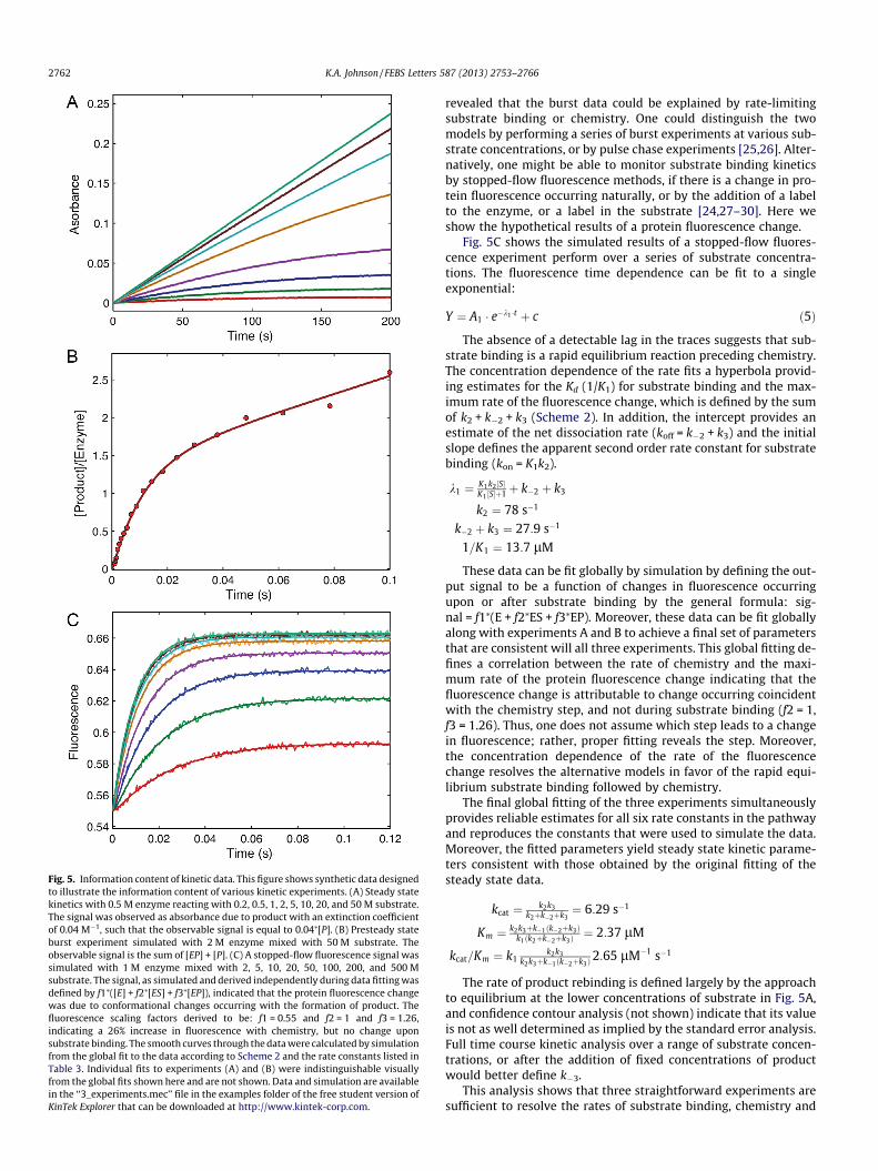
Fig. 5. Information content of kinetic data. This figure shows synthetic data designedto illustrate the information content of various kinetic experiments. (A) Steady statekinetics with 0.5 M enzyme reacting with 0.2, 0.5, 1, 2, 5, 10, 20, and 50 M substrate.The signal was observed as absorbance due to product with an extinction coefficientof 0.04 M�1, such that the observable signal is equal to 0.04⁄[P]. (B) Presteady stateburst experiment simulated with 2 M enzyme mixed with 50 M substrate. Theobservable signal is the sum of [EP] + [P]. (C) A stopped-flow fluorescence signal wassimulated with 1 M enzyme mixed with 2, 5, 10, 20, 50, 100, 200, and 500 Msubstrate. The signal, as simulated and derived independently during data fitting wasdefined by f1⁄([E] + f2⁄[ES] + f3⁄[EP]), indicated that the protein fluorescence changewas due to conformational changes occurring with the formation of product. Thefluorescence scaling factors derived to be: f1 = 0.55 and f2 = 1 and f3 = 1.26,indicating a 26% increase in fluorescence with chemistry, but no change uponsubstrate binding. The smooth curves through the data were calculated by simulationfrom the global fit to the data according to Scheme 2 and the rate constants listed inTable 3. Individual fits to experiments (A) and (B) were indistinguishable visuallyfrom the global fits shown here and are not shown. Data and simulation are availablein the ‘‘3_experiments.mec’’ file in the examples folder of the free student version ofKinTek Explorer that can be downloaded at http://www.kintek-corp.com.


revealed that the burst data could be explained by rate-limitingsubstrate binding or chemistry. One could distinguish the twomodels by performing a series of burst experiments at various sub-strate concentrations, or by pulse chase experiments [25,26]. Alter-natively, one might be able to monitor substrate binding kineticsby stopped-flow fluorescence methods, if there is a change in pro-tein fluorescence occurring naturally, or by the addition of a labelto the enzyme, or a label in the substrate [24,27–30]. Here weshow the hypothetical results of a protein fluorescence change.

Fig. 5C shows the simulated results of a stopped-flow fluores-cence experiment perform over a series of substrate concentra-tions. The fluorescence time dependence can be fit to a singleexponential:

Y ¼ A1 � e�k1 �t þ c ð5Þ

The absence of a detectable lag in the traces suggests that sub-strate binding is a rapid equilibrium reaction preceding chemistry.The concentration dependence of the rate fits a hyperbola provid-ing estimates for the Kd (1/K1) for substrate binding and the max-imum rate of the fluorescence change, which is defined by the sumof k2 + k�2 + k3 (Scheme 2). In addition, the intercept provides anestimate of the net dissociation rate (koff = k�2 + k3) and the initialslope defines the apparent second order rate constant for substratebinding (kon = K1k2).

k1 ¼ K1k2 ½S�K1 ½S�þ1þ k�2 þ k3

k2 ¼ 78 s�1

k�2 þ k3 ¼ 27:9 s�1

1=K1 ¼ 13:7 lM

These data can be fit globally by simulation by defining the out-put signal to be a function of changes in fluorescence occurringupon or after substrate binding by the general formula: sig-nal = f1⁄(E + f2⁄ES + f3⁄EP). Moreover, these data can be fit globallyalong with experiments A and B to achieve a final set of parametersthat are consistent will all three experiments. This global fitting de-fines a correlation between the rate of chemistry and the maxi-mum rate of the protein fluorescence change indicating that thefluorescence change is attributable to change occurring coincidentwith the chemistry step, and not during substrate binding (f2 = 1,f3 = 1.26). Thus, one does not assume which step leads to a changein fluorescence; rather, proper fitting reveals the step. Moreover,the concentration dependence of the rate of the fluorescencechange resolves the alternative models in favor of the rapid equi-librium substrate binding followed by chemistry.

The final global fitting of the three experiments simultaneouslyprovides reliable estimates for all six rate constants in the pathwayand reproduces the constants that were used to simulate the data.Moreover, the fitted parameters yield steady state kinetic parame-ters consistent with those obtained by the original fitting of thesteady state data.

kcat ¼ k2k3k2þk�2þk3

¼ 6:29 s�1

Km ¼ k2k3þk�1ðk�2þk3Þk1ðk2þk�2þk3Þ

¼ 2:37 lM

kcat=Km ¼ k1k2k3

k2k3þk�1ðk�2þk3Þ2:65 lM�1 s�1

The rate of product rebinding is defined largely by the approachto equilibrium at the lower concentrations of substrate in Fig. 5A,and confidence contour analysis (not shown) indicate that its valueis not as well determined as implied by the standard error analysis.Full time course kinetic analysis over a range of substrate concen-trations, or after the addition of fixed concentrations of productwould better define k�3.

This analysis shows that three straightforward experiments aresufficient to resolve the rates of substrate binding, chemistry and

http://www.kintek-corp.com

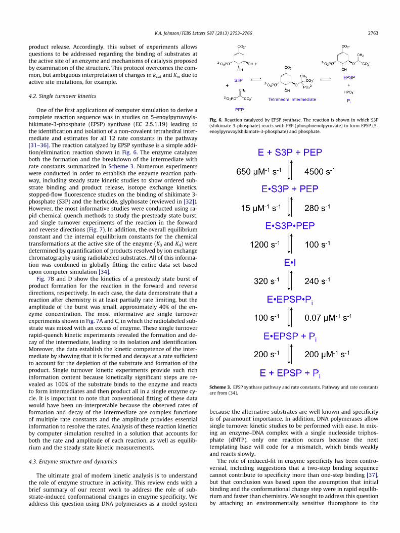
Fig. 6. Reaction catalyzed by EPSP synthase. The reaction is shown in which S3P(shikimate 3-phosphate) reacts with PEP (phosphoenolpyruvate) to form EPSP (5-enoylpyruvoylshikimate-3-phosphate) and phosphate.

Scheme 3. EPSP synthase pathway and rate constants. Pathway and rate constantsare from (34).


product release. Accordingly, this subset of experiments allowsquestions to be addressed regarding the binding of substrates atthe active site of an enzyme and mechanisms of catalysis proposedby examination of the structure. This protocol overcomes the com-mon, but ambiguous interpretation of changes in kcat and Km due toactive site mutations, for example.

4.2. Single turnover kinetics

One of the first applications of computer simulation to derive acomplete reaction sequence was in studies on 5-enoylpyruvoyls-hikimate-3-phosphate (EPSP) synthase (EC 2.5.1.19) leading tothe identification and isolation of a non-covalent tetrahedral inter-mediate and estimates for all 12 rate constants in the pathway[31–36]. The reaction catalyzed by EPSP synthase is a simple addi-tion/elimination reaction shown in Fig. 6. The enzyme catalyzesboth the formation and the breakdown of the intermediate withrate constants summarized in Scheme 3. Numerous experimentswere conducted in order to establish the enzyme reaction path-way, including steady state kinetic studies to show ordered sub-strate binding and product release, isotope exchange kinetics,stopped-flow fluorescence studies on the binding of shikimate 3-phosphate (S3P) and the herbicide, glyphosate (reviewed in [32]).However, the most informative studies were conducted using ra-pid-chemical quench methods to study the presteady-state burst,and single turnover experiments of the reaction in the forwardand reverse directions (Fig. 7). In addition, the overall equilibriumconstant and the internal equilibrium constants for the chemicaltransformations at the active site of the enzyme (K3 and K4) weredetermined by quantification of products resolved by ion exchangechromatography using radiolabeled substrates. All of this informa-tion was combined in globally fitting the entire data set basedupon computer simulation [34].

Fig. 7B and D show the kinetics of a presteady state burst ofproduct formation for the reaction in the forward and reversedirections, respectively. In each case, the data demonstrate that areaction after chemistry is at least partially rate limiting, but theamplitude of the burst was small, approximately 40% of the en-zyme concentration. The most informative are single turnoverexperiments shown in Fig. 7A and C, in which the radiolabeled sub-strate was mixed with an excess of enzyme. These single turnoverrapid-quench kinetic experiments revealed the formation and de-cay of the intermediate, leading to its isolation and identification.Moreover, the data establish the kinetic competence of the inter-mediate by showing that it is formed and decays at a rate sufficientto account for the depletion of the substrate and formation of theproduct. Single turnover kinetic experiments provide such richinformation content because kinetically significant steps are re-vealed as 100% of the substrate binds to the enzyme and reactsto form intermediates and then product all in a single enzyme cy-cle. It is important to note that conventional fitting of these datawould have been un-interpretable because the observed rates offormation and decay of the intermediate are complex functionsof multiple rate constants and the amplitude provides essentialinformation to resolve the rates. Analysis of these reaction kineticsby computer simulation resulted in a solution that accounts forboth the rate and amplitude of each reaction, as well as equilib-rium and the steady state kinetic measurements.

4.3. Enzyme structure and dynamics

The ultimate goal of modern kinetic analysis is to understandthe role of enzyme structure in activity. This review ends with abrief summary of our recent work to address the role of sub-strate-induced conformational changes in enzyme specificity. Weaddress this question using DNA polymerases as a model system

because the alternative substrates are well known and specificityis of paramount importance. In addition, DNA polymerases allowsingle turnover kinetic studies to be performed with ease. In mix-ing an enzyme–DNA complex with a single nucleoside triphos-phate (dNTP), only one reaction occurs because the nexttemplating base will code for a mismatch, which binds weaklyand reacts slowly.

The role of induced-fit in enzyme specificity has been contro-versial, including suggestions that a two-step binding sequencecannot contribute to specificity more than one-step binding [37],but that conclusion was based upon the assumption that initialbinding and the conformational change step were in rapid equilib-rium and faster than chemistry. We sought to address this questionby attaching an environmentally sensitive fluorophore to the

Fig. 7. EPSP presteady-state and single turnover kinetics. (A) Single turnover in the forward direction. (B) Presteady state burst in the forward direction. (C) Single turnover ofthe reaction in the reverse direction. (D) Presteady state burst in the reverse direction. The inset to each figure gives the starting concentration of reach reactant, and thespecies shown in red contains the radiolabel. Redrawn with permission from [34]. The smooth lines were calculated by simulation according to the pathway and rateconstants given in Scheme 3. Data and simulations are available in the ‘‘EPSP.mec’’ KinTek Explorer example file.


nucleotide recognition domain of HIV reverse transcriptase (HIVreverse transciptase (HIVRT), EC 2.7.7.49) as shown in Fig. 8[24,38]. Positioned on the surface of the protein, the fluorescent la-bel does not perturb the kinetics of the reaction, but provides a sig-nal to monitor changes in protein structure from open to closedstates after binding nucleotide.

The results of one experiment are shown in Fig. 9A. After mixingTTP with an HIVRT–DNA complex, there is a decrease in fluores-cence followed by an increase, representing a single turnover inwhich the enzyme binds substrate, closes, catalyzes chemistryand then opens. Fig. 9B shows the results of a rapid-quench flowexperiment to monitor the time dependence of the chemical reac-tion. Fitting both curves simultaneously demonstrates that theslow rise of the fluorescence transient is coincident with the rateof the chemical reaction, implying fast opening after chemistry.In studies not shown, the binding of TTP to an enzyme–DNAdd

complex (where the DNA was terminated by a dideoxynucleotideto prevent chemistry) the fluorescence decreased rapidly in form-ing the closed E-DNAdd–TTP complex, corresponding to that seenby crystallography [24,39]. Finally, an experiment was done tomeasure the release of bound TTP from a pre-formed E-DNAdd–TTP complex (Fig. 9C). After mixing with an excess of unlabeledE-DNA complex, there is an increase in fluorescence providing ameasurement of the rate of enzyme opening to release TTP. Thesethree experiments were fit globally to derive the pathway shownin Scheme 4, where ED and FD represent the open and closed statesof the enzyme–DNA complex, respectively.

Surprisingly, because the rate of TTP release is slow relative tochemistry, the specificity constant for the enzyme is equal to the

second order rate constant for substrate binding, determined bythe initial weak substrate binding and the rate of the conforma-tional change.

kcat=Km ¼ K1k2 ¼ 7:5 lM�1s�1

kcat ¼ k3 ¼ 34 s�1

Km ¼ kcatkcat=Km

� k3K1k2¼ 4:7 lM

Kd;net ¼ 1=K1ð1þ K2Þ ¼ 0:4 lM

The rate of chemistry cancels from the expression for kcat/Km be-cause k3 is in both the numerator and denominator. Moreover, Km

is determined by the ratio of kcat and the substrate binding rate(K1k2). Contrary to previous theories, these results indicate thatthe substrate-induced conformational change is a major determi-nant of enzyme specificity. The specificity constant for correctnucleotide incorporation is governed by the nucleotide affinity inthe initial weak binding to the open state and the rate of the con-formational change to form the closed state. This unexpected resultimplies that specificity is determined by the most ephemeral ofstates that are most difficult to study directly, the initial weakbinding and the rate of the conformational change. Therefore, inorder to understand the molecular details underlying the sub-strate-induced conformational change, we have followed up thesestudies by extensive molecular dynamics simulations [40]. Thesesimulations accurately predict the rates of the conformationalchange in the forward and reverse directions and reveal new de-tails at atomic resolution.

Much of the debate regarding the role of induced fit in enzymespecificity over the past few decades was due to the lack of

Fig. 8. Structure of fluorescently labeled HIVRT. The structure of HIVRT wasrendered in pymol from 1rtd.pdb [39]. The position of the fluorescent label(magenta spheres) was docked at the position of the E36C substitution [24]. DuplexDNA is in blue (template) and green (primer), while the incoming nucleotide ismagenta (sticks).

Fig. 9. HIVRT kinetics. (A) Fluorescently labeled HIVRT in complex with duplex DNA(200 nM MDCC-labeled HIVRT with 300 nM DNA) was mixed with variousconcentrations of TTP (2, 4, 10, 20, 40, 60, 80, and 100 M) in a stopped-flow andthe time course of fluorescence was recorded. (B) Rapid quench-flow methods wereused to measure the time dependence of the chemical reaction after mixing theHIVRT–DNA complex (150 nM MDCC-labeled HIVRT with 100 nM DNA) withvarious concentrations of TTP (0.25, 0.5, 2, 10, 25, and 100 M). Redrawn withpermission from [38]. Smooth curves show the global fit to all of the date accordingto Scheme 4.


definitive data. Steady state kinetic analysis could not resolve theissue and so theoretical arguments abounded. Single turnoverkinetic studies provided the direct measurement of events that dic-tate the fate of substrate after the initial binding step and therebydefine the molecular events that determine specificity.

5. Summary

Here I have provided a brief history of enzyme kinetics from itsbeginnings a century ago to modern applications of kinetic analysisof enzyme reaction pathways that are made possible by the use oftransient-state kinetic methods and computer-based data fittingroutines. I have only hit some of the highlights of advances inkinetic data analysis over the last few decades using examplesfrom my own lab. Certainly many others have contributed impor-tant, insightful and instructive examples that could have easilyillustrated major advances in methods of analysis and informationto define enzyme catalysis. For example, I have not discussed theuse of singular value decomposition (SVD) to deconvolute time-re-solved spectra, which is certainly an important technical advance[41]. In recent collaborative work, we have simultaneously fit,stopped-flow fluorescence transients, rapid-quench-flow data,and SVD analysis of time resolve absorbance measurements todeduce a unique branched enzyme pathway [42].

It is interesting to note that the constant derived by Michaelisand Menten in the analysis of the full time course kinetics wasnot the Michaelis constant, but rather, Vmax/Km. In some sense itwas a historical accident to define the steady state equation interms of kcat and Km values, resulting in confusion over the inter-pretation of Km. Because of the importance of kcat/Km in determin-ing enzyme specificity, efficiency and proficiency [43], it wouldhave been better if the equation had been defined in terms of thetwo primary constants, kcat and ‘‘kcat/Km’’, such that Km was simplythe ratio of the two.

Scientists and historians often dream of time travel. In thisbrief review of the history of enzyme kinetic data analysis, it isamusing to think of what Leonor Michaelis and Maud Mentenwould think of our current methods of data analysis. No doubtthey would be astounded at how the click of a computer mousecan trigger millions of calculations to be completed in secondsto find an optimal global fit involving a rather complex kineticmodel and multiple data sets, or that molecular dynamics simu-lations of the motions of atoms could predict the moleculardetails of reactions governing enzyme specificity. Nonetheless,

they would be justifiably proud of their accomplishments andpleased at how their work has stood the test of such advancedcomputational analysis. It is now our turn to ponder the newdiscoveries of the next century and wonder whether our workwill stand the test of new scientific advances.

Scheme 4. HIV reverse transcriptase pathway and rate constants. EDn represents the enzyme-DNA complex with a primer n nucleotides in length; N, nucltleosidetriphosphate, PPi, pyrophosphate. From (38).


Financial Conflict of Interest

K.A. Johnson is the President of KinTek Corporation, which sellslicenses for a professional version of KinTek Explorer software andinstruments for transient kinetic analysis.

Acknowledgment

Supported by the Welch Foundation grant F-1604 and NIHgrant GM044613.

References

[1] Michaelis, L. and Menten, M.L. (1913) Die Kinetik der Invertinwirkung.Biochemische Zeitschrift 49, 333–369.

[2] Johnson, K.A. and Goody, R.S. (2011) The original Michaelis constant:translation of the 1913 Michaelis–Menten paper. Biochemistry 50, 8264–8269.

[3] Goody, R.S. and Johnson, K.A. () The kinetics of inverase action: translation of1913 paper by Leonor Michaelis and Maud Menten. Biochemistry. http://pubs.acs.org/doi/suppl/10.1021/bi201284u.

[4] Sainz-Polo, M.A., Ramirez-Escudero, M., Lafraya, A., Gonzalez, B., Marin-Navarro, J., Polaina, J. and Sanz-Aparicio, J. (2013) Three-dimensional structureof Saccharomyces invertase: role of a non-catalytic domain in oligomerizationand substrate specificity. J. Biol. Chem. 288, 9755–9766.

[5] Henri, V. (1903) Lois générales de l’action des diastases, Hermann, Paris.[6] Briggs, G.E. and Haldane, J.B. (1925) A note on the kinetics of enzyme action.

Biochem. J. 19, 338–339.[7] Hasselbalch, K.A. (1917) Die Berechnung der Wasserstoffzahl des Blutes aus

der freien und gebundenen Kohlensäure desselben, und die Sauerstoffbindungdes Blutes als Funktion der Wasserstoffzahl. Biochemische Zeitschrift 78, 112–144.

[8] Lineweaver, H. and Burk, D. (1934) The determination of enzyme dissociationconstants. J. Am. Chem. Soc. 56, 658–666.

[9] Hofstee, B.H. (1959) Non-inverted versus inverted plots in enzyme kinetics.Nature 184, 1296–1298.

[10] Dowd, J.E. and Riggs, D.S. (1965) A comparison of estimates of Michaelis–Menten kinetic constants from various linear transformations. J. Biol. Chem.240, 863–869.

[11] Johnson, K.A., Simpson, Z.B. and Blom, T. (2009) FitSpace explorer: analgorithm to evaluate multidimensional parameter space in fitting kineticdata. Anal. Biochem. 387, 30–41.

[12] Johnson, K.A., Simpson, Z.B. and Blom, T. (2009) Global kinetic explorer: a newcomputer program for dynamic simulation and fitting of kinetic data. Anal.Biochem. 387, 20–29.

[13] Golicnik, M. (2013) The integrated Michaelis-Menten rate equation: deja vu orvu jade? J Enzyme Inhib Med Chem. 28, 879–893.

[14] Kuzmic, P. (1996) Program DYNAFIT for the analysis of enzyme kinetic data:application to HIV proteinase. Anal. Biochem. 237, 260–273.

[15] Barshop, B.A., Wrenn, R.F. and Frieden, C. (1983) Analysis of numericalmethods for computer simulation of kinetic processes: development ofKINSIM – a flexible, portable system. Anal. Biochem. 130, 134–145.

[16] Bates, D.M. and Watts, D.G. (1988) Nonlinear Regression Analysis and itsApplications, John Wiley & Sons, New York.

[17] Spies, M.A., Woodward, J.J., Watnik, M.R. and Toney, M.D. (2004) Alanineracemase free energy profiles from global analyses of progress curves. J. Am.Chem. Soc. 126, 7464–7475.

[18] Press, W.H., Vetterling, W.T. and Flannery, B.P. (2007) Numerical Recipies inC++, third ed, Cambridge University Press, New York.

[19] Segel, I.R. (1975) Enzyme kinetics: Behavior and Analysis of Rapid Equilibriumand Steady-State Enzyme Systems, John Wiley & Sons, New York.

[20] Dixon, M. and Webb, E.C. (1979) Enzymes, third ed, Academic Press, New York.[21] Cornish-Bowden, A. (2012) Fundamentals of Enzyme Kinetics, fourth ed,

Wiley-VCH Verlag & Co., Weinheim, Germany.[22] Johnson, K.A. (1995) Rapid quench kinetic analysis of polymerases,

adenosinetriphosphatases, and enzyme intermediates. Methods Enzymol.249, 38–61.

[23] Johnson, K.A. (1992) Transient-state kinetic analysis of enzyme reactionpathways. The Enzymes XX, 1–61.

[24] Kellinger, M.W. and Johnson, K.A. (2010) Nucleotide-dependentconformational change governs specificity and analog discrimination by HIVreverse transcriptase. Proc. Natl. Acad. Sci. USA 107, 7734–7739.

[25] Johnson, K.A. and Porter, M.E. (1982) Transient state kinetic analysis of thedynein ATPase. Prog. Clin. Biol. Res. 80, 101–106.

[26] Johnson, K.A. and Taylor, E.W. (1978) Intermediate states of subfragment 1and actosubfragment 1 ATPase: reevaluation of the mechanism. Biochemistry17, 3432–3442.

[27] Tsai, Y.C., Jin, Z. and Johnson, K.A. (2009) Site-specific labeling of T7 DNApolymerase with a conformationally sensitive fluorophore and its use indetecting single-nucleotide polymorphisms. Anal. Biochem. 384, 136–144.

[28] Tsai, Y.C. and Johnson, K.A. (2006) A new paradigm for DNA polymerasespecificity. Biochemistry 45, 9675–9687.

[29] Gilbert, S.P., Moyer, M.L. and Johnson, K.A. (1998) Alternating site mechanismof the kinesin ATPase. Biochemistry 37, 792–799.

[30] John, J., Sohmen, R., Feuerstein, J., Linke, R., Wittinghofer, A. and Goody, R.S.(1990) Kinetics of interaction of nucleotides with nucleotide-free H-ras p21.Biochemistry 29, 6058–6065.

[31] Anderson, K.S. and Johnson, K.A. (1990) ‘‘Kinetic competence’’ of the 5-enolpyruvoylshikimate-3-phosphate synthase tetrahedral intermediate. J.Biol. Chem. 265, 5567–5572.

[32] Anderson, K.S. and Johnson, K.A. (1990) Kinetic and structural analysis ofenzyme intermediates: lessons from EPSP synthase. Chem. Rev. 90, 1131–1149.

[33] Anderson, K.S., Sammons, R.D., Leo, G.C., Sikorski, J.A., Benesi, A.J. andJohnson, K.A. (1990) Observation by 13C NMR of the EPSP synthasetetrahedral intermediate bound to the enzyme active site. Biochemistry29, 1460–1465.

[34] Anderson, K.S., Sikorski, J.A. and Johnson, K.A. (1988) A tetrahedralintermediate in the EPSP synthase reaction observed by rapid quenchkinetics. Biochemistry 27, 7395–7406.

[35] Anderson, K.S., Sikorski, J.A. and Johnson, K.A. (1988) Evaluation of 5-enolpyruvoylshikimate-3-phosphate synthase substrate and inhibitorbinding by stopped-flow and equilibrium fluorescence measurements.Biochemistry 27, 1604–1610.

[36] Anderson, K.S., Sikorski, J.A., Benesi, A.J. and Johnson, K.A. (1988) Isolation andstructural elucidation of the tetrahedral intermediate in the EPSP synthasereaction pathway. J. Am. Chem. Soc. 110, 6577–6579.

[37] Fersht, A.R. (1999) Enzyme Structure and Mechanism, third ed, Freeman, NewYork.

[38] Kellinger, M.W. and Johnson, K.A. (2011) Role of induced fit in limitingdiscrimination against AZT by HIV reverse transcriptase. Biochemistry 50,5008–5015.

[39] Huang, H.F., Chopra, R., Verdine, G.L. and Harrison, S.C. (1998) Structure of acovalently trapped catalytic complex of HIV-I reverse transcriptase:implications for drug resistance. Science 282, 1669–1675.

[40] Kirmizialtin, S., Nguyen, V., Johnson, K.A. and Elber, R. (2012) Howconformational dynamics of DNA polymerase select correct substrates:experiments and simulations. Structure 20, 618–627.

[41] Henry, E.R. and Hofrichter, J. (1992) Singular value decomposition: applicationto analysis of experimental data. Methods Enzymol. 210, 129–192.

[42] Schroeder, G.K., Johnson Jr., W.H., Huddleston, J.P., Serrano, H., Johnson, K.A.and Whitman, C.P. (2012) Reaction of cis-3-chloroacrylic acid dehalogenasewith an allene substrate, 2,3-butadienoate: hydration via an enamine. J. Am.Chem. Soc. 134, 293–304.

[43] Miller, B.G. and Wolfenden, R. (2002) Catalytic proficiency: the unusual case ofOMP decarboxylase. Annu. Rev. Biochem. 71, 847–885.

http://refhub.elsevier.com/S0014-5793(13)00527-9/h0005





http://pubs.acs.org/doi/suppl/10.1021/bi201284u

http://pubs.acs.org/doi/suppl/10.1021/bi201284u










































































































a century of enzyme kinetic analysis, 1913 to 2013 a century of enzyme kinetic analysis, 1913 to...

Documents