a can based distributed telemetry and telecommand network
TRANSCRIPT

A CAN Based Distributed Telemetry and Telecommand Network for a Nanosatellite
Simphiwe Khumalo
Thesis presented in partial fulfillment of the requirements for the degree of Master of Science in Electronic Engineering
at the University of Stellenbosch Electrical and Electronic Engineering Department
Supervisors: Professor W.H Steyn and Mr. A. Barnard
March 2008

Copyright ©2008 Stellenbosch University All rights reserved

i
Declaration
I, the undersigned, hereby declare that the work contained in this thesis is my own original work and that I have not previously in its entirety or in part submitted it at any university for a degree.
Signature: ........................................ Date: ...................................

ii
Abstract
A communications protocol is designed for real time control and data handling for a
Nanosatellite application. The communication protocol is based on the Controller Area
Network (CAN) technology. The protocol handles different message types such as time
synchronization, telecommand messages, telemetry acquisition, unsolicited telemetry
messages, large file transfers and debug messages.
The design of the protocol entails finding a suitable target microcontroller in which the
protocol implementation is demonstrated. This requires consideration of a number of
development factors such as cost, complexity, availability, reliability and operational
environment (space). The AVR AT90CAN128 microcontroller was chosen as a target
microcontroller as it gave most of the required factors mentioned above.
The protocol implementation involves developing low level software drivers, the middleware
and the application programs to demonstrate handling of each supported message. In the
implementation the media access scheme and low layer communication is provided by the
CAN low level kernel (physical and data link layers).
The protocol performance was evaluated by measuring the software response latencies, the
bus throughputs and the software efficiencies. Power consumption due to CAN
communication was also measured.
System reliability was tested by loading the CAN bus with extreme communication traffic
and letting the system run for a long time. The observation was that messages were handled
consistently.
iii
Opsomming
’n Kommunikasie protokol is ontwerp vir die intydse beheer en data hantering vir ’n
Nanosateliet toepassing. Die kommunikasie protokol is gebaseer op die “Controller Area
Network” (CAN) tegnologie. Die kommunikasie protokol hanteer verskillende boodskappe
soos tydsinkronisasie, afstandsbevel, telemetrie aanvraag, ongevraagde telemetrie, groot lêer
oordragte en ontfoutings boodskappe.
Die ontwerp van die protokol behels die vind van ’n geskikte mikrobeheerder waarop die
protokol gedemonstreer kan word. Dit behels die inagneming van verskeie faktore soos koste,
kompleksiteit, beskikbaarheid, betroubaarheid asook die operasionele omgewing (ruimte).
Die AVR AT90CAN128 mikrobeheerder was gekies aangesien dit aan meeste van die
voorafgenoemde vereistes voldoen.
Die implementering van die protokol behels die ontwikkeling van lae vlak sagteware drywers,
die tussenware en die toepassing programmatuur om die hantering van die ondersteunde
boodskappe te demonstreer. In hierdie implementasie word die media toegangsskema en lae
vlak kommunikasie verskaf deur die CAN lae vlak kern ( Fisiese kant data koppel vlakke).
Die protokol se doeltreffenheid was geëvalueer deur die sagteware se reaksietyd, die bus
deurset en sagteware effektiwiteit te meet. Die drywingsverbruik as gevolg van die CAN
kommunikasie is ook gemeet.
Stelsel integriteit is getoets deur die CAN bus swaar te belaai en die stelsel vir lang,
aaneenlopende periodes van tyd te laat loop. Dit is bevind dat die boodskappe konsekwent
hanteer is.

iv
Acknowledgements
I would like to thank the following people and institutions, on their shoulders I stand:
• I dedicate this work to my Lord, Jesus Christ, for guidance, wisdom, strength and
inspiration.
• The financial assistance of the National Research Foundation (NRF) and Department of
Science & Technology (DST) towards this research is hereby acknowledged.
• My Supervisors: You are the custodians of your practice.
• My family: You trusted my abilities and gave me support.
• All my colleagues: Your company encouraged me.

Table of Contents
Abstract ...................................................................................................................................... ii
Opsomming ...............................................................................................................................iii
Acknowledgements ................................................................................................................... iv
Table of Contents ....................................................................................................................... v
List of Figures ............................................................................................................................ x
List of Tables............................................................................................................................xii
List of Acronyms.....................................................................................................................xiii
Chapter 1................................................................................................................................... 1
Background............................................................................................................................... 1
1.1 Introduction .................................................................................................................... 1
1.2 Project Objectives .......................................................................................................... 2
1.3 Standard Communication Bus Protocols........................................................................ 3
1.3.1 Inter-Integrated Circuit (I2C) Interface .......................................................................... 4
1.3.2 Serial Peripheral Interface (SPI) .................................................................................... 4
1.3.3 Microwire ....................................................................................................................... 5
1.3.4 Controller Area Network (CAN).................................................................................... 5
1.3.5 Process Field Bus (Profibus) .......................................................................................... 6
1.4 A preferred Communications Bus and Motivation ........................................................ 7
1.5 Review of Higher Layer Application Protocols (HLP).................................................. 9
1.5.1 Previous CAN-Protocol Developments in the ESL....................................................... 9

Contents
vi
1.5.2 Commercial Higher Layer Application Protocols........................................................ 11
1.5.2.1 CANopen................................................................................................................... 11
1.5.2.2 DeviceNet................................................................................................................. 15
1.6 Thesis Overview........................................................................................................... 20
Chapter 2................................................................................................................................. 22
The CAN Protocol Conceptual System Design.................................................................... 22
2.1 Supporting Hardware Consideration............................................................................ 22
2.1.1 Choosing a Target Microcontroller .............................................................................. 23
2.1.2 The Other Supporting Components.............................................................................. 26
2.1.3 Bus Architecture Overview.......................................................................................... 26
2.2 The Protocol Design Consideration ............................................................................. 28
2.2.1 The CAN Identifier Assignment .................................................................................. 28
2.2.2 Message Handling and Prioritization ........................................................................... 30
2.3 Timing Analysis ........................................................................................................... 37
Chapter 3................................................................................................................................. 39
Detailed Design and Protocol Implementation.................................................................... 39
3.1 The software structure.................................................................................................. 39
3.1.1 CAN interrupt Handling............................................................................................... 42
3.1.2 Node Initialization & configuration ............................................................................. 44
3.1.3 System Control and Reset ............................................................................................ 45
3.1.4 System Timing ............................................................................................................. 46
3.2 Subsystem Level Message Handling............................................................................ 47

Contents
vii
3.2.1 Subsystem Telemetry Acquisition ............................................................................... 47
3.2.2 Subsystem Telecommand Handling............................................................................. 49
3.2.3 Data Transfers .............................................................................................................. 50
3.2.4 Debug Messages........................................................................................................... 54
Chapter 4................................................................................................................................. 55
Protocol Performance and Implementation Results ........................................................... 55
4.1 Hardware Performance Measurements ........................................................................ 55
4.2 Software Time Response.............................................................................................. 56
4.2.1 Main Loop Execution Time Response......................................................................... 58
4.3 Bus Throughput and Protocol Software Efficiency..................................................... 60
4.4 Software Reliability...................................................................................................... 62
Chapter 5................................................................................................................................. 64
Conclusion and Recommendations....................................................................................... 64
5.1 Conclusion.................................................................................................................... 64
5.2 Recommendations ........................................................................................................ 66
Bibliography ........................................................................................................................... 68
Appendix A ................................................................................................................................ i
Controller Area Network - CAN Information........................................................................ i
A.1 What is CAN? ................................................................................................................. i
A.2 CAN standards ................................................................................................................ i
A.3 How CAN works? .......................................................................................................... ii
A.3.1 Principle ......................................................................................................................... ii

Contents
viii
A.3.2 Identifiers & arbitration.................................................................................................. ii
A.3.3 Remote frames...............................................................................................................iii
A.3.4 Message formats............................................................................................................iii
A.3.4.1 Format of a CAN message ........................................................................................iii
A.3.4.2 CAN 2.0A Format ..................................................................................................... iv
A.3.4.3 CAN 2.0B Format ...................................................................................................... v
A.3.5 Error detection and fault confinement........................................................................... vi
A.3.5.1 The CAN error process ............................................................................................. vi
A.3.5.2 Error detection........................................................................................................... vi
A.3.5.3 CAN controller error modes.....................................................................................vii
A.3.5.4 Error signaling.........................................................................................................viii
A.3.6 Bit timing....................................................................................................................... ix
A.3.6.1 Bit segments .............................................................................................................. ix
A.3.6.2 Synchronization segment (Synch_Seg).................................................................... ix
A.3.6.3 Propagation segment (Prop_Seg) ............................................................................. ix
A.3.6.4 Phase Segment 1 (Phase_Seg1), Phase Segment 2 (Phase_Seg2) ............................. x
A.3.7 Resynchronization.......................................................................................................... x
A.3.7.1 Hard resynchronization .............................................................................................. x
A.3.8 CAN bus physical layer.................................................................................................. x
A.3.8.1 ISO 11898.................................................................................................................. xi
A.3.8.2 ISO 11519.................................................................................................................. xi
A.3.9 Bus lengths ...................................................................................................................xii

Contents
ix
A.3.10 Media.........................................................................................................................xii
A.3.11 CAN implementations...............................................................................................xii
Appendix B............................................................................................................................. xvi
CAN Baud Rate Setting ........................................................................................................ xvi
Appendix C ............................................................................................................................. xx
Source Code ............................................................................................................................ xx
canprotocol_main.c ................................................................................................................. xxi
can_msg_drv.c........................................................................................................................xxii
candriv.c ................................................................................................................................xxiii
canTimer.c............................................................................................................................. xxiv
adc_mlib.c .............................................................................................................................. xxv
sensor_drv. ............................................................................................................................ xxvi
canDemo.c............................................................................................................................xxvii

x
List of Figures
Figure 1.1: CAN Bus Setup for A Typical Satellite................................................................ 3
Figure 1.2: SPI Communication Scheme ................................................................................ 4
Figure 1.3: Proposed CAN 11-Bit Frame.............................................................................. 10
Figure 1.4: CANopen OSI Model ......................................................................................... 13
Figure 1.5: CANopen device bus Interface........................................................................... 15
Figure 1.6: CANopen 11-bit ID-Distribution........................................................................ 15
Figure 1.7: DeviceNet Topology........................................................................................... 16
Figure 1.8: DeviceNet Layer Model ..................................................................................... 17
Figure 1.9: A CAN Module Schematic................................................................................. 20
Figure 2.1: SRAM Data Memory Map ................................................................................. 25
Figure 2.2: Program Memory Map ....................................................................................... 26
Figure 2.3: A Terminated CAN Bus Architecture ................................................................ 27
Figure 2.4: A 29-Bit ID Allocation ....................................................................................... 28
Figure 2.5: A Telecommand Exchange................................................................................. 32
Figure 2.6: Unsolicited Telemetry Format............................................................................ 33
Figure 2.7: File Transfer Flow Diagram Example ................................................................ 36
Figure 2.8: Data Throttling Mechanism................................................................................ 36
Figure 2.9: A typical Debug Message................................................................................... 37
Figure 3.1: A CAN/OSI Reference model ............................................................................ 39
Figure 3.2: Protocol Software Modules ................................................................................ 41

Figures
xi
Figure 3.3: Protocol Software Structure................................................................................ 41
Figure 3.4: CAN Interrupt Structure ..................................................................................... 43
Figure 3.5: CAN Interrupt Flow Diagram............................................................................. 44
Figure 3.6: Code Upload Diagram ........................................................................................ 52
Figure 3.7: Code Segment Update and Code Upload ........................................................... 53
Figure 4.1: System Test Setup............................................................................................... 55
Figure 4.2: Main Function Flow Diagram ............................................................................ 59
Figure 4.3: CAN Bus Throughput......................................................................................... 62
Figure A.1: CAN Version 2.0A Message Frame .................................................................... iv
Figure A.2: CAN 2.0B Message Format................................................................................. vi
Figure A.3: CAN Error States ...............................................................................................viii
Figure A.4: CAN Bit Timing ................................................................................................. ix

xii
List of Tables
Table 1.1: Serial Bus Comparison........................................................................................... 9
Table 1.2: 1DeviceNet Identifier Distribution ....................................................................... 19
Table 2.1: Microcontroller Comparison................................................................................ 22
Table 2.2: AT90CAN128 Memory Mapping........................................................................ 24
Table 2.3: The Protocol Supported Message Types.............................................................. 29
Table 2.4: Standard Telecommand Channels........................................................................ 31
Table 2.5: Standard Telemetry Channels .............................................................................. 33
Table 4.1: Message Latencies ............................................................................................... 57
Table 4.2: Main Loop Execution Time ................................................................................. 59
Table 4.3: Throughputs and Efficiencies .............................................................................. 61
Table A.1: CAN Bus Voltage Levels..................................................................................... xi
Table A.2: CAN Bus Voltage Levels..................................................................................... xi
Table A.3: Practical Maximum Bus Lengths ........................................................................xii
Table A.4: BasicCAN features............................................................................................. xiv
Table A.5: FullCAN features ................................................................................................ xv

xiii
List of Acronyms
A/D Analog to Digital ACK Acknowledgement ARM Advanced RISC Machine ADCS Attitude Determination and Control System CAN Controller Area Network CAN_H CAN High CAN_L CAN Low CAL CAN Application Layer CiA CAN in Automation CIP Control and Information Protocol CLK Clock CMD Command CHL Channel DSP Digital Signal Processing EEPROM Electrical Erasable Programmable Read Only Memory GPS Global Positioning System HLP Higher Layer Protocol I/O Input/Output ID Identifier IDX Index ISO International Standardization Organization JTAG Joint Test Action Group LSB Least Significant Bit MAC Media Access Control MMU Mass Memory Unit MSB Most Significant Bit OBC On-Board Computer OSI Open Systems Interconnection PCAN PEAK CAN Applications PCI Peripheral Connection Interface PROFIBUS Process Field Bus RISC Reduced Instruction Set RF Radio Frequency SP Stack Pointer SUNSAT Stellenbosch University Satellite TLM Telemetry TLCMD Telecommand

1
Chapter 1
Background
1.1 Introduction
The development of satellite applications has evolved over the years and the continuous use
of this technology has expanded over a wide range of applications including communications,
guidance and navigation systems, military and defense, academic research etc. Satellite
development has evolved from large earth orbiting satellites (greater than 1000 kilograms) to
nanosatellites (less than 10 kilograms) and even smaller femtosatellites (less than 0.1
kilograms). Nanosatellites are commonly developed by universities and the research institutes
for research or academic purposes.
One of possibly the most complex satellite projects ever attempted by university students was
the Stellenbosch University Satellite (SUNSAT) [2]. The research in satellite engineering has
since SUNSAT been going on at the University of Stellenbosch and a suitable environment
for this type of research was established when the Electronic Systems Laboratory (ESL) was
formed in 1991 at the Electrical and Electronic Engineering Department. Using the experience
and the tools developed in the ESL, the research project reported in this document was
formulated to develop a communications bus and protocol for a Nanosatellite.
In realizing the successful development of this project a brief study was done on various
existing field bus protocols. However, this study focuses on the Controller Area Network
(CAN) as the preferable candidate, since previous satellite developments used CAN bus
successfully and that provides for a space tested technology. The CAN bus was chosen for
various other reasons that will be discussed in the next subsections.
The bus protocol in this project was designed and developed completely for a Nanosatellite,
but it is generic enough to be customized and used in any satellite mission. Though
commercial high layer application protocols, like CANopen, DeviceNet and CANKingdom
could be used, selecting a suitable communication protocol to support a specific application
requires an understanding of both the protocol and the application. Whether generic or
application-specific, a commercial protocol will probably limit the optimization of the system.

CHAPTER 1. BACKGROUND
2
This optimization may be crucial in applications with tight performance, cost, size, weight,
and environmental constraints [3].
A literature survey is done in the following subsections to evaluate whether to design and
develop a generic communication bus protocol or to customize the commercial higher layer
application protocols like CANopen, DeviceNet and CANKingdom for a nanosatellite
application.
1.2 Project Objectives
The primary objective of this project was to design a very basic, efficient, highly reliable and
robust communication protocol for a Nanosatellite application. The protocol is robust if it can
quickly detect and recover from errors with a high degree of certainty. The protocol efficiency
is quantified by the data delivered, compared to the raw network bandwidth [12]. The
protocol reliability is measured by the basic merits to handle extreme communication traffic
under extreme environmental conditions consistently.
The protocol should handle all the communications in real time and it should also handle
scheduled messages timely to be executed periodically depending on the application. An
auxiliary objective will be to demonstrate the protocol implementation on a cost effective, low
power microcontroller supporting the chosen communications bus.
An overall objective was to develop a protocol that will facilitate the communication among
all the Nanosatellite subsystems as shown in figure 1.1. The CAN bus will be the main
communications bus, but a private direct communication between certain nodes can be
implemented using any of the serial bus interface that is seen convenient for the specific
application. For example, the Onboard Computer (OBC) has direct access to the Mass
Memory Unit (MMU) using a Serial Peripheral Interface (SPI) standard as shown in figure
1.1.

CHAPTER 1. BACKGROUND
3
Figure 1.1: CAN Bus Setup for A Typical Satellite
1.3 Standard Communication Bus Protocols
In order to carry out the objectives as set out for this project, a very brief survey was done on
the standard protocols for distributed applications. Most of the protocols studied were
characterized as primarily addressing three levels of protocol standardization and these levels
are [12]:
• Medium Access Control (MAC): this low level sub-layer defines the bus sharing and
arbitration layer that is a fundamental part of every communication network. The reduction in
the complexity of the related wiring harness is determined by this part of the communications
protocol.
• Protocol Implementation: this consists of the development of software drivers and
hardware interfacing for the realization of the desired application. This level must suit the
application and it must offer most features that are required for a simplified protocol
implementation. The CAN bus specification provides most of these features.
• High level Application Standards: this level represents the element of the protocol
that provides cohesion between the applications components e.g. sensors, actuators and the
application software. It also provides interoperability between the nodes in a network.
Based on the protocol characterization mentioned above and other factors, including cost,
availability and complexity, the communication bus standards discussed in the next section
were considered. However, it should be noted there is a large number of other

CHAPTER 1. BACKGROUND
4
communications bus standards that can be possible candidates, but only those that presented
attractive features were considered here.
1.3.1 Inter-Integrated Circuit (I 2C) Interface
The I2C bus is a half-duplex, synchronous, multi-master bus requiring only two signal wires:
Data (SDA) and Clock (SCL) [16].
I2C uses an addressable communications protocol that allows the master to communicate with
individual slaves using a 7-bit (standard mode) or 10-bit (High Speed mode) address.
The I2C bus has three speeds: slow (less than 100Kbps), fast (400Kbps), and high-speed
(3.4Mbps), each downward compatible. The true limit to I2C link distances is the bit-rate and
a bus capacitance of 400 picoFarads (pF).
1.3.2 Serial Peripheral Interface (SPI)
The SPI bus consists of four signals: master out slave in (MOSI), master in slave out (MISO),
serial clock (SCK), and active-low slave select (/SS). As a multi-master/slave protocol,
communication between the master and selected slave uses the unidirectional MISO and
MOSI lines, to achieve data rates over 1Mbps in full duplex mode. The data is clocked
simultaneously into the slave and master based on the SCK pulses, provided by the master
[16].
The SPI bus employs a simple shift register data transfer scheme: Data is clocked out of and
into the active devices in a first-in, first-out fashion [FIFO] [17]. SPI devices can transmit and
receive data packets in full duplex mode and the communication scheme is shown in figure
1.2.
Figure 1.2: SPI Communication Scheme
CHAPTER 1. BACKGROUND
5
Data transfers are performed in eight/sixteen bit blocks. All data transfer is synchronized by
the serial clock (SCLK).
A disadvantage of SPI is the requirement to have separate /SS lines for each slave due to its
lack of built-in addressing, resulting in an increased complexity in connectivity as the number
of slaves increases. Provided that extra I/O pins are available, or extra board space for de-
multiplexer electronics, this may not be a problem. For small, low-pin-count microcontrollers,
a multi-slave SPI interface might not be a viable solution [17].
1.3.3 Microwire
Microwire is a 4-wire synchronous bus interface developed by National Semiconductor [18].
Similar to SPI, Microwire is a master/slave bus interface, with serial data out of the master
(SO), and serial data in to the master (SI), and a signal clock (SK). These correspond to SPI's
MOSI, MISO, and SCK signals, respectively. There is also a chip select signal, which acts
similarly to SPI's /SS lines. As a full-duplex bus, Microwire is capable of speeds up to
625Kbps or slower (bus capacitance dependant).
Microwire devices come with different protocol standards, based on their data needs. Unlike
SPI, which is based on one byte or two bytes data packets, Microwire permits a variable data
length packet.
Microwire has the same advantages and disadvantages as SPI with respect to multiple slaves,
which require multiple chip select lines. In some instances, a SPI device will work on a
Microwire bus, as will a Microwire device work on a SPI bus, although this must be reviewed
on a per-device basis.
Both SPI and Microwire are generally limited to on-board communications and wires/tracks
of typically no longer than 0.15 meters, although longer distances (up to 3 meters) can be
achieved given proper capacitance and lower bit rates [16].
1.3.4 Controller Area Network (CAN)
CAN is a serial asynchronous communications bus protocol which efficiently supports a
distributed real time control network. It can achieve speeds up to 1 Mbps over a distance of 40
meters [13]. It was originally developed for automotive applications in the early 1980's, but it
CHAPTER 1. BACKGROUND
6
has gained popularity over a wide range of applications including satellite applications. The
CAN protocol was internationally standardized in 1993 as ISO 11898-1 and comprises the
data link layer and the physical layer of the seven layer ISO/OSI reference model. All other
services such as error signaling, automatic re-transmission of erroneous frames are performed
by the CAN controller automatically.
The Controller Area Network protocol provides:
• A multi-master distributed architecture, which allows building intelligent and redundant
systems. If one network node is defect the network is still able to operate.
• Broadcast communication - A sender of information transmits to all devices on the bus.
All receiving devices read the message and then decide if it is relevant to them. This allows a
network-wide coordinated data acquisition capability.
• Sophisticated error detecting mechanisms and re-transmission of faulty messages. This
also guarantees data integrity.
• An 11-bit identifier for standard frame format and 29-bit identifier for an extended
frame format for addressing. The addressing is message priority based i.e. messages with high
priority are assigned low identifier values.
The CAN presents a wide range of attractive features which are not presented here and these
are explained in detail in Appendix A.
The CAN protocol allows an 8-byte data packet for each message sent on the bus and this is
good for real time short messages but it is a disadvantage for message blocks larger than 8
bytes.
A higher layer protocol must be developed to implement the application orientated interface,
since CAN only implements the data link and physical layers.
1.3.5 Process Field Bus (Profibus)
Profibus is an international open field bus standard that was developed in the late 1980’s. It
has evolved for the years and three compatible variants of this bus standard have been
developed [20]:

CHAPTER 1. BACKGROUND
7
• Profibus-FMS (Field Message Specification): The FMS variant is used for a wide
range of general applications.
• Profibus-DP (Decentralized Periphery): The DP variant is the high-speed solution of
Profibus. It has been designed and optimized especially for communication between
automation systems and decentralized field devices.
• Profibus-PA (Process Automation): The PA variant meets the special requirements of
process automation, for chemical process control applications.
The media access control scheme uses a token passing arbitration scheme and the
communication architecture is multi-master and multi-slave. During design time certain nodes
are designated as masters and certain nodes as slaves. The communication media is the
shielded twisted pair cable with RS-485 transceivers [1]. The data link, physical and
application layers are implemented in hardware for all three Profibus variants. A maximum of
224 bytes per message can be transmitted on the bus and each network can support up to 32
nodes [2]. The maximum speed is 1.5 Mbits/s at 200 meters for Profibus-DP. The other
variants achieve a lower bus speed at the same distance (200m).
1.4 A preferred Communications Bus and Motivation
After a comparative study of the above mentioned bus standards it was decided that the CAN
bus was the best possible choice. A summarized comparative study for the bus protocols
investigated is presented in table 1.1. The study was based on the most important features that
will present an efficient protocol development for the Nanosatellite. The decision was mostly
based on the application; different protocols present different application specific attractive
features. The choice does not mean the CAN bus is an optimal solution; it has a few
shortcomings, like the packet data length limited to only 8-bytes. The CAN bus, however,
gave other attractive features required for a satellite application. These features will be
discussed next:
• System Operability – some subsystems developed previously for the Nanosatellite
already considered using the CAN bus as the main communications bus. This provided a
simplified communications architecture and system configurability.

CHAPTER 1. BACKGROUND
8
• Extensive Error Management Capability and Robustness – CAN bus provide a built-in
error signaling mechanism, which provides for data integrity with minimal effort to service
these errors in software. Most of the bus standards considered above do not provide for
automatic error handling and the system software has to implement a full error handling
mechanism with an increase in development time.
• Multi-Master Architecture – most bus standards presented in this section implement a
master/slave architecture and only a single master node can initiate the communication. If this
node is defect the whole system will fail. The CAN bus architecture makes it easier to add and
remove nodes without changing the protocol structure.
• Broadcast Communication – This provides for system transparency and coordinated
network wide data consistency. Each message will be visible to all nodes on the network and
each node will choose whether to act on the message or not. The other bus standards
implement a master/slave communication mechanism in a point-to-point manner and this
means only the two nodes communicating have access to the data on the bus.
• Message Oriented Addressing – This reduces the wiring harness, because no address
lines are needed to address each (selected) node, while for some other bus standards the
wiring harness becomes worse with an increasing number of nodes. This limits the network
size and complicates the physical system architecture. It also becomes simpler to configure
the network with message oriented addressing, as no prior knowledge about other nodes is
required.
In summary, it is clear from a satellite application point of view that CAN is the most viable
solution. It will provide for system reliability and extensive error handling. At a bus speed of
1 Mbps the CAN bus is ideal for fast real time control applications. However, it is not the
most efficient protocol when transferring large amounts of data. The packet size constraint is
not a big problem as it is easy to implement a fragmentation mechanism when transmitting
large data blocks. Most of the communication required on the Nanosatellite will be short real
time messages such as telemetry and telecommand packets.
A suitable bus connection other than the CAN bus may be used between two point-to-point
nodes if it is deemed the best solution for the required application. In this case the
communication must be strictly between these two nodes. The OBC and the mass memory

CHAPTER 1. BACKGROUND
9
unit for the Nanosatellite project typically communicate via a SPI connection when a large
amount of data is transferred.
Table 1.1: Serial Bus Comparison Bus Type Data
Size(bytes)
Max. cable length
at Max.
speed(meters)
Max
Speed(Mbits/s)
Number of
Nodes
Communic.
Method
I2C 1 3Board-distances 3.4 400pF1 Multi-master
SPI 1 4Board-distances Up to 10 4 Master/Slave
Microwire variable 4Board-distances 625 kbits/s Capacitance5 Master/Slave
Profibus 224 200 1.5 32 Master/Slave
CAN 8 40 1 1282 Multi-master 1The number of nodes is limited by the bus capacitance of 400 Pico Farads
2The maximum number of nodes is dependent on the transceiver loading capability and each microcontroller has a different fan-out. Most CAN transceivers support 32 nodes per network [18].
3Practically 3 meters are possible
4Practically 0.15 meters are possible
5The number of nodes is limited by the bus capacitance and bit rate [16].
1.5 Review of Higher Layer Application Protocols (HLP)
The choice of CAN bus was not the final decision to be made during the protocol design. A
higher layer protocol is still required to be developed on top of the low level kernel provided
by CAN controller in the form of a physical layer, data link layer and error handling
capability. A review was done on the higher layer application protocols that already exist.
1.5.1 Previous CAN-Protocol Developments in the ESL
One of the protocols reviewed was the one proposed by J.A. Koekemoer [2]. The proposed
protocol can be summarized as follows:

CHAPTER 1. BACKGROUND
10
A dual redundant CAN protocol was proposed, this bus setup used an electromechanical relay
to manage the CAN traffic between a CAN primary bus and a CAN secondary (backup) bus.
A standard CAN frame format was used and all the messages were identified by an 11-bit
identifier. A typical address mechanism proposed for telemetry and telecommand messages is
shown in figure 1.3.
Figure 1.3: Proposed CAN 11-Bit Frame
Based on figure 1.3, it was proposed that the protocol will be handled as follows:
• The most significant bit in the 11-bit arbitration field selects either a telecommand
message (T&T sel. = 0) or a telemetry message (T&T sel. = 1). Since CAN bus uses a bitwise
arbitration, this scheme meant that the telecommand message would have the highest priority.
• The next four bits from the most significant side would be the node address and this
gives a maximum of 16 nodes.
• The next bit is reserved and recommended to be 0 for future compatibility.
• Sixteen different channels are handled by the next 4 bits in the arbitration field. These
4 bits are meaningless if a telemetry message is sent on the bus and it is recommended that
they take the sequence: ‘0101’ to minimize bit stuffing.
Two bytes of the data field were reserved for sub-protocol control within a CAN network but
this sub-protocol control field was eventually not used because the telemetry messages only
used 6 bytes and the telecommand messages used only 4 bytes of the data field.
For a telecommand message on the bus only the node address contains meaningful
information. The protocol implemented a maximum of 16 telecommand channels. Each node
used four bytes of the data field to change the status of each channel to one of the following
states: 00 = reserved and this will have no effect on the channel, 01 = set the channel, 10 =
reset the channel, 11 = leave the channel unchanged. All 16 telecommand channels were
addressed in one 4-byte packet.

CHAPTER 1. BACKGROUND
11
The proposed scheme above is inefficient in a number of ways:
1) Using an 11-bit identifier with a few reserved bits instead of a 29-bit identifier reduces the
number of nodes and channels that can be addressed.
2) Using two bytes of the data field for sub-protocol control purposes which eventually were
not used, is not a viable solution given the fact that CAN already has a limited bandwidth of
8-bytes.
3) Telecommand messages do not make full use of the 11-bit identifier; the reserved bits and
the other unused bits in the arbitration field could be used to address a specific channel. The
data field could have been used to set non-discrete states as suggested, e.g. to setup more
channel control values like a reaction wheel speed reference, calibrating of specific
parameters, etc.
Apparently the protocol only handled telemetry and telecommand messages using the CAN
bus. Large file transfers and code upload were done using the RS-232 transceiver
(MAX232CWE) interface for testing purposes [2]. No file transfer or code upload handling
protocol was discussed since the focus was on the command and data handling physical
architecture and not the protocol details.
1.5.2 Commercial Higher Layer Application Protocols
A wide range of commercial protocols that are based on CAN technology exist and a review
of a few was done to evaluate the feasibility of customizing these protocols to the
requirements of a Nanosatellite application. The commercial higher layer protocols that were
considered are CANopen and DeviceNet. Each one was briefly studied and a short summary
about each is given below. CANKingdom is another higher layer application protocol based
on the CAN technology, but it was not considered because it is designed specifically for
factory machine systems use.
1.5.2.1 CANopen
This high layer protocol is derived from the CAN-Application Layer (CAL) technology
developed by Phillips for Medical Systems. To provide the interoperability and
interchangeability of different devices to conform to the CANopen protocol requires a

CHAPTER 1. BACKGROUND
12
standardized application layer, device profiles, communication profile, device functionality
and system administration [21]. These components are further explained as follows:
• The application layer provides a set of services and the interfaces to every device on
the network.
• The communication profile provides the means to configure devices and the
communication data and defines how the data is shared between devices.
• Device profile gives the device-specific attributes (e.g. I/O data handling, sensors, etc.).
The CANopen protocol derives its functionality from the following CAL application layer
service elements:
1) CAN-based Message specification (CMS) - which offers object attributes (data type,
event, domain, data size etc.) about the message on the CAN bus; to design and specify how
the functionality of each device (a node) can be accessed through its CAN interface.
2) Network Management (NMT ) – offers services to support network management, e.g. to
initialize, start or stop nodes, detect node failures. This is done by a master node.
3) Distributor (DBT) – offers dynamic distribution of CAN identifiers to the nodes on the
network by a master node.
4) Layer Management (LMT ) – offers the ability to change the NMT-address of a node or
change bit-timing and baud rate of the CAN network.
CANopen is built on top of these CAL services and the CAL standards and profiles are
defined by CAN in Automation (CiA) [22]. The relationship between OSI network model and
CANopen protocol is illustrated in figure 1.4.

CHAPTER 1. BACKGROUND
13
Figure 1.4: CANopen OSI Model
The CiA DSP-xxx in figure 1.4 stands for CAN in Automation Device Specification Profiles
and these are standardized by the CiA group [22]. CiA completely specifies how to setup and
configure any device that is connected on the CAN bus to conform to the CANopen protocol.
Users of this protocol must customize their application to the device specification profiles
provided by CiA [22].
• CANopen Communication
The central concept to the CANopen protocol is the device Object Dictionary (OD). The
CANopen object dictionary is an ordered grouping of objects (parameters of each CAN
message on the bus e.g. message data type, message identifier, physical data); each object is
addressed using a 16-bit index. To allow individual elements of structures of data to be
accessed an 8-bit sub-index is defined. For every node in the network there exists an OD. The
OD contains all parameters about the messages that are handled by each node and its behavior
on the network. Optional features in the communication part as well as on the device specific
part can be added (to the object dictionary) as required for a specific application. The master
node stores the object dictionary of all nodes in its application code.
The CANopen communication protocol defines four message types:

CHAPTER 1. BACKGROUND
14
1) Administrative messages - these messages are implemented based on the Network
management of the CAL application layer service elements. The master node transmits all
these messages to the slaves to manage the network.
2) Service Data Objects (SDO) – these messages implement the transfer of data of any
length, even for data lengths more than 8 bytes are handled by these messages. However,
these messages have a considerable overhead (takes 4 bytes of the data field) and only
transmit 4 data bytes maximum in each CAN message.
3) Process Data Object (PDO) – these messages are used to transfer real time data; in the
case of the satellite application these messages will be used for telemetry and telecommand
messaging. These have no protocol overhead in the data field and CAN messages can be up to
8 bytes. The data contents in each PDO are defined through the CAN 11-bit identifier.
The PDO is described by 2 objects in the Object dictionary:
• PDO Communication Parameter - determines CAN 11-bit identifier used to address that
specific message.
• PDO Mapping Parameter – this maps the message to the list of objects in the Object
dictionary.
4) Predefined messages or Special function objects - these include synchronisation used
to synchronize tasks network-wide, particularly for real time control applications. Time stamp
messages are also provided which gives all the nodes a common time frame. Node/Life
guarding service is also provided: The master node monitors the state of each node and this is
called node guarding. When a slave node optionally monitors the state of the master node
after it received the node guard message, it is known as life guarding. Emergency messages
are triggered by the occurrence of a device internal error. Boot-up process messages are also
handled as special function objects, where immediately after power-up the master node
commands the slaves to enter an initializing, pre-operational, operational or stopped state .
The relationship between the CAN communication bus, the Object Dictionary and the
application software is illustrated in figure 1.5.

CHAPTER 1. BACKGROUND
15
Figure 1.5: CANopen device bus Interface
The messages are addressed using a CAN 11-bit identifier which is distributed in 2 parts, the
4-bit function code and the 7-bit node-ID, as shown in figure 1.6.
Figure 1.6: CANopen 11-bit ID-Distribution
A maximum of 127 nodes is allowed (0 not allowed in the implementation). The function
code determines 16 possible message objects that can be addressed on the bus.
This protocol is not very efficient for satellite applications as it is not flexible because it
already gives defined and standardized messages, while some of these messages may never be
used. The inherent master/salve architecture centralizes a lot of traffic in one central CPU and
this is not reliable in case of a master failure. The use of a CAN 11-bit identifier limits
message types and channels to be addressed. The use of up to 4 bytes for protocol overhead in
some of the messages is also one of the shortcomings for this protocol.
The CANopen protocol has an advantage of modularity due to the way it is designed with
device profiles.
1.5.2.2 DeviceNet
DeviceNet is a digital, multi-drop network that connects and serves as a communication
network between industrial controllers and I/O devices. Each device and/or controller is a

CHAPTER 1. BACKGROUND
16
node on the network. DeviceNet is a producer-consumer network that supports multiple
communication network architectures and message prioritization. DeviceNet systems can be
configured to operate in a master-slave or a multi-master architecture using peer-to-peer
communication. DeviceNet also has the feature of obtaining electric power from the network.
This allows devices with limited power requirements to be powered directly from the
network, reducing the connection points and physical size [23].
DeviceNet uses a trunk-line/drop-line topology that provides separate wire pairs for both
signal and power (8A at 24VDC) distribution as illustrated in figure 1.7. Thick or thin cable
can be used for either trunk lines or drop lines. End-to-end network length varies with data
rate and cable thickness (maximum trunk length of 100 meters at maximum baud rate of 500
kbps, the drop length is limited to 6 meters).
Figure 1.7: DeviceNet Topology
The DeviceNet protocol adapts a Control and Information Protocol (CIP) layer on top of the
CAN low level protocol [24]. CIP messaging is strictly object oriented (each message is
handled as an object on the network). Each object has attributes (data), services (commands)
and behavior (reaction to events). Two different types of objects are defined in the CIP
specification: Required objects (objects required by the specification to be included in every
CIP device; these objects include the Identity Object, a Message Router object and a Network
object) and Application-specific objects (objects that define the data encapsulated by the
device; these objects are specific to the device type and function.). Vendor-specific or user-
defined objects can also be defined by product vendors or the application program for
situations where a product requires functionality that is not in the specification.

CHAPTER 1. BACKGROUND
17
Figure 1.8: DeviceNet Layer Model
The relationship between the DeviceNet network model and the OSI/ISO layer model is
shown in figure 1.8. The transport layer provides the CIP standard communication profiles
with which the application layer interfaces.
The following messaging schemes are supported by the DeviceNet protocol:
• Polling: The DeviceNet master node asks each device to send or receive an update of its
status.
• Strobing: The master node broadcasts a request to all devices for a status update. Node
numbers can be assigned to prioritize messages.
• Cyclic: Devices automatically send messages on scheduled intervals and this scheme is
often used in tandem with Change of State messaging to ensure that the device is still
functional.
• Change of State: Devices send messages only when their states change. This occupies
an absolute minimum of time on the network, and a large network using Change of
State can often outperform a polling network. This method is the most time efficient,
but can be the least precise way to obtain information from devices because the
throughput and response times become statistical instead of deterministic.

CHAPTER 1. BACKGROUND
18
• Explicit Messaging: The explicit-messaging feature is generally used for configuration
instead of processing of data. This feature is used to update parameters that change from time
to time but do not change as often as the process data itself.
• Fragmented Messages: For data that requires more than maximum 8 bytes of data per
node per request, the data can be divided into any number of 6-byte segments (there are 2
bytes of overhead in the data field) and re-assembled at the other end.
The addressing scheme used is an 11-bit CAN identifier. The 11-bit identifier is distributed
using an object oriented model, where each message is treated as an object and it has
attributes and properties. The information in the addressing scheme includes [1]:
Device Address – this bit field for the node identification refers to a media access identifier
(MAC ID) and a maximum of 64 nodes can be addressed. The protocol also implements the
duplicate MAC ID detection algorithm at power-up.
Class Identifier (Class ID) – the class here refers to a set of objects that represent the same
type of system component. This 1-bit field combined with the Instance ID and Attribute ID
identifies device data assigned to each object class such as presence sensing in discrete I/O.
Instance Identifier (Instance ID) – this bit field with class ID and attribute ID represents the
actual instance of each object in a class e.g. a specific value in a calibration table.
Attribute identifier (Attribute ID) – this bit field with class ID and instance ID combination
gives the status information about an object e.g. filter delays, acceleration rate, I/O on or off.
The identifier distribution for the message types that DeviceNet protocol supports is generally
predefined as shown in table 1.2. Each message group object is completely identified by the 3
message object attributes (class ID, instance ID, and attribute ID).
The supported message types, in a master/slave architecture example, are grouped as follows:
• Message Group1: Slave's I/O Change of State or Cyclic Message, Slave's I/O Bit-
Strobe Response Message, Slave's I/O Poll Response Message
• Message Group2: Master's I/O Bit-Strobe Command Message, Reserved for Master's
Use, Master's change of state/cyclic acknowledge messages, Slave's Explicit Response

CHAPTER 1. BACKGROUND
19
Messages, Master's Connected Explicit Request Messages, Master's I/O poll
command/change of State/cyclic messages, Duplicate MAC ID Check Messages.
Table 1.2: 1DeviceNet Identifier Distribution
1Source: New in Version1.3 of Volume 1 of the DeviceNet Specification [24]
The other message groups (groups 3 & 4) are dependant on the application, the specific data
required and the communication architecture. These two groups are defined by device profiles
but can be customized into user application [24].
The DeviceNet protocol provides a number of attractive features like an object oriented
approach to message handling. The modularity is implemented by device profiles and the
duplicate node or duplicate identifier detection algorithm. The shortcoming of this protocol is
its use of an 11-bit CAN identifier, which addresses only 64 nodes per network, instead of a
29-bit identifier. This limits the number of nodes to be addressed. The multi-architecture
nature of this protocol implementation gives the designer a degree of flexibility.
The predefined identifier allocation leaves the designer with only 27 freely available priorities
for each node.
Based on the survey done on the high layer application protocols discussed above, it was
decided that although these protocols could be used for the Nanosatellite application, some of
them are bounded by the standards that must be conformed to. This constraint limits the
flexibility and optimization of the protocol that will suit the project requirements. The other
constraint is that these protocols are limited in the number of addressable nodes on the
network and they implement a master/slave architecture on top of the CAN protocol.
The ultimate decision was to design a protocol from its conception to the implementation so
that most of project requirements could be met.

CHAPTER 1. BACKGROUND
20
1.6 Thesis Overview
In this section a very brief overview of how the rest of the thesis is structured and the contents
of each section will be presented. The thesis consists of five chapters which build onto one
another. A basic knowledge of a CAN bus technology is assumed throughout the text and
detailed information about the CAN protocol is found in the appendices section.
The research requirement leading up to this study was defined when the satellite group in the
ESL embarked on a project to design and build a Nanosatellite. One of the requirements for
this project was obviously the need to develop a communications protocol to provide
coordinated network wide onboard communication needs.
Finding the communications protocol that will best suit the Nanosatellite application
instigated the research reported in this document. The first chapter introduces the project by
looking at various options available and consequently selects the best approach for the
development of the communications protocol. The CAN bus was chosen with the motivation
given earlier in this chapter.
With all the tools and the literature survey covered in chapter one, the protocol was
conceptualized further when it was decided which messages were to be supported by the
protocol and how these messages would be handled. Chapter two is where most of the
important details about the protocol design are covered. This chapter looks at the protocol
holistically i.e. protocol design from the concept phase to the test platform hardware and the
methodology used to test and debug the protocol.
Figure 1.9: A CAN Module Schematic
The test platform is based on the AVR AT90CAN128 microcontroller. The test setup
consisted of two identical nodes and each node has the basic features shown in figure 1.9.

CHAPTER 1. BACKGROUND
21
Chapter 3 is based mainly on the realization of the protocol implementation. In this chapter
the hardware and software interfacing details are covered thoroughly. It is in this chapter that
the conceptual details were evaluated to see whether the design targets were practically
viable. In this chapter the low level drivers, the protocol software and the application test
software are developed to meet the design specification. Some decisions were also made to
modify the initial ideas and to optimize the protocol. As an example, the way large file
transfers are handled was changed. Originally these transfers were handled by transferring the
complete file and then to wait for an acknowledgement specifying the counters for the lost
packets. This was changed to acknowledge every packet and adding a timeout mechanism.
In chapter 4 various tests were done to evaluate the performance of the communications
protocol. The main tests reported on were:
• Measuring the system response times.
• Measuring the protocol efficiency.
• Evaluating the system reliability by loading the CAN bus with different messages and to
leave the communication running for a long time to evaluate consistency of the protocol
response.
• The power consumption on the development board was measured and compared to the
theoretically expected power consumption of the AT90CAN128 CAN controller in active
mode (33mW).
Chapter 5 is the conclusion and recommendations. This chapter draws some final conclusions
about the performance of the protocol. Recommendations are made about future work to
further develop and optimize the protocol. Other supporting information is presented in the
appendices, including the software source code.

Chapter 2
The CAN Protocol Conceptual System Design
2.1 Supporting Hardware Consideration
The choice of the hardware has an influence on the detailed design of the protocol and this
will be discussed in the subsequent chapters. The most important factors considered in
choosing the target microcontroller are: low power consumption, small foot print and
reliability. Based on these requirements and the others features needed for the protocol
functionality, table 2.1 presents the low-power microcontrollers that were considered.
Table 2.1: Microcontroller Comparison
Manufacture Family-Part Number
ATMEL-8051
(AT89C51CC03)
ATMEL-AVR
(AT90CAN128)
Cygnal-8051 (C8051F040)
Dallas Semi. (DS80C410)
Infenion/Siemens (C515C-8R/8E)
Phillips (P80C591)
Power
Supply[Volts] 3.0 – 5.5 2.7 – 5.5 2.7 – 3.6 3.0 – 3.6 0 – 5.5 4.5 – 5.5
Active
Supply
Current[mA]
24[5.5 V] 10[ 3.0 V] 10[2.7 V]
35[3.6V] 25.5 [5.5 V] 45[ 5.5]
Clock Speed
MHz[MIPS]
40[5] 16[16] 25[25] 75[75] 10[1.66] 16[2.66]
Number of
Message
Objects
15 15 32 15 15 15
FLASH
Program
(Kbytes)
64 128 64 64 64 16
RAM
(Kbytes) 18 4
4 + 256
bytes
64 + 512
bytes 256 bytes 3

CHAPTER 2. THE CAN PROTOCOL CONCEPTUAL DESIGN
23
A/D Channels [Bits]
8[10] 8[10] 8[12] - 8[10] 6[10]
Timers
3 4 5 4 3 3
All the considered microcontrollers support versions CAN 2.0A (11-bit identifier version) and
CAN2.0B (29-bit identifier version).
2.1.1 Choosing a Target Microcontroller
The demonstration platform for the protocol was finally chosen to be a low-power CMOS 8-
bit microcontroller based on the AVR (AT90CAN128) enhanced RISC architecture. The
choice was informed by the availability of the supporting equipment (in circuit emulators,
programmers, cost effective compilers etc.), the cost on top of the parametric features shown
in table 2.1. This microcontroller provides the following attractive features that support
protocol development and each feature is given a brief description as follows:
• Up to 16 MIPS at 16 MHz
• 4 Kbytes Internal SRAM
• 4 Kbytes E2PROM
• 128 Kbytes In-System Programmable FLASH memory
• CAN Controller 2.0A and 2.0B
• Watchdog timer with On-chip oscillator
• 8-channel, 10-bit A/D converter
• 53 programmable I/O lines
• Operating voltages: 2.7 to 5.5 V; active supply current of 11 mA in a 3.3V supply
(36mW) at 8 MHz.
The chip provides more features but only those that are used mostly in the detailed design of
the protocol were considered in detail. The provided features were enough since the main

CHAPTER 2. THE CAN PROTOCOL CONCEPTUAL DESIGN
24
focus was more on the software development than on the hardware design. The protocol
design would be very basic and no large memory is needed as the main focus will be to
facilitate the CAN traffic.
Again since the project focus was on software development it has to be mentioned that the
chip was used as embedded on the DVK90CAN128 development board from ATMEL. This
development board provides extra components and some of them were used for debug
purposes.
The AVR AT90CAN128 has two main memory spaces, the Data memory and the Program
memory space, and these are linear and regular as shown in figures 2.1 and 2.2 respectively.
The memory map for this microcontroller is shown in table 2.2. The 128 Kbytes of FLASH
memory is divided into two sections: the 120 Kbytes Application section and the 8 Kbytes
Bootloader section. This memory organization makes it possible to program the chip while
the code on the boot section is running.
Table 2.2: AT90CAN128 Memory Mapping
Memory Size Start Address End Address
FLASH 128 Kbytes 0x00000 0x1FFFF1 0xFFFF2
32 Registers 32 bytes 0x0000 0x001F
I/O Registers 64 bytes 0x0020 0x005F
External I/O Registers 160 bytes 0x0060 0x00FF
Internal SRAM 4 Kbytes 0x0100 0x10FF
External Memory 0 to 64 Kbytes 0x1100 0xFFFF
EEPROM 1 Kbyte 0x0000 0x0FFF
1 Byte addressable, 2 Word (16-bit) addressable

CHAPTER 2. THE CAN PROTOCOL CONCEPTUAL DESIGN
25
Figure 2.1: SRAM Data Memory Map
The Data Stack area is used to dynamically store local variables, passing function parameters
and saving registers during interrupt routine servicing. After the initial software code
compilation, 78 bytes were used for the Data Stack and finally 256 bytes were reserved to this
memory since the application programs will increase the memory requirements.
In the protocol implementation the heap area has been assigned a value of 0 since no dynamic
memory functions are being used. This means that the stack pointer (SP) initial value points at
the end of SRAM.
The Hardware Stack area is used for storing the functions return addresses and a maximum of
512 bytes have been reserved. During the program execution the Hardware Stack grows
downwards to the Global Variables area from the SRAM end (0x10FF). With this
arrangement there is enough SRAM memory available for general use.
The maximum Bootloader section is 8 Kbytes but this can be less depending on the code size.
The memory is byte addressable for the data memory space and it is both byte and word
addressable for the program FLASH memory.

CHAPTER 2. THE CAN PROTOCOL CONCEPTUAL DESIGN
26
Figure 2.2: Program Memory Map
2.1.2 The Other Supporting Components
The test platform consisted of two identical development DVK90CAN128 boards [4] from
ATMEL each equipped with the CAN controller. These boards are also equipped with the
JTAG interface for parallel programming. The JTAGICEMKII programmer was used to
program and debug the software based on the AVRSTUDIO 4 integrated development
environment (IDE). The AVRSTUDIO 4 is freely available on the ATMEL website [4].
The PEAK-System’s PCAN PCI card [5] was also used to analyze the traffic on the CAN
network.
Most of the software drivers are developed in C as the main programming language compiled
with CodevisionAVR C compiler [6]. However some small routines are written in assembler
where optimization for speed was a priority. These sub assembler routines were easily
compiled using CodevisionAVR C compiler since the compiler handles inline assembler.
2.1.3 Bus Architecture Overview
The protocol is designed to work in a distributed CAN bus network. The system test setup
consists of two development boards each with a CAN microcontroller as mentioned above.
These CAN microcontrollers are connected to a PCAN PCI card which was used to monitor
CHAPTER 2. THE CAN PROTOCOL CONCEPTUAL DESIGN
27
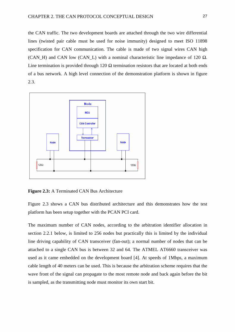
the CAN traffic. The two development boards are attached through the two wire differential
lines (twisted pair cable must be used for noise immunity) designed to meet ISO 11898
specification for CAN communication. The cable is made of two signal wires CAN high
(CAN_H) and CAN low (CAN_L) with a nominal characteristic line impedance of 120 Ω.
Line termination is provided through 120 Ω termination resistors that are located at both ends
of a bus network. A high level connection of the demonstration platform is shown in figure
2.3.
Figure 2.3: A Terminated CAN Bus Architecture
Figure 2.3 shows a CAN bus distributed architecture and this demonstrates how the test
platform has been setup together with the PCAN PCI card.
The maximum number of CAN nodes, according to the arbitration identifier allocation in
section 2.2.1 below, is limited to 256 nodes but practically this is limited by the individual
line driving capability of CAN transceiver (fan-out); a normal number of nodes that can be
attached to a single CAN bus is between 32 and 64. The ATMEL AT6660 transceiver was
used as it came embedded on the development board [4]. At speeds of 1Mbps, a maximum
cable length of 40 meters can be used. This is because the arbitration scheme requires that the
wave front of the signal can propagate to the most remote node and back again before the bit
is sampled, as the transmitting node must monitor its own start bit.

CHAPTER 2. THE CAN PROTOCOL CONCEPTUAL DESIGN
28
2.2 The Protocol Design Consideration
This section describes the development of the protocol from conception to implementation. It
describes how each of the supported message types is handled by the protocol and the
prioritisation of the message across the network. The priority of each of these supported
message types is determined by the CAN 29-bit identifier.
Every CAN message on the network contains a maximum of 8 bytes of data and this is a
limitation for large file transfers and thus large files are fragmented into small 8-byte packets
that can be transmitted on the CAN bus. CAN bus speed can go up to 1Mbps at 8MHz clock.
These bus considerations are critical to the detail design of the protocol. Another feature of
the CAN bus is a multi-cast and a multi-master architecture to provide system wide data
transfer consistency.
2.2.1 The CAN Identifier Assignment
The most important design requirement for a CAN protocol is the distribution of the identifier
information across the messages that will be handled on the CAN bus. The protocol is based
on CAN 2.0B and it uses the 29-bit ID to implement the supported message types. The
priority of the message on the bus is determined by the message ID and it is therefore
important to assign the identifiers during design time such that the messages intended as high
priority, for example the most time critical messages.
The 29 bit ID is divided into four fields as shown in figure 2.4 below.
Figure 2.4: A 29-Bit ID Allocation
Each of the above fields in the identifier has the following meaning based on the message
type it tags:
• Message type field - this field identifies what message type is sent on the network. There
are 32 possible different message types that can be addressed. Message type 0 is the highest
priority message.

CHAPTER 2. THE CAN PROTOCOL CONCEPTUAL DESIGN
29
• The file command, control, channel or index field - this is made specific by the type of
the message sent on the bus; in case of telemetry and telecommand messages this identifies
the channel and in case of the file or data transfer this field indicates the control or the
command field that specifies what must be done with the data that is read or written to a
specific memory address. This field will change to control flow index which monitors the
incoming data packets.
• The Source and Destination Address fields – each node will be allocated a unique
address to be used as the source during transmissions and as a destination address during
receptions. When a node gets a request it sets its acceptance filter with the destination address
field to its own node address and accept only frames addressed to it and on response the
source and destination fields are swapped and a response is sent.
The supported message types for this protocol are listed in table 2.3 below according to
priority from the lowest identifier value.
Time synchronization and debug messages will be broadcast messages as can be seen in table
2.3 below; their destination address is 0. Every node on the network must have their
acceptance filters masked to this broadcast address if they want to receive these messages.
These broadcast messages will not be acknowledged.
In all transmissions on the CAN bus all the addressing or message identification information
must be carried in the 29-bit arbitration field and the 8 byte data field must only be used for
data. All message types except for debug and the time synchronization messages will be
acknowledged and this acknowledgement will be a message type on its own as can be seen on
table 2.3. The xx symbols indicate an unassigned channel, source address or a destination
address and these are message packet dependant. The third column of table 2.3 gives a brief
idea of what each message type does.
Table 2.3: The Protocol Supported Message Types
Message Type Identifier Range Comment/Description
Time Synchronization 0x0000xx00 Broadcast Unix Time
Telecommand Request 0x01xxxxxx Command/Request

CHAPTER 2. THE CAN PROTOCOL CONCEPTUAL DESIGN
30
Telecommand Response 0x02xxxxxx Acknowledgement
Telecommand Not
Acknowledgement
0x03xxxxxx Command failure Reason
Telemetry Request 0x04xxxxxx Request
Telemetry Response 0x05xxxxxx Response
Telemetry Not Acknowledgement 0x06xxxxxx Reason
Unsolicited Telemetry Request 0x07xxxxxx Request for periodic response
File Header Transfer 0x08xxxxxx Start File transfer
File Header Transfer
Acknowledgement
0x09xxxxxx Response to initiate file
transfer
File Data Transfer 0x0Axxxxxx Data packets
File Data Transfer
Acknowledgement
0x0Bxxxxxx Each data packet
acknowledged
File Data Transfer Not
Acknowledgement
0x0Cxxxxxx Data packet lost
Debug Messages 0x0D00xx00 Broadcast string
2.2.2 Message Handling and Prioritization
Each of the message types in table 2.3 are designed to be handled in a specific way and a
description of each is detailed in this section. A brief reasoning as to why each message type
takes a specific priority will also be discussed as each message type is described.
• Time Synchronization - For the mission life of the satellite the CAN system needs to
communicate accurate and stable system time for all nodes to synchronize their UNIX time to
a master clock. Time synchronization should be done at regular intervals to keep all

CHAPTER 2. THE CAN PROTOCOL CONCEPTUAL DESIGN
31
subsystem events within real time limits and the whole system on time and accurate. This
would avoid using delayed or old data and to execute tasks synchronized with the data
measurements.
The master clock on the OBC or the GPS will broadcast the system UNIX time at regular
intervals. The time will be 6 bytes where the first 4 bytes will determine the time in UNIX
seconds and the next 2 bytes the second fraction in milliseconds. Time synchronization
messages have the highest priority on the bus because time accuracy is an important
parameter for the satellite applications like the attitude determination and control system
(ADCS).
The system time will be incremented every 1 millisecond and it can run from a timer interrupt
of a real-time clock on the OBC.
• Telecommand messages – In all cases these messages must be less or equal to 8 bytes in
the data field and no data fragmentation is required. Each message will be acknowledged
positively or negatively. There are 256 possible telecommand channels and only 15 standard
telecommand channels are currently reserved for the node and the application program can
expand the list to include user specific telecommand channels.
Table 2.4: Standard Telecommand Channels
TC Channel Number TC Description Approximate size Units
0x00 Clear the Run Time 0 bytes seconds
0x01 Clear CAN counters 0 bytes -
0x02 Clear Reset Counters 0 bytes -
0x03 Execute code at address 2 or 4 bytes Address
These messages are the second highest priority as can be seen on table 2.3. Table 2.4 lists the
standard telecommand channels. These are the standard channels implemented in the protocol
so far.
If a telecommand request has not been responded to after a specific period, the request for the
same channel can be made if the source of the request decides to do so.

CHAPTER 2. THE CAN PROTOCOL CONCEPTUAL DESIGN
32
A typical telecommand sequence exchange will look like figure 2.5 below. The acknowledge
message will be carrying the previous value of the specific channel or just an
acknowledgement saying a command has been executed or a not acknowledge message
specifying the reason.
Figure 2.5: A Telecommand Exchange
• Telemetry messages – they would be handled the same as the telecommand messages
above. The difference is on the data field; while the telecommand sends the command data the
telemetry message will contain no data and it requests data from the destination node. There
will also be 256 possible telemetry channels with 15 of those being the standard telemetry
channels. Table 2.5 lists these standard telemetry channels.
• Unsolicited Telemetry – the difference from normal telemetry messages is that
unsolicited telemetry responds periodically for each request. To setup an unsolicited telemetry
request, the repeat value and the repeat period must be specified. The repeat period will take 4
bytes of the 8- bytes data field and a further 2 bytes will determine the repeat value. If there is
a need to cancel an unsolicited telemetry; a request with the same channel and source address
must be made with a period of 0 or a repeat value of 0. To setup a request that repeats
indefinitely a repeat value of 0xFFFF must be specified. An Unsolicited telemetry request will
be setup as shown in figure 2. 6.

CHAPTER 2. THE CAN PROTOCOL CONCEPTUAL DESIGN
33
Repeat Period in seconds units Repeat Value
Data[0] Data[1] Data[2] Data[3] Data[4] Data[5]
Figure 2.6: Unsolicited Telemetry Format
Note: In future the resolution of the repeat period can be increased into a millisecond unit
resolution but care must be taken in specifying the repeat period because the 32 bit variable
representing milliseconds will overflow after approximately: (232/(1000))/(86400) ~ 49.71
days. So a repeat period of more 50 days cannot be specified and any period specified close to
overflow would lose that unsolicited telemetry request.
Table 2.5: Standard Telemetry Channels
Channel Number Telemetry Info/Data Approximate Size Units
0x00 Local Clock UNIX Time 6 bytes Seconds + milliseconds
0x01 Run Time 4 bytes seconds
0x02 Temperature 2 bytes 10th of ºC
0x03 CAN node Voltage(5V) 2 bytes 100mV
0x04 CAN node Current 2 bytes mA
0x05 TLM Requests 2 bytes -
0x06 TLM Response (Ack) 2 bytes -
0x07 TLM Response (Nack) 2 bytes -
0x08 TLCMD Requests 2 bytes -
0x09 TLCMD Response (Ack) 2 bytes -
0x0A TLCMD Response /Nack 2 bytes -
0x0B Reset Count 2 bytes -

CHAPTER 2. THE CAN PROTOCOL CONCEPTUAL DESIGN
34
0x0C Frames received 4 bytes -
0x0D Frames transmitted 4 bytes -
0x0E CAN Buss Off Count 2 bytes -
0x0F CAN Errors 2 bytes -
• File and data transfers – CAN has a small data payload per packet (8 bytes maximum)
which minimizes the bus throughput. Large file transfers would then need to be fragmented
into less than or equal to 8 bytes packets. When a large file is transferred across the CAN bus
a file transfer header is first sent. The header would contain 4 bytes to specify the memory
start address and the other 4 bytes of the 8 bytes data field will determine the total data size of
the file to be transferred.
During the file header transfer, the second field (the control field) of the 29-bit arbitration
field will contain the command to specify what data action will follow after the header
transfer has been acknowledged by the receiver.
The data transfer will begin immediately after the header acknowledgement and only one
packet of data will be transferred, the transmitting node will then wait for the
acknowledgement of that packet. The control field in this case will contain the data index
which specifies the packet number being transferred and this index is monitored against the
acknowledge that comes back. If the acknowledged index is not the same as the sent index,
the packet will be retransmitted. A retransmit will also happen if no acknowledge is received
within a specified timeout period. A retransmit of the same packet will be tried for 3 times
after which the whole file is aborted and declared undeliverable. An index sequence count
mechanisms are implemented at the receiver and if the incoming index is out of sequence the
packet will be discarded and a not acknowledgement response will be sent. If the packet with
the same index number is delivered for 3 times the receiver will abort the whole file transfer
and declare it undeliverable.
A typical situation that happens during file transfer is demonstrated in figure 2.7. The
transmitter of the file would be throttled by the receiver, this means that the receiver can send
a message that the transmitter must stop sending even before the file data is completely
received and it can also ask it to continue after a while. This throttling process shown in figure

CHAPTER 2. THE CAN PROTOCOL CONCEPTUAL DESIGN
35
2.8 below will depend on the available internal SRAM in the receiving node and the FLASH
programming procedure for a specific microcontroller when FLASH programming applies
and it will also depend at why the receiver decides to stop receiving data (e.g. an error on the
file being delivered, the node wants to execute a different high priority task or it tries to abort
data transfer because it has detected that the transmitter is faulty). The AT90CAN128 has a
specific sequence programming the FLASH memory. The sequence is as follows:
1) Fill a temporary buffer
2) Perform a page erase
3) Perform a page write
The AT90CAN128 FLASH memory is organized in pages and each page is 256 bytes in size.
In case of FLASH programming the receiver will throttle the transmitter after every 256 bytes
and after these 256 bytes have been successfully programmed into FLASH memory, a
continue message will be sent for more data to be programmed into FLASH memory.
For this microcontroller, programming FLASH and reading from FLASH requires two special
assembler instructions, Store Program Memory (SPM) and Load Program Memory (LPM)
respectively. These instructions must reside inside the Bootloader section and the interrupt
vector table must reside in the Bootloader section as well. This disables the interrupts from
the application section. It is therefore recommended that caution be taken when programming
or reading from the FLASH for the AT90CAN128 microcontroller.
When the full data file has been transferred across, the transmitter will release the connection
as shown in figure 2.7 below. The receiver of the file will release the connection, reassemble
the whole file and ultimately act upon it based on the command that was received in the
header. The typical file commands are:
• Program the FLASH
• FLASH Erase
• Execute program
• File read

CHAPTER 2. THE CAN PROTOCOL CONCEPTUAL DESIGN
36
Figure 2.7: File Transfer Flow Diagram Example
Figure 2.8: Transmitter Data Throttling Mechanism

CHAPTER 2. THE CAN PROTOCOL CONCEPTUAL DESIGN
37
All file commands will be acknowledged either positively or negatively depending on
whether the file operation was successful or not.
• Debug Messages – these lowest priority messages will be broadcast by a node which
wants to send certain debug information on the bus to all the nodes. This debug data will be
less or equal to 8 bytes. The typical information in the debug message can be the node status,
a node warning or debug information after a certain operation and will be used by any
application. Typical debug information message may look like figure 2.9.
Message Type CHL/Control Source Address Destination Address Data
0x0D 0x00 0xXX 0x00 “String”
Figure 2.9: A typical Debug Message
The 0xXX symbol means any source node can send the debug information and XX is the
source address. The control or channel field is 0x00 because there is no specific channel
addressed. In fact this field can contain anything for broadcast messages but it should always
be 0 for future compatibility and protocol expansion. Just like the time synchronization this
message is a broadcast message and therefore it will not be acknowledged.
2.3 Timing Analysis
The message priority and arbitration mechanism implemented in the CAN protocol means it
is difficult to deterministically analyse message latencies on the CAN bus. However, we need
to know the timing requirements of the application by analyzing the timing behavior of each
message sent on the bus. To do this time analysis the following assumptions about the way
messages are sent on the bus are made [1]:
1) A given message m has a known message length
2) The identifiers of all messages are known
3) Once buffered, message m cannot take longer time than Jm to be queued for transmission
by the CAN controller.
From the above assumptions, it is possible to compute the worst case latency, Rm of each
message on the bus. The latency [1] is given by:

CHAPTER 2. THE CAN PROTOCOL CONCEPTUAL DESIGN
38
Rm = Jm + Cm (2.1)
Where Jm represents the period of time a message waits in a queue (queuing jitter) and this
depends on how fast the CAN controller services it’s transmit buffer. Cm is the worst case
time delay to physically transmit a message on the bus. This does not include delays because
of contention on the bus. If it is assumed that there are no other messages being transmitted on
the bus and that the time the CPU takes to service it’s transmit buffer is negligible compared
to the total physical bus transmit delay then equation 2.1 is simplified to:
Rm = Cm (2.2)
Therefore, for an extended CAN frame,
Rm = [stuff bits + total overhead + data bits] x Tbit
Rm = [(54+8bm)/5] + 67 + 8bm x Tbit (2.3)
Where bm is the message size in bytes which ranges from 0 to 8 bytes and Tbit is the bit time
on the bus. From equation (2.3) above and the maximum CAN bus speed of 1 Mbps at a
maximum data payload of 8 bytes we have the worst case message latency of 154 µs. This
time analysis is a benchmark calculation and it will be used extensively in Chapter 4 when the
time analyses are done on each message type and the evaluation of the software drivers
overhead.

Chapter 3
Detailed Design and Protocol Implementation
This chapter presents the detailed system software design and its implementation. This
includes the description of how the low level drivers are developed for interfacing with the
hardware. It also looks at the CAN communication protocol in general. Application software
used during the system testing, as presented in chapter four, was implemented to test and
evaluate the CAN protocol.
3.1 The software structure
The relation between the OSI/ISO layer model and the proposed CAN bus protocol is shown
in figure 3.1. The CAN controller implements the entire physical layer and the data link layer
functionalities in hardware. However the software driver that interfaces to these layers must
provide a known and stable state during initialization.
Figure 3.1: A CAN/OSI Reference model
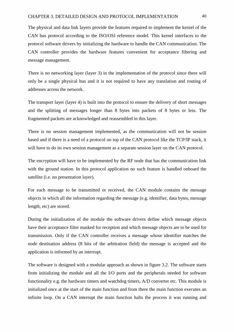
CHAPTER 3. DETAILED DESIGN AND PROTOCOL IMPLEMENTATION
40
The physical and data link layers provide the features required to implement the kernel of the
CAN bus protocol according to the ISO/OSI reference model. This kernel interfaces to the
protocol software drivers by initializing the hardware to handle the CAN communication. The
CAN controller provides the hardware features convenient for acceptance filtering and
message management.
There is no networking layer (layer 3) in the implementation of the protocol since there will
only be a single physical bus and it is not required to have any translation and routing of
addresses across the network.
The transport layer (layer 4) is built into the protocol to ensure the delivery of short messages
and the splitting of messages longer than 8 bytes into packets of 8 bytes or less. The
fragmented packets are acknowledged and reassembled in this layer.
There is no session management implemented, as the communication will not be session
based and if there is a need of a protocol on top of the CAN protocol like the TCP/IP stack, it
will have to do its own session management as a separate session layer on the CAN protocol.
The encryption will have to be implemented by the RF node that has the communication link
with the ground station. In this protocol application no such feature is handled onboard the
satellite (i.e. no presentation layer).
For each message to be transmitted or received, the CAN module contains the message
objects in which all the information regarding the message (e.g. identifier, data bytes, message
length, etc) are stored.
During the initialization of the module the software drivers define which message objects
have their acceptance filter masked for reception and which message objects are to be used for
transmission. Only if the CAN controller receives a message whose identifier matches the
node destination address (8 bits of the arbitration field) the message is accepted and the
application is informed by an interrupt.
The software is designed with a modular approach as shown in figure 3.2. The software starts
from initializing the module and all the I/O ports and the peripherals needed for software
functionality e.g. the hardware timers and watchdog timers, A/D converter etc. This module is
initialized once at the start of the main function and from there the main function executes an
infinite loop. On a CAN interrupt the main function halts the process it was running and

CHAPTER 3. DETAILED DESIGN AND PROTOCOL IMPLEMENTATION
41
executes the interrupt and once the interrupt is serviced the flow control goes back to the main
function and it resumes the task it was executing before interruption.
Figure 3.2: Protocol Software Modules
The main function calls the CAN receive handling function (CanRx ()) if there is a message
object that has received a valid message and this is done through polling the global receive
flag in the main function. This flag will be polled until all the message objects have been
serviced. To service a specific message object a corresponding call back function is
implemented in the CAN receive handling routine. If the routine that services a specific
message type is finished it returns to the receive routine and this routine will return to the
main function as shown in figure 3.2.
Figure 3.3: Protocol Software Structure

CHAPTER 3. DETAILED DESIGN AND PROTOCOL IMPLEMENTATION
42
The software drivers are developed to sit on top of the physical and data link layers. The
block diagram in figure 3.3 shows the software structure from the low level device drivers to
the application interface.
3.1.1 CAN interrupt Handling
The CAN controller interrupt for the AT90CAN128 originates from one of the sources as
shown in the interrupt structure in figure 3.4 below. The different interrupts that are enabled
and handled for this protocol are the following:
• Interrupt on receive complete OK
• Interrupt on transmit complete OK
• Interrupt on error (bit error, stuff error, crc error, form error, acknowledge error)
• Interrupt on “Bus Off”
There are other interrupts as shown in figure 3.4, but only the necessary interrupts were
enabled for the protocol development. The interrupt structure in figure 3.4 informs the
application of any communication that happens on the CAN bus. These interrupts are handled
by the implemented interrupt handling routine as shown in figure 3.5.
In figure 3.4 below CANSTMOB is the register which gives the status of each message object
and this register informs the application through an interrupt. The CANSTMOB is an 8-bit
register whose interrupt is enabled by activating the specific bits in the CAN general interrupt
enable register (CANGIE) , for example enable transmission interrupt bit indicated by ENTX
in figure 3.4.
When an interrupt occurs the corresponding bit is set in the CANSIT or CANGIT registers.
CANSIT register indicates the CAN status interrupt for a specific message object. CANGIT
register is the general interrupt register which gives the general interrupt status of the CAN
bus and not the interrupt status of a specific message object.
To acknowledge a message object interrupt, the corresponding bits of CANSTMOB register
(TXOK, RXOK etc) must be cleared by the software application and similarly for the general
interrupt bits.

CHAPTER 3. DETAILED DESIGN AND PROTOCOL IMPLEMENTATION
43
Figure 3.4: CAN Interrupt Structure
If a message has been received causing an interrupt, a receive flag is raised inside the interrupt
handling routine and the message interrupt flag must be cleared before returning to the main
function.
If the interrupt flag has not been cleared, the processor will generate the interrupt again once
the interrupt routine is exit. If the processor repeats this for a long duration the software will
hang and the watchdog timer will timeout and reset the node. This is avoided in the software
as shown in figure 3.5 by handling all possible CAN interrupts and by only enabling the
required interrupts used by the protocol during node initialization.
The receive flag is a global variable which will be polled in the main function to determine
and service the message object that caused the interrupt. The message object is not serviced
inside the interrupt handling routine, because the interrupt handling routine must execute as
fast as possible to make sure that no messages are lost due to long duration functions and
large code executed inside an interrupt handling function.
If the main function has serviced the receive flag it will clear this flag and then check if there
are any pending message objects that still need to be serviced. The CAN interrupt structure in
figure 3.4 is presented as a flow diagram as shown in figure 3.5 below. Only the transmit OK,

CHAPTER 3. DETAILED DESIGN AND PROTOCOL IMPLEMENTATION
44
receive OK, “Bus Off” and CAN error interrupts are enabled and handled by the interrupt
handling routine. The other interrupts will remain disabled since they are not used for the
protocol.
Figure 3.5: CAN Interrupt Flow Diagram
The flow diagram in figure 3.5 is entered if there is an enabled CAN interrupt and once
entered it checks the interrupt source and the interrupt is handled accordingly.
3.1.2 Node Initialization and configuration
In the AVR AT90CAN128 CAN controller there are 15 message objects in total. Each
message object is handled using the CANPAGE register as a pointer to select one of the 15
message objects. The message objects are stored as pages and the 15 message objects have the
same layout or format and they all have the same set of registers used to access the message
object properties that contain all the information about the message on the CAN bus ( e.g.
identifier, data bytes, message length, etc).
The message object registers have no initial (default) state and proper initialization is required
to make sure the node starts with a known state and the transmit message objects transmit as
required and the acceptance filters are setup to receive as required. The acceptance filter is a
CAN hardware mechanism that relieves the CPU from having to handle each and every

CHAPTER 3. DETAILED DESIGN AND PROTOCOL IMPLEMENTATION
45
incoming received CAN message. This allows the CPU to only respond to CAN frames it is
expecting (i.e. matches the message object acceptance filter). To setup the acceptance filter a
29-bit identifier mask is setup to enable the bits of the 29-bit identifier that must be checked
to enable reception. In this protocol the receiving node sets up the identifier mask to match its
8-bit node address in the destination address field. If the destination address matches, the
lowest message object number will accept the highest priority message based on the identifier
value of the incoming message. This message object will store all its values until a new
initialization is done and a transmission or reception is completed by that message object.
In this protocol implementation, 11 of the 15 message objects are enabled for reception and 4
are enabled for transmission. The message objects are reinitialized after use so that there is
always an available message object for transmission or reception. The other nodes in the CAN
network can have up to 32 message objects and how these are divided between being in a
transmit mode or receive mode will depend on the application. One of the 11 message objects
is enabled for broadcast and the broadcast address is 0, so every node will have their
acceptance filter setup to receive the message identifier with the destination address of 0.
As part of initializing the system designer is required to setup all the CAN nodes on the
network to the same baud rate. The maximum baud rate that can be setup on the CAN
network is 1 Mbps. The Bosch CAN specification allows the oscillator tolerance of 0.5 % at
1Mbps. For the AT90CAN128, the maximum oscillator frequency is 16 MHz and to achieve
baud rates up to 1Mbps a minimum clock frequency of 8 MHz must be setup in order to
comply with the CAN specification (i.e. one bit time must be between 8 and 25 time quanta
[1/clock frequency]).
3.1.3 System Control and Reset
The system software is developed to prevent the possibility for infinite loops causing the
software to hang and to eliminate any bugs that will prevent reliable network communication.
To ensure that the system recovers even in a rare case where the system hangs due to a
software bug, a watchdog timer is implemented to reset the system if such software
malfunctioning happens.
The watchdog timer times out every 2.2 seconds and it is reset at the beginning of the infinite
loop in main function. This watchdog timeout period is determined from the total time it takes
to execute the longest time consuming task possible on the network node. According to the
overall system design, one second sample period for the attitude determination and control

CHAPTER 3. DETAILED DESIGN AND PROTOCOL IMPLEMENTATION
46
(ADCS) system should be allowed for. It was decided that the watchdog timeout period
should at least be twice this worst case processing period to give a safety margin and
sufficient processing time for the other tasks.
In the AT90CAN128 microcontroller the watchdog timer is clocked from a separate on-chip
oscillator which runs at 1 MHz. In setting up the timeout period of 2.2 seconds this 1MHz
clock is divided by the watchdog prescaler.
Besides this watchdog reset each node can be reset if there is a new code upload. Upon node
bootup, the Bootloader will evaluate the reset source. If the reset is from the code upload
command then the boot-loader will jump to the new application code otherwise the boot-
loader will jump to the normal reset vector which will jump to the default current application
as shown in figure 3.6. All these Bootloader utilities and functionalities are to be implemented
on the boot-loader section as shown in figure 3.6.
3.1.4 System Timing
The system time is generated from a timer interrupt which increments the system time every
one millisecond. The GPS or the OBC master clock will broadcast the system UNIX time
every second. All the nodes will synchronize their time to this UNIX time and this time will
be 6 bytes in length (4 bytes time in seconds and 2 bytes of time in milliseconds). The
receiving nodes do not acknowledge this message. Each node will also be generating its own
local time from a timer interrupt and this local time is used by local tasks for time-outs or to
meet dead lines e.g. the unsolicited telemetry messages that will be scheduled on fixed
periods.
In setting up the 1 millisecond timer interrupt for the AT90CAN128 chip, Timer0 is used with
a timer prescaler factor of 64. The timer prescaler factor of 64 means that we divide the
system clock (the timer is clocked from 8 MHz system clock) by 64 to have a slower timer
increment. The 64 prescaler factor was chosen because it divides the 8 MHz clock into an
integer value that is a small enough for the timer registers, while small prescaler factors (i.e. 8
and 1) give too fast clock frequencies they need multiplication factors larger than 255. The
maximum reload value of 255 is possible with an 8-bit timer register. A prescaler larger than
64 (i.e. 256, 1024) need the floating point multiplication factors, that are not available in this
8-bit microcontroller, to be loaded on the timer registers. The 64 prescaler gives a time period
of 125 kHz and the timer will increment by 1/125 kHz = 8 microseconds and when we
multiply this by 125 we get the intended 1 millisecond time interval. Since Timer0 is an 8 bit

CHAPTER 3. DETAILED DESIGN AND PROTOCOL IMPLEMENTATION
47
timer or counter, we have to start the timer at 255 - 125 = 130 instead of 0 and count to 255.
This means that we get the timer ticks every 125* 8µs = 1.0000 milliseconds. The timer
register gets reloaded automatically every 1 millisecond on the timer overflow interrupt for
accurate time keeping. The 1 millisecond timer interrupt increments the local node system
time in milliseconds and seconds. However, the local node time gets synchronized both in
seconds and milliseconds to a periodical time synchronization message received as a
broadcast message.
3.2 Subsystem Level Message Handling
Every message that is transmitted or received on the CAN bus generates an interrupt in the
CAN controller and the application is informed by this interrupt as explained in section 3.1.1.
In the case of transmission the use of an interrupt structure is not necessary because the
transmission is initiated locally. The interrupt structure is affected in a sense that a transmit
flag will be raised when the message is transmitted and this flag needs to be cleared otherwise
the software will indefinitely stay in the interrupt handling subroutine.
In the case of message reception, an error or a bus-off interrupt flag, the interrupt handling
subroutine will handle each of these messages accordingly. If a message is received without
an error, the 16-bit receive status variable flag will be raised and the interrupt will return the
control to the main function loop. In the main function loop the received flag variable will be
polled as fast as the main function can execute. Each message received will set a bit in the 16-
bit status receive flag variable and a set bit will indicate the message object number that
caused the receive interrupt.
The main function will call the received message handling subroutine, passing the message
object number as a parameter. The received message handling routine extracts the message
from the message object and makes the message object available for a new transmission or
reception. The routine determines the message properties like the message length, the
message type, the source of the message and possibly the channel. The possible message
types that can be received are those tabled in table 2.3. The message handling routine
implements the callback function to handle each received message type. Each message type is
handled at a subsystem level as described in the following subsections.
3.2.1 Subsystem Telemetry Acquisition
In setting up a telemetry request, a message type specified by the 5 most significant bits of the
29-bit arbitration field. This 5-bit field is followed by an 8-bit channel which specifies which

CHAPTER 3. DETAILED DESIGN AND PROTOCOL IMPLEMENTATION
48
of the possible 256 channels is requested. The requesting node or subsystem will identify
itself in the next 8 bits of the 29-bit arbitration field as the source address; the requesting node
also specifies the destination address in the 8 least significant bits of the 29-bit arbitration
field.
Each local node will implement a set of standard telemetry channels and for this protocol 15
standard channels were implemented and these are tabled in table 2.5. A telemetry channel
number greater than the implemented channels would be a user application channel number
and a user telemetry subroutine handles these requests similar to the standard telemetry
channels. A channel larger than the maximum user channel number would be invalid and a
not acknowledgement message will be a response to such a message. If there is any data in the
data field during a telemetry request nothing will be done with the data because a telemetry
request normally contains no data in the data field.
In the AT90CAN128 node, the voltage channel was implemented using the voltage reader
supplied by the DVK90CAN128 development board. The input voltage is sampled by the
A/D converter. The voltage values are presented in 100mV units.
The temperature telemetry channel was measured from the DVK90CAN128 development
board temperature sensor that has a themistor with a negative temperature coefficient (NTC).
The voltages measured over the NTC are found using the A/D converter. These measured
voltages are used to calculate the themistor resistance (RT). Each themistor resistance
corresponds to a temperature value according to equation 3.1.
T = ß / ln (RT/R0) + ß /T0 (3.1)
Where, RT = Themistor resistance (Ω) at temperature T (°Kelvin) ß = Themistor beta-value (4250±3%) R0 = Room temperature themistor resistance (100 kΩ±5% at 25 °C) T0 = Room temperature (298 °Kelvin)
A temperature look up table based on equation 3.1 was implemented in software for
temperatures from -40 °C to +65 °C. Temperature values (1 °C steps) were used to compute
themistor resistance values. A table of the computed themistor values was stored in memory
as a look up table for corresponding temperatures. Only positive temperatures were observed
since the development environment was always indoors. Other standard telemetry channels
are implemented using the counters that increment or decrement at the change of state of each
channel.

CHAPTER 3. DETAILED DESIGN AND PROTOCOL IMPLEMENTATION
49
The message handling mechanism for normal telemetry messages apply to unsolicited
telemetry messages. In the case of unsolicited telemetry, the request will specify the repeat
period and the repeat count as explained in chapter 2. If the request is invalid, e.g. message
length not equal to 6 bytes or an invalid channel specified, the message reply will be a not-
acknowledge response. Specifying a repeat period of 0 seconds or a repeat value of 0 will
abort the ongoing unsolicited telemetry request. The inherent feature about aborting the
ongoing unsolicited or periodic telemetry request is that only the node that initially made a
request can abort that request. A maximum of 32 periodic unsolicited telemetry requests can
be handled simultaneously; once the periodic request has reached its repeat value it will
automatically clear the slot and make it available. If there are 32 periodic requests running
simultaneously, then another request will not be allowed and a ‘no slot available’ response
will be sent. The node that made a request must try again later once a slot becomes available
again. Although unlikely for this to happen, it is recommended that polling strategy be applied
by trying every minute until a slot is found.
3.2.2 Subsystem Telecommand Handling
The telecommand messages are high priority short messages and therefore are assigned
identifier values which gives them high priority on the bus.
Each node that requires a specific remote task to be performed would send a command on the
CAN bus and it must specify the destination node and the addressed channel. A telecommand
request contains a command of not more than 8 bytes in the data field. There are 256
addressable telecommand channels and only a few were implemented for this protocol as a
means to demonstrate the handling of telecommand messages. The implemented standard
telecommand messages are presented in table 2.4. In a similar manner to the standard
telemetry channels, 15 of the possible 256 are reserved for commanding the local node to do
basic telecommand messages e.g. clearing the node CAN error and message counters. If the
addressed telecommand channel number is above 15 it will be handled by the user
telecommand subroutine and if it is above the maximum user channel number it is an invalid
channel.
On reception of a valid telecommand request the node will perform the required action and
send an acknowledgement indicating that the task has been performed. Depending on the
telecommand requested, the telecommand response or acknowledgement may be used to send
telemetry data corresponding to the channel addressed. For example, if the telecommand is to
clear the CAN error and message counters as part of the acknowledgement, the current

CHAPTER 3. DETAILED DESIGN AND PROTOCOL IMPLEMENTATION
50
counter values may be sent. This is possible because the telecommand acknowledgement is a
message type on its own and if this message type is received it means a requested command
has been performed and we can use the data field for telemetry data. It has to be noted that a
maximum of 8 bytes can be sent in a telecommand acknowledge message.
If a telecommand message is unrecognized or invalid, a telecommand not-acknowledge
message will be a response to this message. The response in the data field will specify the
reason why the telecommand was not performed or why it was invalid e.g. the addressed node
is not allowed to execute the command, the channel is above maximum the user channel or
the specified value is out of the range.
In demonstrating telecommand handling, one AVR node was used to command another AVR
node to clear the counters listed in table 2.4.
3.2.3 Data Transfers
In starting a transmission of a large file, a file header is sent which specifies a 4-byte start
address and a 4-byte data size. If the start address specified tries to access a prohibited
memory or when the specified data length is longer than the available memory, the
application must respond with a not-acknowledge response.
The header must be acknowledged positively within a 1 second timeout period before the data
transfer begins. If the header has not been acknowledged the transmitter will retry this process
for 3 times, after which it stops and broadcasts an error message on the bus that the message is
undeliverable.
The transmission of messages larger than 8 bytes on the CAN bus requires the fragmentation
of the message into packets of 8 bytes or less. Once a fragmented packet is sent on the bus,
the transmitter waits for the acknowledgement before the next packet is sent and this process
is done until the whole data file is sent over. A timeout mechanism is implemented to provide
for a robust transmission of the data. After each data packet is transmitted, an
acknowledgement must be received before a timeout period of 1 second elapses. If no
corresponding acknowledgement is received within this timeout period a retransmit is done
and this is retried 3 times after which the file is declared undeliverable. As explained in
section 2.2.2 the transmitter will be throttled, meaning that the receiver can reply with
message to the transmitter telling it to stop sending more data. The receiver will then send
another message when it is ready to receive more from the source of the file data, the
communication process will then resume again.

CHAPTER 3. DETAILED DESIGN AND PROTOCOL IMPLEMENTATION
51
The file transfer is delivered as shown graphically in figure 2.7 and once the complete file has
been delivered it will be assembled by the receiver node. The command that was received in
header will now be executed (e.g. write the data into the FLASH, update the calibration tables
in the SRAM, or read data from the FLASH and transfer it to the serial modem link to the
ground station). This is done on the transport layer of the OSI reference layer as shown in
figure 3.1.
The most important large file operations handled by the protocol are the following:
• Code Upload & Execution
In programming new application code to the FLASH, the AT90CAN128 follows a special
sequence and the data is buffered in a page by page fashion (a page is 256 bytes). This is a
classic case where a node during code upload can throttle the transmitting node after a page
buffer has been filled. The data is delivered by the CAN interface and it is first dumped in the
SRAM of the receiving node as shown if figure 3.6 below. When the page buffer size data is
sent the receiving node will send a successful data reception acknowledge with a ‘stop
sending message’. The sequence that this chip follows to program the FLASH is as follows
and this is shown in figure 3.6:
1) Fill the temporary buffer (256 bytes)
2) Perform a page erase
3) Perform a page write
During the FLASH programming sequence the interrupt vectors and the CAN communication
routines must reside on the boot section. The CAN interrupts and routines will be disabled in
running application and a copy of the CAN application code must run in the Bootloader
section. Furthermore, the special Bootloader utilities (e.g. the interrupt vectors and CAN
service routines, reset vectors, special FLASH programming utility routines [program
FLASH, erase FLASH memory, read from FLASH memory and execute program memory]
etc.) must reside in the boot section to facilitate the FLASH programming and to enable the
start of the new application.

CHAPTER 3. DETAILED DESIGN AND PROTOCOL IMPLEMENTATION
52
Figure 3.6: Code Upload Diagram
The data is transferred from the SRAM into the temporary buffer in the FLASH memory and
this temporary storage provides non-volatile storage before a page erase at a desired address is
performed.
The reason why data is first dumped into the temporary buffer is because a FLASH erase
operation must be done before writing to a FLASH address.
If there is any reset or power down during page erase at a specified address, the code segment
that has been buffered will still be available. This will avoid the corruption of the stable
running application unless a new code segment is buffered in non-volatile memory. If the
reset or power down happens during the SRAM to temporary buffer transfer happens, then it
will not present a problem because nothing is yet erased or corrupted in the old application
code segment.
Dummy functions for the programming sequence mentioned above have been provided for in
the protocol implementation and the future application developer must develop these
functions together with the Bootloader software.
Once the complete file is written in FLASH memory the boot software will jump to the new
application on a ‘code execute’ command from a specific address, otherwise the code that is
in the Bootloader section will stay executing. It is recommended that once the new code has
been uploaded or a specific part of the code in FLASH is updated, the new application can be
started.

CHAPTER 3. DETAILED DESIGN AND PROTOCOL IMPLEMENTATION
53
Figure 3.7: Code Segment Update and Code Upload
Two common update procedure flow charts are shown in figures 3.7. Figure 3.7a describes
updates for small parts of FLASH e.g. a constant table stored in FLASH memory. Figure 3.7b
shows a large code upload at a specified address and data length.
• Reading Data from Memory
On reception of a ‘read request header’ command, the local node will evaluate the start
address and the length to see if the request tries to access a valid memory address. If a request
tries to read from an invalid or a prohibited address, the application program will send a ‘not
acknowledge’ response, specifying that a wrong address is being accessed. If the request is
valid, the local node acknowledges the header and initialize the file transfer as if data transfer
request was done locally (i.e. it will send the header message and wait for an
acknowledgement). It will then start to transfer the data from the requested address. While
receiving the data, the process can get aborted or throttled by the node that requested the data.
The node being ‘read requested’ will not specify a start address for the data requested, but it

CHAPTER 3. DETAILED DESIGN AND PROTOCOL IMPLEMENTATION
54
will specify the data length. The node that requested the data will store the data in its own
predetermined memory address.
Reading from the FLASH memory would most probably be for the reason that is illustrated in
figure 3.7a above. This figure shows a small piece of code to be updated, e.g. a parameter
table being read from the FLASH to modify and then by writing it back to the FLASH.
The temporary buffer is not necessary when reading from the FLASH and the code is read
directly form the FLASH memory to the SRAM.
It must be noted that the work on the boot software application is in development in this
protocol and must be further refined to interface with the data transfers as explained above.
Reporting on the data transfer mechanisms is done here, because extensive work was already
done on this, but could not be implemented as the boot software was not completely
developed due to time constraints. Once the boot software is developed, then the data can be
programmed into the FLASH. The programming of the FLASH needs subroutines to erase
and program the FLASH. The code must reside in the Bootloader section, especially the code
using the SPM and LPM instructions for the AT90CAN128 microcontroller.
In testing the large data file transfers in the protocol, large blocks (e.g. 2 kbytes) of data were
transferred into the SRAM from the source node. Dummy functions (nothing is done in these
functions, just a return to the caller) were implemented as boot software and the whole
process of file transfer was carried out as explained in this section.
3.2.4 Debug Messages
These low priority messages were implemented by broadcasting a text string on the CAN bus
and the nodes receiving this text string will store it on a local variable which could be read
and acted upon. These messages are not acknowledged and can be used by an application that
wants to report anything on the bus or warn other nodes about anything happening on the
CAN bus or to warn other nodes about errors or to broadcast a node’s status and health.

Chapter 4
Protocol Performance and Implementation Results
In evaluating the protocol performance, the software response time for each supported
message type was measured. The system was also stress-tested by continuously sending
messages one after another as fast as possible and observed when the system software started
to malfunction. The maximum practical bus speed was also observed as the messages were
sent from the minimum CAN bus speed (5kbps) to the maximum CAN bus speed (1Mbps)
but only selected bus speeds were tested as the PCAN PCI card provided discrete bus speeds
for monitoring and testing. Power consumption is also measured when there is
communication on the CAN bus as well as when CAN bus is idle.
4.1 Hardware Performance Measurements
As mentioned in the previous chapters, the protocol was demonstrated on two
DVK90CAN128 development boards and the measurements here include the other board
components. The two development boards were supplied from a 5V DC power supply. The
hardware system setup is shown in figure 4.1 below.
Figure 4.1: System Test Setup

CHAPTER 4. PROTOCOL PERFORMANCE AND IMPLEMENTATION RESULTS
56
The board current measured when there was no CAN communication on the bus was 42 mA.
When a 2-kilobytes file transfer was initiated on the CAN bus the current increased from
42mA to 43 mA and when the file transfer was completed the current just normalized back to
42mA. These were only possible current measurements regarding the CAN bus protocol and
the software drivers as this was a development board and no specific hardware components
were designed.
The expected AVR AT90CAN128 power consumption when the microcontroller is used in a
board designed for only CAN communication and Nanosatellite application should ideally be
close to the power characteristics shown on page 386 of the AT90CAN128 datasheet [4]. The
attractive power consumption for this microcontroller is when it is supplied from a 3.3V
supply and it draws 10mA at 8 MHz
The supply voltage was measured as well on the configuration pads supplied on the board to
compare it with the 5V from the power supply and the actually measured value was 5V ± 0.5
for a number of measurements taken. The voltage was also measured using the voltage
reading capability of the board. The voltage coming into the board was connected to one of
the inputs of the analog to digital converter and the output was measured and the
measurements were 5V ± 0.3 for a number of measurements that were taken. The voltage
reading capability was used to supply the voltage value as a telemetry data. The board had no
current sensor and thus no current telemetry data were measured.
4.2 Software Time Response
The time measurements were based on the maximum CAN bus speed of 1 Mbps. The latency
of each of the supported message types was measured when one specific message type was
sent on the bus. The timing analyses become complex when more than one message is sent
randomly on the CAN bus. The message priority and bus contention arbitration mechanisms
add to the complexity of timing analysis. The latencies measured the time it took from
sending a request to the time the total response is received and these are listed in table 4.1.
The message latencies were measured using one of the port pins in microcontroller. The pin
was pulled high when the transmission started and it was pulled low when the response was
completely received. The time duration with the pin high was measured for each of the
messages. However, for the broadcast messages, i.e. the time synchronization and debug
messages, where no response is received, the latency is measured as the time it took to write

CHAPTER 4. PROTOCOL PERFORMANCE AND IMPLEMENTATION RESULTS
57
the message into the transmit buffer until it has been transmitted. This time duration was
measured by pulling an I/O pin high when the transmit routine is entered and pulled low when
the transmit complete flag has been raised.
Table 4.1: Message Latencies Message Type Data Size Latency
Normal Telemetry 0 bytes request + 4 bytes response 900 µs
Unsolicited telemetry 6 bytes request + 6 bytes response 1.2 ms
Telecommand 4 bytes command + 8 bytes response 1100 µs
File Data Transfer 2 Kbyte (256 8-byte messages) + 256
bytes( 1 byte acknowledgements)
214 ms
Time synchronization 6 bytes 468 µs
Debug message 8 bytes 300 µs
The port pins were used, because the smallest time resolution the system time was setup for
was a millisecond from the timer interrupt routine. This meant that time measurements below
millisecond resolutions needed a software change in the timer interrupt routine that was used
for system time.
The results in table 4.1 show that the software overhead contributes significantly to the
message response latencies. For example the 2 Kbyte file transfer without any software
overhead should be transferred as follows:
Total bits = 8-Byte Header + 1-byte Header Ack +
256 (8-byte) data packets + 256(1-byte) data Ack’s (4.1)
The total bits sent for this 2 Kbyte file transfer including the protocol overhead (start bits +
CRC bits + arbitration bits + stuff bits etc) is:
Total Data in Bits = 154 + 98 + 154*256 + 98* 256 = 64764 bits (4.2)

CHAPTER 4. PROTOCOL PERFORMANCE AND IMPLEMENTATION RESULTS
58
For a maximum CAN bus speed (1 Mbps) this 2 Kbyte file transfer should take:
64764*1e-6 = 64.764 ms
This is just a theoretical value and it assumes that the data is transmitted continuously in
sequence without delay between CAN packets. This is an impractical approach on the CAN
network, because there has to be a software overhead which makes sure the data is stored at a
required location and be transferred in a correct sequence, thus the need to have the protocol.
Due to the CAN packet data field limit, to transfer a 2 Kbyte file on the CAN bus there has to
be a fragmentation of the file into 8-byte packets. This fragmentation mechanism will take its
time to fragment the file and send the correct fragments in sequence. The software also adds a
bit of overhead when it checks the index sequence at the receiver end before each packet is
acknowledged. At the transmitter the acknowledged index is also checked before the next
packet is sent. The propagation delays are also not included in the theoretical value above.
The message latency of 214 ms is therefore a realistic value given the software overhead to
implement the file transfer protocol explained above. The other message latencies are also
within acceptable real time response limits, for example sending a 6-byte time
synchronization message should theoretically take 138 µs but it takes 468 µs because of the
software overhead.
4.2.1 Main Loop Execution Time Response
All the application programming interface routines are handled by the main function using the
flags. The main function just initializes the software drivers and then enables the watchdog
timer at the start of the infinite loop as shown in figure 4.2.

CHAPTER 4. PROTOCOL PERFORMANCE AND IMPLEMENTATION RESULTS
59
Figure 4.2: Main Function Flow Diagram
The CPU will execute this main loop as fast as possible and the software was optimized such
that no messages would be lost as a result of a main loop that takes too long to service all the
service routines and to execute all required application tasks.
The main loop frequency was measured with the following events happening with all the
interrupts enabled (timer interrupt always incrementing the system time every millisecond):
1) Minimum execution time with no CAN activity on the bus (no messages to handle but
just checking flags and servicing interrupts).
2) Maximum execution time with a lot of CAN activity on the bus (most CAN supported
message types handled on the bus).
Table 4.2: Main Loop Execution Time
Main Loop Event Execution Time
Minimum execution time with no CAN
messages on the bus
370 ns (2.70MHz)
Maximum execution time for a lot of CAN
activity handled
19.00 µs
(52.63KHz)
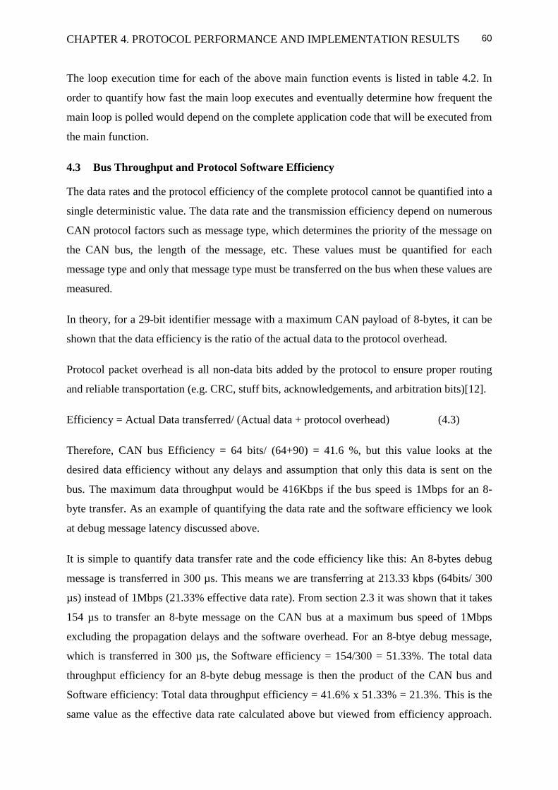
CHAPTER 4. PROTOCOL PERFORMANCE AND IMPLEMENTATION RESULTS
60
The loop execution time for each of the above main function events is listed in table 4.2. In
order to quantify how fast the main loop executes and eventually determine how frequent the
main loop is polled would depend on the complete application code that will be executed from
the main function.
4.3 Bus Throughput and Protocol Software Efficiency
The data rates and the protocol efficiency of the complete protocol cannot be quantified into a
single deterministic value. The data rate and the transmission efficiency depend on numerous
CAN protocol factors such as message type, which determines the priority of the message on
the CAN bus, the length of the message, etc. These values must be quantified for each
message type and only that message type must be transferred on the bus when these values are
measured.
In theory, for a 29-bit identifier message with a maximum CAN payload of 8-bytes, it can be
shown that the data efficiency is the ratio of the actual data to the protocol overhead.
Protocol packet overhead is all non-data bits added by the protocol to ensure proper routing
and reliable transportation (e.g. CRC, stuff bits, acknowledgements, and arbitration bits)[12].
Efficiency = Actual Data transferred/ (Actual data + protocol overhead) (4.3)
Therefore, CAN bus Efficiency = 64 bits/ (64+90) = 41.6 %, but this value looks at the
desired data efficiency without any delays and assumption that only this data is sent on the
bus. The maximum data throughput would be 416Kbps if the bus speed is 1Mbps for an 8-
byte transfer. As an example of quantifying the data rate and the software efficiency we look
at debug message latency discussed above.
It is simple to quantify data transfer rate and the code efficiency like this: An 8-bytes debug
message is transferred in 300 µs. This means we are transferring at 213.33 kbps (64bits/ 300
µs) instead of 1Mbps (21.33% effective data rate). From section 2.3 it was shown that it takes
154 µs to transfer an 8-byte message on the CAN bus at a maximum bus speed of 1Mbps
excluding the propagation delays and the software overhead. For an 8-btye debug message,
which is transferred in 300 µs, the Software efficiency = 154/300 = 51.33%. The total data
throughput efficiency for an 8-byte debug message is then the product of the CAN bus and
Software efficiency: Total data throughput efficiency = 41.6% x 51.33% = 21.3%. This is the
same value as the effective data rate calculated above but viewed from efficiency approach.

CHAPTER 4. PROTOCOL PERFORMANCE AND IMPLEMENTATION RESULTS
61
The efficiencies and data rates of the other message types can be calculated in the same way
as shown for the debug message above and these were calculated and listed in table 4.3
below.
Table 4.3: Throughputs and Efficiencies
Message Type Effective Data Rate
(kbps)
Protocol Software
Efficiency (%)
Total Data
Throughput (%)
Debug Message 213.33 51.33 21.35
Time Synch. 102.56 29.49 12.27
Telemetry 35.55 23.55 9.79
Unsolicited
Telemetry
80.00 23.00 9.57
File Data
Transfers
86.47 30.26 12.59
Telecommand 87.27 25.09 10.44
The general data throughput for different message lengths on the CAN bus is plotted for an
extended frame format and the standard frame format as shown in figure 4.3. These graphs are
plotted with the assumption that there is only one message on the CAN bus and there are no
priority and bus contention issues.
The implementation specific bus throughput graphs for different message types with different
message lengths can be computed like in table 4.3 and be compared to figure 4.3. Different
message types have different fixed message lengths depending on the application and to
compute data throughputs the length of a message must be known and the transfer speed be
measured. The throughput should be the same as in figure 4.3 besides that the transfer speed
would be reduced due to propagation delays and the software overhead as discussed above.

CHAPTER 4. PROTOCOL PERFORMANCE AND IMPLEMENTATION RESULTS
62
1 2 3 4 5 6 7 850
100
150
200
250
300
350
400
450
500
Data Length Code [bytes]
Max
imum
Net
Bus
Thr
ough
put
[K
bits
/sec
ond]
CAN Bus Throughput
Extended Frame Format(29-bit)
Standard Frame Format(11-bit)
Figure 4.3: CAN Bus Throughput
4.4 Software Reliability
In testing how reliable the software handled all possible CAN communication, a test was
done where multiple message types were sent on the CAN bus. A total of 8 unsolicited
telemetry requests were made from the PCAN PCI card to run simultaneously. The two
development boards kept requesting telemetry data from each other. One node was setup to
transfer 2 kilobytes of data while it also broadcasted time synchronization message. All the
communication described above continued for a long time and the performance was
consistent.
Different messages were also sent from the PCAN PCI card and the two boards just handled
them efficiently. The messages from the PCAN PCI card were sent using the spacebar on the
keyboard. When the spacebar was pressed indefinitely the messages were sent from the PCI
card as quick as the CAN controller embedded on the card could transmit the messages, and
the CAN software still preformed as expected and no messages were lost.
The software functionality was tested at most CAN bus speeds (5kbps to 1Mbps), especially
those that are provided by the PCAN PCI card, and it gave the expected performance. Testing

CHAPTER 4. PROTOCOL PERFORMANCE AND IMPLEMENTATION RESULTS
63
the bus performance at non-standard speeds, e.g. 570 kbps could be done but the tests that
were done at the standard CAN bus speeds (5kbps to 1Mbps) provided by the PCAN PCI card
for monitoring were enough tests for reliable handling of messages on the CAN bus. To
compute and setup the bit timings for testing at different baud rates the procedure provided in
Appendix B must be followed [8].

Chapter 5
Conclusion and Recommendations
The primary objective of this research project was to design a communication protocol that
will handle real time messages onboard a Nanosatellite. To achieve this, a survey was done on
various communication bus standards and high application layer protocols. The research was
driven by a number of factors specific for the Nanosatellite application and these include use
of low power components, cost, flexibility and reliability.
5.1 Conclusion
The communication protocol was designed to handle Nanosatellite messages on a CAN bus.
The design included specifying the types of messages the protocol would handle and the
implementation thereof. To implement an efficient and reliable communications protocol the
CAN bus protocol standard was chosen for the lower communication layers as motivated in
chapter one of this document. The CAN specification only provided for the low level
communication protocol (physical layer and the data link layer). This meant that the higher
application protocol needed to be designed on top of the CAN protocol specification to handle
a Nanosatellite application.
A survey was conducted on the higher application layer protocols including the previous
protocols developed in the ESL and the CAN based commercial protocols like CANopen and
DeviceNet. It was concluded that these commercial protocols would limit the flexibility and
the optimization of the Nanosatellite application since these protocols are optimized for
general use. The protocol was then developed from conception to the implementation with
consideration of specific Nanosatellite requirements.
A low cost test setup was chosen after a survey on microcontrollers supporting a CAN
interface. The test setup was chosen to be an AVR (AT90CA128) 8-bit CMOS
microcontroller which provided attractive features (e.g. power consumption of 33mW at 5V)
and it had a lot of software development support. Two identical AVR development boards
were used in the system setup and a PCAN PCI card was used to monitor the traffic on the
CAN bus. Messages like telemetry, telecommand, time synchronization, debug information

CHAPTER 5. CONCLUSION AND RECOMMENDATIONS
65
and large file transfers were specified as the main communication messages for the
Nanosatellite.
In order to manage the communication on the CAN bus, one of the design procedures was to
distribute CAN identifiers according to the priority of each message on the bus. Low level
hardware drivers, middleware software drivers and the application programs were developed
to evaluate the full protocol functionality.
The performance results of the developed protocol implementation were measured in terms of
software efficiency, bus throughput, software response latencies and software reliability under
extreme bus traffic conditions. All the messages were handled by the protocol as expected and
the performance measurements are presented in chapter four of this document.
The results can be summarized as follows:
• The software response times for each of the messages were within the real time limits.
Latencies were as expected greater than theoretically deterministic values because of the
software overhead.
• The bus throughputs and software efficiencies are within the acceptable limits. These
were further endorsed by the system that reliably handled all CAN traffic when left to run for
a long time.
• When large messages are transferred, acknowledging each and every packet reduced the
protocol efficiency drastically (e.g. file transfer bus throughputs of 12.59 %) but this
improved reliability, data consistency and reduced software complexity.
• The power consumption was 42 mA (at 5VDC) when there was no CAN
communication and it increased to 43mA when a CAN packet was sent. These power
measurements were done with extra development board components. More absolute CAN
communication power measurements can be done once a new node with only components
necessary for CAN communication has been designed.
The AVR microcontroller requires a certain procedure to be followed when programming
large files or when code uploads are needed to the FLASH memory. The procedure included
the requirement to develop Bootloader software and certain programming procedures to reside
inside the Bootloader section. The latter will facilitate the firmware updates or large file

CHAPTER 5. CONCLUSION AND RECOMMENDATIONS
66
transfers. The development of the Bootloader software also demanded an additional time
frame. It was decided that to demonstrate large file transfers, large data blocks will be
transferred from the SRAM of a source node to the SRAM of the destination node. Once the
Bootloader software has been developed a final step will be to program the data into FLASH
memory. The following subsection recommends how code updates and large file transfers
should be programmed to FLASH memory.
5.2 Recommendations
This section presents some suggestions for future work to further optimize the functionality of
the developed communications protocol.
As mentioned above, the software was completely developed on the AVR development
boards. It is recommended that a new hardware design be completed, based on an AVR
AT90CAN128 microcontroller to evaluate the protocol when only the necessary components
for the CAN communication are used. Another hardware consideration can be to develop the
protocol on a microcontroller that has a large SRAM and FLASH capacity, since the
AT90CAN128 chip provides only 4 kbytes of SRAM and 128 kbytes of FLASH. A memory
constraint was noted during protocol development as ultimately only 2 kbytes of data could be
used to test large file transfers because of the limited size of SRAM memory. An alternative
to the SRAM constraint would be to connect an external SRAM as suggested on the
AT90CAN128 data sheet.
When transferring large messages, Bootloader software must be programmed to transfer data
to the FLASH memory. Dummy subroutines were implemented in the software to show how
the Bootloader software should interface with the file transfer routines. Assembler low level
code is also presented in Appendix C for the subroutines that must be implemented in the
Bootloader for the AVR microcontroller. Other microcontrollers may have a different
mechanism of programming FLASH and therefore the sample code will not apply to them.
Another important future consideration will be to test the software when the number of
communication nodes increase from the current three nodes used during testing. This will
increase the CAN communication on a large network to evaluate the software reliability and
software response latencies under extreme communication load which could affect the real
time performance of the system.

CHAPTER 5. CONCLUSION AND RECOMMENDATIONS
67
The protocol was implemented on a single CAN bus physical layer and this means if the bus
fails then the whole system fails. It is therefore recommended that the redundant (backup)
physical bus be developed since the OBC already provides two CAN bus interfaces. However,
a protocol extension is required to accommodate the architectural changes as it will affect the
network management and routing of the data between the two bus networks.

Bibliography
[1] Lawrenz W., “CAN System Engineering: From Theory to Practical Applications”,
1997, Springer-Verlag, New York
[2] Koekemoer J.A., “Investigation of a Command and Data Handling Architecture for
SUNSAT-2 Micro Satellite”. Thesis presented in partial fulfillment of the requirements
for the degree-Masters of Science in Electronic Engineering at the University of
Stellebosch, 1999
[3] http://www.embedded.com/97/fe29709.htm.
[4] http://www.atmel.com
[5] http://www.peak-system .com
[6] http://www.hpinfotech.com
[7] CAN for space,
ftp://ftp.estec.esa.nl/pub/wsd/CAN/canspace.htm
[8] http://www.avrfreaks.net/index.php?module=FreaksArticles&func=viewArticles
[9] Tindell, K., Burns, A., “Guaranteeing Message Latencies on Controller Area
Network”. Proceedings of the First International CAN Conference, Germany,
September, 1994.
[10] Tindell, K., Burns, A., and Welling, A., “ Calculating Controller Area Network (CAN)
Message Response Times”, 1995
[11] CAN/Ethernet,
http://www.warwick.ac.uk/devicenet/downloads.htm
[12] Upender, B. and Koopman, P., "Embedded Communication Protocol Options,"
Proceedings of Embedded Systems Conference 1993, Santa Clara, pp. 469-480,
October, 1993
[13] Bosch, CAN Specification, Version 2.0, Robert Bosch GmbH, Stuttgart, 1991

BIBLIOGRAPHY
69
[14] Woodroffe A.M. and Madle P., “Application and experience of CAN as a low cost
OBDH bus system”, MAPLP 2004, Washington D.C. USA, September, 2004
[15] Farr X.C., “Development of A Fault-Tolerant Bus System Suitable for A High-
Performance Embedded Real-Time Application on SUNSAT’s ADCS” Thesis
presented in partial fulfillment of the requirements for the degree-Masters of Science
in Electronic Engineering at the University of Stellebosch, 2000
[16] Patrick, J., Serial Protocols Compared”, Embedded.com, 2002, http://www.embedded.com/9900637?_requestid=1098733
[17] IEG (Information and Electronics Group) at the Ohio State University, 2000, http://www.ece.osu.edu/ie/main/CurrentResearch/SPI_Nautilus_chip/
[18] Soffel, V., “Synchronous Microcontroller Communication Interfaces: SPI and Microwire versus I2C” , May, 2003
[19] Wertz, J.R. and Larson, W.J., “Space Mission Analysis and Design”, Third Edition,
Microcosm, 1999 [20] Profibus Technical Information,
http://www.samson.de/pdf_en/l453en.pdf
[21] Boterenbrood, H., “CANopen - high level protocol for CAN-bus”, Version 3.0, Amsterdam, March, 2000.
[22] CAN-in-Automation, CANopen, CAL-based Communication Profile for Industrial Systems, CiA DS-301, Version 4.0, June 16 1999. http://www.can-cia.org/
[23] Rinaldi, J., Wendorf, J. DeviceNet: A Plan for Product Developers, 2002
http://www.rtaautomation.com/devicenet/494ds/DeviceNet_in90Days.pdf [24] http://www.odva.org/

Appendix A
Controller Area Network - CAN Information
A.1 What is CAN?
Controller Area Network (CAN) is a serial network that was originally designed for the
automotive industry, but has also become a popular bus in industrial automation as well as
other applications. The CAN bus is primarily used in embedded systems, and as its name
implies, is the network established among microcontrollers. It is a two-wire, half duplex,
high-speed network system and is well suited for high speed applications using short
messages. Its robustness, reliability and the large support from the semiconductor industry are
some of the benefits with CAN.
CAN theoretically addresses up to 2032 (CAN standard frame format) or more than 5 million
(CAN extended frame format) devices (assuming one node with one identifier) on a single
network. However, due to the practical limitation of the hardware (transceivers), the number
of nodes per network is determined by the transceiver fan-out. It offers high-speed
communication; up to 1 Mbits/s thus allows real-time control. In addition, the error
confinement and the error detection capability makes it more reliable in noise critical
environment.
A.2 CAN standards
The original specification is the Bosch specification. Version 2.0 of this specification is
divided into two parts:
• Standard CAN (Version 2.0A). Uses 11 bit identifiers.
• Extended CAN (Version 2.0B). Uses 29 bit identifiers.
The two parts define different formats of the message frame, with the main difference being
the identifier length.

APPENDIX A. CONTROLLER AREA NETWORK – INFORMATION
ii
There are two ISO standards for CAN. The difference is in the physical layer, where ISO
11898 handles high speed applications up to 1Mbit/second. ISO 11519 has an upper limit of
125kbit/second.
A.3 How CAN works?
Introduction
As stated earlier, CAN is a multimaster network. It uses CSMA/CD+AMP (Carrier Sense
Multiple Access/Collision Detection with Arbitration on Message Priority). Before sending a
message the CAN node checks if the bus is busy. It also uses collision detection. In these
ways it is similar to Ethernet. However, when an Ethernet network detects collision both
sending nodes stop transmitting. They then wait a random time before trying to send again.
This makes Ethernet networks very sensitive to high bus loads. The CAN protocol solves this
problem with the principle of bit wise arbitration.
A.3.1 Principle
Data messages transmitted from any node on a CAN bus do not contain addresses of either
the transmitting node or of any intended receiving node.
Instead, the content of the message is labelled by an identifier that is unique throughout the
network. All other nodes on the network receive the message and each performs an
acceptance test on the identifier to determine if the message, and thus its content, is relevant
to that particular node.
If the message is relevant, it will be processed; otherwise it is ignored.
A.3.2 Identifiers and arbitration
The unique identifier also determines the priority of the message. The lower the numerical
value of the identifier, the higher the priority. This allows arbitration if two (or more) nodes
compete for access to the bus at the same time.
The higher priority message is guaranteed to gain bus access as if it were the only message
being transmitted. Lower priority messages are automatically re-transmitted in the next bus
cycle or in a subsequent bus cycle if there are still other, higher priority messages waiting to
be sent.
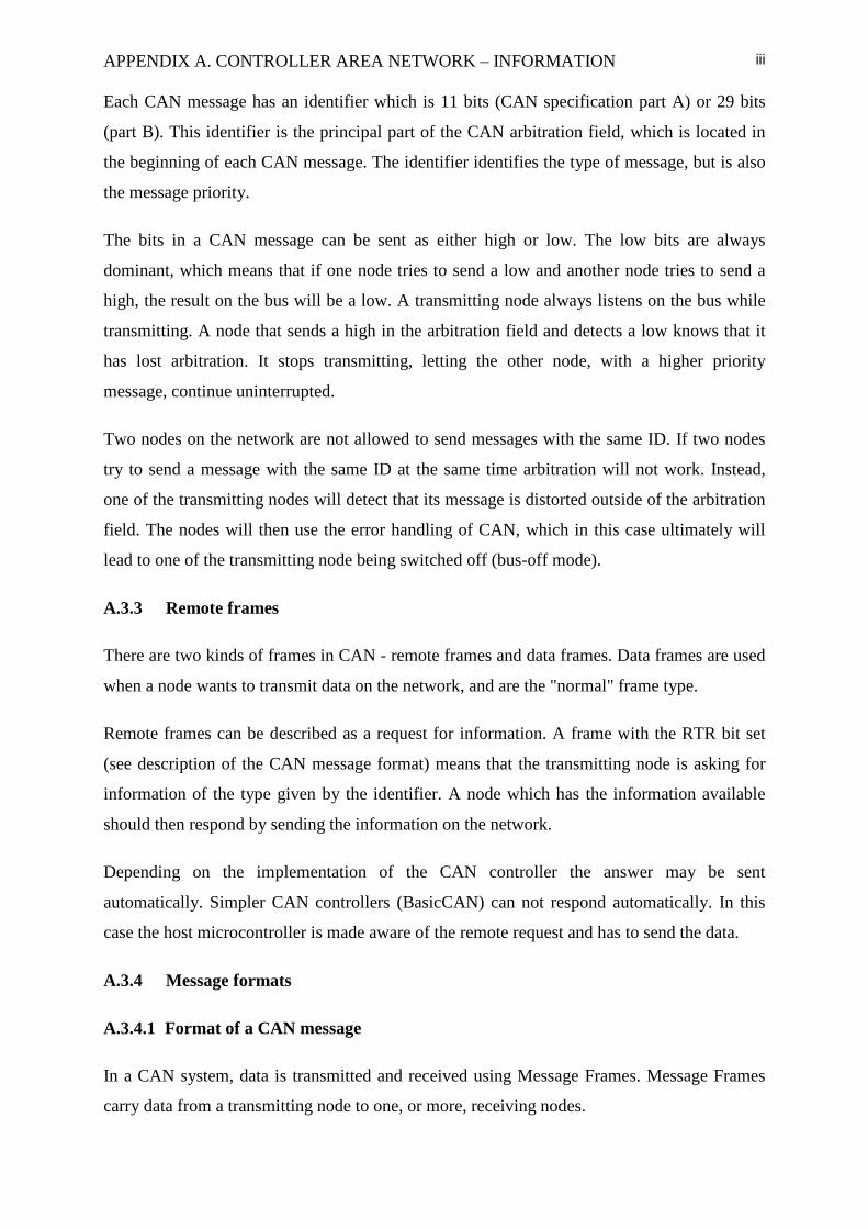
APPENDIX A. CONTROLLER AREA NETWORK – INFORMATION
iii
Each CAN message has an identifier which is 11 bits (CAN specification part A) or 29 bits
(part B). This identifier is the principal part of the CAN arbitration field, which is located in
the beginning of each CAN message. The identifier identifies the type of message, but is also
the message priority.
The bits in a CAN message can be sent as either high or low. The low bits are always
dominant, which means that if one node tries to send a low and another node tries to send a
high, the result on the bus will be a low. A transmitting node always listens on the bus while
transmitting. A node that sends a high in the arbitration field and detects a low knows that it
has lost arbitration. It stops transmitting, letting the other node, with a higher priority
message, continue uninterrupted.
Two nodes on the network are not allowed to send messages with the same ID. If two nodes
try to send a message with the same ID at the same time arbitration will not work. Instead,
one of the transmitting nodes will detect that its message is distorted outside of the arbitration
field. The nodes will then use the error handling of CAN, which in this case ultimately will
lead to one of the transmitting node being switched off (bus-off mode).
A.3.3 Remote frames
There are two kinds of frames in CAN - remote frames and data frames. Data frames are used
when a node wants to transmit data on the network, and are the "normal" frame type.
Remote frames can be described as a request for information. A frame with the RTR bit set
(see description of the CAN message format) means that the transmitting node is asking for
information of the type given by the identifier. A node which has the information available
should then respond by sending the information on the network.
Depending on the implementation of the CAN controller the answer may be sent
automatically. Simpler CAN controllers (BasicCAN) can not respond automatically. In this
case the host microcontroller is made aware of the remote request and has to send the data.
A.3.4 Message formats
A.3.4.1 Format of a CAN message
In a CAN system, data is transmitted and received using Message Frames. Message Frames
carry data from a transmitting node to one, or more, receiving nodes.

APPENDIX A. CONTROLLER AREA NETWORK – INFORMATION
iv
The CAN protocol supports two Message Frame formats.
The two formats are:
- Standard CAN (Version 2.0A)
- Extended CAN (Version 2.0B)
Most 2.0A controllers transmit and receive only Standard format messages, although some
(known as 2.0B passive) will receive extended format messages but then ignore them. 2.0B
controllers can send and receive messages in both formats.
A.3.4.2 CAN 2.0A Format
A Standard CAN (Version 2.0A) Message Frame consists of seven different bit fields:
- A Start of Frame (SOF) field. This is a dominant (logic 0) bit that indicates the beginning of
a message frame.
- An Arbitration field, containing an 11 bit message identifier and the Remote Transmission
Request (RTR) bit. A dominant (logic 0), RTR bit indicates that the message is a Data Frame.
A recessive (logic 1) value indicates that the message is a Remote Transmission Request
(otherwise known as Remote Frame). A Remote Frame is a request by one node for data from
some other nodes on the bus. Remote Frames do not contain a Data Field.
Figure A.1: CAN Version 2.0A Message Frame
Fig CAN 2.0A Message Frame
- A Control Field containing six bits:
* Two dominant bits (r0 and r1) that are reserved for future use, and

APPENDIX A. CONTROLLER AREA NETWORK – INFORMATION
v
* A four bit Data Length Code (DLC). The DLC indicates the number of bytes in the Data
Field that follows
- A Data Field, containing from zero to eight bytes.
- The CRC field, containing a fifteen-bit cyclic redundancy check code and a recessive
delimiter bit.
- The Acknowledge field, consisting of two bits. The first is the Slot bit which is transmitted
as a recessive bit, but is subsequently overwritten by dominant bits transmitted from all other
nodes that successfully receive the message. The second bit is a recessive delimiter bit.
- The End of Frame field, consisting of seven recessive bits.
Following the end of a frame is the Intermission field consisting of three recessive bits. After
the three bit Intermission period the bus is recognized to be free. Bus Idle time may be of any
arbitrary length including zero.
A.3.4.3 CAN 2.0B Format
The CAN 2.0B format provides a twenty nine (29) bit identifier as opposed to the 11 bit
identifier in 2.0A.
Version 2.0B evolved to provide compatibility with other serial communications protocols
used in automotive applications in the USA. To cater for this, and still provide compatibility
with the 2.0A format, the Message Frame in Version 2.0B has an extended format.
The differences are:
- In Version 2.0B the Arbitration field contains two identifier bit fields. The first (the base ID)
is eleven (11) bits long for compatibility with Version 2.0A. The second field (the ID
extension) is eighteen (18) bits long, to give a total length of twenty nine (29) bits.
- The distinction between the two formats is made using an Identifier Extension (IDE) bit.

APPENDIX A. CONTROLLER AREA NETWORK – INFORMATION
vi
Figure A.2: CAN 2.0B Message Format
- A Substitute Remote Request (SRR) bit is included in the Arbitration Field. The SRR bit is
always transmitted as a recessive bit to ensure that, in the case of arbitration between a
Standard Data Frame and an Extended Data Frame, the Standard Data Frame will always have
priority if both messages have the same base (11 bit) identifier.
All other fields in a 2.0B Message Frame are identical to those in the Standard format.
A.3.5 Error detection and fault confinement
The error detection, signaling and fault confinement defined in the CAN standard makes the
CAN bus very reliable. The built in error detection of the controllers together with the error
signaling make sure that the information is correct and consistent. Faulty nodes will go to
modes where they do not disturb the traffic on the bus.
A.3.5.1 The CAN error process
1. The error is detected by the CAN controller (a transmitter or a receiver).
2. An error frame is immediately transmitted.
3. The message is cancelled at all.
4. The status of the CAN controllers are updated
5. The message is re-transmitted. If several controllers have messages to send, normal
arbitration is used.
A.3.5.2 Error detection
Error detection is handled automatically by the CAN controller. The detected errors are:

APPENDIX A. CONTROLLER AREA NETWORK – INFORMATION
vii
• Bit errors:
1. Bit stuffing error - normally a transmitting node inserts a high after five consecutive
low bits (and a low after five consecutive high). This is called bit stuffing. A receiving node
that detects more than five consecutive bits will see a bit stuffing violation.
2. Bit error - A transmitting node always reads back the message as it is sending. If it
detects a different bit value on the bus than it sent, and the bit is not part of the arbitration
field or in the acknowledgement field, an error is detected.
• Message errors:
1. Checksum error - each receiving node checks CAN messages for checksum errors.
2. Frame error - There are certain predefined bit values that must be transmitted at
certain points within any CAN Message Frame. If a receiver detects an invalid bit in one of
these positions a Form Error (sometimes also known as a Format Error) will be flagged.
3. Acknowledgement Error - If a transmitter determines that a message has not been
acknowledged then an ACK Error is flagged.
A.3.5.3 CAN controller error modes
A CAN controller can be in one of three states:
1. Error active - the normal operating mode for a controller. Messages can be received
and transmitted. Upon detecting an error, an active error flag is sent.
2. Error passive - a mode entered when the controller has frequent problems transmitting
or receiving messages. Messages can be received and transmitted. On detecting an error while
receiving, a passive error flag is sent.
3. Bus off - entered if the controller has serious problems with transmitting messages. No
messages can be received or transmitted until the CAN controller is reset by the host
microcontroller or processor.
The state machine is implemented in the CAN controller which determines the mode of the
controller for counters - the transmit error counter and the receive error counter. The
following rules apply:

APPENDIX A. CONTROLLER AREA NETWORK – INFORMATION
viii
1. The CAN controller is in error active mode if transmit is less or equal to 127 and if the
receive count is less or equal to 127.
2. It becomes error passive if transmit error count is greater than 127 but less or equal to
255 or if the receive error count is greater than 127.
3. Bus off is entered if transmit error count is greater than 255.
Once the CAN controller has entered bus off state, it must be reset by the host microcontroller
or processor in order to be able to continue operation. This is shown graphically in figure A.3
Figure A.3: CAN Error States Source: [1], p91, fig. 41-5
A.3.5.4 Error signaling
When an error is detected by a node it sends an error flag on the bus. This prevents any other
node from accepting the message and ensures consistency of data throughout the network.
The active error flag consists of six low bits, and is used if the node transmitting the error
frame is in active error state. As low is dominant all other nodes will detect bit stuffing
violation and send their own error flags. After this, nodes that want to transmit (including the
one sending the interrupted message) will start to do so. As usual, the node whose message
has the highest priority will win arbitration and send its message.
If the CAN controller is in error passive mode the error frame will consist of six passive
(high) bits. Since the error flag only consists of passive bits, the bus is not affected. If no other

APPENDIX A. CONTROLLER AREA NETWORK – INFORMATION
ix
node detected an error, the message will be sent uninterrupted. This ensures that a node
having problems with receiving can not block the bus.
All of this advanced error handling is done automatically by the CAN controller, without any
need for the host microcontroller to do anything. This is one of the big advantages of CAN.
A.3.6 Bit timing
CAN has advanced features for coping with the time delays found in long bus lengths (in
comparison to the bit rate) and coping with differences in clock crystal frequencies for nodes
on the bus.
The choice of bit timing is very important since it decides the bit rate, the sample point and
the ability to resynchronize.
A.3.6.1 Bit segments
Each bit is divided into four segments - the synchronization segment, the propagation segment
and the phase segments one and two. Each segment consists of one or more time quanta.
A time quantum is a fixed amount of time which is derived from the CAN controller clock
with a prescale factor.
Figure A.4: CAN Bit Timing
A.3.6.2 Synchronization segment (Synch_Seg)
The synchronisation segment is used to synchronise the various nodes on the bus. When a bit
is sent on the bus, the leading edge is expected to be within this segment.
This segment is always one time quantum long.
A.3.6.3 Propagation segment (Prop_Seg)
The Propagation Segment is needed to compensate for the delay in the bus lines.

APPENDIX A. CONTROLLER AREA NETWORK – INFORMATION
x
The segment size is programmable between 1 and 8 time quanta.
A.3.6.4 Phase Segment 1 (Phase_Seg1), Phase Segment 2 (Phase_Seg2)
These segments can be used lengthened or shortened by resynchronization.
A.3.7 Resynchronization
Resynchronization is done to compensate for bus delays and nodes that have different crystal
frequencies. Synchronisation is normally only done on the edge from recessive to dominant
bus level.
A.3.7.1 Hard resynchronization
When the bus is idle and the controller detects a start bit, it resynchronizes itself so that the
edge is inside the Synch segment. Hard resynchronization can only be made for the first bit in
a frame.
• Resynchronisation within a frame
CAN controllers have the ability to synchronise on bit edges as well as within a CAN frame.
The (re)Synchronisation Jump Width (SJW) decides the maximum number of time quanta
that the controller can resynchronise every bit.
• Resynchronisation of a receiver to a slower transmitter is handled as follows:
If a recessive-to-dominant edge appears inside TSEG1 and the edge is less than or equal to
SJW quanta inside, TSEG1 is restarted. If the edge was more than SJW quanta inside, TSEG1
is lengthened with SJW quanta.
• Resynchronisation of a receiver to a faster transmitter:
If a recessive-to-dominant edge appears inside TSEG2, TSEG2 is shortened by the number of
quanta necessary to make the edge be outside TSEG2. However, TSEG2 can be shortened no
more than SJW quanta.
A.3.8 CAN bus physical layer
The physical layer is not part of the Bosch CAN standard. However, in the ISO standards
transceiver characteristics is included.

APPENDIX A. CONTROLLER AREA NETWORK – INFORMATION
xi
CAN transmits signals on the CAN bus which consists of two wires, a CAN-High and CAN-
Low. These 2 wires are operating in differential mode; that is they are carrying inverted
voltages (to decrease noise interference). The voltage levels, as well as other characteristics of
the physical layer, depend on which standard is being used.
A.3.8.1 ISO 11898
The voltage levels for a CAN network which follows the ISO 11898 (CAN High Speed)
standard are listed in table.
Table A.1: CAN Bus Voltage Levels
Signal Recessive State (Volts) Dominant State (Volts)
Level Min Nominal Max Min Nominal Max
CAN-High 2.0 2.5 3.0 2.75 3.5 4.5
CAN-Low 2.0 2.5 3.0 0.5 1.5 2.25
Note that for the recessive state, nominal voltage for the two wires is the same. This decreases
the power drawn from the nodes through the termination resistors. These resistors are 120 Ω
and are located on each end of the wires.
A.3.8.2 ISO 11519
The voltage levels for a CAN network which follows the ISO 11519 (CAN Low Speed)
standard are described in the table below.
Table A.2: CAN Bus Voltage Levels
Signal Recessive State (Volts) Dominant State (Volts)
Level Min Nominal Max Min Nominal Max
CAN-High 1.6 1.75 1.9 3.85 4.0 5.0
CAN-Low 3.1 3.25 3.4 0 1.0 1.15
ISO 115519 does not require termination resistors. They are not necessary because the limited
bit rates (maximum 125 kbps) make the bus insensitive to reflections.

APPENDIX A. CONTROLLER AREA NETWORK – INFORMATION
xii
The voltage level on the CAN bus is recessive when the bus is idle.
A.3.9 Bus lengths
The maximum bus length for a CAN network depends on the bit rate used. It is required that
the wave front of the bit signal has time to travel to the most remote node and back again
before the bit is sampled. This means that if the bus length is near the maximum for the bit
rate used, one should choose the sampling point with utmost care.
Below is a table of different bus lengths and the corresponding maximum bit rates.
Table A.3: Practical Maximum Bus Lengths
A.3.10 Media
According to the ISO 11898 standard, the impedance of the cable shall be 120 +- 12 Ω. It
should be twisted pair, shielded or unshielded. Work is in progress on the single-wire standard
SAE J2411.
A.3.11 CAN implementations
• Different implementations - BasicCAN and FullCAN
There is no standard on how CAN controllers shall be implemented or how they shall
communicate with their host microcontroller. There are two main implementation strategies
for CAN controllers today. They are called BasicCAN and FullCAN.
The main difference between these strategies is how interesting messages are filtered out, that
is how it is decided what messages are interesting and which are not. There are also
differences in how remote frames are answered, and on how messages are buffered. The
differences will effect how much load is put on the host microcontroller.

APPENDIX A. CONTROLLER AREA NETWORK – INFORMATION
xiii
• BasicCAN
BasicCAN is usually used in cheaper standalone CAN controllers or in smaller
microcontrollers with integrated CAN controller.
A BasicCAN controller normally has two receive buffers and one transmit buffer. The receive
buffers are arranged in a FIFO structure, and a message can be received into one buffer while
the microcontroller is reading the information from the other buffer. If a message is received
while both receive buffers are full, the oldest messages are kept. This means that newer
messages might be lost if the host microcontroller does not read the messages fast enough.
A message is sent by writing it to the transmit buffer.
Interesting messages are filtered out using two registers that operate on the message identifier.
Each bit in the identifier is checked against the filter. If the message matches the filter it is
stored in one of the receive buffers.
Each bit of the identifier filter can be set to '1', '0' or 'don't care'. Often the filter only operates
on eight of the eleven bits in the identifier (standard CAN). This means the three lower bits in
the identifier are always 'don't care'.
When BasicCAN is used it is important to choose identifiers with utmost care, so that the
window of the filter can be kept as small as possible. All messages that are let through the
filter must be read and checked by the microcontroller. This means that the final filtering is
done in software.
A BasicCAN controller has no support for automatically answering remote frames, which
means that the application will have to handle them. This will put extra load on the
microcontroller or processor, but will make sure that the value returned is updated.

APPENDIX A. CONTROLLER AREA NETWORK – INFORMATION
xiv
Table A.4: BasicCAN features
Transmit The application fills complete Tx register Including ID,RTR, data length,
data: every ID can be transmitted
Receive Every masked CAN message can be received. Normally two receive
buffers in FIFO structure Global message filtering. It is normally not
possible to set up the filter so that only the interesting messages are let
through: final filtering must be done by the application
Remote Frame
handling
Remote frames are answered by the application
Overrun
philosophy
Keep the oldest message (newer messages will be lost)
• FullCAN
FullCAN is used in more expensive, high performance CAN controllers and microcontrollers.
The FullCAN controller has a set of buffers called mailboxes. On initialization, each mailbox
is assigned an identifier and is set to transmit or receive.
When the CAN controller receives a message it checks the mailboxes in order to see if there is
a receive mailbox with the same identifier as the message. If such a mailbox is found, the
message is stored in it and the host controller is notified. Otherwise the message is discarded.
When transmitting a message, the message length and data is written to the transmit mailbox
with the correct identifier.
If a remote message is received the controller checks the remote identifier against the transmit
mailboxes. If a match is found, the controller automatically sends a message with the
identifier and data contained in that mailbox. This means that the microcontroller gets a lower
load, and that the software does not have to handle remote messages. However, if the mailbox
has not been updated in a long time, the information sent to the network will be old. This has
to be considered when writing the software.
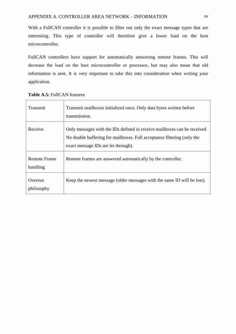
APPENDIX A. CONTROLLER AREA NETWORK – INFORMATION
xv
With a FullCAN controller it is possible to filter out only the exact message types that are
interesting. This type of controller will therefore give a lower load on the host
microcontroller.
FullCAN controllers have support for automatically answering remote frames. This will
decrease the load on the host microcontroller or processor, but may also mean that old
information is sent. It is very important to take this into consideration when writing your
application.
Table A.5: FullCAN features
Transmit Transmit mailboxes initialized once. Only data bytes written before
transmission.
Receive Only messages with the IDs defined in receive mailboxes can be received
No double buffering for mailboxes. Full acceptance filtering (only the
exact message IDs are let through).
Remote Frame
handling
Remote frames are answered automatically by the controller.
Overrun
philosophy
Keep the newest message (older messages with the same ID will be lost).

Appendix B
CAN Baud Rate Setting
A method for CAN baud calculations that uses the AT90CAN128 data sheet CAN example
baud rate settings as a basis is presented here. A desired AVR clock speed and baud rate must
be specified, then use the examples to get the Tprs, Tph1, Tph2 and Tsjw values.
Looking at the AT90CAN128 data sheet, page 266 section 19.12, Examples of CAN Baud
Rate Setting, note the CAN Baud Rate, TQ and Tbit columns. It should be noticed that if you
convert TQ into seconds: BAUD = 1 / (TQ * Tbit)
Using simple algebra we get this formula for the Time Quanta (TQ) value:
TQ = 1 / (BAUD * Tbit)
Because Tbit must be 8 or higher, an 8 MHz clock is the slowest possible AVR clock for the
maximum 1 mega-baud CAN operation (8000000 / 8 = 1000000). Also because the maximum
AVR clock is 16 MHz (1 / 16000000 = 6.25 E-8), the smallest TQ possible (within the AVR
specifications) with prescaler BRP [5:0] = 0 is 0.0625 microseconds (6.25 E-8seconds).
As per the CAN specification, Tbit must be at least from 8 to 25.
If you pick a desired baud rate, then use Tbit = 8 you can calculate the required TQ which we
will call TQ8: TQ8 = 1 / (BAUD * 8)
Then use Tbit = 25 and calculate the required TQ which we will call TQ25 (so you have a
range of possible TQ values). TQ25 = 1 / (BAUD * 25)
Examine TQ8 and TQ25 to make sure they are equal or larger than CLKio (your AVR I/O
clock is the AVR speed taking CLKPR and CKDIV8 into account) divided into 1. Any TQ
value for a given Tbit (8 to 25) value that is too small means it cannot be used. For an
example, look at the data sheet 8 MHz clock in 19.12 Examples of CAN Baud Rate Setting.
You will see that at 1 mega-baud an 8 MHz AVR I/O clock is 0.125 microseconds and it
matches a TQ8 of 0.125 microseconds. A TQ9 is 0.11111 microseconds, which is a smaller

APPENDIX B. CAN BAUD RATE SETTING
xvii
value than the AVR CLKio which is as fast as the AVR can go at that clock speed. So, TQ9 is
too small to be used at this baud rate and CLKio speed. Do not try to use any Tbit values that
do not meet the time quanta limitations.
Next take your CLKio frequency (AVR system clock divided by the CLKPR value) and
multiply it by TQ8: TDIV8 = (CLKio * TQ8) – 1
Round TDIV8 off to an integer. This will be the required prescaler divider BRP [5:0] bit
value in decimal. Because BRP [5:0] is only 6 binary bits, TDIV8 must always be in the 0 and
63 decimal value range. If TDIV8 is larger than 63 decimal it means you cannot set the
BRP[5:0] to a high enough value for that baud rate at Tbit = 8. You could use CLKPR to
reduce CLKio if you really wanted to use Tbit = 8 for some reason.
Now you can do: TDIV25 = (CLKio * TQ25) – 1 and round it off to an integer (it must also
be 0 to 63 or it cannot be used).
What TDIV8 and TDIV25 tell you is what range of BRP [5:0] prescaler values are possible
for your desired baud rate. When rounding off the TDIV8 and TDIV25 prescaler values
recalculate the TQ values: TQ8 = TDIV8 + 1 / CLKio
TQ25 = TDIV25 + 1 / CLKio
Note that the original TQ8 and TQ25 values may change in the above formulas because of the
TDIV8 and TDIV25 round off.
Next there is something else the data sheet that 19.12 Examples of CAN Baud Rate Setting
can teach us. You will notice that: Tbit = Tsyns + Tprs + Tphs1 + Tphs2
Tsyns is the built in 1 TQ long synchronization bit, so its value is fixed as a 1 at all times
which gives us: Tbit = 1 + Tprs + Tphs1 + Tphs2
In fact there is a pattern in the examples table. The Tprs, Tph1, Tph2 and Tsjw values are
always the same for a given Tbit value (it does not matter what the clock speed or baud rate
is). We can take a shortcut here and copy the pattern values for a new baud rate that is not in
the table. The data sheet has Tbit values for 20, 16, 15, 12, 10 and 8. So, using your custom
baud rate pick one of these Tbit values and calculate your TQ. Then use CLKio and TQ to
calculate your prescaler division integer. If the prescaler division calculation does not need
rounding off into an integer, your baud rate will be perfect. If there is any remainder to round
off your baud rate will not be perfect (use the first formula to figure out your actual BAUD

APPENDIX B. CAN BAUD RATE SETTING
xviii
rate). Lastly, copy the Tprs, Tph1, Tph2 and Tsjw values (CANBT2 and CANBT3) for the
same Tbit value as the one you used. This is method to quickly setup what should be a
workable CAN baud setting for CANBT1, CANBT2 and CANBT3 using a custom baud rate
or custom AVR system clock frequency.
Here is a 9600 baud example with an AVR 7.3728 MHz system clock and CLKPR of 0 (i.e.
CLKio = 7.3728 MHz).
TQ = 1 / (BAUD * Tbit)
TQ8 = 1 / (9600 * 8) = 1.302 E-05
TQ25 = 1 / (9600 * 25) = 4.166 E-06
TDIV = (CLKio * TQ) – 1
TDIV8 = (7372800 * 1.302 E-05) – 1 = 95
TDIV25 = (7372800 * 4.166 E-06) – 1 = 29.72 (rounded to 30)
Notice that a TDIV8 of 95 exceeds the BRP [5:0] maximum value of 63, so it is not usable.
However, since TDIV25 is under the 63 maximum value we know it is possible to use other
Tbit values higher than 8. Since we have to pick from the existing table 20, 16, 15, 12, 10
selection, lets just go to Tbit = 16.
TQ16 = 1 / (9600 * 16) = 6.510 E-06
TDIV16 = (7372800 * 6.510 E-06) – 1 = 47
There is no remainder in TDIV16, so 9600 baud is a perfect baud rate at this AVR clock
speed with Tbit set to 16. If we double check, even though we do not have to because of the
perfect baud rate match:
TQ16 = (TDIV16 + 1) / CLKio
TQ16 = (47 + 1) / 7372800 = 6.510 E-06
This tells us BRP [5:0] = 47 decimal which is 101111 binary and formats into CANBT1 as
1011110 binary or 0x5E hex.
Then we just take the existing Tprs, Tph1, Tph2 and Tsjw values for Tbit = 16. So, we get:

APPENDIX B. CAN BAUD RATE SETTING
xix
CANBT1 = 0x5E
CANBT2 = 0x0C
CANBT3 = 0x37
A general alternative to the method above for all microcontrollers is a CAN calculator that
can be downloaded from a free website [11]. In this calculator you just put the baud rate and
the clock frequency and the calculator will compute the CAN bit timing values with all
possible combinations.

APPENDIX C. SOURCE CODE
xx
Appendix C
Source Code

APPENDIX C. SOURCE CODE
xxi
canprotocol_main.c

APPENDIX C. SOURCE CODE
xxii
can_msg_drv.c

APPENDIX C. SOURCE CODE
xxiii
candriv.c

APPENDIX C. SOURCE CODE
xxiv
canTimer.c

APPENDIX C. SOURCE CODE
xxv
adc_mlib.c

APPENDIX C. SOURCE CODE
xxvi
sensor_drv.c

APPENDIX C. SOURCE CODE
xxvii
canDemo.c