a 3-dimensional well model in the flow transport through porous media

Applied Mathematical Modelling xxx (2014) xxx–xxx

Contents lists available at ScienceDirect

Applied Mathematical Modelling

journal homepage: www.elsevier .com/locate /apm

A 3-dimensional well model in the flow transport throughporous media

http://dx.doi.org/10.1016/j.apm.2014.03.0450307-904X/� 2014 Elsevier Inc. All rights reserved.

⇑ Tel.: +869318912483.E-mail address: [email protected]

1 The author was supported by the Fundamental Research Funds for the Central Universities.

Please cite this article in press as: T. Zhang, A 3-dimensional well model in the flow transport through porous media, Appl. Math.(2014), http://dx.doi.org/10.1016/j.apm.2014.03.045

Ting Zhang ⇑,1

School of Mathematics and Statistics, Lanzhou University, Lanzhou, Gansu 730000, PR China

a r t i c l e i n f o

Article history:Received 24 November 2012Received in revised form 19 November 2013Accepted 25 March 2014Available online xxxx

Keywords:Well modelError estimateNumerical algorithm

a b s t r a c t

In petroleum extraction and exploitation, the well is usually treated as a point or linesource, due to its radius is much smaller comparing with the scale of the whole reservoir.Especially, in 3-dimensional situation, the well is regarded as a line source. In this paper,we analyze the modeling error for this treatment for steady flows through porous mediaand present a new algorithm for line-style well to characterize the wellbore flow potential.We also provide a numerical example to demonstrate the effectiveness of the proposedmethod.

� 2014 Elsevier Inc. All rights reserved.

1. Introduction

In many practical applications, especially by resistivity well-logging in petroleum exploitation, the boundary value prob-lem with equivalued surfaces is formulated, see [1–4] for instance. From the physical view, the equivalued surface boundarycorresponds to a source in the reservoirs. In 2-dimensional case, the equivalued surface boundary can be regarded as a point.So this type of source reduces to a point source, and the modeling error has been discussed by Chen–Yue [5]. In 3-dimen-sional situation, the equivalued surface boundary can be treated as a line rather than a point. One main aim of the presentpaper is to derive the modeling error in 3-dimensional case.

Consider a vertical well in R3. Let X ¼ H� ða; dÞ � R3 be a cylinder-like domain, where H � R2 is a bounded domain. For apoint ðx0; y0Þ 2 H, denote by Bd the small disk contained in H with center ðx0; y0Þ and radius d. Let Bd � ða; dÞ be the domainthat occupied by the well. Set Hd ¼ H n Bd and Xd ¼ Hd � ða; dÞ. We consider the following single phase potential equationwhich is formed by combining Darcy’s Law with conversation of mass

�divðKrudÞ ¼ 0 in Xd;

where ud is the flow potential, K is the permeability. We will impose mixed boundary conditions

udj@H�ða;dÞ ¼ 0;@ud

@m

��Hd�fa;dg

¼ 0;

on the exterior boundary. On the well boundary @Bd � ða; dÞ, two quantities are of particular importance in practicalapplications: the wellbore potential uj@Bd�ða;dÞ and the well flow rate

R@Bd�fzg K @ud

@m ds ðz 2 ða; dÞÞ, where m is the unit outer

Modell.

http://dx.doi.org/10.1016/j.apm.2014.03.045

mailto:[email protected]


http://www.sciencedirect.com/science/journal/0307904X

http://www.elsevier.com/locate/apm


2 T. Zhang / Applied Mathematical Modelling xxx (2014) xxx–xxx

normal to Xd. In practice, the well is only open in part segment. Let ½a; d� ¼ ½a; b� [ ðb; cÞ [ ½c; d�. Suppose that the well is openin ðb; cÞ and closed in ½a; b� [ ½c; d�. Therefore we set up two kinds of boundary conditions for the wellbore boundary. Namelywe assume that the layer flow rate is fixed in ðb; cÞ and no flow rate in ½a; b� [ ½c; d�, i.e.

Please(2014

udj@Bd�fzg ¼ lðzÞ ðunknownÞ;Z@Bd�fzg

K@ud

@mds ¼ qðzÞ; z 2 ða;dÞ;

where lð�Þ is a unknown function which depends only the height z of the well and qðzÞ is defined by

qðzÞ ¼qðzÞ z 2 ðb; cÞ;0 z 2 ½a; b� [ ½c;d�:

�ð1:1Þ

In this paper, we mainly consider the following boundary value problem

�divðKðx; y; zÞrudÞ ¼ 0 ðx; y; zÞ 2 Xd;

udj@H�ða;dÞ ¼ 0;@ud@m jHd�fa;dg ¼ 0;

udj@Bd�fzg ¼ l0ðzÞ ðunknownÞ;R@Bd�fzg K @ud

@m ds ¼ qðzÞ; z 2 ða; dÞ;

8>>>><>>>>:

ð1:2Þ

where qðzÞ is defined in (1.1).Since the size of the well d is negligible in practical situations, the approximation of problem (1.2) is as follows

�divðKðx; y; zÞruÞ ¼ qðzÞdl ðx; y; zÞ 2 X;

uj@H�½a;d� ¼ 0;@u@m jH�fa;dg ¼ 0:

8><>: ð1:3Þ

Here qðzÞ is the flow rate mentioned in (1.2), and dl is the line-style Dirac measure at fðx0; y0; zÞ; z 2 ðb; cÞg defined by
ZX
f ðx; y; zÞdldX ¼Z c

bf ðx0; y0; zÞdz; 8f 2 CðXÞ:

The first result of this paper is the following error estimate between the exact solution ud and the approximate solution u, i.e.

maxx2�Xd

ju� udj 6 Cdj ln dj;

where the constant C is independent of d. As far as we know, this is the first result in 3-dimensional case. The proof dependson a sharp estimate between the well flow rate and the wellbore potential.

Next we develop a new algorithm to get the wellbore potential on mesh h� d. The main idea of our algorithm is to indi-cate the wellbore flow by proposing a quantity named equivalent flow potential (EFP) 1

b�c

R cb uj@Bd

dz (where u is the flowpotential, ðb; cÞ is the height of well, and @Bd � ðb; cÞ is the wellbore boundary). We first solve the problem (1.3) by finiteelement method and then obtain the discrete solution uh. It is well known that uh fails to give good approximation in thevicinity of well singularity. One way to overcome this difficulty is to introduce a auxiliary function w ¼ u� w, where

w ¼ 14pK0

R da

q0ðlÞffiffiffiffiffiffiffiffiffiffiffiffiffiffiffiffiffiffiffiffiffiffiffiffiffiffiffiffiffiffiffiffiffiffiffiðx�x0Þþðy�y0Þ2þðz�lÞ2p dl is the singular function.

Since w is regular, we can do accurate approximation for w. Denote by wh 2 Vh the finite element approximation of w.

Thus the value of uh on the well boundary Cd ¼ fðx; y; zÞ :

ffiffiffiffiffiffiffiffiffiffiffiffiffiffiffiffiffiffiffiffiffiffiffiffiffiffiffiffiffiffiffiffiffiffiffiffiffiffiffiffiffiffiffiðx� x0Þ2 þ ðy� y0Þ

2q

¼ d; z 2 ðc; dÞg can be approximated by

uhjCd¼ whðx0; y0; zÞ þ wj@Bd

:

Furthermore,R c

b uj@Bddz can be approximated by

�ah ¼Z c

bwhðx0; y0; zÞdzþ

Z c

bwj@Bd

dz:

Our method improves the computational efficiency because we only use a quantity named EFP to characterize the well-bore pressure instead of correcting the wellbore potential at every layer.

The rest of the paper is organized as follows. In Section 2, we prove the error estimate between the exact solution and theapproximate solution. In Section 3, we introduce our new algorithm and verify the convergence property of this algorithm. InSection 4, we give some numerical results to demonstrate the accuracy of our proposed method. We end the paper withsome concluding remarks.

2. The modeling error

Let D � X be a subdomain with Lipschitz boundary. For each integer m P 0 and 1 6 p 6 þ1, we denote by Wm;pðDÞ thestandard Sobolev space of real functions having all their weak derivatives up to order m in the Lebesgue space LpðDÞ. The

cite this article in press as: T. Zhang, A 3-dimensional well model in the flow transport through porous media, Appl. Math. Modell.), http://dx.doi.org/10.1016/j.apm.2014.03.045


T. Zhang / Applied Mathematical Modelling xxx (2014) xxx–xxx 3

norm and the semi-norm of Wm;pðDÞ will be denoted by k � km;p;D and j � jm;p;D, respectively. As usual, Wm;2ðDÞ is denoted byHmðDÞ with norm k � km;D and semi-norm j � jm;D.

The main purpose of this section is to derive the pointwise error estimate between the solutions ud and u. The followingtheorem is the main result of this section.

Theorem 2.1. Assume that K � K0 > 0 is a constant function and q 2 C1ð½a; d�Þ with qðbÞ ¼ qðcÞ ¼ 0. Let ud and u be solutions of(1.2) and (1.3), respectively. Then there exists a constant C independent of d such that

Please(2014

maxx2�Xd

ju� udj 6 Cdj ln dj:

Proof. For clarity, we divide the proof into four steps.

Step 1. We first derive the equation satisfied by ud � u.If w is the solution of

�divðK0rwÞ ¼ qðzÞdl ðx; y; zÞ 2 R3;

w! 0 as ðx; y; zÞ ! 1;

(

then

w ¼ 14pK0

Z d

a

qðlÞffiffiffiffiffiffiffiffiffiffiffiffiffiffiffiffiffiffiffiffiffiffiffiffiffiffiffiffiffiffiffiffiffiffiffiffiffiffiffiffiffiffiffiffiffiffiffiffiffiffiffiffiffiffiffiffiffiffiffiffiffiffiðx� x0Þ þ ðy� y0Þ

2 þ ðz� lÞ2q dl: ð2:1Þ

Let wd ¼ ud � w and let w ¼ u� w. Then the function vd ¼ ud � u ¼ wd �w satisfies

�divðK0rvdÞ ¼ 0 ðx; y; zÞ 2 Xd;

vdj@H�ða;dÞ ¼ 0;@vd@m jHd�fa;dg ¼ 0;

vdj@Bd�fzg ¼ ðud � uÞj@Bd�fzg ¼ lðzÞ �wj@Bd�fzg � wj@Bd�fzg; ðlðzÞ is unknownÞR@Bd�fzg K0

@vd@m ds ¼ qðzÞ �

R@Bd�fzg K0

@u@m ds; z 2 ða;dÞ:

8>>>>>>><>>>>>>>:

In order to estimate kvdkL1ð�XdÞ, we split vd into two parts

vd ¼ v1 þ v2;

where v1;v2 satisfy

�divðK0rv1Þ ¼ 0 ðx; y; zÞ 2 Xd;

v1j@H�ða;dÞ ¼ 0;@v1@m jHd�fa;dg ¼ 0;

v1j@Bd�fzg ¼ wðx0; y0; zÞ �wj@Bd�fzg; z 2 ða; dÞ

8>>>><>>>>:

and

�divðK0rv2Þ ¼ 0 ðx; y; zÞ 2 Xd;

v2j@H�ða;dÞ ¼ 0;@v2@m jHd�fa;dg ¼ 0;v2j@Bd�fzg ¼ lðzÞ �wðx0; y0; zÞ � wj@Bd�fzg;R@Bd�fzg K0

@v2@m ds ¼ qðzÞ �

R@Bd�fzg K0

@v1@m ds�

R@Bd�fzg K0

@u@m ds; z 2 ða; dÞ;

8>>>>>>><>>>>>>>:

respectively.Step 2. We give the bound of kv1kL1ð�XdÞ.To achieve this purpose, we only need to bound

maxx2@Bd�fzg

wðx0; y0; zÞ �wðx; y; zÞj j:

Note that w ¼ u� w satisfies

�divðK0rwÞ ¼ 0 ðx; y; zÞ 2 X;

wj@H�ða;dÞ ¼ �wj@H�ða;dÞ;@w@m jHd�fa;dg ¼ �

@w@m jHd�fa;dg:

8><>:




It is obvious that w 2 C2ð�XÞ. Then we have

Please(2014

maxx2@Bd�fzg

wðx0; y0; zÞ �wðx; y; zÞj j 6 CdkrwkC0ð�XÞ 6 Cd:

By maximum principle, we obtain

kv1kL1ð�XdÞ 6 maxx2@Bd�fzg

wðx0; y0; zÞ �wðx; y; zÞj j 6 Cd:

Step 3. We estimate the flow rate of v2, i.e.
Z@Bd�fzg
K0@v2

@mds ¼ �

Z@Bd�fzg

K0@v1

@mdsþ qðzÞ �

Z@Bd�fzg

K0@u@m

ds; z 2 ða;dÞ: ð2:2Þ

Let us deal with the first term on the right-hand side of (2.2). Set wðx0; y0; zÞ �wj@Bd�fzg ¼ dbðzÞ, where jbðzÞj 6 C. Letv1 ¼ dp. Then the function p satisfies the following problem

�divðK0rpÞ ¼ 0 ðx; y; zÞ 2 Xd;

pj@H�ða;dÞ ¼ 0;@p@m jHd�fa;dg ¼ 0;

pj@Bd�fzg ¼ bðzÞ; z 2 ða; dÞ;

8>>>><>>>>:

By Gilbarg–Trudinger [6], we know that @p@m

�� @Bd�fzg

6 C. Hence,
Z@Bd�fzg
@v1

@mds

�� 6 Cd

Z@Bd�fzg

@p@m

ds��

�� 6 CdZ@Bd�fzg

@p@m

��ds 6 Cd:

For the term qðzÞ �R@Bd�fzg K0

@u@m ds in (2.2), we have

qðzÞ �Z@Bd�fzg

K0@u@m

ds��

�� ¼ qðzÞ þZ@Bd�fzg

K0@u@r

ds��

�� 6 jqðzÞ þZ@Bd�fzg

K0@w@r

dsj þZ@Bd�fzg

K0@w@r

ds��

��6 qðzÞ � 1

2

Z d

a

d2qðlÞ

ðd2 þ ðz� lÞ2Þ32

dl

��þ Cd2 ¼ qðzÞ � 1

2

Z c

b

d2qðlÞ


dl

��þ Cd2: ð2:3Þ

Let us estimate the right-hand side of (2.3). Direct calculation shows that

qðzÞ � 12

Z c

b

d2qðlÞ


dl

�� 6 jqðzÞj 1� 1

2

Z c

b

d2


dl

��þ

12

Z c

b

d2ðqðzÞ � qðlÞÞ


dl

��

6 jqðzÞj 1þ 12

z� cffiffiffiffiffiffiffiffiffiffiffiffiffiffiffiffiffiffiffiffiffiffiffiffiffiffiffid2 þ ðz� cÞ2

q � z� bffiffiffiffiffiffiffiffiffiffiffiffiffiffiffiffiffiffiffiffiffiffiffiffiffiffiffid2 þ ðz� cÞ2

q0B@

1CA

��þ

12

maxn2ðb;cÞ

jq0ðnÞjZ c

b

ðz� lÞd2


dl

��

612jqðzÞj 1þ z� cffiffiffiffiffiffiffiffiffiffiffiffiffiffiffiffiffiffiffiffiffiffiffiffiffiffiffi

d2 þ ðz� cÞ2q

��þ

12jqðzÞj 1� z� bffiffiffiffiffiffiffiffiffiffiffiffiffiffiffiffiffiffiffiffiffiffiffiffiffiffiffi

d2 þ ðz� bÞ2q

��

þ 12

d2 maxn2ðb;cÞ

jq0ðnÞj 1ffiffiffiffiffiffiffiffiffiffiffiffiffiffiffiffiffiffiffiffiffiffiffiffiffiffiffid2 þ ðz� cÞ2

q � 1ffiffiffiffiffiffiffiffiffiffiffiffiffiffiffiffiffiffiffiffiffiffiffiffiffiffiffiðz� bÞ2 þ d2

q��

�� , Iþ IIþ III:

Let us estimate the term I. We get the estimate by two cases.

Case 1: z 2 ½a; b� [ ½c; d�.It is easy to get I ¼ 0 due to qðzÞ ¼ 0 when z 2 ½a; b� [ ½c; d�.

Case 2: z 2 ðb; cÞ.Since q 2 C1ð½a; d�Þ and qðcÞ ¼ 0, we have qðzÞ ¼ q0ðnÞðz� cÞ, here n 2 ðz; cÞ. Hence

I 612

maxn2ðb;cÞ

jq0ðnÞjðc � zÞ 1� c � zffiffiffiffiffiffiffiffiffiffiffiffiffiffiffiffiffiffiffiffiffiffiffiffiffiffiffid2 þ ðz� cÞ2

q0B@

1CA:

By direct calculation, we get that




Please(2014

ðc � zÞ 1� c � zffiffiffiffiffiffiffiffiffiffiffiffiffiffiffiffiffiffiffiffiffiffiffiffiffiffiffid2 þ ðz� cÞ2

q0B@

1CA 6 Cd:

Hence

I 6 Cd;

where the constant C is independent of d.

In a similar way, we get II 6 Cd. It is clear that III 6 Cd. Combining the above estimates, we obtain
Z@Bd�fzg
K0@v2

@mds

�� 6 Cd:

Step 4. We shall estimate kv2kL1ð�XdÞ.Denote

QðzÞ ¼Z@Bd�fzg

K0@v2

@mds ¼ QþðzÞ � Q�ðzÞ; z 2 ða; dÞ:

Here QðzÞ ¼maxfQðzÞ;0g. If we let q1 ¼ maxz2ða;dÞQþðzÞ and let q2 ¼ �minz2ða;dÞQ

�ðzÞ, then jq1;2j 6 Cd.Let v2;1 satisfy

�divðK0rv2;1Þ ¼ 0 ðx; y; zÞ 2 Xd;

v2;1j@H�ða;dÞ ¼ 0;@v2;1@m jHd�fa;dg ¼ 0;

v2;1j@Bd�fzg depends only on z;R@Bd�fzg K0

@v2;1@m ds ¼ q1; z 2 ða;dÞ

8>>>>><>>>>>:

and let v2;2 satisfy

�divðK0rv2;2Þ ¼ 0 ðx; y; zÞ 2 Xd;

v2;2j@H�ða;dÞ ¼ 0;@v2;2@m jHd�fa;dg ¼ 0;

v2;2j@Bd�fzg depends only on z;R@Bd�fzg K0

@v2;2@m ds ¼ q2; z 2 ða;dÞ:

8>>>>><>>>>>:

We aim at to prove that v2;2 6 v2 6 v2;1. Set �v ¼ v2 � v2;1. Then �v satisfies

�divðK0r�vÞ ¼ 0 ðx; y; zÞ 2 Xd;

�v@H�ða;dÞ ¼ 0;@�v@m jHd�fa;dg ¼ 0;

�v j@Bd�fzg depends only on z;R@Bd�fzg K0

@�v@m ds P 0; z 2 ða;dÞ:

8>>>><>>>>:

Then we have �v 6 0. If not, there exists w0 2 @Bd � fzg such that �vðw0Þ ¼maxw2@Bd�fzg�vðwÞ. By Hopf’s Lemma, we get@�v@m ðw0Þ 6 0. This is a contraction. Hence v2 6 v2;1. Similarly, we have v2;2 6 v2.

The next stage is to bound v2;1 and v2;2. Define

R1 ¼ minðx;y;zÞ2@H�fzg


2q

; z 2 ða;dÞ;

~Xd ¼ ðBR1 n BdÞ � ða;dÞ;

where BR1 denotes the circle in R2 with center ðx0; y0Þ and radius R1.Let �v2;1 satisfy

�divðK0r�v2;1Þ ¼ 0 ðx; y; zÞ 2 ~Xd;

�v2;1j@BR1�ða;dÞ ¼ 0;

@�v2;1@m jðBR1

nBdÞ�fa;zg ¼ 0;

�v2;1 depends only on z;R@Bd�fzg K0

@�v2;1@m ds ¼ q1; z 2 ða; dÞ;

8>>>>>><>>>>>>:

ð2:4Þ

we get by Hopf’s Lemma that �v2;1 6 0. Set ~v ¼ v2;1 � �v2;1. Then ~v satisfies




Please(2014

�divðK0r~vÞ ¼ 0 ðx; y; zÞ 2 ~Xd;

~vj@BR1�ða;dÞ ¼ v2;1;

@~v@m jðBR1

nBdÞ�fa;zg ¼ 0;

~vj@Bd�fzg depends only on z;R@Bd�fzg K0

@~v@m ds ¼ 0; z 2 ða; dÞ:

8>>>>><>>>>>:

By compare principle, we have ~v2 6 0. Hence v2;1 6 �v2;1.In a similar way, let �v2;2 satisfy

�divðK0r�v2;2Þ ¼ 0 ðx; y; zÞ 2 X̂d;

�v2;2j@BR2�ða;dÞ ¼ 0;

@�v2;2@m jðBR2

nBdÞ�fa;zg ¼ 0;

�v2;2j@Bd�fzg depends only on z;R@Bd�fzg K0

@�v2;2@m ds ¼ q2; z 2 ða;dÞ;

8>>>>>><>>>>>>:

ð2:5Þ

where R2 ¼maxðx;y;zÞ2@H�fzgffiffiffiffiffiffiffiffiffiffiffiffiffiffiffiffiffiffiffiffiffiffiffiffiffiffiffiffiffiffiffiffiffiffiffiffiffiffiffiffiffiffiffiðx� x0Þ2 þ ðy� y0Þ

2q

; z 2 ða; dÞ and X̂d ¼ ðBR2 n BdÞ � ða; dÞ, the definition of BR2 is similar as BR1 ’sin the above text. Then we have �v2;2 6 v2;2 6 v2 6 v2;1 6 �v2;1.

Up to now, it suffices to bound k�v2;1kL1ðXdÞ and k�v2;2kL1ðXdÞ. Note that (2.4) can be rewritten as the following form

�K01r ð

@�v2;1@r ðr

@�v2;1@r ÞÞ þ

@2 �v2;1@z2

� �¼ 0 ðr; zÞ 2 ðd;R1Þ � ða;dÞ;

�v2;1jR1�ða;dÞ ¼ 0;@�v2;1@z jðr;R1Þ�fa;dg ¼ 0;

� r @�v2;1@r

� ��r¼d¼ q1

2pK0:

8>>>>>><>>>>>>:

Hence, we have �v2;1 ¼ � q12pK0

ln rR1

. Similarly, problem (2.5) is equivalent to

�K01r ð

@�v2;2@r ðr

@�v2;2@r ÞÞ þ

@2 �v2;2

@z2

� �¼ 0 ðr; zÞ 2 ðd;R2Þ � ða;dÞ;

�v2;2jR2�ða;dÞ ¼ 0;@�v2;2@z jðd;R2Þ�fa;zg ¼ 0;

� r @�v2;2@r

� ��r¼d¼ q2

2pK0;

8>>>>>><>>>>>>:

then we get �v2;2 ¼ � q22pK0

ln rR1

.In summary, we obtain

kv2kL1ð�XdÞ 6 Cdj ln dj:

This completes the proof. h

3. Numerical algorithm

In this section, we solve the approximate problem (1.3) by finite element method on the coarse mesh h� d and get thewellbore potential by post-processing on the condition that qðzÞ ¼ �q; z 2 ðb; cÞ and K � K0 > 0. When dealing with the3-dimensional well, the wellbore surface are usually regarded as equipotential surface in engineering. Then we propose anew parameter named EFP to characterize the wellbore potential. In this paper, the wellbore potential depends only on z,so we take 1

c�b

R cb uj@Bd

dz as EFP to indicate the wellbore flow.Let Mh be a hexahedral mesh of the domain X. Denote by Vh the standard conforming linear finite element space over

Mh. Define Vh ¼ Vh \ V , where V ¼ fw 2 H1ðXÞ : wj@H�ða;dÞ ¼ 0g. Then the discrete problem corresponding to (1.3) is asfollows

Find uh 2 Vh such thatRX K0ruh � rvhdxdydz ¼ �q

R cb vhðx0; y0; zÞdz; 8vh 2 Vh:

(ð3:1Þ

Remember that we are interested in the values of u on the well boundary Cd ¼ fðx; y; zÞ :


2q

¼ d; z 2 ðb; cÞgwith d h. It is well known that the discrete uh fails to give a good approximation in the vicinity of singularity.

One way to overcome this difficulty is to remove the singularity by considering the function w ¼ u� w, where w is definedas (2.1), then w satisfies
Z
XK0rw � rvdxdydz ¼ �

ZH�fa;dg

K0@w@m

vds for v 2 V : ð3:2Þ




We denote by wh 2 Vh its finite element approximation, i.e. wh ¼ �Ihw on @H� ða; dÞ; @wh@m ¼ �

@Ihw@m on H� fa; dg and

Please(2014

ZX

K0rwh � rvhdxdydz ¼ �Z

H�fa;dgK0@Ihw@m

vhds 8vh 2 Vh; ð3:3Þ

where Ih is the standard Lagrangian interpolation operator.Thus the value of uh on Cd can be approximated by uhjCd

¼ whðx0; y0; zÞ þ wj@Bd. Moreover,

R cb uj@Bd

dz can be approximatedby

�ah ¼Z c

bwhðx0; y0; zÞdzþ

Z c

bwj@Bd

dz: ð3:4Þ

Unfortunately, the formula (3.4) depends on wh. A miracle is thatR c

b whðx0; y0; zÞdz can be computed through the informationof uh as we are going to describe.

Let /h 2 Vh be the function whose nodal values are given by

/hðxkÞ ¼wðxkÞ if xk 2 @H� ða;dÞ;0 otherwise:

�

Then we have wh � /h 2 Vh and

�qZ c

bwhðx0; y0; zÞdz ¼ �q

Z c

bwh � /hð Þðx0; y0; zÞdz ¼

ZX

K0ruh � rðwh � /hÞdxdydz

¼ �Z

H�fa;zgK0@Ihw@m

uhds�Z

XK0ruh � r/hdx: ð3:5Þ

Remark 3.1. Recalling the definition of /h, we see that the work of the second term of (3.5) is actually the work of surfaceintegral.

Theorem 3.2. There exists a constant C independent of h and d such that

maxðx;yÞ2@Bd

1c � b

Z c

buj@Bd

dz� �ah

� �� 6 Cðdþ hÞ:

Proof. It is easy to see that

maxðx;yÞ2@Bd

Z c

buj@Bd

dz� �ah

�� ¼ max

ðx;yÞ2@Bd

Z c

bðwðx; y; zÞ �whðx0; y0; zÞÞdz

�� 6

Z c

bmaxðx;yÞ2@Bd

wðx; y; zÞ �whðx0; y0; zÞj jdz

6

Z c

bmaxðx;yÞ2@Bd

wðx; y; zÞ �wðx0; y0; zÞj j þ wðx0; y0; zÞ �whðx0; y0; zÞj j� �

dz:

Since w is smooth, we have
Z c
bmaxðx;yÞ2@Bd

jwðx; y; zÞ �wðx0; y0; zÞjdz 6 Cd: ð3:6Þ

On the other hand, we have
Z c
bjwðx0; y0; zÞ �whðx0; y0; zÞjdz 6 Ckw�whkL1ðXÞ:

In order to give the bound of kw�whkL1ðXÞ, we introduce the Green function g which is the solution of

�divðK0rgÞ ¼ dz0 x 2 X;@g@m ¼ 0 x 2 @X

(

for z0 2 X.Let gh 2 Vh be the finite approximation of g. Then gh satisfies
Z
XK0rgh � rvhdxdydz ¼

ZX

K0rg � rvhdxdydz ¼ vhðz0Þ; 8vh 2 Vh: ð3:7Þ

Taking v ¼ vh in (3.2) and subtracting (3.3) from (3.2), we obtain



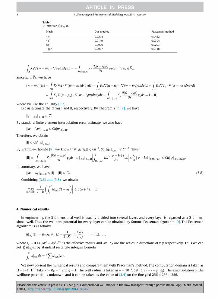
Table 1L1 error for

R cb uj@Bd

dz.

Mesh Our method Peaceman method

163 0.0274 0.0412

323 0.0149 0.0304

643 0.0076 0.0203

1283 0.0037 0.0118


Please(2014

ZX

K0rðw�whÞ � rvhdxdydz ¼ �Z

H�fa;zgK0@ðw� IhwÞ

@mvhds; 8vh 2 Vh:

Since gh 2 Vh, we have

ðw�whÞðz0Þ ¼Z

XK0rg � rðw�whÞdxdydz ¼

ZX

K0rðg � ghÞ � rðw�whÞdxdydzþZ

XK0rgh � rðw�whÞdxdydz

¼Z

XK0rðg � ghÞ � rðw� IhwÞdxdydz�

ZH�fa;zg

K0@ðw� IhwÞ

@mghds ¼ Iþ II;

where we use the equality (3.7).Let us estimate the terms I and II, respectively. By Theorem 2 in [7], we have

kg � ghk1;1;X 6 Ch:

By standard finite element interpolation error estimate, we also have

kw� Ihwk1;1;X 6 Chjwj2;1;X:

Therefore, we obtain

jIj 6 Ch2jwj2;1;X:

By Bramble–Thomée [8], we know that jghðz0Þj 6 Ch�1. So kghk0;1;X 6 Ch�1. Thus

jIIj ¼Z

H�fa;zgK0@ðw� IhwÞ

@mghds

�� 6 kghk0;1;X

ZH�fa;zg

K0@ðw� IhwÞ

@mds

�� 6 C

hkw� Ihwk0;H�fa;zg 6 Chkwk2;H�fa;zg:

In summary, we have

kw�whk0;1;X 6 jIj þ jIIj 6 Ch: ð3:8Þ

Combining (3.6) and (3.8), we obtain

maxðx;yÞ2@Bd

1c � b

Z c

buj@Bd

dz� �ah

� �� 6 Cðdþ hÞ: h

4. Numerical results

In engineering, the 3-dimensional well is usually divided into several layers and every layer is regarded as a 2-dimen-sional well. Thus the wellbore potential for every layer can be obtained by famous Peaceman algorithm [9]. The Peacemanalgorithm is as follows

uj@BdðziÞ ¼ uh x0; y0; zið Þ � 1

2pK0ln

dre

� �; i ¼ 1;2; . . . ;

where re ¼ 0:14ðDx2 þ Dy2Þ1=2 is the effective radius, and Dx; Dy are the scales in directions of x; y respectively. Thus we canget

R cb uj@Bd

dz by standard rectangle integral formula
Z c
buj@Bd

dz ¼ hX

i

uj@BdðziÞ:

We now present the numerical results and compare them with Peaceman’s method. The computation domain is taken as

X ¼ ½�1; 1�3. Take K ¼ K0 ¼ 1 and �q ¼ 1. The well radius is taken as d ¼ 10�5. Set ðb; cÞ ¼ � 120 ;

120

. The exact solution of the

wellbore potential is unknown, and it can be taken as the value of (3.4) on the fine gird 256� 256� 256.




Table 1 shows that the L1 error obtained by our method and Peaceman’s method, respectively. We observe that the con-vergence rate of our method is OðhÞ, which support our theoretical result. On the other hand, the Peaceman method does notachieve OðhÞ. Moreover, the errors of our method are much smaller than the Peaceman’s when the mesh size fixed. Thisshows the importance to develop a new method for transport problems involving well singularities.

5. Concluding remarks

In this paper, we derived the modeling error caused by the well-treatment that the well is usually treated as a line sourcein 3-dimensional case. Then we proposed a new algorithm to indicate the potential on the well boundary and analyzed thenumerical error. The numerical tests show the effectiveness and efficiency of our method.

We end this paper by remarking that the methodology and analysis presented here can be extended to the case withvariable K and finite many wells. We plan to address the convergence properties of such problems in the near future.

Acknowledgments

The author would like to thank Prof. Z.M. Chen and Prof. X.Y. Yue for their guidance and encouragement during thewriting of the paper. The author also would like to thank the anonymous referee for helpful comments.

References

[1] T. Li et al, Boundary value problems with equivalued surface boundary conditions for self-adjoint elliptic differential equations I, Fudan J. Nat. Sci. 1(1976) 61–71 (in Chinese).

[2] T. Li et al, Boundary value problems with equivalued surface boundary conditions for self-adjoint elliptic differential equations II, Fudan J. Nat. Sci. 1(1976) 136–145 (in Chinese).

[3] T. Li, A class of non-local boundary value problems for partial differential equations and its applications in numerical analysis, J. Comput. Appl. Math. 28(1998) 49–62.

[4] T. Li, Boundary value problems with equivalued surface and the resistivity well-logging, Pitman Research Notes in Mathematics Series, vol. 382,Longman, 1998.

[5] Z.M. Chen, X.Y. Yue, Numerical homogenization of well singularity in the flow transport through heterogeneous porous media, SIAM Multiscale Model.Simul. 1 (2003) 260–303.

[6] D. Gilbarg, N.S. Trudinger, Elliptic partial differential equations of second order, Classics in Mathematics, Springer-Verlag, Berlin, 2001 (Reprint of the1998 edition, pp. 94–100).

[7] R. Scott, Optimal L1estimates for the finite element method on irregular meshes, Math. Comput. 30 (1976) 681–697.[8] J.H. Bramble, V. Thomée, Pointwise bounds for discrete green function, Simul. J. Numer. Anal. 6 (4) (1969) 583–590.[9] D.W. Peaceman, Interpretation of wellblock pressure in numerical reservoir simulation, SEPJ, Trans., AIME 253, 1978, p. 183.

Please cite this article in press as: T. Zhang, A 3-dimensional well model in the flow transport through porous media, Appl. Math. Modell.(2014), http://dx.doi.org/10.1016/j.apm.2014.03.045

http://refhub.elsevier.com/S0307-904X(14)00148-6/h0005


















a 3-dimensional well model in the flow transport through porous media

Documents