7. heat / mass transfer analogy - users.abo.fi · februari 2015 Åbo akademi -kemiteknik...

RoNz

4243

02

Mas

söve

rför

ing

och

Sep

arat

ions

tekn

ik

februari 2015 Åbo Akademi - kemiteknik - Värme- och strömningsteknik Biskopsgatan 8, 20500 Åbo

1/36

Mass transfer and separation technologyMassöverföring och separationsteknik (”MÖF-ST”)

7. Heat / mass transfer analogy

Ron ZevenhovenÅbo Akademi University

Thermal and Flow Engineering Laboratorytel. 3223 ; [email protected]

RoNz

4243

02

Mas

söve

rför

ing

och

Sep

arat

ions

tekn

ik


2/36

7.1 Heat / mass transfer analogy

RoNzfebruari 2015 Åbo Akademi - kemiteknik - Värme- och strömningsteknik Biskopsgatan 8, 20500 Åbo

3/36

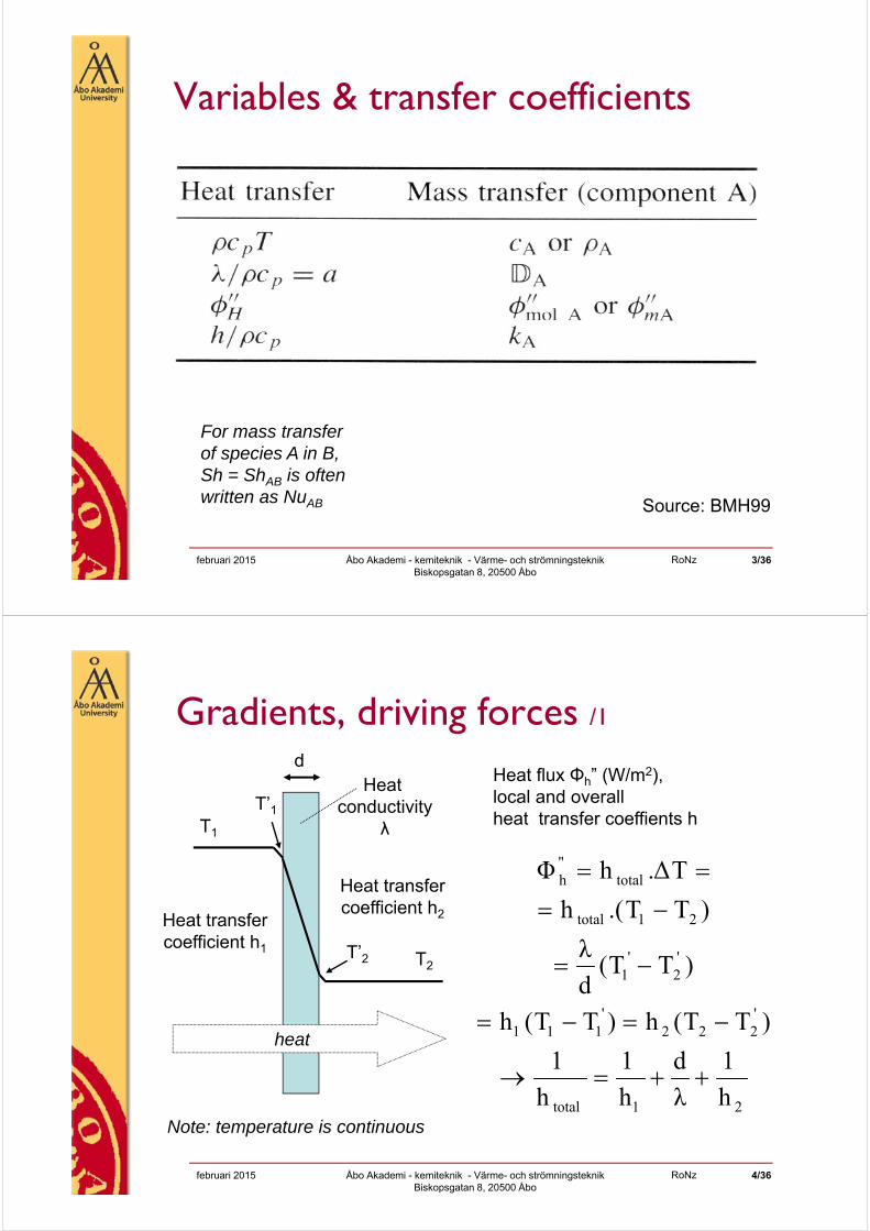
Variables & transfer coefficients

Source: BMH99

For mass transfer of species A in B, Sh = ShAB is often written as NuAB


4/36

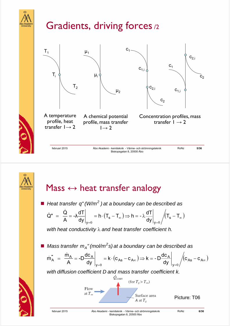
Gradients, driving forces /1

T1

T2

Heat transfercoefficient h2Heat transfer

coefficient h1

dHeat

conductivityλ

T’1

T’2

hλ

d

hh

)TT(h)TT(h

)TT(d

λ

)TT.(h

TΔ.hΦ

total

''

''

total

total"h

Heat flux Φh” (W/m2), local and overall heat transfer coeffients h

Note: temperature is continuous

heat


5/36

Gradients, driving forces /2

A temperatureprofile, heat

transfer 1→ 2

T2

Ti

T1

µ2

µi

µ1c1

c2

c1,i

c2,i

c1

c1,i

c2,i

c2

A chemical potential profile, mass transfer

1→ 2

Concentration profiles, masstransfer 1 → 2


6/36

Mass ↔ heat transfer analogy

Picture: T06

k. tcoefficien transfermass and D tcoefficien diffusion with

-

as described be can boundary a at s)(mol/m"m transferMass

h. tcoefficien transfer heat and tyconductivi heat with

-

as described be can boundary a at )(W/mq" transfer Heat

2A

2

AAsy

AAAs

y

AAA

sy

sy

ccdy

dcDkcck

dy

dc-D

A

m m

TTdydT

hTThdy

dT-λ

A

Q " Q

00

00

"


7/36

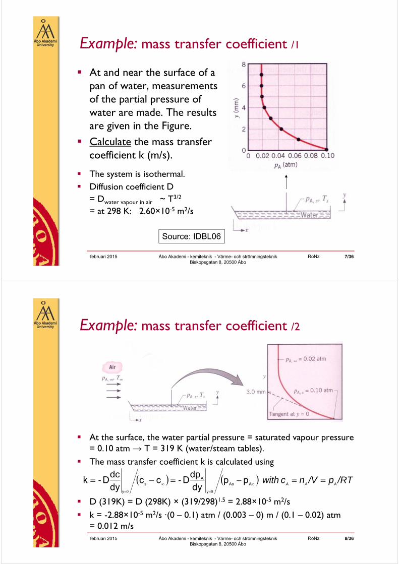
Example: mass transfer coefficient /1

At and near the surface of a pan of water, measurementsof the partial pressure of water are made. The resultsare given in the Figure.

Calculate the mass transfer coefficient k (m/s).

The system is isothermal. Diffusion coefficient D

= Dwater vapour in air ~ T3/2

= at 298 K: 2.60×10-5 m2/s

Source: IDBL06


8/36

Example: mass transfer coefficient /2

At the surface, the water partial pressure = saturated vapour pressure = 0.10 atm → T = 319 K (water/steam tables).

The mass transfer coefficient k is calculated using

D (319K) = D (298K) × (319/298)1.5 = 2.88×10-5 m2/s k = -2.88×10-5 m2/s ·(0 – 0.1) atm / (0.003 – 0) m / (0.1 – 0.02) atm

= 0.012 m/s

/RTp/Vnc with --AAA

AAs

y

As

y

ppdydp

Dccdydc

Dk


9/36

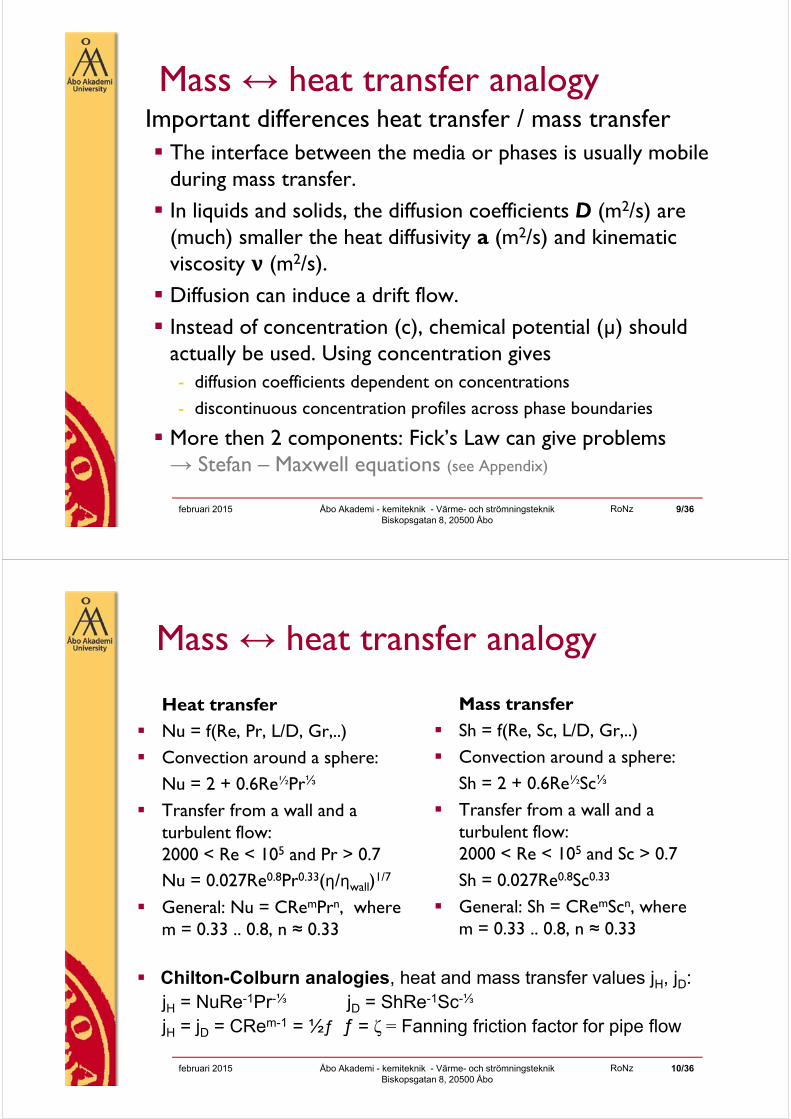
Mass ↔ heat transfer analogyImportant differences heat transfer / mass transfer The interface between the media or phases is usually mobile

during mass transfer. In liquids and solids, the diffusion coefficients D (m2/s) are

(much) smaller the heat diffusivity a (m2/s) and kinematicviscosity ν (m2/s). Diffusion can induce a drift flow. Instead of concentration (c), chemical potential (µ) should

actually be used. Using concentration gives - diffusion coefficients dependent on concentrations- discontinuous concentration profiles across phase boundaries

More then 2 components: Fick’s Law can give problems → Stefan – Maxwell equations (see Appendix)


10/36

Mass ↔ heat transfer analogy

Heat transfer Nu = f(Re, Pr, L/D, Gr,..) Convection around a sphere:

Nu = 2 + 0.6Re½Pr⅓

Transfer from a wall and a turbulent flow: 2000 < Re < 105 and Pr > 0.7Nu = 0.027Re0.8Pr0.33(η/ηwall)1/7

General: Nu = CRemPrn, wherem = 0.33 .. 0.8, n ≈ 0.33

Mass transfer Sh = f(Re, Sc, L/D, Gr,..) Convection around a sphere:

Sh = 2 + 0.6Re½Sc⅓

Transfer from a wall and a turbulent flow: 2000 < Re < 105 and Sc > 0.7Sh = 0.027Re0.8Sc0.33

General: Sh = CRemScn, wherem = 0.33 .. 0.8, n ≈ 0.33

Chilton-Colburn analogies, heat and mass transfer values jH, jD:jH = NuRe-1Pr-⅓ jD = ShRe-1Sc-⅓

jH = jD = CRem-1 = ½ƒ ƒ = ζ = Fanning friction factor for pipe flow


11/36

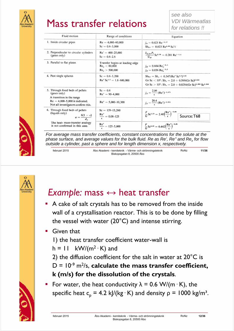
Mass transfer relations

f

Source: T68

For average mass transfer coefficients, constant concentrations for the solute at thephase surface, and average values for the bulk fluid. Re as Re’, Re’’ and Rex for flow outside a cylinder, past a sphere and for length dimension x, respectively.

see also VDI Wärmeatlas for relations !!


12/36

Example: mass ↔ heat transfer A cake of salt crystals has to be removed from the inside

wall of a crystallisation reactor. This is to be done by fillingthe vessel with water (20°C) and intense stirring.

Given that 1) the heat transfer coefficient water-wall is h = 11 kW/(m2· K) and 2) the diffusion coefficient for the salt in water at 20°C is D = 10-9 m2/s, calculate the mass transfer coefficient, k (m/s) for the dissolution of the crystals.

For water, the heat conductivity λ = 0.6 W/(m· K), the specific heat cp = 4.2 kJ/(kg· K) and density ρ = 1000 kg/m³.


13/36

Example: mass ↔ heat transfer Answer:

The Chilton-Colburn relations jH = Nu· Re-1· Pr-⅓ and jD = Sh· Re-1· Sc-⅓ give:

Sh = k· d/D = Nu· (Sc/Pr)⅓ = Nu· (a/D)⅓

with a = λ/(ρ· cp) and Nu = h· d/λ,

with characeristic size d (not needed here).

This then gives for k the expression:k = (h / (ρ· cp)⅓) · (D/λ)⅔

which gives result k = 9.6×10-5 m/s

RoNz

4243

02

Mas

söve

rför

ing

och

Sep

arat

ions

tekn

ik


14/36

7.2 Transfer coefficients and boundarylayers


15/36

Boundary layers /1

Source: MSH93Divergingchannel

Tube flow

Flat plate

Velocity V = 0.99·Vundisturbed flow


16/36

Fluid flow in a tube or otherconfinement (sv: inspärrning) will show: – zero velocity (the no-slip condition) at the

walls; and – maximum velocity furthest from the walls

(i.e. at a tube flow centre line or at a freesurface)

The velocity profile is the result of viscous friction, and for turbulent flow, ”eddy” currents (→ so-called ”eddyviscosity”: η = ηviscous + ηeddy )

In many applications a plug flow idealisation may be used described by an average velocity <v>

pict

ures

: http

://w

ww

.spi

raxs

arco

.com

/lear

n/m

odul

es/4

_1_0

1.as

p

Plug flow idealisation

Velocity profile due to viscous friction

Velocity profile due to turbulent ”eddies”

Internal flows; velocity profiles


17/36

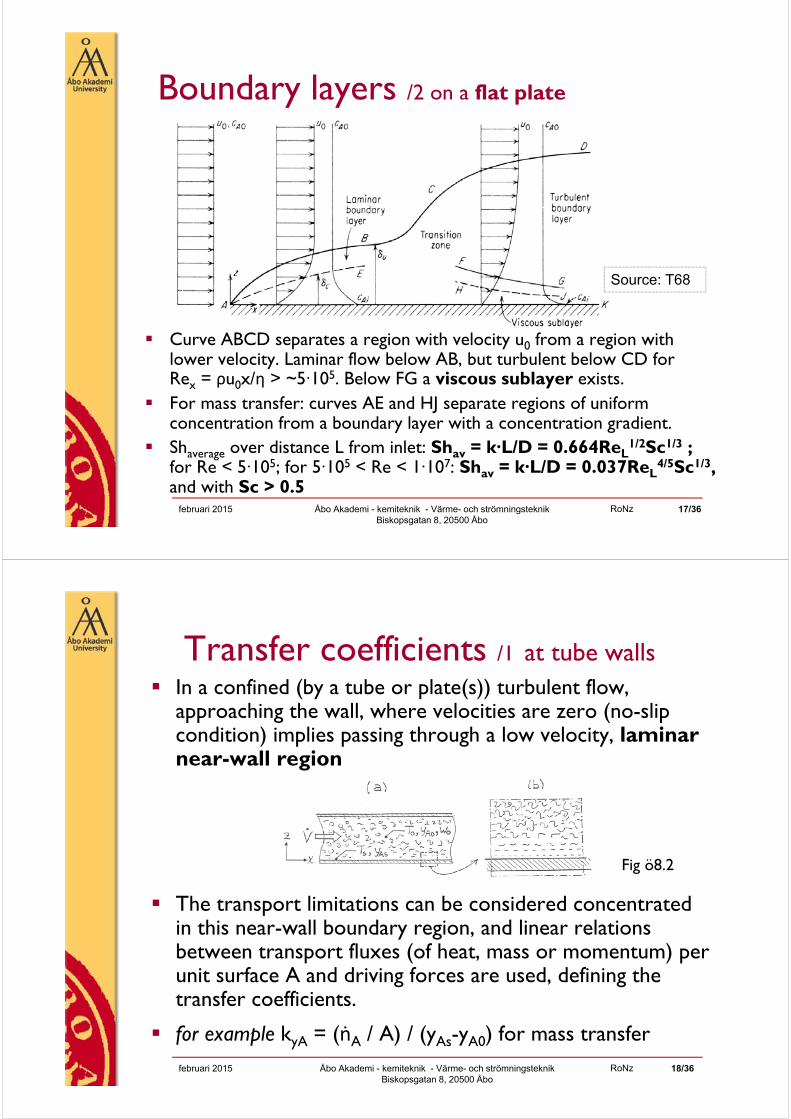
Boundary layers /2 on a flat plate

Curve ABCD separates a region with velocity u0 from a region with lower velocity. Laminar flow below AB, but turbulent below CD for Rex = ρu0x/η > ~5·105. Below FG a viscous sublayer exists.

For mass transfer: curves AE and HJ separate regions of uniform concentration from a boundary layer with a concentration gradient.

Shaverage over distance L from inlet: Shav = k·L/D = 0.664ReL1/2Sc1/3 ;

for Re < 5·105; for 5·105 < Re < 1·107: Shav = k·L/D = 0.037ReL4/5Sc1/3,

and with Sc > 0.5

Source: T68


18/36

Transfer coefficients /1 at tube walls In a confined (by a tube or plate(s)) turbulent flow,

approaching the wall, where velocities are zero (no-slipcondition) implies passing through a low velocity, laminarnear-wall region

The transport limitations can be considered concentratedin this near-wall boundary region, and linear relations between transport fluxes (of heat, mass or momentum) per unit surface A and driving forces are used, defining the transfer coefficients.

for example kyA = (ṅA / A) / (yAs-yA0) for mass transfer

Fig ö8.2


19/36

Transfer coefficients /2

Mass transfer coefficient: kyA = (ṅA / A) / (yAs-yA0) Heat transfer coefficient for heat flow Q and driving force

(Ts – T0) gives h = (Q / A)/(Ts – T0) Momentum transfer coefficient (Fanning friction factor ƒ =

ζ = Blasisus friction fractor 4ƒ) for fluid flow wall friction Fτand main stream fluidvelocity v0 gives ƒ = (Fτ /A) / (½ρv0²)

kyA, h and ƒ follow from relations between dimension- less groups Re, Nu, Sh, Pr and Sc, + several others.

Boundary layer thickness δ can be related to the diffusion coefficients D, a = λ/(ρ· cp) and v = η/ρ

The ratio between the boundary layer thicknessesintroduces Pr and Sc:

δhydrodynamic / δthermal = Pr1/3, δhydrodynamic / δmass transfer = Sc1/3

.

.


20/36

Transfer coefficients /3

For geometrically similar situations, heat ↔ mass ↔momentum transfer analogy can be used, for example for turbulent tube flow

Sh = 0.027· Re0.80· Sc1/3 Nu = 0.027· Re0.80· Pr1/3

ƒ = ζ = 0.027· Re0.80·2· Re-1

Alternatively, dividing Sh by Re· Sc⅓ , Nu by Re· Pr⅓ and f by Re gives the Chilton-Colburn analogy (or Reynolds analogy) numbers jH = jM = ½·ƒ(Fanning) = ½· ζ = constant.

The heat ↔ mass transfer analogy is very robust, but the vector nature of velocity makes momentumtransfer sensitive to flow system geometry and structure


21/36

Boundary layer models /1 The laminar boundary layer models concentrate transfer

limitations and gradients in flow situations a laminar flow layer near the confining walls. In the boundary layer, diffusion according to Laws of Fourier, Fick and Newton. This neglects the hydrodynamic correction effects of the Pr and Sc numbers: δhydrodynamic/δthermal = Pr1/3, δhydrodynamic/δmass transfer = Sc1/3

More correctly, the transport by turbulent eddies is taken into account as well.

Fig ö8.3


22/36

Boundary layer models /2

A simple approach is to assume a stagnant layer near the wall from which mass, heat or momentum is taken into the main flow by short-living turbulent eddies

For a mass flux me of these eddies, fluxes of heat, mass or momentum can be written as Q = me∙cp∙ΔT, ṅA = me∙Δy/MA and İ = meΔw

This results in Nu· Pr-1 = Sh· Sc-1 = ½·ƒ· Re No satisfying agreement with experiments and emperical

expressions exists: more theory improvement is needed.

Fig ö 8.3

.. .

. .


23/36

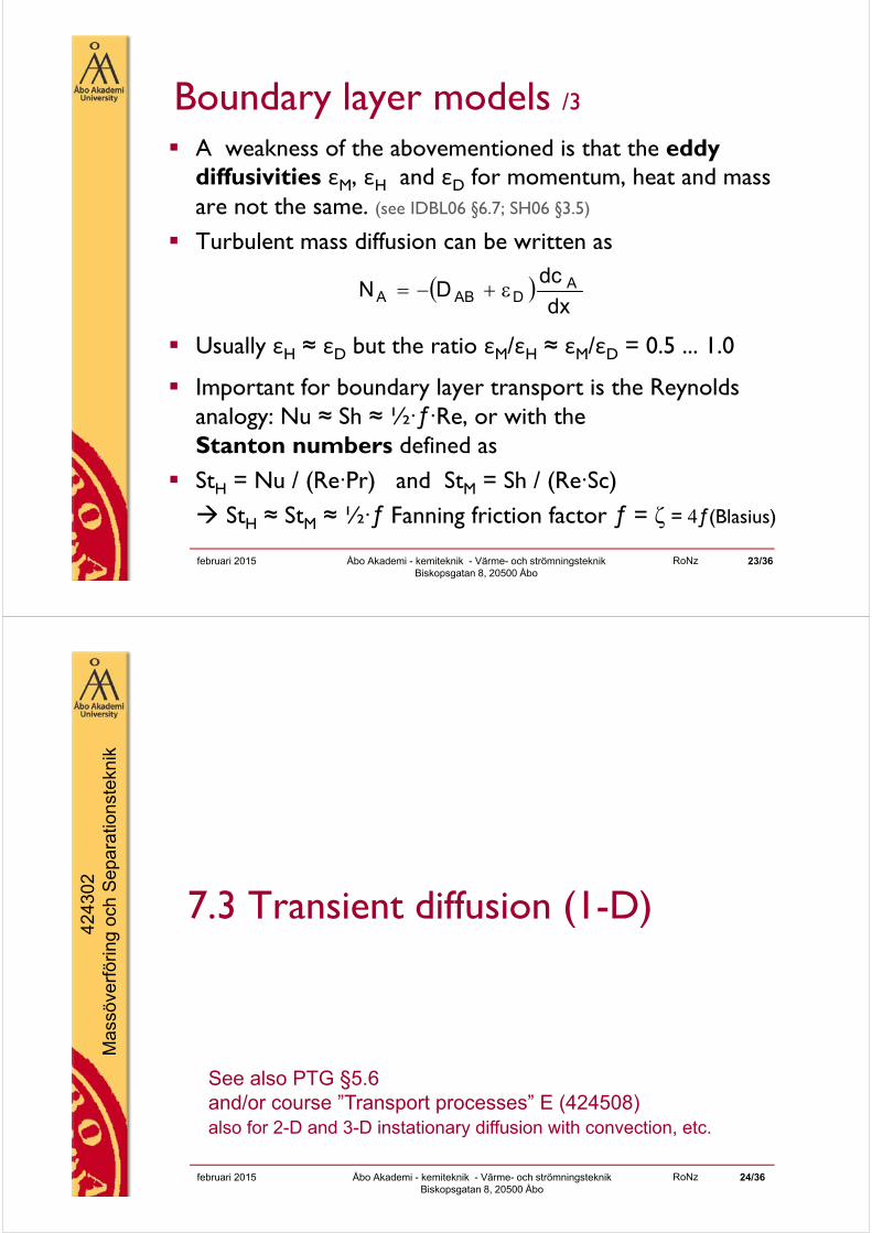
Boundary layer models /3

A weakness of the abovementioned is that the eddydiffusivities εM, εH and εD for momentum, heat and massare not the same. (see IDBL06 §6.7; SH06 §3.5)

Turbulent mass diffusion can be written as

Usually εH ≈ εD but the ratio εM/εH ≈ εM/εD = 0.5 ... 1.0

Important for boundary layer transport is the Reynolds analogy: Nu ≈ Sh ≈ ½·ƒ·Re, or with the Stanton numbers defined as

StH = Nu / (Re·Pr) and StM = Sh / (Re·Sc) StH ≈ StM ≈ ½·ƒ Fanning friction factor ƒ = ζ = 4ƒ(Blasius)

dx

dcDN A

DABA

RoNz

4243

02

Mas

söve

rför

ing

och

Sep

arat

ions

tekn

ik


24/36

7.3 Transient diffusion (1-D)

See also PTG §5.6and/or course ”Transport processes” E (424508)also for 2-D and 3-D instationary diffusion with convection, etc.


25/36

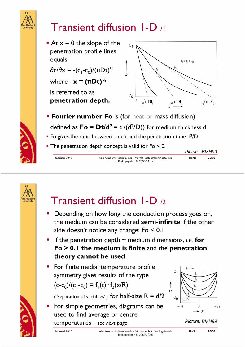
At x = 0 the slope of the penetration profile linesequals

∂c/∂x = -(c1-c0)/(πDt)½

where x = (πDt)½

is referred to as penetration depth.

Fourier number Fo is (for heat or mass diffusion)

defined as Fo = Dt/d2 = t /(d2/D)) for medium thickness d

Fo gives the ratio between time t and the penetration time d2/D

The penetration depth concept is valid for Fo < 0.1Picture: BMH99

DtπDtπDtπ

c0

c1

c

Transient diffusion 1-D /1


26/36

Transient diffusion 1-D /2

Depending on how long the conduction process goes on, the medium can be considered semi-infinite if the otherside doesn’t notice any change: Fo < 0.1

If the penetration depth ~ medium dimensions, i.e. for Fo > 0.1 the medium is finite and the penetration theory cannot be used

For finite media, temperature profilesymmetry gives results of the type(c-c0)/(c1-c0) = f1(t)· f2(x/R)

(“separation of variables”) for half-size R = d/2

For simple geometries, diagrams can be used to find average or centretemperatures – see next page Picture: BMH99

c0

c1

c


27/36

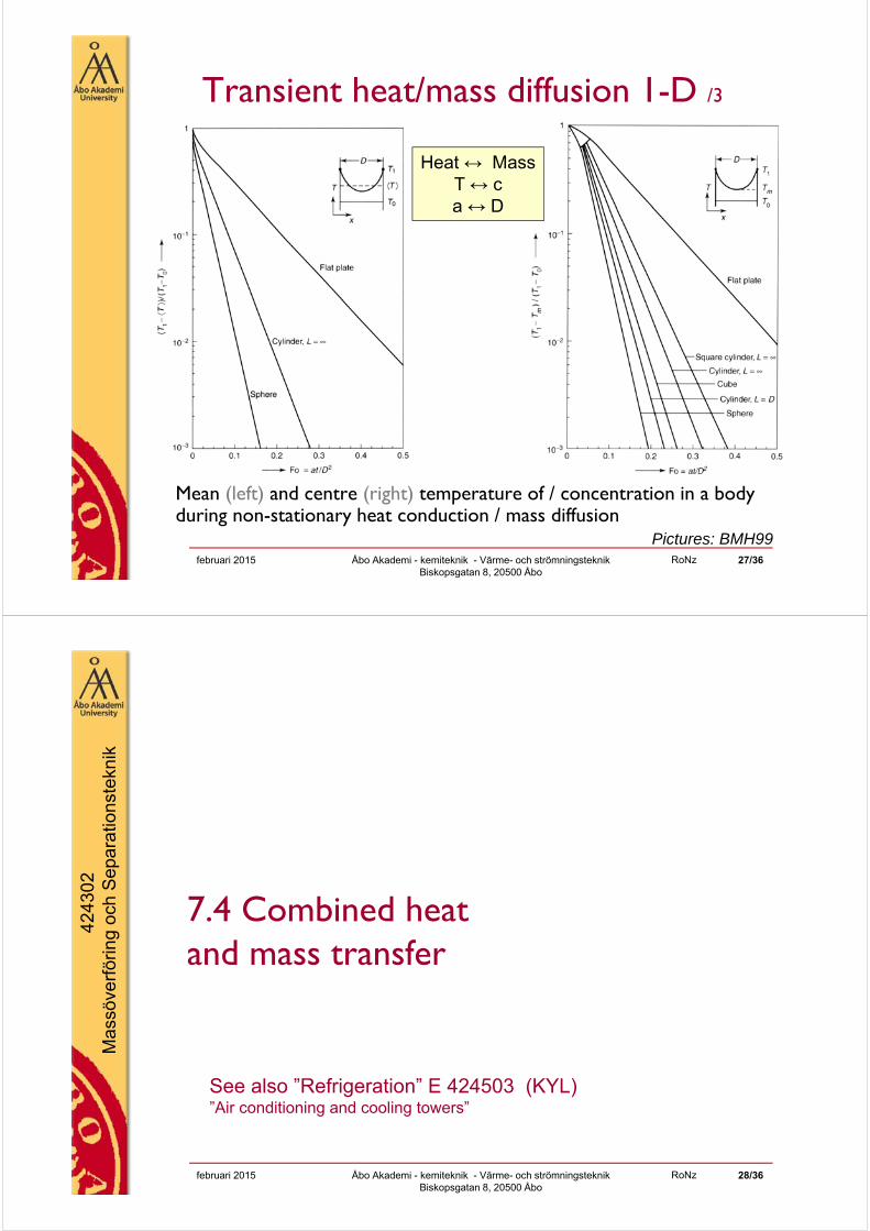
Transient heat/mass diffusion 1-D /3

Mean (left) and centre (right) temperature of / concentration in a body during non-stationary heat conduction / mass diffusion

Pictures: BMH99

Heat ↔ MassT ↔ ca ↔ D

RoNz

4243

02

Mas

söve

rför

ing

och

Sep

arat

ions

tekn

ik


28/36

7.4 Combined heat and mass transfer

See also ”Refrigeration” E 424503 (KYL)”Air conditioning and cooling towers”


29/36

Evaporation from a wet surface Steady-state evaporation of

a droplet, with heat of vaporisation ΔHvap :Φ”H = Φ”molA· ΔHvap

Φ”H = h· (Tg –Tw)Φ”molA = k· (cA,w – cA,g)

= k· (pA,w – pA,g)/(RTaverage)

This gives (pA,w – pA,g)/(Tg –Tw) = RTaverage/(ΔHvap)· h/k h/k = (Nu·λ)/(Sh· D) ≈ λ/D for a stagnant medium (Re small)

h/k = (Nu·λ)/(Sh· D) ≈ (λ/D)· (Pr/Sc)⅓ = (ρ· cp)· (Sc/Pr)⅔

(Re not small) with Sc/Pr = Le (Lewis number) = a/D Temperature Tw is known as ”wet bulb temperature”

Source: BMH99


30/36

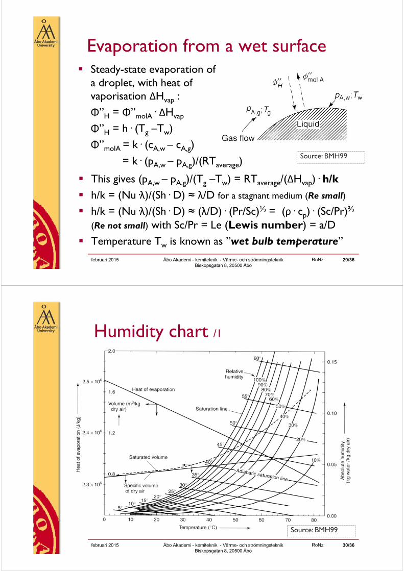
Humidity chart /1

Source: BMH99


31/36

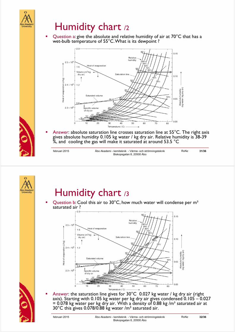
Humidity chart /2

Answer: absolute saturation line crosses saturation line at 55°C. The right axisgives absolute humidity 0.105 kg water / kg dry air. Relative humidity is 38-39 %, and cooling the gas will make it saturated at around 53.5 °C

Question a: give the absolute and relative humidity of air at 70°C that has a wet-bulb temperature of 55°C. What is its dewpoint ?


32/36

Humidity chart /3

Answer: the saturation line gives for 30°C 0.027 kg water / kg dry air (right axis). Starting with 0.105 kg water per kg dry air gives condensed 0.105 – 0.027 = 0.078 kg water per kg dry air. With a density of 0.88 kg /m³ saturated air at 30°C this gives 0.078/0.88 kg water /m3 saturated air.

Question b: Cool this air to 30°C, how much water will condense per m³ saturated air ?


33/36

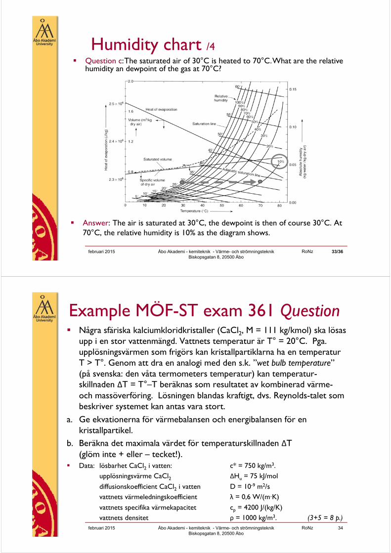
Humidity chart /4

Answer: The air is saturated at 30°C, the dewpoint is then of course 30°C. At 70°C, the relative humidity is 10% as the diagram shows.

Question c: The saturated air of 30°C is heated to 70°C. What are the relative humidity an dewpoint of the gas at 70°C?

RoNz

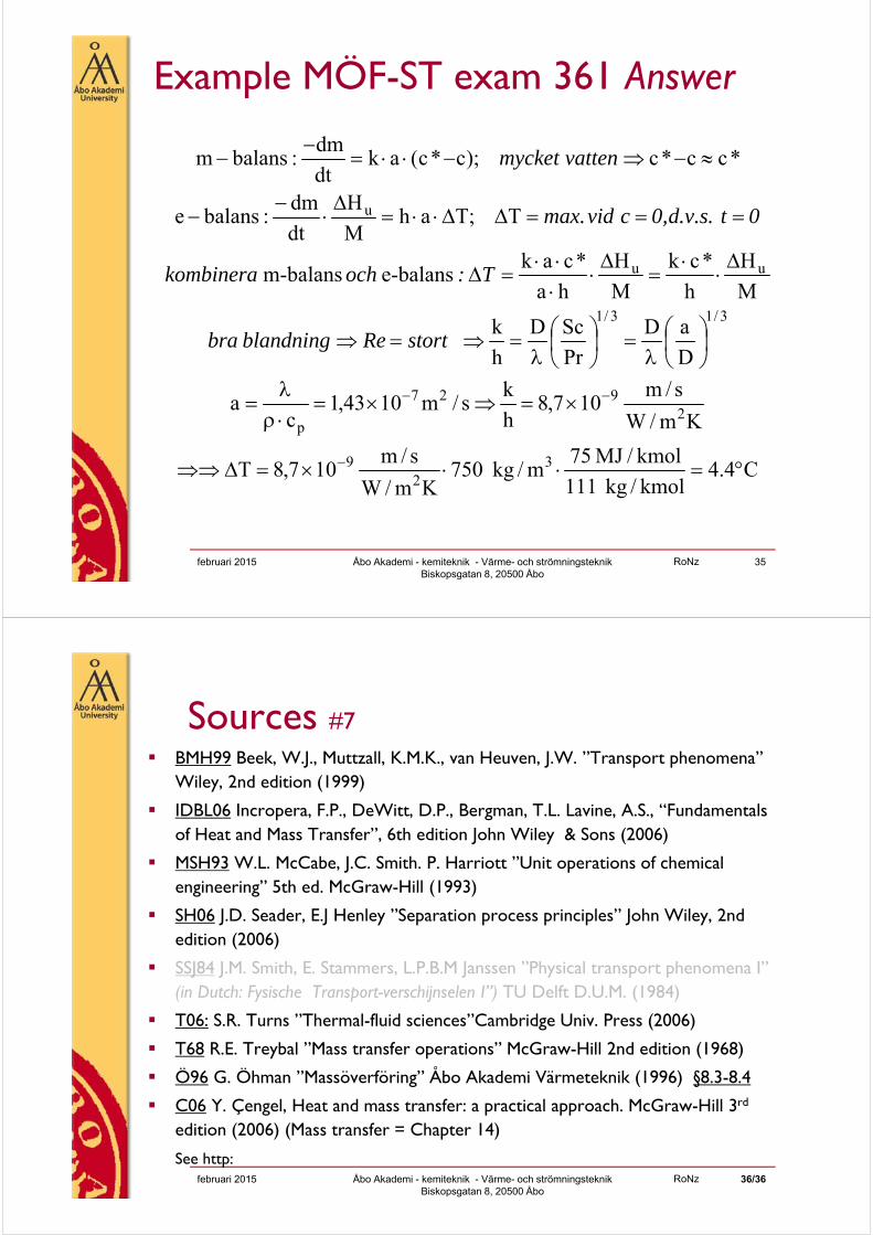
Example MÖF-ST exam 361 Question Några sfäriska kalciumkloridkristaller (CaCl2, M = 111 kg/kmol) ska lösas

upp i en stor vattenmängd. Vattnets temperatur är T° = 20°C. Pga. upplösningsvärmen som frigörs kan kristallpartiklarna ha en temperatur T > T°. Genom att dra en analogi med den s.k. ”wet bulb temperature” (på svenska: den våta termometers temperatur) kan temperatur-skillnaden ΔT = T°–T beräknas som resultatet av kombinerad värme-och massöverföring. Lösningen blandas kraftigt, dvs. Reynolds-talet som beskriver systemet kan antas vara stort.

a. Ge ekvationerna för värmebalansen och energibalansen för en kristallpartikel.

b. Beräkna det maximala värdet för temperaturskillnaden ΔT (glöm inte + eller – tecket!).

Data: lösbarhet CaCl2 i vatten: c* = 750 kg/m3.upplösningsvärme CaCl2 ΔHu = 75 kJ/mol

diffusionskoefficient CaCl2 i vatten D = 10-9 m2/svattnets värmeledningskoefficient λ = 0,6 W/(m·K)

vattnets specifika värmekapacitet cp = 4200 J/(kg/K)vattnets densitet ρ = 1000 kg/m3. (3+5 = 8 p.)


34

RoNz

Example MÖF-ST exam 361 Answer


35

C4.4kmol/kg111

kmol/MJ75m/kg750

Km/W

s/m107,8T

Km/W

s/m107,8

h

ks/m1043,1

ca

D

aD

Pr

ScD

h

k

M

H

h

*ck

M

H

ha

*cake-balansm-balans

T;TahM

H

dt

dm:balanse

*cc*c);c*c(akdt

dm:balansm

32

9

2927

p

3/13/1

uu

u

stort Reblandningbra

T: och kombinera

0t d.v.s.0,c vid max.

vatten mycket


36/36

Sources #7 BMH99 Beek, W.J., Muttzall, K.M.K., van Heuven, J.W. ”Transport phenomena”

Wiley, 2nd edition (1999)

IDBL06 Incropera, F.P., DeWitt, D.P., Bergman, T.L. Lavine, A.S., “Fundamentals of Heat and Mass Transfer”, 6th edition John Wiley & Sons (2006)

MSH93 W.L. McCabe, J.C. Smith. P. Harriott ”Unit operations of chemicalengineering” 5th ed. McGraw-Hill (1993)

SH06 J.D. Seader, E.J Henley ”Separation process principles” John Wiley, 2nd edition (2006)

SSJ84 J.M. Smith, E. Stammers, L.P.B.M Janssen ”Physical transport phenomena I” (in Dutch: Fysische Transport-verschijnselen I”) TU Delft D.U.M. (1984)

T06: S.R. Turns ”Thermal-fluid sciences”Cambridge Univ. Press (2006)

T68 R.E. Treybal ”Mass transfer operations” McGraw-Hill 2nd edition (1968)

Ö96 G. Öhman ”Massöverföring” Åbo Akademi Värmeteknik (1996) §8.3-8.4

C06 Y. Çengel, Heat and mass transfer: a practical approach. McGraw-Hill 3rd

edition (2006) (Mass transfer = Chapter 14)

See http:

7. heat / mass transfer analogy - users.abo.fi · februari 2015 Åbo akademi -kemiteknik...

Documents