7 covering, staffing & cutting stock models

115

7

Covering, Staffing & Cutting Stock Models

7.1 Introduction Covering problems tend to arise in service industries. The crucial feature is that there is a set of

requirements to be covered. We have available to us various activities, each of which helps cover some,

but not all, the requirements. The qualitative form of a covering problem is:

Choose a minimum cost set of activities

Subject to

The chosen activities cover all of our requirements.

Some examples of activities and requirement types for various problems are listed below:

Problem Requirements Activities

Staff scheduling Number of people

required on duty

each period of the

day or week.

Work or shift patterns. Each

pattern covers some, but not all,

periods.

Routing Each customer

must be visited.

Various feasible trips, each of

which covers some, but not all,

customers.

Cutting of bulk

raw material

stock (e.g., paper,

wood, steel,

textiles)

Units required of

each finished

good size.

Cutting patterns for cutting raw

material into various finished

good sizes. Each pattern

produces some, but not every,

finished good.

In the next sections, we look at several of these problems in more detail.

116 Chapter 7 Covering, Staffing & Cutting Stock

7.1.1 Staffing Problems One part of the management of most service facilities is the scheduling or staffing of personnel. That is,

deciding how many people to use on what shifts. This problem exists in staffing the information

operators department of a telephone company, a toll plaza, a large hospital, and, in general, any facility

that must provide service to the public.

The solution process consists of at least three parts: (1) Develop good forecasts of the number of

personnel required during each hour of the day or each day of the week during the scheduling period.

(2) Identify the possible shift patterns, which can be worked based on the personnel available and work

agreements and regulations. A particular shift pattern might be to work Tuesday through Saturday and

then be off two days. (3) Determine how many people should work each shift pattern, so costs are

minimized and the total number of people on duty during each time period satisfies the requirements

determined in (1). All three of these steps are difficult. LP can help in solving step 3.

One of the first published accounts of using optimization for staff scheduling was by Edie (1954).

He developed a method for staffing tollbooths for the New York Port Authority. Though old, Edie’s

discussion is still very pertinent and thorough. His thoroughness is illustrated by his summary (p. 138):

“A trial was conducted at the Lincoln Tunnel...Each toll collector was given a slip showing his booth

assignments and relief periods and instructed to follow the schedule strictly...At no times did excessive

backups occur...The movement of collectors and the opening and closing of booths took place without

the attention of the toll sergeant. At times, the number of booths were slightly excessive, but not to the

extent previously... Needless to say, there is a good deal of satisfaction...”

7.1.2 Example: Northeast Tollway Staffing Problems The Northeast Tollway out of Chicago has a toll plaza with the following staffing demands during each

24-hour period:

Hours

Collectors Needed

12 A.M. to 6 A.M. 2

6 A.M. to 10 A.M. 8

10 A.M. to Noon 4

Noon to 4 P.M. 3

4 P.M. to 6 P.M. 6

6 P.M. to 10 P.M. 5

10 P.M. to 12 Midnight 3

Each collector works four hours, is off one hour, and then works another four hours. A collector can

be started at any hour. Assuming the objective is to minimize the number of collectors hired, how many

collectors should start work each hour?

Formulation and Solution Define the decision variables:

x1 = number of collectors to start work at 12 midnight,

x2 = number of collectors to start work at 1 A.M., .

.

. x24 = number of collectors to start work at 11 P.M.

Covering, Staffing & Cutting Stock Chapter 7 117

There will be one constraint for each hour of the day, which states the number of collectors on at

that hour be the number required for that hour. The objective will be to minimize the number of collectors

hired for the 24-hour period. More formally:

Minimize x1 + x2 + x3 + ... + x24

subject to

x1 + x24 + x23 + x22 + x20 + x19 + x18 + x17 2 (12 midnight to 1 A.M.).

x2 + x1 + x24 + x23 + x21 + x20 + x19 + x18 2 (1 A.M. to 2 A.M.) .

.

.

x7 + x6 + x5 + x4 + x2 + x1 + x24 + x23 8 (6 A.M. to 7 A.M.) .

.

.

x24 + x23 + x22 + x21 + x19 + x18 + x17 + x16 3 (11 P.M. to 12 midnight)

It may help to see the effect of the one hour off in the middle of the shift by looking at the

“PICTURE” of equation coefficients:

Constraint Row x1 x2 x3 x4 x5 x6 x7 x8 x9 ... x17 x18 x19 x20 x21 x22 x23 x24 RHS

12 A.M. to 1 A.M. 1 1 1 1 1 1 1 1 2

1 A.M. to 2 A.M. 1 1 1 1 1 1 1 1 1 2

2 A.M. to 3 A.M. 1 1 1 1 1 1 1 1 2

3 A.M. to 4 A.M. 1 1 1 1 1 1 1 1 2

4 A.M. to 5 A.M. 1 1 1 1 1 1 1 1 2

5 A.M. to 6 A.M. 1 1 1 1 1 1 1 1 2

6 A. M. to 7 A.M. 1 1 1 1 1 1 1 1 8

7 A.M. to 8 A.M. 1 1 1 1 1 1 1 1 8

8 A.M. to 9 A.M. 1 1 1 1 1 1 1 1 8

9 A.M. to 10 A.M. 1 1 1 1 1 1 1 8

10 A.M. to 11 A.M. 1 1 1 1 1 1 4

11 A.M. to 12 P.M. 1 1 1 1 1 4

12 P.M. to 1 P.M. 1 1 1 1 3

1 P.M. to 2 P.M. 1 1 1 1 3

2 P.M. to 3 P.M. 1 1 1 3

etc. etc.


Sets Based Formulation

A “sets” based formulation for this problem in LINGO is quite compact. There are two sets, one for the

24-hour day and the other for the nine-hour shift. Note the use of the @WRAP function to modulate the

index for the X variable:

MODEL: ! 24 hour shift scheduling;

SETS: !Each shift is4 hours on, 1 hour off, 4 hours on;

HOUR/1..24/: X, NEED;

ENDSETS

DATA:

NEED=2 2 2 2 2 2 8 8 8 8 4 4 3 3 3 3 6 6 5 5 5 5 3 3;

ENDDATA

MIN = @SUM( HOUR(I): X(I));

@FOR( HOUR( I): ! People on duty in hour I are those who

started 9 or less hours earlier, but not 5;

@SUM(HOUR(J)|(J#LE#9)#AND#(J#NE#5): X(@WRAP((I-J+1),24)))>= NEED(I));

END

When solved as an LP, we get an objective value of 15.75 with the following variables nonzero:

x2 = 5 x5 = 0.75 x11 = 1 x16 = 1

x3 = 0.75 x6 = 0.75 x14 = 1 x17 = 1

x4 = 0.75 x7 = 0.75 x15 = 2 x18 = 1

The answer is not directly useful because some of the numbers are fractional. To enforce the

integrality restriction, use the @GIN function as in the following line:

@FOR( HOUR(I): @GIN( X(I)));

When it is solved, we get an objective value of 16 with the following variables nonzero:

x2 = 4 x5 = 1 x14 = 1 x17 = 2

x3 = 1 x6 = 1 x15 = 1 x18 = 1

x4 = 1 x7 = 1 x16 = 2

One of the biggest current instances of this kind of staffing problem is in telephone call centers.

Examples are telephone order takers for catalog retailers and credit checkers at credit card service

centers. A significant fraction of the population of Omaha, Nebraska works in telephone call centers. A

typical shift pattern at a call center consists of 8 hours of work split by a 15 minute break, a half hour

lunch break, and another 15 minute break.

7.1.3 Additional Staff Scheduling Features In a complete implementation there may be a fourth step, rostering, in addition to the first three steps

of forecasting, work pattern identification, and work pattern selection. In rostering, specific individuals

by name are assigned to specific work patterns. In some industries, e.g., airlines, individuals(e.g.,

pilots) are allowed to bid on the work patterns that have been selected.

In some staffing situations, there may be multiple skill requirements that need to be covered, e.g.

during the first hour there must be at least 3 Spanish speakers on duty and at least 4 English speakers.

Different employees may have different sets of skills, e.g., some may speak only English, some are

conversant in both English and Spanish, etc.


In some situations, e.g., mail processing, demand may be postponeable by one or two periods, so

that we are allowed to be understaffed, say during a peak period, if the carryover demand can be

processed in the next period.

In almost all situations, demand is somewhat random so that staff requirements are somewhat soft.

We might say that we need at least ten people on duty during a certain period, however, if we have

eleven on duty, the extra person will probably not be standing around idle during the full period. There

is a good chance that by chance demand will be higher than the point forecast so that we can use the

extra person. The queueing theory methods of chapter 18 are frequently used to provide estimates of

the marginal benefit of each unit of overstaffing.

7.2 Cutting Stock and Pattern Selection In industries such as paper, plastic food wrap, metal bars, and textiles, products are manufactured in

large economically produced sizes at the outset. These sizes are cut into a variety of smaller, more usable

sizes as the product nears the consumer. The determination of how to cut the larger sizes into smaller

sizes at minimal cost is known as the cutting stock problem. As an example of the so-called

one-dimensional cutting stock problem, suppose machine design dictates material is manufactured in

72-inch widths. There are a variety of ways of cutting these smaller widths from the 72-inch width, two

of which are shown in Figure 7.1.

Figure 7.1 Example Cutting Patterns

Pattern 1 Pattern 2

35

18

35

18

35

Pattern 1 has 2 inches of edge waste (72 − 2 35 = 2), whereas there is only 1 inch of edge waste

(72 − 2 18 − 35 = 1) with pattern 2. Pattern 2, however, is not very useful unless the number of linear

feet of 18-inch material required is about twice the number of linear feet of 35-inch material required.

Thus, a compromise must be struck between edge waste and end waste.

The solution of a cutting stock problem can be partitioned into the 3-step procedure discussed earlier:

(1) Forecast the needs for the final widths. (2) Construct a large collection of possible patterns for cutting

the large manufactured width(s) into the smaller widths. (3) Determine how much of each pattern should

be run of each pattern in (2), so the requirements in (1) are satisfied at minimum cost. Optimization can be

used in performing step (3).


Many large paper manufacturing firms have LP-based procedures for solving the cutting stock

problem. Actual cutting stock problems may involve a variety of cost factors in addition to the edge

waste/end waste compromise. The usefulness of the LP-based procedure depends upon the importance of

these other factors. The following example illustrates the fundamental features of the cutting stock problem

with no complicating cost factors.

7.2.1 Example: Cooldot Cutting Stock Problem The Cooldot Appliance Company produces a wide range of large household appliances such as

refrigerators and stoves. A significant portion of the raw material cost is due to the purchase of sheet

steel. Currently, sheet steel is purchased in coils in three different widths: 72 inches, 48 inches, and 36

inches. In the manufacturing process, eight different widths of sheet steel are required: 60, 56, 42, 38,

34, 24, 15, and 10 inches. All uses require the same quality and thickness of steel.

A continuing problem is trim waste. For example, one way of cutting a 72-inch width coil is to slit

it into one 38-inch width coil and two 15-inch width coils. There will then be a 4-inch coil of trim waste

that must be scrapped.

The prices per linear foot of the three different raw material widths are 15 cents for the 36-inch

width, 19 cents for the 48-inch width, and 28 cents for the 72-inch width. Simple arithmetic reveals the

costs per inch foot of the three widths are 15/36 = 0.416667 cents/(inch foot), 0.395833 cents/(inch

foot), and 0.388889 cents/(inch foot) for the 36", 48", and 72" widths, respectively.

The coils may be slit in any feasible solution. The possible cutting patterns for efficiently slitting

the three raw material widths are tabulated below.

For example, pattern C4 corresponds to cutting a 72-inch width coil into one 24-inch width and four

10-inch widths with 8 inches left over as trim waste.

The lengths of the various widths required in this planning period are:

Width 60” 56” 42” 38” 34” 24” 15” 10”

Number of feet

required 500 400 300 450 350 100 800 1000

The raw material availabilities this planning period are 1600 ft. of the 72-inch coils and 10,000 ft.

each of the 48-inch and 36-inch widths.

How many feet of each pattern should be cut to minimize costs while satisfying the requirements of

the various widths? Can you predict beforehand the amount of 36-inch material used?


7.2.2 Formulation and Solution of Cooldot Let the symbols A1, A2, . . . , E4 appearing in the following table denote the number of feet to cut of the

corresponding pattern:

Cutting Patterns for Raw Material

Number to Cut of the Required Width

Pattern 60” 56” 42” 38” 34” 24” 15” 10” Waste in

Designation 72-Inch Raw Material Inches

A1 1 0 0 0 0 0 0 1 2

A2 0 1 0 0 0 0 1 0 1

A3 0 1 0 0 0 0 0 1 6

A4 0 0 1 0 0 1 0 0 6

A5 0 0 1 0 0 0 2 0 0

A6 0 0 1 0 0 0 1 1 5

A7 0 0 1 0 0 0 0 3 0

A8 0 0 0 1 1 0 0 0 0

A9 0 0 0 1 0 1 0 1 0

B0 0 0 0 1 0 0 2 0 4

B1 0 0 0 1 0 0 1 1 9

B2 0 0 0 1 0 0 0 3 4

B3 0 0 0 0 2 0 0 0 4

B4 0 0 0 0 1 1 0 1 4

B5 0 0 0 0 1 0 2 0 8

B6 0 0 0 0 1 0 1 2 3

B7 0 0 0 0 1 0 0 3 8

B8 0 0 0 0 0 3 0 0 0

B9 0 0 0 0 0 2 1 0 9

C0 0 0 0 0 0 2 0 2 4

C1 0 0 0 0 0 1 3 0 3

C2 0 0 0 0 0 1 2 1 8

C3 0 0 0 0 0 1 1 3 3

C4 0 0 0 0 0 1 0 4 8

C5 0 0 0 0 0 0 4 1 2

C6 0 0 0 0 0 0 3 2 7

C7 0 0 0 0 0 0 2 4 2

C8 0 0 0 0 0 0 1 5 7

C9 0 0 0 0 0 0 0 7 2


48-Inch Raw Material

D0 0 0 1 0 0 0 0 0 6

D1 0 0 0 1 0 0 0 1 0

D2 0 0 0 0 1 0 0 1 4

D3 0 0 0 0 0 2 0 0 0

D4 0 0 0 0 0 1 1 0 9

D5 0 0 0 0 0 1 0 2 4

D6 0 0 0 0 0 0 3 0 3

D7 0 0 0 0 0 0 2 1 8

D8 0 0 0 0 0 0 1 3 3

D9 0 0 0 0 0 0 0 4 8

36-Inch Raw Material

E0 0 0 0 0 1 0 0 0 2

E1 0 0 0 0 0 1 0 1 2

E2 0 0 0 0 0 0 2 0 6

E3 0 0 0 0 0 0 1 2 1

E4 0 0 0 0 0 0 0 3 6

For accounting purposes, it is useful to additionally define:

T1 = number of feet cut of 72-inch patterns,



W1 = inch feet of trim waste from 72-inch patterns,



X1 = number of excess feet cut of the 60-inch width,

X2 = number of excess feet cut of the 56-inch width, .

.

.

X8 = number of excess feet cut of the 10-inch width.

It may not be immediately clear what the objective function should be. One might be tempted to

calculate a cost of trim waste per foot for each pattern cut and then minimize the total trim waste cost.

For example:

MIN = 0.3888891W1 + 0.395833W2 + 0.416667W3;

However, such an objective can easily lead to solutions with very little trim waste, but very high

cost. This is possible in particular when the cost per square inch is not the same for all raw material

widths. A more reasonable objective is to minimize the total cost. That is:

MIN = 28 * T1 + 19 * T2 + 15 * T3;


Incorporating this objective into the model, we have:

MODEL:

SETS:

! Each raw material has a Raw material width, Total used,

Waste total, Cost per unit, Waste cost, and Supply available;

RM: RWDTH,T, W, C, WCOST, S;

! Each Finished good has a Width, units Required. eXtra produced;

FG: FWDTH, REQ, X;

PATTERN: USERM, WASTE, AMT;

PXF( PATTERN, FG): NUM;

ENDSETS

DATA:

! The raw material widths;

RM = R72 R48 R36;

RWDTH= 72 48 36;

C = .28 .19 .15;

WCOST= .00388889 .00395833 .00416667;

S = 1600 10000 10000;

! The finished good widths;

FG = F60 F56 F42 F38 F34 F24 F15 F10;

FWDTH= 60 56 42 38 34 24 15 10;

REQ= 500 400 300 450 350 100 800 1000;

! Index of R.M. that each pattern uses;

USERM = 1 1 1 1 1 1 1 1 1 1

1 1 1 1 1 1 1 1 1 1

1 1 1 1 1 1 1 1 1

2 2 2 2 2 2 2 2 2 2

3 3 3 3 3;

! How many of each F.G. are in each R.M. pattern;

NUM= 1 0 0 0 0 0 0 1

0 1 0 0 0 0 1 0

0 1 0 0 0 0 0 1

0 0 1 0 0 1 0 0

0 0 1 0 0 0 2 0

0 0 1 0 0 0 1 1

0 0 1 0 0 0 0 3

0 0 0 1 1 0 0 0

0 0 0 1 0 1 0 1

0 0 0 1 0 0 2 0

0 0 0 1 0 0 1 1

0 0 0 1 0 0 0 3

0 0 0 0 2 0 0 0

0 0 0 0 1 1 0 1

0 0 0 0 1 0 2 0

0 0 0 0 1 0 1 2

0 0 0 0 1 0 0 3

0 0 0 0 0 3 0 0

0 0 0 0 0 2 1 0

0 0 0 0 0 2 0 2

0 0 0 0 0 1 3 0

0 0 0 0 0 1 2 1

0 0 0 0 0 1 1 3

0 0 0 0 0 1 0 4


0 0 0 0 0 0 4 1

0 0 0 0 0 0 3 2

0 0 0 0 0 0 2 4

0 0 0 0 0 0 1 5

0 0 0 0 0 0 0 7

0 0 1 0 0 0 0 0

0 0 0 1 0 0 0 1

0 0 0 0 1 0 0 1

0 0 0 0 0 2 0 0

0 0 0 0 0 1 1 0

0 0 0 0 0 1 0 2

0 0 0 0 0 0 3 0

0 0 0 0 0 0 2 1

0 0 0 0 0 0 1 3

0 0 0 0 0 0 0 4

0 0 0 0 1 0 0 0

0 0 0 0 0 1 0 1

0 0 0 0 0 0 2 0

0 0 0 0 0 0 1 2

0 0 0 0 0 0 0 3;

ENDDATA

! Minimize cost of raw material used;

MIN = TCOST;

TCOST = @SUM(RM(I): C(I)*T(I) );

! Compute total cost of waste;

TOTWASTE = @SUM( RM(I): WCOST(I)*W(I) );

@FOR( RM( I):

T( I) = @SUM( PATTERN( K)| USERM(K) #EQ# I: AMT( K));

! Raw material supply constraints;

T(I) <= S(I);

);

! Must produce at least amount required of each F.G.;

@FOR( FG(J):

@SUM(PATTERN(K): NUM(K,J)*AMT(K)) = REQ(J) + X(J);

);

! Turn this on to get integer solutions;

!@FOR( PATTERN(K): @GIN(AMT(K)));

! Waste related computations;

! Compute waste associated with each pattern;

@FOR( PATTERN(K):

WASTE(K) = RWDTH(USERM(K)) - @SUM(FG(J): FWDTH(J)*NUM(K,J));

);

! Waste for each R.M. in this solution;

@FOR( RM( I):

W(I) = @SUM( PATTERN( K)| USERM(K) #EQ# I: WASTE(K)*AMT( K));

);

END


If you minimize cost of waste, then you will get a different solution than if you minimize total cost

of raw materials. Two different solutions obtained under the two different objectives are compared in

the following table:

Cutting Stock Solutions

Nonzero Patterns

Trim Waste Minimizing Solution

Feet to Cut

Total Cost Minimizing Solution

Feet to Cut

A1 500 500

A2 400 400

A5 200 171.4286

A7 100 128.5714

A8 350 350

A9 50 3.571429

B8 0 32.14286

C9 0 14.28571

D1 150 96.42857

D3 25 0

Trim Waste Cost $5.44 $5.55

Total Cost $2348.00 $466.32

X4 100.000 0

X6 19650 0

T1 1600 1600

T2 10000 96.429

T3 0 0

The key difference in the solutions is the “Min trim waste” solution uses more of the 48" width raw

material, patterns D1 and D3, and cuts in a way so the edge waste is minimized. The “Min trim waste”

solution produces more of the 38” width, 550 units, than is needed, 450 units, because the objective

function does not count this as waste. The “Min trim waste” formulation has a number of alternate

optimal solutions, some having a raw material cost less than $2348. A key observation from this

example is that you should always remember your overall objective, e.g., minimize total cost or

maximize total profit, and not get distracted by optimizing secondary criteria.

Both solutions involve fractional answers. By turning on the @GIN declaration you can get an

integer answer. The cost of the “cost minimizing” solution increases to $466.34.

7.2.3 Generalizations of the Cutting Stock Problem In large cutting stock problems, it may be unrealistic to generate all possible patterns. There is an

efficient method for generating only the patterns that have a very high probability of appearing in the

optimal solution. It is beyond the scope of this section to discuss this procedure. However, it does become

important in large problems. See Chapter 18 for details. Dyckhoff (1981) describes another formulation


that avoids the need to generate patterns. However, that formulation may have a very large number of

rows.

Complications

In complex cutting stock problems, the following additional cost considerations may be important:

1. Fixed cost of setting up a particular pattern. This cost consists of lost machine time, labor,

etc. This motivates solutions with few patterns.

2. Value of overage or end waste. For example, there may be some demand next period for

the excess cut this period.

3. Underage cost. In some industries, you may supply plus or minus, say 5%, of a specified

quantity. The cost of producing the least allowable amount is measured in foregone profits.

4. Machine usage cost. The cost of operating a machine is usually fairly independent of the

material being run. This motivates solutions that cut up wide raw material widths.

5. Material specific products. It may be impossible to run two different products in the same

pattern if they require different materials (e.g., different thickness, quality, surface finish

or type).

6. Upgrading costs. It may be possible to reduce setup, edge-waste, and end-waste costs by

substituting a higher-grade material than required for a particular demand width.

7. Order splitting costs. If a demand width is produced from several patterns, then there will

be consolidation costs due to bringing the different lots of the output together for shipment.

8. Stock width change costs. A setup involving only a pattern change usually takes less time

than one involving both a pattern change and a raw material width change. This motivates

solutions that use few raw material widths.

9. Minimum and maximum allowable edge waste. For some materials, a very narrow ribbon

of edge waste may be very difficult to handle. Therefore, one may wish to restrict attention

to patterns that have either zero edge waste or edge waste that exceeds some minimum,

such as two centimeters. On the other hand, one may also wish to specify a maximum

allowable edge waste. For example, in the paper industry, edge waste may be blown down

a recycling chute. Edge waste wider than a certain minimum may be too difficult to blow

down this chute.

10. Due dates and sequencing. Some of the demands need to be satisfied immediately, whereas

others are less urgent. The patterns containing the urgent or high priority products should

be run first. If the urgent demands appear in the same patterns as low priority demands,

then it is more difficult to satisfy the high priority demands quickly.

11. Inventory restrictions. Typically, a customer’s order will not be shipped until all the

demands for the customer can be shipped. Thus, one is motivated to distribute a given

customer’s demands over as few patterns as possible. If every customer has product in

every pattern, then no customer’s order can be shipped until every pattern has been run.

Thus, there will be substantial work in process inventory until all patterns have been run.

12. Limit on 1-set patterns. In some industries, such as paper, there is no explicit cost

associated with setting up a pattern, but there is a limit on the rate at which pattern changes

can be made. It may take about 15 minutes to do a pattern change, much of this work being

done off-line without shutting down the main machine. The run time to produce one roll

set might take 10 minutes. Thus, if too many 1-set patterns are run, the main machine will

have to wait for pattern changes to be completed.


13. Pattern restrictions. In some applications, there may be a limit on the total number of final

product widths that may appear in a pattern, and/or a limit on the number of “small” widths

in a pattern. The first restriction would apply, for example, if there were a limited number

of take-up reels for winding the slit goods. The second restriction might occur in the paper

industry where rolls of narrow product width have a tendency to fall over, so one does not

want to have too many of them to handle in a single pattern. Some demanding customers

may request their product be cut from a particular position (e.g., the center) of a pattern,

because they feel the quality of the material is higher in that position.

14. Pattern pairing. In some plastic wrap manufacturing, the production process, by its nature,

produces two widths of raw material simultaneously, an upper output and a lower output.

Thus, it is essentially unavoidable that one must run the same number of feet of whatever

pattern is being used on the upper output as on the lower output. A similar situation

sometimes happens by accident in paper manufacturing. If a defect develops on the

“production belt”, a small width of paper in the interior of the width is unusable. Thus, the

machine effectively produces two output widths, one to the left of the defect, the other to

the right of the defect.

15. Bundle size and/or minimum purchase quantity. In some markets you may be forced to buy

product in bundles of a given size, e.g., 10 pieces per bundle. Further, you may be forced

to make cuts in bundles rather than in individual pieces. Thus, even though you have a

demand of 15 units for some finished good, you are forced to cut at least 20 units because

the bundle size is 10.

16. Saw thickness/kerf. If the material is sawed rather than sheared, each saw cut may remove

a small amount of material, sometimes called the kerf. Precise solution of a cutting stock

problem should take into account material lost to the kerf. Suppose the kerf is 2 mm. You

can represent the effect of kerf by adding 2 mm to each final product width and 2 mm to

each raw material width.

17. Max “smalls’ per pattern. There may be a limit on the number of “small” widths in a

pattern. This restriction might be encountered in the paper industry where rolls of narrow

product width have a tendency to tip over, so one does not want to have too many of them

to handle in a single pattern.

Most of the above complications can be incorporated by making modest changes to the pattern

generating procedure. The most troublesome complications are high fixed setup costs, order-splitting

costs, and stock width change costs. If they are important, then one will usually be forced to use some

ad hoc, manual solution procedure. An LP solution may provide some insight into which solutions are

likely to be good, but other methods must be used to determine a final workable solution.

7.2.4 Two-Dimensional Cutting Stock Problems The one-dimensional cutting stock problem is concerned with the cutting of a raw material that is in

coils. The basic idea still applies if the raw material comes in sheets and the problem is to cut these

sheets into smaller sheets. For example, suppose plywood is supplied in 48- by 96-inch rectangular

sheets and the end product demand is for sheets with dimensions in inches of 36 50, 24 36, 20 60,

and 18 30. Once you have enumerated all possible patterns for cutting a 48 96 sheet into

combinations of the four smaller sheets, then the problem is exactly as before.

Enumerating all possible two-dimensional patterns may be complicated. Two features of practical

two-dimensional cutting problems affect the difficulty of this task: (a) orientation requirements, and (b)


“guillotine” cut requirements. Applications in which (a) is important are in the cutting of wood and

fabric. For reasons of strength or appearance, a demand unit may be limited in how it is positioned on

the raw material (Imagine a plaid suit for which the manufacturer randomly oriented the pattern on the

raw material). Any good baseball player knows the grain of the bat must face the ball when hitting.

Attention must be paid to the grain of the wood if the resulting wood product is to be used for structural

or aesthetic purposes. Glass is an example of a raw material for which orientation is not important.

A pattern is said to be cuttable with guillotine cuts if each cut must be made by a shear across the full

width of the item being cut. As an example, suppose you wish to cut as many 4x5 rectangles as possible

from a 9x9 square. If you are allowed to make any kind of cut and rotation is allowed, then you can cut

4 such rectangles. If only guillotine cuts are allowed, then at most three pieces can be cut. Figure 7.2

illustrates.

Figure 7.2 Guillotine and Non-Guillotine Cuts of 4x5 from 9x9

Non-Guillotine Guillotine

7.2.5 Paper Converting: A Rectangle Cutting Problem A particular form of cutting rectangles is found in the paper industry. Paper is produced in long rolls

several thousand meters long and from one to ten meters wide. There are two major steps in cutting such

a roll into rectangles: 1) The original roll is run through a “slitter” to cut the roll into two or more

narrower final rolls, 2) A final roll is run through a “sheeter” that cuts the roll into sheets of an arbitrary

specified length, and width equal to the width of the input roll. This general process, plus related steps

is sometimes known as “paper converting.”

Example: We need the following two sets of rectangles: a) 10,000 rectangles, each 40 x 60 cm, b)

12,000 rectangles, each 35 x 65 cm. Raw paper rolls are of width 110 cm, unlimited length. What is

the minimum amount of raw paper needed to cut these 22,000 rectangles? A useful observation is that a

rectangle can be oriented in either of two ways across the width of the raw roll. The possible patterns

are: Copies of various widths across the raw roll:

65 cm 60 cm 40 cm 35 cm Waste Copies/meter of each

40 x 60 35 x 65 P1: 1 1 5 100/60 100/35

P2 1 1 10 100/35+100/65


P3 1 1 10 100/40+100/60

P4 1 1 15 100/40 100/65

P5 2 30 2*100/60

P6 1 2 0 100/60 2*100/65

P7 3 5 3*100/65

For example, pattern P1 has 1) a 35 x 65 rectangle arranged so that the 65 cm dimension is across the

width of the roll, and 2) a 40 x 60 rectangle arranged so that the 40 cm dimension is across the width.

The two together use a total of 65 + 40 = 105 cm, leaving an edge waste of 5 cm.

If we define Pi = number of meters that we slit from the raw roll using pattern Pi, then a relevant LP is:

min = P1 + P2 + P3 + P4 + P5 + P6 + P7; ! Minimize total meters used;

! Satisfy total units needed of each of the two rectangles;

[R4060] (10/6)*P1 + 100*(1/40 + 1/60)*P3 + (100/40)*P4 +

2*(100/60)*P5 + (100/60)*P6 >= 10000;

[R3565] (100/35)*P1 + 100*(1/35+1/65)*P2 + (100/65)*P4

+ 2*(100/65)*P6 + 3*(100/65)*P7 >= 12000;

With solution: Global optimal solution found.

Objective value: 4740.0000

Variable Value

P1 0.0000

P2 0.0000

P3 840.0000

P4 0.0000

P5 0.0000

P6 3900.0000

P7 0.0000

In words the solution is: 1a) Run 840 meters through the slitter producing: 1 final roll of width 60 cm

and 1 final roll of width 40 cm, and a waste roll of width 10 cm. 1b) Run the 60 cm roll through the

sheeter producing 840*100/40 =2100 sheets of 40 x 60. 1c) Run the 40 cm roll through the sheeter,

producing 840*100/60 = 1400 sheets of 40 x 60. 2a) Run 3900 meters through the slitter producing: 1

final roll of width 40 cm, 2 final rolls of width 35 cm, and no waste. 2b) Run the 40 cm roll through the

sheeter producing 3900*100/60 = 6500 sheets of 40 x 60. 2c) Run the 2 rolls of width 35 cm through

the sheeter producing 2*3900*100/65 = 12,000 sheets of 35 x 65. The total production is 2100 + 1400

+ 6500 = 10,000 sheets of 40 x 60, and 12,000 sheets of 35 x 60. The efficiency, in terms of square cm

needed divided by square cm used, is [10000*40*60 + 12000*35*65] / [(840+3900)*100*110] =

0.9839.

7.3 Crew Scheduling Problems A major component of the operating cost of an airline is the labor cost of its crews. Managing the aircraft

and crews of a large airline is a complex scheduling problem. Paying special attention to these scheduling

problems can be rewarding. The yearly cost of a crew member far exceeds the one-time cost of a typical

computer, so devoting some computing resources to make more efficient use of crews and airplanes is

attractive. One small part of an airline’s scheduling problems is discussed below.

Large airlines face a staffing problem known as the crew-scheduling problem. The requirements to

be covered are the crew requirements of the flights that the airline is committed to fly during the next

scheduling period (e.g., one month). During its working day, a specific crew typically, but not


necessarily, flies a number of flights on the same aircraft. The problem is to determine which flights

should comprise the day’s work of a crew.

The approach taken by many airlines is similar to the approach described for general staffing

problems: (1) Identify the demand requirements (i.e., the flights to be covered). (2) Generate a large

number of feasible sequences of flights one crew could cover in a work period. (3) Select a minimum

cost subset of the collections generated in (2), so the cost is minimized and every flight is contained in

exactly one of the selected collections.

Integer programming (IP) can be used for step (3). Until 1985, most large airlines used computerized

ad hoc or heuristic procedures for solving (3) because the resulting IP tends to be large and difficult to

solve. Marsten, Muller, and Killion (1979), however, described an IP-based solution procedure that was

used very successfully by Flying Tiger Airlines. Flying Tiger had a smaller fleet than the big passenger

carriers, so the resulting IP could be economically solved and gave markedly lower cost solutions than

the ad hoc, heuristic methods. These optimizing methods are now being extended to large airlines.

A drastically simplified version of the crew-scheduling problem is given in the following example.

This example has only ten flights to be covered. By contrast, a typical major airline has over 2000 flights

per day to be covered.

7.3.1 Example: Sayre-Priors Crew Scheduling The Sayre-Priors Airline and Stormdoor Company is a small diversified company that operates the

following set of scheduled flights:

Flights

Flight Number

Origin

Destination

Time of Day

101 Chicago Los Angeles Afternoon

410 New York Chicago Afternoon

220 New York Miami Night

17 Miami Chicago Morning

7 Los Angeles Chicago Afternoon

13 Chicago New York Night

11 Miami New York Morning

19 Chicago Miami Night

23 Los Angeles Miami Night

3 Miami Los Angeles Afternoon


The flight schedule is illustrated graphically in the figure below:

Figure 7.3: Flight Schedule

AfternoonNight

Morning

The Flight Operations Staff would like to set up a low-cost crew assignment schedule. The basic

problem is to determine the next flight, if any, a crew operates after it completes one flight. A basic

concept needed in understanding this problem is that of a tour. The characteristics of a tour are as

follows:

• A tour consists of from one to three connecting flights.

• A tour has a cost of $2,000 if it terminates in its city of origin.

• A tour that requires “deadheading” (i.e., terminates in a city other than the origin city) costs

$3,000.

In airline parlance, a tour is frequently called a “pairing” or a “rotation” because a tour consist of a

pair of duty periods, an outbound one, and a return one. The following are examples of acceptable tours:

Tour Cost

17, 101, 23 $2,000

220, 17, 101 $3,000

410, 13 $2,000

In practice, the calculation of the cost of a tour is substantially more complicated than above. There

might be a minimum fixed payment, cf, to a crewmember simply for being on duty, a guaranteed rate

per hour, cd , while in the airplane, and a guaranteed rate per hour, ce , for total elapsed time away from

home so that the we might have: pairing_cost(i) = max{ cf, cd *flying_time(i), ce *elapsed_time(i)}).


7.3.2 Solving the Sayre/Priors Crew Scheduling Problem The first thing to do for this small problem is to enumerate all feasible tours. We do not consider a

collection of flights that involve an intermediate layover a tour. There are 10 one-flight tours, 14

two-flight tours, and either 37 or 41 three-flight tours depending upon whether one distinguishes the

origin city on a non-deadheading tour. These tours are indicated in the following table:

List of Tours

One-Flight Tours

Cost

Two-Flight Tours

Cost

Three-Flight Tours

Cost

1. 101 $3,000 11. 101, 23 $3,000 25. 101, 23, 17 $2,000

2. 410 $3,000 12. 410, 13 $2,000 26. 101, 23, 11 $3,000

3. 220 $3,000 13. 410, 19 $3,000 27. 410, 19, 17 $3,000

4. 17 $3,000 14. 220, 17 $3,000 28. 410, 19, 11 $2,000

5. 7 $3,000 15. 220, 11 $2,000 29. 220, 17, 101 $3,000

6. 13 $3,000 16. 17, 101 $3,000 30. 220, 11, 410 $3,000

7. 11 $3,000 17. 7, 13 $3,000 25. 17, 101, 23 $2,000

8. 19 $3,000 18. 7, 19 $3,000 31. 7, 19, 17 $3,000

9. 23 $3,000 19. 11, 410 $3,000 32. 7, 19, 11 $3,000

10. 3 $3,000 20. 19, 17 $2,000 33. 11, 410, 13 $3,000

21. 19, 11 $3,000 28. 11, 410, 19 $2,000

22. 23, 17 $3,000 34. 19, 17, 101 $3,000

23. 23, 11 $3,000 28. 19, 11, 410 $2,000

24. 3, 23 $2,000 25. 23, 17, 101 $2,000

35. 23, 11, 410 $3,000

36. 3, 23, 17 $3,000

37. 3, 23, 11 $3,000

Define the decision variables:

Ti = 1 if tour i is used

0 if tour i is not used, for i = 1, 2, . . . , 37.

We do not distinguish the city of origin on non-deadheading three-flight tours. The formulation,in

words, is:

Minimize the cost of the tours selected;

Subject to,

For each flight leg i:

The number of tours selected must include exactly one that covers

flight i.


In LINGO scalar format, a model is:

MODEL:

[_1] MIN= 3 * T_1 + 3 * T_2 + 3 * T_3 + 3 * T_4 + 3 * T_5

+ 3 * T_6 + 3 * T_7 + 3 * T_8 + 3 * T_9 + 3 * T_10

+ 3 * T_11 + 2 * T_12 + 3 * T_13 + 3 * T_14 + 2 * T_15

+ 3 * T_16 + 3 * T_17 + 3 * T_18 + 3 * T_19 + 2 * T_20

+ 3 * T_21 + 3 * T_22 + 3 * T_23 + 2 * T_24 + 2 * T_25

+ 3 * T_26 + 3 * T_27 + 2 * T_28 + 3 * T_29 + 3 * T_30

+ 3 * T_31 + 3 * T_32 + 3 * T_33 + 3 * T_34 + 3 * T_35

+ 3 * T_36 + 3 * T_37 ;

[COV_F101] T_1 + T_11 + T_16 + T_25 + T_26 + T_29 + T_34 = 1 ;

[COV_F410] T_2 + T_12 + T_13 + T_19 + T_27 + T_28 + T_30

+ T_33 + T_35 = 1 ;

[COV_F220]T_3 + T_14 + T_15 + T_29 + T_30 = 1 ;

[COV_F17] T_4 + T_14 + T_16 + T_20 + T_22 + T_25 + T_27

+ T_29 + T_31 + T_34 + T_36 = 1 ;

[COV_F7] T_5 + T_17 + T_18 + T_31 + T_32 = 1 ;

[COV_F13] T_6 + T_12 + T_17 + T_26 = 1 ;

[COV_F11] T_7 + T_15 + T_19 + T_21 + T_23 + T_26 + T_28

+ T_30 + T_32 + T_33 + T_35 + T_37 = 1 ;

[COV_F19] T_8 + T_13 + T_18 + T_20 + T_21 + T_27 + T_28

+ T_31 + T_32 + T_34 = 1 ;

[COV_F23] T_9 + T_11 + T_22 + T_23 + T_24 + T_25 + T_35

+ T_36 + T_37 = 1 ;

[COV_F3] T_10 + T_24 + T_36 + T_37 = 1 ;

@BIN( T_1); @BIN( T_2); @BIN( T_3); @BIN( T_4); @BIN( T_5);







@BIN( T_36); @BIN( T_37);

END

The tabular “Picture” below of the coefficients may give a better feel for the structure of the

problem. The first constraint, for example, forces exactly one of the tours including flight 101, to be

chosen:

T T T T T T T T T T T T T T T T T T T T T T T T T T T T

T T T T T T T T T 1 1 1 1 1 1 1 1 1 1 2 2 2 2 2 2 2 2 2 2 3 3 3 3 3 3 3 3

1 2 3 4 5 6 7 8 9 0 1 2 3 4 5 6 7 8 9 0 1 2 3 4 5 6 7 8 9 0 1 2 3 4 5 6 7

1: 3 3 3 3 3 3 3 3 3 3 3 2 3 3 2 3 3 3 3 2 3 3 3 2 2 3 3 2 3 3 3 3 3 3 3 3 3 MIN

2: 1 1 1 1 1 1 1 = 1

3: 1 1 1 1 1 1 1 1 1 = 1

4: 1 1 1 1 1 = 1

5: 1 1 1 1 1 1 1 1 1 1 = 1

6: 1 1 1 1 1 = 1

7: 1 1 1 1 = 1

8: 1 1 1 1 1 1 1 1 1 1 1 1 = 1

9: 1 1 1 1 1 1 1 1 1 1 = 1

10: 1 1 1 1 1 1 1 1 1 1 = 1

11: 1 1 1 1 = 1


When solved simply as an LP, the solution is naturally integer, with the tours selected being:

Tour Flights

T17 7, 13

T24 3, 23

T28 410, 19, 11

T29 220, 17, 101

The cost of this solution is $10,000.

It can be shown, e.g., by adding the constraint: T_17 + T_24 + T_28 + T_29 <= 3, that

there is one other solution with a cost of $10,000, namely:

Tour Flights

T12 410, 13

T24 3, 23

T29 220, 17, 101

T32 7, 11, 19

The kind of IP’s that result from the crew scheduling problem with more than 500 constraints have

proven somewhat difficult to solve. A general formulation of the Sayre/Priors problem is given in

section 7.4.

7.3.3 Additional Practical Details An additional detail sometimes added to the above formulation in practice is crew-basing constraints.

Associated with each tour is a home base. Given the number of pilots living near each home base, one

may wish to add a constraint for each home base that puts an upper limit on the number of tours selected

for that home base.

A simplification in practice is that a given pilot is typically qualified for only one type of aircraft.

Thus, a separate crew-scheduling problem can be solved for each aircraft fleet (e.g., Boeing 747, Airbus

320, etc.). Similarly, cabin attendant crews can be scheduled independently of flight (pilot) crews.

After crew schedules have been selected, there still remains the rostering problem of assigning

specifice crew schedules to specific pilots. In the U.S., perhaps by union agreement, many of the major

airlines allow pilots to select schedules by a bidding process. In some smaller airlines and in non-U.S.

airlines schedules may be assigned to specific pilots by a central planning process. The bidding process

may make some of the crew members more happy, at least the ones with high seniority, however, the

centralized assignment process may be more efficient because it eliminates inefficient gaming of the

system.

Uncertainties due to bad weather and equipment breakdowns are an unfortunate fact of airline life.

Thus, one wishes to have crew schedules that are robust or insensitive to disruptions. A crew schedule

tends to be disruption sensitive if the schedule requires crews to change planes frequently and if the

connection times between these changes are short. Suppose that a plane is delayed a half hour by a

need to get some equipment repaired. If the crew of this plane is scheduled to change planes at the next

stop, then at the next stop the airline may need or wish to delay up to three flights: a) the flight that is

scheduled to use this plane, b) the flight which is scheduled to use this flight crew, and c) the flight to

which a significant number of passengers on this flight are transferring. In our little example we saw

that there were alternate optima. Thus, in addition to minimizing total crew costs, we might wish to

secondarily minimize expected delays by avoiding tours that involve crews changing planes a) such


that there is short change-over time, b) different from the plane to which most of the passengers are

changing(thus two flights must be delayed), c) at an airport where there are few backup crews available

to take over for the delayed crew.

7.4 A Generic Covering/Partitioning/Packing Model The model given for the crew-scheduling problem was very specific to that particular problem. The

following is a fairly general one for any standard, so-called covering, partitioning or packing problem.

This model takes the viewpoint of facilities and customers. Each facility or pattern, if opened, serves a

specified set of customers or demands. Specialized to our crew-scheduling example, a tour is a facility,

and a flight is a customer. The main data to be entered are the "2-tuples" describing which facilities serve

which customers. This model allows considerable flexibility in specifying whether customers are over

served or under served. If the parameter BUDU is set to 0, this means that every customer (or flight)

must be served by at least one open facility (or tour). This is sometimes called a set covering problem.

Alternatively, if BUDV is set to 0, then each flight can appear in at most one selected tour. This is

sometimes called a set packing problem. If both BUDV and BUDU are set to zero, then each flight must

appear in exactly one selected tour. This is sometimes called a set partitioning problem. It is called set

partition because any feasible solution in fact partitions the set of customers into subsets, one subset for

each chosen open facility (or tour).

! The set covering/partitioning/packing/ problem (COVERPAK);

SETS:

! Given a set of demands, a set of candidate patterns,

and which demands are covered by each pattern,

which patterns should be used?;

PATTERN: COST, Y; ! The patterns or tours;

DMND: CU, CV, U, V;

! The "which PATTERN serves which demand" 2-tuples;

PXD( PATTERN, DMND);

ENDSETS

DATA:

! Data for a simple crew scheduling problem;

PATTERN = 1..37;

! Cost of each PATTERN;

COST = 3 3 3 3 3 3 3 3 3 3 3 2 3 3 2 3 3 3 3 2

3 3 3 2 2 3 3 2 3 3 3 3 3 3 3 3 3;

! Names of the demands;

DMND= F101 F410 F220 F17 F7 F13 F11 F19 F23 F3;

! Cost/unit under at each demand;

CU = 1;

! Cost/unit over at each demand;

CV = 1;

! Max allowed to spend on patterns or facilities facilities;

BUDGET = 9999;

! Max allowed underage at each demand,

0 makes a covering or partitioning problem;

BUDU = 0;

! Max allowed overage at each demand,

0 makes it a packing or partitioning problem;

BUDV = 0;


! Both = 0 makes it a partitioning problem;

PXD =

1,F101 2,F410 3,F220 4,F17 5,F7 6,F13 7,F11 8,F19 9,F23 10,F3

11,F101 11,F23 12,F410 12,F13 13,F410 13,F19 14,F220 14,F17

15,F220 15,F11 16,F17 16,F101 17,F7 17,F13 18,F7 18,F19

19,F11 19,F410 20,F19 20,F17 21,F19 21,F11 22,F23 22,F17

23,F23 23,F11 24,F3 24,F23 25,F101 25,F23 25,F17

26,F101 26,F13 26,F11 27,F410 27,F19 27,F17

28,F410 28,F19 28,F11 29,F220 29,F17 29,F101 30,F220 30,F11 30,F410

31,F7 31,F19 31,F17 32,F7 32,F19 32,F11 33,F11 33,F410

34,F19 34,F17 34,F101 35,F23 35,F11 35,F410 36,F3 36,F23 36,F17

37,F3 37,F23 37,F11;

ENDDATA

!--------------------------------------------------------;

! Minimize cost of facilities opened, demands under or over served,;

MIN = @SUM( PATTERN( I): COST( I) * Y(I))

+ @SUM( DMND( J): CU( J) * U( J) + CV( J) * V( J));

! For each demand,

sum of patterns serving it + under variable - over variable= 1;

@FOR( DMND( J):

[COV] @SUM( PXD( I, J): Y( I)) + U( J) - V( J) = 1;

);

! Stay within budget on facilities cost;

@SUM( PATTERN: COST * Y) <= BUDGET;

! and demand under and overage costs;

@SUM( DMND: CU * U) <= BUDU;

@SUM( DMND: CV * V) <= BUDV;

! A PATTERN is either open or it is not, no halfsies;

@FOR( PATTERN( I): @BIN( Y( I)););

A solution obtained from this model is:

Variable Value

Y( 12) 1.000000

Y( 24) 1.000000

Y( 29) 1.000000

Y( 32) 1.000000

Notice that it is different from our previous solution. It, however, also has a cost of 10(000), so it is

an alternate optimum.


7.5 Problems 1. Certain types of facilities operate seven days each week and face the problem of allocating person

power during the week as staffing requirements change as a function of the day of the week. This

kind of problem is commonly encountered in public service and transportation organizations.

Perhaps the most fundamental staffing problem involves the assignment of days off to full-time

employees. In particular, it is regularly the case that each employee is entitled to two consecutive

days off per week. If the number of employees required on each of the seven days of the week is

given, then the problem is to find the minimum workforce size that will allow these demands to be

met and then to determine the days off for the people in this workforce.

To be specific, let us study the problem faced by the Festus City Bus Company. The number of

drivers required for each day of the week is as follows:

Mon Tues Wed Thurs Fri Sat Sun

18 16 15 16 19 14 12

How many drivers should be scheduled to start a five-day stint on each day of the week?

Formulate this problem as a linear program. What is the optimal solution?

2. Completely unintentionally, several important details were omitted from the Festus City Staffing

Problem (see previous question):

a) Daily pay is $50 per person on weekdays, $75 on Saturday, and $90 on Sunday.

b) There are up to three people that can be hired who will work part-time, specifically, a 3-day

week consisting of Friday, Sunday, and Monday. Their pay for this 3-day stint is $200.

Modify the formulation appropriately. Is it obvious whether the part-time people will be used?

3. A political organization, Uncommon Result, wants to make a mass mailing to solicit funds. It has

identified six “audiences” it wishes to reach. There are eight mailing lists it can purchase in order

to get the names of the people in each audience. Each mailing list covers only a portion of the

audiences. This coverage is indicated in the table below:

Audiences

Mailing List

M.D.

LL.D.

D.D.S.

Business Executive

Brick Layers

Plumbers

Cost

1 Y N N Y N N $5000

2 N Y Y N N N $4000

3 N Y N N N Y $6000

4 Y N N N N Y $4750

5 N N N Y N Y $5500

6 N N Y N N N $3000

7 N Y N N Y N $5750

8 Y N N N Y N $5250


A “Y” indicates the mailing list contains essentially all the names in the audience. An “N”

indicates that essentially no names in the audience are contained in the mailing list. The costs

associated with purchasing and processing a mailing list are given in the far right column. No change

in total costs is incurred if an audience is contained in several mailing lists.

Formulate a model that will minimize total costs while ensuring all audiences are reached.

Which mailing lists should be purchased?

4. The Pap-Iris Company prints various types of advertising brochures for a wide range of customers.

The raw material for these brochures is a special finish paper that comes in 50-inch width rolls. The

50-inch width costs $10 per inch-roll (i.e., $500/roll). A roll is 1,000 feet long. Currently, Pap-Iris

has three orders. Order number 1 is a brochure that is 16 inches wide with a run length of 400,000

feet. Order number 2 is a brochure that is 30 inches wide and has a run length of 80,000 feet. Order

number 3 is a brochure that is 24 inches wide and has a run length of 120,000 feet. The major

question is how to slit the larger raw material rolls into widths suitable for the brochures. With the

paper and energy shortages, Pap-Iris wants to be as efficient as possible in its use of paper.

Formulate an appropriate LP.

5. Postal Optimality Analysis (Due to Gene Moore). As part of a modernization effort, the U.S. Postal

Service decided to improve the handling and distribution of bulk mail (second-, third- and

fourth-class non-preferential) in the Chicago area. As part of this goal, a new processing facility

was proposed for the Chicago area. One part of this proposal was development of a low-cost

operational plan for the staffing of this facility. The plan would recognize the widely fluctuating

hourly volume characteristic of such a facility and would suggest a staffing pattern or patterns that

would accomplish the dual objectives of processing all mail received in a day while having no idle

time.

A bulk mail processing facility, as the name implies, performs the function of receiving,

unpacking, weighing, sorting by destination, and shipping of mail designated as non-preferential,

including second class (bulk rate), third class (parcel post), and fourth class (books). It is frequently

designed as a single purpose structure and is typically located in or adjacent to the large metropolitan

areas, which produce this type of mail in significant volume. Although the trend in such facilities

has been increased utilization of automated equipment (including highly sophisticated handling and

sorting devices), paid manpower continues to account for a substantial portion of total operating

expense.

Mail is received by the facility in mailbags and in containers. Both of which are shipped in

trucks. It is also received in tied and wrapped packages, which are sent directly to the facility on

railroad flatcars. Receipts of mail by the facility tend to be cyclical on a predictable basis throughout

the 24-hour working day, resulting in the build-up of an “inventory” of mail during busy hours,

which must be processed during less busy hours. A policy decision to have “no idle time” imposes

a constraint on the optimal level of staffing.


Once the facility is ready for operations, it will be necessary to implement an operating plan

that includes staffing requirements. A number of assumptions regarding such a plan are necessary

at the outset. Some of them are based upon existing Postal Service policy, whereas others evolve

from functional constraints. These assumptions are as follows:

i. Pieces of mail are homogeneous in terms of processing effort.

ii. Each employee can process 1800 pieces per hour.

iii. Only full shifts are worked (i.e., it is impossible to introduce additional labor inputs or

reduce existing labor inputs at times other than shift changes).

iv. Shift changes occur at midnight, 8:00 A.M. and 4:00 P.M. (i.e., at the ends of the first, second

and third shifts, respectively).

v. All mail arrivals occur on the hour.

vi. All mail must be processed the same day it is received (i.e., there may be no “inventory”

carryover from the third shift to the following day’s first shift).

vii. Labor rates, including shift differential, are given in the following table:

Shift

$/Hour

Daily Rate

1st (Midnight-8 A.M.) 7.80 62.40

2nd (8 A.M. -4 P.M). 7.20 57.60

3rd (4 P.M. -Midnight) 7.60 60.80

viii. Hourly mail arrival is predictable and is given in the following table.

Cumulative Mail Arrival

1st Shift 2nd Shift 3rd Shift Hour Pieces Hour Pieces Hour Pieces

0100 56,350 0900 242,550 1700 578,100

0200 83,300 1000 245,000 1800 592,800

0300 147,000 1100 249,900 1900 597,700

0400 171,500 1200 259,700 2000 901,500

0500 188,650 1300 323,400 2100 908,850

0600 193,550 1400 369,950 2200 928,450

0700 210,700 1500 421,400 2300 950,500

0800 220,500 1600 485,100 2400 974,000

a) Formulate the appropriate LP under the no idle time requirement. Can you predict

beforehand the number to staff on the first shift? Will there always be a feasible solution

to this problem for arbitrary arrival patterns?

b) Suppose we allow idle time to occur. What is the appropriate formulation? Do you expect

this solution to incur higher cost because it has idle time?


6. In the famous Northeast Tollway staffing problem, it was implied that at least a certain specified

number of collectors were needed each period of the day. No extra benefit was assumed from having

more collectors on duty than specified. You may recall that, because of the fluctuations in

requirements over the course of the day, the optimal solution did have more collectors than required

on duty during certain periods.

In reality, if more collectors are on duty than specified, the extra collectors are not completely

valueless. The presence of the extra collectors results in less waiting for the motorists (boaters?).

Similarly, if less than the specified number of collectors is on duty, the situation is not necessarily

intolerable. Motorists will still be processed, but they may have to wait longer.

After much soul searching and economic analysis, you have concluded that one full-time

collector costs $100 per shift. An extra collector on duty for one hour results in $10 worth of benefits

to motorists. Further, having one less collector on duty than required during an one-hour period

results in a waiting cost to motorists of $50.

Assuming you wish to minimize total costs (motorists and collectors), show how you would

modify the LP formulation. You only need illustrate for one constraint.

7. Some cities have analyzed their street cleaning and snow removal scheduling by methods somewhat

analogous to those described for the Sayre-Priors airline problem. After a snowfall, each of specified

streets must be swept by at least one truck.

a) What are the analogs of the flight legs in Sayre-Priors?

b) What might be the decision variables corresponding to the tours in Sayre-Priors?

c) Should the constraints be equality or inequality in this case and why?

8. The St. Libory Quarry Company (SLQC) sells the rock that it quarries in four grades: limestone,

chat, Redi-Mix-Grade, and coarse. A situation it regularly encounters is one in which it has large

inventories of the grades it does not need and very little inventory in the grades needed at the

moment. Large rocks removed from the earth are processed through a crusher to produce the four

grades. For example, this week it appears the demand is for 50 tons of limestone, 60 tons of chat,

70 tons of Redi-Mix, and 30 tons of coarse. Its on-hand inventories for these same grades are

respectively: 5, 40, 30, and 40 tons. For practical purposes, one can think of the crusher as having

three operating modes: close, medium, and coarse. SLQC has gathered some data and has concluded

one ton of quarried rock gets converted into the following output grades according to the crusher

setting as follows:

Tons Output per Ton Input

Crusher Operating

Mode

Limestone

Chat

Redi-Mix

Coarse

Operating Cost/Ton

Close 0.50 0.30 0.20 0.00 $8

Medium 0.20 0.40 0.30 0.10 $5

Coarse 0.05 0.20 0.35 0.40 $3

SLQC would like to know how to operate its crusher to bring inventories up to the equivalent

of at least two weeks worth of demand. Provide whatever help your current circumstances permit.


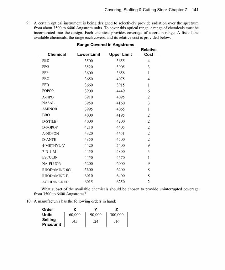
9. A certain optical instrument is being designed to selectively provide radiation over the spectrum

from about 3500 to 6400 Angstrom units. To cover this optical range, a range of chemicals must be

incorporated into the design. Each chemical provides coverage of a certain range. A list of the

available chemicals, the range each covers, and its relative cost is provided below.

Range Covered in Angstroms

Chemical

Lower Limit

Upper Limit

Relative Cost

PBD 3500 3655 4

PPO 3520 3905 3

PPF 3600 3658 1

PBO 3650 4075 4

PPD 3660 3915 1

POPOP 3900 4449 6

A-NPO 3910 4095 2

NASAL 3950 4160 3

AMINOB 3995 4065 1

BBO 4000 4195 2

D-STILB 4000 4200 2

D-POPOP 4210 4405 2

A-NOPON 4320 4451 2

D-ANTH 4350 4500 2

4-METHYL-V 4420 5400 9

7-D-4-M 4450 4800 3

ESCULIN 4450 4570 1

NA-FLUOR 5200 6000 9

RHODAMINE-6G 5600 6200 8

RHODAMINE-B 6010 6400 8

ACRIDINE-RED 6015 6250 2

What subset of the available chemicals should be chosen to provide uninterrupted coverage

from 3500 to 6400 Angstroms?

10. A manufacturer has the following orders in hand:

Order X Y Z

Units 60,000 90,000 300,000

Selling Price/unit

.45 .24 .16


Each order is for a single distinct type of product. The manufacturer has four different

production processes available for satisfying these orders. Each process produces a different

combination of the three products. Each process costs $0.50 per unit. The manufacturer must satisfy

the volumes specified in the above table. The manufacturer formulated the following LP:

Min .5 A + .5 B + .5 C + .5 D

s.t.

A >= 60000

2 B + C >= 90000

A + C + 3 D >= 300000

a) Which products are produced by process C?

b) Suppose the agreements with customers are such that, for each product, the manufacturer

is said to have filled the order if the manufacturer delivers an amount within + or − 10%

of the “nominal” volume in the above table. The customer pays for whatever is delivered.

Modify the formulation to incorporate this more flexible arrangement.

11. The formulation and solution of a certain staff-scheduling problem are shown below:

MIN M + T + W + R + F + S + N

T + W + R + F + S >= 14

W + R + F + S + N >= 9

M + R + F + S + N >= 8

M + T + F + S + N >= 6

M + T + W + S + N >= 17

M + T + W + R + N >= 15

M + T + W + R + F >= 18

END

Optimal solution found at step: 4

Objective value: 19.0000000

Variable Value Reduced Cost

M 5.000000 .0000000

T .0000000 .0000000

W 11.00000 .0000000

R .0000000 .0000000

F 2.000000 .0000000

S 1.000000 .0000000

N .0000000 .3333333

Row Slack or Surplus Dual Price

2 .0000000 -.3333333

3 5.000000 .0000000

4 .0000000 -.3333333

5 2.000000 .0000000

6 .0000000 -.3333333

7 1.000000 .0000000

8 .0000000 -.3333333


where, M, T, W, R, F, S, N is the number of people starting their five-day work week on Monday,

Tuesday, Wednesday, Thursday, Friday, Saturday, and Sunday respectively.

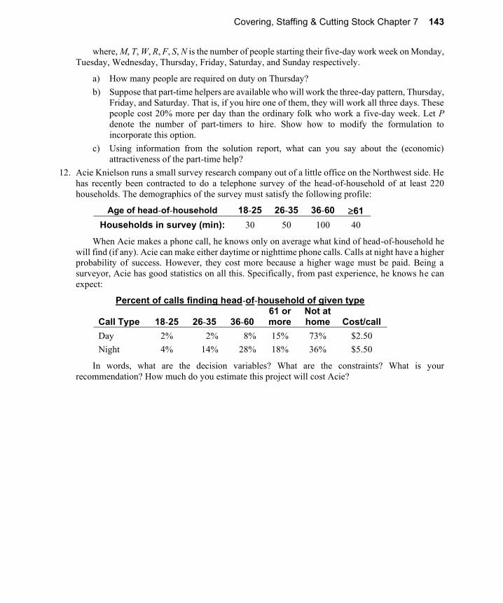
a) How many people are required on duty on Thursday?

b) Suppose that part-time helpers are available who will work the three-day pattern, Thursday,

Friday, and Saturday. That is, if you hire one of them, they will work all three days. These

people cost 20% more per day than the ordinary folk who work a five-day week. Let P

denote the number of part-timers to hire. Show how to modify the formulation to

incorporate this option.

c) Using information from the solution report, what can you say about the (economic)

attractiveness of the part-time help?

12. Acie Knielson runs a small survey research company out of a little office on the Northwest side. He

has recently been contracted to do a telephone survey of the head-of-household of at least 220

households. The demographics of the survey must satisfy the following profile:

Age of head-of-household 18-25 26-35 36-60 61

Households in survey (min): 30 50 100 40

When Acie makes a phone call, he knows only on average what kind of head-of-household he

will find (if any). Acie can make either daytime or nighttime phone calls. Calls at night have a higher

probability of success. However, they cost more because a higher wage must be paid. Being a

surveyor, Acie has good statistics on all this. Specifically, from past experience, he knows he can

expect:

Percent of calls finding head-of-household of given type Call Type

18-25

26-35

36-60

61 or more

Not at home

Cost/call

Day 2% 2% 8% 15% 73% $2.50

Night 4% 14% 28% 18% 36% $5.50

In words, what are the decision variables? What are the constraints? What is your

recommendation? How much do you estimate this project will cost Acie?


13. A political candidate wants to make a mass mailing of some literature to counteract some nasty

remarks his opponent has recently made. Five mailing lists have been identified that contain names

and addresses of voters our candidate might like to reach. Each list may be purchased for a price. A

partial list cannot be purchased. The numbers of names each list contains in each of four professions

are listed below.

Names on Each List (in 1000’s) by Profession Mailing

List

Law

Health Business

Executives Craft

Professionals Cost of

List

1 28 4 7 2 41,000

2 9 29 11 3 52,000

3 6 3 34 18 61,000

4 2 4 6 20 32,000

5 8 9 12 14 43,000

Desired

Coverage 20 18 22 20

Our candidate has estimated how many voters he wants to reach in each profession. This is

listed in the row “Desired Coverage”. Having a more limited budget than the opponent, our

candidate does not want to spend any more than he has to in order to “do the job”.

a) How many decision variables would you need to model this problem?

b) How many constraints would you need to model this problem?

c) Define the decision variables you would use and write the objective function.

d) Write a complete model formulation.

14. Your agency provides telephone consultation to the public from 7 a.m. to 8 p.m., five days a week.

The telephone load on your agency is heaviest in the months around April 15 of each year. You

would like to set up staffing procedures for handling this load during these busy months. Each

telephone consultant you hire starts work each day at either 7, 8, 9, 10, or 11 a.m., works for four

hours, is off for one hour, and then works for another four hours. A complication that has become

more noteworthy in recent years is that an increasing fraction of the calls handled by your agency

is from Spanish-speaking clients. Therefore, you must have some consultants who speak Spanish.

You are able to hire two kinds of consultants: English-speaking only, and bilingual (i.e., both

English- and Spanish-speaking). A bilingual consultant can handle English and Spanish calls

equally well. It should not be surprising that a bilingual consultant costs 1.1 times as much as an

English-only consultant. You have collected some data on the call load by hour of the day and

language type, measured in consultants required, for one of your more important offices. These data

are summarized below:

Hour of the day: 7 8 9 10 11 12 1 2 3 4 5 6 7

English load: 4 4 5 6 6 8 5 4 4 5 5 5 3

Spanish load: 5 5 4 3 2 3 4 3 2 1 3 4 4

For example, during the hour from 10 a.m. to 11a.m., you must have working at least three

Spanish-speaking consultants plus at least six more who can speak English.

How many consultants of each type would you start at each hour of the day?


15. The well-known mail order company R. R. Bean staffs its order-taking phone lines seven days per

week. Each staffer costs $100 per day and can work five consecutive days per week. An important

question is: Which five-day interval should each staffer work? One of the staffers is pursuing an

MBA degree part-time and, as part of her coursework, developed the following model specific to

R. R. Bean’s staffing requirements.

MIN=500 * M + 500 * T + 500 * W + 500 * R + 500 * F

+ 500 * S + 500 * N;

[R1] M + R + F + S + N >= 6 ;

[R2] M + T + F + S + N >= 7 ;

[R3] M + T + W + S + N >= 11;

[R4] M + T + W + R + N >= 9 ;

[R5] M + T + W + R + F >= 11;

[R6] T + W + R + F + S >= 9;

[R7] W + R + F + S + N >= 10;

END

Note that M denotes the number of staffers starting on Monday, T the number starting on

Tuesday, etc. R1, R2, etc., simply serve as row identifiers.

a) What is the required staffing level on Wednesday (not the number to hire starting on

Wednesday, which is a harder question)?

b) Suppose you can hire people on a 3-day-per-week part-time schedule to work the pattern

consisting of the three consecutive days, Wednesday, Thursday, Friday. Because of

training, turnover, and productivity considerations of part-timers, you figure the daily cost

of these part-timers will be $105 per day. Show how this additional option would be added

to the model above.

c) Do you think the part-time option above might be worth using?

d) When the above staffing requirements are met, there will nevertheless be some customer

calls that are lost, because of the chance all staffers may be busy when a prospective

customer calls. A fellow from marketing who is an expert on customer behavior and knows

a bit of queuing theory estimates having an additional staffer on duty on any given day

beyond the minimum specified in the model above is worth $75. More than one above the

minimum is of no additional value. For example, if the minimum number of staffers

required on a day is 8, but there are actually 10 on duty, then the better service will generate

$75 of additional revenue. A third fellow, who is working on an economics degree

part-time at Freeport Community College, argues that, because the $75 per day benefit is

less than the $100 per day cost of a staffer, the solution will be unaffected by the $75

consideration. Is this fellow’s argument correct?

e) To double check your answer to (b), you decide to generalize the formulation to incorporate

the $75 benefit of one-person overstaffing. Define any additional decision variables needed

and show (i) any modifications to the objective function and to existing constraints and (ii)

any additional constraints. You need only illustrate for one day of the week.


16. In a typical state lottery, a player submits an entry by choosing six numbers without replacement

(i.e., no duplicates) from the set of numbers {1, 2, 3, ..., 44}. After all entries have been submitted,

the state randomly chooses six numbers without replacement from the set {1, 2, 3,..., 44}. If all of

your six numbers match those of the state, then you win a big prize. If only five out of six of your

numbers match those of the state, then you win a medium size prize. If only four out of six of your

numbers match those of the state, then you win a small prize. If several winners chose the same

set of numbers, then the prize is split equally among them. You are thinking of submitting two

entries to the next state lottery. A mathematician friend suggests the two entries: {2, 7, 1, 8, 28,

18} and {3, 1, 4, 15, 9, 2}. Another friend suggests simply {1, 2, 3, 4, 5, 6} and {7, 8, 9, 10, 11,

12}. Which pair of entries has the higher probability of winning some prize?

17. For most cutting stock problems, the continous LP solution is close to the IP solution. In

particular, you may notice that many cutting stock problems possess the “integer round-up”

feature. For example, if the LP solution requires 11.6 sets, then that is a good indication that

there is an IP solution that requires exactly 12 sets. Does this round-up feature hold in general?

Consider for example a problem in which there is a single raw material of width 600 cm. There

are three finished good widths: 300 cm, 200 cm, and 120 cm, with requirements respectively of

3, 5, and 9 units.

7 covering, staffing & cutting stock models

Documents