TUMTECHNISCHE UNIVERSITÄT MÜNCHENINSTITUT FÜR INFORMATIK

TechnischerTechnische Universität MünchenInstitut für InformatikBericht

SYMBIOTIC TRAFFIC SIMULATIONFRAMEWORK

TUM-I1651

Abhinav Sunderrajan, Vaisagh Viswanathan,Wentong Cai, Alois Knoll

SYMBIOTIC TRAFFIC SIMULATIONFRAMEWORK

Abhinav Sunderrajan,1∗ Vaisagh Viswanathan,1 Wentong Cai2, Alois Knoll3

1TUM CREATE Ltd1 CREATE Way 138602, SINGAPORE

2School of Computer EngineeringNanyang Technological University Nanyang Avenue 639798, SINGAPORE

3Robotics and Embedded Systems Group Department of InformaticsTechnische Universitat Munchen Boltzmannstraße 3 D-85748 Garching bei Munchen, GERMANY∗To whom correspondence should be addressed; E-mail: abhinav.sunderrajan@tum-create.edu.sg

Real time data from several traffic participants such as smart-phone users and

vehicles equipped with GPS devices (taxi and bus fleets) is potentially available

in the form of a continuous data stream in several mega cities. This real time

data can be augmented with that from the traditional sensors for the imple-

mentation of several advanced traffic management and control strategies. In

this report we present and evaluate a data driven adaptive solution for traffic

flow optimization of a real world expressway by employing short-term predic-

tive simulations.

1 INTRODUCTION

A dynamic data driven adaptive simulation (DDDAS) incorporates real-time data from the

physical system to initialize or steer the simulation system. Symbiotic Simulation, introduced

in (1) is a special class of DDDAS involving a mutually beneficial relationship between the

1

physical system and simulation systems. The physical system provides continuous inputs to

steer the simulation which, in turn gives recommendations to the former.

In this report, we present a symbiotic traffic simulation framework which consists of a phys-

ical system and prediction & traffic-flow optimization system. The prediction & optimization

module receives continuous inputs from the physical system, i.e., the road network to initialize

predictive faster-than-real-time simulations. Based on the results of the predictive simulations,

a recommendation is sent back to control the road network for optimizing traffic flow. The

physical system is emulated using a high-fidelity agent based microscopic traffic simulation

incorporating acceleration and lane change models. The prediction & control system which

receives traffic state inputs from the physical system uses a macroscopic traffic flow model to

employ a simulation based optimization strategy. The recommendations of this predictive &

control system are given back to the physical system (microscopic simulation) and evaluated

for efficacy. Towards this end, the contributions of this report are as follows

• Develop a framework for symbiotic traffic simulation with the physical system providing

continuous inputs to the predictive & control system while getting back recommendations

to optimize traffic flow.

• Employ the predictive simulations for evaluating several control actions before sending

the best recommendation to the physical system. The control action chosen for this proof-

of-concept report is ramp-metering.

• Evaluate the efficacy of the recommendations given by the predictive & control system (in

the physical system) on employing ramp-metering by simulating a real world expressway.

2

2 RELATED WORK

The challenges of incorporating real-time data streams to steer executing simulations have been

discussed in (2). Dynamic data driven simulations have found applications in several domains.

An emergency detection and response system by (3) has been developed by processing call

data records in real-time for identifying anomalies and emergencies. Plans for further actions

when emergencies are detected are determined by agent based simulations. (4) have employed

multi-agent data driven simulations for reliable and efficient dispatching of electricity under

distributed generation for smart grids. Simulation based short-term forecasting using real-time

data streams has found applications in modeling and tracking wildfires by (5) and ocean state

observation and forecasting by (6).

The motivation for a city-scale symbiotic traffic-simulation can be found in (7). The pa-

per discusses a scenario where hundreds of white-box and gray-box agents provide real-time

measurements regarding their geo-location and speed (both white and gray-box agents) and

origin-destination (white-box agents only). Considering the burgeoning potential for the avail-

ability of traffic data from floating cars and other fixed sensors, it is likely that this real-time

data will be beneficial for various ITS based services such as dynamic ramp-metering which is

discussed in this report.

3 SYSTEM OVERVIEW

We employ an agent-based microscopic traffic simulation for a realistic representation of the

physical world. Microscopic simulations were employed owing to the enormous amount of

resources required to implement the recommendations of the predictive simulation on a real

world road network. The floating car data (FCD) provided by the microscopic simulation

was used to initialize the state of the predictive Cell Transmission Model (CTM) (8) based

3

PHYSICAL SYSTEM

Represented by an agent based microscopic simulation

PREDICTION & CONTROL SYSTEM

Current traffic state in number of vehicles, mean speed and standard deviation of speed of all cells.

Recommendations for optimizing traffic flow.

Turn ratios at off ramps and mean inter-arrival times at all source links

Optimization module

CTM basedpredictive

macroscopic simulation

Figure 1: Symbiotic traffic simulation system.

macroscopic simulation. Figure 1 illustrates the symbiotic relationship between the physical

and the prediction & control system.

The predictive component works hand-in-hand with the optimization module to give rec-

ommendations to the physical system to optimize traffic flow after evaluating several candidate

solutions. In this report, we optimize the traffic flow of a real world expressway (described

in Section 7.2) by employing ramp-metering as the control action. The near optimal ramp-

metering strategy is determined by the optimization module.

The primary reason for employing a macroscopic simulation for the predictive component,

is computational efficiency. A gradient-based optimization strategy involves assessing the fit-

ness of several candidate solutions in parallel. The fitness of a solution is given at the end of a

stochastic predictive traffic simulation over a predetermined time horizon. The above argument

motivates us to go in for a cell based macroscopic model despite the relative lack of accuracy

in comparison to the microscopic models. The execution time of a CTM based algorithm is

proportional to the number of cells simulated thus making it an ideal model for a prediction and

control system.

4

A microscopic traffic model involves simulating hundreds of thousands of agents and up-

dating their speeds and positions at every time-step. Further, modeling lane changes involves

acquiring locks (in the context of parallel programming) on multiple lanes making a large scale

microscopic simulation computationally expensive (See (9)). In the subsequent sections we

show that our calibrated first-order traffic simulation can model the evolution of traffic state

with minimal error (in comparison to the high fidelity microscopic models) provided it is well

calibrated and initialized with a reasonably good estimate of the current traffic state in the phys-

ical system.

4 PHYSICAL SYSTEM

The agent based traffic simulation representing the physical system is based on the SEMSim

platform (9, 10). SEMSim is a high fidelity agent-based microscopic simulation. It uses the

Intelligent Driver Model (IDM) (11) and MOBIL (12) as the acceleration and lane change mod-

els respectively. IDM is an accident free model which ensures that a vehicle attains the desired

velocity at free flow and maintains the safe bumper to bumper distance to the leading vehicle.

It also ensures that the acceleration is an increasing function of the speed and distance to the

leading vehicle and a decreasing function of its speed. MOBIL, the lane change model ensures

that the resultant accelerations and decelerations for a vehicle and its followers in the old and

new lanes does not exceed a safe threshold. A lane change is done only if a vehicle gains speed

without violating the safety and inconvenience (to the old and new followers) criteria.

The simulation takes as input a road network detailing the lanes constituting the roads to

be simulated. Road segments that don’t have a preceding road segment are considered sources

and those without a subsequent segment are sinks. The traffic thus flows from the sources to the

sinks. The route taken by each agent is determined based on turn ratios (ranging between 0.0

and 1.0) specified at each off-ramp. Parameters such as average vehicle length, the acceleration

5

and deceleration terms of IDM are modeled as distributions to take into account heterogeneous

driving behaviors and vehicle classes. Note that SEMSim and the term physical system shall be

used interchangeably over the rest of this report.

4.1 SEMSim Parameters

Simulationparameter Description Value

ST Simulation time 7200 sec

s0Minimum bumper-to-bumper distance

to the front vehicle. 2.0 m

T Time gap to preceding agent 1.4 sec

li Vehicle lengthNormal distribution withµ = 3.0 m and σ = 0.1 m

V0 Desired speed of agent 20 m/s

a Maximum acceleration term for IDMUniform distribution between

1.2 and 1.6 m/s2

b Maximum deceleration term for IDMUniform distribution between

1.8 and 2.2 m/s2

p0 Politeness factor for MOBIL 0.3∆ath Lane change threshold for MOBIL 0.3 m/s2

Table 1: The microscopic simulation parameters

SEMSim was initialized with the parameters listed in Table 1. Parameters such as a, b and

li are modeled as distributions to take into account heterogeneous driving behaviors and vehicle

classes.

5 MODELING OF PREDICTION SYSTEM

The predictive, faster-than-real-time macroscopic simulation is based on the stochastic variant

of the Cell Transmission Model (13) and METANET (14). The cell network, C is comprised of

n cells. At each time instant, t = k.Tctm, k = 0,1, ....K (where K is the time horizon) the state of

6

all cells are updated. The discrete event time step is denoted by Tctm.

The state of a cell ci ∈ C at each time step k is determined by sending Si(k) and receiving

potentials Ri(k). Si(k) and Ri(k) represent the number of vehicles cell ci can send and receive

at time-step k. The mean and standard deviation of speed for a cell ci are denoted by vi(k) and

vσi (k) respectively. The number of vehicles in a cell ci at time-step k is given by Ni(k). While

Nmaxi (k) represents the maximum number of vehicles that can be accommodated in cell ci given

an average speed of vi(k). Nmaxi (k) is given by

Nmaxi (k) =

li.λi

Tgap.vi(k)+Le f f(1)

where Le f f , the effective vehicle length represents the sum of mean vehicle length and minimum

gap. Tgap represents the safe time gap. The length of cell ci is denoted by li which is a variable

and subject to the constraint li ≤V i0×Tctm. V i

0 is the constant free-flow speed for the cell. This

constraint ensures that no vehicle can enter and exit a cell within one time-step. The number

of lanes in cell ci corresponding to the associated road-link is denoted by λi. The outflow in

number of vehicles at time-step k from cell ci is given by yi(k) and the density in number of

vehicles per unit distance per lane is denoted by ρi(k). The critical density ρcriti separating free

and congested traffic of a cell ci is given by

ρcriti =

1V i

0.Tgap +Le f f(2)

Other constants in this predictive simulation are the terms κ,δ and φ . The constants κ and

δ adapt the speed of the vehicles after an on-ramp expressway merge while last term φ adapts

the speed of cell where a lane drop occurs. V outmin denotes the minimum speed of cell a when it

is completely congested. V outmin thus models the fact that some vehicles exit a bottleneck with a

minimum speed. Finally, Am is a parameter of the fundamental diagram representing the speed

density relationship (See (14)).

7

Algorithm 1 CTM based macroscopic predictive simulation.1: while t < K do2: for each ci ∈ C do3: update sending and receiving potentials.4: for each ci ∈ C do5: update outflow.6: for each ci ∈ C do7: update number of vehicles.8: update density.9: for each ci ∈ C do

10: update average speed vi11: update the maximum number of vehicles Nmax

i

12: t = t + k.Tctm

C1

Source Cell

Sink Cell

Merging Cell

Diverging Cell

Ordinary Cell

Direction of flow of traffic along the main expressway

On Ramp Off Ramp

C2 C

3 C4

C5

C6

C7

C8

C9 C 10

C 11

Figure 2: An illustrative cell network.

8

The cells constituting the cell network C are classified into five different types as shown

in Figure 2. Note that this is an illustrative network and not the real world expressway (see

Section 7.2) simulated for the experiments. The Merging cells are associated with the parameter

merge priority µ ∈ [0.0,1.0] which controls the proportion of vehicles that moves to the next

cell in a given time-step. Correspondingly µonramp and µexp are the merge priorities of the on-

ramp and expressway cells respectively. The source and sink cells are not physically related

to any of the road links. The source and sink cells are effectively ghost cells since they have

zero length and zero lanes. The former injects agents into the simulation while the agents exit

the simulation through the latter. A Diverging cell is associated with the turn ratios τ ranging

between 0.0 and 1.0 representing the proportion of vehicles exiting the expressway through off

ramp and those continuing to traverse along the expressway. Cells C3 and C9 are considered

predecessors of cell C4. Similarly, cells C10 and C7 are considered successors of cell C6.

Algorithm 1 shows the progress of the simulation over the prediction time horizon K. The

equations governing the state of all cells at each time step are provided in the Appendix 10.

6 OPTIMIZATION MODULE

We implemented a particle swarm optimization (PSO) (15) approach (Algorithm 2) for the

optimization module to determine the best control strategy for the case study described later in

Section 7. The PSO algorithm seeks to identify the best control-action by minimizing the value

returned by the function f itness(~x) (~x represents a candidate solution) running the CTM based

predictive simulation over a time horizon K. Specifically, the fitness function returns the value J

(Equation 3) which represents the weighted average of total time spent (TTS) and total distance

traveled (TTD) over the time horizon K and over M cells (16).

9

Algorithm 2 Particle Swarm Optimization1: swarmSize, maxiter← swarm size and maximum iterations for PSO respectively.2: P←∅, the set of particles in the swarm.3: α ← proportion of velocity to be retained.4: β ← proportion of personal best to be retained.5: γ ← proportion of informant’s to be retained.6: δ ← proportion of global best to be retained.7: for swarmSize times do8: P← P

⋃new particle~x with initial velocity~v

9: ~Best←∅10: iter← 011: repeat12: for each~x ∈ P do13: if ~Best ==∅ or f itness(~x)< f itness( ~Best) then14: ~Best←~x15: Z← ∅16: for each~x ∈ P with velocity~v do17: ~x∗ previous fittest location of~x18: ~x+ previous fittest location of informants of~x19: ~x ! previous fittest location of any particle20: for each xi ∈~x do21: b← random number 0.0 to β inclusive22: c← random number 0.0 to γ inclusive23: d← random number 0.0 to δ inclusive24: vi← αvi +b(x∗i − xi)+ c(x+i − xi)+d(x!

i− xi)

25: for each~x ∈ P do26: ~x←~x+~v27: iter← iter+128: until iter < maxiter29: return ~Best

10

J = T.K

∑k=0

M

∑i=1

λi.li[αT T Sρi(k)−αT T D.ρi(k).vi(k)] (3)

The algorithm seeks to minimize the total number of vehicles while maximizing traffic flow

over K. Note that αT T S & αT T D ∈ (0.0,1.0). The PSO algorithm is a population-based method

where existing population members (or particles) are tweaked in response to new discoveries in

the search space. At each iteration, the fitness of every individual (Equation 3) is assessed using

the predictive simulation. Each particle is then tweaked based on the best global, informant’s

and personal solutions obtained thus far. The informants of a particle ~x refer to a small subset

of particles from the population which are chosen randomly each at iteration.

7 CASE STUDY

7.1 Ramp Metering

Ramp-metering is a traffic control mechanism implemented in several cities across the world

to reduce the congestion on expressways (17). Ramp meters are traffic signals placed at the

intersection of on-ramps and expressways. They regulate the flow of vehicles along the ramps

so as to minimize the turbulence caused due to merging vehicles disrupting the mainline flow.

Care must be taken to ensure that the queue of the vehicles waiting along the on-ramps does not

spill into the preceding urban street network.

Ramp-metering strategies are classified into two types: fixed-time and reactive (18). The

fixed time strategy is based on historical data pertaining to flow rates along the on-ramps and

the expressway at different times of the day. The main drawback of the fixed time strategy is

that their settings are based on historic rather than real time data. It does not take into account

the varying nature of traffic demand and the occurrence of events such as accidents and road

blocks which could cause massive congestions.

11

Reactive ramp-metering strategies aim to optimize the flow of traffic based on real-time

measurements. Reactive ramp-metering is classified into two types: Local Ramp-Metering and

Multivariable Regulator Strategies (18). The former makes use of measurements in the vicinity

of an on-ramp to regulate the flow on the ramp. The control strategy applied for an on-ramp is

independent of the measurements and controls applied in other on-ramps in the vicinity. The

latter makes use of the system wide measurements to simultaneously regulate traffic flow along

all on-ramps. A review on several implemented and proposed ramp-metering strategies can be

found in (17).

In this report we employ particle swarm optimization described in Section 6 to develop a

system wide ramp-metering strategy of a real world expressway by regulating the flow on all

on-ramps simultaneously. The system-wide ramp controller designed for this report determines

the maximum allowable queue-threshold qthr (Equation 4) for a ramp r ∈ Ron

ramps before turning

the phase of the signal to green from red, where Ronramps is the set of controllable on-ramps in

the system.

Nr(k)Nmax

r (k)≤ qth

r (4)

Where Nr(k) and Nmaxr (k) is the number and the maximum number of vehicles on the on-

ramp r at time step k. Nmaxr (k) at time-step k is determined from Equation 1. Concretely,

the task is to find the ideal value of qthr for all on-ramps so as to minimize Ntotal . Note that

qthr ∈ [0.0,1.0].

7.2 Simulated Physical Environment

For the experiments in this report, we simulate a 13 km stretch of P.I.E (Pan Island Expressway)

in central Singapore (Figure 3) with all on and off ramps. The on ramps and the first P.I.E link

12

Figure 3: Simulated section of P.I.E (Singapore) and location of all on/off ramps.

are sources, while all off ramps and the last link on P.I.E are sinks. Refer to the Table 3 for

the location of all on/off ramps (or static bottlenecks) starting from the beginning of the first

road-segment on P.I.E. The average distance between two bottlenecks is around 565 m along

this stretch of P.I.E. The turn ratios for all off-ramps is kept constant at 0.25. This implies that

25% of all vehicles exit at a given off ramp while the remaining 75% of the vehicles continue to

travel on the main expressway. The number of lanes in the simulated stretch of the expressway

varies between 3 and 6.

DISTANCE (m) RAMP TYPE583.98 On Ramp1973.35 Off Ramp2489.87 On Ramp3261.27 Off Ramp4071.9 On Ramp4834.84 Off Ramp5531.18 On Ramp5743.11 Off Ramp5965.29 On Ramp6207.74 Off Ramp

DISTANCE (m) RAMP TYPE7025.15 On Ramp7658.4 On Ramp

8040.83 Off Ramp8554.28 On Ramp8807.94 Off Ramp9591.84 On Ramp

10148.24 Off Ramp11286.2 On Ramp

11637.04 On Ramp12438.23 Off Ramp

Table 2: Location of all On/Off ramps along the expressway.

13

7.3 Traffic Scenario

Table 3: Mean inter-arrival times at all source links/cells

DISTANCE (m) RAMP TYPE εs (sec)0.0 First P.I.E link 1.0

583.98 On-Ramp 2.02489.87 On-Ramp 3.64071.9 On-Ramp 3.65531.18 On-Ramp 3.65965.29 On-Ramp 3.6

DISTANCE (m) RAMP TYPE εs (sec)7025.15 On-Ramp 2.07658.4 On-Ramp 2.0

8554.28 On-Ramp 3.69591.84 On-Ramp 3.611286.2 On-Ramp 3.6

11637.04 On-Ramp 3.6

The traffic state of the expressway at the end of a time horizon is determined by the inter-

arrival time εs for all source links and cells. The stretch of the expressway simulated consisting

of 11 on-ramps and along with the first expressway link has 12 source links/cells. Table 3 lists

the mean inter-arrival times for all source links/cells. Notice that the flow of vehicles into the

expressway along all on-ramps are significantly less (1000 vehicles/hour) except for the ones

at 583 m, 7025 m and 7658 m. The optimization module thus needs to find a ramp metering

strategy which balances the flow along all on-ramps so as to minimize the surge of vehicles

along the three ramps with relatively higher inflow of vehicles.

8 RESULTS

8.1 Calibration of Predictive Simulation

To ensure that the state predicted by the macroscopic simulation accurately represents the state

of the physical system, the model parameters have to be calibrated. We need to identify (and

tune) the parameters which will have significant impact in terms of bridging the difference in

the state of the physical system and that of the predictive simulation at the end of a given time

horizon.

14

Towards this end we simulated SEMSim representing the physical system over a time hori-

zon K = 2000 seconds. The mean inter-arrival times of all source links εs were kept constant

during the time period of the simulation. There are no vehicles in the simulation at time-step

k = 0. Nsemsimi (K) denotes the number of vehicles in each cell of the mainline expressway (cor-

responding to the cell-network associated with the predictive system) is computed at the end of

the microscopic agent-based simulation.

The initial state and the mean inter-arrival times of vehicles for all source cells εs are the

same as SEMSim for the predictive simulation. The turn ratios at the off-ramp (τo f framp) and

expressway (τexp) intersections are also the same as that of the physical system. The time-step

Tctm for the predictive simulation is kept constant at 4.0 seconds. To identify and then tune

the parameters which bridge the difference between the predictive simulation and the physical

system, we attempt to minimize the least square error given by Equation 5√√√√i=nexp

∑i=1

(Nsemsimi (K)−Nctm

i (K))2 (5)

Where Nctmi (K) denotes the number of vehicles in each cell of the mainline expressway com-

puted at the end of the predictive simulation time horizon K. The least square error thus repre-

sents the difference between the number of vehicles for all expressway cells (numbering nexp) at

K. We ran the predictive simulation 1500 times to the return least square error for each of these

runs to generate 1600 data points. The parameters of the CTM based predictive simulation were

varied based on the range column of the Table 4.

LSE = β0−β1.µonramp +β2.Tgap +β3.T 2

gap +β4.Tgap.µonramp (6)

The polynomial regression with an R2 Statistic (a measure of model fit indicating the per-

centage of variance explained by the model) of 0.817 is shown in Equation 6. This model clearly

shows that the two dominant terms are Tgap and µonramp. Based on the results of the calibration,

15

Table 4: The predictive simulation parameters

Simulationparameter Description Range Calibrated

Value

µrampMerge priority for on ramp

merging cells [0,1,0.7] 0.45

µexpMerge priority for express way

merging cells. [0.8,0.1] 0.9

Tgap Safe time gap for vehicles (s) [1.2,1.5] 1.25V out

min Minimum speed in a cell (m/s) [2.0,6.0] 2.5 m/sδ On ramp merge term [0.02,0.6] 0.27

Am Model term of fundamental diagram [1.0,4.0] 2.34φ Lane drop term [1.8,3.6] 2.7κ On ramp merge term [0.1,2.0] 0.45

the CTM based predictive simulation was initialized with the parameters shown in Table 4. The

values of Am,φ ,κ and δ are chosen based on the calibration experiments by (14). Note that

V outmin is set to 0.0 for the on-ramps since the vehicles come to a complete standstill when the

signal is red.

8.2 Efficacy of Ramp Metering

In this section, we quantify the efficacy of using ramp-metering in the physical system (SEM-

Sim) based on the recommendations given by the predictive & control system. As discussed in

Section 7.1, we need to find the optimal value of qthr ∈ [0.0,0.8] for each of the 11 on-ramps for

the environment simulated. Note that the maximum value of the queue-threshold qthmax is set to

0.8. The controller sets the phase to green when qthr exceeds qth

max serving as the first constraint.

The other constraints are

1. The minimum phase time for both the red and green phases are 12 seconds.

2. The signal at an on-ramp can be continuously red only for a maximum of 120 seconds.

After a 120 second red phase, there is a mandatory green phase for 24 seconds.

16

The first of the above constraint ensures that the phase changes do not change rapidly. This

gives adequate reaction times for drivers to slow down and accelerate at an intersection. The

second constraint ensures that none of the vehicles wait at an on-ramp for an inordinately long

time thus preventing the starvation of an on-ramp r even if the qthr is not exceeded.

The fitness function f itness(~x) from Algorithm 2 has been modified to compute Jmean, the

mean of 5 different runs of CTM for a ramp-metering configuration ~x to account for model

stochasticity. Note that the term run of the predictive simulation refers to the execution of the

simulation over the time horizon K. The initial population size was set to 15 and the maximum

number of iterations was restricted to 25 (based on Figure 4). The parameters α,β ,γ and δ were

set to 0.9, 2.0, 2.0 and 2.0 respectively. The parameters in αT T S and αT T D used to compute the

fitness (Equation 3) J are set to 0.95 and 0.05 respectively.

100000

105000

110000

115000

120000

125000

130000

135000

1 2 3 4 5 6 7 8 9 10 11 12 13 14 15 16 17 18 19 20 21 22 23

Me

an f

itn

ess

iteration

Trial 1

Trial 2

Figure 4: Jmean vs iteration.

Figure 4 plots Jmean as a function of iteration count for two different trials of the PSO al-

gorithm running the CTM based predictive simulation. It can be observed that the algorithm

converges to a large extent in less than 25 iterations. The best ramp-meter configuration (deter-

mined using the predictive simulation) is now given as a recommendation to SEMSim which

returns the corresponding J over the same time horizon of 1800 seconds. Note that the con-

17

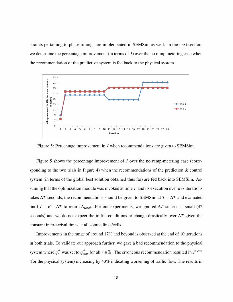
straints pertaining to phase timings are implemented in SEMSim as well. In the next section,

we determine the percentage improvement (in terms of J) over the no ramp metering case when

the recommendation of the predictive system is fed back to the physical system.

5

7

9

11

13

15

17

19

21

23

1 2 3 4 5 6 7 8 9 10 11 12 13 14 15 16 17 18 19 20 21 22 23

% im

pro

vem

en

t in

SEM

Sim

ove

r n

o r

amp

m

ete

rin

g

Iteration

Trial 1

Trial 2

Figure 5: Percentage improvement in J when recommendations are given to SEMSim.

Figure 5 shows the percentage improvement of J over the no ramp-metering case (corre-

sponding to the two trials in Figure 4) when the recommendations of the prediction & control

system (in terms of the global best solution obtained thus far) are fed back into SEMSim. As-

suming that the optimization module was invoked at time T and its execution over iter iterations

takes ∆T seconds, the recommendations should be given to SEMSim at T +∆T and evaluated

until T +K−∆T to return Ntotal . For our experiments, we ignored ∆T since it is small (42

seconds) and we do not expect the traffic conditions to change drastically over ∆T given the

constant inter-arrival times at all source links/cells.

Improvements in the range of around 17% and beyond is observed at the end of 10 iterations

in both trials. To validate our approach further, we gave a bad recommendation to the physical

system where qthr was set to qth

max for all r ∈R. The erroneous recommendation resulted in Jmean

(for the physical system) increasing by 43% indicating worsening of traffic flow. The results in

18

this section illustrates the potential of symbiotic traffic simulation as an effective tool for traffic

flow optimization through dynamic ramp-metering as a case study.

8.3 Note On The Computational Efficiency of Predictive Simulation

A data driven adaptive simulation and prediction framework for traffic systems should work

under reasonable time constraints for predicting short term evolution of state and giving back

recommendations to optimize traffic flow. The simulations employed by the predictive system

should thus be reasonably fast. The computational time for the CTM based simulation (used

for determining J) over a time horizon of 1800 seconds is around 75 milliseconds. The CTM

simulation was coded in Java SE 7 and measured in a 2.5 GHz Intel i5 system running on

Windows 7. The entire run of the PSO algorithm over 25 iterations took around 45 seconds

to complete, thus satisfying the soft real time constraints for a symbiotic traffic simulation.

The prediction & control system can give a recommendation much earlier (at the end of 40

iterations) to the physical system before searching for and further fine tuning the ramp control

strategy in the background.

9 CONCLUSIONS & FUTURE WORK

In this work we have established that data driven predictive simulations can be beneficial to-

wards optimizing traffic flow. The prediction and optimization system should receive fairly

accurate and continuous information on the current traffic state. This information is used for

initialization, calibration and steering of the predictive simulations. Accurate current state esti-

mation in turn increases the accuracy of the short term predictions (of evolution of traffic flow)

thereby increasing the efficacy of the suggested control measures. Data from traditional fixed

sensors can be augmented with FCD from smart phones and vehicle fleets such as taxis and

public buses for enhanced traffic state reconstruction. The simulation model and optimization

19

strategy used in the prediction & control system can be varied depending upon accuracy, effi-

cacy and computational time constraints.

Symbiotic traffic simulations also offer exciting opportunities to implement and optimize

several techniques for traffic flow optimization (other than ramp-metering discussed in this re-

port) such as adaptive speed limits and dynamic routing. Mobile applications and in car naviga-

tion systems provide a great means to disperse information to the traffic participants while the

control system receives user anonymized data about vehicle speed, location and even origin-

destination flows. This form of a symbiotic simulation based traffic prediction and optimization

framework directed towards dispersing and receiving updates from individual drivers will be

the focus of our future research.

10 APPENDIX. EQUATIONS FOR UPDATING CELL STATE

Updating Sending and Receiving Potentials for all ci ∈ C

term1 =Ni(k).vi(k).Tctm

li(7a)

term2 =Ni(k).V out

min .Tctm

li(7b)

Si(k+1) = min(max(term1, term2), Ni(k)) (7c)

Ri(k+1) = Nmaxi (k)−Ni(k) (7d)

Updating the outflow for all ci ∈ C The outflow of an Ordinary cell is given by,

yi(k+1) = min(Si(k+1), Ri+1(k+1)) (8)

The outflow of a Diverging cell is given by,

yo f framp(k+1) = min(τo f f

ramp.Si(k+1), Rrampi+1 (k+1)) (9a)

yexp(k+1) = min(τexp.Si(k+1), Rexpi+1(k+1)) (9b)

yi(k+1) = yo f framp(k+1)+ yexp(k+1) (9c)

20

where Rrampi+1 (k) and Rexp

i+1(k) represent the receive potential of the succeeding Ordinary cells on

the off-ramp and expressway respectively. While τexp and τo f framp represents the turn ratios for

the expressway and the off-ramp respectively.

The outflow of a Merging cell is given by,

term1 =µ.Ri+1(k+1)

µ +µother (10a)

yi(k+1) = min(term1, Si(k+1)) (10b)

Where µother and Sotheri (k+1) represents the merge-priority and the sending potential of the

other associated merging cell.

The outflow of a Source cell is given by,

yi(k+1) = min(randomPois(ε), Ri+1(k+1)) (11)

where randomPois(ε) represents the random Poisson number with a mean corresponding

to the average inter-arrival time (ε) for the source link. Note that Sink cell does not have any

outflow. Note that the outflow of a ramp cell is set to 0 when the signal phase is red.

Update number of vehicles in all cells

Ni(k+1) = Ni(k)− yi(k+1)+j=p

∑j=1

y j(k+1) (12)

Wherej=n∑j=0

y j(k) represents the total inflow from all of the p predecessors to this cell i where p

is either 1 or 2.

Update density and anticipated density for all ci ∈ C

ρi(k+1) =Ni(k+1)

li.λi(13a)

ρantici (k+1) = α.ρi(k)+(1−α).

j=s

∑j=1

ρ j(k+1) (13b)

21

Where ρantici (k + 1) is the anticipated density in the successor cell(s). It represents the

weighted average of the density in the current cell and those of its s successor cells. The co-

efficient α ∈ [0,1], we chose α to be 0.15 thus giving more importance to the density in the

successor cell(s) while not completely ignoring the current cell density.

Update Average speed and Nmaxi for all ci ∈ C

vtempi (k+1) =

j=p∑j=1

[v j(k).y j(k)]+ vi(k)(Ni(k)− yi(k)), if Ni(k+1) 6= 0

V0, otherwise(14)

vtempi (k+1) = max(vtemp

i (k+1), V outmin) (15a)

vi(k+1) = βi.vtempi (k+1)+(1−βi).V i

0.exp[−1Am

(ρantic

i (k+1)ρcrit

i

)Am]+η

sdi (15b)

where, βi =

0.8, if ρantici+1 (k+1)

ρantici (k+1)

or ρantici (k+1)

ρantici+1 (k+1)

≥ 1.8

0.2, otherwise(15c)

The lane drop term for the merging cell when vehicles merge at the expressway at the end

of an on-ramp.

vi(k+1) = vi(k+1)−φ .Tgap.ρi(k+1).vi(k+1)2

li.λi.ρcriti

(16)

The speed adaptation at the ordinary cell following the merge cells of the expressway and

the corresponding on-ramp. See cell C4 for reference in Figure 2.

vi(k+1) = vi(k+1)−δ .Tgap.yon

ramp(k+1).vi(k+1)λi.li(ρi(k+1)+κ)

(17)

Where yonramp(k+1) represents the outflow of an on-ramp cell.

Equation 15a ensures that the minimum speed of the cell does not fall below V outmin , i.e. the

minimum speed with which downstream vehicles exit congested zones. Equation 15b gives

greater weight to the anticipated density term (controlled by the parameter βi) if the absolute

22

difference in the density of the current and the successor cells is large. ηsdi is the random

Gaussian noise term with mean 0 and standard deviation vsdi . As noted before vsd

i is an input

from the physical system.

ACKNOWLEDGMENTS

This work was financially supported by the Singapore National Research Foundation under its

Campus for Research Excellence And Technological Enterprise (CREATE) programme.

References and Notes

1. R. Fujimoto, D. Lunceford, E. Page, Grand challenges for modeling and simulation, Tech.

Rep. No. 350, Dagstuhl report, Schloss Dagstuhl (2002). Seminar No 02351.

2. F. Darema, Computational Science-ICCS 2004 (Springer, 2004), pp. 662–669.

3. T. Schoenharl, G. Madey, G. Szabo, A.-L. Barabasi, Proceedings of the 3rd International

ISCRAM Conference (2006), vol. 1.

4. N. Celik, A. E. Thanos, J. P. Saenz, Procedia Computer Science 18, 1899 (2013).

5. C. C. Douglas, et al., Simulation Conference, 2006. WSC 06. Proceedings of the Winter

(IEEE, 2006), pp. 2117–2124.

6. N. Patrikalakis, et al., Dynamic Data-Driven Application Systems. Kluwer Academic Pub-

lishers, Amsterdam (2004).

7. H. Aydt, M. Lees, A. Knoll, Proceedings of the 2012 Winter Simulation Conference,

C. Laroque, J. Himmelspach, R. Pasupathy, O. Rose, A. M. Uhrmacher, eds. (Piscataway,

New Jersey: Institute of Electrical and Electronics Engineers, Inc., 2012), pp. 1–12.

23

8. C. F. Daganzo, Transportation Research Part B: Methodological 28, 269 (1994).

9. H. Aydt, Y. Xu, M. Lees, A. Knoll, AsiaSim 2013 (Springer, 2013), pp. 1–12.

10. D. Zehe, A. Knoll, W. Cai, H. Aydt, Simulation Modelling Practice and Theory 58, pages

157 (2015).

11. M. Treiber, A. Kesting, Intelligent Transportation Systems Magazine, IEEE 2, 6 (2010).

12. A. Kesting, M. Treiber, D. Helbing, Transportation Research Record: Journal of the Trans-

portation Research Board (2015).

13. R. Boel, L. Mihaylova, Transportation Research Part B: Methodological 40, 319 (2006).

14. A. Kotsialos, M. Papageorgiou, C. Diakaki, Y. Pavlis, F. Middelham, Intelligent Trans-

portation Systems, IEEE Transactions on 3, 282 (2002).

15. T. Weise, Self-Published, (2009).

16. M. Hadiuzzaman, T. Z. Qiu, Canadian Journal of Civil Engineering 40, 46 (2013).

17. K. Bogenberger, A. D. May, California Partners for Advanced Transit and Highways

(PATH) (1999).

18. M. Papageorgiou, C. Diakaki, V. Dinopoulou, A. Kotsialos, Y. Wang, Proceedings of the

IEEE 91, 2043 (2003).

24