5g mobile network architecture€¦ · furthermore, a new case study on elasticity is presented...
TRANSCRIPT

H2020-ICT-2016-2
5G-MoNArch
Project No. 761445
5G Mobile Network Architecture for diverse services, use cases, and applications in 5G and beyond
Deliverable D4.2
Final design and evaluation of resource elasticity framework
Contractual Date of Delivery 2019-03-31
Actual Date of Delivery 2019-04-10
Work Package WP4–Resource Elasticity
Editor(s) David GUTIERREZ ESTEVEZ (SRUK)
Reviewers Andrew BENNETT (SRUK), Carlos J. BERNARDOS (UC3M)
Dissemination Level Public
Type Report
Version 1.0
Total number of pages 156
Abstract: The roadmap towards the sustainable implantation of 5G networks necessarily passes
through its economic feasibility. Leveraging on the recent advantages in network orchestration and
Network Function Virtualisation (NFV), we have proposed the concept of resource elasticity for 5G
networks. By applying elasticity to the network lifecycle management, the network can flexibly adapt
to the changing demands (in both temporal and spatial domains), minimising both over-provisioning
and performance degradation and thus providing a better resource utilisation while fulfilling the
stringent KPIs that 5G services will require. This characteristic is even more important in a multi-
slice, multi-tenant network, where resource assignments shall be made on a per-slice basis. In the
previous 5G-MoNArch deliverable D4.1 we analysed elasticity from different perspectives: at VNF,
intra-, and inter-slice levels. In this final work package 4 deliverable, we further extend this analysis,
describing more in detail novel algorithms and solutions and identifying machine learning and
artificial intelligence as two key components for building network elasticity. Then, another main
contribution of this document is the elastic network architecture (that builds on and extends the ETSI
NFV and ENI ones) and the specific elastic resource orchestration use case. Finally, we discuss how
elasticity can be brought into practice by describing the elastic aspects of the 5G-MoNArch touristic
city testbed and the demonstrator that was specifically developed for showcasing elasticity.
Keywords: Resource Elasticity, 5G Architecture, Artificial Intelligence, Slice Lifecycle
Management, Resource Management, Elastic Network Functions.

5G-MoNArch (761445) D4.2 Final design and evaluation of resource elasticity framework
Version 1.0 Page 2 of 153
Executive Summary
This document is the final deliverable of work package 4 within the 5G-PPP 5G-MoNArch project
dedicated to the study of resource elasticity, one of the two key functional innovations introduced by
the project. In the first public deliverable of this work package [5GM-D41], we presented the
intermediate results focused around the following three dimensions of elasticity:
• Definition of an elastic architecture and workflow: The three main dimensions of resource
elasticity for 5G networks were identified (i.e., elasticity at Virtualised Network Function
(VNF) level, elasticity at intra-slice level, elasticity at infrastructure level). In addition, we
developed the foundations of an elastic functional architecture applied to 5G systems.
• Economic implications of resource elasticity: Business requirements were introduced by
analysing the economic implications of the concept of elasticity via system dimensioning as
well as adding economic views on the different technologies relevant to elasticity.
• Mechanisms for resource elasticity provisioning: An initial version of different specific
mechanisms and algorithms was proposed along its three identified dimensions, namely
computational elasticity, orchestration-driven elasticity, and slice-aware elasticity.
In this final deliverable, the above described work has been extended and brought to its completion.
Specifically, the following content has been added based on successfully accomplished research tasks:
• Architecture specification: We provide the full description of the elastic architecture,
complementing the overall architecture defined by 5G-MoNArch [5GM-D22] with the
specification of all relevant interfaces and high-level procedures for the elastic operation of the
network. Message Sequence Charts (MSCs) are introduced for elastic network operations along
the three dimensions of elasticity. In addition, each of these dimensions is mapped to the overall
architecture in terms of its relevant components. Furthermore, by introducing Artificial
Intelligence (AI) and analytics as a built-in feature to the network architecture, we effectively
propose an elastic and intelligent architecture. More specifically, we provide an extension of
the ETSI Experiential Network Intelligence (ENI) architecture, a piece of work currently
ongoing within this industry specification group. The rationale behind this choice is two-fold.
Firstly, the ETSI ENI architecture is, in turn, relying on the ETSI NFV architecture. As 5G-
MoNArch is fully considering ETSI NFV as baseline for the management and orchestration
architecture, the alignment of this architecture with the project one will be seamless. Secondly,
most of the solutions and algorithms devised in the work package 4 are actually relying on AI,
making them very suitable for this kind of approach.
• Mechanisms for resource elasticity: We further provide a full conceptual description of all
mechanisms and algorithms that were initially described in [5GM-D41]. In addition, a
comprehensive set of evaluation results for every mechanism is provided along with a novel
analysis on its impact on the relevant KPIs for elasticity defined in [5GM-D41].
• Cost-efficiency analysis: We provide a full description of the network cost-efficiency
enhancements brought by resource elasticity, with a highly comprehensive techno-economic
analysis that considers equipment aspects and their contributions to the overall network cost.
Furthermore, a new case study on elasticity is presented addressing the commercial feasibility
of temporary hotspots in MNO-driven deployments and emerging deployment models.
• Implementation aspects: The elasticity innovations being implemented in the 5G-MoNArch
Touristic City Testbed are described as some of the techniques and solutions described in this
document will be showcased in that framework, providing a view on how elasticity can improve
the network operation with a real-world service. Moreover, we have also developed an
experimental lab demonstration based on Open Air Interface (OAI) on elasticity at VNF level,
which is also described in this document. These practical insights further corroborate the
advantages of resource elasticity.
In terms of dissemination, this research work has resulted in numerous publications and standards
contributions, as well as several events organised for the broader research community. The interested
reader is referred to the project website for further information [5GM-w].

5G-MoNArch (761445) D4.2 Final design and evaluation of resource elasticity framework
Version 1.0 Page 3 of 153
List of Authors
Partner Name E-mail
NOK-DE Irina Balan [email protected]
UC3M Marco Gramaglia
Pablo Serrano
Cristina Marquez
Adolfo Santiago
DT Paul Arnold
Michael Einhaus
Igor Kim
Mohamad Buchr Charaf
SRUK David Gutierrez Estevez
Joan S. Pujol Roig
ATOS Jose Escobar
Jose Enrique González
CEA Antonio De Domenico
Nicola di Pietro
CERTH Asterios Mpatziakas
Stavros Papadopoulos
Anastasis Drosou
Eleni Ketzaki
MBCS Dimitris Tsolkas
Odysseas Sekkas
RW Julie Bradford
Abhaya Sumanasena
NOMOR Sina Khatibi [email protected]
Revision History
Revision Date Issued by Description
1.0 10.04.2019 5G-MoNArch WP4 Final submitted version 1.0
5G-MoNArch (761445) D4.2 Final design and evaluation of resource elasticity framework
Version 1.0 Page 4 of 153
Table of Contents
1 Introduction ................................................................................................ 13
1.1 Resource elasticity: a recap ...................................................................................... 13 1.2 The role of artificial intelligence and machine learning ........................................ 14 1.3 Document structure and contributions .................................................................... 14
2 The cost-efficiency potential of resource elasticity .................................. 17
2.1 Mapping elasticity to equipment and their contribution to overall network cost ... 17 2.2 Using elasticity to make temporary demand hotspots commercially viable ........... 20
2.2.1 Hotspot cost reductions from elasticity in an MNO driven deployment ....................... 22 2.2.2 Elasticity making emerging deployment models for hotspots more attractive .............. 26
3 Intelligent elastic architecture ................................................................... 28
3.1 An architectural framework for intelligent and elastic resource management and
orchestration ........................................................................................................................ 28 3.1.1 The role of AI in the architecture .................................................................................. 29 3.1.2 Actors and roles ............................................................................................................. 29
3.2 Architecture overview ............................................................................................... 29 3.3 Interfaces and message sequence charts enabling elasticity .................................. 31
3.3.1 Slice-aware elasticity ..................................................................................................... 31 3.3.2 Orchestration-driven elasticity ...................................................................................... 32 3.3.3 Computational elasticity ................................................................................................ 34
3.4 The ETSI ENI engine ............................................................................................... 36 3.4.1 ETSI ENI use case: elastic resource management and orchestration ............................ 37 3.4.2 Initial context configuration .......................................................................................... 37 3.4.3 Triggering conditions .................................................................................................... 38 3.4.4 Operational flow of actions ........................................................................................... 38 3.4.5 Post-conditions .............................................................................................................. 38
3.5 Overview of mechanisms for provisioning elasticity and placement in the
architecture .......................................................................................................................... 38 3.5.1 AI-based mechanisms .................................................................................................... 38 3.5.2 Elasticity in resource management and network function design ................................. 39
4 Intelligent elastic network lifecycle management .................................... 40
4.1 A taxonomy for learning algorithms in 5G networks ............................................. 40 4.2 Slice admission control mechanism ......................................................................... 42
4.2.1 Slice analytics for elastic network slice setup ............................................................... 42 4.2.1.1 Methodology .......................................................................................................... 43 4.2.1.2 Main results ........................................................................................................... 45
4.2.2 A resource market-based admission control algorithm ................................................. 46 4.2.2.1 Machine learning and neural networks framework .............................................. 46 4.2.2.2 Algorithm description ............................................................................................ 48 4.2.2.3 Performance evaluation ........................................................................................ 48
4.3 Intelligent VNF scaling and re-location .................................................................. 50 4.3.1 AI-assisted scaling and orchestration of NFs ................................................................ 51
4.3.1.1 System model ......................................................................................................... 51 4.3.1.2 Problem formulation ............................................................................................. 52 4.3.1.3 Cost ........................................................................................................................ 54 4.3.1.4 Actor-critic ............................................................................................................ 55 4.3.1.5 Numerical results................................................................................................... 56 4.3.1.6 Mapping to KPIs ................................................................................................... 58
4.3.2 Dynamic VNF deployment............................................................................................ 59 4.3.2.1 Problem statement ................................................................................................. 60

5G-MoNArch (761445) D4.2 Final design and evaluation of resource elasticity framework
Version 1.0 Page 5 of 153
4.3.2.2 Problem reformulation .......................................................................................... 62 4.3.2.3 Simulation results .................................................................................................. 63
4.4 Multi-objective resource orchestration .................................................................... 67 4.4.1 Resource allocation approach based on MOEA/D ........................................................ 68
4.4.1.1 Simulation data and scenarios description ........................................................... 70 4.4.2 Simulation results .......................................................................................................... 71
4.4.2.1 First scenario ........................................................................................................ 71 4.4.2.2 Second scenario ..................................................................................................... 73
4.4.3 KPI takeaways ............................................................................................................... 73 4.5 Slice-aware elastic resource management ............................................................... 74
4.5.1 AI-based slice-aware resource management ................................................................. 74 4.5.2 Slice-aware elastic resource management model .......................................................... 75 4.5.3 Computational resource provisioning ............................................................................ 78 4.5.4 Numerical results ........................................................................................................... 79
5 Elastic resource management .................................................................... 82
5.1 Data driven multi-slicing efficiency ......................................................................... 82 5.1.1 Networks scenario and metrics ...................................................................................... 83
5.1.1.1 Networks slicing scenario ...................................................................................... 83 5.1.1.2 Slice specification .................................................................................................. 84 5.1.1.3 Resource allocation to slices ................................................................................. 84 5.1.1.4 Multiplexing efficiency .......................................................................................... 85 5.1.1.5 Case studies ........................................................................................................... 85
5.1.2 Data driven evaluation ................................................................................................... 86 5.1.2.1 Slicing efficiency in worst case settings ................................................................ 86 5.1.2.2 Moderating slice specifications ............................................................................. 87 5.1.2.3 Orchestrating resources dynamically .................................................................... 87
5.1.3 Takeaways and KPI analysis ......................................................................................... 88 5.2 Slice-aware automatic RAN configuration.............................................................. 89
5.2.1 Detailed description of the solution ............................................................................... 89 5.2.2 Evaluation scenario and KPIs ........................................................................................ 91 5.2.3 Simulator enhancement description .............................................................................. 92 5.2.4 Simulation results and discussion .................................................................................. 93 5.2.5 Conclusions and link with KPIs .................................................................................. 101
5.3 Game theory approach to resource assignment .................................................... 101 5.3.1 Network slicing model ................................................................................................ 101
5.3.1.1 Resource allocation model .................................................................................. 101 5.3.1.2 Slice utility ........................................................................................................... 102 5.3.1.3 Network slicing framework .................................................................................. 103
5.3.2 Admission control for sliced networks ........................................................................ 103 5.3.2.1 Nash equilibrium existence .................................................................................. 104 5.3.2.2 Worst-case admission control (WAC) ................................................................. 104 5.3.2.3 Load-driven admission control (LAC) ................................................................. 105
5.3.3 Performance evaluation ............................................................................................... 106 5.3.3.1 Network utility ..................................................................................................... 106 5.3.3.2 Blocking probability ............................................................................................ 107
5.4 Slice-aware computational resource allocation .................................................... 107 5.4.1 Background ................................................................................................................. 107 5.4.2 Efficient resource utilisation........................................................................................ 108
5.4.2.1 Problem formulation ........................................................................................... 108 5.4.2.2 Proposed approach ............................................................................................. 109 5.4.2.3 Resource allocation algorithm ............................................................................ 110
5.4.3 Performance degradation model .................................................................................. 112 5.5 Profiling of computational complexity of RAN ..................................................... 114
5.5.1.1 Profiling over the air PHY layer ......................................................................... 115

5G-MoNArch (761445) D4.2 Final design and evaluation of resource elasticity framework
Version 1.0 Page 6 of 153
5.5.1.2 Profiling at MAC/RLC/PDCP layers .................................................................. 115
6 Elastic network functions ........................................................................ 118
6.1 Elastic RAN scheduling .......................................................................................... 118 6.1.1 Optimal solution .......................................................................................................... 120 6.1.2 Approximate solution: CARES algorithm ................................................................... 120
6.1.2.1 Algorithm description .......................................................................................... 120 6.1.3 Performance evaluation ............................................................................................... 121
6.1.3.1 Utility performance ............................................................................................. 122 6.1.3.2 Throughput distribution....................................................................................... 122 6.1.3.3 Large scale network ............................................................................................ 123 6.1.3.4 Savings in computational capacity ...................................................................... 123 6.1.3.5 Takeaways ........................................................................................................... 124
6.2 Elastic rank control for higher order MIMO ........................................................ 125
7 Practical aspects of resource elasticity ................................................... 132
7.1 Elastic aspects of the Turin testbed ........................................................................ 132 7.2 Computational elasticity demonstrator .................................................................. 133
7.2.1 Relation to 5G-MoNArch architecture ........................................................................ 133 7.2.2 Demonstrator setup ...................................................................................................... 134 7.2.3 Experiment with fixed SINR level .............................................................................. 136 7.2.4 Experiment with SINR process based on live network measurements ....................... 137
7.3 Monitoring tools for elastic operation ................................................................... 141 7.3.1 Challenges to monitoring containers ........................................................................... 144 7.3.2 E2E latency based on slices: difficulties measuring latency ....................................... 144 7.3.3 Monitoring privative/limited access VMs (unable to include exporters) .................... 145
8 Summary and conclusions ....................................................................... 146
References ........................................................................................................ 148

5G-MoNArch (761445) D4.2 Final design and evaluation of resource elasticity framework
Version 1.0 Page 7 of 153
List of Figures
Figure 2-1: Comparison between the equipment elements ................................................................... 17 Figure 2-2: Illustration of where the three dimensions of elasticity impact .......................................... 18 Figure 2-3: Hamburg city centre and sea port study area ...................................................................... 19 Figure 2-4: Assumed starting infrastructure in the study area ............................................................... 19 Figure 2-5: Indicative contribution of cost elements in the network cost ............................................. 20 Figure 2-6: Hamburg study area with demand hotspot from Steinwerder cruise ship terminal ............ 21 Figure 2-7: Elastic deployment model for serving temporary demand hotspots ................................... 21 Figure 2-8: Demand scenarios considered at the cruise ship terminal .................................................. 22 Figure 2-9: Calculated capacity per small cell over time ...................................................................... 23 Figure 2-10: Number of small cells required to serve the cruise ship terminal ..................................... 24 Figure 2-11: Number of cores used by macrocell/small cell networks ................................................. 25 Figure 2-12: 2020-2030 total cost of ownership for the small cell network ......................................... 25 Figure 2-13: Assumed spectrum availability between the deployment scenarios considered ............... 26 Figure 2-14: Comparison of the 2020-2030 total cost of ownership of the small cell .......................... 27 Figure 3-1: 5G-MoNArch overall functional architecture (top) ............................................................ 30 Figure 3-2: High level interactions across elastic modules ................................................................... 31 Figure 3-3: Information flow in case of service requirements update ................................................... 32 Figure 3-4: Information flow in case of performance degradation ....................................................... 32 Figure 3-5: Information flow after update of service requirements ...................................................... 33 Figure 3-6: Information flow in case of performance degradation ....................................................... 33 Figure 3-7: Message sequence chart for computational elastic operations ........................................... 35 Figure 3-8: Alternative Message sequence chart for computational elastic operations ........................ 35 Figure 3-9: Joint ETSI – 3GPP management and orchestration architecture ........................................ 37 Figure 3-10: Network slice instance lifecycle [TR28.801] ................................................................... 39 Figure 4-1: Innovations on elastic network lifecycle management ....................................................... 40 Figure 4-2: Learning taxonomy axes for slice lifecycle management ................................................... 41 Figure 4-3: Mapping of network slices to network function ................................................................. 43 Figure 4-4: Shared and dedicated NFs in a network slice instance ....................................................... 43 Figure 4-5: Resource utilisation gains (Left) and slices dropping rates (Right).................................... 45 Figure 4-6: Revenue vs. ρi/ρe ................................................................................................................ 49 Figure 4-7: Learning time for N3AC and Q-learning ........................................................................... 49 Figure 4-8: Revenue vs. ρi/ρe ................................................................................................................ 50 Figure 4-9: Considered system architecture .......................................................................................... 51 Figure 4-10: Actor-critic architecture .................................................................................................... 56 Figure 4-11: Cost function evolution .................................................................................................... 57 Figure 4-12: Cost function evolution with entropy ............................................................................... 57 Figure 4-13: Resource utilisation .......................................................................................................... 58 Figure 4-14: Monetary cost ................................................................................................................... 59 Figure 4-15: Number of VNFs dropped ................................................................................................ 59 Figure 4-16: System model ................................................................................................................... 60 Figure 4-17: Resource utilisation gain of a hybrid cloud infrastructure ................................................ 64 Figure 4-18: Resource utilisation of the different VNF chain deployment schemes ............................ 65 Figure 4-19: 3GPP functional splits [3GPP17-38801] .......................................................................... 65 Figure 4-20: Overall computational rates required by the optimal solution .......................................... 66 Figure 4-21: Overall computational rates required by the optimal solution .......................................... 67 Figure 4-22: Behaviour of instances of a (1) non-elastic and (2) elastic network ................................. 72 Figure 4-23: Traffic demand prediction using deep learning ................................................................ 75 Figure 4-24: The allocated throughput to each network slice in full-demand ....................................... 80 Figure 5-1: Innovations on elastic resource management on top of 5G-MoNArch .............................. 82 Figure 5-2: Network slicing types from a resource utilisation perspective ........................................... 83 Figure 5-3: Hierarchical mobile network architecture .......................................................................... 84 Figure 5-4: Efficiency of slice multiplexing versus the normalised mobile traffic ............................... 86 Figure 5-5: Efficiency of slice multiplexing versus slice specifications ............................................... 87

5G-MoNArch (761445) D4.2 Final design and evaluation of resource elasticity framework
Version 1.0 Page 8 of 153
Figure 5-6: Efficiency of slice multiplexing: dynamic vs static ............................................................ 88 Figure 5-7: Efficiency of slice multiplexing versus the resource reconfiguration periodicity .............. 88 Figure 5-8: Initial beam configuration .................................................................................................. 90 Figure 5-9: Simulation scenario and user positions .............................................................................. 91 Figure 5-10: User distribution per beams in cell 1 before and after selected beams ............................. 93 Figure 5-11: Beam scheduling probabilities in cell 1 before & after selected beams ........................... 94 Figure 5-12: SINR CDF of users in cell 1 before and after selected beams .......................................... 94 Figure 5-13: Throughput CDF in cell 1 before and after selected beams ............................................. 94 Figure 5-14: Switched off and boosted beams map on serving beam plot ............................................ 95 Figure 5-15: Best serving beam plot: for a) all beams on; b) selected beams ....................................... 95 Figure 5-16: Throughput CDF in cell 1 in the three cases .................................................................... 96 Figure 5-17: Throughput CDF in the three cases in cells (top left to bottom right ............................... 96 Figure 5-18: Scheduling delay per beam in cell 1 in the three cases ..................................................... 97 Figure 5-19: Scheduling delay per beam in cell 1 in the three cases, up to 4 beams ........................... 97 Figure 5-20: Throughput CDF in cell 1 in the three cases, up to 4 beams ............................................ 98 Figure 5-21: Throughput CDF in the three cases in cells (top left to bottom right) .............................. 98 Figure 5-22: Throughput CDF in cell 1 in all cases .............................................................................. 99 Figure 5-23: Throughput CDF in cell 1 in all cases, up to 4 beams ...................................................... 99 Figure 5-24: Throughput CDF in selected area in all cases ................................................................ 100 Figure 5-25: Throughput CDF in selected area in all cases, up to 4 beams ........................................ 100 Figure 5-26: Performance of NES in terms of network utility as compared to ................................... 106 Figure 5-27: Blocking probability for new arrivals for the two policies ............................................. 107 Figure 5-28: Algorithm: ACO-based resource allocation ................................................................... 111 Figure 5-29: Convergence time for the proposed algorithm ............................................................... 111 Figure 5-30: The impact of imperfect feedback (learning) from previous .......................................... 112 Figure 5-31: The relation between the expected number of instances for each .................................. 113 Figure 5-32: Comparison of time measurement methods – modulation processing time ................... 115 Figure 5-33: The average processing time for PHY layer network functions ..................................... 115 Figure 5-34: Profiling results for MAC-RLC downlink scheduling ................................................... 116 Figure 5-35: Processing time PDCP data requests .............................................................................. 117 Figure 6-1: Innovations on elastic resource management on top of 5G-MoNArch ............................ 118 Figure 6-2: Utility performance in a small scenario ............................................................................ 122 Figure 6-3: Throughput distribution for two different C values .......................................................... 123 Figure 6-4: Utility in a large scenario ................................................................................................. 123 Figure 6-5: Computational capacity savings provided by CARES over ‘Legacy PF’ ........................ 124 Figure 6-6: MU-MIMO principle ........................................................................................................ 125 Figure 6-7: Basic calculation steps of the proposed MU-MIMO scheduler ........................................ 126 Figure 6-8: Signal processing chain on the physical layer .................................................................. 127 Figure 6-9: Mapping table: processing time to transport block size ................................................... 127 Figure 6-10: Example scheduling decision with reduced with and without elastic functionality ....... 129 Figure 6-11: CDFs of the UE specific processing time with limited amount of CPUs ....................... 130 Figure 6-12: CDFs of the fairness criterion for the UE specific processing time ............................... 130 Figure 6-13: CDFs of the UE throughput with limited amount of resources ...................................... 131 Figure 7-1: Mapping of computation elasticity demonstrator to 5G-MoNArch architecture ............. 134 Figure 7-2: Computational elasticity demonstrator setup ................................................................... 135 Figure 7-3: Computational elasticity controller GUI .......................................................................... 135 Figure 7-4: OAI experiment step 1 ...................................................................................................... 137 Figure 7-5: OAI experiment step 2 ...................................................................................................... 137 Figure 7-6: OAI experiment step 3 ...................................................................................................... 137 Figure 7-7: Measurement scenario ...................................................................................................... 138 Figure 7-8: SINR calibration ............................................................................................................... 138 Figure 7-9: Downlink MCS trace ........................................................................................................ 138 Figure 7-10: Downlink throughput trace ............................................................................................. 138 Figure 7-11: Downlink encoding processing time trace ...................................................................... 138 Figure 7-12: Downlink encoding processing time evaluation – raw samples ..................................... 140
5G-MoNArch (761445) D4.2 Final design and evaluation of resource elasticity framework
Version 1.0 Page 9 of 153
Figure 7-13: Downlink encoding processing time evaluation – exemplary estimation A .................. 140 Figure 7-14: Downlink encoding processing time evaluation – exemplary estimation B ................... 140 Figure 7-15: Downlink encoding processing time evaluation – estimated distributions..................... 141 Figure 7-16: Downlink encoding processing time evaluation – raw samples ..................................... 141 Figure 7-17: Prometheus example KPIs and metrics [Pro] ................................................................. 143 Figure 7-18: Prometheus architecture [Pro] ........................................................................................ 143 Figure 7-19: Grafana node exporter dashboard ................................................................................... 143 Figure 7-20: E2E latency measurement .............................................................................................. 145
List of Tables
Table 1-1: List of elasticity contributions ............................................................................................. 16 Table 4-1: VNF resource requirements ................................................................................................. 56 Table 4-2: VNF Gaussian parameters for the arrival rates .................................................................... 56 Table 4-3: Reward parameters .............................................................................................................. 56 Table 4-4: Request resource requirements for each slice ...................................................................... 71 Table 4-5: Resource allocation and user requests for simulation scenarios .......................................... 71 Table 4-6: Aggregated mean KPI values for different solution choices – Scenario 1 .......................... 72 Table 4-7: Percent (%) of Requests that are dropped in Scenario 1 ...................................................... 72 Table 4-8: Aggregated mean KPI values for different solution choices – Scenario 2 .......................... 73 Table 4-9: Percent (%) of Requests that are dropped in Scenario 2 ...................................................... 73 Table 4-10: Percentage difference of enabler results compared to unelastic and greedy ...................... 74 Table 4-11: Weights and the SLAs for the slices .................................................................................. 80 Table 5-1: Main simulation parameters ................................................................................................. 92 Table 5-2: MAC downlink processing time and operational load....................................................... 117 Table 6-1: Simulation assumptions ..................................................................................................... 128 Table 6-2: Impact on KPIs of the elastic rank control for MU-MIMO ............................................... 131

5G-MoNArch (761445) D4.2 Final design and evaluation of resource elasticity framework
Version 1.0 Page 10 of 153
List of Acronyms and Abbreviations
2G
3D
3GPP
4G
5G
5GM
5GN
5G-NR
ACO
ADAM
AI
API
AR
BCCH
BE
BS
BSS
CARES
CBR
CDF
c-gNB
COTS
CPRI
CPU
CU
CRAN
C-RAN
CSMF
DCI
DDQ
DL
DNN
D-RAN
DSL
E2E
EM
eMBB
eNB
ENI
EPC
ETSI
FDD
GBR
GFLOPS
GoB
G-PDU
GPS
GUI
HPET
HSS
HTTP
IaaS
IMT-A
2nd Generation mobile wireless communication system (GSM, GPRS, EDGE)
3 Dimensions
3rd Generation Partnership Project
4th Generation mobile wireless communication system
5th Generation mobile wireless communication system
5G-MoNArch
5G NORMA
5G New Radio
Ant Colony Optimisation
Adaptive Moment Estimation
Artificial Intelligence
Application Programming Interface
Augmented Reality
Broadcast channel
Best Effort
Base Station
Business Support System
Computational-AwaRE Scheduling algorithm
Constant Bit Rate
Cumulative Density Function
Centralised gNB
Common off the shelf
Common Public Radio Interface
Central Processing Unit
Central Unit
Centralised Radio Access Network
Cloudified RAN
Communication Service Management Function
Downlink Control Information
Deep Double Q-learning
Downlink
Deep Neural Network
Distributed RAN
Domain Specific Language
End-to-End
Element Manager
enhanced Mobile Broadband
Evolved-UMTS Terrestrial Radio Access Network (E-UTRAN) NodeB
Experiential Network Intelligence (ETSI ISG)
Evolved Packet Core
European Telecommunications Standard Institute
Frequency-division duplexing
Guaranteed Bit Rate
Giga Flops
Grid of Beams
GTP encapsulated user Plane Data Unit
Global Positioning System
Graphical User Interface
High Precision Event Timers
Home Subscriber Ser
HyperText Transfer Protocol
Infrastructure as a Service
International Mobile Telecommunications-Advanced

5G-MoNArch (761445) D4.2 Final design and evaluation of resource elasticity framework
Version 1.0 Page 11 of 153
InP
IoT
IP
ISC
ISG
ILP
KPs
LAC
LTE
MAC
MANO
MBB
MCS
MIMO
ML
MME
MO
MOEA/D
MSC
MU-MIMO
MVNO
N3AC
NBI
NE
NES
NF
NFV
NFVI
NFVO
NN
NS
NSaaS
NSI
NSGA-II
NSMF
NSSMF
OPEX
OS
OSS
PAMDP
PDCP
PDSCH
PF
PHY
PNF
PRB
PUSCH
QoE
QoS
RAM
RAN
RAP
RAT
RDTSC
Infrastructure Provider
Internet of Things
Internet Protocol
Intra-Slice Controller
Industry Specification Group
Integer Linear Programming
Key Performance Indicators
Load-driven admission control
Long Term Evolution
Medium Access Control
MANagement and Orchestration
Mobile Broadband
Modulation and Coding Scheme
Multiple Input Multiple Output
Machine Learning
Mobility Management Entity
Multi-Objective
Multi-Objective Evolutionary Algorithm by Decomposition
Message Sequence Chart
Multi User MIMO
Mobile Virtual Network Operators
Network-slicing Neural Network Admission Control
NorthBound Interface
Nash Equilibrium
NEtwork Slicing
Network Function
Network Function Virtualisation
Network Function Virtualisation Infrastructure
Network Function Virtualisation Orchestrator
Neural Networks
Network Slice
Network Slice as a Service
Network Slice Instance
Non-dominated Sorting Genetic Algorithm II
Network Slice Management Function
Network Slice Subnet Management Function
OPerating Expenditure
Operating System
Operations Support System
Parameterised Action space Markov Decision Process
Packet Data Convergence Protocol
Probability Density Function
Physical Downlink Shared Channel
Proportional Fairness
Physical Layer
Physical Network Function
Physical Resource Block
Physical Uplink Shared Channel
Quality of Experience
Quality of Service
Random Access Memory
Radio Access Network
Radio Access Point
Radio Access Technology
Read Time Stamp Counter

5G-MoNArch (761445) D4.2 Final design and evaluation of resource elasticity framework
Version 1.0 Page 12 of 153
RDTSCP
ReLU
RF
RLC
RMS
RRF
RRM
RWP
SA
SARSA
SDN
SDO
SDR
SDU
SELU
SINR
SLA
SME
SNR
SO
SoBI
SP-GW
SS
SSE
SVM
TB
TBS
TD
TOSCA
TTI
UDP
UE
UL
URLLC
USRP
VIM
VM
VNF
VNFM
VR
VRRM
WAC
WIM
XSC
Read Time-Stamp Counter and Processor ID
Rectified Linear Unit
Radio Frequency
Radio Link Control
Root Mean Square
Remote Radio Heads
Radio Resource Management
Random Waypoint
Service Agent
State–action–reward–state–action
Software Defined Networking
Standards Development Organisation
Software-Defined Radio
Service Data Unit
Scaled Exponential Linear Unit
Signal-to-Interference-and-Noise Ratio
Service Level Agreement
Small and Medium Enterprises
Signal to Noise Ratio
Socially Optimal Allocation
SouthBound Interface
Serving-Packet Gateway
Static Slicing Allocation
Streaming SIMD Extensions
Support Vector Machine
Transport Block
Transport Block Size
Temporal Difference
Topology and Orchestration Specification for Cloud Applications
Transmission Time Intervals
User Datagram Protocol
User Equipment
Uplink
Ultra-Reliable Low Latency Communication
Universal Software Radio Peripheral
Virtual Infrastructure Manager
Virtual Machine
Virtual Network Function
Virtual Network Function Manager(?)
Virtual Reality
Virtual Radio Resource Management
Worst-case admission control
Wireless Infrastructure Manager
Cross-Slice Controller

5G-MoNArch (761445) D4.2 Final design and evaluation of resource elasticity framework
Version 1.0 Page 13 of 153
1 Introduction
In order to achieve the Key Performance Indicators (KPIs) envisioned by the next generation of mobile
networking (i.e., 5G), the most relevant standardisation bodies have already defined the fundamental
structure of the architecture and the building blocks. By leveraging on novel concepts of Software
Defined Networking (SDN), Network Function Virtualisation (NFV) and modularisation, the new
architecture proposed by relevant organisation such as the 3rd Generation Partnership Project (3GPP) or
the European Telecommunications Standards Institute (ETSI) will natively support the service diversity
targeted by the future commercial ecosystem [3GPP-23501], [ETSI16-NFV].
Besides the undoubtable advances in the design of access and core functions, one of the most challenging
tasks to be accomplished is the management of the network. That is, the transition from the focused
capabilities of the operations support system/business support system (OSS / BSS) modules to a new
hierarchy of elements that have to deal with a very complex ecosystem of tenants, slices and services,
each one with different requirements. In addition to the management, 5G networks need orchestration
capabilities that in turn, are further divided into two main categories: service orchestration and resource
orchestration. The former functionality deals with the specific network functions (NFs) that build a
network slice, while the latter takes care of assigning resources to them. Tasks such as deciding whether
a virtual NF (VNF) shall be shared across slices or across tenants, their location in a (highly)
heterogeneous cloud infrastructure or the computational load allocated to a task are just a few of the
ones that have to be accomplished by the so-called Management and Orchestration (MANO) layer.
Designing an efficient multi-service, multi-slice and multi-tenant MANO is a very challenging task due
to the high heterogeneity of i) stakeholders (i.e., verticals, network providers infrastructure providers),
ii) requirements and iii) available infrastructure, which makes finding the best configuration, in terms
of performance and cost, quite hard to achieve.
1.1 Resource elasticity: a recap
In this deliverable, we focus on a feature that can be embedded in the 5G network architecture that we
believe will be key given the above requirements. We refer to this feature as Resource Elasticity.
Elasticity is a well-studied concept in cloud computing systems related to the resource efficiency of
clouds [HKR13][CSR+15]. In networks, temporal and spatial traffic fluctuations require that the
network efficiently scales resources such that, in case of peak demands, the network adapts its operation
and re-distributes available resources as needed, gracefully scaling the network operation. This feature
is particularly useful when a network slice is instantiated in an environment where overprovisioning of
resources is not an option and the nature of the service allows for a flexible management of the resources
without incurring in critical service level agreement (SLA) violations. We refer to this flexibility, which
could be applied both to computational and communications resources, as resource elasticity. Although
elasticity in networks has already been exploited traditionally in the context of communications
resources [LSO+14], in this deliverable we focus on the computational aspects of resource elasticity, as
we identify the management of computational resources in networks as a key challenge of future
virtualised and cloudified 5G systems.
As thoroughly discussed in [5GM-D41], the resource elasticity of a communications system can hence
be defined as the ability to gracefully adapt to load changes in an automatic manner such that at each
point in time the available resources match the demand as closely and efficiently as possible. Hence,
elasticity is intimately related to the system response when changes occur in the amount of available
resources. We employ the term gracefully in the definition of elasticity to imply that, for a relatively
small variation in the amount of resources available, the operation of the service should not be disrupted.
If the service produces a quantifiable output, and the resource(s) consumed are also quantifiable, then
the gracefulness of a service can be defined as the continuity of the function mapping the resources to
the output; sufficiently small changes in the input should result in arbitrarily small changes in the output
(in a given domain) until a resource shortage threshold is met where the performance cannot keep up.
Furthermore, we consider elasticity in three different dimensions, namely computational elasticity in
the design and the up or downscaling of NFs, orchestration-driven elasticity achieved by flexible
placement of NFs, and slice-aware elasticity via cross-slice resource provisioning mechanisms.

5G-MoNArch (761445) D4.2 Final design and evaluation of resource elasticity framework
Version 1.0 Page 14 of 153
These dimensions encompass the full operation of the network [5GM-D41, GGD+18]. Namely,
computational elasticity acts at the VNF level by introducing the ability to scale them based on the
available computational resources: in case of resource shortage, VNFs would autonomously adjust their
operation to reduce their consumption of computational resources while minimising the impact on
network performance. Then, the latter two dimensions operate at the orchestration level. Providing
orchestration driven elasticity means to increase the flexibility of the orchestrator with respect to the
VNF placement decisions. This aspect has also an impact on the need for end to end cross-slice
optimisation, as provided by the slice-aware elasticity. That is, multiple network slices deployed on a
common infrastructure can be jointly orchestrated and controlled in an efficient way while guaranteeing
slice isolation. As discussed, the three elasticity dimensions are not independent from each other. For
example, computational elasticity may solve resource scarcity problems at short timescales and be
sufficient as long as the resource shortage is small; however, with longer timescales or extreme resource
shortage, it may be better to re-orchestrate the network and move NFs out of the region with resource
shortages. For a complete detail of all the aspects of network elasticity, we refer the reader to [5GM-
D41, GGD+18].
1.2 The role of artificial intelligence and machine learning
5G networks will grant significant improvements of the most relevant KPIs while allowing resource
multi-tenancy through network slicing. However, the other side of the coin is represented by the huge
increase in the management complexity and the demanding need for highly efficient algorithms for
resource orchestration. The state-of-the-art MANO software provides the baseline functionality (e.g.,
assigning resources to nodes), but they need to be integrated with intelligent algorithms that provide i)
efficient forecasting of the most significant metrics in the system and ii) their matching to networking
related aspects. A wrong estimation may lead to a not properly working network (e.g., due to Service
Level Agreement (SLA) violations), while extremely conservative estimation (e.g., resource
overprovisioning) may make the system not feasible from the economic point of view. Therefore, the
management and orchestration of the network through Artificial Intelligence (AI) and Machine Learning
(ML) algorithms is considered a promising solution, as it allows the huge complexity of 5G networks to
be tackled by reducing the human interaction (usually expensive and error-prone) and autonomously
scaling to large scenarios composed by thousands of slices in heterogeneous environments.
In this context, we also envision a very prominent role for AI/ML as a tool to enhance the performance
of elasticity algorithms. Although the state-of-the-art MANO already provides baseline functionality,
high computational resource efficiency is a real challenge today, and it is further aggravated by the
complexity introduced by a 5G architecture based on the infrastructure sharing principle of network
slicing. Our assertion is that an optimised utilisation of cloud resources in the network, while providing
desired SLA under 5G network slicing, can only be achieved if fast and very fine-grained AI algorithms
are designed and integrated into the network architecture itself. This allows for a more cost-efficient
network management and orchestration by avoiding both resource under- and overprovisioning, which
are the main causes of service outages and excessive expenditure, respectively.
Some examples of performance-boosting capabilities that could be provided by AI techniques to
elasticity algorithms are the following: i) learning and profiling the computational utilisation patterns of
VNFs, thus relating performance and resource availability, ii) traffic prediction models for proactive
resource allocation and relocation, iii) optimised VNF migration mechanisms for orchestration using
multiple resource utilisation data (CPU, RAM, storage, bandwidth, and iv) optimised elastic resource
provisioning to network slices based on data analytics. In this document, we present a set of elasticity
mechanisms that leverage AI/ML techniques as well as the implications on the architecture that such
techniques require.
1.3 Document structure and contributions
The remainder of this document is structured as follows.
• Chapter 2 presents a techno-economic analysis of elasticity that serves as a motivation for the
ensuing research work; in particular, the impact of elasticity on network cost savings is

5G-MoNArch (761445) D4.2 Final design and evaluation of resource elasticity framework
Version 1.0 Page 15 of 153
described both by introducing the feature in network equipment and making the deployment of
temporary hotspot more commercially attractive.
• Chapter 3 provides a description of the current intelligent elastic architecture by specifying how
the relevant elasticity modules of the architecture fit in the overall architecture of the project. In
particular, we provide detailed characterisation of the interfaces relevant to the three dimensions
of elasticity. Furthermore, we align the embedded intelligence of the network with the ETSI
ENI effort, which is the current bleeding edge of the standardisation work in this field. Then,
we identify the placement of the specific modules related to the elastic resource management in
the ETSI MANO architecture and identify the positioning of these elastic architectural impacts
within the overall project.
The elasticity mechanisms proposed in this deliverable are described in detail in Chapters 4 through 6.
Table 1-1 below summarises thus the main contents of Chapters 4 through 6, and part of Chapter 7. It
contains the list of elasticity mechanisms proposed in the project, along their relevant elasticity
dimension and impacted KPIs, as defined in [5GM-D41]. It also specifies whether the proposed
mechanisms leverage AI or not. In a nutshell, the focus of each of these chapters is described in the
following.
• Chapter 4 provides a number of novel contributions that demonstrate how new elastic AI/ML-
based algorithms improve the elastic network lifecycle management performance.
• Chapter 5 describes the advantages of elastic resource management and provide detailed
algorithms that achieve this goal, using different approaches such as optimisation or game
theory.
• Chapter 6 is devoted to the elastic design of VNFs that can gracefully scale when the available
cloud resources are temporally not enough. It is shown how by using resource-elastic network
functions the elastic resource management algorithm (both AI-based and not) can also improve
resource utilisation.
• Chapter 7 describes the “reality check” of the previous concepts and algorithms into working
implementations: some of the algorithms and solutions developed in the project have been
implemented into the project’s touristic city testbed [5GM-D51], as well as in a real-world
demonstrator based on the well-known open source RAN VNF OAI
• Finally, Chapter 8 concludes the document and the research work in this domain within the 5G-
MoNArch project.

5G-MoNArch (761445) D4.2 Final design and evaluation of resource elasticity framework
Version 1.0 Page 16 of 153
Table 1-1: List of elasticity contributions
Elasticity enabler Section Elasticity
dimension Impacted KPIs AI-based
Slice analytics for elastic
network slice setup 4.2.1
Slice-aware
elasticity
Minimum footprint, cost
efficiency Yes
A resource market-based
admission control algorithm 4.2.2
Slice-aware
elasticity Cost efficiency Yes
Intelligent scaling and
orchestration of VNFs 4.3.1
Orchestration-
driven elasticity
Resource utilisation efficiency,
cost efficiency, reliability Yes
Dynamic VNF deployment 4.3.2 Orchestration-
driven elasticity
Rescuability, reliability,
minimum footprint No
Multi-objective resource
orchestration 4.4
Slice-aware
elasticity
Area capacity, UE data rate,
resource utilisation efficiency,
cost efficiency
Yes
Slice-aware elastic resource
management 4.5
Slice-aware
elasticity Cost efficiency Yes
Data driven multi-slicing
efficiency 5.1
Slice-aware
elasticity Cost efficiency No
Slice-aware automatic RAN
configuration 5.2
Slice-aware
elasticity Delay, throughout, reliability No
Game theory approach to
resource assignment 5.3
Slice-aware
elasticity
Cost efficiency, rescuability,
graceful degradation No
Slice-aware computational
resource allocation 5.4
Slice-aware
elasticity
Cost efficiency, service creation
time, resource utilisation
efficiency
No
Profiling of computational
complexity of RAN 5.5
Slice-aware
elasticity N/A No
Elastic RAN scheduling 6.1 Computational
elasticity
Minimum footprint, graceful
degradation, rescuability, cost
efficiency
No
Elastic rank control for
higher order MIMO 6.2
Computational
elasticity
Minimum footprint, reliability,
graceful degradation,
rescuability, cost efficiency
No
Computational elasticity
demonstrator 7.2
Computational
elasticity
Graceful degradation, cost
efficiency No

5G-MoNArch (761445) D4.2 Final design and evaluation of resource elasticity framework
Version 1.0 Page 17 of 153
2 The cost-efficiency potential of resource elasticity
Before diving into technical details, we start this deliverable with a techno-economic analysis of
elasticity that serves as motivation for the body of technical work. The reason is that the main motivation
behind resource elasticity is, indeed, economic: an elastic network behaviour allows for much better
resource utilisation. In this chapter we put the cost efficiencies of resource elasticity into perspective in
a realistic case study as follows:
• We map the three dimensions of elasticity to equipment and quantify the relative contributions
of these equipment sets to the overall network cost to indicate the range of cost improvements.
• We consider a temporary demand hotspot scenario based around a cruise ship terminal and how
elasticity might enable new deployment models there that would make scenarios like this more
commercially attractive for service providers.
2.1 Mapping elasticity to equipment and their contribution to overall network
cost
Figure 2-1 illustrates at a high level the key differences in equipment sets and the dimensioning of these
when moving from today’s distributed RAN (D-RAN) networks towards virtualised architectures.
Under D-RAN deployments the processing of the RAN protocol stack is implemented in a base station
with dedicated hardware that is co-located with the antenna and RF front end equipment elements on
the antenna site. This means that the base station hardware needs to be dimensioned for the peak demand
of the individual antenna site that it is serving.
Figure 2-1: Comparison between the equipment elements between D-RAN and static virtualised C-
RAN networks
In the virtualised scenario on the right side of Figure 2-1 we consider the most extreme case of a
cloudified RAN (C-RAN) architecture where each antenna site only contains the antenna and RF front
end equipment and then is connected via a fibre fronthaul link supporting Common Public Radio
Interface (CPRI) to an edge cloud site data centre. This is where the RAN protocol stack processing is
then implemented on general purpose processors rather than dedicated hardware (as was used in the D-
RAN case). Ideally, centralising the processing of multiple antenna sites (either in an edge cloud site as
in this example or more centrally in a central cloud), will take advantage of any diversity in the traffic
of the antenna sites feeding into it. However, edge cloud sites need to be located locally (to within a
few 10s of kilometres) to the antenna sites that they serve due to:
• End to end latency constraints of some challenging low latency applications like VR or
automated control of machinery.
• Meeting CPRI latency requirements if the PHY layer is to be virtualised. Note that the PHY
processing is the main contributor to processing requirements in the RAN protocol stack and

5G-MoNArch (761445) D4.2 Final design and evaluation of resource elasticity framework
Version 1.0 Page 18 of 153
hence is virtualised in our example case to explore the maximum potential of virtualisation and
following on from this elasticity.
Due to this requirement for edge cloud sites to be local, the diversity across the antenna sites feeding
into any one site might be limited which will in turn limit any gains from centralising the processing
under a static virtualised architecture.
Elastic virtualised networks go a step further than static virtualised networks by providing the
opportunity to benefit from centralised processing due to the diversity in when and where wireless
services are consumed whilst also respecting the need for some processing to be done at a localised edge
cloud level. Figure 2-2 shows, at a high level, how the three dimensions of elasticity discussed
throughout this report can assist in scenarios where traffic diversity generates spatial hotspots of demand
at a particular time of day.
Figure 2-2: Illustration of where the three dimensions of elasticity impact equipment in the network
In this scenario elasticity in the VNFs can help by gracefully degrading the performance in the hotspot
area in return for reducing the level of over-provisioning needed in the edge cloud site most local to the
temporary demand hotspot. This form of elasticity might also be used in areas where cells are not already
heavily utilising the available spectrum to increase spectrum utilisation in return for freeing up
processing resources. These freed-up processing resources can then be used to host some of the NFs of
the slices in the more heavily loaded areas via elastic intra-slice orchestration. This means that the edge
cloud site most local to the antenna sites in the hot spot area no longer needs to be over-provisioned for
this high but temporary load condition if it coincides with a time when neighbouring edge cloud sites
are less busy. This assumes that edge cloud sites are connected to one another on the same fibre ring
and that traffic from antenna sites can be routed between them. This would be the case for many fixed
telecoms exchanges today making these good candidates for edge cloud data centres. Finally, cross-
slice orchestration of resources can similarly take advantage of traffic diversity between services to
reduce over-provisioning of processing.
Within work package 6, which examines verification and validation of 5G-MoNArch, a case study area
has been defined based on the Hamburg sea port testbed [5GM-D51]. The study area is shown in Figure
2-3 with its assumed existing infrastructure in terms of antenna and edge cloud sites being as shown in
Figure 2-4. The edge cloud sites have been selected to be representative of existing fixed telecoms
exchanges in the area which could be used as edge cloud data centres. These have also been selected to
ensure they are close enough to the most local antenna sites so that the fronthaul latency via fibre to
connect to these would be well within the 250 µs required for a CPRI interface.

5G-MoNArch (761445) D4.2 Final design and evaluation of resource elasticity framework
Version 1.0 Page 19 of 153
Figure 2-3: Hamburg city centre and sea port study area
Figure 2-4: Assumed starting infrastructure in the study area – antenna sites on left (pink markers)
and edge cloud sites on right (red dots)
Considering the regular day to day eMBB demand generated by residents and commuters in this study
area we are unlikely to see diversity in when the peak demand occurs across the different parts of the
selected study area as these will be driven by peak commute times in all areas. In this case the impact
of elastic intra-slice and cross-slice orchestration will be limited but there may be a role for elastic VNF
functions to help reduce over-provisioning of processing resources in the network if some graceful
degradation of performance can be accommodated in these peak demand times.
Figure 2-5 presents a preliminary result for the cost components of running and evolving the existing
mobile infrastructure in the study area over the time period 2020 to 2030 to accommodate growing
eMBB demand over this period. This result reflects the eMBB baseline scenario as detailed in the latest
deliverable of work package 6 [5GM-D62] and using the equipment element cost assumptions as used
in 5G NORMA [5GN-D2.3] but modified to reflect a Hamburg as opposed to London setting. The chart
on the left of Figure 2-5 shows that the edge cloud site costs, which stand to be impacted by any
reductions to over-provisioning of processing due to elasticity, make up approximately 16% the total
cost of ownership of the network over this 11-year period. The chart on the right shows a further
breakdown of the cost elements making up these edge cloud site costs with large CAPEX items for the
installation of new servers and cabinets over time directly impacted by reductions in the volume of
processing needed due to elasticity. OPEX items such as the equipment room floor space rent and utility
charges, which will be proportional to the volume of cabinets required in the edge cloud site will also
be reduced by elasticity. In the case of the largest OPEX item likely to be associated with edge cloud
sites of licensing and maintenance it depends on the licensing model applied to VNFs as to whether

5G-MoNArch (761445) D4.2 Final design and evaluation of resource elasticity framework
Version 1.0 Page 20 of 153
these will scale with the volume of processing needed or be purely based on the volume and bandwidth
of antenna sites supported. Edge cloud OPEX items under the “operating overhead” category include
visits to the edge cloud sites for site maintenance, audits and upgrades. These scale with the number of
sites and hence are not expected to be impacted by elasticity.
Figure 2-5: Indicative contribution of cost elements in the network cost for the Hamburg study area
to serve eMBB demand from 2020 to 2030 and opportunity for resource elasticity
To explore the potential gains of the other two dimensions of elasticity further we consider a scenario
within the study area where demand hotspots are only generated for a short period of time and at times
not necessarily correlated with the mainstream eMBB services that in busy city centres will generally
follow commute times
2.2 Using elasticity to make temporary demand hotspots commercially viable
Hamburg contains three cruise ship terminals. Cruise ships arrive at these terminals with any one ship
carrying up to 4,300 passengers. The largest cruise ships typically arrive on a Saturday and early in the
morning between 06:30 and 07:30 when the regular eMBB demand in the city centre is still building up.
As shown in Figure 2-6, one of the cruise ship terminals, Steinwerder, is located in the industrial area
south of the river where the residential population is approximately 3,000 people. While this area will
see some uplift to this residential population during the daytime due to commuters and other visitors to
the city, the arrival of 4,300 passengers plus approximately 1500 staff from the one of the larger cruise
ships arriving at the cruise ship terminal will still represent a significant increase in demand for the
mobile network to cope with in the area.
Addressing this demand hotspot around the cruise ship terminal would require additional mobile
infrastructure. However, this investment using today’s network deployment models is not justified as
there will be limited opportunities for a mobile service provider to earn extra revenues from the cruise
ship passengers. For this reason, many demand hotspots and their surrounding areas experience a poor
mobile experience on today’s mobile networks when large but short-term uplifts in users appear in the
area. Elastic intra-slice and cross-slice orchestration could potentially help to limit over-provisioning of
processing in the edge cloud sites south of the river by moving NFs to make use of the larger processing
in the edge cloud sites on the more highly populated north side of the river which will not be fully
utilised at the time when the cruise ship arrives.
While this will reduce the cost of the processing needed to address the demand hotspot there will still
be additional antenna sites needed around the cruise ship terminal. The cost of these extra antenna sites
to the mobile network operator needs to be minimised if serving demand hotspots like this cruise ship
terminal are to become a scenario that is commercially attractive.

5G-MoNArch (761445) D4.2 Final design and evaluation of resource elasticity framework
Version 1.0 Page 21 of 153
City centre north of the river with
approx. 150k residential population
Steinwerder HPA managed cruise ship
terminal with ships of up to 4,300
passengers arriving typically early on
a Saturday morning when city eMBB
demand is not yet at its peak
Industrial HPA area south of the river
with approx. 3k residential population
Figure 2-6: Hamburg study area with demand hotspot from Steinwerder cruise ship terminal
To get the full picture of the commercial benefits of elasticity it is therefore particularly important to
look at the deployment and ownership options that virtualisation and elasticity enable. The upper part
of Figure 2-7 shows how under today’s D-RAN networks the mobile service provider would have to
invest in infrastructure around the cruise ship terminal which will only be used occasionally. The lower
part of Figure 2-7 shows a different deployment scenario where a third-party neutral host provider might,
under contract from the port authority, provide remote radio head antenna sites around the Steinwerder
cruise ship terminal. The port authority themselves could then connect these using their existing dark
fibre ring in the port area back to a local fixed telecoms exchange. Local fixed telecoms exchanges
would be ideal locations for the edge cloud sites hosting data centres for the mobile service provider to
use for the processing for their surrounding macrocell network. If this was the case, then the processing
at the most local fixed telecoms exchange could be used via elasticity in association with the processing
at other neighbouring edge cloud sites to serve the demand hotspot. Under this deployment model the
mobile service provider would not need to invest in over-provisioning the processing in the most local
edge cloud site to deal with the cruise ship terminal demand hotspot. Also, due to the infrastructure
ownership model proposed, made possible by virtualisation in the network, the risk of investing in costly
antenna sites to serve the cruise ship terminal would also be removed from the mobile service provider
making serving this demand hotspot much more commercially attractive.
Figure 2-7: Elastic deployment model for serving temporary demand hotspots enabled by 5G-
MoNArch

5G-MoNArch (761445) D4.2 Final design and evaluation of resource elasticity framework
Version 1.0 Page 22 of 153
To illustrate the benefits of elasticity in hotspot locations proposed here we analyse the costs associated
with a virtualised small cell deployment to serve an example demand hotspot as would be found at the
Steinwerder cruise ship terminal in Hamburg and the impact of elasticity on these. We do this for the
cases of:
• An MNO driven deployment
• Neutral host driven deployments
2.2.1 Hotspot cost reductions from elasticity in an MNO driven deployment
We consider a scenario where a dedicated small cell network is deployed to serve the additional demand
coming from the passengers arriving on of the larger cruise ships visiting the Steinwerder cruise ship
terminal in Hamburg. We make the following key assumptions in the analysis:
• The proportion of daily eMBB traffic consumed in the busy hour at the cruise ship terminal
is 25%. This is a higher proportion of daily traffic than typically dimensioned for on cellular
networks to allow for all passengers and the crew members being likely to use their data services
once they arrive at the cruise ship terminal to plan the rest of the day and generally sync up their
mobile devices having had limited connectivity whilst on board the ship. Depending on the route
taken, there may be some mobile connectivity to cruise ships from the macrocell network when
the cruise ship is travelling close to shore but assume that this is intermittent and limited.
• The maximum number of small cells (SCs) in the area is 50. The area of the terminal building
and the carpark is approximately 12600 m2. At a maximum of 50 small cells being permitted in
this area this implies a minimum Inter Site Distance (ISD) of 60 m. Due to interference between
cells and availability of street furniture we assume that a higher density of small cells is not
practical in this space.
• The volume of mobile users is approximately 5,800 when a large cruise ship arrives. This is
made up of up to 4,300 passengers and 1,500 staff. This is in line with information received
from discussions with stakeholders involved with the Steinwerder cruise ship terminal in
Hamburg.
We consider three (low, medium and high) demand scenarios as shown below. The demand profiles
were based on the Cisco VNI forecast data for Germany [Cis17] and extrapolated based on the demand
growth scenarios under consideration by work package 6 of 5G-MoNArch.
Figure 2-8: Demand scenarios considered at the cruise ship terminal
To evaluate the benefits of elasticity, we consider a traditional deployment scenario where an MNO
deploys a small cell network using their own spectrum. We assumed a 33% market share per MNO, i.e.,

5G-MoNArch (761445) D4.2 Final design and evaluation of resource elasticity framework
Version 1.0 Page 23 of 153
the market share is equally distributed among three MNOs. Therefore, the available spectrum and the
demand is equally distributed among three MNOs with each having 20MHz of spectrum in the low
frequency band (i.e., 1.8 GHz, 2.1 GHz and 2.6 GHz spectrum bands) and 60MHz of spectrum in the
medium frequency band (covering carriers around 3.5GHz) available for their small cell layer of their
network. We assume that the MNO uses virtualised small cells consisting of RRHs on the antenna site
and base station processing being done in a separate data centre location.
The capacity per small cell for the different available frequency bands in each year is shown in the graph
below. The maximum capacity per small cell is calculated from the available bandwidth, antenna
configurations and spectrum efficiency of the SC in each year.
Figure 2-9: Calculated capacity per small cell over time
We make the following assumptions when costing the small cell network at the cruise ship terminal:
• Fronthaul connectivity related assumptions: The demand hotspot is inside and in the vicinity of
the main terminal building which covers the indoor and the outdoor area around the main
terminal building. Therefore, we assume that a single 100 Gbps fronthaul connection into the
main terminal building is sufficient to carry all traffic generated by the small cell network
serving the cruise ship terminal area. The SCs that are deployed outside the terminal building
are likely to be connected with a small cell aggregation site located at the terminal building via
a maximum of two wireless hop sites. We assume that 50% of the small cells are located outside
the main terminal building and require two wireless hops.
• Deployment process: New SCs can be deployed each year if needed to meet the increasing
demand. For practical reasons, the number of SC sites that can be deployed is limited. The SCs
initially deployed were assumed to be using low frequency spectrum. If the demand cannot be
served with the low frequency spectrum, the model uses the medium frequency band spectrum,
collocated with the low frequency band SCs. Once a SC is deployed it is assumed to operate for
five years. If the total capacity of the fronthaul is sufficient to serve traffic from both low and
medium frequency SCs, a single fronthaul connection is assumed to be sufficient for the site.
• Lifetime and upgrades at the end of the lifetime: SCs and servers are assumed to have a five-
year lifetime. SCs and servers are replaced at the end of their lifetime. Note that the SC
technology (e.g. the bandwidth processed and the MIMO order) evolves over the time. When
replacing SCs, we assume that the SCs with the latest technology are deployed. This will enable
extra capacity to be served from the new SCs if the technology has improved at the time of the
replacement. However, we assume that SCs are replaced only at the end of their life time.
Therefore, at the time of the replacement, there could be a combination of legacy SCs and
advanced SCs in operation in the network.

5G-MoNArch (761445) D4.2 Final design and evaluation of resource elasticity framework
Version 1.0 Page 24 of 153
• Cost elements:
o SC cost: We assume that the antenna and RF front end costs increase with the bandwidth
and MIMO order and are as described in deliverable D2.3 of 5G NORMA [5GN-D23]
with conversion to allow for the change of study area applied.
o Edge cloud cost: We assume that the processing for small cells is accommodated on an
existing edge cloud site serving the main macrocell network but is dimensioned for in
addition to the processing already installed for the macrocell busy hour network
loading.
The number of SCs required to serve the three demand scenarios modelled using MNO spectrum under
the MNO driven deployment case is shown in the figure below.
Figure 2-10: Number of small cells required to serve the cruise ship terminal hotspot over time
The number of cores utilised and spare cores available from the macrocell network at the four different
edge cloud site locations assumed across the study area and at the peak demand times for the city centre
vs. the cruise ship terminal are shown in Figure 2-11. The spare cores available from the macrocell
network varies between 11 to 19 during the weekday evening rush hour and 96 to 261 during Saturday
mornings when the large cruise ships arrive. The total number of cores required to process the traffic
from small cells during the cruise ship terminal peak time is 170. At the cruise ship terminal’s peak time,
the cores available from the macrocell network across all 4 edge cloud sites (i.e. 658 cores) are sufficient
to process the traffic from the cruise ship terminal SCs (i.e.170 cores).
We calculate the Total Cost of Ownership (TCO) over a period of 11 years (i.e. from 2020 to 2030
inclusive) to assess the benefits of elasticity. The TCO of the small cell network required to serve the
cruise ship terminals peak demand is shown in Figure 2-12. It shows that cost savings of 25% are
possible in the medium demand case if cross-slice elasticity is enabled to make use of processing
resources available in the existing Steinwerder edge cloud site already deployed for the wide area
macrocell network compared to the no elasticity case. Our analysis also shows that a further 13% (total
of 38%) of cost savings is possible if the spare resources from all four edge cloud sites already deployed
for the wide area macrocell network across the entire study area are used for the small cell network. This
would be the case if intra-slice elasticity mechanisms were applied. In this case the spare resources from
the four edge cloud sites in the study area during the times when the large cruise ships typically arrive
can process all traffic from the SC network for the medium demand case without requiring additional
dedicated servers.

5G-MoNArch (761445) D4.2 Final design and evaluation of resource elasticity framework
Version 1.0 Page 25 of 153
Figure 2-11: Number of cores used by macrocell/small cell networks and spare cores available at
different locations
Figure 2-12: 2020-2030 total cost of ownership for the small cell network at the cruise ship terminal
with and without elasticity
We also note that the benefit of elasticity gets less as the demand increases. This could be due to two
reasons. Firstly, with higher demand it is more difficult to absorb all the processing required by the SC
network in the spare resources of the macro cell network. For instance, with elasticity applied solely at
the Steinwerder edge cloud site, in the low demand case the spare cores from the macrocell network can
process all the processing required by the SC network, but in the medium and high demand case the SC
network requires additional processing.
Secondly, as demand gets higher it appears that the antenna site costs become more significant compared
with the edge cloud site costs. For example, in the case of applying intra-slice elasticity to utilise
resources across all four edge cloud sites, all of the processing required for the small cell network is
absorbed in all three demand scenarios and the additional edge cloud site costs related to the small cell
network reduced to zero, but the percentage benefit goes from 48% to 33% between the low and high
demand cases. This shows that; (a) the edge cloud site costs get an economy of scale effect better than
the antenna site costs and (b) for radio sites the number of SCs required (and the cost) increases almost
proportionally with the demand.

5G-MoNArch (761445) D4.2 Final design and evaluation of resource elasticity framework
Version 1.0 Page 26 of 153
We observe a trend of elasticity having more or less impact depending on the type and scale of
deployment that it is applied to. We also see that how significant the antenna site costs are compared
with the edge cloud site costs in the total cost of ownership of the network impacts the benefit that can
be anticipated from elasticity with small cell hotspots being a good example of where edge cloud site
costs vs. antenna site costs become more significant compared with bigger macrocell sites with larger
associated site rentals, site civil works etc.
2.2.2 Elasticity making emerging deployment models for hotspots more
attractive
As discussed earlier, while elasticity can reduce the processing costs associated with virtualised hotspot
deployments, they do not reduce the antenna site costs which tend to be the more significant component
of the hotspot network cost and remaining barrier to mobile service providers addressing temporary
demand hotspots. We next examine two potential neutral host deployment models for hotspot scenarios
which would help to reduce the risk of investing in antenna site equipment at hotpots for mobile service
providers. When these are combined with the ability of elasticity to reduce the processing costs of
connecting to such systems, these deployment models, while already available today, become more
commercially attractive and less risky for providing better quality of service in hotspot locations. Two
neutral host scenarios are considered:
• Neutral host deployment with MNO spectrum: In this scenario we assume that the neutral
host has made an agreement with all MNOs to access their spectrum for the SC network.
• Neutral host deployment with localised spectrum: In contrast, in this case we assume that an
amount of localised dedicated spectrum is available for a neutral host to provide services. Note
that although we assume that 100 MHz of spectrum is available for SC deployment from 2017,
SC products with 100 MHz may not be available for some time. Therefore, we assume a gradual
increase in the SC bandwidth up to 100MHz over time for our analysis.
Note that neutral host cost savings compared with MNO driven deployments are assumed to be coming
from sharing of antenna sites and concessions in access to street furniture and fibre due to partnership
agreements between the neutral host provider and the cruise ship terminal landlord. We note that the
HPA already has fibre connectivity at the Steinwerder cruise ship terminal building and so it is feasible
that this might be offered to a neutral host deployment in some form of partnership agreement to remove
the cost of installing a separate fibre connection for the small cell network at the terminal building.
The amount of spectrum used for each scenario in each year is shown in Figure 2-13.
Figure 2-13: Assumed spectrum availability between the deployment scenarios considered

5G-MoNArch (761445) D4.2 Final design and evaluation of resource elasticity framework
Version 1.0 Page 27 of 153
A comparison of the TCO per MNO for these two neutral host scenarios and the traditional MNO
deployment (as covered in the previous section) is shown in Figure 2-14. As shown, when the elasticity
is not applied, the neutral host with localised spectrum deployment model delivers 31% cost savings
compared to the traditional MNO deployment using MNO spectrum. A further 9% cost saving is
possible if the neutral host uses all MNOs spectrum. Note that the amount of localised spectrum is
smaller than the total MNO spectrum and that a lower amount of spectrum requires a higher number of
small cells to be deployed to meet the demand at the hotspot. This results in a higher deployment cost
for the radio sites in the localised spectrum case. In both cases the cost savings under the neutral host
deployment models are driven by reductions in the antenna site costs associated with the demand hotspot
with antenna site costs reducing from approximately €1.5million to approximately €0.5million across
the deployment cases. However, the edge cloud site costs when elasticity is not applied remain
significant under the neutral host deployment models proposed which is a commercial barrier to the
uptake of such models and hence serving demand hotspots. Applying elasticity reduces this now
significant edge cloud site cost component of the hotspot radio access network cost.
Figure 2-14: Comparison of the 2020-2030 total cost of ownership of the small cell network to serve
the cruise ship hotspot under different deployment models and levels of elasticity
Our analysis clearly shows the range of cost efficiency benefits of adopting elasticity. Although for this
example we selected a temporary demand hotspot in the form of a cruise ship terminal near a port city,
this principal is equally applicable to other demand hotspot cases where large but temporary uplifts in
localised traffic are experienced such as football stadiums and other similar locations.

5G-MoNArch (761445) D4.2 Final design and evaluation of resource elasticity framework
Version 1.0 Page 28 of 153
3 Intelligent elastic architecture
In this chapter we present the fundamentals of our proposed intelligent and elastic architecture. The
architectural design has been carried out in tight collaboration with other parts of the 5G-MoNArch
project, and its outcomes have impacted standardisation bodies such as ETSI ENI (see Section 3.4). This
chapter of the deliverable is organised as follows: in Section 3.1 we describe an architectural framework
for intelligent and elastic resource management and orchestration, highlighting the role of AI and the
relevant architectural components. Section 3.2 provides an overview of the complete project
architecture, pointing to the relevant layers where elasticity resides. Section 3.3 provides further
architectural details by specifying the MSCs representing the exchange of information among relevant
elasticity architectural modules to implement elasticity in the network across its three different
dimensions. Section 3.4 reviews the ETSI ENI system and presents the details of a use case on elastic
management and orchestration of networks proposed by 5G-MoNArch and approved at the above
mentioned SDO. Finally, Section 3.5 overviews the type of elasticity mechanisms proposed in this
project (whether AI-based or not) and their placement in the architecture.
3.1 An architectural framework for intelligent and elastic resource
management and orchestration
The novel architecture paradigm imposed by 5G cellular networks requires new solutions to exploit its
inherent flexibility. In this section, we present a framework for the application of the mechanisms to
exploit the concept of resource elasticity, which is a key means to provide an efficient management and
orchestration of the computational resources of virtualised and cloudified networks. Elasticity can thus
benefit from the employment of AI techniques, which would allow optimised decisions to be made based
on real data.
Three different sets of elasticity mechanisms can be differentiated, each of them addressing a specific
challenge in the overall use case context:
• The computational aspects of network functions have not been considered in their original
design, hence computationally elastic VNFs can be redesigned to account for those in their
operation.
• Flexible mechanisms for orchestration and placement of VNFs across central and edge clouds
should be designed, considering source and destination hosts resources, migration costs and
service requirements. In particular, latency requirements are a key driver for placement of VNFs
at the edge.
• Slicing multiplexing gains due to the sharing of the infrastructure and physical resources need
to be fully exploited. Moreover, an efficient network management has to capitalise on the
possibility of sharing and re-using the same virtual resources for network slices with similar or
identical requirements and shared VNFs.
The combination of the elements listed above yields an elastic resource management and orchestration
framework for the network. It increases its flexibility by allowing a very efficient utilisation of the
resources that gracefully adapts its behaviour to the load and the available resources at every time.
Furthermore, networks and network slices get currently over-dimensioned in their computational
capabilities for cases of peak load. The elastic resource management and orchestration that we propose,
enables a more autonomous and intelligent self-dimensioning of the network, along with a smart
redistribution of the computational resources. In the rest of the section, we outline the main details of a
use case for the application of the elasticity framework introduced so far. We describe a way of
interacting between an AI engine in charge of AI-based computations and other network management
and orchestration architectural elements, specifying the advantages that this cooperation can bring and
the roles and tasks of the involved entities of the system. The description of the involved architectural
components is provided in the next subsection.

5G-MoNArch (761445) D4.2 Final design and evaluation of resource elasticity framework
Version 1.0 Page 29 of 153
3.1.1 The role of AI in the architecture
AI may play an important role as a tool to enhance the performance of elasticity algorithms. Prominent
examples of performance-boosting capabilities that could be provided by and AI engine such as the ENI
one, are the following:
• Speeding the service deployment process by realising an AI-based, automatic, accurate, and
reliable mapping from service requests to network slice instantiations.
• Identification of similarities (in terms of requirements or shared VNFs) across slices to facilitate
resource sharing, thus increasing the system resource utilisation efficiency.
• Learning and profiling the computational utilisation patterns of VNFs, thus relating
performance and resource availability.
• Traffic prediction modelling for proactive resource allocation and relocation.
• Optimised VNF migration using multiple resource utilisation data (CPU, RAM, storage,
bandwidth).
• Optimised elastic resource provisioning to network slices based on data analytics.
3.1.2 Actors and roles
The AI-assisted “elastic” network management and orchestration is enabled by a predisposition to
elasticity of the whole network infrastructure that provides end-to-end services through network slicing.
However, this predisposition can be achieved with the standard 3GPP and ETSI NFV architecture, where
management and orchestration functionalities of several architectural elements would be enhanced with
elastic capabilities. In particular, the following elements play an active role in the current use case:
• Management and Orchestration System: it is composed of the functions from different network,
technology, and administration domains (such as 3GPP public mobile network management,
ETSI ISG NFV Orchestration) that manage network slices and related communications services
across multiple management and orchestration domains in a seamless manner.
• NSMF: it is part of the Management and Orchestration System, e.g. 3GPP public mobile
network management [3GPP18-28530], or it is an external entity in systems compliant with
ETSI ISG NFV Orchestration [ETSI17-012]. NSMF would use AI to extend the 3GPP
NSMF/NSSMF functionalities, in order to support the elastic intra-slice (or cross-domain)
orchestration and the elastic cross-slice orchestration. The former deals with the orchestration
of the different VNFs part of the same slice across multiple domains, while the latter addresses
the joint orchestration of the multiple slices deployed on a common architecture. The NSMF
also includes functions related to performance monitoring, measurement, and alarm. It is also
in charge of defining and instantiating elastic slices, creating first the slice blueprint based on
the service-related resource requirements and then defining the appropriated Network Slice
Instance (NSI).
• Elastic Slice: a set of VNFs and the associated resources to support a mobile service with elastic
(non-stringent) requirements that admit graceful performance degradation. This allows e.g.,
more flexibility in the allocation of resources and in the deployment of the associated VNFs.
• Elastic VNFs: they can be (re-)designed with elastic principles in mind such that the
computational resources available for its execution are taken into account, or its temporal and/or
spatial interdependencies with other VNFs are mitigated.
• AI engine: system solution that provides a set of AI methods (e.g. supervised/unsupervised and
reinforcement learning schemes) to the Elastic Network Slice Management Function.
In the following, we describe the elastic architectural design and possible message sequence charts that
enable elasticity as described in [5GM-D41], based on the considerations described above in this section.
3.2 Architecture overview
As detailed in [5GM-D22], the design of the 5G-MoNArch overall architecture considers the
requirements from the project’s use cases, results from 5G-PPP Phase 1 as well as the 5G
requirements initially defined in [NGMN15].

5G-MoNArch (761445) D4.2 Final design and evaluation of resource elasticity framework
Version 1.0 Page 30 of 153
Figure 3-1 depicts the four fundamental layers of the architecture. For each of these layers, there
are a set of architectural elements that deliver the system’s functionality, including the key
functional elements, their responsibilities, the interfaces exposed, and the interactions between
them. Key features of this architecture are: (i) E2E slicing support across different technological,
network, and administrative domains, (ii) a Service-Based Architecture (SBA) for Core Network
(CN) NFs, and (iii) split of control plane and user plane (CP/UP) and the resulting impact on CN
and Access Network (AN) functions. Furthermore, the architecture relies on already existing
architecture components, e.g., from 3GPP or ETSI NFV, shown in
Figure 3-1. Most of the contributions in this deliverable are included in the M&O layer, especially in
the Cross Slice M&O as part of the NSMF. Also, many of the enablers listed in this document leverage
on the Big Data Analytics module.
Figure 3-1: 5G-MoNArch overall functional architecture (top), close up on the M&O Layer
decomposition (bottom)
Man
age
men
t &
Orc
hes
trat
ion
la
yer
E2E
Serv
ice M
anagem
ent &
Orc
hestr
ation (
M&
O) CSMF
NSMF
Cross-Domain M&O Cross-Slice M&O
NSSMF
Requirements
Translation
Requirements
Update
Service.
Allocation
Service.
Activation
Service. Analytics
S. Allocation S. Configuration S. Activation
S. Alarm
S. Blueprint
NSSI
Decomposition
S. Performance
Monitoring
S. SOMO
Computational & Orchestration Driven Elasticity
Security & Resilience Management
S. Measurement
Job
Cross Slice Requirements
verification
Cross Subnet Requirements
verification
CROSS S. SOMO
Slice-aware & OrchestrationDriven Elasticity
Security & Resilience Management
S. S. Allocation S. S.
Configuration
S. S. Activation
S. S. Alarm
NSD Creation
SS. Performance
Monitoring
S. S. SOMO
Computational, Slice-aware & Orchestration Driven Elasticity
Security & Resilience Management
S. S.
Measurement Job Virtu
aliz
ation
MA
NO
NFVO(CS &
VMs)
VNF Manager
VMI
CI
VIM
VMIM
CIMFMonitoring
Data
Netw
ork
Slic
e S
ubnet
Managem
ent
Big Data Module
MDAS

5G-MoNArch (761445) D4.2 Final design and evaluation of resource elasticity framework
Version 1.0 Page 31 of 153
3.3 Interfaces and message sequence charts enabling elasticity
The need for an intelligent management and orchestration architecture is mandated by the expected
increased complexity that future multi-service and multi-tenant networks will pose. That is, the
management burden for a single network is now multiplied by the increased number of network slices
in the system. The objective of the architectural work on elasticity is to adapt the overall project
architecture of Figure 3-1 to embrace the elasticity concepts. Furthermore, as discussed in [5GM-D41],
the elastic algorithms tackle the elasticity problem along three dimensions: the network function level,
the computational elasticity, the orchestration driven elasticity and the slice-aware elasticity. In [5GM-
D41] we discussed on the high-level interaction across the different categories of algorithms, which is
visualised at a high level in Figure 3-2.
Figure 3-2: High level interactions across elastic modules
In the following, we dive deeper into the elasticity impact on relevant interfaces of the overall 5G-
MoNArch architecture by detailing the MSCs for the elastic management of the network at the three
identified levels: computational, orchestration-driven and slice-aware. We would like to remark on the
very high complementarity of the three elasticity levels flow chart, as each one of them can be seen as
a trigger for the other, showing how the elasticity concept (although detailed at different level) features
highly intertwined components.
3.3.1 Slice-aware elasticity
In this section we provide a high-level description of the information exchange involved in the
mechanisms of slice-aware and orchestration-driven elasticity with possible VNF migration and
relocation among different network nodes (cf. introduction to Section 3.3). These mechanisms can be
triggered by a few distinct kinds of events, which may be related to intra- and inter slice processes and
management or may be consequences of the implementation of other elasticity measures (computational
elasticity or slice-aware elasticity).
For slice-aware elasticity, we envision two possible triggers for re-orchestration: in a first case (Figure
3-3) a requirement change comes from the management layer due to, e.g., a change of QoS for the slice
requested by the tenant. In a second case (Figure 3-4) the trigger comes from the infrastructure itself,
through a network probe deployed to continuously assess the network performance.
In the first case, the Network Slice Instance Update request comes from the Management System to the
MANO through the interface Os-Ma-Nfvo. The new requirements (based also on the statistics gathered
by the Big Data module) are delivered to orchestration algorithms such as the ones described in Chapter
5. Then, the re-orchestration instructions (i.e., the re-location or scaling of a VNF) are then enforced to
the VIM through the Or-Vi interface. Finally, a feedback chain following the actual enforcement of the
policies is back-propagated to the management system.
Elastic Intra-slice Orchestration
Elastic Cross-slice Orchestration
AB
C
DE
F
NetworkControl
NetworkOrchestration
Multi-sliceawareness
Single sliceOptimization
VNF elasticity

5G-MoNArch (761445) D4.2 Final design and evaluation of resource elasticity framework
Version 1.0 Page 32 of 153
Figure 3-3: Information flow in case of service requirements update for cross-slice VNF re-
orchestration
In the second case, a performance alarm comes from the infrastructure and it is notified to the slice NFV-
O that, in turn, notifies the Management system about the imminent network re-orchestration. Here, the
management system grants the need for a re-orchestration back to the NFV MANO, which enforces it
following a message flow equal to the one for case 1.
Figure 3-4: Information flow in case of performance degradation for cross-slice VNF re-
orchestration
3.3.2 Orchestration-driven elasticity
In a similar way as defined for slice-aware elasticity in Section 3.3.1, distinct re-orchestration cases for
orchestration-driven elasticity are identified. As a first example, consider a scenario where a service is
already being provided to a tenant via an instantiated network slice. The resources allocated for this
service depend on its requirements and we consider the case in which these requirements change with
respect to an existing configuration (e.g., due to a change in the tenant’s context). In general, this implies
that the previously assigned resources are no more sufficient to satisfy the service requirements or, vice
versa, that now the assigned resources are redundant or over-dimensioned. Re-orchestration is needed
in both cases, either not to violate the new service constraints or to optimise the resource management.
The main architectural blocks and the interfaces involved in this process are defined in [5GM-D22],
[5GM-D41] and depicted in Figure 3-5; the re-orchestration can be implemented in the following way:
1. The CSMF transfers a service requirement update to the NSMF, which is in charge of network
slice blueprinting. The NSMF updates the blueprint of the already-running slices to take the new
requirements into account.
2. The new computational resource requirements specified in the updated blueprint are sent to the
NSSMF, which handles resource management and orchestration at a slice subnet level. Here,
the desired re-orchestration algorithms are run to establish the most suitable VNF migration
strategy. The decision may be also based on the statistics available in the Big Data Module.
M&
OCSMF NSMF NSSMF V
irt.
MA
NO
NFV MANO
NSupdate
1. Re-orchestration Request
Slice-driven elasticity
algorithms
2. Re-orchestration instructions
VIM CIMFVMIMFOs-Ma-Nfvo Or-Vi
Or-Vi
3. Enforcement Through Itf-X
4.OK - KO
4. Feedback
1. Notification
Slice-driven elasticity
algorithms 4. Re-orchestration instructions
Os-Ma-Nfvo Or-Vi
Or-Vi
5. Enforcement Through Itf-X
6.OK - KO
7. Feedback
Performance alarm
activation
2. Re-orchestration Request
3. Re-orchestration Grant
M&
O
CSMF NSMF NSSMFBig Data Module
MDAS Vir
t.M
AN
O
NFV MANO VIM CIMFVMIMF

5G-MoNArch (761445) D4.2 Final design and evaluation of resource elasticity framework
Version 1.0 Page 33 of 153
3. The re-orchestration instructions elaborated at the NSSMF’s level are finally transmitted via the
Os-Ma-Nfvo to the NFV MANO, which takes care of implementing them.
Notice that this flow of information almost fully coincides and can be straightforwardly adapted to the
case in which a new service is accepted into the system, instead of just being updated.
Figure 3-5: Information flow after update of service requirements for VNF re-orchestration
A re-orchestration may also be necessary if the requirements of a provided service do not change, but
their fulfilment is jeopardised by a change of the network conditions under which the initial resource
assignment was performed. This may happen for various reasons: an increase in the overall network
work load, the worsening of radio communication conditions that impact the VNFs’ operations, the
modification of the requirements of other services instantiated in the same slice and the consequent re-
adjustment of the allocated resources, the implementation of elasticity mechanisms at a VNF’s or an
inter-slice level, etc. All these possibilities, which do not mutually exclude each other, may induce an
orchestration-driven elastic re-assignment of resources. The flow of information in such a scenario is
described in the following and depicted in Figure 3-6.
Figure 3-6: Information flow in case of performance degradation for VNF re-orchestration

5G-MoNArch (761445) D4.2 Final design and evaluation of resource elasticity framework
Version 1.0 Page 34 of 153
• QoS/QoE monitoring indicates a performance degradation that needs to be addressed. This can:
o Happen at the network layer and trigger a re-orchestration request sent from the
controller layer to the NSMF via the MOLI interface.
o Happen at the network layer and be detected by the E2E M&O by direct monitoring via
the Itf-X interface.
o Happen at the NFV MANO and be detected by the E2E M&O by direct monitoring via
the Os-Ma-Nfvo interface.
• The NSMF transfers to the concerned NSSMF a computational resource requirement update.
The NSSMF runs the orchestration-driven elasticity algorithms and establishes the most suitable
VNF migration strategy, also based on the statistics provided by the Big Data Module.
• Re-orchestration instructions are finally sent to NFV MANO for implementation.
3.3.3 Computational elasticity
To enable the concept of computational elasticity in the overall 5G-MoNArch architecture it is necessary
to define additional message exchanges between the involved functionalities. Therefore, additional
signalling information is defined for the MOLI, Itf-X and SoBI interfaces. The VIM is responsible to
allocate computational resources during the orchestration process. Each VNF gets a maximum amount
of virtual CPU usage and memory based on a defined blueprint [5GM-D22]. During the runtime of the
system, the considered VNF needs to react on a possible instantaneous lack of computational resources
with graceful degradation of the radio KPIs. Besides CN functionalities, any RAN functionalities inside
the VNFs need to react in a fast manner. The event needs to be reacted to much faster than a triggered
re-orchestration process, potentially in the range of tens to hundreds of milliseconds. Therefore, two
major design principles are required to guarantee stable and reliable performance of the network. First,
the VNF needs to react to the aforementioned instantaneous lack of computational resources. Second,
an additional entity needs to monitor the performance of the functionality of the VNFs. It needs to be
able to trigger events based on learning strategies to react a priori on instantaneous or permanent
resource degradation, which might result in radio performance degradation.
Based on the 5G-MoNArch architecture two possible alternatives have been derived to enable
computational elasticity in the overall framework. The first alternative makes use of the control layer
specific I/XS controller, defined in [5GM-D22]. It is able to control the radio and computational resource
allocation in an overarching optimised manner between VNFs. However, computational elasticity could
be already enabled in existing network architectures, such as in 3GPP Rel.15 [3GPP19-38401] based on
alternative 2 described in the following.
Figure 3-7 shows the first alternative, which includes communication between the VIM and the I/XS
Controller via the MOLI interface. In this context the MOLI interface is used to trigger a re-orchestration
by the VIM. The overarching resource control function needs to identify a lack of computational
resources or a critical decreased radio performance that the RAN VNF itself couldn’t handle by its
computational elastic design. The VIM and VNF communicate via the Itf-X interface to monitor the
consumed computational resources based on a larger time scale. The SoBI gives the opportunity to
exchange information between the functionalities of the VNFs and the overarching control functions
applied on the control layer. The resource control function needs to be aware of the functionality of each
VNF and the corresponding radio performance as well as the consumed computational resources. The
following information exchange is therefore necessary to enable computational elasticity also for
smaller time scale reactions:
1. Each VNF reports a functional indicator which gives information about the functionality inside
the VNF. The VNF itself needs to be designed to react when computational resources are
exceeded, and the full support of functionalities can temporarily not be supported (e.g. max.
processing time in each TTI for the radio resource scheduling process is exceeded. The function
might react by reducing TBSs, MCSs or limit the available amount of radio resources dependent
on a processing delay budget, see also Chapter 4)
2. The VNFs count how many times the computational resources were not sufficient to run with
full support of the functionality, creates a report about the statistics and sends it with a certain
periodicity to the data base (e.g. average value & standard deviation for tens to hundreds of ms)

5G-MoNArch (761445) D4.2 Final design and evaluation of resource elasticity framework
Version 1.0 Page 35 of 153
3. (& 4): The resource control function makes use of the statistics and derives further actions and
triggers different events. Either a policy is fed back to the function or the VIM is informed to
re-orchestrate computational resources to the considered VNFs.
VNF
RAN function
Resource Control Function
CEDB
VIM
I/XS Controller
wr
Elastic functionality
wr
1. Functional indicator
2. Periodic elastic report
read
4b. Event Trigger 4a. Request: Re-orchestrate
Apply advice
3. Derive event
Control layer
Figure 3-7: Message sequence chart for computational elastic operations
Alternative 2 is illustrated in Figure 3-8 and shows the possibility to apply the necessary procedure
without an additional control layer. Here the MOLI interface is redundant. The Itf-X interface is defined
to consider computational resources and the performance of the functionality itself. As an alternative
approach the overarching resource control function and the data base could run in additional VNFs.
However, the intended procedure stays the same as in option 1.
VNF VNF
VNF
RAN Function
Resource Control Function
CEDB
VIM
Elastic functionality
1. Functional indicator
2. Periodic elastic report
4b. Event Trigger 4a. Request: Re-orchestrate
Apply advice
3. Derive event
Figure 3-8: Alternative Message sequence chart for computational elastic operations

5G-MoNArch (761445) D4.2 Final design and evaluation of resource elasticity framework
Version 1.0 Page 36 of 153
3.4 The ETSI ENI engine
Motivated by the prominent role that AI is beginning to play in modern telecommunication systems,
5G-MoNArch has based many of its elasticity enablers on AI and ML techniques (as reported in Chapter
4), thus contributing to the development of an AI-driven intelligent network. In this context, the project
also decided to participate in the activities of the Experiential Network Intelligence (ENI) industry
specification group (ISG) recently created by ETSI [WFC+18]. At the beginning of 2019, ENI counted
more than 40 members and participants from worldwide renowned academic institutions and industries.
ENI’s goal is to improve operators’ experience and add value to the Telco provided services, by assisting
in decision making to deliver OPEX reduction and to enable 5G deployment with automation and
intelligence. In particular, ENI aims to define a system that uses AI techniques and context-aware,
metadata-driven policies, to adjust offered services based on changes in user needs, environmental
conditions and business goals, according to the “observe-orient-decide-act” control loop model [ENI17].
ENI’s system is being conceived as an independent system that can assist an already-existing system as
a black box, without structural changes in the assisted system; for this reason, ENI’s system can integrate
and be beneficial to 5G-MoNArch’s architecture.
5G-MoNArch research activities perfectly fit with the goal set by ENI. The research carried out by WP4
in the context of network elasticity has been well accepted by this standardisation group as a use case
for ENI’s architecture, because network slicing for 5G networks can serve as a prime example to
demonstrate the effectiveness of the ENI system and the benefit to the operator that operator’s benefits
it provides, especially around computational resources efficiencies, while preserving the user requested
Service Level Agreement (SLA). Moreover, 5G-MoNarch’s “touristic city” testbed was accepted as one
of ENI’s proofs of concept. 5G-MoNArch members are also contributing to the release 1 architecture
and will continue to do so in the release 2.
To date, ENI is defining a modularised system architecture. Having a modularised system architecture
will facilitate the flexibility and generalisation in the system design, as well as increase vendor
neutrality. A brief description of the ENI system’s main functional blocks is given below (see also
[GPD+18] [WFC+18]):
• The Policy Management module provides decisions to ensure that the operator goals and that
the broader system policies, goals and objectives are met.
• The Context-aware Management module describes the state and environment in which a set of
the assisted system entities exists or has existed. Context consists of possibly time-varying
measured and inferred knowledge; context-aware management is used to continuously update
the context in which decisions are made. For example, an operator may have a business rule that
prevents 5G from a specific type of network slice in a given location.
• The Situation Awareness module enables ENI to understand how information, events, and
recommended commands that it may provide to the assisted system, may impact its actions and
ability to meet its operational goals. This process is essential especially in environments where
poor decisions may lead to serious consequences (e.g., violation of SLAs).
• The Cognition Management module operates at the higher level and enables ENI as a whole to
meet its end-to-end goals. The purpose of this functional block is to enable the ENI system to
understand ingested data and information, as well as the context that defines how those data
were produced; once that understanding is achieved, it evaluates the meaning of the data, and
determines if any actions should be taken to ensure that the goals and objectives of the system
will be met. The Cognition Framework Functional Block mimics some of the processes involved
in human decision-making to better comprehend the relevance and meaning of ingested data.
• The Knowledge Management module is used to represent information about ENI and the
assisted system, differentiating between known facts, axioms, and inferences. Knowledge
represents a set of patterns that can be used to explain, as well as predict, what has happened, is
happening, or will happen. Knowledge is more than just collecting data and information, since
merely collecting information does not allow its integration and making decisions. Knowledge
enables the system to learn new information.
Moreover, the telco industry evolution towards standardisation of ML/AI-assisted networks requires
various industry consensus, including grammar and syntax for service policy and associated Domain

5G-MoNArch (761445) D4.2 Final design and evaluation of resource elasticity framework
Version 1.0 Page 37 of 153
Specific Language (DSL), as well as ingestion format to foster ability to interact with the broad variety
of tools used for management and monitoring. A normalised format is required also to address the
difficulty to harmonise the state of the divergent infrastructure, due to use of silo specific tools e.g., per
compute, network and storage, and due to the variety of “assisted systems”, each with different
capabilities and different exposed API and varying degrees of ability to interact with ML/AI system like
ENI. It is therefore essential for ENI to define architecture components such as data ingestion and
normalisation, to provide a common base for ENI’s inter-modular interaction as well as for transforming
the external assisted system (e.g., a 3GPP/5G implementation) inputs to a format that is understood by
ENI.
Finally, the interaction and interoperability of ENI with an assisted system is determined by the latter’s
support of the ENI Reference Points. Specifically, for the use of compute resources elasticity and
efficiency, some elements, determined by relevant ENI Reference Points are needed. The definition of
these Reference Points and the related interfaces is still in progress. Figure 3-9 below depicts a possible
set of interfaces that connect the assisted network’s M&O layer to the ENI system. The current NFVI
Information allows ENI to be aware of the computational resources’ capabilities (e.g., type of CPU,
memory, data plane and accelerators) and availability (utilisation level), while in turn this enables ENI
to influence and optimise placement decisions made by the VIM, while ensuring that 3GPP policies,
resources allocation and SLA are adhered too. Moreover, by using this information, ENI can further
optimise resource utilisation by i) enabling higher density for a given set of workloads under associated
SLA, ii) anticipating and reacting to changing loads in different slices and assisting the VIM in avoiding
resource conflicts, and/or iii) timely triggering of up/down scaling or in/out scaling of associated
resources.
Figure 3-9: Joint ETSI – 3GPP management and orchestration architecture
3.4.1 ETSI ENI use case: elastic resource management and orchestration
In this section, we describe the contributions made in the context of resource elasticity to ETSI ENI.
They have been captured in the ENI use cases work item in the form of a new use case entitled Elastic
Resource Management and Orchestration.
3.4.2 Initial context configuration
Consumer-facing service descriptions are mapped to network slice “blueprints”. Based on the slice
blueprints, a running NSI is selected or created. Once the NSI deployed, the AI schemes can be used to
predict network loads, estimate resource usages, and react accordingly by activating elastic cross-slice
(or intra-slice) orchestrator functions in order to optimise the resource usage across slices and prevent
system faults.
CSMF
NSMF
NSSMF
NFVO
EM (Controllers)
VIM
NFVI
VNFS
PNF
3GPP
ETSI
ENI
VIM
VNFM
Os-Ma
Ve-vnfm-em
Ve-vnfm-vnf
Nf-Vi
Vi-vnfm Or-Vi
Or-Vnfm

5G-MoNArch (761445) D4.2 Final design and evaluation of resource elasticity framework
Version 1.0 Page 38 of 153
3.4.3 Triggering conditions
The ENI engine may recommend or enforce the application of one or more algorithms for an elastic (re-
)orchestration of resources when at least one of the following events happens:
• A new service request arrives.
• The resource requirements of a new slice cannot be satisfied in the current system configuration.
• The amount of resources allocated to one slice instance exceeds a given “efficiency” threshold.
• The requirements of running services (are predicted to) change and become more stringent.
• A risk of imminent resource shortage is detected.
3.4.4 Operational flow of actions
During the slice setup process, the ENI engine may be used first to define the slice blueprint; then, based
on the slice blueprint, to identify whether it exists one deployed NSI that can support the new service,
with a minimum amount of additional resources. Based on this, the resource required are allocated, the
slice is instantiated and managed during its lifecycle.
If there are not enough resources available prior to the slice instantiation or an alarm notifies
congestions, the ENI System may be used to support the following “elastic” system adaptation functions:
• Elasticity solutions at the VNF level: VNF computational resource scaling and graceful
degradation of performance.
• Elasticity solutions at the intra-slice level: migration of VNFs to different clouds, to create room
for other VNFs with tighter (latency or computational) requirements or enhance the performance
of the migrated VNFs.
• Elasticity solutions at the cross-slice level: cross-slice resource management to maximise
resource sharing and optimise the resource utilisation efficiency.
The three (families of) elasticity functions mentioned above can be jointly executed and are not mutually
exclusive. Nonetheless, in general, they act at different time scales and involve different hierarchical
elements of the network architecture (e.g. cross-domain or per-domain).
3.4.5 Post-conditions
The elastic NSMF entails an improvement in the exploitation of the network resources. On the one hand,
less resources are employed to guarantee the same QoS. On the other hand, more service requests can
be accepted and treated at the same time, improving the network efficiency and reducing redundancy in
resource exploitation. Network slicing is re-organised still meeting non-elastic slice requirements.
3.5 Overview of mechanisms for provisioning elasticity and placement in the
architecture
In this section we briefly present the mechanisms for elasticity provisioning that will be thoroughly
described in Chapters 4, 5, and 6, as well as their relation to the architectural components that have been
introduced in previous sections.
3.5.1 AI-based mechanisms
All the AI/ML-based mechanisms provisioning elasticity are described in Chapter 4. They may reside
in a module similar to the ENI engine that complements the management and orchestration frameworks
designed by the ESTI NFV and 3GPP. Together, they introduce elasticity into several aspects of the
network operation. Depending on the kind of output they provide, they may operate at different levels
of the network slice instance lifecycle management (depicted in Figure 3-10).
The AI/ML-based elasticity mechanisms presented in Chapter 4 can be categorised as follows:
• Intelligent admission control system: we tackle admission control by considering both
infrastructure monetisation and efficiency aspects. The network slice onboarding process
(preparation phase in Figure 3-10) is filtered by two admission control sub-systems: one that
takes into account the available spectrum and the price paid by a tenant in order to accept or not

5G-MoNArch (761445) D4.2 Final design and evaluation of resource elasticity framework
Version 1.0 Page 39 of 153
the incoming requests and a second one that analyses the current orchestration patterns of the
already onboarded slices and possibly reject a slice in case of a too onerous re-orchestration. To
this aim, these modules, described in Section 4.2.1 and 4.2.1 respectively, need interfaces to the
NFV Orchestrator NFVO, to provide green-light to the onboarding and getting the current
orchestration patterns and specific communication through the Os-Ma reference point towards
the CSMF (that is the module that provides the needed interfaces for the tenant).
Figure 3-10: Network slice instance lifecycle [TR28.801]
• Intelligent VNF scaling and VNF relocation: when the network Quality of Experience (QoE)/
Quality of Service (QoS) level is not enough for the network slice requirements, one of the
possible solutions that may be taken during the run-time phase is to modify the size and the
cardinality of a certain VNF instance in a data centre. The algorithms described in Section 4.3.1
and 4.3.2 work towards this functionality: by observing the load of a certain VNF and the
associated KPIs they take a decision about scaling up, out or re-locate a VNF in another location.
For this purpose, they need to leverage on the three interfaces (A, B and C) between the ENI
and the NFV blocks.
• Intelligent resource orchestration: the flexibility given by the elasticity approach is magnified
when the resources assigned to each service/tenant/slice are not statically allocated and
overprovisioned. Elasticity, instead, allows operator to reduce their costs by efficiently
multiplexing resources available in the shared network infrastructure. To this aim, ML/AI can
be efficiently used to forecast the resource utilisation of each slice and allocate resources
according to the estimated load instead of more conservative approaches. Those algorithms,
which embrace all the modules related to the network management, orchestration and the
interface A of the ENI module, are described in Sections 4.3.2 and 4.5.
3.5.2 Elasticity in resource management and network function design
In Chapter 5 we present different elastic mechanisms for resource management. The resource
assignment to slices and within the same slice is a task that resides in the management and orchestration
framework. Some high-level functionality has to reside in the management of the network slices that
have to be onboarded in the infrastructure (i.e., the resource assignment depends also by which VNFs
are shared), while other are more low-level and act directly on the instantiation of the different virtual
appliances running in the infrastructure. The slice-aware RAN configuration algorithm described in
Section 5.2 needs information about the RAN configuration and, for this reason, is a submodule running
in the Network Slice and Network Sub Slice Management Functions. Then, throughout Chapter 5 we
propose three kinds of resource orchestration algorithms. All of them have split intelligence running in
the Network Slice Management Function (NSMF), the Network Slice Subnet Management Function
(NSSMF) and the NFVO that finally enforces the decision about the resource assignment. According to
Figure 3-10, these algorithms run during the instantiation and configuration phase and during run-time,
in case of the continuous re-orchestration of slices.
In addition, the elastic network functions described in Chapter 6 are the fundamental pieces that build
elastic network slices. They are thus VNFs running on the NFVI, with specific interfaces to the VIM (to
obtain specific information about the available infrastructure) and to the EM (or the Controllers), that
provide the specific scalability to e.g. RAN functions. The specific elastic and resource management
algorithms are hence used to support specific use cases, as described next. Two novel elastic network
functions are presented in Sections 6.1 and 6.2, respectively.

5G-MoNArch (761445) D4.2 Final design and evaluation of resource elasticity framework
Version 1.0 Page 40 of 153
4 Intelligent elastic network lifecycle management
As discussed in Chapter 3, we defined a functional architecture that fully takes into account the needs
for an elastic orchestration of network slices both at the cross slice and intra slice orchestration level.
There, the application of highly automated procedures through the application of artificial intelligent
algorithm has been one of the main drivers of this work. Therefore, we describe in this chapter our
efforts in the definition of a set of artificial intelligence empowered algorithms that mainly target the
functionality needed for the network slice lifecycle management.
Despite recent publications in the field [ZPH18], the full integration of AI in mobile network architecture
is still in its early stages, and the design of learning algorithms that provide promising features such as
network elasticity as described in Chapter 3 is yet a greenfield research topic. In this chapter, we describe
learning techniques for applying and exploiting elasticity in the upcoming generations of mobile
networks. Specifically, we propose (i) a taxonomy on the learning characteristics required to provide
elasticity, and (ii) four specific AI-based elasticity use cases, namely slice admission control, VNF
relocation and migration and two different intelligent resource orchestration algorithms. The placement
of such algorithms in our architecture is depicted in Figure 4-1.
Figure 4-1: Innovations on elastic network lifecycle management on top of 5G-MoNArch
architecture
The AI enabled algorithms described here are mostly related to Management and Orchestration aspects,
namely: Network Slice Admission Control (Section 4.2), VNF Scaling (Section 4.3), and resource
orchestration (Sections 4.4 and 4.5).
4.1 A taxonomy for learning algorithms in 5G networks
We propose two different taxonomies for learning in the context of elasticity based on i) the data used
for learning, and ii) the network slice lifecycle phase. Firstly, with respect to the data, learning
techniques for the elastic network slice management can be categorised along two main directions,
independently of the actual algorithm in place:
• Inputs: learning techniques shall learn features from the end user demand to the network, the
infrastructure utilisation and the slice policies. These inputs shall be conveniently measurable
(and labeled in case of supervised techniques) in order to be applied in one of the outputs.
• Outputs: following the 3GPP definition [3GPP18-28801], lifecycle management is composed
of four stages: preparation, instantiation, run-time and decommissioning. Hence, depending on
Slice admission Control
VNF Scaling
• Multi-Objective Resource Orchestration
• Slice-Aware elastic resource management

5G-MoNArch (761445) D4.2 Final design and evaluation of resource elasticity framework
Version 1.0 Page 41 of 153
the kind of algorithms, its target and the input features, the learning algorithm shall be employed
in one of these phases.
The input direction can be further split along three dimensions, depending on the characteristics of the
learned input feature. In Figure 4-2 we show this three-dimensional classification, highlighting its three
main axes: the demand, the infrastructure and the requirements. Triangles in Figure 4-2 represent the
needed monitoring granularity on each of the axes: the darker the colour the finer the granularity.
Figure 4-2: Learning taxonomy axes for slice lifecycle management
• Demand. Learning the user behaviour is paramount for enforcing elasticity in the network. The
multiplexing gain achieved by efficiently combining different slices on the same infrastructure
necessarily requires learning of the user demand. That is, anticipatory resource re-orchestration
builds on the understanding of the temporal and spatial demands of services. This input data
may have a coarse granularity (i.e., order of minutes) as the current orchestration technologies
and the increased signalling overhead caused by numerous reconfigurations prevent a too fast
resource reassignment. This operational point is marked as D2 in Figure 4-2. Nevertheless,
demand may be learned at more granular levels (D1 in Figure 4-2) when designing elastic RAN
NFs. In this case, learning metrics such as the user requests queuing reports at faster time scale
(i.e., sub-seconds) enables a better decision making on the short-term future scheduling
decisions according to the available computation capacity.
• Infrastructure. Learning how the underlying infrastructure reacts or limits elastic
management/orchestration decisions is fundamental. For example, elastic resource assignment
algorithms need to learn about the computational behaviour of VNFs when subject to a certain
load and to different requirements to provide a precise VNF location (I1 in Figure 4-2).
Analogously, the wireless infrastructure (i.e., the channel) is the main driver for the elastic
behaviour of RAN functions, as it is the most important limiting factor.
• Requirements. A very important challenge for future sliced 5G networks is the service creation
time. Machine Learning can enhance the service setup by automatically translating consumer-
facing service descriptions into resource-facing service descriptions that can be processed by
the network management and orchestration functionalities in order to allocate the proper
resources to the new service. Machine Learning tools can thus replace human interventions,
which increase costs and are time consuming, to identify the resource requirements of a new
service from the slice down to the VM/container levels; furthermore, this approach can smartly
consider existing services with similar requirements to favour resource multiplexing across
services and increase the system efficiency.
On the output dimension, the proposed taxonomy refers to the network slice lifecycle phases, as various
approaches can be adopted and applied in all the phases of the lifecycle of a slice instance [3GPP18-
28801]. For example, slice behaviour analysis can be a critical asset for elasticity provisioning in the
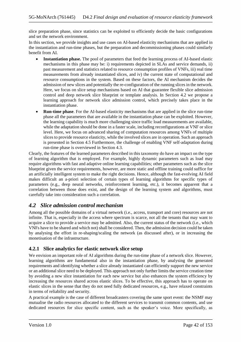
5G-MoNArch (761445) D4.2 Final design and evaluation of resource elasticity framework
Version 1.0 Page 42 of 153
slice preparation phase, since statistics can be exploited to efficiently decide the basic configurations
and set the network environment.
In this section, we provide insights and use cases on AI-based elasticity mechanisms that are applied in
the instantiation and run-time phases, but the preparation and decommissioning phases could similarly
benefit from AI.
• Instantiation phase. The pool of parameters that feed the learning process of AI-based elastic
mechanisms in this phase may be: i) requirements depicted in SLAs and service demands, ii)
past measurement and statistics related to resource consumption profiles of VNFs, iii) real time
measurements from already instantiated slices, and iv) the current state of computational and
resource consumptions in the system. Based on these factors, the AI mechanism decides the
admission of new slices and potentially the re-configuration of the running slices in the network.
Here, we focus on slice setup mechanisms based on AI that guarantee flexible slice admission
control and deep network slice blueprint or template analysis. In Section 4.2 we propose a
learning approach for network slice admission control, which precisely takes place in the
instantiation phase.
• Run-time phase. For the AI-based elasticity mechanisms that are applied in the slice run-time
phase all the parameters that are available in the instantiation phase can be exploited. However,
the learning capability is much more challenging since traffic load measurements are available,
while the adaptation should be done in a faster scale, including reconfigurations at VNF or slice
level. Here, we focus on advanced sharing of computation resources among VNFs of multiple
slices to provide resource elasticity, while the involved slices are in operation. Such an approach
is presented in Section 4.5 Furthermore, the challenge of enabling VNF self-adaptation during
run-time phase is overviewed in Section 4.3.
Clearly, the features of the learned parameters described in this taxonomy do have an impact on the type
of learning algorithm that is employed. For example, highly dynamic parameters such as load may
require algorithms with fast and adaptive online learning capabilities; other parameters such as the slice
blueprint given the service requirements, however, are more static and offline training could suffice for
an artificially intelligent system to make the right decisions. Hence, although the fast-evolving AI field
makes difficult an a-priori selection of certain types of learning algorithms for specific types of
parameters (e.g., deep neural networks, reinforcement learning, etc.), it becomes apparent that a
correlation between those does exist, and the design of the learning system and algorithms, must
carefully take into consideration such a correlation.
4.2 Slice admission control mechanism
Among all the possible domains of a virtual network (i.e., access, transport and core) resources are not
infinite. That is, especially in the access where spectrum is scarce, not all the tenants that may want to
acquire a slice to provide a service may be admitted. Also, the current status of the network (i.e., which
VNFs have to be shared and which not) shall be considered. Then, the admission decision could be taken
by analysing the effort in re-shaping/scaling the network (as discussed after), or in increasing the
monetisation of the infrastructure.
4.2.1 Slice analytics for elastic network slice setup
We envision an important role of AI algorithms during the run-time phase of a network slice. However,
learning algorithms are fundamental also in the instantiation phase, by analysing the generated
requirements and identifying whether a slice already instantiated can efficiently support the new service
or an additional slice need to be deployed. This approach not only further limits the service creation time
by avoiding a new slice instantiation for each new service but also enhances the system efficiency by
increasing the resources shared across elastic slices. To be effective, this approach has to operate on
elastic slices in the sense that they do not need fully dedicated resources, e.g., have relaxed constraints
in terms of reliability and security.
A practical example is the case of different broadcasters covering the same sport event: the NSMF may
mutualise the radio resources allocated to the different services to transmit common contents, and use
dedicated resources for slice specific content, such as the speaker’s voice. More specifically, as
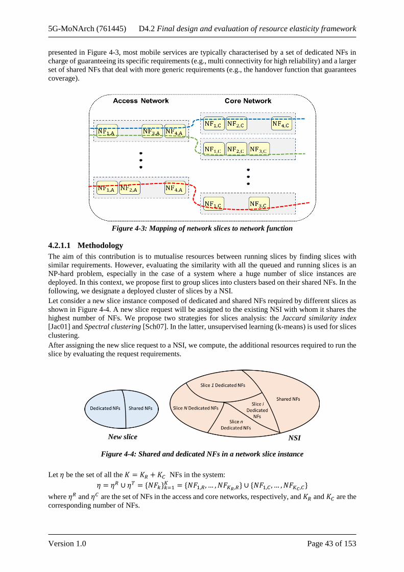
5G-MoNArch (761445) D4.2 Final design and evaluation of resource elasticity framework
Version 1.0 Page 43 of 153
presented in Figure 4-3, most mobile services are typically characterised by a set of dedicated NFs in
charge of guaranteeing its specific requirements (e.g., multi connectivity for high reliability) and a larger
set of shared NFs that deal with more generic requirements (e.g., the handover function that guarantees
coverage).
Figure 4-3: Mapping of network slices to network function
4.2.1.1 Methodology
The aim of this contribution is to mutualise resources between running slices by finding slices with
similar requirements. However, evaluating the similarity with all the queued and running slices is an
NP-hard problem, especially in the case of a system where a huge number of slice instances are
deployed. In this context, we propose first to group slices into clusters based on their shared NFs. In the
following, we designate a deployed cluster of slices by a NSI.
Let consider a new slice instance composed of dedicated and shared NFs required by different slices as
shown in Figure 4-4. A new slice request will be assigned to the existing NSI with whom it shares the
highest number of NFs. We propose two strategies for slices analysis: the Jaccard similarity index
[Jac01] and Spectral clustering [Sch07]. In the latter, unsupervised learning (k-means) is used for slices
clustering.
After assigning the new slice request to a NSI, we compute, the additional resources required to run the
slice by evaluating the request requirements.
Figure 4-4: Shared and dedicated NFs in a network slice instance
Let 𝜂 be the set of all the 𝐾 = 𝐾𝑅 + 𝐾𝐶 NFs in the system:
𝜂 = 𝜂𝑅 ∪ 𝜂𝑇 = {𝑁𝐹𝑘}𝑘=1𝐾 = {𝑁𝐹1,𝑅, … , 𝑁𝐹𝐾𝑅,𝑅} ∪ {𝑁𝐹1,𝐶 , … , 𝑁𝐹𝐾𝐶 ,𝐶}
where 𝜂𝑅 and 𝜂𝐶 are the set of NFs in the access and core networks, respectively, and 𝐾𝑅 and 𝐾𝐶 are the
corresponding number of NFs.
NSI New slice

5G-MoNArch (761445) D4.2 Final design and evaluation of resource elasticity framework
Version 1.0 Page 44 of 153
For the 𝑛𝑡ℎ slice request, we define the related slice blueprint by introducing the NF request 𝐷𝑛 and the
associated parameters 𝑋𝑛 as follows:
𝐷𝑛 = {𝑁𝐹𝑖∈𝐼}, 𝐼 ⊆ {1, . . , 𝐾}
𝑋𝑛 = {𝑋𝑖∈𝐼}, 𝐼 ⊆ {1, . . , 𝐾}
Then, we represent the NFs composing a request 𝐷𝑛 as a vector 𝜎𝑛 ∈ {0,1}𝐾 such as its 𝑗𝑡ℎ entry is
defined as:
𝜎𝑛𝑗= {
1 𝑖𝑓 𝑁𝐹𝑗 ∈ 𝐷, ∀𝑗 ∈ {1,⋯ , 𝐾}
0 𝑜𝑡ℎ𝑒𝑟𝑤𝑖𝑠𝑒
If 𝑁𝐹𝑖 ∈ 𝐷𝑛, i.e., the slice 𝑛 requests a certain NFs 𝑁𝐹𝑖, each of its parameters 𝑋𝑛,𝑖 is defined by 𝑏𝑖 binary labels:
𝑋𝑛,𝑖 = (𝑙𝑛,𝑖(1), 𝑙𝑛,𝑖(2),⋯ , 𝑙𝑛,𝑖(𝑏𝑖)), i ∈ I ⊆ {1, . . , 𝐾}.
For 𝑁𝐹𝑖 we map its parameters with the radio, computing, and storage resource requirements using a
model that includes a static part and a dynamic part, which depends on the NF parameters:
𝑑𝑟,𝑛,𝑖 = 𝜌𝑖 + 𝑓𝑟,𝑖 (𝑋𝑛,𝑖)
𝑑𝑐,𝑛,𝑖 = 𝜒𝑖 + 𝑓𝑐,𝑖 (𝑋𝑛,𝑖)
𝑑𝑚,𝑛,𝑖 = 𝜇𝑖 + 𝑓𝑚,𝑖 (𝑋𝑛,𝑖)
where 𝜌𝑖 𝜒𝑖, and 𝜇𝑖 are the minimum required resources for activating a given NF 𝑖, and 𝑓𝑟,𝑖 (𝑋𝑛,𝑖),
𝑓𝑐,𝑖 (𝑋𝑛,𝑖) and 𝑓𝑚,𝑖 (𝑋𝑛,𝑖) are the required resources as a function of NF's parameters 𝑋𝑛,𝑖. In summary,
the total resources demand of a slice request is presented as follows:
𝑇𝑛 = (∑𝑑𝑟,𝑛,𝑖𝑖∈ 𝐼
,∑𝑑𝑐,𝑛,𝑖𝑖∈ 𝐼
,∑𝑑𝑚,𝑛,𝑖𝑖∈ 𝐼
)
In the following, we present our slice clustering algorithms: the Jaccard similarity index and Spectral
clustering [Sch07].
Jaccard similarity-based assignment
The selection of the NSI is done by finding the NSI that shares the highest number of NFs with the slice
request and is able to support the additional resources required to support the new slice. For a better
understanding on how to assign a slice request to an NSI, let define the Jaccard similarity [Jac01] 𝑝𝑖,𝑗 as
the similarity between two subsets of NFs:
𝑝𝑖𝑗 =𝜎𝑖 ∩ 𝜎𝑗
𝜎𝑖 ∪ 𝜎𝑗
Accordingly, given a set of deployed NSI ℒ, where each NSI ℓ ∈ ℒ is characterised by a set of NFs
defined by𝜎ℓ, and the NFs in a slice request defined by 𝜎𝑛, the SA attempts to assign the slice request
to the NSI ℓ∗, such that
ℓ∗ = argmaxℓ∈ℒ 𝑝𝑛,ℓ
Spectral clustering-based assignment
Another strategy to optimise the resource usage, e.g., to enhance the slice performance or accepts new
requests, consists on re-clustering the running slices in new NSIs, in order to improve how the resource
are multiplexed across slices. Consider a set 𝑁 = {1,… ,𝑁} of running slices and their corresponding
NF requests {𝜎1, … , 𝜎𝑁}, we compute the adjacency matrix 𝐴, whose element 𝐴𝑛,𝑛′ = 𝑝𝑛𝑛′, if 𝑛 ≠ 𝑛′
and 𝐴𝑛,𝑛 = 0, represents the similarity in terms of required NFs of two running slices.
Then, the SA performs spectral clustering ([Lux07], [NJW02]) on the graph defined by 𝐴, and computes
the Laplacian's normalised eigenvectors and clusters the 𝑘 first eigenvectors using K-means [Jai10].
Intra-NSI Similarity for Resource Mutualisation
After assigning the new slice request into an NSI, we compute the additional resources required by
evaluating the request requirements using Cosine similarity.

5G-MoNArch (761445) D4.2 Final design and evaluation of resource elasticity framework
Version 1.0 Page 45 of 153
Let define the similarity index 𝑆 applied to the parameters 𝑋𝑛,𝑖 and 𝑋𝑛′,𝑖 of the NF 𝑖 shared by the slices
request 𝑛 and 𝑛′, is defined as follows:
𝑆(𝑋𝑛,𝑖, 𝑋𝑛′,𝑖) =∑𝑤𝑖,𝑗
𝐽
𝑗=1
ℎ(𝑙𝑛,𝑖(𝑗), 𝑙𝑛′,𝑖 (𝑗)),
where 𝐽 is the number of parameters of the NF 𝑖, 𝑤𝑖,𝑗 ∈ [0; 1] are weights that describe the relative
impact of each label on the resource request, with ∑ 𝑤𝑖,𝑗𝑗 , and ℎ is cosine similarity between two labels,
defined as:
ℎ (𝑙𝑛,𝑖(𝑗), 𝑙𝑛′,𝑖(𝑗)) =𝑙𝑛,𝑖(𝑗) ⋅ 𝑙𝑛′,𝑖(𝑗)
|𝑙𝑛,𝑖(𝑗)| |𝑙𝑛′,𝑖(𝑗)|
Considering all slices in the NSI, the maximum similarity achievable by the slice 𝑛 is obtained as
follows:
𝑠𝑛∗ = 𝑚𝑎𝑥∀ 𝑛′∈ 𝑁𝑆𝐼 𝑆(𝑋𝑛,𝑖, 𝑋𝑛′,𝑖),
the resources required for deploying the new slice 𝑛 in radio, computing, and storage, respectively, at a
NF 𝑖 are updated as follows:
𝑑𝑛,𝑟,𝑖′ = (1 − 𝑠𝑛
∗)𝑓𝑟 (𝑋𝑛,𝑖),
𝑑𝑛,𝑐,𝑖′ = (1 − 𝑠𝑛
∗)𝑓𝑐 (𝑋𝑛,𝑖),
𝑑𝑛,𝑚,𝑖′ = (1 − 𝑠𝑛
∗)𝑓𝑚 (𝑋𝑛,𝑖)
This approach can also be used as a congestion control mechanism to prevent resource outages: when
the system is close to saturate, the NSMF can re-cluster the overall set of services in new network slice
instances in order to maximise the resource usage. The latter could be implemented by using a spectral
clustering scheme [Sch07].
4.2.1.2 Main results
For simulation results, we use SARSA to learn admission control decisions. Figure 4-5 (Left) shows the
variation of resource usage as a function of slices departure probability in a system where the slice
requirements are computed without AI and compares these results with respect to the case where
unsupervised learning based on Jaccard similarity and spectral clustering are implemented. Spectral
clustering shows the best performance since it reformulates the slice clusters at each arrival or departure,
thus continuously optimising the shared resources at the cost of higher complexity. However, slices
dropping variation in Figure 4-5 (Right), shows that Jaccard similarity has the lowest dropping rate.
Spectral clustering shows the best trade-off between resource utilisation and slices dropping probability
when compared with SARSA without AI, and SARSA with Jaccard similarity.
Figure 4-5: Resource utilisation gains (Left) and slices dropping rates (Right) with AI-based
network slice setup

5G-MoNArch (761445) D4.2 Final design and evaluation of resource elasticity framework
Version 1.0 Page 46 of 153
Analysis with respect to the 5G-MoNArch KPIs
This study has a positive impact on both the slice minimum footprint and the system cost efficiency,
which are obviously inter-related. In fact, as shown in Figure 4-5 (left), our solutions (both Jaccard
similarity and the spectral clustering scheme) decrease the amount of required resources for a given
network load with respect to the baseline solution. This reduction in terms of minimum resource
footprint of a network slice decreases the probability that a slice request is dropped Figure 4-5 (Right),
and therefore improves the system cost efficiency, as the number of slice requests accepted in the system
increases.
4.2.2 A resource market-based admission control algorithm
In [BGB+17] a baseline for the design of a (market-based) admission control solution has been already
described using a Q-learning algorithm. However, we consider that solution cannot be applied to
practical scenarios, due to scalability limitation, so in this section we build on that Q-learning baseline
to design a new practical approach based on Neural Networks. In this section, we build on the Q-learning
baseline to design a practical approach based on Neural Network. The algorithm proposed is called
Network-slicing Neural Network Admission Control (N3AC). The main shortcomings of the Q-learning
approach of [BGB+17], which limit its applicability and need to be overcome in the design of a practical
solution, are due to the lack of scalability to larger space state. In particular:
• Q-learning based algorithms, including the one described in [BGB+17] need to store and update
the Q-values for each state-action pair. As a result, learning the right action for every state
becomes infeasible when the space state grows, since this requires visiting all the states multiple
times. This leads to extremely long convergence times that are unsuitable for most practical
applications.
• Storing and efficiently visiting the large number of states poses strong requirements on the
memory and computational footprint of the algorithm as the state space grows. In particular, the
number of states in our model increases exponentially with the number of network slicing
classes. Hence, when the number of network slicing classes grows, the computational resources
required rapidly become excessive.
A common technique to avoid that state space becomes too large is to generalise the experience learned
from some states by applying this knowledge to other similar states. The key idea behind
such generalisation is to exploit the knowledge obtained from a fraction of the space state to derive the
right action for other states with similar features. There are different generalisation strategies that can
be applied to Q-learning:
• The most straightforward technique is linear functions approximation. With this technique, each
state is given as a linear combination of functions that are representative of the system features.
These functions are then updated using standard regression techniques. While this approach is
scalable and computationally efficient, the right selection of the feature functions is a very hard
problem. In our scenario, the Q-values associated to states with similar features (e.g., the number
of inelastic users) are increasingly nonlinear as the system becomes larger. As a result,
linearisation does not provide a good performance in our case.
• A more powerful and flexible tool for generalisation with Q-learning are artificial Neural
Networks (NNs). NNs are a machine learning system consisting of simple, highly
interconnected elements called neurons that learn the statistical structure of the inputs if
correctly trained. With this tool, the design of neuron internals and the interconnection between
neurons are the most important design parameters.
Since NN can be applied to any scenario without making any assumption on the system and its inputs,
in this section we have used this technique to extend our learning algorithm to scale to larger systems.
4.2.2.1 Machine learning and neural networks framework
The fundamental building blocks of Neural Network (NN) based Machine Learning (ML) algorithms
are the following ones:
• A set of labelled data (i.e., system inputs for which the corresponding outputs are known) which
is used to train the NN (i.e., teach the network to approximate the features of the system).

5G-MoNArch (761445) D4.2 Final design and evaluation of resource elasticity framework
Version 1.0 Page 47 of 153
• A loss function that measures the neural network performance in terms of training error (i.e.,
the error made when approximating the known output with the given input).
• An optimisation procedure that reduces the loss functions at each iteration, making the NN
eventually converge.
Machine learning is usually categorised as supervised, unsupervised and reinforcement learning. A ML
system is supervised or unsupervised depending on whether the labelled data is available or not, and it
is a reinforcement learning system when it interacts with the environment receiving feedback from its
experiences.
NNs are a machine learning scheme that can be used for supervised/unsupervised learning and can be
integrated with reinforcement learning. In a NN we have multiple layers of interconnected neurons
organised as: (i) an input, (ii) an output and (iii) one or more hidden layers. A neuron is a non-linear
element that executes a so-called activation function to the linear combination of the weighted inputs.
Many different activation functions are available in the literature spanning from a linear function to
more complex ones such as Scaled Exponential Linear Unit (SELU), sigmoid or the Rectified Linear
Unit (ReLU).
In classical ML applications, the NN is trained using a labelled dataset: the NN is fed with the inputs
and the difference among the estimated output and the label is evaluated with the error function. Then,
the error is processed to adjust the NN weights and thus reduce the error in the next iteration. The weights
may be adjusted using a Gradient Descent approach: the measured error at the output layer is back-
propagated to the input layer changing the weights values of each layer accordingly.
One of the design choices that needs to be taken when devising a NN approach is the way neurons are
interconnected among them. The most common setup is feed-forward, where the neurons of a layer are
fully interconnected with the ones of the next. There are also other configurations, such as the
convolutional (where group of neurons are fully- connected with a smaller group of neurons in the next
layer) or the recurrent (where the output is used as input in the next iteration). Indeed, convolutional
networks are usually employed for image recognition, while recurrent are useful when the system input
and the output have a certain degree of mutual relation.
Furthermore, our NN design relies on a single hidden layer. Such a design choice is driven by the
following two observations: (i) it has been proven that is possible to approximate any function using
NN with a single hidden layer [HSW89] and (ii) while a larger number of hidden layers may improve
the accuracy of the NN, it also involves a higher complexity and longer training period; as a result, one
should employ the required number of hidden layers but avoid building a larger network than strictly
necessary.
Another crucial design decision for our NN framework is the integration with reinforcement learning,
which is needed in order to train the network without “ground truth” labelled data. To this end, we need
to design an algorithm that operates without any previously known output but getting more accurate
estimations of the output while exploring the system. This is a topic that has been extensively studied in
the literature [S+17]. In our framework, we devise a reinforcement learning approach by building on the
Q-learning algorithm described in [BGB+17]. We take as output values of the NN the Q-values defined
in our Q-learning algorithm, which correspond to the revenues received at a given state: the NN provides
estimates of the Q-value. Additionally, we measure the revenues obtained after taking a decision. Then,
the NN is trained by taking as error the difference between the current Q-value estimates and the
measured revenues.
The Q-values employed by our algorithm correspond to the revenues after accepting or rejecting a
request at a given state, respectively. In order to estimate these values, we rely on two different NNs:
one that provides an estimate of the revenue after accepting a request, and another one that provides the
estimate after rejecting it. When accepting a request, we evaluate the error of the corresponding NN,
and the same when rejecting a request. The main advantage of such an approach based on NN as
compared to Q-learning is that any decision serves to update the entire system and not just a specific Q-
value, and thus the learning phase can converge without needing to visit every single state several times.
One of the important aspects of the proposed framework is the memory footprint, which has a strong
impact on scalability. By using NNs, we do not need to keep track of the expected reward for each
individual state-action Q(s,a) any more, but we only store the weights of the NNs. As the number of

5G-MoNArch (761445) D4.2 Final design and evaluation of resource elasticity framework
Version 1.0 Page 48 of 153
weights is fixed by the NN layout, and it is usually much smaller than the total number of states, this
provides a much higher scalability, especially when the number of states explodes.
4.2.2.2 Algorithm description
In the following, we describe the proposed N3AC algorithm. This algorithm builds on the Neural
Networks framework described above, exploiting reinforcement learning to train the algorithm without
a ground truth sequence (the right sequence is not known a priori). The algorithm consists of four high-
level steps as described below. In addition to these steps, the algorithm relies on some cornerstone
procedures. N3AC leverages on the exploration-exploitation procedure to ensure that we cover the entire
space state during the exploration phase.
Step 1, acceptance decision
In order to decide whether to accept or reject an incoming request, we look at the Q-values resulting
from accepting and rejecting a request in the two NNs, respectively. Then, we take the decision that
leads to the higher Q-value. This procedure is used for elastic slices only, as inelastic slices shall always
be accepted as long as there is sufficient room. When there is no room for an additional slice, requests
are rejected automatically, regardless of their type.
Step 2, evaluation
By taking a decision in Step 1, the system experiences a transition from state s at step n, to state s′ at
step n +1. Once in step n +1, the algorithm has observed both the reward obtained during the
transition R(s,a) and a sample 𝑡𝑛 of the transition time. The algorithm trains the weights of the
corresponding NN based on the error between the expected reward of s estimated at step n and the target
value. This step relies on two cornerstone procedures:
• Step 2a, back-propagation: This procedure drives the weights update by propagating the error
measured back through all the NN layers and updating the weights according to their gradient.
The convergence time is driven by a learning rate parameter that is used in the weight updates.
• Step 2b, target creation: This procedure is needed to measure the accuracy of the NNs
estimations during the learning phase. At each iteration our algorithm computes the observed
revenue as follows:
o ω = R(s,a,s′)−σ𝑡𝑛+ max𝑎′
𝑄(s′,a′).
o As we do not have any real value to test the accuracy of the prediction, we also have to
estimate them. This is done by taking as error the difference between our estimated
revenue 𝑄𝑛+1 (s,a) given by the NN and the target given by the observed ω.
Step 3, penalisation
When a state in the boundary of the admissibility region is reached, the system is forced to reject the
request. In general, reaching these states should be avoided as it may lead to sub-optimal performance
(i.e., low revenues). To avoid this, a penalty is back-propagated for the actions that lead to such a
situation. In particular, (i) if the system reaches the full-occupation through a sequence of high-reward
actions, then the system is not penalised; and (ii) if it is reached through low-reward actions, then the
system is penalised and thus it learns to avoid poor decision sequences.
Step 4, learning finalisation
Once the learning phase is over, the NN training stops. At this point, at a given state we just take the
action that provides the highest expected reward.
4.2.2.3 Performance evaluation
In this section we evaluate the performance of the proposed algorithms via simulation. Unless otherwise
stated, we consider a scenario with four slice classes, two for elastic traffic and two for inelastic. We set
µ = 5 for all network slices classes, and the arrival rates equal to λi = 2µ and λe = 10λi for the elastic and
inelastic classes, respectively. We consider two network slice sizes, equal to C/10 and C/20, where C is
the total network capacity. Similarly, we set the throughput required guarantees for elastic and inelastic
traffic to Ri = Re = Cb/10. Two key parameters that will be employed throughout the performance
evaluation are ρe and ρi, the average revenue per time unit generated by elastic and inelastic slices,

5G-MoNArch (761445) D4.2 Final design and evaluation of resource elasticity framework
Version 1.0 Page 49 of 153
respectively (in particular, performance depends on the ratio between them). Following the N3AC
algorithm proposed in the previous section, we employ two feed-forward NNs, one for accepted requests
and another one for rejected. Each neuron applies a ReLU activation function, and we train them using
the NNs RMSprop algorithm implementation available in [Ker]. The output layers are composed of one
neuron, each of them applying a linear function.
Algorithm optimality
We first evaluate the performance of the N3AC algorithm (which includes a hidden layer of 20 neurons)
by comparing it against: (i) the benchmark provided by the optimal algorithm, (ii) the Q-learning
algorithm [BGB+17], and (iii) two naive policies that always admit elastic traffic requests and always
reject them, respectively. In order to evaluate the optimal algorithm and for Q-learning, we consider a
small scenario as these approaches do not scale to large scenarios. Figure 4-6 shows the relative average
reward obtained by each of these policies, taking as baseline the policy that always admit all network
slice requests (which is the most straightforward algorithm).
Figure 4-6: Revenue vs. ρi/ρe
We observe that N3AC performs very closely to the Q-learning and optimal policies, which validates
the proposed algorithm in terms of optimality. We further observe that the revenue improvements over
the naive policies is very substantial, up to 100% in some cases. As expected, for small ρi/ρe the policy
that always admits all requests is optimal: in this case both elastic and inelastic slices provide the same
revenue. In contrast, for very large ρi/ρe ratios the performance of the “always reject” policy improves,
as in this case the revenue obtained from elastic traffic is (comparatively) much smaller.
Learning time
One of the key advantages of the N3AC algorithm as compared with Q-learning is that it requires a
much shorter learning time. This is due to the fact that with N3AC the knowledge acquired at each step
is used to update the Q-values of all states, while with Q-learning we just update the Q-value of the state
being visited.
Figure 4-7: Learning time for N3AC and Q-learning

5G-MoNArch (761445) D4.2 Final design and evaluation of resource elasticity framework
Version 1.0 Page 50 of 153
To evaluate the gain provided by the NNs in terms of convergence time, we analyse the evolution of the
expected revenue over time for the N3AC and the Q-learning algorithms. The results are shown in Figure
4-7 as a function of the number of iterations. We observe that after few hundred iterations, N3AC has
already learned the correct policy and the revenue stabilises. In contrast, Q-learning needs several
thousands of iterations to converge. We conclude that N3AC can be applied to much more dynamic
scenarios as it can adapt to changing environments. Instead, Q-learning just works for static scenarios,
which limits its practical applicability. Furthermore, Q-learning, besides being more complex cannot
scale to large scenarios, as the learning time (and memory requirements) would grow unacceptably for
such scenarios.
Large scale scenario
The previous results have been obtained for a relatively small scenario where the evaluation of the
optimal and Q- learning algorithm was feasible. In this section, we assess the performance of the N3AC
algorithm in a large-scale scenario; indeed, one of the design goals of this algorithm is its scalability to
large scenarios. We consider a scenario with eight slice classes, four for elastic traffic and four for
inelastic. For each traffic type, we allow four network slice sizes, linearly distributed among C/10 and
C/20. We have the same throughput guarantees for elastic and inelastic traffic as in the previous
experiment (Ri = Re = Cb/10) and thus we have the same admissibility region (although the space state
is much larger now). We set µ and λ parameters in a way that the load of the network is similar to the
previous experiment. The NN is composed by 40 neurons in its hidden layer.
In this larger scenario, the optimal and Q-learning algorithms are not feasible, due to the larger number
of states. Hence, we evaluate the performance of N3AC and compare it against the naive policies only.
Figure 4-8 shows the relative average reward obtained by each of these policies, taking as baseline the
policy that always admits all network slice requests. Similarly, to the evaluation performed in the
previous experiment, we observe that the N3AC algorithm always substantially outperforms the naive
policies. As expected, for small ρi/ρe the policy that always admits all requests is optimal, while for very
large ρi/ρe ratios the performance of “always reject” policy improves since the revenue obtained from
the elastic traffic is much smaller.
Figure 4-8: Revenue vs. ρi/ρe
Analysis with respect to the 5G-MoNArch KPIs
This enabler is mainly focused to enhance the Cost efficiency KPI, by accepting or rejecting new
network slices instances requests with the goal of increasing the monetary efficiency per unit of resource
deployed. Results show that by applying this technique the relative venue is always optimal for small
scenarios and very high (compared to other techniques) for larger ones.
4.3 Intelligent VNF scaling and re-location
VNFs (especially the radio access ones) have very specific NFVI utilisation patterns. That is, according
to the user/service load, the VNF footprint on the virtual infrastructure may vary. Depending on the
requirements of the network slices they are in, as well as on the load of the cloud where they are running,

5G-MoNArch (761445) D4.2 Final design and evaluation of resource elasticity framework
Version 1.0 Page 51 of 153
they may need to be scaled up or out, in or down, or even migrated into a new location. In this field, ML
and AI algorithms may help to find the correct scaling strategy. More specifically, we tackle the first
problem in Section 4.3.1 and the second one in Section 4.3.2.
4.3.1 AI-assisted scaling and orchestration of NFs
With the explosion of artificial intelligence and virtualisation, and its applicability to communication
networks, the idea of self-governing networks has drawn the attention of the communications research
community. Works like [CZW+18] make use of Deep Double Q-learning (DDQ) and deep-SARSA
solutions for mobile edge computing. For VNF management, a proactive VM orchestration is proposed
in [TLZ+15] using Q-Learning. More recently, in [RAH+18], a machine learning classification problem
is formulated to decide the number of VNFs that must be deployed to meet the network traffic demands.
In this section, we formulate the problem of resource allocation for a central unit (CU) that deploys and
maintains a set of VNFs which serve the users of a distributed group of base stations. Using deep
deterministic policy gradient, i.e., deep neuronal networks as function approximation with the
deterministic policy gradient proposed as proposed in [SLH+14], an agent placed at the CU is trained to
learn to scale vertically (add CPU and Storage), horizontally (instantiate or stop containers) or offload
(send the task to the cloud) based on the system state (traffic arrival, services rates, SLAs...) and a
defined reward function (cost, delay, SLA, etc.). We use an actor-critic architecture with parameterised
action spaces, similarly to [HS16].
4.3.1.1 System model
In this work, we consider a radio access network (RAN), see Figure 4-9, consisting of a set of distributed
edge base stations (BSs), denoted by ℬ = {𝐵1, … , 𝐵𝐵}, connected to a local central unit (CU). Let 𝒩 ={𝑁1, … , 𝑁𝑁} define the set of distinct heterogeneous network’s services offered by the CU that can be
instantiated by any node in the network. Each 𝐵𝑖, ∀𝑖 ∈ [𝐵]1, according to its clients’ requirements,
instantiates a subset of VNFs taken from the set N, which are deployed and maintained by the CU. We
denote by 𝒩(𝑡) ⊂ 𝒩, the set of VNFs maintained by the CU during time interval t. For the sake of
simplicity, the time horizon is discretised into decision epochs, each of which is of equal duration T
(seconds) and is indexed by an integer 𝑡 ∈ ℕ+. The dependency on t of 𝒩(𝑡) emphasises the fact that,
overtime, VNFs can be added or removed from a BS provided services. In addition, the CU is connected
to a cloud data centre via a dedicated link of capacity 𝑅(𝑡) Mbps, with data capacity varying over time.
Figure 4-9: Considered system architecture
1 Notation: [K] denotes the set {1, … , 𝐾}.

5G-MoNArch (761445) D4.2 Final design and evaluation of resource elasticity framework
Version 1.0 Page 52 of 153
Furthermore, the CU has a local pool of resources that consists of a group of 𝐾 servers denoted by 𝒦 ={𝑆1, … , 𝑆𝐾} with a limited CPU and storage capability that can be used to instantiate VNF. We assume
homogeneity between servers, such that each 𝑆𝑘 , ∀𝑘 ∈ [𝐾] has the same storage size of 𝜂𝑚𝑎𝑥𝐵 bits and
a CPU of capability 𝜌𝑚𝑎𝑥𝐶 𝐻𝑧. Let us define 𝜂𝑘(𝑡)≤ 𝜂𝑚𝑎𝑥 and 𝜌𝑘
(𝑡)≤ 𝜌𝑚𝑎𝑥 as the storage and CPU,
being used at epoch 𝑡 at server 𝑆𝑘 respectively.
In this work we consider two main physical resources to be provisioned to the VNFs, CPU and storage,
and we consider that each network function Nj, ∀j ∈ [N], at epoch t uses ck, j(t)C Hz of CPU capability
and sk, j(t)B bits of storage, at a server Sk, k ∈ [K]. Where ck, j(t) ∈ [ck, jmin(t),ck, jmax(t)] and
sk, j(t) ∈ [sk, jmin(t),sk, jmax(t)]. Thus, a VNF has a different resource range in which it can operate
following the definition of an elastic network function, which is defined as a VNF that gracefully
degrades the QoS adapting it to the scarcity of resources. Each deployed VNF Nj, j ∈ [N], given the
service level agreement (SLA) has a minimum QoS that must always be ensured QoSjmin and a
maximum perceptible QoSjmax , which depends on the network resources allocated. The networks must
avoid violating the SLA and the actions taken, should be based on the fulfilling of the VNFs’ SLAs. Let
us define 𝐜𝑘,𝑗(𝑡)
and𝐬𝑘,𝑗(𝑡)
, as the total amount of CPU and storage, respectively, allocated to 𝑁𝑗 at 𝑆𝑘 during
epoch 𝑡.
If, due to network traffic fluctuation, the CU cannot cope with any new or existent VNF resource
requirements, i.e., ∑ ∑ 𝐜𝑘,𝑗(𝑡+1)
𝑘𝑗∈𝒩(𝑡+1) ⪆ 𝐾𝜌𝑚𝑎𝑥 or∑ ∑ 𝐬𝑘,𝑗(𝑡+1)
𝑘𝑗∈𝒩(𝑡+1) ⪆ 𝐾𝜂𝑚𝑎𝑥, or simply because
the CU finds it more appropriate, the VNF can be offloaded to the cloud. We assume a central cloud
data centre with an infinite capacity resource pool i.e., 𝜂𝑚𝑎𝑥𝑐𝑙𝑜𝑢𝑑 = 𝜌𝑚𝑎𝑥
𝑐𝑙𝑜𝑢𝑑 = ∞ and we do not consider
any resource penalty for a CU to relay the information needed to serve the customer/s to the cloud and
vice-versa. We define ��𝑘(𝑡) = [𝐜𝑘,1
(𝑡) , … , 𝐜𝑘,𝑁(𝑡) ] as the vector containing the amount of CPU allocated to
each VNF at server 𝑆𝑘 at epoch𝑡. Similarly, ��𝑘(𝑡)= [𝐬𝑘,1
(𝑡), … , 𝐬𝑘,𝑁
(𝑡)] denotes the vector containing the
amount of storage allocated to each VNF at server 𝑆𝑘 during epoch𝑡. Finally, we indicate by ��(𝑡) =
[��1(𝑡) , … , ��𝐾
(𝑡)] the vector of vectors, which accounts for the amount of CPU allocated to each VNF at
each server of CU during epoch 𝑡. In a similar fashion we specify by ��(𝑡) = [��1(𝑡), … , ��𝐾
(𝑡)] the vector of
vectors which accounts for the amount of storage allocated to each VNF at each server of the CU during
epoch 𝑡.
The service tasks generated by VNF 𝑁𝑗 , ∀𝑗 ∈ [𝑁] at 𝐵𝑖 across the time horizon 𝑡, form an independent
and identically distributed homogeneous Poisson point process with a common parameter 𝜆𝑖,𝑗(𝑡) ∈ [0,1],
and we consider that λi,j(t)
remains constant during each decision epoch t.
As soon as an arrival occurs, the CU needs to provision 𝑁𝑗 with the pertinent resources 𝑟𝑗 or offload this
function to the cloud data centre. The service times have an exponential distribution with rate parameter
𝜇𝑗 per customer, where 1/𝜇𝑗 is the expected service time of a customer of 𝑁𝑗 , ∀𝑗 ∈ [𝑁]2.
4.3.1.2 Problem formulation
Network sate space
The network state space defines the set of all possible configurations of the network. In the
aforementioned problem, the state space at the CU is given by:
• Arrival rates(𝜆𝑖,𝑗(𝑡)).
• VNFs deployed(𝒩(𝑡)).
• Cloud link capacity(𝑅(𝑡)).
• CPU load of each VNF at each server(��(𝑡)).
• Storage load of each VNF at each server of each VNF(��(𝑡)).
2 The technology that we envisage for virtualisation of network functions is Docker containers.

5G-MoNArch (761445) D4.2 Final design and evaluation of resource elasticity framework
Version 1.0 Page 53 of 153
So, the network state space at epoch 𝑡 is characterised by 𝒳(𝑡) = (𝜆𝑖,𝑗(𝑡),𝒩(𝑡), ��(𝑡) , ��(𝑡) , 𝑅(𝑡)) ∈ 𝒳.
Where
𝒳 = {× {ℝ+}𝑗∈𝒩, 𝑖∈ℬ} ×𝒩 × {× {0,… , 𝜌𝑚𝑎𝑥}𝑘∈𝒦} × {× {0,… , 𝜂𝑚𝑎𝑥}𝑘∈𝒦} × ℝ+.
Resource allocation actions
In our model, we consider three distinct ways of how a CU can react to the workload variations of the
exiting VNFs or to the deployment/s of new/s VNF/s, these are: vertical scaling, horizontal scaling and
work offloading.
Before explaining these actions, we define a Parameterised Action space Markov Decision Process
(PAMDP). We define the set of discrete actions as 𝒜𝐷 = {𝑎1, 𝑎2, … , 𝑎𝐷}, where each discrete action
𝑎 ∈ 𝒜𝑑 features 𝑛𝑎 discrete parameters {𝑝1𝑎, … , 𝑝𝑛𝑎
𝑎 } ∈ ℤ𝑛𝑎. Thus, the tuple (𝑎, 𝑝1𝑎 , … , 𝑝𝑛𝑎
𝑎 ) represents
an action, and the action space is given by 𝐴 =∪𝑎∈𝒜𝐷(𝑎, 𝑝1
𝑎 , … , 𝑝𝑛𝑎𝑎 ).
Vertical scaling
The vertical scaling action (𝒜𝑉) refers to the capacity of the CU to add or remove physical resources to
a deployed VNF. As mentioned before, in this work we focus on two main resources: CPU and storage.
Considering the traffic fluctuations and the 𝑟𝑗 requirements, a CU might decide to increase (decrease)
the CPU, the memory or both, of a deployed instance independently.
For each resource we define the vertical parameter set as follows,
{𝑝𝐶𝑃𝑈 = {𝑘 ⋅ 𝐵 ∣ 𝑘 ∈ ℤ, 0 ≤ 𝑘 ≤ 𝜌𝑚𝑎𝑥}
𝑝𝑆 = {𝑘 ⋅ 𝐶 ∣ 𝑘 ∈ ℤ, 0 ≤ 𝑘 ≤ 𝜂𝑚𝑎𝑥}.
Vertical scaling is limited by the resources of the physical server in which a container is deployed, thus,
the limitation of 𝜌𝑚𝑎𝑥 and 𝜂𝑚𝑎𝑥. The range of the parameters, from 0 to 𝐴𝑚𝑎𝑥 is discretised using the
step size 𝐵 for resource memory, and 𝐶 for CPU allocation.
Horizontal scaling
Horizontal scaling is the capability to connect multiple hardware or software entities, such as servers,
so that they work as a single logical unit. In our scenario, horizontal scaling refers to the deployment of
new containers to support an existing VNF or to live-migrate a VNF to another server. Every time a new
VNF is instantiated, a container is deployed in one of the 𝐾 servers and if for example, the workload of
a VNF increases, and the CU estimates that server 𝑘 at epoch 𝑡 + 1 will not be able to support its
operations, the CU might create another instance of the same VNF in another server, within its local
pool of resources. On the other hand, the CU might decide to move the whole VNF to another server,
i.e., live-migration.
We define the horizontal parameters set associated with the horizontal action 𝒜ℎ as
{𝑝ℎ ∈ 𝒮 = {𝑆1…𝑆𝐾}\𝑆𝑘𝑝ℎ,𝑙 ∈ {0,1}
Where 𝑆𝑘 is the server at which the VNF is already running and 𝑝ℎ,𝑙 = 0 specifies that a VNF is to be
live-migrated, while 𝑝ℎ,𝑙 = 1 means that a VNF is to be given a new instance on another server. On the
other hand, 𝑝ℎ defines at which server a VNF is to be deployed (𝑝ℎ,𝑙 = 1) or live migrated (𝑝ℎ,𝑙 = 0).
If a 𝑁𝑗 is not currently running on the CU, the only important parameter is 𝑝ℎ, which defines the server
at which the VNF is to be deployed.
Work offload
The CU might foresee that, by neither scaling vertically nor scaling horizontally, can cope with a traffic
fluctuation of the VNFs, so the CU might decide to offload any VNF to the cloud. We define the work
offloading parameters set associated with the offloading action 𝒜𝑜𝑓 as
𝑝𝑜𝑓 ∈ {∅, 1}.
We can see that the offloading action is a binary decision. Note that we use ∅ as the action where the
CU agent does not change the network status, i.e., ��(𝑡) = ��(𝑡+1) and ��(𝑡) = ��(𝑡+1).

5G-MoNArch (761445) D4.2 Final design and evaluation of resource elasticity framework
Version 1.0 Page 54 of 153
Parameterised action space
Following the PAMDP notation, in the formulated problem, the complete parameterised action space
for each virtual function is given by
𝒜 = (𝒜𝑣 , 𝑝𝐶𝑃𝑈, 𝑝𝑆) ∪ (𝒜ℎ , 𝑝ℎ , 𝑝ℎ,𝑙) ∪ (𝒜𝑜𝑓 , 𝑝𝑜𝑓).
Each of the aforementioned actions are mutually exclusive, meaning that the CU can choose to either
𝒜𝑣, 𝒜ℎ or 𝒜𝑜𝑓. The first decision the CU must take is to whether 𝒜𝑣, 𝒜ℎ or 𝒜𝑜𝑓. Then, the different
parameters associated with each action are selected. At the beginning of each decision epoch 𝑡, the base
station randomly selects a VNF currently running or to be deployed, then chooses whether to scale
vertically, horizontally, offloading or do nothing, and finally selects the parameters according to the
action selected. The agent repeats the process for all the VNFs.
4.3.1.3 Cost
The cost model implemented will drive the agent’s behaviour to select an action on detriment of another.
We consider three types of costs: latency, financial cost and service continuity.
Latency (𝜹𝑻)
The latency considers all the delays associated with the NFV management.
• VNF resizing: Resizing a VNF consists of varying the amount of CPU and storage previously
allocated. We consider that the CU incurs in a delay of 𝛿𝑟,𝑐 = 1 𝑚𝑠 per unit C of CPU
added/removed and 𝛿𝑟,𝑠 = 2 𝑚𝑠, per block of memory of size B added/removed.
• Deployment: We consider a boot-up time of 𝛿𝑑,𝑏 = 41𝑚𝑠 per container and a termination time,
to spare the resources, of 𝛿𝑑,𝑡 = 30𝑚𝑠.
• Live migration: The action of container migration accounts for the boot-up time and termination
time just specified, and the transferring of information. We approximate the live-migration
latency for 𝛿𝑚,𝑐 = 5𝑚𝑠/𝐶 per unit of CPU and 𝛿𝑚,𝑠 = 10𝑚𝑠/𝐵 per unit of storage.
• Offloading: The latency of offloading a VNF to the cloud is given by𝐬𝑘,𝑗/𝑅. We consider that,
after a VNF has been offloaded and in order to keep the service running, a continuous flow of
information between the cloud and CU is registered until the VNF is terminated. This
transmission and reception of information incurs in a total delay penalty of 𝛿𝑜𝑓 = 2𝛼𝐬𝑘,𝑗/𝑅
(𝛼 < 1) for the VNF offloaded.
Financial Cost (𝑪𝑻)
A price model that takes into account the economic implications of the network configuration is
developed.
• Resources cost (𝐶𝑟): Based on Amazon Web Services pricing [AWS18], we consider a cost of
𝐶𝑠 = $ 0.0052/(𝐵 ⋅ 𝑚𝑖𝑛) for storage and a price of 𝐶𝑝 = $ 0.0094/(𝐶 ⋅ 𝑚𝑖𝑛) for CPU usage.
• Server cost (𝐶𝑖): Every time a server is powered on, we consider a one-time payment of $ 0.05
plus a variable cost of $ 0.001/min.
• Cloud cost (𝐶𝑠): The cost of offloading a VNF to the cloud equals to a one-time payment of $
0.1 plus a rental payment of $ 0.002/min until the VNF is terminated.
Service Continuity (𝑺𝑻)
Every VNF is associated with a 𝑄𝑜𝑆, the failure to provision resources accordingly, might incur in
service disruption which degrades the 𝑄𝑜𝑆 provided. We define the service continuity cost as:
𝑆𝑇 = ∑ 𝛾𝑗1 (𝑄𝑜𝑆𝑗(𝑡+1) < 𝑄𝑜𝑆𝑗)
𝑗∈𝒩(𝑡+1)
Where 𝑄𝑜𝑆𝑗(𝑡)
is the perceived 𝑄𝑜𝑆 of Nj, 1(x) denotes the logical operator, being equal to 1 if the
condition x is true and 0 otherwise. 𝛾𝑗 is the penalty for not fulfilling 𝑄𝑜𝑆𝑗.
Total Cost
We define the immediate cost at epoch t that help us quantify the network experience as:
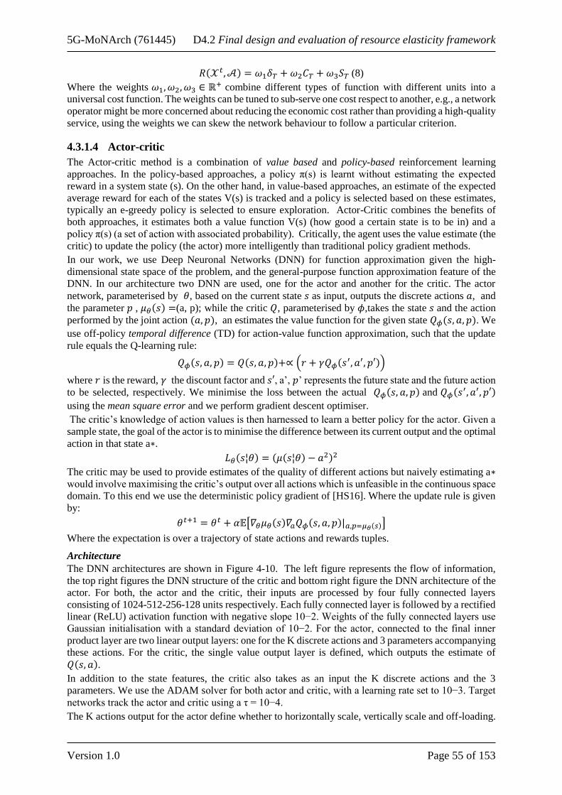
5G-MoNArch (761445) D4.2 Final design and evaluation of resource elasticity framework
Version 1.0 Page 55 of 153
𝑅(𝒳𝑡,𝒜) = 𝜔1𝛿𝑇 +𝜔2𝐶𝑇 +𝜔3𝑆𝑇 (8)
Where the weights 𝜔1, 𝜔2, 𝜔3 ∈ ℝ+ combine different types of function with different units into a
universal cost function. The weights can be tuned to sub-serve one cost respect to another, e.g., a network
operator might be more concerned about reducing the economic cost rather than providing a high-quality
service, using the weights we can skew the network behaviour to follow a particular criterion.
4.3.1.4 Actor-critic
The Actor-critic method is a combination of value based and policy-based reinforcement learning
approaches. In the policy-based approaches, a policy π(s) is learnt without estimating the expected
reward in a system state (s). On the other hand, in value-based approaches, an estimate of the expected
average reward for each of the states V(s) is tracked and a policy is selected based on these estimates,
typically an e-greedy policy is selected to ensure exploration. Actor-Critic combines the benefits of
both approaches, it estimates both a value function V(s) (how good a certain state is to be in) and a
policy π(s) (a set of action with associated probability). Critically, the agent uses the value estimate (the
critic) to update the policy (the actor) more intelligently than traditional policy gradient methods.
In our work, we use Deep Neuronal Networks (DNN) for function approximation given the high-
dimensional state space of the problem, and the general-purpose function approximation feature of the
DNN. In our architecture two DNN are used, one for the actor and another for the critic. The actor
network, parameterised by 𝜃, based on the current state 𝑠 as input, outputs the discrete actions 𝑎, and
the parameter 𝑝 , 𝜇𝜃(𝑠) =(a, p); while the critic 𝑄, parameterised by 𝜙,takes the state 𝑠 and the action
performed by the joint action (𝑎, 𝑝), an estimates the value function for the given state 𝑄𝜙(𝑠, 𝑎, 𝑝). We
use off-policy temporal difference (TD) for action-value function approximation, such that the update
rule equals the Q-learning rule:
𝑄𝜙(𝑠, 𝑎, 𝑝) = 𝑄(𝑠, 𝑎, 𝑝)+∝ (𝑟 + 𝛾𝑄𝜙(𝑠′, 𝑎′, 𝑝′))
where 𝑟 is the reward, 𝛾 the discount factor and 𝑠′, a’, 𝑝’ represents the future state and the future action
to be selected, respectively. We minimise the loss between the actual 𝑄𝜙(𝑠, 𝑎, 𝑝) and 𝑄𝜙(𝑠′, 𝑎′, 𝑝′)
using the mean square error and we perform gradient descent optimiser.
The critic’s knowledge of action values is then harnessed to learn a better policy for the actor. Given a
sample state, the goal of the actor is to minimise the difference between its current output and the optimal
action in that state a∗.
𝐿𝜃(𝑠¦𝜃) = (𝜇(𝑠¦𝜃) − 𝑎2)2
The critic may be used to provide estimates of the quality of different actions but naively estimating a∗ would involve maximising the critic’s output over all actions which is unfeasible in the continuous space
domain. To this end we use the deterministic policy gradient of [HS16]. Where the update rule is given
by:
𝜃𝑡+1 = 𝜃𝑡 + 𝛼𝔼[𝛻𝜃𝜇𝜃(𝑠)𝛻𝑎𝑄𝜙(𝑠, 𝑎, 𝑝)|𝑎,𝑝=𝜇𝜃(𝑠)]
Where the expectation is over a trajectory of state actions and rewards tuples.
Architecture
The DNN architectures are shown in Figure 4-10. The left figure represents the flow of information,
the top right figures the DNN structure of the critic and bottom right figure the DNN architecture of the
actor. For both, the actor and the critic, their inputs are processed by four fully connected layers
consisting of 1024-512-256-128 units respectively. Each fully connected layer is followed by a rectified
linear (ReLU) activation function with negative slope 10−2. Weights of the fully connected layers use
Gaussian initialisation with a standard deviation of 10−2. For the actor, connected to the final inner
product layer are two linear output layers: one for the K discrete actions and 3 parameters accompanying
these actions. For the critic, the single value output layer is defined, which outputs the estimate of
𝑄(𝑠, 𝑎).
In addition to the state features, the critic also takes as an input the K discrete actions and the 3
parameters. We use the ADAM solver for both actor and critic, with a learning rate set to 10−3. Target
networks track the actor and critic using a τ = 10−4.
The K actions output for the actor define whether to horizontally scale, vertically scale and off-loading.

5G-MoNArch (761445) D4.2 Final design and evaluation of resource elasticity framework
Version 1.0 Page 56 of 153
Figure 4-10: Actor-critic architecture
4.3.1.5 Numerical results
In this section we present the different results obtained with the Actor-Critic model just described above.
For the experimental setup we consider five possible different VNFs to be deployed in the network, with
the features of Table 4-1.
Table 4-1: VNF resource requirements
VNF CPU Storage 𝑸𝒐𝑺𝒋
𝒄𝟎 𝒄𝒓 𝒄𝒅 𝒔𝟎 𝒔𝒓 𝒔𝒅 𝑸𝒐𝑺𝒎𝒊𝒏 𝑸𝒐𝑺𝒎𝒂𝒙 𝜸
Firewall 40 30 20 60 70 30 31 60 4000
IDS 60 50 40 80 70 20 15 52 4000
VPN 40 40 10 40 40 10 17 45 4000
Call 10 50 10 10 40 10 32 65 4000
Video 80 20 5 100 20 10 40 95 4000
Furthermore, we consider a CU with 4 servers (𝐾 = 4) each of which has a maximum CPU of 400 C
𝐻𝑍 (𝜌𝑚𝑎𝑥 = 400) and storage capacity of 400 B bits (𝜂𝑚𝑎𝑥 = 400). The arrival rates (λi,j(t)
) for the
different VNFs at each epoch are sampled from a normal distribution, where each VNF’s Gaussian has
different mean and variance (see Table 4-2). The service rates at each decision epoch are also sampled
from a Gaussian distribution with the same parameters as its arrival rates but scaled by a factor of 0.4.
The parameters used to calculate the reward functions and that reinforce the actor behaviours are given
in Table 4-3.
Table 4-2: VNF Gaussian parameters for the arrival rates
VNF Mean Variance
Firewall 5 3
IDS 5 4
VPN 1 1
Call 9 3
Video 4 1
Table 4-3: Reward parameters
Delay (ms) 𝛿𝑟,𝑐= 3 𝛿𝑟,𝑠=4 𝛿𝑑,𝑏=20 𝛿𝑑,𝑡= 10 𝛼 =0.3
Cost (m$) 𝐶𝑟,𝑠=5 𝐶𝑟,𝑝=6 𝐶𝑖,𝑜 =2 𝐶𝑖,𝑣 =1 𝐶𝑐,0=1 𝐶𝑐,𝑣=3

5G-MoNArch (761445) D4.2 Final design and evaluation of resource elasticity framework
Version 1.0 Page 57 of 153
Once the system parameters are defined, we continue by providing the training results and a brief
discussion of them. Figure 4-11 shows the evolution of the average cost, as defined in Section 4.3.1.3,
over the distinct epochs. By epoch we mean every time the network weights are updated according to
the gradients calculated over a batch of samples.
Figure 4-11: Cost function evolution
As it can be seen in Figure 4-11, the agent at the beginning starts breaking the physics of the
environment, i.e., adding more CPU than the one available, trying to deploy a VNF in a server which
already has it running, which we penalise by a reward of -10.000. Once it has learnt the physics, the
agents start to learn the fulfilment of the SLA, because every time it’s violated we penalise by a reward
of – 4.000. As we can see, on the long run, the agent reward converges to the -800 zone, and neither the
SLA nor the physics of the environment are violated.
Furthermore, to improve exploration and avoid premature convergence to suboptimal deterministic
policies, we added the entropy of the policy π to the objective function. So, given the policy
parameterisation of 𝜋(𝑎/𝑠; 𝜃), the update rule is given by:
𝜃 ← 𝜃 + 𝛼∇𝜃 log 𝜋(𝑎𝑡/𝑠𝑡; 𝜃) (𝑅𝑡 − 𝑉(𝑆��)) + 𝛽∇𝜃𝐻(𝜋(𝑠𝑡; 𝜃))
The results obtained with this update rule are presented in Figure 4-12. As the figure shows, a faster
convergence rate and a lower cost are obtained. The model converges to an average cost of -150 in less
Epochs compared to the previous update.
Figure 4-12: Cost function evolution with entropy

5G-MoNArch (761445) D4.2 Final design and evaluation of resource elasticity framework
Version 1.0 Page 58 of 153
4.3.1.6 Mapping to KPIs
We now define three key performance indicators (KPIs) for MANO in 5G networks and then we map
the results obtained with the PAT algorithm to these KPIs.
The following KPIs are of interest for future 5G networks:
• Resource utilisation efficiency: Given the resources, CPU and storage, and a same number of
customers a resource utilisation efficiency is defined as the percentage of utilised resources
respect the total available resources for the execution of a VNF and a particular number of
customers. With the elastic functions employed in our model, the system should lead to a larger
resource utilisation efficiency, since it can shelter a higher number of customers over the same
physical infrastructure.
• Cost efficiency gain: This metric captures the average cost of deploying and maintaining the
network infrastructure to provide the required service to its users. Given the elastic nature of the
VNFs deployed, our CU system should be able to optimally dimension the network such that
less resources are required to support the same services; in addition, in lightly loaded scenarios
the elastic system should avoid the usage of unnecessary resources.
• Reliability: This KPI quantises the number of VNFs that can be allocated to the network edge,
and given the traffic fluctuations, not dropped/offloaded to the central cloud.
To be able to compare the proposed RL method performance, we implement a toy algorithm whose
function is the following: for each new customer, the algorithm checks whether the customer’s VNF is
already deployed in one of the servers. If so, computes the CPU and storage increment that the server
will need to allocate the user. If the server’s specifications allow for the deployment of the user, the user
is deployed. If not, another server is checked. If no server is able to coup with the new user, the user is
offloaded to the cloud.
Resource utilisation efficiency
A comparison of the resource utilisation between the toy algorithm and the AAC for the same traffic
pattern is presented in Figure 4-13. As it can be in the figure, the PAT algorithm clearly reduces the
average resource consumption of the CPU (significantly) and the storage.
Figure 4-13: Resource utilisation
Cost efficiency
A comparison of the resource monetary cost between the toy algorithm and the AAC for the same traffic
pattern is presented in Figure 4-14. As it can be seen in the figure, the ACC outperforms the toy example
in terms of cost saving, as less resources are used to allocate the same number of users.
Reliability
Figure 4-15 captures the number of VNFs offloaded to the central cloud given the traffic fluctuations.

5G-MoNArch (761445) D4.2 Final design and evaluation of resource elasticity framework
Version 1.0 Page 59 of 153
Figure 4-14: Monetary cost
Figure 4-15: Number of VNFs dropped
4.3.2 Dynamic VNF deployment
Whenever, resource scaling is not feasible, either because there are not enough available resources in
the used cloud to scale out, or because the VNF chain is characterised by low elasticity (i.e., stringent
resource requirements), re-locate (a part of) the chain is an interesting solution to meet the service
requirements.
Let us consider Centralised Radio Access Network (CRAN), where the Radio Access Network (RAN)
is composed by a set of Remote Radio Heads (RRHs) and supported by cloud infrastructure composed
by a central cloud and an edge cloud of computational capacity Cc and Ce [GFLOPS/s], respectively (see
Figure 4-16). We aim to study how this infrastructure can be used to deploy a set of network slices
S={1,2,…,S}, each one composed by a chain of Ns VNFs. A VNF is characterised by a specific
computational requirement, 𝜆s,n [GFLOPS], s 𝜖 S, n 𝜖 Ns:={1,2,…,Ns}. In the chain, each VNF n
receives inputs from the VNF n-1, passes its output to the VNF n+1, and potentially provides a feedback
to the VNF n-1, e.g., an acknowledgement or a negative acknowledgement. These interactions are
characterised by timing requirements that guarantee reliable operations in the service chain.
To maximise the system performance and the number of slices that can be deployed on the cloud
infrastructure, each chain can be split and its VNFs deployed in the most appropriate cloud, e.g., where
more computational resources are available. Moreover, multiple splits can be realised at each slice, to
increase the system flexibility. However, this procedure has to be carefully designed to consider the
limited computational resources and the latency introduced by the link between the central and the edge

5G-MoNArch (761445) D4.2 Final design and evaluation of resource elasticity framework
Version 1.0 Page 60 of 153
clouds, and between them and the access network. Specifically, the edge cloud capacity is typically
much lower than that of the central cloud, but the latter is characterised by a higher communication
latency as it is typically located in a remote area. In addition, VNFs related to lower layer functions,
e.g., signal processing, require low latency and high computational resources, which makes this process
even more challenging.
Liu et al. [LZG+15] proposed a graph-based model to investigate the trade-off between computational
and fronthauling costs when deciding the proper functional split. However, the authors consider cloud
units with unlimited capacity. Koutsopoulos studied the joint functional split selection and baseband
server scheduling problem in a CRAN [Kou17]. However, he considered only the overall service
latency, without considering the requirements of the specific VNFs. Alabbasi et al. have focused on a
hybrid CRAN architecture and they investigated the optimal functional split that jointly limits the system
power consumption and the bandwidth usage in the link between the edge and the central clouds
[AWC18]. The authors did not consider that each VNF has specific processing and latency requirements.
Figure 4-16: System model
Musumeci et al. [MBC+16] formulate an Integer Linear Programming (ILP) to investigate the problem
of finding the best deployment location for the VNF chain. However, they focus on the fronthaul
constraints, without considering the requirements of the network slice. Also, functional split is not
considered in this work. Arouk et al. investigate the deployment of network function in hybrid cloud
infrastructure [ANT17] [ATN+18]. They consider not only the overall latency constraint of the slice but
also the requirements of each VNF. However, they do not consider how the functional split affects the
computational resource requirements.
All these works consider slices with the same constraints; however, 5G systems need to comply with
services with heterogeneous requirements, which determine the computational and latency constraints
of each VNF chain.
4.3.2.1 Problem statement
The problem of minimising the amount of total computational resources required to run S slices by
jointly optimising the VNF deployment and the computational resource allocation can be formulated as
follows:
min{𝑅𝑠,𝑛𝑐 ,𝑅𝑠,𝑛
𝑒 ,𝑥𝑠,𝑛}∑ ∑ 𝑅𝑠,𝑛
𝑐 𝑥𝑠,𝑛 +
𝑛 𝜖 𝑁𝑠𝑠 𝜖 𝑆
𝑅𝑠,𝑛𝑒 (1 − 𝑥𝑠,𝑛)

5G-MoNArch (761445) D4.2 Final design and evaluation of resource elasticity framework
Version 1.0 Page 61 of 153
𝑠. 𝑡. 𝑥𝑠,𝑛 𝜖 {0,1}, ∀ 𝑠 𝜖 𝑆, 𝑛 𝜖 𝑁𝑠
∑ ∑ 𝑅𝑠,𝑛𝑐 𝑥𝑠,𝑛 ≤ 𝐶
𝑐
𝑛 𝜖 𝑁𝑠𝑠 𝜖 𝑆
∑ ∑ 𝑅𝑠,𝑛𝑒 (1 − 𝑥𝑠,𝑛) ≤ 𝐶
𝑒
𝑛 𝜖 𝑁𝑠𝑠 𝜖 𝑆
𝑙𝑠,𝑛𝑃 + 𝑓𝑠,𝑛
𝐶 ≤ 𝑓𝑠,𝑛 , ∀ 𝑠 𝜖 𝑆, 𝑛 𝜖 𝑁𝑠
𝑙𝑠,𝑛𝑃 + 𝑏𝑠,𝑛
𝐶 ≤ 𝑏𝑠,𝑛, ∀ 𝑠 𝜖 𝑆, 𝑛 𝜖 𝑁𝑠
where
• 𝑅𝑠,𝑛𝑐 and 𝑅𝑠,𝑛
𝑒 denote the amount of computational resources allocated by the central cloud and
the edge cloud to the VNF 𝑛 of the slice 𝑠.
• Moreover, 𝑥𝑠,𝑛 is a binary variable with 𝑥𝑠,𝑛=1 if the VNF 𝑛 is executed at the central cloud and
𝑥𝑠,𝑛=0 otherwise.
Here, the second and third equations above denote the resource allocation constraints at the central cloud
and edge cloud, respectively.
The constraints fourth and fifth equations above indicate that the sum of the processing latency related
to the VNF 𝑛 plus the latency to communicate its output to the neighbouring VNFs (𝑛 +1, 𝑛 -1) has to
be below specific latency constraints, i.e., 𝑓𝑠,𝑛 and 𝑏𝑠,𝑛 , respectively.
Furthermore, 𝑙𝑠,𝑛𝑃 describes the processing latency, which depends on the node where the VNF is
executed and the resources it receives, and it can be modelled as follows:
𝑙𝑠,𝑛𝑃 =
𝜆s,n𝑥𝑠,𝑛𝑅𝑠,𝑛𝑐 +
𝜆s,n(1 − 𝑥𝑠,𝑛)
𝑅𝑠,𝑛𝑒 .
The first term in above represents the processing latency if the VNF 𝑛 is executed in the central cloud
while the second term describes the processing latency if it runs in the edge cloud. Concerning the
communication latency, we assume it to be negligible when the related VNFs are located in the same
cloud. In contrast, when there is a split between 𝑛 and its neighboring VNFs 𝑛 -1, the associated latency
𝑏𝑠,𝑛𝐶 can computed as follows:
𝑏𝑠,𝑛𝐶 = {
𝑑𝑒,𝑐𝑣(𝑥𝑠,𝑛(1 − 𝑥𝑠,𝑛−1) + 𝑥𝑠,𝑛−1(1 − 𝑥𝑠,𝑛)), ∀ 𝑛 𝜖 𝑁𝑠\{1}
1
𝑣(𝑥𝑠,𝑛𝑑𝑐 + 𝑑𝑒(1 − 𝑥𝑠,𝑛)) , 𝑛 = 1
,
where 𝑑𝑒,𝑐, 𝑑𝑒, and 𝑑𝑐 denote respectively the distances between the edge and the cloud nodes, between
the edge and the access network, and between the central cloud and the access network. Moreover, 𝑣 is
the speed of the fiber link (200 m/µs) used to connect them.
The first case in the above equation describes the communication delay for 𝑛 𝜖 𝑁𝑠\{1}, when either n is
the central cloud and n-1 is in the edge cloud or n is the edge cloud and n-1 is in the central cloud. The
second case describes the communication latency of the VNF 1 with respect to the network functions
that cannot be virtualised, (i.e., the Radio Frequency functions implemented in the RRHs). This latency
depends on whether the VNF 1 runs at the central cloud or at the edge unit.
Moreover, when there is a split between 𝑛 and its neighboring VNFs n+1, the communication delay 𝑓𝑠,𝑛𝐶
can computed as follows:
𝑓𝑠,𝑛𝐶 = {
𝑑𝑒,𝑐𝑣(𝑥𝑠,𝑛(1 − 𝑥𝑠,𝑛+1) + 𝑥𝑠,𝑛+1(1 − 𝑥𝑠,𝑛)), ∀ 𝑛 𝜖 𝑁𝑠\{Ns}
0, 𝑛 = Ns
,
The first case in the equation above describes the communication delay for 𝑛 𝜖 𝑁𝑠\{Ns}, when either 𝑛
is the central cloud and 𝑛+1 is in the edge cloud or n is the edge cloud and n+1 is in the central cloud.

5G-MoNArch (761445) D4.2 Final design and evaluation of resource elasticity framework
Version 1.0 Page 62 of 153
The second case indicates that there is no communication latency related to the VNF Ns with respect to
a following VNF as it is last VNF in the slide. Therefore, the constraint 𝑓𝑠,𝑛 is only related to the
computational latency associated to Ns.
The overall optimisation problem is thus not easy to solve since 1) it is a mixed-integer problem and 2)
it has non-convex constraints due to the coupling within binary variables.
4.3.2.2 Problem reformulation
The optimisation problem above can be reformulated as an integer linear programming (ILP) by deriving
the computational resources needed to satisfy each VNF computational and latency constraints, by fixing
the cloud node selection as described in [DLY19].
min{,𝑥𝑠,𝑛}
∑ ∑ ��𝑠,𝑛𝑐 +
𝑛 𝜖 𝑁𝑠𝑠 𝜖 𝑆
��𝑠,𝑛𝑒
𝑠. 𝑡. 𝑥𝑠,𝑛 𝜖 {0,1}, 𝑠 𝜖 𝑆, 𝑛 𝜖 𝑁𝑠
∑ ∑ ��𝑠,𝑛𝑐
𝑛 𝜖 𝑁𝑠𝑠 𝜖 𝑆
≤ C𝑐 ,
∑ ∑ ��𝑠,𝑛𝑒
𝑛 𝜖 𝑁𝑠𝑠 𝜖 𝑆
≤ C𝑒 ,
𝑑𝑒,𝑐|𝑥𝑠,𝑛 − 𝑥𝑠,𝑛+1| ≤ 𝑣𝑓𝑠,𝑛, 𝑠 𝜖 𝑆, 𝑛 𝜖 𝑁𝑠\{Ns}
𝑑𝑒,𝑐|𝑥𝑠,𝑛 − 𝑥𝑠,𝑛−1| ≤ 𝑣𝑏𝑠,𝑛, 𝑠 𝜖 𝑆, 𝑛 𝜖 𝑁𝑠\{1}
𝑑𝑐𝑥𝑠,1 + 𝑑𝑒(1 − 𝑥𝑠,1) ≤ 𝑣𝑏𝑠,1, 𝑠 𝜖 𝑆
This new problem can be optimally solved through numerical solvers. Although this new problem is
equivalent to the original problem, it can be more efficiently solved. First, as we have explicitly
computed the optimal resource allocation variables, the above problem is characterised by one third of
the variables of the original problem. In addition, by reformulating the latency constraints as
computational resource ones, we have characterised the coupling within the binary variables through
new relations, which can be efficiently linearised.
Extension to the multiple-edge cloud case
We now analyse the optimal VNF deployment in a hybrid cloud infrastructure composed of multiple
edge clouds and one central cloud. In this case, depending on the resource availability and network
constraints, each VNF can be deployed either at the central cloud or at one of the multiple edge clouds.
We use 𝐾 = {0,1,2,⋯ , K} to denote the set of nodes in the hybrid cloud infrastructure each of
computational capacity C𝑘; then, we define a new VNF association variable as 𝑥𝑠,𝑛𝑘 such that 𝑥𝑠,𝑛
𝑘 = 1
if VNF 𝑛 𝜖 𝑁𝑠 of the slice 𝑠 𝜖 𝑆 is associated with cloud node 𝑘 𝜖 𝐾 and 𝑥𝑠,𝑛𝑘 = 0 otherwise. The new
problem above can thus be reformulated again as an integer linear programming (ILP) as follows:
min{,𝑥𝑠,𝑛
𝑘 }∑ ∑ ∑ ��𝑠,𝑛
𝑘
𝑛 𝜖 𝑁𝑠𝑠 𝜖 𝑆 k 𝜖 𝐾
𝑠. 𝑡. 𝑥𝑠,𝑛𝑘 𝜖 {0,1}, k 𝜖 𝐾, 𝑠 𝜖 𝑆, 𝑛 𝜖 𝑁𝑠
∑ ∑ ∑ ��𝑠,𝑛𝑘
𝑛 𝜖 𝑁𝑠𝑠 𝜖 𝑆 k 𝜖 𝐾
≤ C𝑘 ,
𝑑𝑘,𝑗max {∆𝑥𝑠,𝑛(𝑘,𝑗)+
, 0} ≤ 𝑣𝑓𝑠,𝑛, 𝑠 𝜖 𝑆, 𝑛 𝜖 𝑁𝑠\{Ns}, k ≠ j 𝜖 𝐾
𝑑𝑘,𝑗max {∆𝑥𝑠,𝑛(𝑘,𝑗)−
, 0} ≤ 𝑣𝑏𝑠,𝑛, 𝑠 𝜖 𝑆, 𝑛 𝜖 𝑁𝑠\{1}, k ≠ j 𝜖 𝐾
𝑑𝑘𝑥𝑠,1𝑘 ≤ 𝑣𝑏𝑠,1, 𝑠 𝜖 𝑆, k 𝜖 𝐾

5G-MoNArch (761445) D4.2 Final design and evaluation of resource elasticity framework
Version 1.0 Page 63 of 153
∑ 𝑥𝑠,𝑛𝑘
k 𝜖 𝐾
≤ 1, 𝑠 𝜖 𝑆, 𝑛 𝜖 𝑁𝑠 ,
Where the third equation in the problem above ensures that each VNF is effectively deployed at one and
only one of the clouds in the hybrid infrastructure, 𝑑𝑘,𝑗 is the distance between nodes k ≠ j 𝜖 𝐾, and
∆𝑥𝑠,𝑛(𝑘,𝑗)+
and ∆𝑥𝑠,𝑛(𝑘,𝑗)−
denote the additional rates, required by VNF 𝑛 𝜖 𝑁𝑠 deployed at cloud k 𝜖 𝐾 when
VNF 𝑛 + 1 and VNF 𝑛 − 1 are at cloud j ≠ k, respectively. The above problem is still an ILP, although
it is more complex than the first reformulated problem, mainly due to the higher number of variables.
Accordingly, to find efficient slice deployment solutions in scenarios with a large set of slices and/or
clouds, we propose a low-complexity heuristic based on the special structure the latest version of the
optimisation problem.
More specifically, the proposed heuristic is based on the finding that deploying a full chain in a single
cloud likely lowers the computational rate required by the slice, as it does not introduce any
communication delay in the VNF chain. In addition, we take advantage of the similarity of our ILP with
the so-called bin packing problem, and thus we use in the proposed heuristic a best fit decreasing strategy
[MT+90], whose performance are known to be relatively close to the optimal one for the offline bin
packing. In the best fit decreasing strategy, the best fit for a new request is the feasible cloud with the
smallest available computational capacity (which is likely to be an edge cloud), to limit the amount of
resources which may be left unused. Moreover, since dealing with larger computational requests is more
difficult, the best fit decreasing scheme sorts the requests in a descending order and attempts to place
the slice with the largest computational request first. The proposed ‘Best Fit with IteRative Split Trial’
(B-FIRST) strategy manages one slice request at each iteration; when there is no cloud with sufficient
computational resources to deploy the overall slice chain, the algorithm selects, within the functional
split options, the one that enables to accept the slice request with minimum additional computational
resources. When a feasible split does not exist, or the slice request can be fulfilled, the algorithm attempts
to deploy the second most demanding slice, and so on. The algorithm terminates when all slice chains
have been tested.
4.3.2.3 Simulation results
In this section, we focus on a simple cloud infrastructure composed by a central cloud and a single edge
cloud. The goal is twofold: first, we aim to assess the advantage of the hybrid architecture with respect
to a more classic solution based on a central cloud; then, we target to highlight the advantage of our
optimal VNF chain deployment scheme over less flexible solutions. To solve the first ILP optimisation
problem, we use Gurobi [Gurobi2018], which uses a branch-and-cut algorithm for ILP problems.
Figure 4-17 shows the resource utilisation gain provided by the usage of a hybrid cloud infrastructure
with respect to a classical CRAN architecture, as a function of the required VNF chains and for different
distances of the central cloud from the central macro cell. In this simulation, we focus on the optimal
deployment of chains related to a single service (eMBB), in order to clearly evaluate the advantages of
the hybrid architecture over the CRAN approach.
We set the cloud computational capacity Cc equal to 13440 GFLOPS/s in the central cloud only
architecture; in the hybrid solution, the central cloud has two third of the overall capacity, i.e., 8960
GFLOPS/s, while the rest is available at the edge cloud, i.e., Ce=4480 GFLOPS/s. First, we can note
that, as expected, the larger the distance of the central cloud from the access network, the larger the gain
of the hybrid infrastructure. When the distance is equal to 30 km, having an edge cloud leads to limited
gain as the hybrid infrastructure requires only 5% less of the computational resources needed by the
central cloud; however, up to 17 % and 43 % gains are measured when the central cloud is located at 90
and 150 km from the access network. For a given distance, the experienced gain slowly decreases when
the number of chains to be deployed increases when the number of chains is low; then, beyond a given
number of chain (16 in these results), which depends on the edge cloud capacity, the edge cloud starts
to saturate and the central cloud is used also in the hybrid infrastructure, which notably decreases the
resource utilisation gain. Finally, it is worth to notice, that the gain provided by hybrid cloud
infrastructure pave the way for a larger number of chains that can be accepted for a fixed value of
computational capacity. In fact, although the CRAN solution accepts up to 38 and 27 chains when the

5G-MoNArch (761445) D4.2 Final design and evaluation of resource elasticity framework
Version 1.0 Page 64 of 153
central cloud is located at 90 and 150 km, in the same condition, the hybrid infrastructure enables to
serve up to 42 and 39 chains, which correspond to a gain of 11 % and 44 %, respectively.
Figure 4-17: Resource utilisation gain of a hybrid cloud infrastructure over a CRAN solution with
respect to the number of required eMBB VNF chains
In Figure 4-18 we show the computational resources required by the hybrid infrastructure, when using
different VNF deployment schemes, as a function of the number of VNF chains. In this case, we consider
a mix of VNF chains, related to massive Machine Type Communication (mMTC), eMMB, and two
ultra-reliable low latency communication (URLLC) services. We compare the performance of the
optimal deployment scheme with two simple solutions denoted as fixed split and fixed service. In the
fixed split solution, the VNF of each chain, independently of the type of service, are split in the same
manner. Specifically, the VNFs up to the lower Medium Access Control (MAC) (see Figure 4-19) are
deployed in the edge cloud, while the other VNFs are instantiated in the central cloud. In contrast, in the
fixed service scheme, the mMTC, eMBB, and URLLC 1 chains are always deployed at the central cloud,
while only the URLLC 2 chains (which has the hardest latency constraints) are allotted to the edge cloud.
Dashed, solid, and dotted-dashed lines respectively represent the optimal solution, the fixed service
scheme, and the fixed split approach. Moreover, circle marked, cross marked, and square marked lines
describe the performance when the central cloud is located at 30, 60, and 90 km from the edge cloud.
First of all, we can notice as the computational resource usage increases with the number of accepted
chains. The larger increase in the resource usage corresponds to the chains 3, 6, and 9, which are related
to the URLCC 1 service that has the largest bandwidth requirements and low latency constraints. Also,
we can observe as proposed optimal scheme greatly enhances the number of chains that can be
successfully deployed with the two static solutions, even when the central cloud is located nearby the
edge cloud (and the macro cell network). In fact, for several problem instances, the static schemes fail
to find a feasible solution, in contrast to the optimal deployment approach.
Specifically, for de,c= 30 km, the optimal solution provides up 11 VNF chains, while the fixed service
and the fixed split achieves up to 8 and 5 chains, with a gain of 37.5% and 120% in term of number of
deployed services. These gains further increase when the distance between the central cloud and the
edge cloud augments: the optimal solution leads to a 266% gain with respect to both the two static
schemes in terms of served chains when de,c=60 km. Moreover, when de,c= 90 km, it gains up to 166%
and 300%, with respect to the fixed service and the fixed split schemes.

5G-MoNArch (761445) D4.2 Final design and evaluation of resource elasticity framework
Version 1.0 Page 65 of 153
Figure 4-18: Resource utilisation of the different VNF chain deployment schemes with respect to
the number of required VNF chains; Cc=8960 GFLOPS/s and Ce=4480 GFLOPS/s
However, when fixing the number of chains, the measurable gain in term of resource usage of the
optimal solution with fixed service and the fixed split schemes are lower: up to 5% and 10% for de,c=30
km and up to 11% and 19% for de,c=60 km. For de,c=90, we measure up to 41% gain with respect to the
fixed service scheme; however, we cannot measure appreciable gains with respect to the fixed split
scheme, since it fails to deploy more than two chains due to the large distance between the two clouds.
Overall, we can observe that when the number of VNF chains (or equivalently de,c) increases, the
proposed scheme brings the required flexibility to balance the cloud load (i.e., moving VNFs from one
cloud to another) to make computational resources available for the chains with more stringent
requirements. In contrast, the static schemes lack such flexibility and lead to limit performance.
In the future studies, we will focus on learning how the slice requirements change during time, in order
to proactively move the VNFs from one cloud to another, and avoid service outages, as well to provide
efficient solutions when the number of variables is large.
Figure 4-19: 3GPP functional splits [3GPP17-38801]
Multi-cloud hybrid infrastructure
In this section we analyse the performance of the optimal scheme for deploying VNF chains when each
macro cell of the network is equipped with an edge cloud node. Figure 4-20 describes the computational
rates required by the optimal solution and the proposed B-FIRST heuristic with respect to the number
of VNF chains. We assume here that the edge clouds and the central cloud have a computational capacity
equal to 2240 GFLOPS/s and 8960 GFLOPS/s, respectively. Solid and dashed lines correspond to the

5G-MoNArch (761445) D4.2 Final design and evaluation of resource elasticity framework
Version 1.0 Page 66 of 153
performance of the optimal solution and the heuristic scheme, respectively. Moreover, circle marked,
plus marked, and cross marked lines correspond respectively to the cases where the central cloud is 30,
60, and 90 km far from the central macro cell.
Figure 4-20: Overall computational rates required by the optimal solution and the proposed
heuristic B-FIRST as a function of the number of accepted VNF chains. Cc=8960 GFLOPS/s and
Ce=2240 GFLOPS/s.
First, we can notice that, when the central cloud distance is not large (i.e., 60 km and below) and the
number of required VNF chains is limited (up to 8), the performance of the heuristic and the optimal
scheme is very close; in fact, in this case, both the optimal and the heuristic schemes deploy as many
VNF chains as possible at the edge clouds, and when a VNF chain has to be deployed at the central
cloud, the additional computational rate required in the system is limited. However, when the central
cloud is located at 90 km from the macro cell, even for a small number of VNF chains (i.e., 3 to 5), the
optimal solution improves of 56% the computational resource efficiency with respect to the proposed
heuristic. In fact, in this case it is necessary to properly select the VNFs to deploy at the central cloud,
as those with stringent latency constraints will require a large amount of additional computational
resources to compensate for the communication delay introduced by the central cloud.
We now consider the case where the edge cloud capacity is larger and is set to be 4480 GFLOPS/s. In
contrast to the previous results, the optimal and the heuristic approaches have very similar performance,
even when the central cloud is located at the largest considered distance. As we show in the zoomed plot
inside Figure 4-21, the two approaches have the same trend until the system comes very close to the
saturation. In fact, a resource utilisation gain is appreciable, i.e., 10%, only when the central cloud is
located at a distance of 90 km from the central macro cell and the number of VNF requests is larger than
23. In the scenarios shown in Figure 4-21, there is less need for flexibility and complexity as the edge
clouds are well dimensioned to satisfy large computational requests, such as those related to the URLLC
services, and the proposed heuristic can be used as efficient solution for the VNF deployment in hybrid
cloud infrastructures. This result highlights the need for investigating an optimal size design in terms of
computational capacity of both central and edge clouds to serve heterogeneous slices with a limited
complexity.

5G-MoNArch (761445) D4.2 Final design and evaluation of resource elasticity framework
Version 1.0 Page 67 of 153
Figure 4-21: Overall computational rates required by the optimal solution and the proposed
heuristic B-FIRST as a function of the number of accepted VNF chains. Cc=8960 GFLOPS/s and
Ce=4480 GFLOPS/s.
Analysis with respect to the 5G-MoNArch KPIs
This study has a positive impact on both the system rescuability and reliability. From the one hand, it
provides the ability of overcoming a resource outage in a specific cloud by moving a VNF in another
cloud where enough resources are available. From the other hand, by enabling dynamic VNF
deployment, the system increases the percentage of time in which a VNF provides optimal operations.
However, these advantages lead to a higher slice resource footprint as moving slices far away from the
RAN or introducing split in the VNF chain increases the computational rate demanded by a slice.
4.4 Multi-objective resource orchestration
Multi-Objective (MO) optimisation has been shown to be effective in fields such as economics,
engineering and multi-modal analysis [KDT14]. Additionally, it has been used to efficiently solve 5G
specific problems such as energy efficient handing of base stations [FGY+17], VNF orchestration and
chaining [CZA+17], network deployment [TCS+15] and resource orchestration in network settings
without elasticity enabled [BJD+14], [BPL18], [XLY18]. This suggests that its use for the problem of
slice-aware resource allocation in mobile networks is promising.
Tackling inter-slice resource allocation problems in the context of elasticity enabled 5G mobile network
systems has been a topic that has garnered a lot of attention from both academics and businesses.
Researchers tend to focus on optimising resource allocation based on a single objective e.g. [SCC17],
[ZLC+17] or two objectives e.g. [WFT+18] or optimisation of more objectives but not a simultaneous
manner [PDD+17]. Moreover, the majority of the existing literature concentrates on modelling and
optimising radio resources e.g. data rate, physical resource blocks, Signal-to-Interference-plus-Noise-
Ratio (SINR), base station energy consumption etc., while not considering the resources required by the
virtualised parts of the network. [HLS18] offer a resource allocation process that could be extended to
include such resources and in [DSM+18] such resources are modelled in a generic manner, but no
solving process is offered. [SCC17] and [ZLC+17] study the optimisation of slice resource capacity,
[DSM+18] and [BRH+18] study profit maximisation in conjunction with resource utilisation efficiency.
In the following section results of a MO approach are presented, based on the problem formulation
presented on [5GM-D41]. Optimising the value of a single KPI, which could result to undesirable effects
with respect to the values of other KPI. Instead the solutions investigated satisfy the KPI objectives
without being dominated by other solutions, i.e. none of the values of the objective functions examined

5G-MoNArch (761445) D4.2 Final design and evaluation of resource elasticity framework
Version 1.0 Page 68 of 153
can be improved in value without the value of some other objective deteriorating. This results in a set
of optimal trade-off solutions between multiple KPIs, a non-trivial problem since there is no single
solution that simultaneously optimises each KPI.
4.4.1 Resource allocation approach based on MOEA/D
The first step of the proposed approach is the identification of the available physical resources and the
formulation of the shared resource pool that will be used for serving the slices. The available pool P
includes both network (e.g. bandwidth) and computational (e.g. CPU, memory) resources, located on
either the edge or the central cloud. . The entirety of the network and computational resources is noted
as:
P={r1,r2,…,r|P|}
Each slice corresponds to a service offered by the network, e.g., Virtual Reality (VR) or mobile
browsing.
Afterwards, the total demand per slice is defined as follows: Given the set of slices 𝑆 = 𝑠1, . . , 𝑠𝑖, the set
of time periods 𝑇 = 𝑡1, . . , 𝑡|𝑇|, and the set of user service requests Uqsi={u1si,u2si ,...,u|U|si}, define as
𝐷𝑠𝑖𝑡𝑘 the vector that represents the list of requests that wait in the execution queue of slice 𝑠𝑖 at time tk.
The order of the requests in this vector represents their priority in the queue:
Dsitk=[um,…,un]
For each slice, the combined total of requests, requires an amount of resources in order to be served
Esi={e1si ,e2si,...,e|E|si} with E being a subset of the available resources set P, E ⊆ P. Not all requests can
be accommodated, so for each request uj ∈ Uqsi per slice s ∈ Si, function xuj,SI is defined, where:
xuj,Si= {
1,if request uj for slice Si can be accommodated,
0,if not
The next step includes defining of the objective metric for the optimisation procedure. The resource
allocation problem is formulated as a minimisation problem, with respect to minimising a list of KPIs
of interest, e.g. latency, energy consumption etc. Since the resource allocation procedure can optimise
for either a single or multiple KPIs each time, the set of minimisation objectives is defined as:
J={J1,..J|J|}≡{KPI1,...,KPI|J|}
where each Ji represents a specific KPI, i.e. KPIi.
The desired result of the algorithm is the definition of a mapping function f: P×Dsitk→𝒫(P), for all
tk∈T,si∈S, and 𝒫(P) is the powerset of P. In other words, given the demand Dsitk and the available
resources P, function f returns a list of resources allocated to slice sj at time 𝑡𝑖, while also minimising
the list of objectives J. In this respect, the actual values of the KPIs utilised in set J depends on the
selection of the mapping function f, i.e. J is a function of f: J(f). Finally, the algorithm allocates the
required computational resources as follows:
arg minf J(f) subject to KPIJmin≤KPIJ≤KPIJ
max
The above minimisation problem is also subject any requirements concerning the minimum / maximum
values of a KPIj ∈ J. These values depend on the scenario examined and/or SLAs, e.g., speed > 2 Mbps
for a slice that serves an Augmented Reality (AR) service, error rate < 10−6 for service that requires
high reliability etc. The proposed minimisation procedure observes the network performance J(f) and
re-allocates the computational resources based on the changes of demands Dsjtk. As mentioned earlier,
the KPI-based constraints in the previous equation do not only depend on the scenario, but also the
SLAs: there are three types of SLAs: 1) guaranteed, 2) best-effort with a minimum guaranteed, and 3)
best-effort. The first two SLAs provide additional constraints to the last optimisation equation, namely,
1) KPIlmin(si)≤KPIl(si)≤KPIl
max(si) and 2) KPIl(si)≤KPIlmax(si) respectively for a slice si.
The problem formulation described, can be further clarified by the example that follows. Specifically,
let the required resources and cost per slice of a network be:
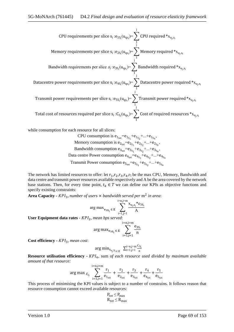
5G-MoNArch (761445) D4.2 Final design and evaluation of resource elasticity framework
Version 1.0 Page 69 of 153
CPU requirements per slice si :e1Si(uqsi)=∑CPU required
j
1
*xuj,si
Memory requirements per slice si :e2Si(uqsi)=∑Memory required
j
1
*xuj,si
Bandwidth requirements per slice si :e3Si(uqsi)=∑Bandwidth required
j
1
*xuj,si
Datacentre power requirements per slice si :e4Si(uqsi)=∑Datacentre power required
j
1
*xuj,si
Transmit power requirements per slice si :e5Si(uqsi)=∑Transmit power required
j
1
*xuj,si
Total cost of resources required per slice si :CSi(uqsi)=∑Cost of required resources
j
1
*xuj,si
while consumption for each resource for all slices:
CPU consumption is e1tot=e1S1+e1S2
+...+e1Sn ,
Memory consumption is e2tot=e2S1+e2S2
+...+e2Sn ,
Bandwidth consumption e3tot=e3S1+e3S2
+...+e3Sn ,
Data centre Power consumption e4tot=e4S1+e4S2
+...+e4Sn
Transmit Power consumption e5tot=e5S1+e5S2
+...+e5Sn
The network has limited resources to offer: let r1,r2,r3,r4,r5 be the max CPU, Memory, Bandwidth and
data centre and transmit power resources available respectively and A be the area covered by the network
base stations. Then, for every time point, 𝑡𝑘 ∈ 𝑇 we can define our KPIs as objective functions and
specify existing constraints:
Area Capacity - 𝐾𝑃𝐼1, number of users × bandwidth served per m2 in area:
arg maxe3Si ∈ E
∑xuj,si
*e3Si
A
i=n,j=m
i=1,j=1
User Equipment data rates - 𝐾𝑃𝐼2, mean bps served:
arg maxe3Si ∈ E ∑
e3Sin
i=n,j=m
i=1,j=1
Cost efficiency - 𝐾𝑃𝐼3, mean cost:
arg minxuj,Si ∈ E ∑
CSi
n
i=n,j=m
i=1,j=1
Resource utilisation efficiency - 𝐾𝑃𝐼4, sum of each resource used divided by maximum available
amount of that resource:
arg max Esi ∑
r1e1tot
+ r2e2tot
+r3e3tot
+r4e4tot
+r5e5tot
i=n,j=m
i=1,j=1
This process of minimising the KPI values is subject to a number of constrains. It follows reason that
resource consumption cannot exceed available resources:
Ptot ≤ Pmax Rtot ≤ Rmax
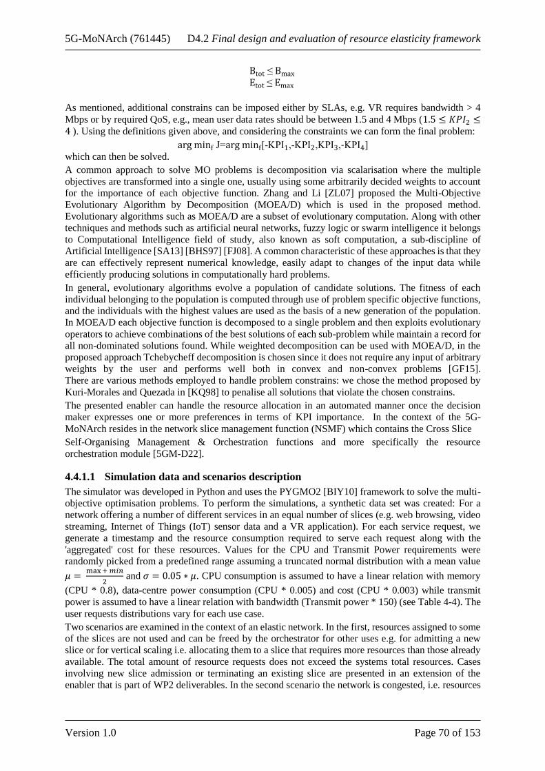
5G-MoNArch (761445) D4.2 Final design and evaluation of resource elasticity framework
Version 1.0 Page 70 of 153
Btot ≤ Bmax Etot ≤ Emax
As mentioned, additional constrains can be imposed either by SLAs, e.g. VR requires bandwidth > 4
Mbps or by required QoS, e.g., mean user data rates should be between 1.5 and 4 Mbps (1.5 ≤ 𝐾𝑃𝐼2 ≤4 ). Using the definitions given above, and considering the constraints we can form the final problem:
arg minf J=arg minf[-KPI1,-KPI2,KPI3,-KPI4] which can then be solved.
A common approach to solve MO problems is decomposition via scalarisation where the multiple
objectives are transformed into a single one, usually using some arbitrarily decided weights to account
for the importance of each objective function. Zhang and Li [ZL07] proposed the Multi-Objective
Evolutionary Algorithm by Decomposition (MOEA/D) which is used in the proposed method.
Evolutionary algorithms such as MOEA/D are a subset of evolutionary computation. Along with other
techniques and methods such as artificial neural networks, fuzzy logic or swarm intelligence it belongs
to Computational Intelligence field of study, also known as soft computation, a sub-discipline of
Artificial Intelligence [SA13] [BHS97] [FJ08]. A common characteristic of these approaches is that they
are can effectively represent numerical knowledge, easily adapt to changes of the input data while
efficiently producing solutions in computationally hard problems.
In general, evolutionary algorithms evolve a population of candidate solutions. The fitness of each
individual belonging to the population is computed through use of problem specific objective functions,
and the individuals with the highest values are used as the basis of a new generation of the population.
In MOEA/D each objective function is decomposed to a single problem and then exploits evolutionary
operators to achieve combinations of the best solutions of each sub-problem while maintain a record for
all non-dominated solutions found. While weighted decomposition can be used with MOEA/D, in the
proposed approach Tchebycheff decomposition is chosen since it does not require any input of arbitrary
weights by the user and performs well both in convex and non-convex problems [GF15].
There are various methods employed to handle problem constrains: we chose the method proposed by
Kuri-Morales and Quezada in [KQ98] to penalise all solutions that violate the chosen constrains.
The presented enabler can handle the resource allocation in an automated manner once the decision
maker expresses one or more preferences in terms of KPI importance. In the context of the 5G-
MoNArch resides in the network slice management function (NSMF) which contains the Cross Slice
Self-Organising Management & Orchestration functions and more specifically the resource
orchestration module [5GM-D22].
4.4.1.1 Simulation data and scenarios description
The simulator was developed in Python and uses the PYGMO2 [BIY10] framework to solve the multi-
objective optimisation problems. To perform the simulations, a synthetic data set was created: For a
network offering a number of different services in an equal number of slices (e.g. web browsing, video
streaming, Internet of Things (IoT) sensor data and a VR application). For each service request, we
generate a timestamp and the resource consumption required to serve each request along with the
'aggregated' cost for these resources. Values for the CPU and Transmit Power requirements were
randomly picked from a predefined range assuming a truncated normal distribution with a mean value
𝜇 = max+ 𝑚𝑖𝑛
2 and 𝜎 = 0.05 ∗ 𝜇. CPU consumption is assumed to have a linear relation with memory
(CPU * 0.8), data-centre power consumption (CPU * 0.005) and cost (CPU * 0.003) while transmit
power is assumed to have a linear relation with bandwidth (Transmit power * 150) (see Table 4-4). The
user requests distributions vary for each use case.
Two scenarios are examined in the context of an elastic network. In the first, resources assigned to some
of the slices are not used and can be freed by the orchestrator for other uses e.g. for admitting a new
slice or for vertical scaling i.e. allocating them to a slice that requires more resources than those already
available. The total amount of resource requests does not exceed the systems total resources. Cases
involving new slice admission or terminating an existing slice are presented in an extension of the
enabler that is part of WP2 deliverables. In the second scenario the network is congested, i.e. resources
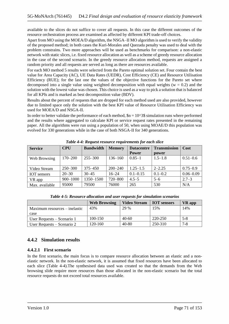
5G-MoNArch (761445) D4.2 Final design and evaluation of resource elasticity framework
Version 1.0 Page 71 of 153
available to the slices do not suffice to cover all requests. In this case the different outcomes of the
resource orchestration process are examined as affected by different KPI trade-off choices.
Apart from MO using the MOEA/D algorithm, the NSGA–II MO algorithm is used to verify the validity
of the proposed method; in both cases the Kuri-Morales and Quezada penalty was used to deal with the
problem constrains. Two more approaches will be used as benchmarks for comparison: a non-elastic
network with static slices, i.e. fixed resource allocation as well as a scheme of greedy resource allocation
in the case of the second scenario. In the greedy resource allocation method, requests are assigned a
random priority and all requests are served as long as there are resources available.
For each MO method 5 results were selected from the Pareto optimal solution set. Four contain the best
value for Area Capacity (AC), UE Data Rates (UEDR), Cost Efficiency (CE) and Resource Utilisation
Efficiency (RUE); for the last one the values of the objective functions for the Pareto set where
decomposed into a single value using weighted decomposition with equal weights (w = 0.2) and the
solution with the lowest value was chosen. This choice is used as a way to pick a solution that is balanced
for all KPIs and is marked as best decomposition value (BDV).
Results about the percent of requests that are dropped for each method used are also provided, however
due to limited space only the solution with the best KPI value of Resource Utilisation Efficiency was
used for MOEA/D and NSGA-II.
In order to better validate the performance of each method, $n = 10^3$ simulation runs where performed
and the results where aggregated to calculate KPI or service request rates presented in the remaining
paper. All the algorithms were run using a population of 50, when using MOAE/D this population was
evolved for 330 generations while in the case of both NSGA-II for 340 generations.
Table 4-4: Request resource requirements for each slice
Service CPU Bandwidth Memory Datacentre
Power
Transmission
power
Cost
Web Browsing 170–200 255–300 136–160 0.85–1 1.5–1.8 0.51–0.6
Video Stream 250–300 375–450 200–240 1.25–1.5 2–2.25 0.75–0.9
IOT sensors 20–30 30–45 16–24 0.1–0.15 0.1–0.2 0.06–0.09
VR app 900–1000 1350–1500 720–800 4.5–5 5–6 2.7–3
Max. available 95000 79500 76000 265 530 N/A
Table 4-5: Resource allocation and user requests for simulation scenarios
Web Browsing Video Stream IOT sensors VR app
Maximum resources – inelastic
case
43% 29 % 15% 14%
User Requests – Scenario 1 100-150 40-60 220-250 5-8
User Requests – Scenario 2 120-160 40-80 250-310 7-8
4.4.2 Simulation results
4.4.2.1 First scenario
In the first scenario, the main focus is to compare resource allocation between an elastic and a non-
elastic network. In the non-elastic network, it is assumed that fixed resources have been allocated to
each slice (Table 4-4).The synthesised data used was created so that the demands from the Web
browsing slide require more resources than those allocated in the non-elastic scenario but the total
resource requests do not exceed total resources available.

5G-MoNArch (761445) D4.2 Final design and evaluation of resource elasticity framework
Version 1.0 Page 72 of 153
Table 4-6: Aggregated mean KPI values for different solution choices – Scenario 1
KPI
Solution
Area
Capacity
UE data
Rate
Resource Ut.
Efficiency Cost Efficiency
MOEA/D (CE,AC,RUE)* 231.082 139.567 3.824 0.584
MOEA/D (UEDR) 224.783 175.352 3.440 0.592
MOEA/D (BDV) 231.163 142.826 3.785 0.588
NSGA-II (AC) 230.548 139.489 3.818 0.585
NSGA-II (UEDR) 196.942 157.551 3.041 0.597
NSGA-II (RUE) 230.539 139.487 3.819 0.585
NGSA-II (CE) 230.527 139.468 3.818 0.584
NSGA-II (BDV) 202.075 142.373 3.3441 0.585
Unelastic 217.179 215.591 2.789 0.605
* MOEA/D solutions for best AC, CE, RUE KPI values coincide in scenario 1
After the optimisation using MOEA/D for AC, REU or CE KPIs, the network resources are efficiently
allocated so no requests are rejected. In contrast, the legacy network cannot serve all requests, since
slices need more than allocated resources. Dashed red lines shows resource limits and red areas show
service degradation or rejection cases (see Figure 4-22).
In terms of KPI performance, different choices of MOEA/D outperform all the other optimisation
methods in terms of Area Capacity and Resource Utilisation and shares the best results in the Cost
Efficiency KPI with NSGA-II method. Concerning the ’balanced’ solution, MOEA/D - BDV solution
outperforms the corresponding NSGA-II solution in all KPIs apart from Cost Efficiency (Table 4-6).
Figure 4-22: Behaviour of instances of a (1) non-elastic and (2) elastic network optimised for
resource efficiency using MOEA/D, in Scenario 1
The suggested optimisation method clearly outperforms the NSGA-II approach in terms of requests that
either are dropped or will be served in a degraded state, since it is the only allocation method where all
requests are fully served (Table 4-7).
Table 4-7: Percent (%) of Requests that are dropped in Scenario 1
Method
Service
MOEA/D
(RUE)
NSGA-II (RUE) Inelastic
Web Browsing 0 0.002 3.353

5G-MoNArch (761445) D4.2 Final design and evaluation of resource elasticity framework
Version 1.0 Page 73 of 153
Video Stream 0 0.012 0
IoT Sensors 0 0.093 0
VR application 0 1.384 0
Average 0 0.373 0.838
4.4.2.2 Second scenario
In the second scenario, the available resource pool does not suffice to cover the service requests in at
least half (50%) of the cases examined in each simulation run. MOAE/D displays the best performance
(Table 4-8) in all KPIs apart from the Cost efficiency KPI, where the results using NGSA-II are better.
In all the cases apart from the UE data rate KPI, multi-objective methods produce better results
compared to an inelastic network.
Similar to the first scenario, the MOEA/D - BDV ’balanced’ solution, outperforms the corresponding
NSGA-II solution for all KPIs apart Cost Efficiency and the Greedy solution for all KPIs. Concerning
request drops when optimising for the Resource Utilisation KPI, using MOEA/D results in 4.087 %
drop, lower than the results of the inelastic approach but higher than the results of Greedy resource
allocation (Table 4-9). However, it should again be noted different service requests have different
resource utilisation needs thus contributing differently to the final value of Resource Utilisation.
Table 4-8: Aggregated mean KPI values for different solution choices – Scenario 2
KPI
Solution
Area Capacity UE Data Rate Resource Ut. Efficiency Cost Efficiency
MOEA/D (AC) 334.91 185.402 4.666 0.592
MOEA/D (UEDR) 316.627 210.038 4.271 0.604
MOEA/D (RUE) 334.854 185.622 4.762 0.592
MOEA/D (CE) 334.421 187.341 4.631 0.593
MOEA/D (BDV) 333.63 175.614 4.754 0.586
NSGA-II (AC) 334.347 179.54 4.713 0.589
NSGA-II (UEDR) 284.19 179.682 3.936 0.589
NSGA-II (RUE) 334.497 179.496 4.711 0.588
NSGA-II (CE) 334.347 178.682 4.711 0.589
NSGA-II (BDV) 294.507 157.98 4.3921 0.564
Greedy 292.804 151.895 4.588 0.589
Unelastic 295.145 205.47 3.646 0.617
Table 4-9: Percent (%) of Requests that are dropped in Scenario 2
Service
Method
MOEA/D
(RUE)
NSGA-II
(RUE)
Greedy Unelastic
Web Browsing 0.052 0.284 2.405 14.179
Video Stream 0.03 0.855 2.35 4.513
IoT Sensors 12.505 8.894 2.401 16.057
VR application 3.762 4.902 2.441 0
Average 4.087 3.734 4.045 8.687
4.4.3 KPI takeaways
We approached resource orchestration of a 5G network with slices as a multi-objective problem. A
scheme based on an evolutionary algorithm, MOEA/D, was proposed to optimise a number of network

5G-MoNArch (761445) D4.2 Final design and evaluation of resource elasticity framework
Version 1.0 Page 74 of 153
key performance indicators in a simultaneous manner, using these results to effectively allocate network
resources to the network slices. To facilitate an easier overview of the enabler gains, Table 4-10 presents
the percentage difference between the KPI values resulting by the orchestrating the network with the
proposed enabler compared to in an inelastic network and the greedy allocation scheme described in
4.4.1.
Table 4-10: Percentage difference of enabler results compared to unelastic and greedy network
schemes
Area Capacity
- MOEA/D
(AC)
UE data rate -
MOEA/D
(UEDR)
Resource utilisation
efficiency MOEA/D
(RUE)
Cost efficiency -
MOEA/D
(BDV)
Scenario 1 –
Unelastic network
6.238 % -20.585 % 31.30% -3.532 %
Scenario 2 –
Unelastic network
12.622 % 2.199 % 26.546 % -5.158 %
Scenario 2 – Greedy
allocation
13.416 % 32.139 % 3.722 % -0.51 %
4.5 Slice-aware elastic resource management
The aim of the slice-aware elastic resource management is to allocate the available physical resources
among different slices with different serving priority and QoS requirements. The developing approach
in this framework has two main parts: a) allocation of radio resources to each slice b) allocating enough
computational resource to each slice to process the assigned radio resources. As it is discussed in [5GM-
D41], the resource management in multi-tenant virtual environment has four main steps:
• Forming the available resource pool,
• Estimating the total radio and computational capacity,
• Allocation of available resources to different slices,
• Observation and update.
The developed slice-aware resource management in the scope of this project uses AI-based approaches
to improve the resource allocation elasticity and utilisation.
4.5.1 AI-based slice-aware resource management
The common Radio Resource Management (RRM) algorithms either can allocate resources in passive
mode (i.e. adopt the allocation after observation of demand change) or they allocate based on maximum
demand assumption. To improve the elasticity in resource allocation and increase the radio resource
utilisation, the algorithms need to have a prediction of demands to enable elastic resource allocation.
The demand prediction is even more important in computational resource orchestration and
management. Creating a new instance in the cloud environment can take up to several hundred
milliseconds. Provisioning of the VNF chains for the high-load leads to extra CAPEX and OPEX but
the prediction of traffic demands for network slices enables the elastic computational resource
management and Cost efficiency.
The proposal is to train a Deep Neural Network (DNN) with the historical data and records to predict
the traffic demand in the next design interval based. The prediction is based on traffic demand in N-
previous intervals. After observing the demand in each interval, the neural network fast retraining can
update. This way it can cope with slow and long-term changes in traffic pattern behaviour. It worth
noting that the predictor cannot predict the sudden variation of traffic and it predicts the average demand
in the next time interval. The traffic predictor in this paper, is a deep neural network with 2 dens layers
of 16 neurons and ReLU activation function and a sigmoid activation function for the output layer.
Figure 4-23.a presents the deep Neural network architecture with two dense layers with ReLU activation
function. It is used to predict the traffic demands of two network slices with different behaviour and
Figure 4-23.b shows the predicted against the actual traffic. Virtual resource management models,

5G-MoNArch (761445) D4.2 Final design and evaluation of resource elasticity framework
Version 1.0 Page 75 of 153
consequently, can now consider also predicted slice demands to adapt the service provisioning; for
example, some services may have a reparative pattern or may only be active during certain times of the
day or year.
Figure 4-23: Traffic demand prediction using deep learning
Having the prediction of demand, the allocation optimisation model can be modified to consider
allocating radio resource based on the demand of each network slice. The computational resources then
are allocated after determining how many PRBs are allocated to each network slice. Based on allocated
radio resources to each slice, the computational resource management algorithm takes the computational
models for each VNF and decides how many computational resources to allocate to each network slice.
The computational modelling for PHY layer is presented in the last section. In the same research path,
the profiling of the higher layers is presented in Section 5.5.
4.5.2 Slice-aware elastic resource management model
The allocation of available radio resources to different network slices can be formulated as the
optimisation problem to maximise the weighted network throughput subject to constraints including the
Service Level Agreements (SLAs), the total network throughput, and fairness in addition to under-
stacking and violation penalties. The propose model is based on the model described in [KCFC+17] but
it is modified to consider the traffic demand of each slice. The former models ignore the traffic demands
of the network slices, which it can be interpreted as assuming that the network slices always have higher
demands than the allocated radio resources; Hence, they can always fully utilise the radio resources
allocated to them. In the new model, the deep neural networks first predict the traffic demands and this
prediction can be corrected with a confidence coefficient
𝑅𝑏𝑖[Mbps]𝑃𝑟𝑒 = 𝛾𝑖𝑅𝑏𝑖[Mbps]
𝑃𝑟��
where:
• 𝑅𝑏𝑖𝑃𝑟𝑒: the corrected demand prediction for slice i,
• 𝑅𝑏𝑖𝑃𝑟𝑒 : the demand predicted by the DNN for slice i,
• 𝛾𝑖: the correction factor for slice i.

5G-MoNArch (761445) D4.2 Final design and evaluation of resource elasticity framework
Version 1.0 Page 76 of 153
In addition to traffic prediction, the inter-slice radio resource management model has two other essential
part: i) Estimation of the total network throughput, ii) Allocation available resource to the network slices.
Estimation of the Total Network Throughput
The models for inter-slice radio resource management model, in first step, map the number of available
Physical Radio Blocks (PRBs) to the total network throughput [KC14]. The achieved data rate by
assigning a single PRB to a terminal varies based on different parameter such as the channel quality and
the selected Modulation and Coding Scheme (MCS). Nevertheless, it is possible to have the data rate of
a PRB as a function of Signal-to-Interference-plus-Noise (SINR). Based on the distribution for SINR is
by modelling the network as a K-tier network, in which the Radio Remote Heads (RRHs) are spatially
distributed as a Poisson Point Process (PPP) with a given density and transmission power, the Probability
Density Function (PDF) of a single PRB can be calculated. The convolution of PDF of all the available
PRBs provides, the PDF of the total network throughput, assuming the channels are independent.
Finally, the estimation of the available network capacity is possible by having the PDF and CDF
(Cumulative Density Function) of the total networks data rate. This estimation is crucial in the allocation
of resources described in the next sections. Using the same approach, one can map the allocated
throughput, i.e. the output of the optimisation, to each network slice to the number of required PRBs.
Radio Resource Allocation to Slice
The proposed model for allocation of radio resources to different network slices is a multi-objective
optimisation model. These objectives while related, they may be contradictive. The objectives are as
follows:
Slice Priority is the primary objective in the proposed model and aims to allocate more radio resources
and higher throughput to the slices with higher priority. Hence, the related objective function in the
model is the weighted throughput given by:
𝑓𝑆𝑟𝑣(𝑹𝒃𝑺𝒓𝒗) =∑𝑤𝑖
𝑆𝑟𝑣𝑅𝑏𝑖[Mbps]𝑆𝑟𝑣
𝑁𝑠
𝑖=0
where:
• 𝑓𝑆𝑟𝑣: slice priority objective function,
• 𝑹𝒃𝑺𝒓𝒗: vector of serving throughputs,
• 𝑅𝑏𝑖𝑆𝑟𝑣: serving (allocated) throughput to slice i,
• 𝑁𝑠: number of network slices,
• 𝑤𝑖𝑆𝑟𝑣: serving weight of slice i.
The serving weights in the equation above defines the priority of slices. The slice with relatively higher
serving weight is have relatively higher priority and the model tend to allocate more resources to it
comparing to the other slices. It is common practice to have the summation of the serving weights equal
to unit.
Understocking is the focus of the second objective function. It is ideal to allocate to each slice what they
are going to demand. However, there are cases where there are not enough resources available to serve
all the requested throughput from all the network slices. In these situations, the allocated throughput to
each slice is going to be smaller than the predicted demand. The understocking, in the framework of this
paper, is a non-negative value equal to difference of the predicted demand of a slice and the serving
throughput of the same slice. The model tries to minimise the summation of understocking throughput
given by:
𝑓𝑢𝑠(𝑹𝒃𝒖𝒔) = ∑𝑅𝑏𝑖[Mbps]
𝑢𝑠
𝑁𝑠
𝑖=0
where:
• 𝑓𝑢𝑠: understocking objective function,
• 𝑹𝒃𝒖𝒔: vector of understocking throughputs,
• 𝑅𝑏𝑖𝑢𝑠: understocking throughput to slice i, given by:

5G-MoNArch (761445) D4.2 Final design and evaluation of resource elasticity framework
Version 1.0 Page 77 of 153
𝑅𝑏𝑖𝑢𝑠 = min {0, 𝑅𝑏𝑖[Mbps]
𝑃𝑟𝑒 − 𝑅𝑏𝑖[Mbps]𝑆𝑟𝑣 }
It is worth noting that the correction factor introduced in the equation above contains the overstocking
(i.e. allocation of resources to a network slice more than the predicted demand.
Violation of Service Level Agreements (SLAs) is the next objective in the inter-slice radio resource
management model. The allocated resources to each network slice should meet the requirements dictated
by the SLA of the slice. While slices may have different SLAs, as it is introduced in [5GM-D41], the
three main SLAs categories are as follows:
1. Guaranteed Bitrate (GB): This type of SLA guarantees the network slice throughput to be
higher than the minimum guaranteed data rate and less than maximum guaranteed data rate.
𝑅𝑏𝑖[Mbps]𝑚𝑖𝑛 ≤ 𝑅𝑏𝑖[Mbps]
𝑆𝑟𝑣 ≤ 𝑅𝑏𝑖[Mbps]𝑚𝑎𝑥
where:
𝑅𝑏𝑖𝑚𝑖𝑛: minimum guaranteed data rate for slice i,
𝑅𝑏𝑖𝑚𝑎𝑥: maximum guaranteed data rate for slice i,
2. Best effort with minimum Guaranteed (BG): The minimum throughput for the network slice
is guaranteed in this type of SLA. However, allocation of more resource is subject to availability
of resources.
𝑅𝑏𝑖[Mbps]𝑚𝑖𝑛 ≤ 𝑅𝑏𝑖[Mbps]
𝑆𝑟𝑣
3. Best Effort (BE): A network slice with best effort SLA is only served when there are resources
available and no throughput is guaranteed.
So, the model should not allow any violation of SLAs. Under circumstances where the violation of SLAs
is unavoidable (e.g. when there are not enough resources) then the summation of violations has to be
minimised. The SLAs violations, 𝑅𝑏𝑣, is the difference between the demanded guaranteed data rate, given
by:
𝑅𝑏𝑖[𝑀𝑏𝑝𝑠]𝑣 = min {𝑅𝑏𝑖[Mbps]
𝑃𝑟𝑒 , 𝑅𝑏𝑖[Mbps]𝑚𝑖𝑛 } − 𝑅𝑏𝑖[Mbps]
𝑆𝑟𝑣
Fairness is the final objective the new model for inter-slice radio resource management. Although it is
desirable to serve the slice with relatively higher serving weights (i.e. high priority slices) with higher
throughput, not serving the other slices is not an acceptable output. The last objectives in the model
ensure that the slices receive the predicted demand data rate when there are enough resources. However,
the fairness objective in this model makes sure the violation of SLAs and understocking are distributed
among all the slices based on their priority in the congestion situations.
In the case of understocking, demands and serving weight are the two parameters, which the fairness
considers. Regarding demands, it is only fair if the understocking of slices with high demands to be
higher. For example, 10 Mbps understocking for a slice with 100 Mbps demand as well as a slice with
10 Mbps is not fair. In the former case the slice received 90% of what it has demands while in the latter
case the slice is not served all. Now assume that both slices have the same amount of demand, but their
serving weights are different. The fair allocation suggests the slice with higher serving weight (i.e. the
more important slice) experience less understocking.
Hence, a fair resource allocation considering understocking is when the condition below is achieved:
∀𝑖: |𝑤𝑖𝑆𝑟𝑣𝑅𝑏𝑖[𝑀𝑏𝑝𝑠]
𝑢𝑠
𝑅𝑏𝑖[𝑀𝑏𝑝𝑠]𝑝𝑟𝑒 −
1
𝑁∑
𝑤𝑗𝑆𝑟𝑣𝑅𝑏𝑗[𝑀𝑏𝑝𝑠]
𝑢𝑠
𝑅𝑏𝑗[𝑀𝑏𝑝𝑠]𝑝𝑟𝑒
𝑁𝑠
𝑗=0
| = 0
In the case of violations, the fairness only considers the violation weights, 𝑤𝑖𝑣 . Thus, the fairness
condition in this situation is:
∀𝑖: |𝑤𝑖𝑣𝑅𝑏𝑖[𝑀𝑏𝑝𝑠]
𝑣 −1
𝑁∑𝑤𝑗
𝑣𝑅𝑏𝑗[𝑀𝑏𝑝𝑠]𝑣
𝑁𝑠
𝑗=0
| = 0
However, it is always neither possible (i.e. the constraint imposed by SLA) nor desirable to satisfy the
above conditions, but the goal is to minimise the diversion from these conditions. Hence, the objective
function for fairness is:

5G-MoNArch (761445) D4.2 Final design and evaluation of resource elasticity framework
Version 1.0 Page 78 of 153
𝑓𝑓 (𝑹𝒃𝒇𝒖𝒔 , 𝑹𝒃
𝒇𝒗) = ∑ 𝑅𝑏𝑗[𝑀𝑏𝑝𝑠]𝑓𝑣 + 𝑅𝑏𝑗[𝑀𝑏𝑝𝑠]
𝑓𝑢𝑠
𝑁𝑠
𝑗=0
here:
• 𝑓𝑓: fairness objective function,
• 𝑹𝒃𝒇𝒖𝒔: vector of understocking fairness derivation,
• 𝑅𝑏𝑖𝑓𝑢𝑠: understocking fairness derivation for slice i,
• 𝑹𝒃𝒇𝒗: vector of violation fairness derivation,
• 𝑅𝑏𝑖𝑓𝑣: violation fairness derivation for slice i,
Based on the objectives discussed above, a multi-objective linear program optimisation problem as
follows:
𝑚𝑎𝑥𝑅𝑏
𝑓𝑆𝑟𝑣(𝑹𝒃𝑺𝒓𝒗) − 𝛼𝑓𝑓
𝑓(𝑅𝑏𝑓𝑣 , 𝑅𝑏
𝑓𝑢𝑠) + 𝛼𝑣𝑓𝑣(𝑅𝑏
𝑣) + 𝛼𝑢𝑠𝑓𝑢𝑠(𝑅𝑏
𝑢𝑠)
𝑠. 𝑡.
{
∑𝑅𝑏𝑖[𝑀𝑏𝑝𝑠]𝑆𝑟𝑣 ≤ 𝑅𝑏[𝑀𝑏𝑝𝑠]
𝑡𝑜𝑡
𝑁𝑠
𝑖=0
|𝑤𝑖𝑆𝑟𝑣𝑅𝑏𝑖[𝑀𝑏𝑝𝑠]
𝑢𝑠
𝑅𝑏𝑖[𝑀𝑏𝑝𝑠]𝑝𝑟𝑒 −
1
𝑁∑
𝑤𝑗𝑆𝑟𝑣𝑅𝑏𝑗[𝑀𝑏𝑝𝑠]
𝑢𝑠
𝑅𝑏𝑗[𝑀𝑏𝑝𝑠]𝑝𝑟𝑒
𝑁𝑠
𝑗=0
| ≤ 𝑅𝑏𝑖[𝑀𝑏𝑝𝑠]𝑓𝑠𝑟𝑣
|𝑤𝑖𝑣𝑅𝑏𝑖[𝑀𝑏𝑝𝑠]
𝑣 −1
𝑁∑𝑤𝑗
𝑣𝑅𝑏𝑗[𝑀𝑏𝑝𝑠]𝑣
𝑁𝑠
𝑗=0
| ≤ 𝑅𝑏𝑖[𝑀𝑏𝑝𝑠]𝑓𝑣
𝑚𝑖𝑛 {𝑅𝑏𝑖[𝑀𝑏𝑝𝑠]𝑃𝑟𝑒 , 𝑅𝑏𝑖[𝑀𝑏𝑝𝑠]
𝑚𝑖𝑛 } − 𝑅𝑏𝑖[𝑀𝑏𝑝𝑠]𝑆𝑟𝑣 ≤ 𝑅𝑏𝑖[𝑀𝑏𝑝𝑠]
𝑣
𝑅𝑏𝑖[Mbps]𝑆𝑟𝑣 ≤ 𝑅𝑏𝑖[Mbps]
𝑚𝑎𝑥
where:
• 𝑅𝑏𝑡𝑜𝑡: the total network throughput,
• 𝛼𝑓: weight of fairness objective,
• 𝛼𝑣: weight of volition objective,
• 𝛼𝑢𝑠: weight of understocking objective.
It worth noting that the desired values for the fairness, violation, and understocking objective function
is zero while as the total network throughput increases, the weighted sum of the slice data rate, i.e. the
main objective function, increases. Hence, the weights of the other objective functions should be relative
to the total network throughput. However, these studies consider a comparative big weight (>10000
times of the total network’s throughput) as the objective weights.
4.5.3 Computational resource provisioning
Profiling the computational complexity of the network function is essential for provisioning and
allocation of computational resources in the virtual multi-tenant environment. The virtualisation of
networks is going to change the business models and the stakeholder models. One of these changes is
the emergence of small to medium size Small and Medium Enterprises (SMEs) as VNF providers, which
are going to offer different set of VNFs as their product. Different realisation of a VNF may have
different computational performance while the functionality of the VNF stay the same, e.g. a PCDP
module from two different providers. Hence, the modelling of computational complexity of VNFs has
to be updated not only for different VNFs but also for the same VNFs provided from different VNF
providers.
The work in [KSR18] presented the computational modelling of PHY layer of RAN based on Open Air
Interface (OAI) realisation [OAI]. After measuring the processing time of different network functions,
the correct coefficients are chosen using the Lasso technique [Tib96] to map the processing time to the

5G-MoNArch (761445) D4.2 Final design and evaluation of resource elasticity framework
Version 1.0 Page 79 of 153
relevant input variables (e.g. Modulation and Coding Scheme, MCS), CPU frequency, and number of
processing PRBs)., as follows:
𝜏𝑝[𝜇𝑠] =𝑁𝑃𝑅𝐵
𝑓[GHz ]2 ∑𝛼𝑖
′(𝐼𝑚𝑐𝑠)𝑖
2
𝑖=𝑜
where:
• 𝜏𝑝: the measured processing time,
• 𝑁𝑃𝑅𝐵: number of PRBs processed by the network function,
• 𝑓2: working frequency of the CPU of host machine,
• 𝛼𝑖′: model’s coefficients presented in [KSR18],
• 𝐼𝑚𝑐𝑠: the index of selected MCS.
Having the model for the computational complexity, the Infrastructure Provider (InP) can provision the
required computational resources (i.e. CPU cores) to process the traffic. Elastic management of
computational resources enables InP to offer the acceptable QoS while reducing its costs. Hence, proper
provisioning of the resources is essential step toward implementation of elastic resource management in
a multi-slice environment.
Based on the computational models for the VNFs, the required computational resources can be
calculated based on the probability function for input SINR and its mapping to MCS index. The
Cumulative Density Function (CDF) of SINR in a generic scenario can be modelled as [DGB+12]:
𝐶𝐷𝐹𝜌(𝜌[𝑑𝐵]) = 1 − 𝑒−0.46𝛼𝑝
𝜌[𝑑𝐵]
where:
• 𝜌: the SINR,
• 𝛼𝑝: pathloss exponent, 𝛼𝑝 ≥ 2.
The mapping of SINR to MCS index is highly dependent on the implemented link adaptation techniques,
which with acceptable simplifications can be model as a linear function as follows:
𝜌[𝑑𝐵] = 𝛾1𝐼𝑀𝐶𝑆 + 𝛾0
Hence, the CDF of processing time of a PRB is:
𝐶𝐷𝐹𝜏𝑝(𝜏𝑝[us]|𝜏𝑝[us]𝑚𝑖𝑛 ≤ 𝜏𝑝[us] ≤ 𝜏𝑝[us]
𝑚𝑎𝑥) = 𝑒
−0.46𝛼𝑝
(𝛾0+𝛾1∆(𝜏𝑝[us]
𝑚𝑖𝑛 )
2𝛼2′ )
− 𝑒−0.46𝛼𝑝
(𝛾0+𝛾1∆(𝜏𝑝[us])
2𝛼2′ )
𝑒
−0.46𝛼𝑝
(𝛾0+𝛾1∆(𝜏𝑝[us]
𝑚𝑖𝑛 )
2𝛼2′ )
− 𝑒
−0.46𝛼𝑝
(𝛾0+𝛾1∆(𝜏𝑝[us]
𝑚𝑎𝑥)
2𝛼2′ )
where:
∆(𝜏𝑝[us]) = √𝛼1′ 2 + 4𝛼2
′ (𝑓[GHz ]2 𝜏𝑝[us] − 𝛼0
′ )
The Probability Distribution Function (PDF) of the processing time a VNF, when it is processing 𝑁𝑃𝑅𝐵,
is 𝑁𝑃𝑅𝐵 time auto-convolution of the PDF. The final output can be used to decide how many PRBs each
CPU core is supposed to process.
The Probability Density Function (PDF) of the processing time a VNF, when it is processing 𝑁𝑃𝑅𝐵, is
𝑁𝑃𝑅𝐵 time auto-convolution of the PDF. The final output can be used to decide how many PRBs each
CPU core is supposed to process.
4.5.4 Numerical results
The chosen scenario to evaluate the performance of the inter-slice radio resource management model is
based on the scenarios described in [KC14]. The scenario considers a serving area, which contains
16 cells with radius of 400 m each with 500 PRBs. The total network throughput estimated is 1.2 Gbps.
The terminals in this scenario require the average throughput of 13 Mbps for each terminal [Cisc18] and
the network slices contract data rates relative to their number of terminals.

5G-MoNArch (761445) D4.2 Final design and evaluation of resource elasticity framework
Version 1.0 Page 80 of 153
𝑅𝑏[Mbps]𝐶𝑜𝑛𝑡 = 𝑁𝑢𝑒𝑅𝑏[Mbps]
𝑢𝑒
where:
• 𝑅𝑏𝐶𝑜𝑛𝑡: the contracted data rate of slice,
• 𝑁𝑢𝑒: the number of User Equipment (UE),
• 𝑅𝑏𝑢𝑒: the average data rate per UE.
In addition, there are three network slices with three different SLAs. Slice GB has guaranteed data rate
SLA and the allocation of resources has to guaranteed throughput between 50% up to 100% of its
contracted data rates. While the BE slice has only minimum guaranteed data rate of 25% of its contracted
data rate. Finally, the allocation of resources to slice BE is subject to availability or resources. All three
slices have the same services and the same contracting data rate. Table 4-11 summarises the serving,
understocking, and violation weight for different slices.
Table 4-11: Weights and the SLAs for the slices
𝒘𝒊𝑺𝒓𝒗 𝒘𝒊
𝒗 𝑹𝒃𝒊[Mbps]
𝒎𝒊𝒏 𝑹𝒃𝒊[Mbps]
𝒎𝒂𝒙
GB 0.07 0.63 0.5𝑅𝑏𝐶𝑜𝑛𝑡 𝑅𝑏
𝐶𝑜𝑛𝑡
BG 0.02 0.18 0.25𝑅𝑏𝐶𝑜𝑛𝑡 N/A
BE 0.01 0.09 0 N/A
In the first step, the performance of the inter-slice radio resource management proposed in this paper is
evaluated under the full-demand mode (i.e. when the network slices demand all the contracted data
rates). In this case study, the number of UEs per slice is swept from 10 active terminal up to 350
terminals. Figure 4-24 illustrates the allocated throughput to each network slices as the function of
number of UEs per slice.
Figure 4-24: The allocated throughput to each network slice in full-demand
According to the figure, the total traffic demands per slice increases up 1.5 Gbps. Given the 1.2 Gbps
network capacity, it is not possible to serve all the slices when all off have the full demanded throughput.
The graph shows that the understocking (i.e. not serving the demanded throughput) starts happening
when the demand per slice reaches to 0.38 Gbps. As the demands per slice increases, slice GB with the
highest serving weights comparatively receives higher throughput than the slice BE with lowest serving
weights. The slice BE does not receive any more resources. The violation to the minimum guaranteed
data rate of slice BG happens when the total number of UEs reach to 80 terminals and they demand the
total throughput of 1.05 Gbps.

5G-MoNArch (761445) D4.2 Final design and evaluation of resource elasticity framework
Version 1.0 Page 81 of 153
In the next step, the number of UEs per slice is fixed to 180 but they are not demanding all the contracted
traffic. The traffic of slice BG is fixed on 45% of contracted data rates equal to 2.05 Gbps while the
demand of the slice GB is increasing the demand of slice BE is decreasing. Figure 4- presents the
predicted demand versus the allocated throughput in 20 observation intervals.
Figure 4-: Resource allocation to the slices with demand prediction
It is apparent that the slice BE and BG are also received the full demanded throughput up to ninth
observation interval, where the demand of the slice GB passed 336.4 Mbps. Comparing the numeric
results from Figure 4-24 and Figure 4- demonstrates the multiplexing gain using the throughput
prediction. Using the former algorithms, the slice BE would have not received any throughput. The slice
BG also is experiencing higher data rates since the most important slice, the slice GB, is not fully
requesting its contracted data rates.
It can be concluded that the second scenario, the new model increases the elasticity of resource
allocations. The target KPIs effected with this algorithm is the total served throughput and the required
number of CPUs. While the maximum total network throughput has not changed, the results show that
the total served throughput can increases. The algorithm can improve the complexing gain by sharing
the infrastructure among multiple slices. Also, the proposed algorithm can now scale the computational
resources according to traffic demands and allocated radio resources. Hence, the required computational
resources (i.e. total active CPUs time) reduces. These changes of to KPIs above can finally translate to
more cost-efficient realisation of network. It also can be represented as better service quality offer with
the same amount of CAPEX.

5G-MoNArch (761445) D4.2 Final design and evaluation of resource elasticity framework
Version 1.0 Page 82 of 153
5 Elastic resource management
With the mushrooming of different services provided by different tenant of the network envisioned by
5G, the slow scale, rather static and immutable resource allocation strategies that were usually adopted
by previous generation will be soon outdated. That is, elastic orchestration algorithms are needed to
efficiently exploit multiplexing gains across slices. While the algorithms presented in Chapter 4, we also
focused on the resource assignment problem from an artificial intelligence perspective, in this Chapter
we first provide a proof of the importance of elastic orchestration algorithms (Section 5.1) and then
specify a number of them along with their numerical results.
Figure 5-1: Innovations on elastic resource management on top of 5G-MoNArch architecture
The enablers described in this Chapter are mostly related to the efficient orchestration, so they mostly
reside in the MANO layer, either encompassing all the elements (Slice-aware computational resource
allocation in Section 5.3 or Game Theory Approach to Resource Assignment in Section 5.4) or a specific
one (the VIM, for the Profiling of computational complexity of RAN, Section 5.5). Finally, we also
define a specific Network Function that is able to translate such resource assignment into practice (the
Slice Aware Automatic RAN Configuration, Section 5.2).
5.1 Data driven multi-slicing efficiency
Network slicing has profound implications on resource management. When instantiating a slice, an
operator needs to allocate sufficient computational and communication resources to its VNFs. In some
cases, these resources may be dedicated, becoming inaccessible to other slices [SPF+17]. Alternatively,
elastic orchestration algorithms can be employed to dynamically allocate resources to slices based on
the time-varying demands of tenants [FMK17, KN17] following the elastic orchestration framework
described above. Such algorithms introduce additional complexity, and may in some cases hinder
resource isolation, the corresponding guarantees to tenants, and/or the ability to deploy fully customised
slices.
Slice-aware computational resource allocation
Slice-aware Automatic RAN Configuration
Game theory approach to Resource Assignment
Profiling of computational complexity of RAN

5G-MoNArch (761445) D4.2 Final design and evaluation of resource elasticity framework
Version 1.0 Page 83 of 153
Figure 5-2: Network slicing types from a resource utilisation perspective
Figure 5-2 shows that there is an inherent trade-off among: i) service customisation, which favours the
deployment of specialised slices with tailored functions for each service and, possibly, dedicated and
guaranteed resources; ii) resource management efficiency, which increases by dynamically sharing the
resources of the common infrastructure among the different services and slices; and, (iii) system
complexity, resulting from deploying more dynamic resource allocation mechanisms that provide higher
efficiency at the cost of employing elaborate operation and maintenance functions [SCS16].
Slicing strategies can be categorised as in Figure 5-2. In general, slicing strategies at the higher network
layers provide a lower level of customisation yet they can more easily achieve efficient resource sharing
without additional complexity. Indeed, when slicing occurs at high layers (e.g., type-A), the operator
cannot offer full customisation, but it can easily employ highly dynamic allocation schemes for the lower
layers; in contrast, achieving such an efficient resource allocation is much more challenging when
considering network slicing schemes with stringent customisation requirements (i.e., strategies
involving the lower layers down to type-E slicing). For instance, when all slices have a common MAC
layer, an efficient sharing of radio resources is easy, yet MAC is not tailored to their different needs;
conversely, if each slice implements a different, customised MAC protocol, it is more difficult to
efficiently share radio resources.
So, our aim here is to shed light on the trade-offs between customisation, efficiency, and complexity in
network slicing, by evaluating the impact of resource allocation dynamics at different network points.
Based on our analysis, it is thus possible to determine in which cases the gains in efficiency are worth
the sacrifice in customisation/isolation and/or the extra complexity. Since resource management
efficiency in network slicing highly depends on the traffic patterns of different services supported by
the various slices, we build on substantial service-level measurement data collected by a major operator
in a production mobile network, and:
• quantify the price paid in efficiency when suitable algorithms for dynamic resource allocation
are not available, and the operator has to resort to physical network duplication;
• evaluate the impact of sharing resources at different locations of the network, including the
cloudified core, the virtualised radio access, or the individual antennas;
• outline the benefit of dynamic resource allocation at different timescales, i.e., allowing to
reallocate resources across slices with different reconfiguration intervals.
5.1.1 Networks scenario and metrics
5.1.1.1 Networks slicing scenario
Let us consider a mobile network providing coverage to a generic geographical region, where mobile
subscribers consume a variety of heterogeneous services. The operator owning the infrastructure
implements slices s ∈ S, each dedicated to a different subset of services.
Dedicated Resources
Q
I
0000 0100 1100 1000
0001 0101 1101 1001
0011 0111 1111 1011
0010 0110 1110 1010
Antenna Spectrum RAN
processing
Radio Resource
Management
Edge
Cloud
Core
Cloud
Type A Slice
Type B Slice
Type C Slice
Type D Slice
Type E Slice
Shared Resources

5G-MoNArch (761445) D4.2 Final design and evaluation of resource elasticity framework
Version 1.0 Page 84 of 153
Figure 5-3: Hierarchical mobile network architecture
We assume that each slice can be implemented according to any of the strategies in Figure 5-2. To
capture such a general scenario, we model the mobile network architecture as a hierarchy composed by
a fixed number of levels (𝑙 = 1, … , L) ordered from the most distributed (l = 1) to the most centralised
(l = L), as illustrated in Figure 5-3. Every network level l is composed by a set 𝐶𝑙 of network nodes,
each serving a given number of base stations. In the two extremes, we have 𝑙 = 1, where network nodes
in 𝐶1 have a bijective mapping to individual antennas, and 𝑙 = L, where 𝐶𝑙 contains a single network
node controlling all antennas in the whole target region. In between, for 1 < 𝑙 < L, the number of network
nodes in 𝐶𝑙 decreases with 𝑙 , whereas that of base stations served by each such node increases
accordingly. This allows us to capture a wide range of network slicing deployment from the edge (lower
values for 𝑙) to the centre cloud (higher ones).
5.1.1.2 Slice specification
Network slicing allows the operator to fulfil minimum QoS requirements requested by each tenant. We
capture such requirements as a slice specification z, which is established so as to ensure a sufficient
service quality for the slice demands. More precisely, a slice specification involves:
(i) Guaranteed time fraction f : the operator engages to guarantee that the traffic demand of the slice is
fully serviced during at least a fraction f ∈ [0, 1] of time.
(ii) Averaging window length w: the operator commitment on fraction f above is intended on discrete-
time demands of granularity w, with traffic averaged over the disjoint time windows of duration w.
To ensure compliance with the requirements, the operator shall guarantee that enough resources are
allocated to all slices s ∈ S at every node c ∈ 𝐶𝑙 of each network level 𝑙. Formally, the required amount
of resources needed to meet a slice specification z = (f ,w) is computed as follows.
Let 𝑜𝑐,𝑠(𝑡) denote the load offered by slice s at node c and time t; also, let 𝑜𝑐,𝑠(𝑘) (k) = 1
𝑤∫ 𝑜𝑐,𝑠(𝑡) 𝑑𝑡𝑡
𝑘
be the average load over window k covering a time interval of the s me name with duration w. Let us
also denote by 𝑟𝑐,𝑠𝑧 (𝑘) the amount of resources allocated to slice s at node c during window k. According
to the above requirements, 𝑟𝑐,𝑠𝑧 (𝑘) has to be set such that the following inequality holds
P (rc,sz (k) ≥ oc,s(k)) ≥ f,
where P (·) denotes the probability of the argument. Basically, the above equation states that the
resources allocated should meet the demand for at least a fraction f of averaging windows
5.1.1.3 Resource allocation to slices
In presence of elastic orchestration algorithms, the resource allocation can be re-modulated over time.
If, at some node c, one could reallocate resources at every averaging window, it would be sufficient to
assign to a slice s the resources it requires during that window with probability at least f, according to
the above equation. However, in practice the periodicity of reconfiguration is limited by the adopted
slicing strategy (see Figure 5-2.) as well as by the constraints of the underlying technology.

5G-MoNArch (761445) D4.2 Final design and evaluation of resource elasticity framework
Version 1.0 Page 85 of 153
Let us assume that τ ≫ w is the minimum time needed for resource reallocation, which we refer to as a
reconfiguration period. Let us denote by n ∈ T the 𝑛𝑡ℎreconfiguration period within the set T of all the
reconfiguration periods that compose the whole system observation time; also, rc,sz (n)
is the amount of resources allocated to slice s in node c during the reconfiguration period n, under
specification z. Since no reassignment is possible within a reconfiguration period, then 𝑟𝑐,𝑠𝑧 (𝑘)= 𝑟𝑐,𝑠
�� (𝑛), for all averaging windows k within reconfiguration period n. In compliance with Equation (1), the
allocation of resources at reconfiguration period n shall be such that the offered load does not exceed
𝑟𝑐,𝑠�� (𝑛) for at least a fraction f averaging windows encompassed by n.
Let Fs,c,nw be the CDF of the demand for slice s at node c during reconfiguration period k, averaged over
windows of length w: then, the minimum rˆcz,s (n) that satisfies the above equation can be computed as
𝑟𝑐,𝑠�� (𝑛) =(𝐹𝑠,𝑐,𝑛
𝑤 )−1(𝑓).
Once we have computed 𝑟𝑐,𝑠�� (𝑛), we can define the amount of resources that the operator will need to
allocate at network level l over the entire system observation period as
Rl,τz =∑∑ ∑𝜏 ⋅ 𝑟𝑐,𝑠
�� (𝑛).
𝑛∈𝒯𝑐∈𝒞ℓs∈𝒮
The above equation represents the total amount of re-sources needed to meet slice specifications z, under
the possibility of dynamically re-configuring the allocation with periodicity τ.
5.1.1.4 Multiplexing efficiency
The equation above provides the total amount of resources that the operator needs to provision in order
to satisfy the commitments with all tenants. In order to unveil the implications of this value, we compare
it against a perfect sharing bench- mark. In perfect sharing, the allocated resources correspond to those
required when there is no isolation among different services, hence traffic multiplexing is maximum.
Formally,
Pl,τz = ∑ ∑ τn∈𝒯c∈𝒞ℓ ⋅ rc
z(n)
where rˆcz (n) denotes the resources needed to accommodate the traffic demand at node c during
reconfiguration period n, aggregated over all slices. For the sake of fairness, the same specification z =
(f,w) assumed for individual slices are enforced in the benchmark provided by the expression above.
Thus, 𝑟𝑐��(𝑛) = (𝐹𝑐,𝑛
𝑤 )−1(𝑓), where 𝐹𝑐,𝑛𝑤 is the CDF of the total demand for mobile data traffic at node c
during reconfiguration period n, averaged over windows of length w.
Taking the above benchmark, we define the multiplexing efficiency as the ratio between the resources
required with network slicing and those needed under perfect sharing, i.e.,
El,τz = R𝕝,τ
z / P𝕝,τz
This equation refers to network level 𝑙 , resource reconfiguration intervals of duration τ, and slice
specification z.
In summary, El,τz quantifies the efficiency of the network slicing paradigm in terms of resource
management: as 𝐸l,𝜏𝑧 approaches 1, the total amount of slice-isolated resources tends to that assured by
a perfect sharing. Indeed, with perfect sharing we can allocate resources at a given level according to
the total peak demand over the reconfiguration period, while with network slicing, we need to allocate
resources according to the peak demand at each slice, which becomes inefficient when such peaks occur
at different windows.
5.1.1.5 Case studies
We evaluate the efficiency of resource allocation in a sliced network by considering two realistic case
studies in modern metropolitan-scale mobile networks. As mentioned in the introduction, today’s mobile
services already offer a variety of requirements that makes it meaningful to investigate the impact of
slice isolation on resource management.
Our two reference urban regions are a large metropolis of several millions of inhabitants, and a typical
medium-sized city with a population of around 500,000, both situated in Europe. Service-level
measurement data was collected in the target areas by a major operator. On top of this, we model the

5G-MoNArch (761445) D4.2 Final design and evaluation of resource elasticity framework
Version 1.0 Page 86 of 153
hierarchical network infrastructures in the target regions by assuming that the operator deploys level-𝑙 nodes so as to balance the offered load among them.
Our choice of services represents well the heterogeneous nature of today’s mobile traffic. It encompasses
many popular services, such as YouTube, Netflix, Snapchat, Pokemon Go, Facebook or Instagram, and
covers a wide range of classes with diverse network requirements, including mobile broad- band (e.g.,
long-lived and short-lived video streaming), low- latency (e.g., gaming, messaging), and best effort (e.g.,
web browsing, social media). We consider such service classes as representative forerunners of those
expected for 5G services [5GPPP17]. Further details on the analysed services, the scenario and the
clustering algorithms can be found in [MGF+18]
5.1.2 Data driven evaluation
We organise our evaluation as follows: First, we investigate worst-case settings where very stringent
slice specifications are enforced, and no dynamic reconfiguration of resources is possible (Section
5.1.2.1). We then relax these constraints and assess efficiency as slice specifications are softened
(Section 5.1.2.2), or in presence of periodic resource orchestration (Section 5.1.2.3).
5.1.2.1 Slicing efficiency in worst case settings
The least efficient sliced network scenario involves: (i) strict slice specifications, where the mobile
network operator commits to guarantee the whole traffic demand (f = 1) averaged over short time periods
(w = 5 minutes), for all slices; and, (ii) no possibility of resource reconfiguration over time, i.e., τ spans
the whole three-month observation time in our measurement data, and |Tτ | = 1.
In these worst-case settings, the operator is forced to replicate physical resources for different slices,
statically allocating to each slice the resources needed to meet the associated offered load.
Figure 5-4: Efficiency of slice multiplexing versus the normalised mobile traffic served by one node
The multiplexing efficiency of slicing under these conditions is presented in Figure 5-4, which portrays
it as a function of the network hierarchy level 𝑙; for the sake of clarity, the latter is also mapped to the
normalised mobile traffic demand observed by a level-𝑙 node. Each curve refers to a urban region, and
confirms the intuition that the efficiency grows as one moves from the antenna level (dot on the left) to
a fully centralised cloud (triangle on the right).
Figure 5-4 allows appreciating the following quantitative results:
• The efficiency is extremely low (∼0.15) at the antenna level: ensuring physical resource
isolation across slices in absence of dynamic reconfiguration capabilities would require 7 times
the capacity of a legacy architecture where no network slicing is implemented. The grey dots in
the figure highlight that such poor efficiency uniformly affects all 4G antenna sectors,
independently of their offered load.
• The efficiency grows slowly when aggregating traffic at the network edge (𝑙 = 2 to 𝑙 = 6).
Instead, the multiplexing gain starts to be appreciable as one moves above 𝑙 = 7 in our reference
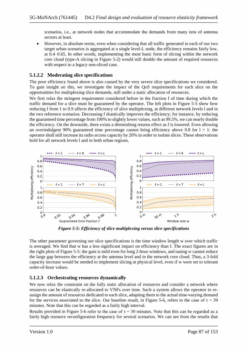
5G-MoNArch (761445) D4.2 Final design and evaluation of resource elasticity framework
Version 1.0 Page 87 of 153
scenarios, i.e., at network nodes that accommodate the demands from many tens of antenna
sectors at least.
• However, in absolute terms, even when considering that all traffic generated in each of our two
target urban scenarios is aggregated at a single level-L node, the efficiency remains fairly low,
at 0.4–0.65. In other words, implementing the most basic form of slicing within the network
core cloud (type-A slicing in Figure 5-2) would still double the amount of required resources
with respect to a legacy non-sliced case.
5.1.2.2 Moderating slice specifications
The poor efficiency found above is also caused by the very severe slice specifications we considered.
To gain insight on this, we investigate the impact of the QoS requirements for each slice on the
opportunities for multiplexing slice demands, still under a static allocation of resources.
We first relax the stringent requirement considered before in the fraction f of time during which the
traffic demand for a slice must be guaranteed by the operator. The left plots in Figure 5-5 show how
reducing f from 1 to 0.9 affects the efficiency of slice multiplexing, at different network levels l and in
the two reference scenarios. Decreasing f drastically improves the efficiency; for instance, by reducing
the guaranteed time percentage from 100% to slightly lower values, such as 99.5%, we can nearly double
the efficiency. On the downside, there exists a diminishing returns effect as f is lowered. Even allowing
an overindulgent 90% guaranteed time percentage cannot bring efficiency above 0.8 for l = 1: the
operator shall still increase its radio access capacity by 20% in order to isolate slices. These observations
hold for all network levels l and in both urban regions.
Figure 5-5: Efficiency of slice multiplexing versus slice specifications
The other parameter governing our slice specifications is the time window length w over which traffic
is averaged. We find that w has a less significant impact on efficiency than f. The exact figures are in
the right plots of Figure 5-5: the gain is mild even for long 2-hour windows, and tuning w cannot reduce
the large gap between the efficiency at the antenna level and in the network core cloud. Thus, a 3-fold
capacity increase would be needed to implement slicing at physical level, even if w were set to tolerant
order-of-hour values.
5.1.2.3 Orchestrating resources dynamically
We now relax the constraint on the fully static allocation of resources and consider a network where
resources can be elastically re-allocated to VNFs over time. Such a system allows the operator to re-
assign the amount of resources dedicated to each slice, adapting them to the actual time-varying demand
for the services associated to the slice. Our baseline result, in Figure 5-6, refers to the case of τ = 30
minutes. Note that this can be regarded as a fairly high interval.
Results provided in Figure 5-6 refer to the case of τ = 30 minutes. Note that this can be regarded as a
fairly high resource reconfiguration frequency for several scenarios. We can see from the results that
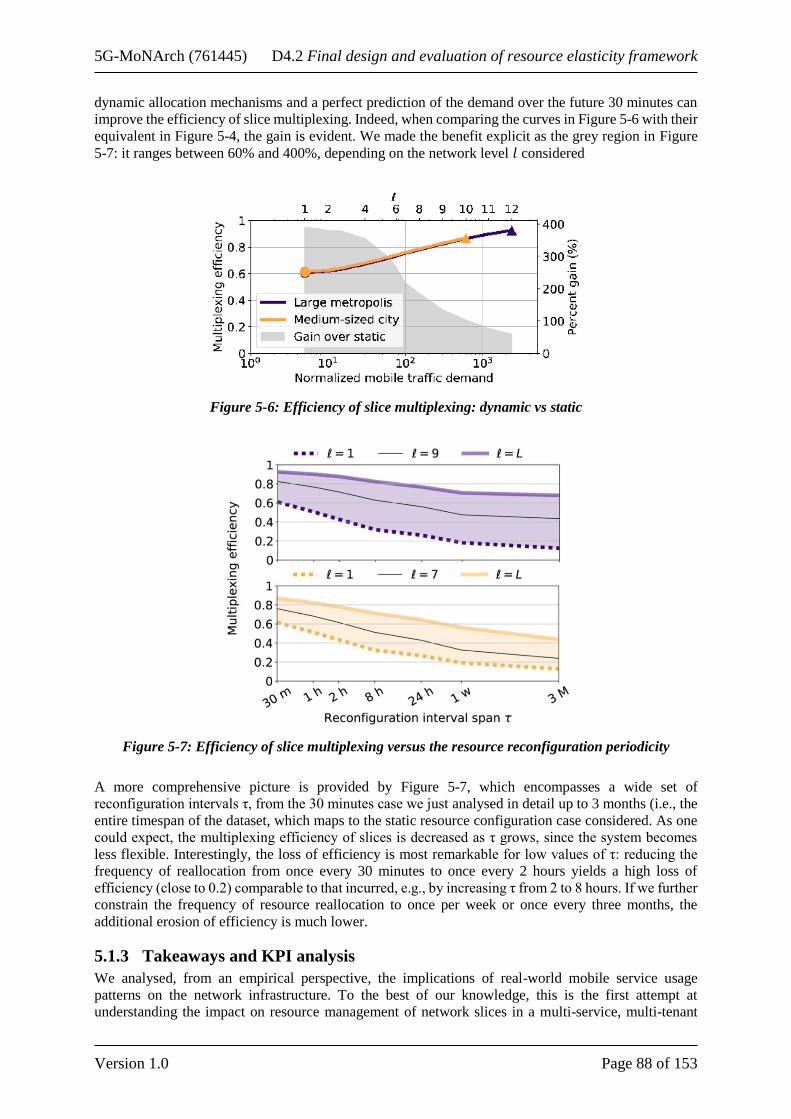
5G-MoNArch (761445) D4.2 Final design and evaluation of resource elasticity framework
Version 1.0 Page 88 of 153
dynamic allocation mechanisms and a perfect prediction of the demand over the future 30 minutes can
improve the efficiency of slice multiplexing. Indeed, when comparing the curves in Figure 5-6 with their
equivalent in Figure 5-4, the gain is evident. We made the benefit explicit as the grey region in Figure
5-7: it ranges between 60% and 400%, depending on the network level 𝑙 considered
Figure 5-6: Efficiency of slice multiplexing: dynamic vs static
Figure 5-7: Efficiency of slice multiplexing versus the resource reconfiguration periodicity
A more comprehensive picture is provided by Figure 5-7, which encompasses a wide set of
reconfiguration intervals τ, from the 30 minutes case we just analysed in detail up to 3 months (i.e., the
entire timespan of the dataset, which maps to the static resource configuration case considered. As one
could expect, the multiplexing efficiency of slices is decreased as τ grows, since the system becomes
less flexible. Interestingly, the loss of efficiency is most remarkable for low values of τ: reducing the
frequency of reallocation from once every 30 minutes to once every 2 hours yields a high loss of
efficiency (close to 0.2) comparable to that incurred, e.g., by increasing τ from 2 to 8 hours. If we further
constrain the frequency of resource reallocation to once per week or once every three months, the
additional erosion of efficiency is much lower.
5.1.3 Takeaways and KPI analysis
We analysed, from an empirical perspective, the implications of real-world mobile service usage
patterns on the network infrastructure. To the best of our knowledge, this is the first attempt at
understanding the impact on resource management of network slices in a multi-service, multi-tenant

5G-MoNArch (761445) D4.2 Final design and evaluation of resource elasticity framework
Version 1.0 Page 89 of 153
network at scale. We retain a number of takeaways, listed next. Although this analysis do not provide
technical solution for improving KPIs it provides an analysis of the cost efficiency in real scenarios.
Multi-service requires more resources. Building a network that is capable of providing different
services (associated to several tenants) will necessarily introduce a decrease in the efficiency of the
resource usage. We quantify this loss in one order of magnitude if considering distributed resources
(such as spectrum), yet the efficiency loss stays as high as 20% even in a fully centralised scenario (i.e.,
a large datacentre in the core network). These figures translate into high costs for the infrastructure
provider who must compensate for them by aggressively monetising on the new business models
enabled by a multi-service scenario (e.g., Network Slice as a Service, Infrastructure as a Service).
Traffic direction is a factor. Uplink and downlink traffic exhibit similar efficiency trends across
network levels, but uplink exacts a much higher efficiency degradation to meet equivalent QoS
requirements. Although uploads account for a small fraction of the overall load, the further reduced
efficiency of uplink may entail real challenges for the operators. Indeed, uplink QoS requirements are
key to specific services with stringent network access needs (e.g., mobile gaming). Even more so, it is
likely that multiple instances of such services belonging to different tenants (e.g., video-gaming
platforms owned by different gaming providers) have to be served in a resource-isolated fashion in
parallel.
Loose service level agreements may not help. Although the slice specifications granted to tenants may
be moderated, the overall efficiency grows only when requirements are very much lowered, up to a point
that they may be not suitable for certain services (needing, e.g., “five nines reliability”, or bandwidth
guarantees over very short time windows).
Dynamic resource assignment must also be rapid. The design of dynamic resource allocation
algorithms is crucial to increase the efficiency of future sliced networks. However, substantial gains will
only be attained if the virtualisation technologies enable a fast enough re-orchestration of network
resources. While current Management and Orchestration (MANO) frameworks provide such
capabilities, intelligent algorithms able to forecast mobile service demands and anticipate resource
reconfiguration are also required, which may be challenging for short timescales. Underestimation of
resources may lead to SLA violations, whereas over-provisioning may harm the economic feasibility of
the system. Artificial intelligence and machine learning are promising techniques to accomplish this
[ENI17, ZPH18] and are being brought into the network management landscape by standards [ENI17].
There is room for improvement. As a final remark, we would like to stress that ours does not pretend
to be a comprehensive analysis, rather one that lays the foundations to a better understanding of the new
trade-offs introduced by network slicing in terms of resource management efficiency. The empirical
bounds we derived represent a starting point for deeper investigations of an unexplored subject, as we
are discussing next, with strong implications for the future generations of mobile networks.
5.2 Slice-aware automatic RAN configuration
A new feature of the 5G systems operating at high frequencies is the use of multiple beam operations
for solving both coverage and capacity requirements. Ensuring service continuity for moving users,
beam management (Layer 2 mechanism) between beams of the serving cell is introduced together with
enhanced scheduling mechanisms. Additionally, dedicated beam forming can be used to address the
diverse service requirements of users. These new techniques can also be used in the context of resource
elasticity and multi slice services.
5.2.1 Detailed description of the solution
This enabler deals with RAN level automatic configurations for scenarios where multiple network slices
are supported at the same time, in addition to varying user traffic. The problem is that the user
concentration of services belonging to network slice with very strict and distinct SLAs (in terms of
throughput and latency) may suddenly appear, move or disappear within the same network area. This
requires a flexible and elastic RAN which allows shifting and concentrating network capacity to areas
where this is needed. The traditional approach for dealing with varying traffic volume is to dimension
the network for busy hour traffic via cell densification or deployment of small cells. However, such
solutions are very costly, since the installed network capacity is unused for most of the time.

5G-MoNArch (761445) D4.2 Final design and evaluation of resource elasticity framework
Version 1.0 Page 90 of 153
The 5G system also introduces a beam-formed access technique which opens the door to another
dimension by making the radio resource allocation more elastic in the spatial domain. Beams are a must
at high frequencies to provide sufficient coverage for a dedicated QoS. For instance, broadcast channel
(BCCH) with robust MCS and low data rate can be radiated with broader beams than user traffic of
services with stringent SLAs. Using narrower beams benefits from the antenna gain and improves the
SINR, and consequently the throughput, of users in the beam spot.
The envisioned beam-driven elasticity solution tries to address the challenges that arise with network
slicing within the confines of a fixed infrastructure and a limited number of RAN resources. More
specifically, the beam and Radio Resource Management (RRM) configurations of a cell or group of
cells in the network will be dynamically adjusted at run time as a function of cell load, number active
slices and spatial traffic distribution.
Due to hardware or interference limitations, users may be served by a single beam at a time and the
scheduling of the beams may need to be done in a sequential manner, i.e. only one beam is active and
serving users with data at any given moment. These two aspects have a direct impact on the QoS of the
users. If the load in a given beam is high, each user will get less resources allocated and thus have a
lower throughput. On the other hand, if only one beam is active in the cell, this can create large delays
for users in the inactive beams which have to wait their turn to be served. These limitations can become
incompatible with the requirements of slices that require a minimum guaranteed bit rate or a maximum
delay (e.g. eMBB, AR/VR applications).
In the following we will explain the proposed solution by means of a simple example scenario in Figure
5-8. In this example, two different network slices (Slice 1 and Slice 2), each mapping a different service
type are active in the same cell that initially uses 12 beams for coverage (4 inner beams and 8 outer
beams). The colour of the users indicates the slice they belong to (AR/VR in red and MBB in blue). The
users belonging to the AR/VR slice are grouped together in a hotspot as part of an organised sightseeing
tour. The MBB users are randomly distributed in all the cell area. Obviously, the AR/VR users need
higher data rates and lower latency than the MBB user but their presence in the cell/network is also
limited (both in space and time).
Figure 5-8: Initial beam configuration
Several ways in shifting capacity within and between the cells and toward the AR/VR/red users are
possible:
(1) By means of adaptive beam configuration
• This approach is similar to well-known mechanisms of load balancing in LTE networks where
the boundary of the cells is virtually pushed in toward the centre of the crowded cell and edge
users are forced to handover to the neighbouring cells.
• In our case, the same can be done by switching off selected beams in the cell where the MBB
users are located. As a result, some of the MBB users will shift to other beams in the cell or to
neighbouring cells. This, in turn, lowers the delay of the active beams (if fewer beams are active

5G-MoNArch (761445) D4.2 Final design and evaluation of resource elasticity framework
Version 1.0 Page 91 of 153
in the cell, this means they can be scheduled more often) and may increase the number of
resources allocated to each user (in the case where MBB users’ handover to other cells).
• This approach comes at the cost of worse SINR for the MBB users as they will be now served
by suboptimal beams.
• In order to make the neighbouring cells even more attractive to MBB users, increase their SINR
and make sure no coverage holes are created by the switching off of beams, the power of
selected beams in neighbouring cells can be increased (referred to in the following as ‘beam
boosting’). This means that the serving cell needs to collect beam measurements from MBB
UEs and communicate to the neighbouring cells via the Xn interface which beams need to be
boosted. Alternately, positioning information of the users could be used (by means of GPS data,
RF fingerprinting, measurement reports from the users [3GPP18-38305]).
• Other limitations that need to be considered are the fact that mixed beams (e.g. beams that serve
MBB and AR/VR users) cannot be switched off and neither can the inner beams which are vital
for the coverage of the cell.
(2) By means of adaptive scheduling: another way of reducing latency of specific services or users is
to schedule beams serving them more often. This has the advantage that it does not impact the coverage
of the cell or its neighbours and trigger unwanted effect. On the other hand, an increase in cell throughput
cannot be directly expected in all cases, as the load is not reduced.
5.2.2 Evaluation scenario and KPIs
The proposed enabler has been tested as a proof of concept in a simplified synthetic 7-site hexagonal
scenario (Figure 5-9). The black circles represent the base station locations and the black lines the
antenna orientation. The AR/VR users (red x) are modelled as a hotspot and carry out Constant Bit Rate
(CBR) traffic. The MBB users (blue circles), are dropped randomly in the cells and are have infinite
buffer traffic. Statistics are collected per cell or per area (e.g. samples of all users in the area given by
the red rectangle in Figure 5-9). Table 5-1 summarises main simulation parameters and sample values.
Figure 5-9: Simulation scenario and user positions

5G-MoNArch (761445) D4.2 Final design and evaluation of resource elasticity framework
Version 1.0 Page 92 of 153
Table 5-1: Main simulation parameters
Parameter name Value
Carrier Frequency 28 GHz
Cell layout 7 site hexagonal, 21 cells, ISD 200m
Bandwidth 400 MHz (40 PRBs of 10MHz each)
Total Output Power 28 dBm per entire bandwidth, 12 dBm per PRB
BS/UE height 10 m /1.5m
Number of MBB users and speed 40 randomly per cell (static)
Number of AR/VR users and speed 5 concentrated in cell (static)
AR/VR data rate 100 Mbps
Simulation time step 10ms
Number of beams per cell 12 (4+8)
Number of beams that can be scheduled per cell 1 or 4
Tx antenna element azimuth beam width 650
Tx antenna element elevation beam width 650
Tx antenna element gain 8dBi
TX Maximum backward/elevation/azimuth
attenuation
30dB
Thermal noise power per PRB -97dBm
Shadowing Not used
Penetration loss 0dB
Pathloss model UMi, LOS, 3GPP TR 38.901
5.2.3 Simulator enhancement description
The enabler will be tested in a proprietary, MATLAB based simplified dynamic system-level simulator.
The simulator does an abstraction of RRM (resources and scheduling) and includes user movement,
changes of system parameters and the reaction of the system on that. It supports multiple layers and
technologies and the system granularity is a configurable time step. Real scenarios can be imported in
the tool or artificial ones can be created (e.g. hexagonal grid).
In addition, 5G beam forming impacts are considered such as the channel model and the SINR
computation. The propagation conditions in high frequency bands are more challenging than in low
frequency bands, making the radio link more susceptible to obstruction. The tool includes a simplified
deterministic channel model which captures the propagation aspects that are relevant for mobility
investigations, specifically that the degradation in the user's signal measurement, caused by fixed
obstacles, is faster for higher carrier frequency and user velocity and depends on the diffraction angle
[ALE+17].
Downlink SINR is typically used for radio link failure detection and throughput calculation. The tool
models of desired and interfering signals are computed by considering the impact of antenna
beamforming at transmitter and receiver. Then, a closed-form expression (approximated by Monte Carlo
method) of average downlink SINR is derived by considering the scheduling probabilities of the users
[UAL18].
In order to support slicing, the simulator was also enhanced with mixed traffic scheduling and
throughout calculations. In the case best effort users (finite or infinite buffer traffic model, MBB slice),
each scheduled user will get fair share of the resources in the cell/beam in every time step. Then, based
on individual SINR and specific mapping curves, a throughput value will be computed for the user. This
means that for the BE (best effort) users, the throughput is directly proportional to the SINR and
inversely proportional to the cell load. In the case of CBR users however, each user will get the exact
number of resources it needs in order to achieve the desired bit rate at the given SINR. A mixed traffic
scheduler will take care to first reserve resources for the CBR users and divide the remaining resources
to the BE users. In the case when beam operations are used, the user’s and beam’s scheduling probability
needs to be computed as input for the SINR and later throughput calculations as explained in [KAL+18].

5G-MoNArch (761445) D4.2 Final design and evaluation of resource elasticity framework
Version 1.0 Page 93 of 153
The beam scheduling probability is a direct measure of the delay the users served by that beam will
experience, i.e. a beam with a larger scheduling probability (pb in the following) will be scheduled more
often and thus users will have a smaller delay.
5.2.4 Simulation results and discussion
In this section, we will look at the performance of the proposed enabler in the scenario described in the
previous section in terms of coverage, cell throughput and beam scheduling delays.
In the simulation scenario, the AR/VR users are placed dropped in a hotspot in cell 1 and served by
beams #5 and #11. The MBB users are randomly dropped in all cells. In the most aggressive form of the
enabler, all outer beams in cell 1 except beam #5 (e.g #1, #2, #3, #4, #6, #7 and #8) can be switched off
in order to force MBB users to move to other beams or cells. The impact of beams being switched off
in cell 1 is presented in Figure 5-10 to Figure 5-13. Unless stated otherwise, each cell can only schedule
one beam at a time, this having an impact on interference levels and scheduling delay.
First, the number of served users in cell 1 and their distribution on beams is impacted (see Figure 5-10).
Initially, cell 1 served 43 users (5 AR/VR and 38 MBB). After switching all outer beams off except
beam #5, 13 MBB users handover to neighbouring cells (6, 8, 9 and 11) while the rest redistribute on
the beams left on in cell 1 (#5 and in the inner beams #1 to #4).
Figure 5-10: User distribution per beams in cell 1 before and after selected beams are switched off
As a result of the user redistribution, the scheduling probabilities of beams in cell 1 also change (see
Figure 5-11). Turned off beams (which serve no users) are not scheduled (e.g. the scheduling probability
is zero) and beams with more users get bigger probabilities assigned. As previously mentioned, a larger
scheduling probability means a lower delay for service of users served by that beam.
As a direct consequence, the SINR of both AR/VR and MBB users is becoming worse after beams being
switched off as users being forced to handover to neighbour cells or suboptimal beams as shown in
Figure 5-12. However, due to the lowered load in the cell and the increased scheduling probabilities, the
throughout in cell 1 is improving as can be seen in Figure 5-13.

5G-MoNArch (761445) D4.2 Final design and evaluation of resource elasticity framework
Version 1.0 Page 94 of 153
Figure 5-11: Beam scheduling probabilities in cell 1 before & after selected beams are switched off
Figure 5-12: SINR CDF of users in cell 1 before and after selected beams are switched off
Figure 5-13: Throughput CDF in cell 1 before and after selected beams are switched off
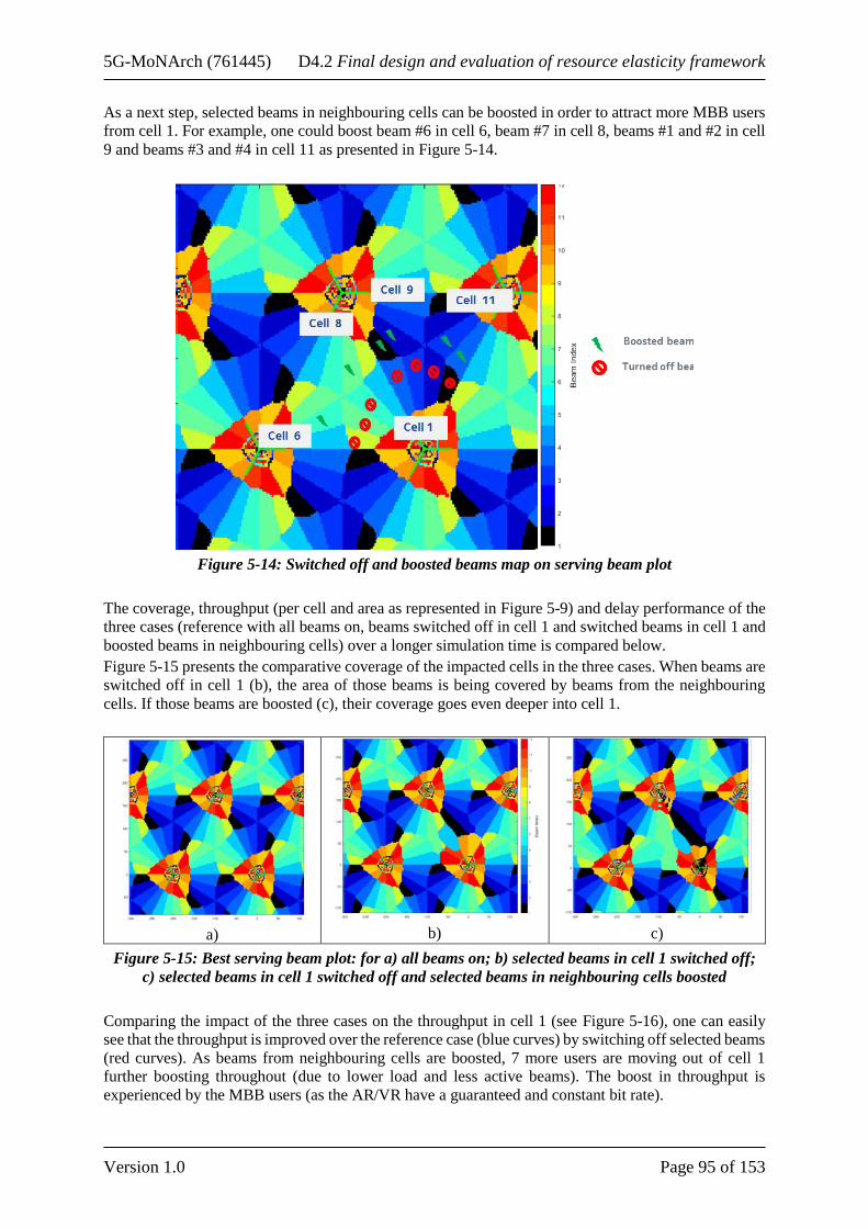
5G-MoNArch (761445) D4.2 Final design and evaluation of resource elasticity framework
Version 1.0 Page 95 of 153
As a next step, selected beams in neighbouring cells can be boosted in order to attract more MBB users
from cell 1. For example, one could boost beam #6 in cell 6, beam #7 in cell 8, beams #1 and #2 in cell
9 and beams #3 and #4 in cell 11 as presented in Figure 5-14.
Figure 5-14: Switched off and boosted beams map on serving beam plot
The coverage, throughput (per cell and area as represented in Figure 5-9) and delay performance of the
three cases (reference with all beams on, beams switched off in cell 1 and switched beams in cell 1 and
boosted beams in neighbouring cells) over a longer simulation time is compared below.
Figure 5-15 presents the comparative coverage of the impacted cells in the three cases. When beams are
switched off in cell 1 (b), the area of those beams is being covered by beams from the neighbouring
cells. If those beams are boosted (c), their coverage goes even deeper into cell 1.
a)
b)
c)
Figure 5-15: Best serving beam plot: for a) all beams on; b) selected beams in cell 1 switched off;
c) selected beams in cell 1 switched off and selected beams in neighbouring cells boosted
Comparing the impact of the three cases on the throughput in cell 1 (see Figure 5-16), one can easily
see that the throughput is improved over the reference case (blue curves) by switching off selected beams
(red curves). As beams from neighbouring cells are boosted, 7 more users are moving out of cell 1
further boosting throughout (due to lower load and less active beams). The boost in throughput is
experienced by the MBB users (as the AR/VR have a guaranteed and constant bit rate).

5G-MoNArch (761445) D4.2 Final design and evaluation of resource elasticity framework
Version 1.0 Page 96 of 153
Figure 5-16: Throughput CDF in cell 1 in the three cases
Of course, by shifting load from cell 1 to the neighbouring cells, the throughput of these cells is
decreasing due to the higher load, lowered SINR of served users and lower scheduling probabilities. The
most impact can be seen in cell 9 which take most of the handed over users (see Figure 5-17).
Figure 5-17: Throughput CDF in the three cases in cells (top left to bottom right 6, 8, 9 and 11
A benefit of shifting users to neighbouring cells is the decreased scheduling delay for beams in cell 1,
which is especially beneficial for the AR/VR users served by beams #5 and #11 but also for MBB users
(see Figure 5-18). The scheduling delay is indirectly proportional to the serving beam’s scheduling
probability and is computed assuming a TTI of 1ms. Switching off beams in cell 1, cuts the delay of the
AR/VR users by half (from 6 ms to 3.3ms) while a further boosting of neighbour cells only bring a gain
of 0.4ms. The average delay in the cell is also cut by 50% by the enabler.

5G-MoNArch (761445) D4.2 Final design and evaluation of resource elasticity framework
Version 1.0 Page 97 of 153
Figure 5-18: Scheduling delay per beam in cell 1 in the three cases
In case more beams can be active at the same time in a cell, both intra- and inter-cell interference
increases negatively impacting the users’ SINR. On the other hand, delay is reduced per beam and cell
as users need to wait less until scheduled. This can be seen in Figure 5-19 where up to 4 beams could
be scheduled at the same time. If compared to the above case (see Figure 5-18, where only one beam
was scheduled at a time), the delay of the beams serving the AR/VR users is lower in all cases: 1.6ms
and 3.9ms respectively as compared to the previous 6ms and 10.6ms. Applying the enabler, further
reduces this delay per beam and average per cell.
Figure 5-19: Scheduling delay per beam in cell 1 in the three cases, up to 4 beams scheduled
simultaneously
User throughput which is a function of both SINR and number of allocated resources, is further
improved when allowing more beams to be scheduled simultaneously in all cases in the cell of interest
(cell 1) and neighbour cells as can be seen in Figure 5-20 and Figure 5-21.

5G-MoNArch (761445) D4.2 Final design and evaluation of resource elasticity framework
Version 1.0 Page 98 of 153
Figure 5-20: Throughput CDF in cell 1 in the three cases, up to 4 beams scheduled simultaneously
Figure 5-21: Throughput CDF in the three cases in cells (top left to bottom right) 6, 8, 9 and 11, up
to 4 beams scheduled simultaneously
In the following we will compare the performance of the first method (i.e. adaptive beam configuration)
with the second one, adaptive scheduling. In particular, we tried to match the scheduling delay of beams
5 and 11 of the cell 1 (that served the delay sensitive AR/VR users) by forcing the scheduling
probabilities of these beams to be equal to the values obtained when using the first method. This means
that, in the case of adaptive scheduling, beams 5 and 11 with have a higher scheduling probability and
the other beams in the cell, smaller ones than in the reference case. As before, the higher the scheduling
probability, the lower the delay experienced by that beam. As a side effect, the MBB users served on
beams 5 and 11 will also be scheduled more often thus resulting in higher experienced throughput.

5G-MoNArch (761445) D4.2 Final design and evaluation of resource elasticity framework
Version 1.0 Page 99 of 153
The resulting throughput in cell 1 is presented in Figure 5-22 and Figure 5-23 below, for the cases when
one and 4 beams are scheduled simultaneously. As mentioned in the previous section, when using the
adaptive scheduling method, users are not shifted between cells so the load in the cell remains constant.
By forcing higher beams scheduling probabilities for AR/VR beams, we boost the throughput of the co-
served MBB users (some of them experiencing a boost of 600%) but we also decrease the throughput
of all other MBB users since the beams serving them are now served for a smaller portion of the time.
Figure 5-22: Throughput CDF in cell 1 in all cases
Figure 5-23: Throughput CDF in cell 1 in all cases, up to 4 beams scheduled simultaneously
Another side effect is the impact on interfering to neighbouring cells that comes from the enforced
scheduling probabilities. The effect of all schemes can be compared using area throughput (Figure 5-24
and Figure 5-25) that considers samples from all users in the red rectangle, as depicted in the previous
section.

5G-MoNArch (761445) D4.2 Final design and evaluation of resource elasticity framework
Version 1.0 Page 100 of 153
Figure 5-24: Throughput CDF in selected area in all cases
Figure 5-25: Throughput CDF in selected area in all cases, up to 4 beams scheduled
simultaneously
The rectangular area is constructed in such a way that it contains all UEs of cell 1 (the cell of interest)
and cells 6, 8, 9 and 11 which are impacted by changed in the beam patterns. The area also contains
other users from other surrounding cells that are not at all impacted by the changed to beam patterns or
adaptive scheduling. In total, samples from 378 users are gathered and plotted, but only 183 belong to
the cells impacted by the changes. Also, in the case of the adaptive beam configuration, load is shifted
from cell 1 (where throughput of all users increases and delay decreases) to neighbouring cells where
the throughout is slightly degraded, so the two trends even each other out. In the case of adaptive
scheduling, as load is not shifted at all between cell, the impact is even smaller. This outcome is also
not surprising if we keep in mind that no resources of any kind have been added.

5G-MoNArch (761445) D4.2 Final design and evaluation of resource elasticity framework
Version 1.0 Page 101 of 153
5.2.5 Conclusions and link with KPIs
The enabler tested two different methods in a simplified touristic city scenario: adaptive beam
configuration and adaptive scheduling.
Both methods manage to significantly reduce the delay of the users in an implicit or explicit manner,
either by decreasing the number of beams that are to be scheduled (i.e. via the adaptive beam
configuration approach) or by imposing beam scheduling constraints in the cell (i.e. via the adaptive
scheduling approach).
In terms of throughput, the adaptive beam configuration method brings more gain for all users in the
targeted cell. This method is in fact a load balancing mechanism which also means that the gain in one
cell produces degradation of performance in the neighbouring cells. Also, as this method changes
physical coverage of the cells, it has more impact on the area and the overall coverage which can become
spotty, so the beam boost component should be used with care.
Since the adaptive scheduling method keeps the changes local to the cell of interest, there is little to no
impact to the neighbouring cells. However, this also means the load is constant in the cell and throughput
gains cannot be achieved. Both throughput and delay can be mapped to reliability.
Ultimately, both methods have advantages and disadvantages and picking the most appropriate one
comes down to scenario specifics like hotspot size and movement, coverage stability and weight of
specific KPIs.
5.3 Game theory approach to resource assignment
In the context of an elastic MANO system, the resource assignment problem can be modelled in several
ways. In this section, we apply a game-theoretical model to this problem.
5.3.1 Network slicing model
We consider a wireless network consisting of a set of resources B (the base stations or sectors) shared
by a set of network slices O (each operated by a different tenant). At given point in time, the network
supports a set of active users U (the customers or devices), which can be subdivided into subsets Uob,
Ub and Uo, corresponding to the users of slice o at base station b, the users at base station b, and the
users of slice o, respectively. We consider that the association of users with base stations is fixed (e.g.,
by a pre-specified user association policy) and let b(u) denote the base station that user u is (currently)
associated with.
5.3.1.1 Resource allocation model
Following a similar approach as [CBV+17], in our model each slice o is allocated a network share so
(corresponding to its budget) such that ∑ soo∈𝒪 = 1. The slice is at liberty to distribute its share
amongst its users, assigning them non-negative weights (corresponding to the bids):wu for u ∈ Uo, such
that ∑ wu ≤ sou∈𝒰ℴ .
We let wo = (wu: u ∈ 𝒰ℴ) be the weights of slice o, w = (wu: u ∈ U) those of all slices and w−o =
(wu: u ∈ U ∖ Uo) the weights of all users excluding those of slice o. We further let lb(w) = ∑ wuu∈𝒰𝒷
denote the load at base station b, dbo(wo) = ∑ wuu∈𝒰𝒷
ℴ the aggregate weight of slice o at b, and
abo(w−o) = ∑ wuu∈𝒰𝒷∖𝒰𝒷
ℴ the aggregate weight of all other slices (excluding o) at b. We shall allocate
each user a fraction of the base station's resources in proportion to her weight 𝑤𝑢.
We let 𝑐𝑢 denote the achievable rate for user u, defined as the product of (i) the average rate per resource
unit achieved by the user, and (ii) the total amount of resources available at the base station. Note that
this depends on the modulation and coding scheme selected for the current radio conditions, which
accounts for noise as well as the interference from the neighbouring base stations. Following similar
analyses in the literature [GLK14], we shall assume that 𝑐𝑢 is fixed for each user at a given time.
We further let 𝑟𝑢 denote the rate allocated to user u. Under our model, 𝑟𝑢 is given by 𝑐𝑢 times the fraction
of the base station's resources allocated to the user. Given that users are allocated a fraction of resources
proportional to their weights, we have that is a function of the weights w given by:

5G-MoNArch (761445) D4.2 Final design and evaluation of resource elasticity framework
Version 1.0 Page 102 of 153
ru(𝐰) =wu
∑ wvv∈𝐔b(u)
cu =wu
lb(u)(𝐰)cu.
When implementing the proposed resource allocation mechanism, a slice may assign a non-zero weight
to some users while others may be dropped. To decide the setting of the users' weights, we assume that
each slice o is aware of the aggregate weight of the other tenants at each base station, i.e., abo(𝐰−o). It
is worth noting that for the mechanism under study we have that (i) a slice only sees the aggregate weight
of the other slices, and hence can learn very limited information about the other slices; in particular, the
weights of each tenant are not disclosed, and (ii) the mechanism needs to store very limited data; indeed,
it is sufficient to keep the total load of each base station, as a tenant can obtain abo(w−o) by simply
subtracting its weight from the base station's load. Such information is already considered within the
network slicing management system defined by 3GPP [3GPP18-28531], and hence should be readily
available.
In order to avoid the indeterminate form resulting from having all the weights at a base station equal to
0 in the above equation, we will require weights to exceed a fixed lower bound (i.e., wu ≥ δ, ∀u). This
bound can be arbitrarily small; indeed, in practice it should be set as small as possible, to allow slices
the highest possible flexibility while avoiding zero weights. Accordingly, in the rest of the discussion
we assume that δ is so small that its effect can be neglected, except where this assumption is required to
prove the existence of a Nash Equilibrium.
In the case where a slice o is the only one with users at a given base station b, such a slice would simply
set wu to the minimum possible value for these users, allowing them to receive all the resources of this
base station while minimising the consumed share To avoid dealing with this special case, hereafter we
shall assume that all base stations have users from at least two slices. Note that this assumption is made
to simplify the expressions and discussion and does not limit the generality of our analysis and
algorithm, which indeed supports base stations with all users from the same slice.
5.3.1.2 Slice utility
Network slices may support services and customers with different needs or may wish to differentiate the
service they provide from competing slices. To that end, we assume that each slice has a private utility
function, Uo, that reflects the slice's performance according to the preferences and needs of its users.
The slice utility consists of the sum of the individual utilities of its users, 𝑈𝑢, i.e.
𝑈𝑜(𝐰) = ∑ 𝑈𝑢(𝑟𝑢(𝐰))u∈𝑈𝑜 .
For inelastic traffic, we assume each user u requires a guaranteed rate γu, hereafter referred to as the
user's minimum rate requirement. In this section we adopt the former model, which aims at providing
users with a guaranteed rate, and thus is aligned with the Guaranteed Bit Rate (GBR) class of 3GPP.
𝑈𝑢 (𝑟𝑢 (w)) = ϕufu(ru(𝐰)), for 𝑟𝑢 (w) ≥ 𝛾𝑢,
where fu(⋅) is a concave utility function associated with the user, and 𝜙𝑢 is the relative priority of user
u (where 𝜙𝑢 ≥ 0 and ∑ 𝜙𝑢𝑢∈𝑈𝑜 =1 ). The relative priorities reflect the importance that users are given by
the tenant of their slice; they drive, jointly with the load at the respective base stations, the weights
assigned to the users, which in turn determine the rate allocation.
Note that the above utility function is only defined for rates above the minimal requirement, as
performance degrades drastically if this guarantee is not met. Note also that the above definition includes
elastic traffic, which corresponds to the special case γu = 0; thus, the results of this document apply to
mixes of elastic and inelastic traffic.
While most of our results hold for arbitrary 𝑓𝑢(⋅) functions, in some cases we will focus on the following
widely accepted family of utility functions (see α −fairness [MW00]):
𝑓𝑢(𝑟𝑢) = {
(𝑟𝑢)1−𝛼𝑜
(1 − 𝛼𝑜), 𝛼𝑜 ≠ 1
log(𝑟𝑢) , 𝛼𝑜 = 1
where the αo parameter sets the level of concavity of the user utility functions, which in turn determines
the underlying resource allocation criterion of the slice. Particularly relevant cases are 𝛼𝑜 = 0
(maximum sum), 𝛼𝑜 = 1 (proportional fairness), 𝛼𝑜 = 2 (minimum potential delay fairness) and 𝛼𝑜 → ∞ (max-min fairness).
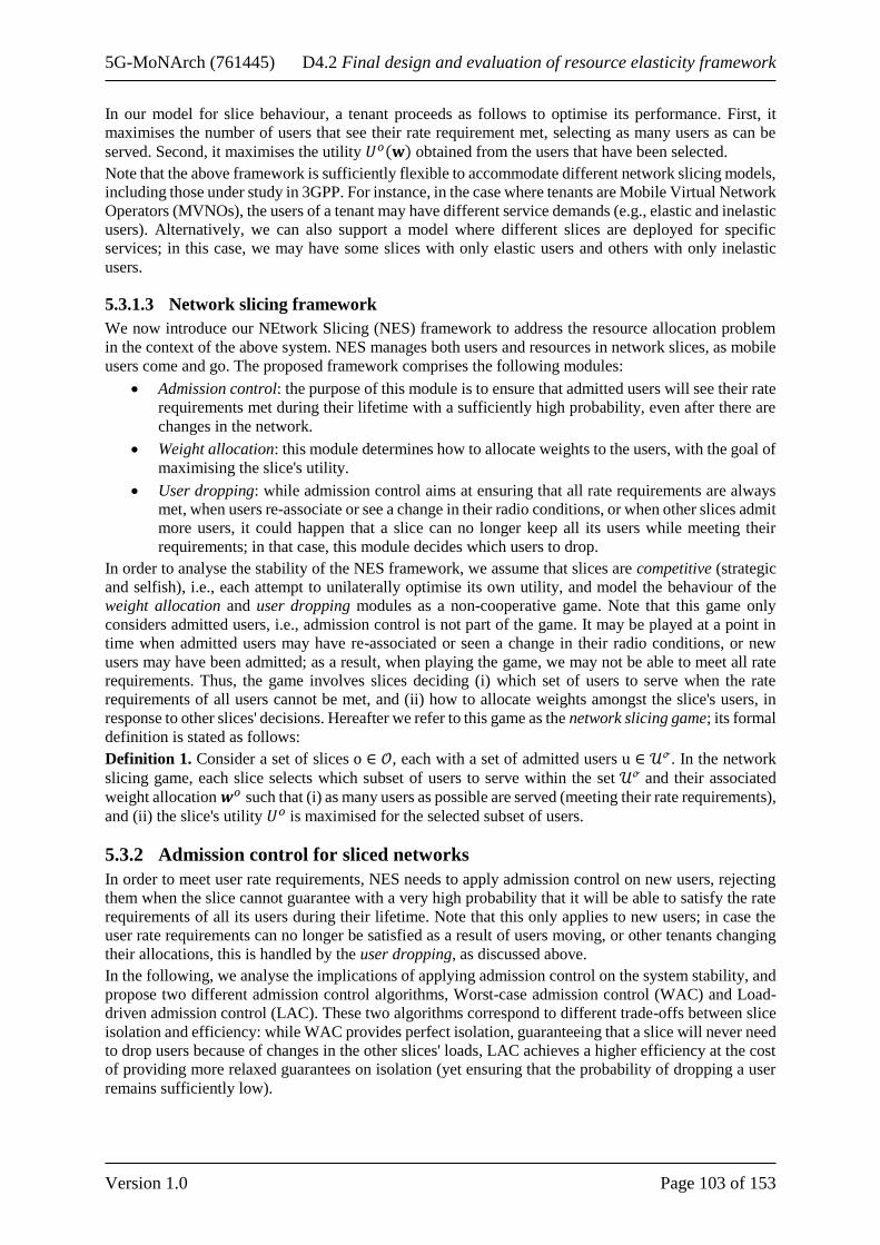
5G-MoNArch (761445) D4.2 Final design and evaluation of resource elasticity framework
Version 1.0 Page 103 of 153
In our model for slice behaviour, a tenant proceeds as follows to optimise its performance. First, it
maximises the number of users that see their rate requirement met, selecting as many users as can be
served. Second, it maximises the utility 𝑈𝑜(𝐰) obtained from the users that have been selected.
Note that the above framework is sufficiently flexible to accommodate different network slicing models,
including those under study in 3GPP. For instance, in the case where tenants are Mobile Virtual Network
Operators (MVNOs), the users of a tenant may have different service demands (e.g., elastic and inelastic
users). Alternatively, we can also support a model where different slices are deployed for specific
services; in this case, we may have some slices with only elastic users and others with only inelastic
users.
5.3.1.3 Network slicing framework
We now introduce our NEtwork Slicing (NES) framework to address the resource allocation problem
in the context of the above system. NES manages both users and resources in network slices, as mobile
users come and go. The proposed framework comprises the following modules:
• Admission control: the purpose of this module is to ensure that admitted users will see their rate
requirements met during their lifetime with a sufficiently high probability, even after there are
changes in the network.
• Weight allocation: this module determines how to allocate weights to the users, with the goal of
maximising the slice's utility.
• User dropping: while admission control aims at ensuring that all rate requirements are always
met, when users re-associate or see a change in their radio conditions, or when other slices admit
more users, it could happen that a slice can no longer keep all its users while meeting their
requirements; in that case, this module decides which users to drop.
In order to analyse the stability of the NES framework, we assume that slices are competitive (strategic
and selfish), i.e., each attempt to unilaterally optimise its own utility, and model the behaviour of the
weight allocation and user dropping modules as a non-cooperative game. Note that this game only
considers admitted users, i.e., admission control is not part of the game. It may be played at a point in
time when admitted users may have re-associated or seen a change in their radio conditions, or new
users may have been admitted; as a result, when playing the game, we may not be able to meet all rate
requirements. Thus, the game involves slices deciding (i) which set of users to serve when the rate
requirements of all users cannot be met, and (ii) how to allocate weights amongst the slice's users, in
response to other slices' decisions. Hereafter we refer to this game as the network slicing game; its formal
definition is stated as follows:
Definition 1. Consider a set of slices o ∈ 𝒪, each with a set of admitted users u ∈ 𝒰ℴ. In the network
slicing game, each slice selects which subset of users to serve within the set 𝒰ℴ and their associated
weight allocation 𝒘𝑜 such that (i) as many users as possible are served (meeting their rate requirements),
and (ii) the slice's utility 𝑈𝑜 is maximised for the selected subset of users.
5.3.2 Admission control for sliced networks
In order to meet user rate requirements, NES needs to apply admission control on new users, rejecting
them when the slice cannot guarantee with a very high probability that it will be able to satisfy the rate
requirements of all its users during their lifetime. Note that this only applies to new users; in case the
user rate requirements can no longer be satisfied as a result of users moving, or other tenants changing
their allocations, this is handled by the user dropping, as discussed above.
In the following, we analyse the implications of applying admission control on the system stability, and
propose two different admission control algorithms, Worst-case admission control (WAC) and Load-
driven admission control (LAC). These two algorithms correspond to different trade-offs between slice
isolation and efficiency: while WAC provides perfect isolation, guaranteeing that a slice will never need
to drop users because of changes in the other slices' loads, LAC achieves a higher efficiency at the cost
of providing more relaxed guarantees on isolation (yet ensuring that the probability of dropping a user
remains sufficiently low).

5G-MoNArch (761445) D4.2 Final design and evaluation of resource elasticity framework
Version 1.0 Page 104 of 153
5.3.2.1 Nash equilibrium existence
A critical question is whether the network slicing game possesses a Nash Equilibrium (NE), i.e., there
exists a choice of users and associated weight allocation w such that no slice can unilaterally modify its
choice to improve its utility. In the following, we analyse the requirements on admission control policies
in order to ensure that a NE exists after admission control is applied. Note that, if the game does not
have a NE, strategic slice behaviour may lead to system instability affecting the practicality of the
proposed approach.
The following theorem shows that if admission control cannot ensure that slices can satisfy the rate
requirements of all their users, the network slicing game may not have a NE. The proof of the theorem
exhibits a case where instability arises when there is no weight allocation such that the rate requirements
of all the users of a given slice are met given feasible allocations for the other slices. Note that in a
dynamic setting such a situation could arise, when a slice initially admits users for which the
requirements are feasible, and subsequently other slices admit additional users to their slice, making
some of the users in the first slice infeasible.
Theorem 1. When slices cannot satisfy all of their users’ rate requirements, the existence of a NE cannot
be guaranteed for the network slicing game.
The problem identified by the above theorem can be overcome by applying an admission control scheme
that avoids such situations. According to the following theorem, a NE exists as long as admission control
is able to guarantee that a slice can satisfy the rate requirements of all its users under any feasible weight
allocation of the other slices (including future allocations when possibly new users may have been
admitted). Note that in this case the resulting game focuses on maximising slice utilities while meeting
the rate requirements of all users. This result implies that, as long as proper admission control is
implemented and ensures that rate requirements can always be satisfied, the stability of the system can
be guaranteed.
Theorem 2. Suppose admission control ensures that, for any feasible weight allocation of the other
slices, each slice o has a weight allocation wo such that its users’ rate requirements are met. Then, the
network slicing game has a (not necessarily unique) NE.
Note that the above theorem guarantees the existence of a NE when all slices are elastic; indeed, elastic
slices have a rate requirement equal to 0, and therefore their rate requirements can always be satisfied.
In the following, we propose two alternative admission control policies (one more aggressive and one
more conservative) that aim at ensuring that the conditions given by Theorem 2 are met. Note that it is
up to the tenant to choose and customise its admission control strategy, and hence each tenant may
independently apply its own admission control policy.
5.3.2.2 Worst-case admission control (WAC)
The WAC policy is devised to ensure that the rate requirements of all users are always met,
independently of the behaviour of the other tenants. To that end, under the WAC policy a slice admits
users as follows: it conservatively assumes it has access to only a fraction so of resources at each base
station and admits users only if their requirements can be satisfied with these resources.
Given that a user needs a fraction γu/cu of the base station's resources to meet her rate requirement, this
policy imposes that for slice o the following constraint is satisfied at each base station b:
∑𝛾𝑢𝑐𝑢≤ so,
u∈𝒰𝒷ℴ
The WAC policy aims at ensuring that the above is satisfied at all times. However, even if this condition
holds when a new user is admitted, it may be subsequently violated upon changes in the slice, e.g., due
to mobility of users or changes in their 𝑐𝑢.
To provide robustness against such changes, we add a guard band to the equation above aimed at
ensuring that the condition will continue to hold with high probability after any changes.
Thus, a slice admits a new user request as long as the following holds
∑𝛾𝑢𝑐𝑢≤ 𝜌𝑤 ⋅ 𝑠𝑜,
𝑢∈𝒰𝒷ℴ

5G-MoNArch (761445) D4.2 Final design and evaluation of resource elasticity framework
Version 1.0 Page 105 of 153
b
b
where 𝜌𝑤 < 1 parametrises the guard band: the smaller this parameter, the larger the guard band. In
practice, this parameter may be set to different values by different slices based on the slice specifics,
such as the fluctuations of 𝑐𝑢 or user association (where larger fluctuations will require a larger guard
band) or the desired level of assurance to its users (stricter guarantees will require a larger guard band).
In the following, we analyse the properties of WAC under the assumption that the above equation is
satisfied with this policy. The theorem below shows that, as long as this condition is satisfied, a slice
will always be able to meet its users' rate guarantees independent of the setting of the other slices. Thus,
a high degree of protection to the choices and changes in other slices is provided.
The theorem also shows that if the slice deviates from the proposed policy, it is not protected from the
other slices' choices, implying that this policy represents a necessary condition to provide protection.
Theorem 3. Consider a slice o with users having rate requirements γo = (γu : u ∈ U o), then the following
hold:
If the above equation is satisfied, there exists at least one weight allocation wo such that ∀u ∈ U o ru(w)
≥ γu, for any feasible allocation of the other slices’ aggregate weights ao.
If above equation is not satisfied, slice o is not protected, as there is a feasible ao allocation such that
slice o is not able to meet the rate requirements of its admitted users.
Note that combining this result with Theorem 2, it follows that a NE exists when all slices run WAC.
Indeed, the above theorem ensures that a slice can find an allocation that meets the rate requirements of
all its users for any feasible ao, which comprises all the possible allocations of the other slices w−o.
5.3.2.3 Load-driven admission control (LAC)
While the WAC policy protects a given slice from the others, it may be overly conservative in some
cases where base stations are lightly loaded or where some slices are unlikely to use resources at certain
base stations. In those cases, one may opt to be more aggressive in admitting users without running
significant risks. To this end, we propose the LAC policy, where a slice measures the current load across
base stations and performs admission control decisions based on the measured loads (assuming that they
will not change significantly).
The following theorem provides a basis for the design of the LAC policy. It gives a necessary and
sufficient condition that has to be satisfied to meet the rate requirements of the slice's users, given the
current weight allocations of the other slices. This constraint is shown to be less restrictive than the one
imposed by LAC, implying that LAC (potentially) allows the admission of more users than WAC.
Theorem 4. Consider a slice o comprising users with rate requirements γo = (γu : u ∈ U o), and suppose
the aggregate weight of the other slices is given by ao. Then, a weight allocation wo that meets slice o’s
rate requirements exists if and only if the following is satisfied: where U o is the subset of users of slice
o associated with base station b, according to the given user association policy. Moreover, if the rate
requirements satisfy (4), then the above condition is satisfied
The central idea of the LAC policy is as follows. Upon receiving a request of a new user u with a rate
requirement γu, slice o assesses the current ao values in the network and checks whether (5) would be
satisfied with the new user. According to the theorem, as long as (5) is satisfied, the rate requirements
can be met if the ao values do not change. However, in practice ao may change due to the response of
the other slices to slice o, or to changes in the other slices (e.g., the admission of new users). We shall
address this uncertainty by following a similar approach to WAC: when admitting a new user, we verify
that (5) is satisfied with a sufficiently large guard band, i.e., where ρl < 1 is the parameter providing the
guard band for LAC. Note that, in addition to other considerations, in this case the setting of ρl will need
to account for observed statistical fluctuations of ao, larger fluctuations requiring a larger guard band.
The following theorem shows that, as long as the chosen value for ρl is sufficiently conservative, LAC
is effective in guaranteeing that the rate requirements of all users are met.
Theorem 5. There exists a ρl value sufficiently small such that the rate requirements of all the users of
slice o can be met independent of how the other slices change their weights

5G-MoNArch (761445) D4.2 Final design and evaluation of resource elasticity framework
Version 1.0 Page 106 of 153
5.3.3 Performance evaluation
We next evaluate the performance of NES via simulation. Unless otherwise stated, the mobile network
setup of our simulator follows the IMT-A evaluation guidelines for dense “small cell” deployments
[ITU09-M21351], considering a network with 19 base stations disposed in a hexagonal grid layout with
3 sectors, i.e., |B|=57. User mobility follows the Random Waypoint (RWP) model. The users arrive to
the network following a Poisson Process with intensity λ arrivals/sec, and their holding times are
exponentially distributed. Users' SINR is computed based on physical layer network model specified in
[ITU09-M21351] (which includes path loss, shadowing, fast fading and antenna gain) and user
association follows the strongest signal policy. The achievable rate for a user u, 𝑐𝑢, is determined based
on the thresholds reported in [3GPP15-36213]. Unless otherwise stated, the rate requirement of the
inelastic users is set to 𝛾𝑢=0.5 Mbps, we have 𝛼𝑜= 1 for all slices, there are 5 slices in the network
with equal shares, the arrival rate is 𝜆 = 5 (equally split among slices) and the average holding time is 1
minute. In the simulations, we consider both slices with mixed traffic of different types and as well as
slices dedicated to one specific traffic type.
5.3.3.1 Network utility
We first analyse the network utility achieved by NES as compared to the two benchmark solutions:
Socially Optimal Allocation (SO): If slices were to share their utility functions with a central authority,
one could in principle consider a (share-constrained) allocation of weights (and resources) that optimises
the overall performance of the network, expressed in terms of the network utility U (w).
Static Slicing Allocation (SS): By static we refer to a complete partitioning of resources based on the
network shares so, o ∈ O. In this setting, each slice o receives a fixed fraction so of each resource, which
is shared among its users proportionally to their weights.
To ensure that the rate requirements of admitted users are always met, we adopt the WAC admission
control policy with 𝜌𝑤 = 1 and suppress user movements yielding changes in base station associations
and/or 𝑐𝑢 values. To analyse the impact of inelastic traffic, we vary the fraction of inelastic traffic
arrivals, θ, yielding an arrival rate of 𝜃𝜆 for inelastic users and of (1- 𝜃) 𝜆 for elastic ones. The results,
depicted in the Figure below, show that (i) NES outperforms very substantially SS, providing very high
gains, and (ii) it performs optimally, very close to the SO. Moreover, this holds independently of the
mix of elastic and inelastic users present in the network.
Figure 5-26: Performance of NES in terms of network utility as compared to the two benchmark
allocations (SS and SO)

5G-MoNArch (761445) D4.2 Final design and evaluation of resource elasticity framework
Version 1.0 Page 107 of 153
5.3.3.2 Blocking probability
In addition to improving the performance of admitted users, one of the key advantages of the dynamic
resource allocation implemented by NES is that it allows admitting more users while meeting their rate
requirements. In order to assess the achieved improvement, we evaluate the blocking probability (i.e.,
the probability that a new user cannot admitted) under NES versus SS.
For NES, we consider the two admission policies proposed above (WAC and LAC), while for SS we
apply the policy given in [RTN97]. For all settings, we drop users based on the MaxSubsetSelection
algorithm, and adjust the guard bands to ensure that the probability of dropping an admitted user is no
more than 1%.To increase the offered load sufficiently so that we can observe the behaviour of the
blocking probability, we set 𝛾𝑢 =1 Mbps and an average holding time of 2 minutes.
The results are given in the figure below as a function of the fraction of inelastic user arrivals 𝜃. They
show very high gains over SS for both approaches (WAC and LAC), and confirm that, by behaving
more aggressively, LAC is able to admit many more users than WAC.
Figure 5-27: Blocking probability for new arrivals for the two policies proposed and the SS
benchmark
Analysis with respect to the 5G-MoNArch KPIs
This enabler focuses mostly on the cost efficiency of the network, by providing a better resource
assignment in presence of multi-slice deployment. If used in conjunction with elastic VNF such as the
one presented in Chapter 6, it will also contribute to enhance the other KPIs relevant for network
elasticity, such as rescuability and graceful degradation.
5.4 Slice-aware computational resource allocation
5.4.1 Background
The efficient and flexible utilisation of the computational resources is an integral part of the 5G
networks, since many 5G NFs are expected to be virtualised and, hence, they will consume resources
from a shared/cloudified environment. A chained set of physical and virtualised network functions
(VNF) will serve as a network slice (NS), while multiple slices should be supported by an infrastructure
owner (operator). In this context, although an initial allocation of resources to the VNF of the different
network slices will be performed, a dynamic allocation process is needed to deal with random
fluctuations of computational and traffic load over time. According to the current 3GPP standardisation
activity for 5G, this process could take place during the run-time phase of the lifecycle of a slice instance

5G-MoNArch (761445) D4.2 Final design and evaluation of resource elasticity framework
Version 1.0 Page 108 of 153
and could be part of the functionality assigned to the NSMF entity in the 5G architecture [5GM-D22].
Practically, computational, storage and network resources, are controlled by virtual infrastructure
managers in a dynamic and efficient way, in a sense, that the VNFs utilise the minimum required
resources, guaranteeing a target performance for the subject slices. Although for this allocation, we can
theoretically assume infinite resources at a centralised cloud, it is not the case when edge cloud/fog
nodes undertake the processing load. From a more general perspective, it is also important the
computational resources to be utilised efficiently in a proactive way, i.e., in case that unpredicted
additional processing power is requested, the system will be able to address the request. This approach
in resource allocation is aligned with the principles of applying network resource elasticity, as defined
in [5GM-D41]. In line with the targeted resource elasticity KPI for the project, the approaches described
in this section, are expected to:
• have indirectly positive impact on the cost efficiency gain, since the approaches target at
reducing/optimising the utilisation of the computational resources. The analysis in Section 5.4.3
considers also this perspective, by defining an optimisation function that includes the cost of
executing VNF in different computation machines.
• slightly affect the service creation time, since the time needed for the execution of the allocation
algorithm described in Section 5.4.2.3 is executed every time a service requires the set-up of a
slice.
• have direct impact on the resource utilisation efficiency since the optimisation criterion for the
proposed approaches is to maximise the utilisation of the computational resources.
5.4.2 Efficient resource utilisation
5.4.2.1 Problem formulation
The problem of allocating VNFs that compose slices to computation resources (or computation
machines) can be described with the aid of the following notation:
• Let a set of computation machines 𝑚 = 1,2,3,… ,𝑀, that refer to processing machines on which
the VNFs can run, and a set of services 𝑛 = 1,2,3, … ,𝑁.
• Each service consists of a set of VNFs
• Each 𝑉𝑁𝐹𝑣𝑛 , 𝑣 = 1,2,3,… , 𝑉, 𝑛 = 1,2,3,… , N can be allocated on an arbitrary computation
machine 𝑚 of a set 𝑀𝑠(𝑀𝑠 ⊆ 𝑀), at a corresponding setup time 𝑆𝑣𝑛𝑚, and be processed for a
given uninterrupted processing time 𝑃𝑣𝑛𝑚.
• Let also 𝐶𝑛 be the completion time of service 𝑛, or 𝐶𝑛 = 𝑆𝑣𝑛𝑚 + 𝑃𝑣𝑛𝑚. Also, max1≤𝑛≤𝑁
(𝐶𝑛) is the
makespan, i.e., the total time needed to complete the execution of all the VNFs (or the time
needed for completing the “longer” service).
The objective is to devise a compromise schedule that minimises the makespan. Mathematically:
𝑚𝑖𝑛 max1≤𝑛≤𝑁
(𝐶𝑛)
subject to:
𝑆𝑇𝑣𝑛 + ∑[𝑥𝑣𝑛𝑚(𝑆𝑣𝑛𝑚 + 𝑃𝑣𝑛𝑚)]
𝑀
𝑚=1
≤ 𝑆𝑇(𝑣+1)𝑛 +∑[𝑥(𝑣+1)𝑛𝑘(𝑆(𝑣+1)𝑛𝑚 + 𝑃(𝑣+1)𝑛𝑚)]
𝑚
𝑘=1
∑ 𝑥𝑣𝑛𝑚
𝑀
𝑚=1
= 1 with ∀v, 𝑛
𝑆𝑣𝑛𝑚 = 𝑆𝑣𝑛 𝑥𝑣𝑛𝑚 with ∀𝑣, 𝑛,𝑚
Where:
• 𝑥𝑣𝑛𝑚 equals 1 if 𝑉𝑁𝐹𝑣𝑛 is finished on computation machine k, and 0 otherwise
• 𝑆𝑇𝑣𝑛 starting epoch of setup VNF for service 𝑛
• 𝑆𝑇𝑣𝑛𝑚 equals 𝑆𝑇𝑣𝑛 if 𝑣 is finished on machine 𝑚, and 0 otherwise

5G-MoNArch (761445) D4.2 Final design and evaluation of resource elasticity framework
Version 1.0 Page 109 of 153
The inequality above indicates the operation sequence constraint, while the two equations indicate that
each computation machine m = 1,2,3,… ,𝑀 can process at most one VNF at a time, and at most one
VNF of each service 𝑛 can be processed at a time, respectively. Note that the operation sequence
constraint is an important aspect of this formulation, since each service can be seen as a flow of packets
which must pass through various VNFs, e.g., the functions in the protocol stack that edit/affect the
packets serially.
5.4.2.2 Proposed approach
According to the computational complexity theory, the problem above belongs to the class of problems
that are NP-hard in the strong sense. An optimisation problem is NP-hard (in the strong sense) if its
decision version is NP-complete (in the strong sense). The proof that the decision problem is NP-
complete has been provided in detail by Garey and Johnson [GJ79]. Another (simple) way to prove that,
is through graph theory, since the above problem can be mapped to the graph colouring problem. This
mapping to the graph-colouring analogous also triggers the design of graph-based solutions that can
approximate the optimal solution of the problem. This is the main motivation of the work proposed in
this document. In view of this, a key probabilistic optimisation approach, inspired by the behaviour of
real ants searching for food, namely the Ant Colony Optimisation (ACO) [MGL04 is adopted on top of
a representation graph.
The representation graph composed for resolving the problem is built as follows:
We assume a complete directed graph 𝐺 = (𝑉, 𝐸) where the vertexes represent VNFs: 𝑉 ={(𝑣1, 𝑛1),… , (𝑣𝑉 , 𝑛𝑁)} . The allocation of the computation resources to a service is considered
successful, if the execution time of all the VNFs that compose this service is below a pre-defined
threshold, which guarantees acceptable quality; otherwise an outage occurs. The execution time
(measured in time units) is used as a weight for the edges of the graph, according to the following rule:
• If two VNFs, represented by vertices, 𝑣𝑎 , 𝑣𝑏 can be executed concurrently (no operation
sequence constraint) the weight in the edge that connects the two vertices (both directions)
equals 𝜔(𝑣𝑎, 𝑣𝑏) = |𝑃𝑎𝑛𝑎𝑚𝑎− 𝑃𝑏𝑛𝑏𝑚𝑏
|, where 𝑎 ≠ 𝑏, 𝑛𝑎, 𝑛𝑏 ∈ 𝑁, and 𝑚𝑎 ,𝑚𝑏 ∈ 𝑀𝑇.
• If two VNFs, represented by vertices 𝑣𝑎 , 𝑣𝑏 , cannot be executed concurrently (operation
sequence constraint is applied) the weight in the edge that connects the two vertices in the
direction that respects the constraint (let 𝑣𝑎 → 𝑣𝑏) equals 𝜔(𝑣𝑎 , 𝑣𝑏) = 𝑃𝑏𝑛𝑏𝑚𝑏, where 𝑛𝑏 ∈ 𝑁
and 𝑚𝑏 ∈ 𝑀𝑇(note that for the opposite direction the edge does not exist in the graph).
For approximating the optimal solution, the ACO is applied as follows:
Ants are treated as “coloured agents”, where each one is carrying a unique colour. When an ant visits a
node “paints” the node with this colour. In the resource allocation scenario that we examine, this means
that the ant allocates the same computation machine to all visited nodes (i.e., VNFs), which will then
consist a part of this ant’s solution 𝐿 (i.e, a path in the graph with the nodes coloured with the same
colour). Overall, the redefined parameters of the ACO are:
• 𝑀 = the total number of ants (i.e., machines).
• 𝑚 = the index to an ant.
• 𝐿𝑚 = {𝑣𝑖, 𝑣𝑗, … , 𝑣𝐿𝑙𝑒𝑛𝑚 }, representing a solution of ant 𝑚, after 𝐿𝑙𝑒𝑛
𝑚 steps (after the colouring of
𝐿𝑙𝑒𝑛𝑚 nodes)
• 𝑡𝑎𝑏𝑢𝑚 = the “tabu list” of ant 𝑚, to prevent it from colouring the same node more than once.
• 𝑟 = the evaporation rate used in the ACO procedure. It represents how fast the topology changes
and hence how fast acquired knowledge by past ACO iterations fades.
• 𝑑𝑖𝑗 = 𝜔(𝑣𝑖 , 𝑣𝑗), which for simplicity is normalised to a [1-100] scale describing 100 distinct
time units
• 𝜂𝑖𝑗 = the attractiveness of moving from vertex 𝑣𝑖 to 𝑣𝑗. It indicates the a priori desirability of
the move, i.e., here, the desirability of assigning the same colour to 𝑣𝑗, provided that it has been
already allocated to 𝑣𝑖.

5G-MoNArch (761445) D4.2 Final design and evaluation of resource elasticity framework
Version 1.0 Page 110 of 153
𝜂𝑖𝑗 =1
𝑑𝑖𝑗=
1
𝜔(𝑣𝑖 , 𝑣𝑗)
• 𝐶𝑚 = the estimated cost that derives from ant 𝑚’s route. Here, it is the total execution time
resulted by the path from ant 𝑚
• 𝛥𝜏𝑖𝑗𝑚 = the pheromone deposited by ant 𝑚’s 𝑖 → 𝑗 move:
𝛥𝜏𝑖𝑗𝑚 = {
1
𝐶𝑚 , 𝑖𝑓 𝑏𝑜𝑡ℎ 𝑖 𝑎𝑛𝑑 𝑗 𝑤𝑒𝑟𝑒 𝑣𝑖𝑠𝑖𝑡𝑒𝑑 𝑏𝑦 𝑎𝑛𝑡 𝑚
0, 𝑖𝑓 𝑛𝑜𝑡
• 𝜏𝑖𝑗 = the trail level or amount of pheromone deposited for moving from 𝑣𝑖 to 𝑣𝑗. It indicates
how proficient has been in the past the colouring of 𝑣𝑗 given the same colouring of 𝑣𝑖 and, thus,
indicates the a-posteriori desirability of this move.
𝜏𝑖𝑗(𝑡) = (1 − 𝑟)𝜏𝑖𝑗(𝑡 − 1) +∑𝛥𝜏𝑖𝑗𝑘
𝑁
𝑘=1
• 𝛼 = the level of importance of 𝜏, 1 ≥ 𝛼 ≥ 0.
• 𝛽 = the level of importance of 𝜂, 𝛽 ≥ 1.
• 𝑝𝑖𝑗𝑚
= the transition probability that ant 𝑚 will move from 𝑣𝑖 to state 𝑣𝑗. It depends on both 𝜂
and 𝜏.
𝑝𝑖𝑗𝑚 =
𝜏𝑖𝑗𝛼𝜂𝑖𝑗
𝛽
∑ 𝜏𝑖𝑗𝛼𝜂𝑖𝑗
𝛽𝑎𝑙𝑙 𝑓𝑒𝑎𝑠𝑖𝑏𝑙𝑒 𝑗 𝑠𝑡𝑎𝑡𝑒𝑠
The finding of the maximum possible size of 𝐿𝑚 is driven by an iterative procedure inside the NSMF
function. It is actually a check that is performed to guarantee that for each service the maximum number
of time units is not exceeded. Measuring the number of outages out of all the scheduled VNFs that
compose 𝐿𝑚, the NSMF gets an estimation of the average Outage Probability (𝑃𝑜𝑢𝑡), which, in turn, is
compared to a maximum acceptable threshold. The optimisation problem is expressed as the
minimisation of a sum of weights:
min𝑊(𝑣𝑖, 𝑣𝑗) 𝑤ℎ𝑒𝑟𝑒 𝑣𝑖, 𝑣𝑗 𝜖 𝑉
s.t., 𝐿𝑙𝑒𝑛𝑚 < 𝐿, ∀𝑚, 𝑚 𝜖 𝑀
where 𝑊 is a 𝑉𝑥𝑉 matrix of all weights, and 𝐿 the maximum number of time units for the execution of
all the VNFs.
5.4.2.3 Resource allocation algorithm
Having provided the terminology and basic idea behind the application of the ACO theory for this
resource allocation problem, we describe the proposed algorithm in Figure 5-28.
We demonstrate an example to assess the number of iterations needed for the ACO to reach a close-to-
optimal solution. We considered that 𝑀 = 20 machines are available, and 40 VNFs have to be executed,
where each one of them needs a number of computation units. With no loss of generality, the requests
for computation units are normalised to a [1-100] scale. We allow the algorithm to run for multiple
evaluation runs (x axis in Figure 5-29), and we observe the algorithm’s behaviour in terms of reducing
the required execution time units (depicted as: best cost in y axis of Figure 5-29). As it can be observed
in Figure 5-29, the algorithm gradually approaches a stable solution, due to its self-learning nature.
Starting from a relatively high cost in the first iteration the algorithm manages to steadily reduce the
total cost down to around 50 units. This reduction indicates the discovery of constantly better paths in
the graph.
To further examine the behaviour of the proposed approach we performed tests with different values for
the evaporation rate variable (denoted by 𝑟 in the analysis). This variable represents the level that the
algorithm learns from previous allocations, and its values are the percentage of information from a
previous allocation that is lost. We present results for 𝑟 = 10% and 𝑟 = 1% in Figure 5-30. As it can
be observed, after 500 iterations (lest part of Figure 5-30) the performance is not that stable, and the

5G-MoNArch (761445) D4.2 Final design and evaluation of resource elasticity framework
Version 1.0 Page 111 of 153
learning aspect has small affect to it. However, after 5000 iterations (right part of Figure 5-30) the impact
of learning is presented, and the performance for 𝑟 = 1% is much more stable and closer to optimal.
- Initialisations: 𝐿𝑙𝑒𝑛𝑚 = 𝐿, 𝑉, 𝑀, 𝑟, 𝛼, 𝛽, and 𝑃𝑜𝑢𝑡
while 𝑉 ≠ {} repeat
- Create the 𝑑𝑖𝑗 matrix ∀(𝑖, 𝑗) ∈ 𝑉 - Create a first solution & estimate a reference cost
- Estimate 𝜂𝑖𝑗 and initialise 𝜏𝑖𝑗 ∀(𝑖, 𝑗) ∈ 𝑉 while evaluation runs > 0
for ant 𝑚 = 1:𝑀 - Initialise starting node 𝑖 of each ant 𝑚 - Add node 𝑖 to 𝐿𝑚and 𝑡𝑎𝑏𝑢𝑚 while ant’s solution < 𝐿 - Estimate all transition probabilities 𝑝𝑖𝑗𝑛
𝑚
- Add node 𝑣𝑖𝑛 into 𝐿𝑚 based on 𝑝𝑖𝑗𝑛
𝑚
- Append node 𝑣𝑗𝑛 to 𝑡𝑎𝑏𝑢𝑚
end while
- Estimate 𝐶𝑚 end for
- Update trail levels 𝜏𝑖𝑗(𝑡) ∀(𝑖, 𝑗) ∈ 𝑉 - Update: evaluation runs = evaluation runs - 1
end while
- Estimate 𝑃𝑜𝑢𝑡 with the least 𝐶𝑚 ever
- Update: 𝐿𝑚 until 𝑃𝑜𝑢𝑡 < threshold - Remove subset that compose 𝐿𝑚 from 𝑉 end while
Figure 5-28: Algorithm: ACO-based resource allocation
Figure 5-29: Convergence time for the proposed algorithm

5G-MoNArch (761445) D4.2 Final design and evaluation of resource elasticity framework
Version 1.0 Page 112 of 153
Figure 5-30: The impact of imperfect feedback (learning) from previous resource allocations
5.4.3 Performance degradation model
Beyond the resource allocations that assume all the information deterministic (as the one explained
above), where the number of requests and resources are known, here we examine the problem from the
cost-effective perspective, including in the analysis a probabilistic fashion of some of the input
parameters.
Let the following set of definitions:
• A period of 𝑇 slots (𝑡 = 1,2,3,… , 𝑇 ), for which we investigate the optimal (based on an
optimisation function) allocation of a number of VNFs to a set of computation machines
• In the time-slot 𝑡 = 0 the allocation is decided for all the time slots (𝑡 = 1,2,3,… , 𝑇)
• Let the set of different VNFs be indexed by 𝑛 = 1,2,3… , 𝑁
• Let the set of available machines are indexed by 𝑚 = 1,2,3,…𝑀
• For the duration of one slot multiple VNFs of the same type can be curried by the same machine,
and more precisely, at the time-slot 𝑡 the machine 𝑚 is able to carry 𝐶𝑛𝑚𝑡 VNFs of type 𝑛
• For a time-slot 𝑡, machine 𝑚, and VNF 𝑛, the allocation decision is denoted by 𝑑𝑛𝑚𝑡 ∈ {0,1}
• Let in the period of 𝑇 slots, the request is to run 𝑠𝑛 = ∑ 𝑠𝑛𝑡𝑇𝑡=1 instances of VNF 𝑛
The target is to minimise the performance degradation when VNF are executed, i.e.,
𝐿 = ∑(𝑙𝑛 ∙ 𝑔 (𝑠𝑛 − ∑∑𝑑𝑛𝑚𝑡 ∙ 𝐶𝑛𝑚𝑡
𝑇
𝑡=1
𝑀
𝑚=1
) + ℎ(𝑑𝑛))
𝑁
𝑛=1
Where,
• 𝑙𝑛 : performance degradation of failing to run an instance of VNF 𝑛 in the specific time period
• 𝑔(𝑥) = 𝑥 if 𝑥 > 0, 𝑔(𝑥) = 0 otherwise
• ℎ(𝑑𝑛) : a function describing the performance degradation due to the execution of VNF 𝑛 in
the decided machines (e.g., extra delay due to the location of the machine)
Since in a realistic scenario the requests (referring to the requested number of instances for each VNF 𝑛
to be executed, i.e., 𝑠𝑛) are not known, we can assume that we have an indication on the expected number
of requests based, for instance, on network monitoring and study of past measured data. In this case, the
expected performance degradation is as follows:
⟨𝐿⟩ = ∑ ∑ 𝑃(𝑠𝑛|𝐼)
∞
𝑠𝑛=1
(𝑙𝑛 ∙ 𝑔 (𝑠𝑛 − ∑∑𝑑𝑛𝑚𝑡 ∙ 𝐶𝑛𝑚𝑡
𝑇
𝑡=1
𝑀
𝑚=1
) + ℎ(𝑑𝑛))
𝑁
𝑛=1
where, 𝑃(𝑠𝑛|𝐼) is the probability distribution function of the requests conditioned on whatever
information 𝐼 is available at the function that performs the resource allocation, which in this case in the
NSMF.

5G-MoNArch (761445) D4.2 Final design and evaluation of resource elasticity framework
Version 1.0 Page 113 of 153
If the available information 𝐼 is the mean values of 𝑠𝑛, ∀𝑠𝑛, 𝑛 𝜖 𝑁, denoted here by ⟨𝑠𝑛⟩, then problem
is coined to be a problem of finding the maximum entropy of 𝑃(𝑠𝑛|𝐼).
Based on Shannon Maximum Entropy Principle we have:
𝐻 = − ∑ 𝑃(𝑠𝑛|𝐼)
∞
𝑠𝑛=1
log (𝑃(𝑠𝑛|𝐼))
under the constraint of ⟨𝑠𝑛⟩ = ∑ 𝑠𝑛𝑃(𝑠𝑛|𝐼)∞𝑠𝑛=1
The solution can be based on the Lagrange method using as Lagrange Multipliers the following:
⟨𝑠𝑛⟩ = ∑ 𝑠𝑛𝑃(𝑠𝑛|𝐼)
∞
𝑠𝑛=1
=1
𝑒𝜆𝑛 − 1
and thus, using the general maximum entropy distribution, we have:
𝑃(𝑠𝑛|𝐼) = (1 − 𝑒−𝜆𝑛)𝑒−𝜆𝑛𝑠𝑛
𝑃(𝑠𝑛|𝐼) =1
⟨𝑠𝑛⟩ + 1(
⟨𝑠𝑛⟩
⟨𝑠𝑛⟩ + 1)
⟨𝑠𝑛⟩
To illustrate this derivation, we provide Figure 5-31, where the 𝑃(𝑠𝑛|𝐼) is quantified for different values
of ⟨𝑠𝑛⟩.
Figure 5-31: The relation between the expected number of instances for each VNF and the
distribution probability of all the requests
Based on this result the expected degradation can be provided by
⟨𝐿⟩ = ⟨𝑠𝑛⟩ (⟨𝑠𝑛⟩
⟨𝑠𝑛⟩ + 1)
𝑥𝑛
where,
𝑥𝑛 = ∑∑𝑑𝑛𝑚𝑡 ∙ 𝐶𝑛𝑚𝑡
𝑇
𝑡=1
𝑀
𝑚=1
The formula provided above, can be exploited further by decision-based resource allocation algorithms
and optimisations that target at minimising the performance degradation when computational resources
are dynamically allocated to VNFs.
5G-MoNArch (761445) D4.2 Final design and evaluation of resource elasticity framework
Version 1.0 Page 114 of 153
5.5 Profiling of computational complexity of RAN
Section 4.5 the elastic resource management, needs to estimate the total radio and computational
capacity before allocating the available resources to each slice. The radio capacity is the estimated total
network throughput using the available radio resource pool. The computational capacity, however, is
the processing power to process different VNFs. The elastic resource management algorithm has to
estimate the total processing capacity and the required processing capacity for each VNF. Then, it can
map the available computational resources to each VNF of each slice.
A practical approach to study the computational complexity of VNFs is to measure the processing time
of each VNF based on different inputs. Finally, the processing time as the function of inputs can be
modelled based on the measurements and used in elastic resource management algorithm. The
computational model for the physical layer has been already presented in the previous deliverables. In
the same research path, this section presents the measurement results for L2 and L3. In the next
deliverable, these results will be complete by a closed-form models.
The testbed for profiling the computational complexity has four key elements, which are:
• the commercial UE: LG Nexus 5, UE Cat. 4, Release rel10 operating in Long Term Evolution
(LTE) FDD Band 7 (2.66 GHz downlink, 2.54 GHz uplink).
• eNB: Open Air Interface (OAI) [OAI] running on a machine with Intel Core i7-4790 CPU @
3.60GHz and 16 GB RAM. Its operating system is Kubuntu 16.04 LTS with Kernel version
4.4.0-130-low-latency. The processor has four physical cores, eight logical threads, and 8 MB
of Cache Memory and supports instruction set extensions SSE4.1/4.2, AVX 2.0. The eNB is
operating in 5 MHz bandwidth, which means there are 25 PRBs available.
• USRP B210 module: a Software-Defined Radio (SDR) module that is used on eNB for RF
transmissions,
• EPC: Openair-cn is used as EPC (Evolve Packet Core) running HSS (Home Subscriber Server),
MME (Mobility Management Entity) and S/P-GW (Serving/PDN (Packet Data Network)
Gateway) on a separate machine.
OAI is an open-source software-based implementation of the LTE system spanning the full protocol
stack of 3GPP standard. While the previous study in has used OAI simulation tools “dlsim” and “ulsim”,
which emulate PDSCH (Physical Downlink Share Channel) and PUSCH (Physical Uplink Share
Channel) respectively, the present study uses the OAI eNB operating over the air and while a COTS UE
is connected. Two command line option provided by the OAI eNB are of special interest here.
The original measurement mechanism of accumulates statistics over the whole runtime and presents a
report right before eNB software is terminated. However, in the framework of this profiling and for the
realisation of experimental optimisation, the measurements are reported via UDP (User Datagram
Protocol) to a different application running also in a different machine. For the sake of simplicity, the
instantaneous reports are accumulated and then reported at configurable intervals. The profiling
measurement is done by full buffer traffic (i.e. when all 25 PRBs are allocated).
Just like any other measurement procedure of a physical quantity, measuring the processing time of a
computational task might affect the subject of the measurement. In this study, this concern is of special
interest because eventually measurement probes become part of the system as processing times of
selected functionalities are to be reported to a controller node rather than being removed after evaluation.
The addition of probe points and reporting point into the different VNFs might affect both the actual
value of the measurement and also the performance of the VNF under measurement. Time
measurements are taken with the inclusion of probe points right before and right after of the selected
process in question.
The resolution offered by any of the three methods is sufficient. As the size of concerned tasks (in the
range of µs) are relatively large compared to taking measurement itself, the issues with cost and
reliability can be neglected. As a result, all three methods display good characteristics. In Figure 5-32,
measurements for modulation block using these three methods are presented, regarding mean or
variance, no substantial difference exists among them.

5G-MoNArch (761445) D4.2 Final design and evaluation of resource elasticity framework
Version 1.0 Page 115 of 153
Figure 5-32: Comparison of time measurement methods – modulation processing time
5.5.1.1 Profiling over the air PHY layer
Measurements for the profiling of PHY layer functions (i.e., encoding, scrambling, and modulation)
over the air operation is compared to the previous investigation that present results for simulated
environment [5GM-D41]. Also, the profiling is extended to the upper layers. The measurements of PHY
network functions in downlink are captured while running a speed test via a smartphone application for
each of the MCS index. It worth noting that the readings, in which the UE is not allocated the total
available number of PRBs (i.e. 25 PRBs) are removed from our measurements. Figure 5-33 shows the
average processing time for the encoding, scrambling and modulation in downlink direction.
Figure 5-33: The average processing time for PHY layer network functions
It is important to notice that the measurements for encoding have a relatively high variance. For instance,
the reading for MCS index 28 has the mean processing time of about 50us with the standard deviation
of 35us. Further investigation is planned to consider the processing time for the different subprocess
involved, i.e. segmentation, turbo encoding, interleaving and rate matching. With the analysis of those
measurements is expected on the one hand to identify a set of parameters leading to a partitioning of the
measurement space where the different groups get characterised for having a particular average
processing time and a smaller variance.
5.5.1.2 Profiling at MAC/RLC/PDCP layers
There are two key functionalities at higher layers regarding the data flow in downlink direction: a) the
scheduling process place between Media Access Control (MAC) and Radio Link Control (RLC), b) the
user data transfer from PDCP (Packet Data Convergence Protocol) to RLC.

5G-MoNArch (761445) D4.2 Final design and evaluation of resource elasticity framework
Version 1.0 Page 116 of 153
The downlink scheduling routine is active in each subframe, and it includes functionalities that execute
entirely at the MAC layer as well as a set of functionalities that execute at both MAC and RLC. While
it is easy to measure the processing time of former functionality in MAC, the separation of the lather
functionalities in the current OAI implementation is not possible without adding additional processing
delay. Hence, the measurements of the processing time of these functionalities are the combined
processing time of MAC and RLC layer.
The tasks performed solely at MAC are those carried at the “pre-processor module” OAI, which is the
central scheduling entity for uplink/downlink. This unit is responsible for:
• Scheduling radio resources to UEs (e.g. number byte per UE per subframe and per carrier)
• Pre-allocation of PRBs,
• Gathering Partial Marginalisation Multiple Input Multiple Output (PM/MIMO) layer
information,
• Providing beamforming (TM7-10),
• Return a priority list for “deterministic” allocation of Downlink Control Information (DCI) and
physical resources carried out by LTE mechanism described above. It operates on state of
network and reorder according priorities and “pre”-allocate resources.
The downlink scheduling process involving RLC layer functionalities are:
• MAC to RLC Status Indication: this function retrieves RLC logical channel queue status during
the MAC scheduling operation. It is typically invoked during the pre-processor step in order to
determine the number of bytes that are to be scheduled per-user in a particular subframe. It is
also called just prior to requesting a target number of bytes from the RLC.
• MAC to RLC Data Request: this function requests downlink Service Data Units (SDUs) from
RLC for transport channel multiplexing. A particular number of bytes are requested, and the
closest amount is returned to MAC.
In Figure 5-34, a measurement capture for the downlink scheduling is presented. Each point in the plots
represents the average of 50 consecutive samples in contrast to the MAC layer where samples are taken
every subframe (1ms). The measurements represent a capture while running speed test via the
smartphone app during nearly a minute, 1.300 intervals * 50ms/interval = 65.000 ms.
Figure 5-34: Profiling results for MAC-RLC downlink scheduling
Out of the plot, a very rough relation of the processing time vs the operational load (in term of utilised
subframes) is presented in Table 5-2. Measurement were also taken limiting the maximum downlink
MCS index obtaining virtually same results.
For the user data transfer from PDCP to RLC, the main functionality involved is the RLC to PDCP data
request initiated at PDCP layer whenever a PDCP data request occurs. This function transfers a downlink
SDU from PDCP to RLC for a particular signalling or data radio bearer and it is called from the PDCP
entity and routed inside the RLC to the desired unit for segmentation and queuing.

5G-MoNArch (761445) D4.2 Final design and evaluation of resource elasticity framework
Version 1.0 Page 117 of 153
PDCP data requests are executed not only in the user plane but also in the control plane, however the
number of calls corresponding to control plane are very small compared to the ones of the user plane.
For the data plane case, the arrival of a G-PDU (GTP encapsulated user Plane Data Unit) at the S1
interface initiates the PDCP data request. Such event is asynchronous, and it might happen zero or more
times per subframe.
Table 5-2: MAC downlink processing time and operational load
% of utilised sub-frames approx. Avg. processing time (microseconds)
100% full buffer operation 6
60% 4-5
40% 4
20% 3
< 20% 0.6
Figure 5-35 presents the profiling of PDCP using iperf tool [Iperf] to generate UDP traffic in downlink
direction setting a 10 Mbps bandwidth and with a test duration of 60 seconds. Results has shown an
average processing delay or about 0.854µs and having sporadically very large processing time peaks of
several hundreds of µs. The middle plot in this figure also confirm that this functionality is being
executed more than once per subframe as one call per subframe would mean a total of 60.000 calls while
more than 100.000 measurements are captured. Measurements has shown that the under full buffer
operation PDCP data request occurs between 0 and 4 times per subframe with an average of 1.701 calls
per subframe.
Looking deeper to the statistic of the collected measurements, it shows in upper part the number of calls
below a given processing time in steps from 1us to 14 µs. There can be seen that 65% of the calls fall
below 1µs, and almost 99% of them below 2µs.
Figure 5-35: Processing time PDCP data requests
In the next step, the same profiling measurement is going to be repeated to study the effect of PRB
utilisation and the selected MCSs on the MAC and PDCP. After complete gathering of the
measurements, a mathematical model is going to be fitted to using machine learning techniques (Lasso
regression [Tib96]).
Online profiling and learning of computational complexity: The computational complexity of the
network functions in addition to their functionality is highly dependent on the implementations
techniques and it may change from one VNF provider to another one as well as one version to another.
The background OS process and the performance of virtualisation platform (i.e., the container or virtual
machine) also effect the processing time.
On the same research path, AI-based solutions (Lasso, Support Vector Machine (SVM), or
reinforcement learning [MB12]) can learn (or adopt) the computational performance of VNFs based on
the reported input parameters and the measured processing times for any new VNFs. The numeric results
above can provide a baseline for further studies. However, we suggest profiling the processing time of
each VNF to be monitored using the methodology described above. Using the Lasso regression
techniques as it has shown in [5GM-D41], a polynomial estimation is fit to the readings in each interval
and the coefficients are updated.

5G-MoNArch (761445) D4.2 Final design and evaluation of resource elasticity framework
Version 1.0 Page 118 of 153
6 Elastic network functions
While in the previous Chapter 4 and Chapter 5 we focused on the cross-slice and intra-slice aspects of
network elasticity, in this chapter we target the third dimension of elasticity, namely computational
elasticity.
We are currently observing the softwarisation of communication networks, where network functions are
translated from monolithic pieces of equipment to programs running over a shared pool of
computational, storage, and communication resources. As the amount of this resources might vary over
time, in this chapter we propose specific algorithms that introduce resource awareness to softwarised
network functions. While these proposals are just possible outcomes of the application of computational
elasticity to NFs, we expect that this paradigm will be one of the fundamental pillars of future, beyond
5G networking. So, the enablers described in this chapter are residing in the Network and Control Layer,
defining an elastic approach to RAN Scheduling (Section 6.1) and Elastic Rank Control (Section 6.2).
Figure 6-1: Innovations on elastic resource management on top of 5G-MoNArch architecture
6.1 Elastic RAN scheduling
In this section, we present our system model and formulate the optimisation problem that will drive the
computational-aware scheduling of the users. The model is inspired in Long Term Evolution Advanced
(LTE-A) but is applicable to any cellular system.
We consider a typical cloud-computing platform that is serving a set 𝒮 of Resource Access Points
(RAPs). The amount of resources devoted to the baseband processing for these RAPs is given by the
computational capacity 𝐶 . We let 𝑈 denote the set of users in the system and 𝑈𝑠 the set of users
associated with RAP𝑠 ∈ 𝒮. Each RAP has a number 𝐵 of resource blocks.
Time is divided into Transmission Time Intervals (TTIs) and scheduling decisions are performed for
each TTI 𝑡. We assume that each user sees the same SNR level in all resource blocks at each TTI. Within
the constraints imposed by the channel quality of a user, we may select among different MCSs; we
denote the set of possible MCS schemes available for user 𝑢 at a given TTI as 𝑀𝑢(𝑡). Note that the
computational load is a function of the MCS and the SNR; we let 𝑐𝑢𝑚(𝑡) denote the computational load
incurred to decode a resource block for user 𝑢 under MCS 𝑚 ∈ 𝑀𝑢 at TTI 𝑡 (given the user’s channel
at that time).
Elastic RAN scheduling
Elastic Rank Control

5G-MoNArch (761445) D4.2 Final design and evaluation of resource elasticity framework
Version 1.0 Page 119 of 153
Following the above, at each TTI a central scheduler decides (i) the mapping of users to resource blocks,
and (ii) the users’ MCS, with the goal of improving the overall system performance under the available
computational capacity. In particular, following, we impose that the aggregate computational load in the
system (given by the individual loads 𝑐𝑢𝑚(𝑡)) cannot exceed the computational capacity 𝐶.
In the above system, scheduling and MCS selection are driven by the decision variable 𝑥𝑢𝑏𝑚(𝑡), which
indicates that resource block b is assigned to user 𝑢 with MCS 𝑚 at TTI 𝑡. Based on this variable, the
rate received by user 𝑢 at TTI 𝑡 is given by:
𝑟𝑢(𝑡) =∑ ∑ 𝑥𝑢𝑏𝑚(𝑡)𝑟𝑢𝑚(𝑡),
𝑚∈ℳ𝑢(𝑡)
𝑏∈ℬ𝑠(𝑢)
where ℬ𝑠(𝑢) is the set of resource blocks at user 𝑢’s RAP, ℳ𝑢(𝑡) is the set of MCS options available
for user 𝑢 at time 𝑡 (according to the radio conditions at that time) and 𝑟𝑢𝑚(𝑡) is the rate provided to
user 𝑢 by one resource block with MCS 𝑚.
The average rate of user 𝑢 is given by 𝑅𝑢, which is updated at each TTI by the following exponentially
smoothed average:
𝑅𝑢(𝑡 + 1) = (1 − 𝛼)𝑅𝑢(𝑡) + 𝛼𝑟𝑢(𝑡),
where 𝛼 is the smoothing factor and 𝑟𝑢(𝑡) is the rate received by user 𝑢 at TTI 𝑡
Our goal in this system is to maximise performance in terms of Proportional Fairness (PF), which leads
to the following optimisation problem:
The above formulation optimises performance under the constraints that the consumption of
computational resources does not exceed the available capacity, each resource block is only assigned
once, a user can employ only one MCS and we cannot select a higher MCS than the one allowed by
current radio conditions. Note that these constraints do not force that all resource blocks available in a
RAP are used; indeed, in some cases it may be better to leave some resource blocks unused to free
computational resources that can be used by other resource blocks employing higher MCS, achieving in
this way a more efficient use of the system resources.
As the proportional fairness criterion considered in this document is driven by long-term rates, it is to
be expected that the smoothing factor α employed will be set to a small value, such that
the 𝑅𝑢(𝑡) provides the average rate received by a user. With such a choice for 𝛼, 𝑅𝑢(𝑡′) will converge,
as 𝑡′ → ∞, to a value that reflects the performance experienced by the user.
The underlying assumption behind the above problem formulation is that all users are backlogged, i.e.,
they always have a frame ready for transmission, and the algorithm devised hereafter is based on this
assumption. In case some of the users are not backlogged, we can follow the approach proposed in to
adapt our algorithm. If a user is not backlogged but would have its frame scheduled if
she was backlogged, she still sees its 𝑅𝑢(𝑡) updated as if she had transmitted a frame. In this way,
whenever such user becomes backlogged, she will not be able to steal resources from the other users.
By applying the same approach to our case, the algorithm proposed here can be applied to more general
scenarios.
Equations correspond to a joint optimisation problem involving both scheduling and MCS selection.

5G-MoNArch (761445) D4.2 Final design and evaluation of resource elasticity framework
Version 1.0 Page 120 of 153
6.1.1 Optimal solution
We next present the maximum step algorithm and show that this algorithm is asymptotically optimal,
meaning that it provides optimal performance when 𝛼 → 0. Note that, as mentioned before, we can
expect that 𝛼 will be set to a small value, which means that in practice the maximum step algorithm will
provide a very good approximation to the optimal solution.
The maximum step algorithm maximises the objective function increase at each step, i.e., it maximises
the following expression for each 𝑡,
∑ log 𝑅𝑢(𝑡 + 1)
𝑢∈𝒰
−∑ log 𝑅𝑢(𝑡).
𝑢∈𝒰
The above can be expressed as follows:
∑ log 𝑅𝑢(𝑡 + 1)
𝑢∈𝒰
−∑ log 𝑅𝑢(𝑡)
𝑢∈𝒰
=∑log 𝑅𝑢(𝑡 + 1)
𝑅𝑢(𝑡)𝑢∈𝒰
=
∑log
𝛼∑ ∑ 𝑥𝑢𝑏𝑚(𝑡)𝑟𝑢𝑚(𝑡) + (1 − 𝛼)𝑅𝑢(𝑡)𝑚∈ℳ𝑢(𝑡)𝑏∈ℬ𝑠(𝑢)
𝑅𝑢(𝑡)
𝑢∈𝒰
,
where 𝑠(𝑢) is the RAP serving user 𝑢.
Maximising the above expression is equivalent to maximising
∏(
𝛼∑ ∑ 𝑥𝑢𝑏𝑚(𝑡)𝑟𝑢𝑚(𝑡)𝑚∈ℳ𝑢(𝑡)𝑏∈ℬ𝑠(𝑢)
(1 − 𝛼)𝑅𝑢(𝑡)+ 1)
𝑢∈𝒰
.
To simplify notation, let us denote the number of resource blocks assigned to user 𝑢 with MCS 𝑚 at
time 𝑡 by 𝑛𝑢𝑚(𝑡), i.e., 𝑛𝑢𝑚(𝑡) = ∑ 𝑥𝑢𝑏𝑚(𝑡)𝑏∈ℬ𝑠(𝑢). Then, the above can be rewritten as follows
∏ ∏ (𝛼𝑛𝑢𝑚(𝑡)𝑟𝑢𝑚(𝑡)
(1 − 𝛼)𝑅𝑢(𝑡)+ 1)
𝑚∈ℳ𝑢(𝑡)𝑢∈𝒰
.
Let us denote by ∆(𝑡) the strategy followed for the assignment of users to resource blocks as well as for
selecting the MCS of each user. The definition of a strategy is determined by variables {𝑛𝑢𝑚(𝑡), ∀𝑢,𝑚}. According to the analysis presented in this section, we have that the strategy followed by the maximum
step algorithm is given by:
argmax∆(𝑡) ∏ ∏ (𝛼𝑛𝑢𝑚(𝑡)𝑟𝑢𝑚(𝑡)
(1 − 𝛼)𝑅𝑢(𝑡)+ 1)
𝑚∈ℳ𝑢(𝑡)𝑢∈𝒰
Which is NP-hard [BAG+18]
6.1.2 Approximate solution: CARES algorithm
In this section we propose a heuristic, the Computational-AwaRE Scheduling algorithm (CARES), to
obtain an approximate solution to the optimisation problem proposed above. The proposed approach (i)
incurs an acceptable computational overhead, and (ii) provides a performance that is provably close to
the optimal by a constant factor.
6.1.2.1 Algorithm description
The CARES algorithm builds on the following approximation

5G-MoNArch (761445) D4.2 Final design and evaluation of resource elasticity framework
Version 1.0 Page 121 of 153
log (𝛼𝑛𝑢𝑚(𝑡)𝑟𝑢𝑚(𝑡)
(1 − 𝛼)𝑅𝑢(𝑡)+ 1) ≈ 𝑛𝑢𝑚(𝑡)log (
𝛼𝑟𝑢𝑚(𝑡)
(1 − 𝛼)𝑅𝑢(𝑡)+ 1),
which is accurate for small α; indeed, when α is small both the left-hand side and the right-hand side of
the above equation can be approximated by
𝛼𝑛𝑢𝑚(𝑡)𝑟𝑢𝑚(𝑡)
(1 − 𝛼)𝑅𝑢(𝑡).
With the above approximation, the optimal solution is given by the setting 𝑥𝑢𝑏𝑚 that solves the
following optimisation problem:
where we define the profit as
𝑝𝑢𝑚 ≐ log (𝛼𝑟𝑢𝑚(𝑡)
(1 − 𝛼)𝑅𝑢(𝑡)+ 1)
To solve the above optimisation, the design of CARES consists of three modules: (i) the branching
module; (ii) the binary search module, and (iii) the improvement module. In a nutshell, CARES works
as follows. First, it runs the binary search module to find a candidate solution. In each of the steps of the
binary search, the branching module determines the next step in the search. Once the binary search
returns the candidate solution, the improvement module is executed to try to find a better one.
Branching module: The aim of this module is to determine, for a given P value, if P ∗ ≤ 1.6P or P ∗ ≥
0.4P. Moreover, it returns a feasible solution 𝑥𝑢𝑏𝑚. This is done by the following steps:
Binary search module: This module performs a binary search on P until it finds a value that satisfies
certain conditions and returns the solution 𝑥𝑢𝑏𝑚 corresponding to this value.
Improvement module: The objective of this module is to further improve performance when the solution
𝑥𝑢𝑏𝑚 returned by the binary search module does not use all the available resource blocks. The idea is
to downgrade the MCS of some selected users (i.e., choosing lower MCS for them) to make room for
other users to be scheduled.
Improvement module: This module runs in iterations: at each iteration, we obtain a new solution and
compare its performance with the previous iteration. We stop when the current iteration does not
improve performance over the previous one.
6.1.3 Performance evaluation
We next evaluate via simulation the performance of the CARES algorithm in terms of utility, throughput
and capacity savings. In our simulator the wireless channel follows the log-distance path loss model
with Rayleigh fading, with a path loss exponent γ = 3 and SN R0 = 17.6 dB (which is the SNR threshold
for the highest MCS. For all experiments, we set α = 0.01 and do not impose any limit on the maximum
number of resource blocks Bt. Unless explicitly shown, 95% confidence intervals are below 1%. In order
to show the gains provided by the CARES algorithm proposed here, we compare its performance against
the following benchmarks
• Optimal, which corresponds to the optimal solution described above

5G-MoNArch (761445) D4.2 Final design and evaluation of resource elasticity framework
Version 1.0 Page 122 of 153
• PF w/ MCS, which first selects users by means of a proportional fair scheduler and then adjusts
their MCS following the approach of [RTV15]
• Greedy, which implements the algorithm proposed in [B+05] to solve the knapsack problem
introduced above.
• Legacy PF, which implements a legacy proportional fair scheduling to select user transmissions
and processes as many frames as possible with the given computational capacity, dropping the
frames that exceed the capacity.
6.1.3.1 Utility performance
We first analyse performance in terms of the objective function, which corresponds to proportional
fairness utility, comparing the utility provided by CARES against the other approaches. We consider a
scenario sufficiently small to allow for the computation of the optimal solution: a network consisting of
5 RAPs, each with 5 users located at a distance from d0 to 5d0 from the RAP respectively (where d0
corresponds to the distance that yields an average SNR equal to SN R0). Each base station has B = 50
resource blocks.
Results are shown in Figure 6-2 as a function of the computational capacity C. They show that CARES
closely follows the optimal performance way beyond the theoretically guaranteed bound, confirming
that our algorithm is effective in jointly optimising scheduling and MCS selection. We also observe that
CARES substantially outperforms all the other approaches, providing a more graceful degradation as C
decreases. The performance obtained with the ‘PF w/ MCS’ approach is substantially lower for smaller
C values, where user selection is heavily constrained by the available capacity ‘Greedy’ tends to
schedule users with higher pum/cum ratios, which is a valid strategy when the capacity is low but does
not fully utilise the available capacity when there is plenty of it. Finally, performance with ‘Legacy’ PF
is drastically degraded, as the number of frames that can be decoded rapidly decreases as we reduce
capacity, reaching a point where no frames are decoded. As expected, when capacity is sufficient to
decode all frames, all approaches (except for ‘Greedy’) perform optimally, as they all simply apply an
optimal PF scheduler with no capacity constraints.
Figure 6-2: Utility performance in a small scenario
6.1.3.2 Throughput distribution
In order to gain further understanding on the utility gains obtained in the previous section, in Figure 6-3
we analyse the user throughputs corresponding to two representative capacity values, C = 1 Mbit-iter/s
and C = 10 Mbit-iter/s. We observe from the results that the CARES algorithm provides almost the same
throughput distribution as the optimal approach, achieving larger throughputs and/or fairer distributions
than the other approaches. It is particularly interesting to observe the behaviour of the ‘PF w/ MCS’
algorithm: by decoupling scheduling from MCS selection, this strategy favours the users with higher
SNR when scheduling frames; however, when the MCS of such users is downgraded, this decision turns
out to be harmful for the fairness without improving the overall throughput. As anticipated, the ‘Greedy’

5G-MoNArch (761445) D4.2 Final design and evaluation of resource elasticity framework
Version 1.0 Page 123 of 153
approach performs poorly for C = 10 Mbit-iter/s, as it selects users that (although they may be very
efficient in relative terms) do not exploit all the available capacity. Finally, it is also interesting to
observe that for C = 1 Mbit-iter/s the ‘Legacy PF’ approach is unable to decode any frame, as it only
schedules users with very high computational load and does not downgrade their MCS.
Figure 6-3: Throughput distribution for two different C values
6.1.3.3 Large scale network
In the following we consider a much larger scale scenario, consisting of 50 RAPs serving 50 users each,
placed at a random distance between d0 and 5d0 from the RAP. Figure 6-4 shows the utility performance
achieved in this scenario by the various approaches (except for the optimal one). We observe here a
similar trend to the one shown by the small-scale scenario in Figure 6-4: the CARES algorithm provides
a graceful degradation as capacity decreases, substantially outperforming all other approaches. This
confirms the advantages of the proposed approach in realistic (large-scale) scenarios.
Figure 6-4: Utility in a large scenario
6.1.3.4 Savings in computational capacity
By making RAN functions robust against computational outages, CARES allows to reduce the amount
of computational resources allocated to those functions while providing minimum degradation in
performance. In the following, we analyse the capacity savings provided by CARES over the current
RAN stack (that is, the ‘Legacy PF’ approach).
As an intuitive measure to assess performance degradation, we define the relative performance X as
follows. Let us consider a reference throughput distribution r and let U (r) be the corresponding utility.
We say that an alternative throughput distribution rt provides a relative performance X if the utility it
provides is equivalent to multiplying by X the throughput of each individual user in the reference

5G-MoNArch (761445) D4.2 Final design and evaluation of resource elasticity framework
Version 1.0 Page 124 of 153
distribution, i.e., U (rt) = U (˜r), where r˜u = Xru ∀u (for instance, a relative performance of X = 99%
is equivalent to multiplying all throughputs by 0.99).
For a given relative performance level X, we obtain the (computational) capacity savings achieved by
CARES as follows. Let Cmax be the computational capacity required to ensure that we are always able
to decode all frames under the ‘Legacy PF’ approach and let Umax be the utility achieved in this case.
Let Cx be the capacity required by the CARES algorithm to provide a relative performance of X with
respect to the maximum utility Umax. Then, the capacity savings provided by CARES reflex the amount
of resources that can be saved (in %) when admitting a relative performance degradation of X.
Figure 6-5 shows the capacity savings achieved by CARES for different relative performance levels, X
= 99%, 95% and 90%, as a function of the number of RAPs in the network, under the same conditions
as the large-scale scenario described in Section 6.1.3.3. We observe that our approach provides very
substantial capacity savings (between 70% and 80%), while paying a very small price in performance.
We further observe that, while capacity savings increase when clustering more RAPs in the same pool
as a result of the multiplexing gains, they are already very high for a single RAP and almost maximum
with only around 5 RAPs. This implies that it is not necessary to cluster a large number of RAPs in a
central data-centre to achieve high capacity savings; instead, it is sufficient to cluster a small number of
RAPs in a location that can be relatively close to the antennas, as would be the case for instance with
multi-access edge computing (MEC).
The above results highlight the advantage of employing CARES in a virtualised RAN environment: (i)
by making RAN VNFs computationally aware, CARES provides very remarkable capacity savings; and
(ii) such savings are already achieved with relatively small RAP clusters. Thus, this technology allows
an Infrastructure Provider to deploy edge infrastructure (which usually entails high costs) with a very
high yield of decoded bytes per deployed CPU cycle ratio
Figure 6-5: Computational capacity savings provided by CARES over ‘Legacy PF’
6.1.3.5 Takeaways
There is a widely accepted trend towards the virtualisation of RAN functions and their execution in
cloud-computing platforms. However, the current RAN protocol stack was not designed to be executed
in a virtualised environment, and its performance degrades drastically when the required computing
resources are not available. To address this issue, in this section we have re-designed two fundamental
functions of the RAN protocol stack: (i) scheduling, and (ii) MCS selection. By considering
computational load when scheduling frame transmissions, we aim at reducing the level of variability of
the computational load incurred. Furthermore, by downgrading the selected MCS when needed, we can
reduce the impact of computational resource shortage on performance.
One of the key contributions of this section has been to address the design of the two schemes jointly,
which leads to substantial performance improvements. When addressing the joint optimisation of
scheduling and MCS selection, we have relied in analytical tools to obtain the solution that provides

5G-MoNArch (761445) D4.2 Final design and evaluation of resource elasticity framework
Version 1.0 Page 125 of 153
optimal performance. Building on the insights gained from this solution we have designed the CARES
algorithm, which incurs limited complexity while providing a performance that is provably close (by a
certain factor) to the optimal.
The conducted performance evaluation has confirmed that CARES is a practical and effective approach
for virtualising the RAN functionality. With CARES, we can reduce the amount of computing resource
allocated to RAN functions by 70% or more, while retaining almost the entire utility. Furthermore,
performance with CARES is gracefully degraded in case of (temporary) resource shortages, such that
improper dimensioning of virtual machines pools has a very mild impact in performance. In summary,
CARES represents a fundamental building block for the paradigm of cloud-enabled protocol stacks
proposed in 5G-MoNArch.
Analysis with respect to the 5G-MoNArch KPIs
This enabler thoroughly addresses all the KPIs defined for elasticity: It enhances the minimum footprint
of a VNF, for instance as depicted in Figure 6-4 it can still provide utility with very low capacity, almost
an order of magnitude better than the non-elastic counterpart. The VNF can provide optimal operation
for any kind of capacity, and it has been designed for providing graceful degradation in case of less
available capacity. All these capabilities mixed, provide the rescuability of the system in case of a sudden
resource outages. The final goal is to provide a higher cost efficiency. As shown in Figure 6-5, CARES
can provide 99% of the utility by using 80% less of the resources.
6.2 Elastic rank control for higher order MIMO
MU-MIMO is a promising technique to increase the spectral efficiency in mobile communication
systems. The principle idea is to schedule multiple UEs on the same radio resources. The spatial
dimension is used to separate signals to or from co-scheduled UEs by beamforming, as depicted in
Figure 6-6.
Figure 6-6: MU-MIMO principle
Each beam corresponds to an antenna weight vector, also called precoder. For MU-MIMO no
coordination among UEs is necessary, as the whole complexity is typically located in the e/gNBs.
Typical techniques to create UE specific beams are zero forcing (ZF) and/or maximum ratio
transmission (MRT). ZF is used to mitigate inter-user interference, while MRT is used to increase the
signal strength of the serving link. Furthermore, MU-MIMO can be applied complementary to single
user (SU)-MIMO transmission modes and is already supported in LTE-A. Dependent on the number of
users (further defined as a MU-group) and their individual number of antenna elements, with nearly
orthogonal (spatially separated) precoding vectors a number of parallel data streams can be used for
transmission. The spatial precoding vectors can be derived from the reported spatial covariance matrix
in frequency division duplexing (FDD) or the measured sounding reference signal (SRS) transmission
in time division duplexing (TDD). To minimise inter-user interference in a MU-group it is necessary to
recalculate the precoding vector for each user of a MU-group (e.g., for signal to leakage ratio (SLR) or
ZF-MU schemes). After that, a scheduling metric needs to be calculated (e.g. a MU-PF metric) for each
MU-group. Finally, each sub-band is allocated to the MU-group with the maximum MU-PF metric under

5G-MoNArch (761445) D4.2 Final design and evaluation of resource elasticity framework
Version 1.0 Page 126 of 153
consideration of frequency selectivity. The basic calculation steps of a MU-MIMO scheduler are
depicted in Figure 6-7 with the proposed extended functionality taking into account computational
resources in the scheduling decision as well, as proposed in this analysis. Dependent on the chosen MU-
groups for each sub-band, a number of parallel data streams needs to be processed. For instance, in LTE
Rel. 14 the maximum number of spatial streams supported was increased to 32, which requires
additional computational resources to, in the first step find a sophisticated scheduling decision and last
but not least process the total number of streams in parallel.
CQI update
HARQ update
Phase 1 User groupingSpatially separated users
form a MU group(spatial precoding vectors are almost
orthogonal)
Phase 2 Group AssignmentSelect MU group with
maximal MU-PF(MU-PF = sum of the
individual proportional fair metrics of the users in the
group)
Phase 3 Elastic Rank control Adapt number of ranks per TBS per user until overall processing time is valid
(E-PF = elastic proportional fair metric to reduce the
allocated processing time )
Scheduling decision
Figure 6-7: Basic calculation steps of the proposed MU-MIMO scheduler
Now, in a cloud RAN scenario with shared computational resources, possible scheduling decisions,
which maximise the traditional KPIs, such as throughput and delay, might overload the available
computational power when the physical infrastructure is shared among virtualised networks. Therefore,
an extension of a traditional MU-MIMO scheduler is proposed, which considers the usage of shared
computational resources in an elastic manner, which means to sophisticatedly react on temporarily lack
of computational resources. While elasticity can be introduced to any function of a softwarised network,
the focus of the conducted investigation focuses on the computational power needed to process the signal
on the PHY layer as depicted in Figure 6-8. To encode the radio signal is one of the most consuming
functionalities in the RAN signal processing chain in the downlink. Dependent on the transport block
size, which is mainly dependent on the used resource blocks, the modulation and coding and the number
of spatial layers, the overall necessary processing power for a g/eNB is increasing with the higher cell
capacity based on an increased number of spatial layers (ranks). Therefore, novel strategies need to be
explored how to handle scarcity of computational resources under consideration of the loss in spectral
efficiency. The number of used spatial layers for a user specific transmission influences the allocated
number of RBs. In order to introduce computational elasticity with graceful degradation when a higher
order MIMO system is considered the scheduler needs to react in terms of reducing the number of ranks
to reduce the required amount of computational resources when the total processing time is exceeded.
Besides the increased robustness of the virtualised RAN protocol the feature enables potential cost
savings in terms of less required number of necessary CPUs, when the system would not be over

5G-MoNArch (761445) D4.2 Final design and evaluation of resource elasticity framework
Version 1.0 Page 127 of 153
dimensioned based on theoretical possible peek capacities. Only in really rare cases the maximum
capacity could be used (e.g. in case of a high number of active users with excellent radio channel
conditions, for highest MCSs with highest number of possible ranks).
Figure 6-8 shows the dependencies in the PHY layer processing chain. The higher PHY layer processing
needs to be performed for each transport block (number of bits per TTI, maximum 2 per UE). This
includes the encoder, which is the functionality with the highest required computational effort.
Low PHYHigh PHY
Scheduling decision derives transport blocks per UE (max 2 per TTI, on max 4 layers)
per Layerper TB
encoding scrambling modulationlayer
mappingprecoding
symbol to antenna port
mapping
symbol to RE
mappingIFFTMACRLCPDCP
Figure 6-8: Signal processing chain on the physical layer
This is also confirmed considering the measurement results in Figure 6-9. The results show the mapping
of the required processing time to the considered transport block sizes for the physical layer. Here a
20MHz system with a maximum supported MCS of 64QAM CR 9/10 and rank 1 has been considered.
The measurements were carried out with the open source RAN protocol stack srsLTE, which also used
in the demo setup, further described in Section 7.2. After the calculation, the transport blocks are mapped
to available spatial layers and to the corresponding RBs.
Figure 6-9: Mapping table: processing time to transport block size
The enhanced scheduling metric needs to consider the available computational resources to derive an
adapted TBS for each user with minimum losses by controlling the number of ranks. The following
dependencies have to be taken into account. An increased number of spatial layers decreases the number
of PRBs to be used to map the single transport block size to the resources. This decreases the processing
time for a single transmission on the one hand but enables higher number of UEs to be scheduled in
addition during a single TTI. This will again increase the spectral efficiency but also the overall
processing time. The principle procedure of the elastic MU-MIMO scheduler is shown in Figure 6-7,
which introduces the elastic functionality including the control of the used number of ranks for a single
transmission under the consideration of limited computational resources with fairness constraints. If the
number of ranks and thus the TBS, ergo the processing time is decreased, the reduction is done in a
proportional fair manner among users.
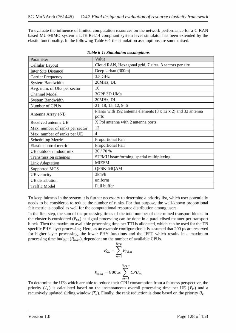
5G-MoNArch (761445) D4.2 Final design and evaluation of resource elasticity framework
Version 1.0 Page 128 of 153
To evaluate the influence of limited computation resources on the network performance for a C-RAN
based MU-MIMO system a LTE Rel.14 compliant system level simulator has been extended by the
elastic functionality. In the following Table 6-1 the simulation assumptions are summarised.
Table 6-1: Simulation assumptions
Parameter Value
Cellular Layout Cloud RAN, Hexagonal grid, 7 sites, 3 sectors per site
Inter Site Distance Deep Urban (300m)
Carrier Frequency 3.5 GHz
System Bandwidth 20MHz, DL
Avg. num. of UEs per sector 10
Channel Model 3GPP 3D UMa
System Bandwidth 20MHz, DL
Number of CPUs 21, 18, 15, 12, 9 ,6
Antenna Array eNB Planar with 192 antenna elements (8 x 12 x 2) and 32 antenna
ports
Received antenna UE X Pol antenna with 2 antenna ports
Max. number of ranks per sector 12
Max. number of ranks per UE 4
Scheduling Metric Proportional Fair
Elastic control metric Proportional Fair
UE outdoor / indoor mix 30 / 70 %
Transmission schemes SU/MU beamforming, spatial multiplexing
Link Adaptation MIESM
Supported MCS QPSK-64QAM
UE velocity 3km/h
UE distribution uniform
Traffic Model Full buffer
To keep fairness in the system it is further necessary to determine a priority list, which user potentially
needs to be considered to reduce the number of ranks. For that purpose, the well-known proportional
fair metric is applied as well for the computational resource distribution among users.
In the first step, the sum of the processing times of the total number of determined transport blocks in
the cluster is considered (𝑃𝐶𝐿) as signal processing can be done in a parallelised manner per transport
block. Then the maximum available processing time per TTI is allocated, which can be used for the TB
specific PHY layer processing. Here, as an example configuration it is assumed that 200 µs are reserved
for higher layer processing, the lower PHY functions and the IFFT which results in a maximum
processing time budget (𝑃𝑚𝑎𝑥), dependent on the number of available CPUs.
𝑃𝐶𝐿 = ∑𝑃𝑇𝐵,𝑛
𝑁𝑇𝐵
𝑛=1
𝑃𝑚𝑎𝑥 = 800µ𝑠 ∑ 𝐶𝑃𝑈𝑚
𝑁𝐶𝑃𝑈
𝑚=1
To determine the UEs which are able to reduce their CPU consumption from a fairness perspective, the
priority (𝐼𝑘 ) is calculated based on the instantaneous overall processing time per UE (𝑃𝑘 ) and a
recursively updated sliding window (𝑇𝑘). Finally, the rank reduction is done based on the priority 𝑈𝑘

5G-MoNArch (761445) D4.2 Final design and evaluation of resource elasticity framework
Version 1.0 Page 129 of 153
𝑃𝑘(𝑖) = ∑𝑃𝑛,𝑘
𝑁𝑇𝐵
𝑛=1
𝐼𝑘(𝑖) = 𝑃𝑘(𝑖)
𝑇𝑘
𝑇𝑘(𝑖 + 1) = {𝛽𝑇𝑘(𝑖) 𝑛𝑜𝑛 − 𝑠𝑐ℎ𝑒𝑑𝑢𝑙𝑒𝑑 𝑎𝑡 𝑡𝑖𝑚𝑒 𝑖
𝛽𝑇𝑘(𝑖) + (1 − 𝛽)𝑃𝑘(𝑖) 𝑠𝑐ℎ𝑒𝑑𝑢𝑙𝑒𝑑 𝑢𝑠𝑒𝑟 𝑎𝑡 𝑡𝑖𝑚𝑒 𝑖}
𝑈𝑘(𝑖) = 𝑚𝑎𝑥𝑘𝐼𝑘(𝑖)
As an example, a scheduling decision of a simplified simulation run for one sector is depicted in Figure
6-10. The sector has only one CPU available to process the scheduled TBs. 8 out of 11 active users are
scheduled in the considered TTI. As a result of the scheduling decision the processing time would be
exceeded. Therefore, based on the aforementioned elastic proportional fair metric UE 2 (second row)
suffers from the decision by taking away one rank which results in a loss of 6.9%. However, the required
processing time is not exceeded any longer and the scheduling decision can be taken as granted.
Figure 6-10: Example scheduling decision with reduced with and without elastic functionality
The lower number of available CPUs limits the total amount of bits, which can be transmitted in one
TTI. This means typically the transport block sizes are reduced and thus, the UE specific processing
time as well. Due to the CPU limitation and the nature of the proportional fair metric some users might
not be scheduled very often when the UE specific SINR is low. The priority is then increasing over time
and once the cell edge user is scheduled he gets a high amount of resources. The effect can be seen in
Figure 6-11. The CDFs show a turning point around the 75th percentile. While below the 75th percentile

5G-MoNArch (761445) D4.2 Final design and evaluation of resource elasticity framework
Version 1.0 Page 130 of 153
the UE specific processing time decreases, a higher amount of processing time is used by 25 percent of
the users.
Figure 6-11: CDFs of the UE specific processing time with limited amount of CPUs
This can be also observed in Figure 6-12 where the fairness criterion is depicted. With a reduced amount
of CPUs, the processing time distribution among the users the fairness gets worse. However, due to the
elastic proportional fair metric the fairness criterion is still fulfilled.
Figure 6-12: CDFs of the fairness criterion for the UE specific processing time distribution with
limited amount of CPUs
Next, Figure 6-12 shows the cumulated UE throughput distribution with limited number of CPUs
available compared with the reference case where infinite CPUs are assumed to not limit the
performance. It can be observed that there is only a slightly decreased user performance when the
number of CPUs are limited to 21. Due to the elastic rank control feature is can be observed that there
is a linear dependency between the limitation of CPUs and the possible performance of the system. The
reduction of ranks gives the scheduler the possibility to react on the limitation of CPUs and adapts with
the maximal possible performance to the limitation. A higher loss can be assumed for each example
when the processing of the transport blocks would be just discarded if not enough computational
resources are available. Finally, a summary of the impact on the identified KPIs, which are important in

5G-MoNArch (761445) D4.2 Final design and evaluation of resource elasticity framework
Version 1.0 Page 131 of 153
terms of the elasticity concept is given in Table 6-2: Impact on KPIs of the elastic rank control for MU-
MIMO
Figure 6-13: CDFs of the UE throughput with limited amount of resources
Table 6-2: Impact on KPIs of the elastic rank control for MU-MIMO
KPI name Meaning Impact
Minimum
footprint
Minimum resource set to provide
any output
Systems runs with limited amount of
computational resources
Reliability
Percentage of time in which a
VNF provides optimal operation
Increases the reliability of the overall system as
the radio scheduler knows how to handle on
computational resource shortages
Graceful
degradation
Perceived degradation utility vs
resource shortage
Linear degradation in average based on the
number of available CPUs
Rescuability Ability of overcoming an outage
until new resources are available
100% ability with potential dramatic reduction of
the cell capacity
Cost
efficiency
Increased number of slices to be
hosted on the same infrastructure
Potential to save computational resources if the
capacity is over dimensioned.
A number of CPUs which need to be available
dependent on the number of active users and
their radio conditions can be shared with other
functionalities

5G-MoNArch (761445) D4.2 Final design and evaluation of resource elasticity framework
Version 1.0 Page 132 of 153
7 Practical aspects of resource elasticity
In the previous chapters, we proposed a number of algorithms and solutions that bring resource elasticity
(at all levels, computational, single and cross-slice) into the network operation and included them into a
high-level architecture that extends and integrates the ones proposed in the state of the art with specific
elements that are propaedeutic to elasticity. In this chapter, instead, we provide a more pragmatic view
on network elasticity by describing some practical implication of its introduction in the network. We do
this by describing the elastic algorithms that will be implemented in the Touristic City Testbed deployed
in Turin (Section 7.1) and by describing two pieces of software that showcase i) an implementation of
a computationally elastic VNF (Section 7.2) and ii) a monitoring tool (Section 7.3) which is an enabler
of elastic network orchestration.
7.1 Elastic aspects of the Turin testbed
In this section in we describe the elasticity mechanisms that are at the basis of the “Touristic City”
testbed in Turin. The testbed will demonstrate some selected elasticity mechanisms described in this
document, with a special attention to the AI/ML aspects. The description is limited to the overall
structure of the testbed and the algorithms that are employed. A thorough evaluation of the system is
expected to be available in the final deliverable describing the testbeds.
Also, the procedures described in this section contribute to endow the network with the elasticity features
required by the use case described in Section 3.1. These mechanisms are compliant with the triggering
conditions, operational flow, and post-conditions defined in [ETSI19-ENI1], in that they entail an
improvement of the network efficiency and its capability to smoothly adapt the resource allocation and
utilisation. In a nutshell, the testbed features two different network slices: i) an eMBB slice that serves
360 videos to a virtual reality device that ii) also uses an URLLC slice to provide voice connectivity and
haptic interaction with other avatars in the scenario. From the physical infrastructure point of view, the
testbed includes a set of Physical Network Functions (PNFs) that implements the radio lower layers,
and a cloud infrastructure (composed by a larger but farther to the radio central cloud, and a closer but
less capable edge cloud)
Namely, besides the virtual reality application, the testbed will be composed by a set of functionalities
that is summarised as follows and detailed next:
• Network Slice Blueprinting and Onboarding
• VNF relocation due to latency
• Horizontal and Vertical VNF scaling (AI)
• Admission Control (AI)
Network Slice Blueprinting and Onboarding: this functionality encompasses all the baseline operation
available in a 5G MANO system. The automatic onboarding of the two network slices is a seamless
operation that allows i) tenants to define the requirements associated to each slice (in this case high
bandwidth for the eMBB and very low latency for the URLLC) and ii) the deployment of the VNF in
the cloud to fulfil the set requirements. This part has specific element of novelties for the blueprinting.
Specifically, the network slice templates that are currently being investigated by 3GPP and NGMN, and
their practical implementations with technologies such as TOSCA or OpenStack Heat are extended and
integrated with specific elasticity fields.
VNF relocation due to latency: after the first step, both network slices are orchestrated with all of their
VNFs (namely the higher layers of the RAN stack, the c-gNB) instantiated and running in the central
cloud. The MANO system continuously collects data about the network parameters of the virtual
network (i.e., latency, throughput, available and used radio resources). This is especially important for
the URLLC slice, that has very stringent requirements on the end to end latency between the UE and the
VR server running in the cloud (i.e., less then 80ms for perfect operation, less then 200ms for a not ideal
but still usable experience). For this reason, the delay is constantly monitored to avoid operational
glitches. So, in case of a sudden delay increase due to e.g., external factors such as additional network
slices coming in causing congestion in the radio and transport or internal ones like a high number of UE
connected to the VR application. In these cases, the orchestration framework triggers a relocation of the
network functions and VR application to the edge cloud, to benefit from the reduced latency.
5G-MoNArch (761445) D4.2 Final design and evaluation of resource elasticity framework
Version 1.0 Page 133 of 153
Horizontal and Vertical VNF scaling: the AI algorithm (such as the one described in Section 4.3)
running in the ENI module and the VNFM constantly monitors the cloud resources usage through
specific probes and takes orchestration decisions in case of new slices coming in. For example, when a
new eMBB slices is coming in, the intelligent orchestration framework has to take a decision about
where to run the associated VNFs and assign resources to them. Due to the scarcity of resources at the
edge, the algorithm may take one of the following decisions, based on the requirements of the incoming
eMBB slice:
• Horizontally scale the higher layer RAN stack (i.e., creating a new instantiation of the running
VNF), to support the additional load, if it is permitted
• Vertically scale the VNF if there are resources available on the same server
• Relocate the NF to a new location. In the latter case, the URLLC related functions could be kept
at the edge and just the eMBB ones are moved.
Admission Control: Throughout the network operation, the management system is constantly running
an AI/ML based algorithm, implementing selected features of the algorithms described in Section 4.2
These algorithms take as input both the available physical resources in terms of spectrum and cloud and
the current orchestration patterns. The goal is to optimise either the monetisation of the network and the
overall performance, also through periodic re-orchestrations.
7.2 Computational elasticity demonstrator
This section provides a description of the demonstrator for computational elasticity that has been
developed. The demonstrator has been developed for enabling the verification of computational
elasticity algorithms in typical mobile radio network deployments. This provides a significant means for
testing the operability of new adaptation algorithms based on machine learning strategies within the
scope of the 5G-MoNArch project and beyond.
The current status of the demonstrator addresses VNFs within the physical layer functions of an LTE
eNB since they have been identified as the most time consuming and time critical functions within the
corresponding protocol stack.
The demonstrator has been realised with the open source LTE implementation provided by Open Air
Interface [OAI]. The VNFs within the protocol stack have been extended with new functionality that
facilitates self-inspection of the VNFs in terms of computational resource utilisation and interaction with
a computational elasticity controller within the network architecture.
7.2.1 Relation to 5G-MoNArch architecture
Figure 7-1 shows how the computational elasticity demonstrator is related to the 5G-MoNArch
architecture. It comprises the network layer and the control layer and provides in the current version the
implementation of an intra-slice controller (ISC) and the corresponding northbound interface (NBI) and
southbound interface (SoBI). Further extensions regarding the handling of multiple network slices based
on a cross-slice controller (XSC) are under development.
The virtualisation infrastructure manager (VIM) is not an explicit component of the computational
elasticity demonstrator itself, but it can be emulated by corresponding configurations of the ISC, for
example in terms of computation resource utilisation restrictions and RAN performance KPIs (such as
minimum throughput or maximum latency) based on SLAs associated to specific network slices.
At the present, it is assumed the VIM specifies specific maximum computational resource utilisation
magnitudes for individual VFNs or VNF sets. The computational resource utilisation is measured in
processing time required for performing the tasks of the individual VNFs and the SLA constitutes a
configured minimum throughput that shall not be undercut. Here it has to be kept in mind that this
combination of metrics and constraint is just one possibility and that the demonstrator is in general not
restricted to this configuration.

5G-MoNArch (761445) D4.2 Final design and evaluation of resource elasticity framework
Version 1.0 Page 134 of 153
Figure 7-1: Mapping of computation elasticity demonstrator to 5G-MoNArch architecture
Following VNFs are currently evaluated per Transport Block (TB) processing in the downlink
transmission path of the physical layer:
• Transport block encoding
• Transport block scrambling
• Transport block modulation
These functions are called sequentially every TTI per transport block that is transmitted from the eNB
to a UE. In an LTE system, the TTI has the duration of 1 ms. However, it can be significantly shorter in
5G-NR in order to provide extremely low latencies at the air interface as required for 5G networks.
In order to perform the overall construction of a subframe that is transmitted within a TTI, the sum of
all involved processing times has to remain below 1 ms. Otherwise the transmission of a subframe would
have to be skipped which will yield reduced spectral efficiency or even instability of the data connection.
A typical configuration of the computational resource utilisation reporting that is performed periodically
(for example every second) by each VNF in the demonstrator is therefore the average processing time
per TTI. These reports are sent over the SoBI to the ISC where they are processed and eventually
forwarded to a control application that is attached to the NBI. Such a control application could then
enforce computational elasticity decisions in terms of VNF parameter adaptation under consideration of
specific SLAs if required, or it could inform the VIM if the amount of available computational resources
is not sufficient for fulfilling the tasks of the monitored VNFs.
7.2.2 Demonstrator setup
The overall demonstrator setup is shown in Figure 7-2. On the software side it consists of the three
entities EPC, eNB and ISC that are running on individual hosts. The hosts are established in form of
Docker containers [Doc]. The eNB with the LTE protocol stack implementation is connected the remote
radio head that is represented by a National Instruments USRP [NI]. In addition to the eNB, the
demonstrator comprises additional interference sources that can be configured and adapted in order to
emulate more realistic scenarios with statistical interference conditions in the future. It is furthermore
possible to adapt the attenuation of the downlink transmission path so that the SINR level can be adapted
on demand.

5G-MoNArch (761445) D4.2 Final design and evaluation of resource elasticity framework
Version 1.0 Page 135 of 153
Figure 7-2: Computational elasticity demonstrator setup
The control application for computational elasticity that has been developed so far within the 5G-
MoNArch project provides a graphical user interface (GUI) that is shown in Figure 7-3. It provides an
efficient tool for visualising the effectiveness and efficiency of different computational elasticity
algorithms.
In addition to the monitored downlink throughput and VNF processing time evaluation, it furthermore
shows the modulation and coding scheme (MCS) usage, the bandwidth usage, and the availability of
computational resources in terms of CPU performance.
The latter is currently modelled by the introduction of additional latencies per VNF that can be reduced
or increased during runtime of the eNB in order to emulate the relocation of specific VNFs to new hosts
with diverging performance or resource availability.
Figure 7-3: Computational elasticity controller GUI

5G-MoNArch (761445) D4.2 Final design and evaluation of resource elasticity framework
Version 1.0 Page 136 of 153
7.2.3 Experiment with fixed SINR level
This section shows an exemplary performance evaluation using the demonstrator in combination with a
basic MCS adaption algorithm for computational elasticity. The objective of the algorithm is to provide
a UE that is attached to the eNB with a specified minimum downlink throughput while at the same time
keeping the processing time required for downlink transport block encoding below a configured upper
limit. The throughput limit and the processing time limit are set to 8 Mbit/s and 158 s, respectively.
The SINR level during the evaluation is all the time above 20 dB so that the maximum MCS level (28)
can be used throughout the study. This level corresponds to 64QAM with the highest code rate supported
by LTE, considering that 256QAM is not supported by the current Open-Air Interface implementation.
The experiment comprises the following phases that are shown in Figure 7-4, Figure 7-5 and Figure 7-6:
• Phase 1: The UE is attached but there is no downlink traffic load. It can be seen that the
downlink encoding processing time is below the configured upper limit.
• Phase 2: Downlink traffic load has been activated for the attached UE. The downlink
throughput is at 17 Mbit/s and the downlink encoding processing time is at approximately
140 s, meaning that both throughput and processing time requirements are fulfilled. The
system is running stable with the maximum MCS.
• Phase 3: Now it is assumed the availability of computational resources for the encoding
function (for example in terms of CPU quota) have been reduced. One reason could for example
be that the resources are occupied by another network slice that has been activated. In the current
demonstrator setup this is emulated by adding an additional artificial latency to the encoding
function (20 s). The effect is that the processing time duration has been increased and is
actually exceeding now the defined upper limit for the encoding processing time. The increased
processing time has at that moment no impact on the throughput.
• Phase 4: At this stage the computational elasticity algorithms is activated and searches for a
suitable MCS that provide sufficient throughput while keeping the encoding processing time
below the configured limit. The algorithm is adapting the MCS but in general it could also be
applied in combination with a bandwidth adaptation. The crucial point is here that the transport
block size is reduced in order to reduce the encoding processing time.
• Phase 5: Now the algorithm has found a suitable MCS (22) that provides sufficient downlink
throughput while keeping the encoding processing time below the corresponding upper limit. If
the algorithm would not manage to fulfil both requirements, it would have to trigger the
orchestrator in order to request for example more computational resources for the downlink
channel encoding.
• Phase 6: The processing time required for the downlink encoding is now significantly reduced.
The reason could for example be the deactivation of another network slice which results in
additional availability of computational resources for the downlink encoding. As previously
described in case of Phase 3, this is emulated in the current version of the demonstrator by
significantly reducing the artificial latency that has been introduced for the processing time.
• Phase 7: The computational elasticity algorithm directly reacted and increased the MCS which
yields an increased downlink throughput. Both throughput and processing time requirements
are again satisfied, and the system is running stable the maximum MCS.
This basic example shows the suitability of the developed demonstration system for studying specific
computational elasticity algorithms in the context of network slicing. However, it has to be kept in mind
that this is just an exemplary study with an emulation of different states of computation resource
availability by means of introducing additional artificial latencies for specific network functions. More
realistic models will be addressed next.

5G-MoNArch (761445) D4.2 Final design and evaluation of resource elasticity framework
Version 1.0 Page 137 of 153
Figure 7-4: OAI experiment step 1
Phase 1:
No DL traffic load
Phase 2: Activation
of DL traffic load
Phase 3: Reduction
of available
computational
resources
Figure 7-5: OAI experiment step 2
Phase 4: Reaction
of computational
elasticity algorithm
Phase 5: Stabilised
processing time and
throughput
Figure 7-6: OAI experiment step 3
Phase 6: Reduction
of available
computational
resources and
reaction of
computational
elasticity algorithm
Phase 7: Stabilised
processing time and
throughput
7.2.4 Experiment with SINR process based on live network measurements
This section shows an exemplary performance study in which the demonstration system has been
combined with SINR measurements from a live LTE network. In order to perform studies under realistic
conditions, the SINR levels from the life network have been reproduced in the lab by means of software-
controlled power attenuators that have been integrated into the demonstrator setup.
Figure 7-7 shows the scenario with the measurement track encircling an LTE base station site consisting
of three sectors in Leipzig, Germany. Samples have been collected for approximately three minutes.
Figure 7-8 shows the distribution of the measured SINR of the scenario and the corresponding
distribution of the SINR reproduced in the demonstrator after calibration. The difference between the
distributions stem from nonlinear properties of the power attenuators used in the demonstrator setup.
Further improvements can be achieved by advanced calibration strategies that take into account these
effects.

5G-MoNArch (761445) D4.2 Final design and evaluation of resource elasticity framework
Version 1.0 Page 138 of 153
Figure 7-7: Measurement scenario
Figure 7-8: SINR calibration
Figure 7-9, Figure 7-10 and Figure 7-11 show the sample traces of downlink modulation and coding
scheme (MCS), throughput, and corresponding transport block processing that have been recorded
during a run of the demonstrator with the reproduced SINR samples. The figures show samples traces
that have been smoothed with a moving average over 1000 samples (TTIs), corresponding to a duration
of one second.
Figure 7-9: Downlink MCS trace
Figure 7-10: Downlink throughput trace
Figure 7-11: Downlink encoding processing time trace

5G-MoNArch (761445) D4.2 Final design and evaluation of resource elasticity framework
Version 1.0 Page 139 of 153
The results clearly reveal the distinct correlation between used downlink MSC, throughput and
processing time. Although this study addresses the downlink, the same assertion basically applies for
the uplink as well.
The processing time per transmission time interval 𝑇𝑝𝑖 is measured within the VNF, in the case the
downlink transport block encoding. This function is addressed in this investigation since it has been
shown that it is the most time-consuming function in the downlink transmission chain.
Since reporting of processing time samples per TTI would generate prohibitive network traffic, the VNF
furthermore provides estimations of both first moment (��1) and second moment (��2) of the processing
time population within a configured time window. The latter would for example comprise 1000 TTIs,
corresponding to one second under the assumption that each TTI has a fixed duration of one millisecond.
��𝑝1=1
𝑁𝑠∑𝑇𝑝𝑖
𝑁𝑠
𝑖=1
��𝑝2=1
𝑁𝑠∑𝑇𝑝𝑖
2
𝑁𝑠
𝑖=1
These moment estimations are sent over the SoBI to the ISC where they are processed and eventually
forwarded to a control application that is attached to the NBI. In the following it is assumed that the ICS
derives estimations for both expectation (��𝑝) and standard deviation (��𝑝) from the reported moment
estimations.
��𝑝 = ��𝑝1=1
𝑁𝑠∑𝑇𝑝𝑖
𝑁𝑠
𝑖=1
��𝑝 = √��𝑝2− ��𝑝1
2
In addition to the results, which are presented in Figure 7-12, a fixed supplementary processing time of
50 microseconds has been inflicted to the encoding every TTI. In a live network under realistic
conditions this could for examples based in reduced availability of computational resources on the
computation node that hosts the examined VNF. Besides the raw processing time samples per TTI,
Figure 7-12 furthermore contains the estimated expectation with a time window of three seconds
according to the strategy described above. A configured processing time threshold is shown as well. It
is assumed that the threshold defines an upper limit for the acceptable processing time.
The results shown in Figure 7-12 clearly show that considering only the expectation (sample mean) of
the processing time basically neglects the fact that processing time fluctuations might be quite severe,
yielding therefore frequent threshold transgressions even in cases of low processing time expectation
(samples mean). Considering both estimated expectation and standard deviation is therefore a reasonable
approach for providing accurate predictions of processing time threshold transgressions under given
radio channel and interference conditions.

5G-MoNArch (761445) D4.2 Final design and evaluation of resource elasticity framework
Version 1.0 Page 140 of 153
Figure 7-12: Downlink encoding processing time evaluation – raw samples
As described above, the ICS derives estimations for processing time expectation and processing time
standard deviation from the raw samples’ moments. These are subsequently reported to the control
application. The latter will provide decisions regarding computational elasticity or re-orchestrations.
Decisions affecting computational elasticity could for example restrict modulation and coding schemes
or transmission bandwidth in order to reduced processing time within the considered VNF.
Based on the principle of maximum entropy, an exemplary control application could for example assume
a normal distribution of the processing time with a given time window based on the reported estimations
for expectation and standard deviation. The normal distribution will provide an estimation of the
probability of crossing the configured processing time threshold.
Figure 7-13 and Figure 7-14 show examples of processing time histograms and corresponding normal
distribution estimations of two different sample subsets each comprising consecutive samples within a
time window of three seconds duration. The results show that the assumption of a normal distribution is
sufficiently accurate, especially for relevant the upper tail. The processing time threshold has been set
to 110 microseconds.
Figure 7-13: Downlink encoding processing
time evaluation – exemplary estimation A
Figure 7-14: Downlink encoding processing
time evaluation – exemplary estimation B
Based on the normal distribution assumption, consecutive sample sets (time windows) can be classified
regarding expected probabilities of threshold transgressions. Figure 7-15 shows a classification of all
three second windows of the overall run given in Figure 7-12. The distributions are marked as ‘no action
required’ and ‘action required’. The latter means that the processing time is too large and has to be
reduced, for examples by means of MCS or bandwidth restrictions. Figure 7-16 shows the time windows
that would require action corresponding to the described strategy.

5G-MoNArch (761445) D4.2 Final design and evaluation of resource elasticity framework
Version 1.0 Page 141 of 153
Figure 7-15: Downlink encoding processing
time evaluation – estimated distributions
Figure 7-16: Downlink encoding processing
time evaluation – raw samples with marked
critical regions
7.3 Monitoring tools for elastic operation
The new paradigms of 5G networks such as NFV and SDN have transformed the behaviour and
management of the networks, infrastructure and services; going from static setups, with a fixed and
stable number of physical elements inside a closed system to a changing, dynamic environment, able to
modify its shape and elements constantly, adapting to the variable demands of the network.
Managing the new flexible, elastic and self-managed networks require creating new techniques to have
the whole environment, virtual or physical, under control. Furthermore, network slicing and the
appearance of components of different nature in the architecture such as containers, requires a reviewed
monitoring solution able to provide SLA assurance and the highest possible QoS in 5G environments.
For this purpose, the below-described monitoring solution adapts to the new challenges to collect,
analyse and classify all the data necessary, from every possible source, in a dynamic way. In order to
efficiently implement the elastic mechanisms described in Chapter 4 in Touristic City Turin testbed, it
is necessary to analyse deeply the aspects that are required to provide an effective monitoring tool
adapted to the current needs of 5G-MoNArch.
Currently, the legacy monitoring systems have several limitations in terms of flexibility and adaptation
to distributed, dynamic infrastructures that change their shape and amount of resources available
according to network conditions. As an addition, they are arduous to maintain and due to their
complexity, high provisioning and operational costs are required [LOA+17].
In this section we describe a potential monitoring solution adapted to the specific requirements of the
5G-MoNarch ecosystem that is able to support the elastic mechanisms defined in this deliverable by
following these actions:
• Virtual Network Function (VNF) monitoring regarding resource usage as RAM, CPU, storage
and network in real time, to have under control the status of the different VMs that conform
each Network Service (NS).
• Take actions accordingly as horizontal or vertical scaling, by informing the orchestrator in order
to maintain the QoS during all the lifecycle of the VNFs.
• In case of latency issues caused by network bottleneck, find an optimal allocation of latency
critical VNFs between edge and central clouds, considering the trade-off between the delay and
the resource limitation.
• To support slice admission control algorithms by monitoring the virtual infrastructure.
• Validate the system design and provide outcome to the experiment-driven optimisation in a
visual way using graphs.

5G-MoNArch (761445) D4.2 Final design and evaluation of resource elasticity framework
Version 1.0 Page 142 of 153
The overall goal of monitoring in 5G-MoNArch is to provide specific metrics and rules useful to take
intelligent decisions and guarantee efficient resource usage by sending alert notifications to the different
management systems that will automate the deployment and location of VNFs and Network Slices.
The objective of this section is to evaluate the factors that are crucial to design and develop a monitoring
system to monitor every component of 5G-MoNArch at the different service and visualisation levels.
To design a flexible and reliable monitoring tool a set of rules tailored to the specific performance needs
must be defined, as well as the interfaces to send the real time alerts to the corresponding modules. Also,
the correct specification of KPIs, measured metrics, thresholds and alarms should be done to obtain a
high-performance and accurate tool. These measurements must represent and reflect the actual status of
the environment as well as provide an approach of its behaviour to predict its trends, avoiding or fixing
recognised potential issues when detected.
From a 5G-MoNarch point-of-view, the following capabilities should be addressed by the monitoring
system:
• Measure E2E slices QoS, considering the SLA to be fulfilled for each type of service,
considering and classifying their metrics and thresholds.
• Extract metrics from the components and different platforms of the system: VMs, VNFs,
containers, network and infrastructure: VIM, SDN controllers.
• Provide real-time notifications based on alerting rules. These alarms must be sent to the
orchestrator that will take decisions to mitigate the alerts.
• Perform arithmetic operations upon the collected data.
• Adapt itself to the changing conditions of the network (scalability)
• Add a dashboard that shows in a simple view the overall status of the environment
In order to efficiently measure both the virtual and physical infrastructures, a flexible, scalable and
versatile tool is required. Several studies such as [SON15-D22], and Scalable Monitoring for Multiple
Virtualised Infrastructures for 5G Services [TKL+18] have evaluated and compared multiple available
monitoring tools and have concluded that one of the most suitable tools for the 5G networks type
deployments is Prometheus [Pro]. It is an open-source, white-box monitoring and alerting toolkit. The
monitoring process consists on extracting “pull-based” metrics, making use of exporters that extract and
convert the different parameters of the service or infrastructure where the exporter is running and expose
the data as metrics in a format understandable by Prometheus. They can be installed both on the virtual
and physical machines to monitor as an executable service or as a container. There is also available a
Push Gateway to receive metrics using a “push-based” method, sent by the different services running,
but the resource consumption on Prometheus’ side limit its usage to Short-lived jobs only, with a reduced
number of metrics being sent to the gateway. The usage of exporters is the most efficient way to have a
flexible, scalable monitoring system, able to read a huge amount of metrics from multiple sources
without overload.
Prometheus allows the creation of rules, based on metrics operations with stablished limits. When the
metric value is above the limit, an alert starts firing and is sent to the alert manager that collects the
alerts, filters and aggregates them into groups, to notify about the alerts to the configured receptors
posteriorly over different channels, as an email, a REST API or a push server. Each notification contains
information about the alerts firing, including the instances, services, starting times, severities and other
custom labels included in the rules for each alert.
The definition of the KPIs that are relevant for 5G-MoNArch deployment is crucial for designing an
effective monitoring system. Some examples of KPIs and metrics that are interesting from elasticity
point of view are listed in Figure 7-17.
The KPIs are measured using metrics and arithmetic operations over them, as an average value or the
sum of several metrics over a determinate space of time, for example.
The architecture of the Prometheus ecosystem is shown in Figure 7-18. It consists of multiple
components, most of them relevant for the 5G-MoNArch monitoring tool:
The information stored by Prometheus consist of a huge number of metrics with values, timestamps and
labels, very hard to visualise and unintuitive. Grafana reads all the data from Prometheus (and other
sources) and provides tools to create, modify and manage dashboards, adding graphs, tables and

5G-MoNArch (761445) D4.2 Final design and evaluation of resource elasticity framework
Version 1.0 Page 143 of 153
percentages between others, which ease the visualisation of the environment and services performance
both in-real-time and over a specified period of time. Figure 7-19 shows the Grafana node exporter
dashboard as an example for visualising parts of the environment.
Figure 7-17: Prometheus example KPIs and metrics [Pro]
Figure 7-18: Prometheus architecture [Pro]
Figure 7-19: Grafana node exporter dashboard

5G-MoNArch (761445) D4.2 Final design and evaluation of resource elasticity framework
Version 1.0 Page 144 of 153
7.3.1 Challenges to monitoring containers
Nowadays many operators and developers decide to base their work and developments on containers,
mainly Docker [Doc] and/or Kubernetes [Kub], because of the platform independency, isolation,
resource sharing, efficiency, deployment speed, scaling options, operational simplicity, improved
development productivity and reliability from one environment to another that containers provide.
Even if containers have lots of advantages, its modularity hardens the task of monitoring the whole E2E
services, having, in some occasions, hundreds of containers being executed at the same time, running in
different nodes, with diverse metrics that have to be exported and taken into account when trying to
measure the QoS of a specific service.
As an addition, those containers can be created, scaled or destroyed frequently, making even harder to
find the different metrics data sources, which usually are fixed statically inside the monitoring systems.
It is necessary to have this dynamic environment in mind and make decisions about what and how to
monitor the QoS of services running, fully or partially, as containers. The most standardised and used
container orchestrator is Kubernetes that, in a nutshell, deploys Pods, that are the smallest basic building
blocks and are composed generally by one or more Docker containers.
In 5G-MoNArch, one container would act as a VNF while the second would be a “sidecar container”.
In order to monitor the service on a VNF basis the sidecar container would contain a customised
Prometheus exporter that monitors the VNF container. The sidecar container has preconfigured
environment variables with the VNF container id and can export the measurements to the main
Prometheus server. Each time a new service is deployed, it includes a sidecar container. Another viable
option is the usage of cAdvisor (Container Advisor), a service that communicates directly with the
Docker daemon and extracts the information from the running containers, including multiple
performance metrics in Prometheus format. One of the main advantages of cAdvisor is the fact that the
metrics are easily exposed outside the Kubernetes nodes (servers able to deploy containers using
Kubernetes), enabling the centralisation of the monitoring data in one unique Prometheus instance,
which includes rules to control the performance of the services running in containers.
7.3.2 E2E latency based on slices: difficulties measuring latency
The most efficient way to deploy E2E services is creating or modifying slices based on the needs of
each service and the availability of resources where the slice can be potentially created. Each slice has
a specific path that involves several kinds of devices and technologies (physical, virtual and RATs)
interconnected.
To measure the E2E latency of service deployed using network slices, it is essential to:
• Have the slice path well identified, including the devices involved and the kind of connections
between them to analyse, first, the set of metrics we can retrieve from them and, afterwards,
estimate the different metrics that will provide useful data about the status and performance of
the slice.
• Calculate the separated latency from the source of the service to the final device, from device
to device, measuring the response time in each step. In case the latency increases in a greater
way than expected, it is crucial to identify the origin of the problem, which could have been
generated in any of the steps previously described. The “ping” value from the source of the
service to the final device being served is not a valid metric in this case, as the only information
retrieved is the total E2E latency. It would not be possible to detect the origin of the problem
and think about a possible solution with just that information. Only if the latency between each
connection involved is correctly classified it is possible to monitor the E2E latency properly.
To empathise the importance of the previous points when measuring the point-to-point latency instead
of the total “ping”, the next example will help to clarify the concept. In the following picture, a server
is connected to three switches, that are connected to two WiFi routers and finally to the device. There is
a network slice created that connects the Server to Switch 1, Router 1 and the device respectively,
existing three different point-to-point connections to provide the E2E service. The only data provided
by the “ping” is the total E2E latency of 200 ms, but the source of this delay is generated at the
connection between the Router 1 and the device, with a latency of 180 ms and, therefore, the important
information is not collected. The information necessary to take actions to solve the problem is the

5G-MoNArch (761445) D4.2 Final design and evaluation of resource elasticity framework
Version 1.0 Page 145 of 153
connection creating the delay, not being the total latency enough to conclude to possible solutions, as
creating a new slice avoiding the Router 1.
Figure 7-20: E2E latency measurement
7.3.3 Monitoring privative/limited access VMs (unable to include exporters)
In some occasions, it is not possible to extract performance metrics from the Virtual Machines using
standard exporters, but it is imperative to have the whole infrastructure monitored to understand the
status of the whole environment and to activate actions to prevent or solve every possible problem.
Among others, the main cases where exporters cannot be installed are:
• VMs without public IP, inaccessible to the monitoring system
• VMs with privative images where nothing can be installed
• VMs with limited resources
• VMs running Operating systems incompatible with the exporters
One possible solution to have, at least, basic metric information about these Virtual Machines is to
retrieve it through the hypervisor using a LibVirt plugin that exposes basic CPU, memory, disk and
network metrics in Prometheus format, about the running instances inside the hypervisor.

5G-MoNArch (761445) D4.2 Final design and evaluation of resource elasticity framework
Version 1.0 Page 146 of 153
8 Summary and conclusions
This final public deliverable describes a consolidated view of the research developments and results
obtained within the 5G-MoNArch project in the context of resource elasticity, one of the two main
functional innovations contained in the research proposal. In particular, the document builds on the
intermediate results presented in [5GM-D41] half way through the project, highlighting primarily all
major achievements in the area reached during the second half of the project. Those include the techno-
economic analysis of elasticity, the architectural considerations in terms of components and interfaces,
and the long list of proposed elasticity mechanisms along its three dimensions, namely computational
elasticity, orchestration-driven elasticity, and slice-aware elasticity. Furthermore, this final deliverable
includes significant novelties in terms of practical aspects of elasticity demonstrated by the project,
namely the orchestration-related contributions to one of the two major project testbeds, an OAI-based
demonstrator showcasing computational elasticity and monitoring tools for elasticity.
Of particular relevance in terms of the technical output of the project in its second half is the focus on
AI and ML as a tool with immense potential to exploit elasticity in the network, hence greatly improving
resource efficiency and the overall performance of its management and orchestration machinery.
Throughout this deliverable, we have articulated the roots of its potential, the implications of making
the architecture both elastic and intelligent, and the detailed description of each elasticity mechanism
utilising this tool.
In the rest of this chapter, we provide a summarised description of the different technical contributions
contained in this deliverable sorted by chapters, highlighting both the most important results as well as
the relevant dissemination and standardisation activities carried out to increase the impact of the results
to the wider community.
• Chapter 2 has presented a techno-economic analysis of elasticity that has served as motivation
for the ensuing research work; in particular, a techno-economic analysis has revealed the impact
of elasticity on network cost savings as described both by introducing the feature in network
equipment and making the deployment of temporary hotspot more commercially attractive.
Indeed, a new case study on elasticity has been presented addressing the commercial feasibility
of temporary hotspots in MNO-driven deployments and emerging deployment models. Results
stemming from this study were disseminated at the EuCNC conference and the
Telecommunications Policy journal by Elsevier.
• Chapter 3 has introduced the building blocks of an intelligent and elastic architecture. We
have provided the full description of the elastic architecture, complementing the overall
architecture defined by the project in other work packages with the specification of all relevant
interfaces and high-level procedures for the elastic operation of the network and their
components. MSCs have been introduced for elastic network operations along the three above
mentioned dimensions of elasticity. In addition, each dimension of elasticity has been mapped
to the overall architecture in terms its relevant components. Hence, by introducing AI and
analytics as a built-in feature in the network architecture enabling elasticity, we have effectively
proposed an elastic and intelligent architecture. More specifically, we have provided an
extension of the ETSI ENI architecture, a piece of work currently ongoing within this ISG. The
rationale behind this choice has been two-fold. First, the ETSI ENI architecture is, in turn,
relying on the ETSI NFV architecture. As 5G-MoNArch is fully considering ETSI NFV as
baseline for the MANO architecture, the alignment of this architecture with the project one will
be seamless. The second one relates to the topic itself: many of the solutions and algorithms
captured in this deliverable are actually relying on AI, making them very suitable for this kind
of approach. The research carried out in this area has been particularly fruitful: first, a paper
with our overarching vision of an intelligent and elastic architecture has been accepted for
publication at the high impact factor journal IEEE Wireless Communications Magazine;
furthermore, a very fruitful collaboration has been established with ETSI ENI, where a new use
case on AI-based elastic management and orchestration has been approved, resulting in five
contributions to the SDO as well as the approval of a new proof-of-concept within ENI based
on 5G-MoNArch’s testbed on elasticity. In addition, a workshop co-organised with ETSI ENI
and the 5GPPP project SliceNet on AI for networks featuring this work has been approved for

5G-MoNArch (761445) D4.2 Final design and evaluation of resource elasticity framework
Version 1.0 Page 147 of 153
the 2019 edition of EuCNC. Several invited talks on this topic have also been (or will be)
delivered at different venues and universities, namely the Italian Networking Workshop 2019,
University of Pavia, University of Lorraine, and the Lipari Summer School of 2019.
• Chapters 4, 5 and 6 have presented the full list and description of elasticity mechanisms
developed within the project, summarised in Table 1-1, spanning all three dimensions of
elasticity: Chapter 4 has provided a number of novel contributions that demonstrate how new
elastic AI/ML-based algorithms improve the elastic network lifecycle management
performance; Chapter 5 has described the advantages of elastic resource management and
provide detailed algorithms that achieve this goal, using different approaches such as advanced
optimisation techniques or game theory; Chapter 6 has been devoted to the elastic design of
VNFs that can gracefully scale when the available cloud resources are temporally not enough.
It has been shown how by using resource-elastic network functions the elastic resource
management algorithm (both AI-based and not) can also improve resource utilisation. In
addition, a comprehensive set of evaluation results for every mechanism has been provided
along with a novel analysis on its impact on the relevant KPIs for elasticity defined in [5GM-
D41]. The rich results of these research activities have been published in a number of high-
visibility venues such as IEEE Transactions on Wireless Communications, IEEE Transactions
on Mobile Computing, ACM Mobicom, IEEE Infocom, or IEEE ICC.
• Chapter 7 has presented practical implementation aspects of elasticity with a particular focus
on two initiatives: first, the elasticity innovations being implemented in the 5G-MoNArch
Touristic City Testbed are described as some of the techniques and solutions described in this
document will be showcased in that framework, providing a view on how elasticity can improve
the network operation with a real-world service; second, we have also developed an
experimental lab demonstration based on OAI on elasticity at VNF level, (i.e., computational
elasticity) whose insights further corroborate the advantages of resource elasticity in setup closer
to reality; third, monitoring tools required for elasticity have also been described. These results
will be showcased live at the two final public dissemination events in Turin and Hamburg.
Finally, the main take-away message of this comprehensive research effort is our vision that resource
elasticity will play a very central role in the management, orchestration and control of 5G networks,
where elastic architectural components, executing elastic mechanisms aided by AI and data analytics,
will be able to extraordinarily boost the cost-efficiency of future 5G infrastructure deployments.

5G-MoNArch (761445) D4.2 Final design and evaluation of resource elasticity framework
Version 1.0 Page 148 of 153
References
[3GPP15-36213] 3GPP TS 36.213,” Evolved Universal Terrestrial Radio Access (E-UTRA);
Physical layer procedures,” v12.5.0, Rel. 12, Mar. 2015
[3GPP17-38801] 3GPP TR38.801, “Study on new radio access technology: Radio access
architecture and interfaces,” v14.0.0, March 2017
[3GPP18-23501] 3GPP TS23.501 “System Architecture for the 5G System; Stage 2, Release
15,” Dec. 2018
[3GPP18-28530] 3GPP TS 28.530, “Management and orchestration; Concepts, use cases and
requirements,” v2.0.0, June 2018
[3GPP18-28531] 3GPP TS 28.531, “Management and Orchestration – Provisioning,” v15.0.0,
Dec. 2018
[3GPP18-28801] 3GPP TR 28.801, “Study on management and orchestration of network
slicing for next generation network,” Jan. 2018
[3GPP18-38305] 3GPP TS 38.305, “NG Radio Access Network (NG-RAN); Stage 2
functional specification of User Equipment (UE) positioning in NG-RAN
(Release 15),” v15.0.0, June 2018
[3GPP19-38401] 3GPP TS 38.401, “NG Radio Access Network (NG-RAN); Architecture
description (Release 15),” v15.4.0, Jan. 2019
[5GM-D22] 5G-MoNArch Deliverable D2.2, “Initial overall architecture and concepts for
enabling innovations,” June 2018.
[5GM-D41] 5G-MoNArch Deliverable 4.1, “Architecture and mechanisms for resource
elasticity provisioning,” May 2018.
[5GM-D51] 5G-MoNArch Deliverable D5.1, “Testbed setup and 5G-MoNArch
technologies demonstrated,” August 2018.
[5GM-D62] 5G-MoNArch Deliverable D6.2, “Methodology for verification and
validation of 5G-MoNArch architectural innovations,” July 2018.
[5GN-D23] 5G NORMA Deliverable D2.3, “Evaluation of architecture design and socio-
economic analysis – final report,” December 2017.
[5GM-w] 5G-MoNArch website: https://5g-monarch.eu/ [Accessed March 2019].
[5GPPP17] 5th Generation Public Private Partnership (5G-PPP) Architecture Working
Group, “View on 5G Architecture,” White Paper, version 2.0, 2017
[ALE+17] A. Awada, A. Lobinger, A. Enqvist, A. Talukdar and I. Viering, “A
simplified deterministic channel model for user mobility investigations in 5G
networks,”2017 IEEE International Conference on Communications (ICC),
Paris, 2017, pp. 1-7.
[ANT17] O. Arouk, N. Nikaein, and T. Turletti, “Multi-objective placement of virtual
network function chains in 5G,” in 2017 IEEE 6th International Conference
on Cloud Networking, September 2017, pp. 1–6.
[ATN+18] O. Arouk, T. Turletti, N. Nikaein, and K. Obraczka, “Cost Optimisation of
Cloud-RAN Planning and Provisioning for 5G Networks,” in IEEE
International Conference on Communications, May 2018.
[ATX15] Ioannis Angelopoulos, Eleni Trouva, George Xilouris “A monitoring
framework for 5G service deployments,” 2017
[AWC18] A. Alabbasi, X. Wang, and C. Cavdar, “Optimal Processing Allocation to
Minimise Energy and Bandwidth Consumption in Hybrid CRAN,” IEEE
Transactions on Green Communications and Networking, vol. 2, no. 2, pp.
545–555, June 2018.
[AWS18] Amazon Web Services, “Amazon ec2 pricing,” [Online], Available:
https://aws.amazon.com/ec2/pricing/on-demand/ =0pt, 2018.
[B+05] E. K. Burke, et al., Search Methodologies. Springer, 2005.

5G-MoNArch (761445) D4.2 Final design and evaluation of resource elasticity framework
Version 1.0 Page 149 of 153
[BAG+18] D. Bega, A. Banchs, M. Gramaglia, X. Costa-Pérez and P. Rost, “CARES:
Computation-aware Scheduling in Virtualised Radio Access Networks,”
in IEEE Transactions on Wireless Communications, 2018.
[BGB+17] Dario Bega, Marco Gramaglia, Albert Banchs, Vincenzo Sciancalepore,
Konstantinos Samdanis, Xavier Costa-Perez, “Optimising 5G infrastructure
markets: The business of network slicing” in Proc of IEEE INFOCOM 2017-
IEEE Conference on Computer Communications.
[BHS97] T. Back, U. Hammel, and H.-P. Schwefel, “Evolutionary computation:
comments on the history and current state,” IEEE Trans. Evol. Comput., vol.
1, no. 1, pp. 3–17, Apr. 1997.
[BIY10] Biscani, F., Izzo, D., & Yam, C. H., “A Global Optimisation Toolbox for
Massively Parallel Engineering Optimisation,” 4th International Conference
on Astrodynamics Tools and Techniques (ICATT 2010), 2010
[BJD+14] E. Björnson, E. A. Jorswieck, M. Debbah, and B. Ottersten, “Multiobjective
signal processing optimisation: The way to balance conflicting metrics in 5G
systems,” IEEE Signal Process. Mag., vol. 31, no. 6, pp. 14–23, 2014.
[BPL18] M. Baghani, S. Parsaeefard, and T. Le-Ngoc, “Multi-Objective Resource
Allocation in Density Aware Designed of C-RAN in 5G,” IEEE Access, vol.
PP, no. c, pp. 1–1, 2018.
[BRH+18] F. Bahlke, O. D. Ramos-Cantor, S. Henneberger, and M. Pesavento,
“Optimised cell planning for network slicing in heterogeneous wireless
communication networks,” IEEE Commun. Lett., vol. 22, no. 8, pp. 1676–
1679, 2018.
[CBV+17] P. Caballero, A. Banchs, G. de Veciana, and X. Costa-Perez, “Network
Slicing Games: Enabling Customisation in Multi-Tenant Networks,” in
Proc. of IEEE INFOCOM, May 2017.
[Cis17] Cisco, “Cisco Visual Networking Index: Forecast and Trends, 2016-2021,”
June 2017.
[CSR+15] E. F. Coutinho et al., “Elasticity in cloud computing: A survey,” Annals of
Telecommunications, vol. 70, no. 7-8, Aug. 2015.
[CZA+17] J. Cao, Y. Zhang, W. An, X. Chen, J. Sun, and Y. Han, “VNF-FG design and
VNF placement for 5G mobile networks,” Sci. China Inf. Sci., vol. 60, no. 4,
2017.
[CZW+18] Chen, X., Zhang, H., Wu, C., Mao, S., Ji, Y. and Bennis, M., “Optimised
computation offloading performance in virtual edge computing systems via
deep reinforcement learning,” in IEEE Internet of Things Journal 2018 Oct.
2018.
[DGB+12] H. S. Dhillon, R. K. Ganti, F. Baccelli, and J. G. Andrews, “Modeling and
Analysis of K-Tier Downlink Heterogeneous Cellular Networks,” IEEE
Journal on Selected Areas in Communications, vol. 30, no. 3, pp.550–560,
2012
[DLY19] A. De Domenico, Y.-F. Liu, and W. Yu, “Optimal Virtual Network Function
Deployment for 5G Network Slicing in Hybrid Cloud Infrastructure,” in
IEEE ICASSP 2019, to be published.
[Doc] Docker Inc [n.d.], Future proof your Windows apps and drive continuous
innovation, [Online] available: https://www.docker.com/ [Accessed January
2019]
[DSM+18] M. Dighriri, A. Saeed Dayem Alfoudi, G. Myoung Lee, T. Baker, and R.
Pereira, “Resource Allocation Scheme in 5G Network Slices,” 2018 32nd
International Conference on Adv. Inf. Netw. Appl. Work., pp. 275–280,
2018.
[ENI17] ETSI ENI, “Improved operator experience through Experiential Network
Intelligence,” White Paper, Oct. 2017.

5G-MoNArch (761445) D4.2 Final design and evaluation of resource elasticity framework
Version 1.0 Page 150 of 153
[ETSI16-NFV] ETSI NFV, “GS NFV-REL 004 Network Functions Virtualisation (NFV);
Assurance; Report on Active Monitoring and Failure Detection,” v1.1.1,
April 2016
[ETSI17-012] ETSI GR NFV-EVE 012, v3.1.1, “Network functions virtualisation (NFV)
release 3; Evolution and ecosystem; Report on network slicing support with
ETSI NFV architecture framework,” Dec. 2017.
[ETSI19-ENI1] ETSI RGS ENI 008 (GS ENI 001), “Experiential Networked Intelligence
(ENI); ENI Use Cases,” v.2.0.4 (under development, expected publication in
2019), Sec 5.3.6
[FGY+17] M. J. Farooq, H. Ghazzai, E. Yaacoub, A. Kadri, and M.-S. Alouini, “Green
Virtualisation for Multiple Collaborative Cellular Operators,” IEEE Trans.
Cogn. Commun. Netw., vol. 3, no. 3, pp. 420–434, Sep. 2017.
[FJ08] J. Fulcher and L. C. Jain (Eds.), “Computational Intelligence: A
Compendium,” vol. 115. Berlin, Heidelberg: Springer Berlin Heidelberg,
2008.
[FMK17] X. Foukas, M. K. Marina, and K. Kontovasilis, “Orion: RAN Slicing for a
Flexible and Cost-Effective Multi-Service Mobile Network Architecture,” In
Proceedings of the 23rd Annual International Conference on Mobile
Computing and Networking (ACM MobiCom), 2017.
[GPD+18] D. M. Gutierrez-Estevez, N. di Pietro, A. De Domenico, M. Gramaglia, U.
Elzur, and Y. Wang, “5G-MoNArch use case for ETSI ENI: elastic resource
management and orchestration,” in Proc. IEEE CSCN, Paris, France, 2018.
[GF15] I. Giagkiozis and P. J. Fleming, “Methods for multi-objective optimisation:
An analysis,” Inf. Sci. (Ny)., vol. 293, pp. 338–350, Feb. 2015.
[GJ79] Michael R. Garey, David S. Johnson, “Computers and Intractability: A Guide
to the Theory of NP-Completenes,” W. H. Freeman & Co. New York, NY,
USA ©1979, ISBN 0716710447.
[GLK14] A. Gudipati, L. E. Li, and S. Katti, “RadioVisor: A Slicing Plane for Radio
Access Networks,” in Proc. of HotSDN, 2014.
[HKR13] N. R. Herbst, S. Kounev, and R. H. Reussner, “Elasticity in Cloud
Computing: What It Is, and What It Is Not,” In Proc. International
Conference on Autonomic Computing (ICAC), vol. 13, pp. 23-27, Jun. 2013.
[HLS18] B. Han, J. Lianghai, and H. D. Schotten, “Slice as an Evolutionary Service:
Genetic Optimisation for Inter-Slice Resource Management in 5G
Networks,” IEEE Access, vol. 6, pp. 33137–33147, 2018.
[HS16] M. Hausknecht and P. Stone, “Deep reinforcement learning in parameterised
action space,” International Conference on Learning Representations (ICLR),
2016.
[HSW89] K. Hornik, M. Stinchcombe, and H. White, “Multilayer feedforward
networks are universal approximators,” Neural networks, vol. 2, no. 5, pp.
359–366, 1989.
[ITU09-M21351] ITU-R M.2135-1, “Guidelines for evaluation of radio interface technologies
for IMT-Advanced,” Technical Report, Dec 2009.
[Jac01] P. Jaccard, “Etude comparative de la distribution florale dans une portion des
alpes et des jura,” Bull Soc Vaudoise Sci Nat, vol. 37, pp. 547–579, 1901.
[Jai10] A. K. Jain, “Data clustering: 50 years beyond k-means,” Pattern Recognition
Letters, vol. 31, no. 8, pp. 51–666, 2010.
[KAL+18] U. Karabulut, A. Awada, A. Lobinger, I. Viering, M. Simsek and G. P.
Fettweis, “Average downlink SINR model for 5G mmWave networks with
analog beamforming,” 2018 IEEE Wireless Communications and
Networking Conference (WCNC), Barcelona, 2018, pp. 1-6.
[KC14] S. Khatibi, L.M. Correia, “Modelling of Virtual Radio Resource
Management for Cellular Heterogeneous Access Networks,” in Proc.

5G-MoNArch (761445) D4.2 Final design and evaluation of resource elasticity framework
Version 1.0 Page 151 of 153
PIMRC’14 – IEEE 25th International Symposium on Personal, Indoor and
Mobile Radio Communications, Washington, USA, Sep. 2014.
[KDT14] I. Kalamaras, A. Drosou, and D. Tzovaras, “Multi-objective optimisation for
multimodal visualisation,” IEEE Trans. Multimed., vol. 16, no. 5, pp. 1460–
1472, 2014.
[Ker] Keras Documentation [n.d.], “Keras: The Python Deep Learning Library,”
[Online] available at http://keras.io/
[KN17] A. Ksentini and N. Nikaein, “Toward Enforcing Network Slicing on RAN:
Flexibility and Resources Abstraction,” IEEE Communications Magazine no.
55, 6, June 2017.
[Kou17] I. Koutsopoulos, “Optimal functional split selection and scheduling policies
in 5G Radio Access Networks,” in IEEE International Conference on
Communications Workshops, May 2017, pp. 993–998.
[KQ98] A. F. Kuri-Morales and C. C. Quezada, “A universal eclectic genetic
algorithm for constrained optimisation,” Proc. 6th Eur. Congr. Intell. Tech.
Soft Comput. EUFIT’98, pp. 2–6, 1998.
[KSR18] Khatibi, S., Shah, K., & Roshdi, M., “Modelling of Computational Resources
for 5G RAN,” In EuCNC’18 - IEEE European Conference on Networks and
Communications (pp. 1–5), Jun. 2018.
[Kub] Kubernetes [n.d.], “Production-Grade Container Orchestration”, [Online]
available: https://kubernetes.io/
[LOA+17] M. Liyanage, J. Okwuibe, I. Ahmed, M. Ylianttila, O. López Pérez, M.
Uriarte Itzazelaia, E. Montes de Oca, “Software Defined Monitoring (SDM)
for 5G mobile backhaul networks,” July 2017
[LSO+14] L. A. Lopes, R. Sofia, H. Osman and H. Haci, “A proposal for elastic
spectrum management in wireless local area networks,” 2014 IEEE
Conference on Computer Communications Workshops (INFOCOM
WKSHPS), Toronto, ON, 2014, pp. 127-128
[Lux07] U. Von Luxburg, “A tutorial on spectral clustering,” Statistics and
computing, vol. 17, no. 4, pp. 395–416, 2007.
[LZG+15] J. Liu, S. Zhou, J. Gong, Z. Niu, and S. Xu, “Graphbased framework for
flexible baseband function splitting and placement in C-RAN,” in IEEE
International Conference on Communications (ICC), June 2015, pp. 1958–
1963.
[MB12] Kevin P. Murphy, Francis Bach, “Machine learning: a probabilistic
perspective,” MIT Press, 2012.
[MBC+16] F. Musumeci, C. Bellanzon, N. Carapellese, M. Tornatore, A. Pattavina, and
S. Gosselin, “Optimal BBU Placement for 5G C-RAN Deployment Over
WDM Aggregation Networks,” Journal of Lightwave Technology, vol. 34,
no. 8, pp. 1963–1970, April 2016.
[MG79] R. Michael, S. Garey David, “Johnson Computers and Intractability: A Guide
to the Theory of NP-Completenes,” W. H. Freeman & Co. New York, NY,
USA 1979, ISBN 0716710447.
[MGF+18] C. Marquez, M. Gramaglia, M. Fiore, A. Banchs, and X. Costa-Perez, “How
Should I Slice My Network? A Multi-Service Empirical Evaluation of
Resource Sharing Efficiency,” In The 24th Annual International Conference
on Mobile Computing and Networking (MobiCom ’18).
[MGL04] V. Maniezzo, L. Gambardella, and F. de Luigi, “Ant Colony Optimisation,”
in New Optimisation Techniques in Engineering, Springer Berlin Heidelberg,
vol. 141, pp. 101-121, 2004.
[MW00] J. Mo and J. Walrand, “Fair end-to-end window-based congestion control,”
IEEE/ACM Transactions on Networking, vol. 8, no. 5, pp. 556--567, Oct.
2000.

5G-MoNArch (761445) D4.2 Final design and evaluation of resource elasticity framework
Version 1.0 Page 152 of 153
[NGMN15] Next Generation Mobile Networks (NGMN) Alliance, “5G WhitePaper,”
Feb. 2015.
[NI] National Instruments, [n.d.], website, http://www.ni.com/
[NJW02] A. Y. Ng, M. I. Jordan, and Y. Weiss, “On spectral clustering: Analysis and
an algorithm,” in Advances in neural information processing systems, 2002,
pp. 849–856.N
[OAI] Eurecome Open Air Interface, [n.d.]. “OpenAirInterface: 5G software
alliance for democratising wireless innovation,” [Online] available at
https://www.openairinterface.org/
[PDD+17] S. Parsaeefard, R. Dawadi, M. Derakhshani, T. Le-Ngoc, and M. Baghani,
“Dynamic Resource Allocation for Virtualised Wireless Networks in
Massive-MIMO-Aided and Fronthaul-Limited C-RAN,” IEEE Transactions
on Vehicular Technology., vol. 66, no. 10, pp. 9512–9520, 2017.
[Pro] Prometheus [n.d.], “From metrics to insight,” [Online] available at
https://prometheus.io
[RAH+18] Rahman, S., Ahmed, T., Huynh, M., Tornatore, M. and Mukherjee, B.,
“Auto-scaling network resources using machine learning to improve QoS and
reduce cost,” arXiv preprint:1808.02975, 2018.
[RTN97] R. Ramjee, D. Towsley, and R. Nagarajan, “On Optimal Call Admission
Control in Cellular Networks,” Wireless Networks, vol. 3, no. 1, pp. 29--41,
Mar. 1997.
[S+17] Silver, David, et al., “Mastering the game of Go without human
knowledge,” Nature, 550.7676 (2017): 354.
[SA13] N. Siddique and H. Adeli, “Computational Intelligence: Synergies of Fuzzy
Logic, Neural Networks and Evolutionary Computing,” Wiley, 2013.
[SCC17] V. Sciancalepore, F. Cirillo, and X. Costa-Perez, “Slice as a Service (SlaaS)
Optimal IoT Slice Resources Orchestration,” in GLOBECOM 2017 - 2017
IEEE Global Communications Conference, 2017, pp. 1–7.
[Sch07] S.E. Schaeffer, “Graph clustering,” Computer Science Review, Volume 1,
Issue 1, 2007, Pages 27-64.
[SCS16] K. Samdanis, X. Costa-Perez, and V. Sciancalepore, “From network sharing
to multi-tenancy: The 5G network slice broker,” IEEE Communications
Magazine vol 54, no. 7, July 2016, pp 32–39.
[SLH+14] Silver, D., Lever, G., Heess, N., Degris, T., Wierstra, D. and Riedmiller, M.,
“Deterministic policy gradient algorithms,” in proc. ICML, 2014.
[SON15-D22] SONATA Deliverable D2.2, “Architecture Design,” December 2015.
[TCS+15] C.-W. Tsai, H.-H. Cho, T. K. Shih, J.-S. Pan, and J. J. P. C. Rodrigues,
“Metaheuristics for the deployment of 5G,” IEEE Wirel. Commun., vol. 22,
no. 6, pp. 40–46, Dec. 2015.
[Tib96] Tibshirani, R., “Regression Shrinkage and Selection via the Lasso,” Journal
of the Royal Statistical Society. Series B, Vol. 58, No. 1, 1996, pp. 267–288.
[TKL+18] P. Trakadas, P. Karkazis, H-C Leligou, T. Zahariadis, W.Tavernier, T.
Soenen, S. V. Rossem, L. M. Contreras Murillo, “Scalable Monitoring for
Multiple Virtualized Infrastructures for 5G Services,” The International
Symposium on Advances in Software Defined Networking and Network
Functions Virtualization (SoftNetworking), 2018
[VGL04] V. Maniezzo, L. Gambardella, and F. de Luigi, “Ant Colony Optimisation,”
in New Optimisation Techniques in Engineering, Springer Berlin Heidelberg,
vol. 141, pp. 101-121, 2004.
[WFC+18] Y. Wang, R. Forbes, C. Cavigioli, H. Wang, A. Gamelas, A. Wade, J.
Strassner, S. Cai, S. Liu, “Network Management and Orchestration using

5G-MoNArch (761445) D4.2 Final design and evaluation of resource elasticity framework
Version 1.0 Page 153 of 153
Artificial Intelligence: Overview of ETSI ENI,” IEEE Communications
Standards Magazine 2, no. 4, Dec. 2018.
[WFT+18] G. Wang, G. Feng, W. Tan, S. Qin, R. Wen, and S. Sun, “Resource
Allocation for Network Slices in 5G with Network Resource Pricing,” 2017
IEEE Glob. Commun. Conf. GLOBECOM 2017 - Proc., vol. 2018–Janua,
pp. 1–6, 2018.
[XLY18] S. Xu, R. Li, and Q. Yang, “Improved genetic algorithm based intelligent
resource allocation in 5G Ultra Dense networks,” IEEE Wireless
Communication Networks Conf. WCNC, vol. 2018–April, pp. 1–6, 2018.
[ZL07] Q. Zhang and H. Li, “MOEA/D: A Multiobjective Evolutionary Algorithm
Based on Decomposition,” IEEE Trans. Evol. Comput., vol. 11, no. 6, pp.
712–731, 2007.
[ZLC+17] H. Zhang, N. Liu, X. Chu, K. Long, A. H. Aghvami, and V. C. M. Leung,
“Network Slicing Based 5G and Future Mobile Networks: Mobility,
Resource Management, and Challenges,” IEEE Commun. Mag., vol. 55, no.
8, pp. 138–145, 2017.
[ZPH18] C. Zhang, P. Patras, H. Haddadi, “Deep Learning in Mobile and Wireless
Networking: A Survey,” arXiv pre-print: 1803.04311, 2018.