5.4 project finance models, analytical techniques for
TRANSCRIPT

Section 5 – Framework for Financing Merchant Power Plants Page 5-1 of 89
5.4 Project Finance Models, Analytical Techniques for Evaluating MPPs
This section describes analytical models that can be used to underwrite loans and determine the
credit spread for merchant power plant transactions from the perspective of the ADB. There are
two general types of models used to evaluate MPP risks -- project finance models and forward
price simulation models:
1) Project finance models measure value and credit risk from an investor perspective --
including debt investors, equity investors and investment by multilateral agencies
such as the ADB.
2) Forward price simulation models measure future electricity prices, price volatility and
the impacts of alternative market frameworks on customers and investors. The price
forecasts in these models are inputs to project finance models of merchant power
plants. Forward price simulation models also can be used to quantify impacts of
policy issues through measuring total cost to customers, prices faced by customers,
incentives for developers to make investments, system reliability, price volatility and
other factors. These subjects are addressed in section 5.7.
The remainder of this section describes how project finance models and forward price simulation
models can be used to quantify risks of merchant power plants. Application of the project finance
models to MPPs includes use of models to determine break-even prices and sensitivity; definition
and measurement of electricity price volatility; use of Monte Carlo simulation in measuring risks
associated with merchant power plants. The discussion of forward price simulation models
considers long-run marginal cost analysis and complex simulation analysis that incorporates the
behaviour of MPP developers.
5.4.1 Project Finance Models
A basic tool for risk analysis of merchant plants is a model of how cash flows are
affected by market risk. Project finance models used in measuring risks associated
with merchant power plants below have equations for optimizing debt capacity,
measuring chances of going bankrupt, and calculating the electricity price that would
be required in bilateral contracts (the software is included on the attached compact
disk). Outputs from a project finance model include the internal rate of return on the
equity investment and the internal rate of return on aggregate project free cash flow,
debt service coverage ratios and the amount of debt that cannot be re-paid at the
end of the life of a project.
The following statement made by Fitch Investor Services describes how project
finance models are the centrepiece of assessing the credit quality of merchant power
plants:
Models of projected cash flow are a very significant component in the
credit evaluation of merchant plant transactions. In a merchant power
project, cash flow forecasting is based on a model [that is] a
reasonably accurate representation of the project’s expected operating
performance and operating expenses at varying levels of output over
the life of the debt. The model also incorporates the terms of the
financial structure, debt amortization, and interest payments… Fitch
reviews the base case and various stress scenarios affecting project
cash flows. Typical cases include lower market prices than the base

Section 5 – Framework for Financing Merchant Power Plants Page 5-2 of 89
case, higher operating costs, lower gas prices, unscheduled outages,
or changes in environmental regulation.
Project finance models have long been used by the ADB and others to evaluate
many investments including electricity plants with long-term purchase contracts. The
project finance models used in evaluating merchant power risk must be able to
measure the effects of price volatility; merchant plant debt enhancements such as
cash flow sweeps and cash flow traps; debt service reserves; risk mitigation from
bilateral contracts; subordinated debt structures; risk absorption by fuel suppliers and
other characteristics associated with merchant plants.
To illustrate how project finance models are used in the context of evaluating a
merchant plant and how this contrasts from plants with long-term PPA contracts we
summarize selected issues discussed later on in the report. The table below shows
how a cash flow trap covenant, a cash flow sweep covenant, alternative leverage,
and a bilateral contract can moderate the risks associated with a merchant plant. A
full description of these issues sweeps in the context of ADB’s underwriting process
for the debt of an MPP is described in Sections 5.5 and 5.6. We summarise the
analysis here to show the unique way in which project finance models are used
together with price volatility, simulation and credit analysis in the underwriting of MPP
transactions. The table below demonstrates the financial structure of an MPP can
have an important effect on the probability of default that the plant will not be able to
pay off debt and the required pricing of MPP debt issued by the ADB or other lenders.
In a case without structural enhancements -- cash sweeps, cash traps and a debt
service reserve -- the probability of default for the NGCC plant is 4.67% assuming
electricity price volatility of 25% and 14.64% assuming a very high price volatility of
14.74%. If a cash flow trap and cash flow sweep covenants are included in the
transaction tied to the debt service coverage ratio, the credit spread falls to 2.93%. If
a bilateral contract is used to mitigate risks associated with price volatility, the
required pricing falls to 2.19%. The process for measuring MPP risks and structuring
MPP debt to mitigate the risks is explained in the remainder of the report.
The table illustrates the type of analysis that is required for assessing the risk of an
MPP – volatility and trends in electricity prices must be established; probability of loss
and loss, given default should be assessed; alternative structural enhancements

Section 5 – Framework for Financing Merchant Power Plants Page 5-3 of 89
should be measured; debt service reserves must be taken into account. The risks
can then be translated into DSCR benchmarks and debt leverage ratio benchmarks
for different types of plants.
5.4.2 Break-even Analysis, Scenario Analysis and Sensitivity Analysis
The next sections describe project finance models can be applied in assessing the
risk of a merchant power plant. This section discusses traditional approaches to
assess risk that are derived from using expert judgement on economic variables such
as the electricity price. The next section introduces mathematical techniques that
incorporate the price volatility of electricity and apply Monte Carlo simulation to
project finance models.
Traditional methods of using a project finance model with expert judgement to assess
the risk of an MPP include break-even analysis, scenario analysis and sensitivity
analysis:
Sensitivity analysis evaluates how the credit quality and value of an MPP is
affected by changing single variables.
Scenario analysis measures the ability of an MPP to service debt and generate
cash flow under a set of assumptions for market prices, fuel costs, plant
availability and other variables.
Break-even analysis tests how much worse a variable can become before a
default or non-payment of debt occurs. Break-even analysis can be applied to
the minimum debt service coverage ratio or the amount of debt outstanding at
the end of the life of a project.
The following quotes from bond rating agencies Fitch and Moody’s illustrate how the
use of sensitivity analysis, scenario analysis and break-even analysis is applied in the
underwriting of merchant power plant transactions:
Fitch
The object is to determine if the project is likely to continue to cover operating
expenses and debt interest and principal payments despite unexpected
stress levels. The scenarios also reveal whether there are particular
variables to which the project has a greater degree of sensitivity. The
evaluation of the stress scenario results is focused on the minimum debt
service coverage in any single year and the average debt service coverage
over the entire life of the debt. If the cash flows are unable to cover payments
on project debt under certain stress scenarios, the debt service reserve or
other forms of credit enhancement available to the project are applied. Thus,
[sensitivity analysis] can be used to size the appropriate debt service reserve
or other credit enhancements needed to avoid default under adverse
scenarios. Fitch performs sensitivity analyses that stress cash flows down to
a break-even level to see how the project performs under extreme hardship
conditions and at what minimum power price the project can perform while
covering operating costs and debt service payments.
Moody’s
Section 5 – Framework for Financing Merchant Power Plants Page 5-4 of 89
Moody’s believes that the appropriate analytical beginning is to determine a
credible market forecast and to assess the projects break-even position
relative to that market forecast. A break-even point substantially below the
market forecast allows a project to absorb unexpected market fluctuations in
prices and volumes which is essential to an investment grade debt security.
From this analysis, one can derive the appropriate capital structure for each
project individually.
Moody’s believes that a merchant plant will be subject to swings in prices as
power markets develop. The better able a project is to absorb changes in
prices (and changes in volumes) the higher its rating will be. Our belief is
that an investment-grade-rated merchant power plant will have a break-even
point, where it fully covers its debt service obligations, between 30% and
50% below a reasonable market forecast price. The amount of the
discount is determined by the characteristics of the market and the
reasonableness of the market forecast assumptions.
Standard & Poor's
Where projects elect to obtain key supply inputs from spot markets, the risk
of cash flow erosion may raise project credit concerns, particularly in volatile
markets, such as energy and other commodities. Stronger projects will be
those that can demonstrate a resilience to worst case cost movement
scenarios as indicated by historical trends. Historical price trends in such
commodities as crude oil, petrochemical products, metals and pulp and
paper can provide a basis for analysis of potential worst case price
movements. Standard & Poor's will rely in part on financial scenario analysis
to assess the effects of supply and cost disruptions on project economics.
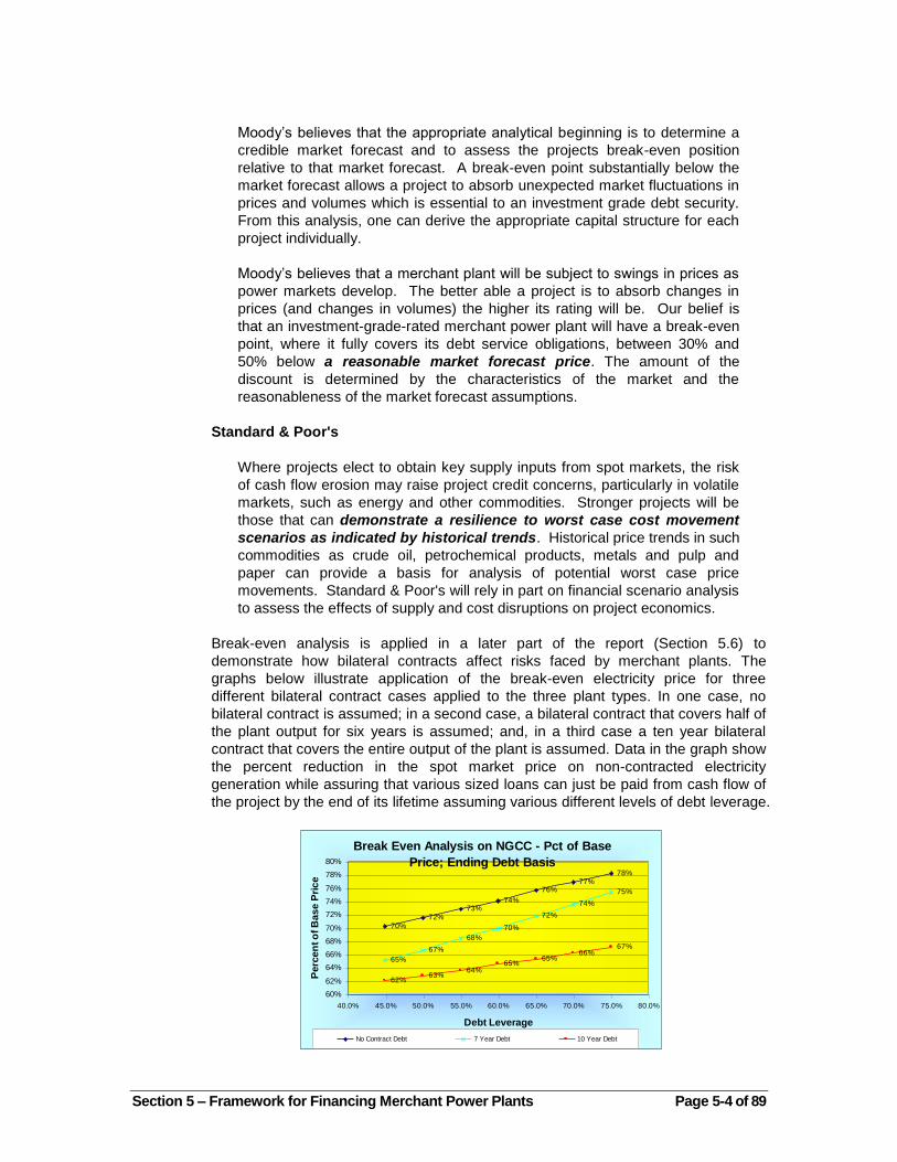
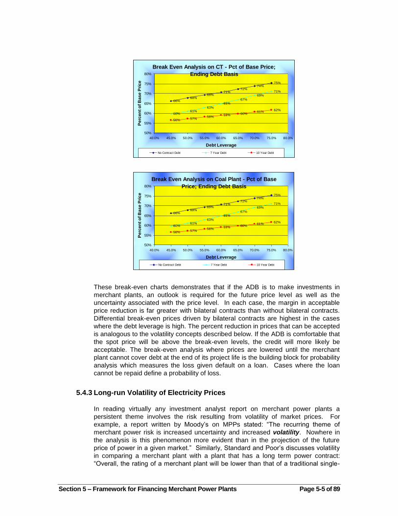
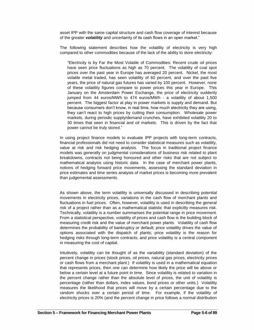
Break-even analysis is applied in a later part of the report (Section 5.6) to
demonstrate how bilateral contracts affect risks faced by merchant plants. The
graphs below illustrate application of the break-even electricity price for three
different bilateral contract cases applied to the three plant types. In one case, no
bilateral contract is assumed; in a second case, a bilateral contract that covers half of
the plant output for six years is assumed; and, in a third case a ten year bilateral
contract that covers the entire output of the plant is assumed. Data in the graph show
the percent reduction in the spot market price on non-contracted electricity
generation while assuring that various sized loans can just be paid from cash flow of
the project by the end of its lifetime assuming various different levels of debt leverage.
Break Even Analysis on NGCC - Pct of Base
Price; Ending Debt Basis
70%
72%
73%74%
76%77%
78%
65%
67%
68%
70%
72%
74%
75%
62%63%
64%65%
65%66%
67%
60%
62%
64%
66%
68%
70%
72%
74%
76%
78%
80%
40.0% 45.0% 50.0% 55.0% 60.0% 65.0% 70.0% 75.0% 80.0%
Debt Leverage
Perc
en
t o
f B
as
e P
ric
e
No Contract Debt 7 Year Debt 10 Year Debt
Section 5 – Framework for Financing Merchant Power Plants Page 5-5 of 89
Break Even Analysis on CT - Pct of Base Price;
Ending Debt Basis
66%68%
69%71%
72%74%
75%
60%61%
63%
65%67%
69%71%
56% 57%58%
59% 60%61%
62%
50%
55%
60%
65%
70%
75%
80%
40.0% 45.0% 50.0% 55.0% 60.0% 65.0% 70.0% 75.0% 80.0%
Debt Leverage
Pe
rce
nt
of
Ba
se
Pri
ce
No Contract Debt 7 Year Debt 10 Year Debt
Break Even Analysis on Coal Plant - Pct of Base
Price; Ending Debt Basis
66%68%
69%71%
72%74%
75%
60%61%
63%
65%67%
69%71%
56% 57%58%
59% 60%61%
62%
50%
55%
60%
65%
70%
75%
80%
40.0% 45.0% 50.0% 55.0% 60.0% 65.0% 70.0% 75.0% 80.0%
Debt Leverage
Pe
rce
nt
of
Ba
se
Pri
ce
No Contract Debt 7 Year Debt 10 Year Debt
These break-even charts demonstrates that if the ADB is to make investments in
merchant plants, an outlook is required for the future price level as well as the
uncertainty associated with the price level. In each case, the margin in acceptable
price reduction is far greater with bilateral contracts than without bilateral contracts.
Differential break-even prices driven by bilateral contracts are highest in the cases
where the debt leverage is high. The percent reduction in prices that can be accepted
is analogous to the volatility concepts described below. If the ADB is comfortable that
the spot price will be above the break-even levels, the credit will more likely be
acceptable. The break-even analysis where prices are lowered until the merchant
plant cannot cover debt at the end of its project life is the building block for probability
analysis which measures the loss given default on a loan. Cases where the loan
cannot be repaid define a probability of loss.
5.4.3 Long-run Volatility of Electricity Prices
In reading virtually any investment analyst report on merchant power plants a
persistent theme involves the risk resulting from volatility of market prices. For
example, a report written by Moody’s on MPPs stated: ―The recurring theme of
merchant power risk is increased uncertainty and increased volatility. Nowhere in
the analysis is this phenomenon more evident than in the projection of the future
price of power in a given market.‖ Similarly, Standard and Poor’s discusses volatility
in comparing a merchant plant with a plant that has a long term power contract:
―Overall, the rating of a merchant plant will be lower than that of a traditional single-
Section 5 – Framework for Financing Merchant Power Plants Page 5-6 of 89
asset IPP with the same capital structure and cash flow coverage of interest because
of the greater volatility and uncertainty of its cash flows in an open market.‖
The following statement describes how the volatility of electricity is very high
compared to other commodities because of the lack of the ability to store electricity:
―Electricity is by Far the Most Volatile of Commodities: Recent crude oil prices
have seen price fluctuations as high as 70 percent. The volatility of coal spot
prices over the past year in Europe has averaged 20 percent. Nickel, the most
volatile metal traded, has seen volatility of 60 percent, and over the past five
years, the price of natural gas futures has varied by 100 percent. However, none
of these volatility figures compare to power prices this year in Europe. This
January on the Amsterdam Power Exchange, the price of electricity suddenly
jumped from 44 euros/MWh to 474 euros/MWh - a volatility of about 1,500
percent. The biggest factor at play in power markets is supply and demand. But
because consumers don’t know, in real time, how much electricity they are using,
they can’t react to high prices by cutting their consumption. Wholesale power
markets, during periodic supply/demand crunches, have exhibited volatility 20 to
30 times that seen in financial and oil markets. This is driven by the fact that
power cannot be truly stored.‖
In using project finance models to evaluate IPP projects with long-term contracts,
financial professionals did not need to consider statistical measures such as volatility,
value at risk and risk hedging analysis. The focus in traditional project finance
models was generally on judgmental considerations of business risk related to plant
breakdowns, contracts not being honoured and other risks that are not subject to
mathematical analysis using historic data. In the case of merchant power plants,
notions of hedging forward price movements, assessing the standard deviation in
price estimates and time series analysis of market prices is becoming more prevalent
than judgemental assessments.
As shown above, the term volatility is universally discussed in describing potential
movements in electricity prices, variations in the cash flow of merchant plants and
fluctuations in fuel prices. Often, however, volatility is used in describing the general
risk of a project rather than as a mathematical statistic that explicitly measures risk.
Technically, volatility is a number summarises the potential range in price movement.
From a statistical perspective, volatility of prices and cash flow is the building block of
measuring credit risk and the value of merchant power plants. Volatility of cash flow
determines the probability of bankruptcy or default; price volatility drives the value of
options associated with the dispatch of plants; price volatility is the reason for
hedging risks through long-term contracts; and price volatility is a central component
in measuring the cost of capital.
Intuitively, volatility can be thought of as the variability (standard deviation) of the
percent change in prices (stock prices, oil prices, natural gas prices, electricity prices
or cash flows from a merchant plant.) If volatility is used in a mathematical equation
that represents prices, then one can determine how likely the price will be above or
below a certain level at a future point in time. Since volatility is related to variation in
the percent change rather than the absolute level of prices, the unit of volatility is
percentage (rather than dollars, index values, bond prices or other units.) Volatility
measures the likelihood that prices will move by a certain percentage due to the
random shocks over a certain period of time. For example, if the volatility of
electricity prices is 20% (and the percent change in price follows a normal distribution

Section 5 – Framework for Financing Merchant Power Plants Page 5-7 of 89
without mean reversion), then there is a 67% chance that a random movements in
prices over the next year will result a price that is within 20% of the current price.
Similarly, there is a 33% chance that the next year price level will be more than 20%
higher or lower than the current price. Mathematical equations for volatility are
described in Appendix 3.
Volatility can be computed for annual, monthly, daily or hourly prices. In the credit
analysis of MPPs, annual volatility is most important. Due to the fact that electricity
cannot be stored, short-term volatility of prices that cause cash flows to increase or
decrease in certain hours, days or months are less important than long-term price
movements. Annual price volatility in various markets around the world is shown in
the graph below. Mathematical techniques used in making the volatility calculations
are described in Appendix 3. The source of raw data is discussed in Part 3 of the
MPP report. Annual price volatility is highest for the Victoria state in Australia,
Nordpool and Chile and is lowest for Argentina and the UK. High volatility is driven
by hydro variability and changes in supply while low volatility is characterised by
markets with surplus capacity.
Annual Volatility
13.1%
39.6%
24.7%
20.9%
48.2%
31.4%
25.1%
39.1%
14.8%
0.0% 10.0% 20.0% 30.0% 40.0% 50.0% 60.0%
UK
Chile
NEPOOL
Aus-NSW
Aus-Vic
Aus-SA
Aus-SNOWY
Nordpool
Argentina
To illustrate the importance of volatility parameters in analysis of investment
decisions, the table below shows how different levels of annual volatility in the price
of electricity affect the probability that a project finance loan will default. We include
this table before fully explaining the process to compute probability of default to show
the practical way in which volatility affects decision making. The table shows that if
the annual volatility of electricity prices is 25% the probability that a loan on an NGCC
plant will not be paid back to banks (the probability of default) is 32%, while if the
annual volatility is 35%, then the probability of not being paid is 49% and if the annual
volatility is 15%, the probability of default is 11%. Much of the remainder of the report
describes how the probability of not being paid can be influenced by signing long-
term contracts, using forward markets to lock in prices, negotiating flexible supply
contracts, incorporating financial covenants in loan agreements, changing the debt
leverage of the plant, using mezzanine and subordinated financing and purchasing
insurance.
The table illustrates that the probability of default is lower for a capital intensive coal
plant than a fuel intensive NGCC plant because the coal plant has a larger capital
base and therefore can accept a larger decline in prices before a default occurs. If

Section 5 – Framework for Financing Merchant Power Plants Page 5-8 of 89
the price of fuel varies with the price of electricity, the probability of loss declines.
Much of the remainder of the report focuses on NGCC plant to highlight the effects of
volatility on the underwriting of MPP credit.
5.4.4 Monte Carlo Simulation in Analysis of MPPs
Once volatility is computed, a method must be developed that translates volatility into
measurement of risk. A common way to apply volatility in measuring the risk
associated with cash flow is to use a process known as Monte Carlo simulation.
Monte Carlo simulation can be applied to measure the probability that a loan will not
be repaid and it can also quantify the deviation in free cash flow. The above tables
that present the probability of default using different debt structures and different
volatility assumptions were developed using Monte Carlo simulation. The fact that
Monte Carlo simulation is used in practice to evaluate merchant power plants is
discussed in the following quote by Paul Ashley, a project finance expert:
―Given plausible assumptions for key risk drivers (for example, volatility of gas
prices), the ratings are then built around simulating cash flows and debt coverage
for individual projects. These simulations can then determine probability and loss
distribution and directly observe the impact on cash flows and riskiness of a
particular transaction structure under different market environments.
The parameterization of the rating simulations combines market data and expert
judgment in a structured way that allows transparency and consistency in risk
evaluation without losing the ability to capture the specifics of a transaction
structure.‖
Monte Carlo simulation uses random numbers and a mathematical process to
construct a range of possible prices over different time periods. The way in which
random draws affect prices depends on the volatility parameter – the higher the
volatility the more the potential variation in prices. Technical details that describe how
Monte Carlo simulation can be applied in practice are described in Appendix 1.
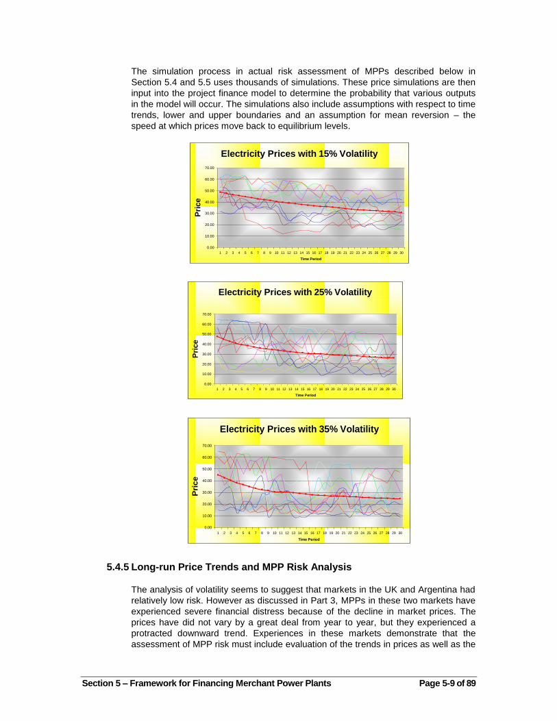
To illustrate how the Monte Carlo simulation process works, three graphs are
presented below that show selected price patterns that are generated by assuming
an annual volatility of 15%, 25% and volatility of 35%. The 15% volatility assumption
roughly corresponds to markets in Argentina, the UK and the US while the higher
volatility parameter corresponds to markets in Scandinavia, Chile and parts of
Australia. Each graph presents ten different price paths generated by random
numbers.
Section 5 – Framework for Financing Merchant Power Plants Page 5-9 of 89
The simulation process in actual risk assessment of MPPs described below in
Section 5.4 and 5.5 uses thousands of simulations. These price simulations are then
input into the project finance model to determine the probability that various outputs
in the model will occur. The simulations also include assumptions with respect to time
trends, lower and upper boundaries and an assumption for mean reversion – the
speed at which prices move back to equilibrium levels.
Electricity Prices with 15% Volatility
0.00
10.00
20.00
30.00
40.00
50.00
60.00
70.00
1 2 3 4 5 6 7 8 9 10 11 12 13 14 15 16 17 18 19 20 21 22 23 24 25 26 27 28 29 30
Time Period
Pri
ce
Electricity Prices with 25% Volatility
0.00
10.00
20.00
30.00
40.00
50.00
60.00
70.00
1 2 3 4 5 6 7 8 9 10 11 12 13 14 15 16 17 18 19 20 21 22 23 24 25 26 27 28 29 30
Time Period
Pri
ce
Electricity Prices with 35% Volatility
0.00
10.00
20.00
30.00
40.00
50.00
60.00
70.00
1 2 3 4 5 6 7 8 9 10 11 12 13 14 15 16 17 18 19 20 21 22 23 24 25 26 27 28 29 30
Time Period
Pri
ce
5.4.5 Long-run Price Trends and MPP Risk Analysis
The analysis of volatility seems to suggest that markets in the UK and Argentina had
relatively low risk. However as discussed in Part 3, MPPs in these two markets have
experienced severe financial distress because of the decline in market prices. The
prices have did not vary by a great deal from year to year, but they experienced a
protracted downward trend. Experiences in these markets demonstrate that the
assessment of MPP risk must include evaluation of the trends in prices as well as the

Section 5 – Framework for Financing Merchant Power Plants Page 5-10 of 89
volatility of prices. In other words, the long-term trends in prices affect the financial
risk more than the volatility of prices. The next two sections discuss how the ADB can
make estimates of the long-term trend in prices using marginal cost analysis and
forward price simulation.
To develop forward price trends, outlooks must be established for energy prices,
capacity prices, and capacity expansion. The price outlooks are required for both the
individual investment analysis and for the country strategic plans. For the individual
MPP transactions, the ADB must evaluate whether long-term prices can support
plant investments. For the country strategic plans, the ADB must consider how policy
options affect long-term energy and capacity prices. In describing the process of
making long-term projections, we first discuss long-term marginal cost analyses and
then forward pricing simulation models derived from forecasts of supply and demand.
Requirements to forecast electricity prices in assessing the credit risk of an
investment are described in the following statement made by Moody’s:
In a deregulated market, electricity will trade and be priced as a commodity and
generating plants will face changes in volumes and prices which will result in
boom and bust cycles. Market participants will react to these cycles with
decisions to expand or contract capacity, which will fuel more cycles. Managers
will be forced to forecast demand and will face the repercussions of both over-
forecasting, as excess capacity will lower prices and returns, and under-
forecasting, as a capacity shortage will invite new competitors and/or re-
regulation. And competitors will exploit poor management decisions in a way that
was impossible in a regulated environment.
Price outlooks used to evaluate individual transactions and used in quantifying policy
frameworks are often developed from complex simulation models that rely on large
databases. A mistake made in the relatively short history of merchant power has
been to rely on the complex models without questioning the general plausibility of the
results and establishing a reference point for the projections. To avoid repeating this
mistake in projecting price trends, the ADB should compute long-run marginal costs
as a reference point in developing more complex forecasts. Therefore, before
describing forward models, we discuss how long-run marginal cost can be calculated
to provide the ADB with a tool to evaluate the general plausibility of complex model
results. The following two statements by Moody’s illustrate the need for a reference
point in making electricity price forecasts:
In Moody’s opinion, project economics associated with long-term power
market forecasts should be viewed sceptically. Over the short- to-
intermediate term, the introduction of new generating technology into today’s
electrical grids will almost invariably provide project owners with an opportunity
for exceptional risk-adjusted rates of return. But over the longer term, new
entrants, which offer similar — or perhaps better — technology, will inevitably
drive market prices down, potentially undermining the economic rationale of even
what would now appear to be the most favourably positioned projects. What’s
more, the long-term prediction of power prices — and thus a specific project’s
ability to retain or add customers — is heavily dependent upon inherently
uncertain assumptions regarding a particular market’s demand and supply
characteristics; regulatory and political environments; and the economic rationale
of new investors.
It is important to emphasize that the power rate consultants’ computer models

Section 5 – Framework for Financing Merchant Power Plants Page 5-11 of 89
generally employ linear programming techniques and are extremely complicated.
By the time Moody’s issues a rating, Moody’s will understand in great detail the
power rate consultant’s assumptions and approach. However, Moody’s cannot
know the computer model’s detailed logic. Thus, there is a black box character
to these models.
5.4.6 Long-run Marginal Cost and Forward Price Projection
A starting point in analysis of electricity trends is computation of the long-term
marginal cost. Long-term marginal cost is a conceptual tool that explains why prices
should converge to certain levels and should be part of the underwriting process for
an MPP. An understanding of the marginal cost of electricity is essential to analysis
of the forward pricing and plant valuation in any industry. Assumption that prices will
indefinitely be below or above marginal cost by a wide margin is not reasonable
without assuming barriers to entry or market intervention that should not be
sustainable. Credit analysis for MPPs should therefore compare long-run marginal
cost with long-term price forecasts to assess whether the forecasts are reasonable.
In addition, development of long-run marginal cost analysis is a useful tool in many
other aspects of the analysis of market frameworks. For example, long-run cost
analysis can be used to assess whether retail rates are set at levels that provide an
appropriate consumption incentive; whether significant market power is present; and,
whether prices established in long-term contracts are reasonable.
In evaluating investments and policy with respect to merchant plants, the ADB should
have a tool that evaluates the long-run marginal cost of electricity. A
misunderstanding of long-run marginal costs has caused problems in the underwriting
of MPPs. For example, price forecasts in Argentina assumed that an inefficient
capacity mix would remain in place, neglecting the downward trend toward the long-
run cost defined by more efficient capacity. Long-run marginal cost is important
because at some point rational economic behaviour must exist. This point is made by
Peter Rigby of Standard and Poor’s:
Generally most models assume rational behaviour by market participants,
and that a system will operate economically in the most efficient manner,
given the physical constraints of the system. Unfortunately, market
participants do not always behave rationally or uniformly – fortunately they
do not behave recklessly either…Underlying every model is the
assumption that the markets will operate in a perfect long-term equilibrium,
and that they will price electricity at the marginal cost of production.
Unfortunately the reality of energy markets appears much different.
Equilibrium lasts momentarily at best. A sudden change in fuel prices, a
change in system load, or the presence of a new power station will upset
the equilibrium.
A model for determining long-run marginal cost for purposes of evaluating merchant
plants is presented in Appendix 3. This model combines the tools discussed above –
carrying charge rates from the project finance model, plant costs from the case study
discussion and a load duration curve for the Philippines. We have included the long-
run marginal cost model as part of the tool-kit for evaluating merchant power plants
because, although it is simple, long-run marginal cost can be an effective tool in
assessing whether complicated forward pricing models with multi-regional
transmission constraints, volatility premiums, price spikes and Monte Carlo simulation
of plant outages are producing reasonable results. The long-run marginal cost in

Section 5 – Framework for Financing Merchant Power Plants Page 5-12 of 89
evaluating price forecasts described in Appendix 3 begins with analysis of prices in
current markets. Next, long-run marginal cost is computed from load profiles and cost
characteristics of new plants. Prices derived from long-run marginal cost are high
enough to promote construction of an efficient mix of new plants. Finally, with current
prices and equilibrium prices established, evaluation of merchant plants using this
framework must address how and
when prices will move from
current market levels to
equilibrium.
Long-run marginal costs can be
used to evaluate the likely
direction of future prices. If
current prices are higher than the
price level that covers the cost of
building new capacity, you would
expect the prices to come down.
This situation is illustrated by the
case of Argentina and the
Northeast US, where price levels
at the inception of the market
were above the prices required for
construction of new combined
cycle plants. On the other hand, if
current price levels do not allow
profitable construction of new
plants, you should expect prices
to increase.
The marginal cost framework can be used to evaluate the effects of the level of
capacity and/or the mix of generating plants in a country not being at an equilibrium
level. In cases where there is too much capacity, too little capacity, or the wrong mix
of capacity, prices will not be at equilibrium levels and private developers can
potentially profit from realizing prices that do not reflect the cost of new building plants.
For example, if there is too much peaking capacity in a region relative to the
economic optimum, the net cost of capacity for base load plants – after recovery of
variable costs from off-peak prices -- is less than the annualized cost of a peaking
plant.
The two tables below shows the computation of long-run marginal costs in various
scenarios. The first table demonstrates prices that result from computation of
marginal cost if the market is in equilibrium and the carrying charges are derived from
debt leverage of 60%. At a load factor of 62%, representing the average load factor of
the system, the long-run marginal cost using the three representative plants is
$38/MWH. (This long-run marginal does not include an assumption of a declining
price trend. With a declining price trend, the long-run marginal cost is consistent with
the $45/MWH assumption used in the project finance model.) The table illustrates that
different plants face different prices because of the time at which dispatch occurs. If a
plant operates at 100% load factor, the price faced by the plant is $34/MWH instead
of $38/MWH.
The second table shows the effect of different carrying charges and technology
assumptions on the long-run marginal cost. With higher carrying charges, the long-run
equilibrium price increases because prices must cover higher costs of capital. If the
Example of Using Long-Run Marginal Cost to Evaluate Price Forecasts in
MPP Proposals In thinking about the forward price model presented below suppose an ADB analyst must review a forecast of electricity market prices made by a market price consultant for a plant in Vietnam. The ADB staff must review the forward price forecast without a fancy hour-by-hour ―multi-regional‖ simulation model. In reviewing the market price forecast, a place to start is evaluation of the level of current prices. Next, the level of prices at ―equilibrium‖ could be computed where the price just covers the cost of constructing and operating new capacity and where an optimal mix of resources exists in the market. Finally, an assessment could be made about how prices will move from current levels to long-run marginal cost that defines equilibrium levels. While this simple approach may not address specific plant outages, variability in price spikes, changes in hydro conditions profitability of individual existing plants or generating unit ramp rates, the simple framework includes evaluation of actual prices, how fuel prices and changes in productivity that affect long-term prices, and behavior of merchants that affect how prices will move to equilibrium.

Section 5 – Framework for Financing Merchant Power Plants Page 5-13 of 89
carrying charge increases because of lower leverage, the mix of capacity and the
long-run marginal cost increase from $38.81/MWH to $45.50/MWH – an increase of
17%. In addition, the capacity mix changes and low capital cost unit peaking plants
are a far higher proportion of the total capacity.
5.4.7 Forward Price Simulation Models in Analysis of MPPs
Long-run marginal cost does not consider that construction behaviour of developers
is somewhat unpredictable and may arguably be irrational in the short-term. If the
ADB were to invest in merchant plants, forward pricing simulation models would have
to be reviewed. A forward price simulation model can be used to demonstrate how
risks associated with supply and demand; how different market frameworks affect
costs and prices; drivers, construction of volatility, data requirements and technical
heat rate issues. Unlike project finance valuation and financial modelling, market
price simulation is very difficult to accomplish with spreadsheet analysis because of
hour-by-hour dispatch, maintenance outage modelling, hydro operation, energy
margin computations and optimization of new capacity. The following quote
demonstrates how Moody’s uses forward price simulation models developed by
market consultants in evaluating merchant plant risks:
The market study is intended to provide an assessment of the market structure
and behaviour of participants that then allows a credible projection of market
prices. The predictive power of a market study is only as good as the
assumptions that underlie the analysis. Since the ultimate goal of the market
study is to predict the price of power, most studies use economic forecasts to
derive demand and focus on the supply elements.
Moody’s relies on issuers and market consultants to provide us with forecasts of
the future price of power. The key to this analysis is the cost of supply at any
given level of demand. It is this underlying cost of all market suppliers of power
that will be determinate in the market price of power. Consequently, a merchant

Section 5 – Framework for Financing Merchant Power Plants Page 5-14 of 89
plant’s cost position relative to its current and potential competitors is one of the
primary factors in assigning a rating. While determining the costs of a single plant
is rather straightforward, determining its position relative to others and how each
party may bid into an open power market is more complex.
Forward price simulation models project market clearing prices using estimates of
hourly loads and plant data. The plant data includes fuel prices, maintenance
outages, variable operation and maintenance, plant heat rates, existing thermal
capacity, pumped storage hydro capacity and transmission constraints on imports
and exports for a market region. The databases of loads and power plants are used
in a dispatch module that simulates the hourly operation of power plants. Forward
price models differ from the simple marginal cost models described above in three
respects. First, the models account for existing supply and predict prices when the
market is not in equilibrium – when there is excess or deficient supply and when the
capacity mix is not optimal. Second, the models include capacity prices and account
for the relationship between capacity and energy markets. Third, the models can
simulate the volatility of prices as well as the expected level of prices.
To introduce forward price models, we present alternative scenarios for the
Philippines case study. In the first scenario, the assumption is made that capacity
reaches equilibrium as demand grows. In the second scenario, developers are
assumed build more capacity than is implied by equilibrium and in the third case
demand grows faster than the base case. This type of analysis of merchant plants is
representative of actual analysis as illustrated in the following quote:
Power rate consultants assume long term generation demand and supply will be
in equilibrium. Moody’s agrees with that assumption, but assumes that in certain
years overbuilding or an economic recession will create an excess generation
capacity situation. A good example of a current overbuild situation is northern
Chile where burgeoning supply far exceeds expected demand. Other examples
may evolve in New England or near Chicago where significant numbers of new
plants have been announced.
The two graphs below illustrate how price trends are dependent on outlooks for the
behaviour of developers. The first graph shows an overbuild scenario where
developers build more capacity than is justified in order to earn their cost of capital.
The second graph shows a situation where demand increases no overbuild occurs.
The first chart shows that after a capacity overbuild, it can take many years before
the market reaches equilibrium, which can have several financial consequences to an
MPP. The two graphs illustrates that the time it takes to reach equilibrium after an
over-build scenario can dramatically affect the value and the credit quality of a
merchant plant.

Section 5 – Framework for Financing Merchant Power Plants Page 5-15 of 89
Annual Energy Market Clearing Price
15.11 15.31
17.24
20.26
22.44
25.87
22.8421.26 20.89 21.13
21.8422.77
23.7024.79
25.9427.29
28.6930.22
31.93
33.77
35.69
37.90
40.47
43.20
17.82 18.37
21.34
29.71
34.12
36.15
32.23
28.2226.83 26.77
27.6728.89
31.5433.04
34.7536.47
38.35
40.54
42.86
45.27
48.18
51.60
55.26
12.93 12.8613.90
12.53 13.05
17.56
15.27 15.63 16.09 16.58 17.1317.83
18.5319.34
20.2121.26
22.4123.63
24.9626.41
27.9329.57
31.46
33.45
30.11
-
10.00
20.00
30.00
40.00
50.00
60.00
1995 1996 1997 1998 1999 2000 2001 2002 2003 2004 2005 2006 2007 2008 2009 2010 2011 2012 2013 2014 2015 2016 2017 2018
Year
AverageOn-PeakOff-PeakActual Average
Annual Energy Market Clearing Price
15.11 15.3117.24
20.26
24.56
27.4626.15 26.49
27.3729.16 29.56
31.3432.76
34.5436.42
38.1740.32
41.87
44.43
47.0849.45
51.92
54.68
57.25
17.82 18.37
21.34
29.71
38.79 39.46 39.64 39.3540.25
43.17 42.7345.07
48.7750.92
52.5154.78
55.66
58.31
61.0463.25
65.54
68.56
71.32
12.93 12.8613.90
12.53 13.11
17.80
15.32 16.1617.02
17.8918.97
20.3021.63
23.0924.74
26.6328.68
30.76
33.26
35.83
38.33
40.95
43.50
45.9246.59
-
10.00
20.00
30.00
40.00
50.00
60.00
70.00
80.00
1995 1996 1997 1998 1999 2000 2001 2002 2003 2004 2005 2006 2007 2008 2009 2010 2011 2012 2013 2014 2015 2016 2017 2018
Year
AverageOn-PeakOff-PeakActual Average
5.5 Risk Assessment of MPPs
5.5.1 Introduction
Given the volatility of electricity prices and the potential for downward movement in
prices one may wonder whether why any investment – particularly debt investment --
is made in MPPs. However, according to Standard and Poor’s: ―merchant power
plants, mining projects, and oil and gas projects that produce and sell volatile
commodities have raised billions of dollars of non-recourse rated project finance debt
without the benefit of traditionally structured off take contracts.‖ The question
therefore is not whether MPPs are too risky, but rather how to measure risk so that
ADB loans, equity investments and insurance products are appropriately priced to
reflect the risk.
Analysing risks in a rigorous manner is the central issue the ADB must address when
investing in the merchant power industry. Risk analysis already been considered in
the discussions of volatility, break-even analysis, sensitivity analysis, probability of
default and carrying charges. In this section we describe how some of the most
important risks faced by MPPs can be quantified. These risks include demand
variability, fuel constraints and price volatility, hydro yield variation, developer
behaviour and the uncertainty in the productivity and reliability of new technologies.
The discussion of various different risks allows the ADB to evaluate different MPP
investments in various countries. For example, if a country has relatively low
demand variability, the ADB can consider how the low demand risk affects cash flow
volatility and what underwriting and pricing standards should be implemented.
Section 5 – Framework for Financing Merchant Power Plants Page 5-16 of 89
Similarly, if a country has high hydro volatility, the ADB can determine how debt
leverage, debt service benchmarks and policy recommendations should be adjusted
relative to countries without significant hydro risk.
Financial economists often separate risks into various categories when evaluating
investments under uncertainty. A first risk category -- market risks – consists of those
risks driven by variables such as commodity prices and interest rates. These risks
can often be hedged through forward contracts and other derivatives. A second risk
category -- strategic risks -- is associated with the business activities embarked upon
by a company. These risks must be incurred by a business in order for the company
to earn economic profit. Other categories of risks include regulatory risks, financial
risks, contract risks and construction risks. In the remainder of the report we discuss
four general risks faced by merchant power plants. These include: (1) market risk
including the sale price and dispatch of electricity and the cost of fuel; (2) project risk
including technology, construction and operating risks; (3) strategic risk driven by
decisions made by MPPs; and, (4) risks associated with bilateral contracts.
Each of the risks affects the question of how much future revenues derived from
prices of electricity and dispatch quantities faced by an MPP will deviate from
expected levels. Risks may affect both the volatility around prices for a short period
and long-term trends in the price of electricity. Issues associated with physical
dispatch, price volatility and price trends for MPPs overwhelm construction cost,
operation and maintenance and interest rate risks that are important in underwriting
plants with long-term contracts. For each risk category we first describe how the risk
affects prices on from a qualitative standpoint. Next, we discuss mathematical
techniques that can be used to measure the risks. Finally, we consider how the risk
can be quantified in terms of the cash flows and credit quality of MPPs.
5.5.2 Market Risks from Electricity Demand Uncertainty
In making investments in merchant power plants, the ADB will need to develop a
framework to project the range in possible prices. One method is to make
judgemental assessments as described above. A second method involves applying
estimates of the volatility of demand, fuel price and supply factors from objective
historic data and evaluating the volatility of future prices. Unlike plants with long-term
purchase contracts, merchant plants must absorb risks of demand fluctuations, fuel
prices, developer behaviour, plant outages, hydro variation and other factors.
Volatility estimates can be developed for all of these inputs and the volatility of power
prices can be evaluated.
We begin the discussion of specific risks by considering market risks that are outside
of the control of investors in merchant plants. Three risks that affect the cash flow of
merchant plants and were insulated from IPP’s with long-term contracts include risks
associated with demand growth, risks that occur because of fuel price swings, and
risks that arise from changes in the hydro energy from river flow fluctuations. The
following statement demonstrates how market risk affects the credit rating of an MPP:
In an era of competitive power when merchant generators are assuming risks of
price and dispatch (volume) ….the presence of electricity market risk in a project
is often a constraint in obtaining an investment-grade rating, especially for single-
asset plants that have no portfolio diversification.
Demand risk affects MPPs in two important ways. First, the level of demand can

Section 5 – Framework for Financing Merchant Power Plants Page 5-17 of 89
affect the amount by which MPPs are dispatched. Second, the level of demand
relative to supply can dramatically affect prices for long periods of time. An example
of the first type of risk – capacity factor variation -- is the possibility that a peaking
plant will not run because of moderate weather. An example of risks associated with
supply and demand imbalance is the risk that demand will below expected levels and
an MPP will face low prices for an extended period of time because of excess
capacity in the market.
The effects of volume risk are illustrated using the combustion turbine case study. In
the first case there is no uncertainty associated with demand risk and the price
uncertainty uses the 25% volatility assumption above. In the second case, volume
increases or decreases in a random manner representing the way in which extreme
weather affects the dispatch of peaking plants. The first graph shows the distribution
of the present value of project cash flows with and without volume risk. The table
below the chart demonstrates that volume risk more than doubles the credit risk of
the peaking plant.
Project NPV
0
20
40
60
80
100
120
140
-58586.33 -28120.09 2346.16 32812.41 63278.65 93744.90 124211.15
Range in Value
Nu
mb
er
of
Scen
ari
os
I
Demand risks facing an MPP are very different than demand risks facing plants that
operate in a regulated or stated owned system or plants that have long-term fixed
price contracts. In regulated or state-owned systems, if changes in demand cause
there to be surplus or deficient capacity in a market, higher or lower rates are
generally imposed on consumers. Similarly, if electricity generation plants have fixed
price contracts, the cash flow of the plant does not change when overall demand of
the electricity system changes. This is not the case for merchant plants. In both the
short-run and the long-run the cash flow for a merchant plant depends on how
demand affects the market price and how demand affects the level of dispatch. For a

Section 5 – Framework for Financing Merchant Power Plants Page 5-18 of 89
given level of capacity, if demand is lower than expected, the price and capacity
factor will fall while if demand is higher than expected, the price and the capacity
factor increases. The following statements by investment analysts of MPPs illustrate
the importance of considering demand risks:
Merchant power plants (MPPs) face volume risk. This risk was traditionally
absorbed by the utility, but in an uncontracted world each individual generator will
be subject to the hour-by-hour fluctuations in the demand for power.
A longer-term element of volume risk is the growth of electricity demand in the
area in which a plant can supply power. This analysis is tied to the economic
viability of a city, state or region compared to other areas, and focuses on broad
demographic trends. Likewise, questions regarding individual demand for power
or per capita consumption of power would affect a merchant plant. All of these
questions would need to be answered on a market-by-market basis if there is
more than one merchant generating station, or for the single market in the case
of a single asset generating station.
Demand growth assumptions not only determine assumed electricity needs over
time, they also determine the region’s changing generating plant mix. As
discussed below, given that industry participants expect future new generation
will overwhelmingly take the form of simple cycle or combined cycle gas-fired
plants, regions predicted to experience great demand growth will more quickly
become dominated by gas-fired generation than will regions predicted to
experience slower demand growth. A region’s equipment mix will, of course,
affect that region’s variable and fixed generation cost assumptions.
The way in which an MPP faces demand risk can be demonstrated by the history of
demand fluctuations that have occurred in Asian electricity systems over the past
decade. Part 2 of the MPP report documents the way in which demand changed
because of the Asian crisis. The swings in demand before and after the Asian
economic crisis would have had dramatic effects on spot market prices had
competitive systems been in place. The surplus in capacity that occurred after the
crisis would have depressed prices for many years. A specific example of demand
risk faced by MPPs through unexpected long-term trends is illustrated by the case of
Argentina below. If an MPP had been contemplating an investment in 1977, it may
have been reasonable to anticipate growth of 6% to 7% per year. However, actual
growth turned out to be much lower. The lower growth means that reserves were
much higher than anticipated and that the prices and capacity factors experienced by
cycling and peaking plants would also have been lower than anticipated.
Alternative methods can be used to quantify demand risk including scenario analysis

Section 5 – Framework for Financing Merchant Power Plants Page 5-19 of 89
that incorporates judgement and macro-economic information and statistical analysis
of historic trends that use volatility and simulation. The potential for long-term
changes in demand is driven by the state of the economy and changes in use of
electricity caused by different industry structures. Such changes in long-term trends
are difficult to assess by examining historic trends in sales data. Problems with use of
extrapolation are demonstrated by the Asian crisis wherein changes in electricity
demand would not be predicted from analysis of past trends. In analysing long-term
demand we recommend that the underwriting process begin with statistical analysis
and then used scenario analysis to consider the potential for lower than expected
demand.
Short-term changes in demand create risk in the cash flow of an MPP due to the
manner in which demand changes affect both the spot price and the level of dispatch.
These changes in demand are generally driven by weather as well as changes in
economic activity. If the weather is warmer than expected in the summer, the
demand will generally be higher. In this case, the electricity price and the cash flow
of a merchant plant will also be higher. The weather driven changes in demand can
be quantified with statistical analysis through applying volatility statistics to the long-
tem demand projections. The volatility statistic is computed in the same manner as
for prices described in Appendix 1, except that the data for making the mathematical
calculations is first seasonally adjusted.
To incorporate demand risks into the underwriting process for an MPP, demand
forecasts that incorporate risk must be included in evaluation of price trends.
Inclusion of risk involves accounting for both the potential for structural changes in
economic activity and short-term volatility. The long-term volatility is generally
measured with scenario analysis while short-term risk is driven by volatility
measurement. An example of how different long-term price projections and short-
term volatility can be used to measure risk is illustrated in the graph below which
applies Monte Carlo simulation to reflect the short-term weather related volatility. As
with the graphs that apply volatility to market prices shown in Section 5.4.4, only a
few of the multiple scenarios are shown on the graph.
Peak Load Scenarios
30,000
32,000
34,000
36,000
38,000
40,000
42,000
44,000
2004 2005 2006 2007 2008 2009 2010 2011 2012 2013 2014 2015 2016 2017 2018 2019 2020 2021 2022 2023
Once the long-term demand scenarios and the volatility parameters are established,
the data becomes an input to forward price simulation models. Using the example in
the graph above, the variation in demand data would drive the computation of price
and dispatch in many applications of the forward price simulation model. Since
multiple demand paths result from application of the volatility in the demand analysis
and from construction of alternative long-term scenarios, and since each demand
path results in a different price path and capacity factor projection, multiple potential

Section 5 – Framework for Financing Merchant Power Plants Page 5-20 of 89
MPP cash flow projections result from this process.
5.5.3 Market Risks from Fuel Price Uncertainty
A market risk faced by MPP investors other than demand risk involves the possibility
that fluctuations in the price of fuel can negatively impact the cash flow of a plant.
Changes in the price of fuel price affect the MPP risks because of the manner in
which fuel prices affect both revenues and operating costs. The reason fuel price risk
affects revenues is illustrated by the way profit margin earned on from a merchant
coal plant depends on gas prices because of the way gas prices affect electricity
prices. Alternatively, the profit margin on a gas plant can be affected by the price of
gas in hours when the price of electricity is driven by the oil price. Fuel price risk is
discussed in the following statement by Moody’s:
The assumptions regarding fuel costs are very important to a system that has a
variety of plants powered by different fuel types. If a fuel is considered to be ―on
the margin‖ it is the system marginal price setting plant and therefore, as its fuel
costs go up, so does the price of electricity in that market. With regard to the
general level of fuel prices, Moody’s looks at gas prices in market studies since
gas is tending to become the system marginal fuel in many markets for an
increasing percentage of the time. A contentious assumption with market studies
in general is the fact that the price of natural gas will increase at a rate above the
general rate of inflation. This accelerated pace of price increases is attributed to
the greater demand for natural gas as a more environmentally friendly fuel
relative to other fossil fuels and to transportation constraints in markets of high
demand.
In underwriting MPP loans, the ADB must account for the manner in which fuel price
risk occurs in different electricity systems. In some countries the predominant fuel
may be coal with very low price variation while in other countries there may be
diversity in fuel where the price of oil drives spot prices in some hours, the price of
gas drives the market price in other hours and the price of coal influences price in off-
peak hours. In the latter situation, the ADB must account for how price variation
influences both the revenues and the operating costs of an MPP.
Long-term trends and the volatility of fuel prices can be gauged in a similar manner
as the analysis of electricity prices above. In some cases, forward markets exist for
fuel price as is the case with natural gas prices in the US. Forward prices can be
used as the basis for making projections of long-term prices. In cases where forward
markets for fuel exist, options are also often traded. The price of these traded options
can be used to derive what the market thinks future price volatility will be.
Quantification of fuel price risk effects on the cash flow of an MPP can be
accomplished using the tools discussed above involving volatility, price trends and
simulation. As is the case for incorporation of demand risk in MPP analysis, the
representation of fuel price risk is entered into forward price simulation models. Once
trends and the volatility of fuel is input in forward price models, the manner in which
fuel price volatility affects the fuel cost, dispatch level and the market price faced by
an MPP can be evaluated. The resulting cash flow volatility can be combined with
other sources of risk including demand risk to assess the distribution of possible cash
flows that can result from an MPP investment.
5.5.4 Market Risks from Hydro Uncertainty

Section 5 – Framework for Financing Merchant Power Plants Page 5-21 of 89
A third market risk faced by MPP investors involves risks associated with the
variation in energy produced from hydro plants. This is particularly the case with run
of river hydro schemes, or those with relatively small storages. Large hydro storages
can be used to transform volatile inflows into more steady outflows for generation,
even through drought sequences dependent on the operating policies in place. As
with demand risk and fuel price risk, variation in hydro generation affects both market
clearing prices and the dispatch of MPPs. Hydro production is uncertain because of
variation in the river flows driven by weather (e.g. snowfall in mountains and
droughts) and other factors. Since hydro plants have no fuel cost, the production
from hydro will displace the energy production from MPPs that rely on fossil fuels
such as natural gas or oil. Further, since hydro production influences the dispatch
order, hydro risk also influences spot market prices and the revenue earned by an
MPP.
The impact of hydro capacity on price volatility was demonstrated in the discussion of
volatility in Section 5.4.3 above. The manner in which hydro risk affects the dispatch
of an MPP is illustrated by the case of Argentina shown in the graph below. This
graph shows that the capacity factor of hydro plants moves in the opposite direction
to the capacity factor of thermal plants. In those years in which the capacity factor is
higher for hydro plants, the capacity factor is lower for thermal plants as expected
because there is less need to run the thermal plants. The more the hydro capacity
the more the fluctuation in thermal operation that occurs from the variation in hydro
generation. The reduced capacity factor of thermal plants directly affects MPP
revenues as does the lower price that result from increased hydro production.
Hydro and Thermal Capacity Factor in Argentina
20%
25%
30%
35%
40%
45%
50%
55%
1992 1993 1994 1995 1996 1997 1998 1999 2000 2001
Per
cen
tag
e
Hydro Capacity Factor
Thermal Capacity Factor
Unlike risks associated with demand and with fuel prices, hydro risk can be directly
assessed using analysis without additional scenario analysis driven by judgement.
Statistics computed from long term data series of the capacity factor of hydro plants
can compute mean levels of hydro production and the volatility of hydro generation.
For example, in the example of Argentina illustrated above, forward prices analysis
would incorporate the expected capacity factor as well as the volatility of capacity
factor. Hydro risk can be quantified in the underwriting process of an MPP by
incorporating volatility and expected levels in the forward price simulation models.
Once average levels and the volatility of hydro is input in forward price models, the
manner in which hydro volatility influences MPP dispatch and the market price faced
by an MPP is assessed using Monte Carlo simulation. For random draws that imply a
high level of hydro output, the market price declines while for random draws that
drive the hydro output to low level, the MPP financial position improves.

Section 5 – Framework for Financing Merchant Power Plants Page 5-22 of 89
5.5.5 Business Strategy Risks
The most important factor driving the financial meltdown that has occurred in the
merchant power industry around the world has generally not been demand, fuel price
or hydro risks. Instead, financial distress in the UK, Argentina, the US, and Australia
has been driven by the behaviour of MPP developers themselves. In each of these
situations, the amount of capacity built in the market exceeds the amount that keeps
prices at a level that enables a reasonable return to be earned on new capacity.
Surplus capacity resulting from the behaviour of developers in these cases will likely
keep prices below long-run cost for many years. Other risks that can affect prices in
the long-run involve the possibility that changes in the technology and the real capital
cost of new plants will drive prices lower.
Investors in the debt and equity of MPPs have commented on risks related to the
productivity of new plants as follows:
Suppliers of new and cheaper power generation, including more efficient and
technologically advanced units, may represent the greatest threat to an MPPs
cash flow. New supplies may com from Greenfield projects, renovation or
expansion of existing facilities, or additional access to transmission. If new
capacity enters the MPPs service territory, the potential exists for
electricity prices to fall, especially if new generation capacity leads demand
and seeks only to gain market share within a static market. Insofar as new
competitors can produce power more cheaply, MPPs margins may erode as
marginal power costs fall. Moreover, even if new competitors’ cost structures
differ slightly from those of existing generators, the mere fact of the capacity
addition will lower prices, extract market share, or both.
There is considerable uncertainty over where [UK] pool prices will go ….A lot of
merchant power plants are … relying on efficiencies in technology and the low
cost of fuel. But technology improves very quickly and so their relative position in
the pool can change substantially.
In attempting to minimize the risk associated with the future market price of
electricity in the region to be served by the proposed merchant plant, several
considerations must be addressed, including the presence-actual or likely-of
other generation providers within the region, the likelihood of electricity
imports from outside the region, transmission constraints and the future regional
demand for electricity….In making these assessments, one needs to consider
the availability and location of potential generation sites, the financial and
marketing strength of potential competitors, the possibility that any competitor will
utilize a production technology that is more efficient than that of the proposed
plant, and the potential for regulatory changes, such as opening a region to
imported power from neighbouring regions.
Assessing the risk of merchant behaviour and technology changes cannot be
accomplished in a reasonable manner by analysing historic data. Instead, the risks
must be assessed using expert judgement about the industry and by creating
alternative scenarios with respect to new developer behaviour and changes in
technology. The scenarios require knowledge of other developers in the market and
evaluation of the potential for future overbuilds. The way in which overbuilt capacity
can influence market prices is illustrated in the graph which assumes overbuilds of
10%, 20% and 30%. In each case, the demand growth eventually eliminates the

Section 5 – Framework for Financing Merchant Power Plants Page 5-23 of 89
surplus capacity and the market reaches equilibrium when new capacity is required.
The larger the surplus, the lower the market price and the longer it takes for the
market to reach equilibrium.
Risks of potential technology changes that could impact long-term prices can be
evaluated by computing long-run marginal cost as described in Section 5.4.6. The
table below compares long-run marginal cost under four different scenarios. The first
scenario assumes no productivity improvement, the second scenario assumes a 10%
reduction in heat rate, the third scenario assumes a 10% reduction in the real cost of
constructing capacity and the fourth scenario assumes a 10% reduction in both heat
rate and capital cost.
5.6 MPP Credit Analysis and Benchmarks for MPP Financial Structuring
5.6.1 Introduction
Given the above description of general risks facing MPPs we move to the subject of
credit risk which is the basis for underwriting and pricing ADB loans for MPPs.
Analysis of credit risk establishes: (1) a basis for pricing of ADB loans to MPPs; (2)
appropriate financial ratio benchmarks for MPPs; (3) financial structure
enhancements such as covenants and debt service reserves to apply to MPP loans;
and, (4) the nature of bilateral contracts and risk hedging mechanisms that should be
incorporated in MPPs. Our discussion of credit analysis begins with a general
overview of measuring credit risk and pricing loans. Next, tools to measure the credit
risk of MPPs including volatility of cash flow and Monte Carlo simulation are
described. Given these MPP analysis tools, the final parts of this section address
debt service ratio and debt to capital ratio benchmarks the ADB should apply to
prospective MPPs.
5.6.2 Theory and Measurement of Credit Risks and Credit Spreads
Traditionally, credit analysis has involved developing standards to classify loans into
a number of different risk categories. This classification includes bond ratings of
credit rating agencies with letter rankings and credit scoring in banks with numeric
grades. The credit scores should be correlated to the chance of loans not being
repaid (bond rating agencies such as Standard and Poor’s and Moody’s regularly
publish correlations between their bond ratings and the probability of default to
demonstrate the validity of their risk rating systems.) Credit scoring systems
generally involve assessing financial ratios (such as the debt service coverage ratio)
and determining whether key credit risks can be mitigated. Credit risk also accounts
Section 5 – Framework for Financing Merchant Power Plants Page 5-24 of 89
for the collateral and the chances of recovering money once things go wrong.
Modern credit analysis is founded on the notion that risky debt has a payoff structure
that is similar to the seller put option. There is downside risk which can cause
lenders to loose up to the loan amount (driven by the volatility of cash flows) and an
upside payoff that is limited to the credit spread. The option analysis can be used to
directly measure credit spreads – the cost of capital on risky debt – by measuring the
probably of default and the probability of recovering money once a default has
occurred. The latter amount is known as the loss given default. Much of modern
credit analysis involves measuring the probability of default and the loss given default
because the credit spread can be quantified in the following formula:
Credit Spread = Probability of Default x Loss Given Default
In evaluating a power plant with a long-term purchased power contract, the
probability of default is primarily driven by the chances of a default on the power
contract. The reason that the power contract characteristics drive risk assessment is
that other risks are generally moderated by using conventional in constructing the
plant, purchasing insurance for contingencies ranging from business interruption to
political risk, signing O&M contracts to mitigate O&M risk and by using interest rate
swaps to mitigate interest rate risk. With risks transferred to other parties, the risk
that remains is the risk that the purchased power contract will not be honoured
because of financial insolvency of the off-taker. Therefore, a typical rule of thumb in
projects which have a long term power purchase contract is that the project has a
bond rating one notch below the bond rating of the off-taker. In terms of the above
formula, the probability of default on the project is a direct function of the probability
of default on the off-taker.
In contrast to projects with long-term contracts, the probability of loss and the loss
given default cannot be approximated from the bond rating of another company.
Instead, credit analysis of an MPP requires direct assessment of the probability of
loss and the value of collateral if a default occurs. In order to quantify probability of
loss and loss given default the volatility and price trends must be used together with a
project finance model. The greater the volatility of prices and the greater the chances
for downward trends in the market clearing price, the higher the probably of loss and
the higher the loss given default. Further, the loss given default and the probability of
default are directly affected by financial structuring of the MPP related to covenants
and debt service reserves.
5.6.3 Mathematical Assessment of Credit Risk
The theory of establishing credit is straightforward in theory, but in order to be useful, one must be able to reasonably apply the method in practice. Credit spread can be computed for a competitive electricity plant by applying the following step-by-step process:
Step 1: Estimate free cash flow and loss given default through constructing a project finance model that incorporates debt structuring elements such as covenants, debt service reserves and anchor contracts.
Step 2: Develop a measure of probability of default through applying Monte Carlo simulation to time series analysis using volatility parameters.
Step 3: Measure the expected debt loss from probability of loss multiplied by the

Section 5 – Framework for Financing Merchant Power Plants Page 5-25 of 89
probability of default and incorporate bankruptcy cost.
Step 4: Assess the credit spread by using an iterative technique to equate the benefits to debt holders from receiving a yield above the risk free rate with the expected value of loss on the project finance debt.
The first step in computing the credit spread is to develop a model that measures the
loss on debt from downside market price cases. The amount of debt that cannot be
paid from free cash flow of the project is the basis for measuring the probability of
default and the loss given default. The measurement can be accomplished by
creating a project finance model that is structured so as to measure the potential loss
on debt after a default has occurred. This means if the electricity prices are low
enough in a year to cause a default on debt service, positive cash flows in future
years should be applied to make up the previously accrued debt service on a loan. If
electricity prices remain low enough so that the accrued debt service cannot be paid
at the end of the project life, the accumulated loss in debt service is the loss given
default.
Using forward price scenarios and the combined cycle plant from the case study, the
distribution of possible loss is shown in the table below. Most of the cases have no
loss on debt. In the cases were a loss on debt occurs, the amount of debt that is not
repaid ranges from almost nothing to the full amount of the loan. This distribution can
be used to compute the expected loss on debt by averaging the loss across all of the
scenarios. In the below graph, the expected loss is $7,316 relative to the loan size of
$156,784. Dividing the loss by the amount of the loan implies that the credit spread
must be 4.76%. The probability of loss – the chance that the debt will not be fully
repaid -- in the above graph is 32%. Dividing the credit spread by the probability of
loss implies that the loss given default percent – the average amount that is lost
when a default occurs -- is 15%.
The amount of debt outstanding at the end of the life of a project depends on the
structure of debt. If the debt has covenants and debt service reserves that effectively
―capture‖ all of the free cash flow before any cash is distributed to equity holders as
dividends, the calculation of loss given default is simplified. In this case there is no
leakage to equity and the present value of debt service can be compared to the
present value of free cash flow in measuring loss given default. With the structure
where all debt is paid off before any cash is distributed to equity holders, if the
present value of the free cash flow from a price path at the after tax debt rate is
greater than the value of the debt, then there is no loss. On the other hand, if the
present value of free cash flow is less than the value of the debt, the loss given
default incurred by the debt holders is the difference between the present value of
the free cash flow at the risk free rate and the value of the debt itself. In a single

Section 5 – Framework for Financing Merchant Power Plants Page 5-26 of 89
scenario, the loss in debt value is given by the formula:
Loss Given Default = Maximum (Present value of free cash flow at Rf – Face Debt,
Zero)
The numbers from a project finance model with a single scenario provide information
about risk and the probability of default. The second step incorporates probability of
default into credit analysis. The probability of default can be measured by using the
project finance model together Monte Carlo simulation and volatility parameters.
Adding risk to the project finance modelling requires that a time series of prices
defined by volatility and other parameters must be simulated. Without applying Monte
Carlo simulation, there is no way to gauge how the probability of default is affected by
differences in risk. For example, if there is no accounting for volatility, the probability
of default would be the same in a case where prices are fixed by a long-term contract
as it is if the prices are subject to very volatile market swings.
Using Monte Carlo simulation, probability of default is the number of simulations
where the loss on debt is greater than zero divided by the total number of simulated
price paths. A default occurs when cash flow cannot pay off debt in a single year.
This can be measured using the debt service coverage ratio. When the minimum
debt service coverage ratio is below 1.0, a default has occurred. A distribution of the
debt service coverage ratio for the various simulations is shown in the graph below
for a volatility level of 25% and 35%.
Average DSCR
0
50
100
150
200
1.04 1.80 2.56 3.32 4.08 4.84 5.60 6.36 7.12 7.89
Range in Value
Nu
mb
er
of
Sc
en
ari
os
35% Volatility
25% Volatility
The third step of the process is measuring the expected value of the loss on debt.
Since the interest rate on debt (including the credit spread) is known beforehand in a
transaction, the expected value of loss on debt is the probability of default multiplied
by the loss given default. Using the Monte Carlo simulation, the expected loss is
computed by averaging the loss in each scenario. This loss must be gauged against
the credit spread that is incorporated in the loan and realized when the loan does not
incur a loss.
The final step of the credit analysis is to evaluate pricing or the credit spread on ADB
debt given risks of cash flow. This credit spread equates the benefits – higher
earnings to the holders of project finance debt in non-default scenarios – with the
costs – the probability of default multiplied by the loss given default. The benefits are
the earned yield above the risk free rate in scenarios that do not have a default. The
costs are the loss incurred on the debt. The remainder of this section includes a
number of examples where costs of incurring a loss on debt and benefits of
increased credit spreads are used to assess ADB pricing at different levels of
volatility with different assumed debt leverage.

Section 5 – Framework for Financing Merchant Power Plants Page 5-27 of 89
5.6.4 Financial Ratio Benchmarks in Credit Analysis
In formulating policy when making plant investments, the ADB can use financial
ratios to establish risk acceptance criteria that screen potential MPP investments for
further analysis. Financial ratios should not be used as absolutes in accepting or
rejecting the credit quality of an MPP or any other investment. Rather, the
benchmarks can provide a guide as to the level of additional analysis that may be
required in underwriting a loan. For example, if a merchant plant exceeds debt
service coverage ratio and debt leverage ratio benchmarks by a wide margin, less
analysis of forward price simulation models and the operating characteristics of
merchant plant may be required. In the discussion below we consider benchmarks
for two financial ratios – the debt service coverage ratio and the debt to capital ratio.
In setting benchmarks, the ADB could roughly gear the credit quality of MPP debt to
an investment grade level. This means that debt service coverage levels and debt to
capital ratios would be set at levels that correspond to investment grade bond ratings.
In theory, the credit rating of a bond corresponds to the probability of default
discussed above. Indeed, bond rating agencies regularly publish the actual default
rates of various classifications. The chart below illustrates the probability of default for
various bond rating categories published by S&P. For BBB 15 year issues, the
probability of default is 4.27%.
15.8415.8415.8415.5515.1914.428.827.045.002.820.91BB
4.274.204.093.943.813.631.811.280.770.480.21BBB
1.921.881.841.781.681.480.470.310.180.110.04A
0.980.980.980.980.940.900.330.210.110.040.01AA
44.2344.2344.2344.2344.2344.2340.6736.8333.3528.0420.93CCC
27.8327.8327.8327.7627.5427.1320.9518.6015.3610.905.16B
0.670.670.670.670.670.670.130.080.040.000.00AAA
15141312111054321Quality
Year
Market data on the expected default probability and the loss given default can be
derived from market credit spreads. The graphs below illustrate that credit spreads
for BBB bonds have been ranged between 2% and 2.5% in recent years. This market
data along with the probability of default from above implies a loss given default of
58%. In the analysis below, we compute probability of default rates and loss given
default rates that correspond to this market data on credit spreads for investment
grade bonds.

Section 5 – Framework for Financing Merchant Power Plants Page 5-28 of 89
22.4%22.4%
16.1%
55.2%
28.4%
26.1%
0
50
100
150
200
250
300
350
1Q/ 97 2Q/ 97 3Q/ 97 4Q/ 97 1Q/ 98 2Q/ 98 3Q/ 98 4Q/ 98 1Q/ 99 2Q/ 99 3Q/ 99 4Q/ 99 1Q/ 00 2Q/ 00 3Q/ 00 4Q/ 00 1Q/ 01 2Q/ 01 3Q/ 01 4Q/ 01 1Q/ 02 2Q/ 02 3Q/ 02
1997 1998 1999 2000 2001 2002
(bsp)
0.0%
10.0%
20.0%
30.0%
40.0%
50.0%
60.0%
BBB Loans BBB 5Yr Bonds % Term Loans
Debt Service Coverage Ratio Benchmarks
The primary quantitative ratio used to asses credit quality in a project finance
transaction -- for a merchant power plant or for a plant with long term contracts -- is
the debt service coverage ratio. This ratio is effective in evaluating project finance
transactions because of the manner in which these project finance are driven by cash
flow. In project finance, cash flow is applied to debt service and cannot generally be
used for other new investments as in corporate finance. Further, the ratio that
includes both interest expense and debt repayments is an effective measure
because debt service is generally customized to the cash flows of a project. If the
debt service coverage ratio is below 1.0, the cash flow of a project is not sufficient to
cover the interest expense and debt re-payments that are due to lenders.
This section considers debt service ratio benchmarks the ADB should establish for
MPPs in the underwriting process. Due to the importance of the debt service ratio,
benchmarks are considered for various variants of the debt service coverage
including the minimum debt service coverage ratio, the short-term debt service
coverage ratio, the average debt service coverage ratio, the senior debt service
coverage ratio, the junior debt service coverage ratio and the loan life coverage ratio.
Before describing the benchmarks, the various different versions of the debt service
coverage ratio are defined. After these definitions are established, benchmarks are
recommended for various ratios.

Section 5 – Framework for Financing Merchant Power Plants Page 5-29 of 89
Definition of Debt Service Coverage Ratios
Before discussing the level of benchmark for debt service coverage ratios, we define
the debt service coverage ratio. We also discuss issues associated with whether the
benchmarks should be tied to minimum, short-term or average levels. Generally,
stronger projects will show annual DSR's that steadily increase with time to partially
offset the risk that future cash flows tend to be less certain than near term cash flows.
The definition includes how debt service coverage ratio should be adjusted for senior
and subordinated issues.
The general definition of debt service coverage ratio is revenues minus cash
expenses, including taxes, but excluding debt service divided by debt service. The
ratio can also be defined as cash from operations divided by principal and interest
obligations where cash from operations is calculated strictly by taking cash revenues
and subtracting expenses and taxes, but excluding interest and principal. The debt
service ratio is generally computed on an annual basis. The ratio calculation also
excludes any cash balances that a project could draw on to service debt, such as the
debt service reserve fund or maintenance reserve funds. To the extent that a project
has tax obligations, such as host country income tax, withholding taxes on dividends
and interest paid overseas, etc., these taxes are treated as ongoing expenses
needed to keep a project operating.
Over the life of a project and for different debt instruments that finance a project
different debt service coverage ratios can be computed. Various debt service
coverage ratios include:
Average DSCR: This ratio calculates the average CFO covered by the tenor of
the debt and divides this sum by the average annual debt service. The average
DSCR provides a general measure of a project's cash flow coverage of debt
obligations.
Minimum debt service coverage ratio: The minimum debt service coverage
ratio is the lowest level of debt service coverage over the life of the project. The
minimum DSCR indicates the greatest period of financial stress in a project.
Short-term DSCR: The short-term DSCR looks forward three years for cash
flow and debt service, and measures financial strength in the near-term.
Loan Life Coverage Ratio (LLCR): The LLCR computes the present value of
cash flows over the debt tenor at the interest rate on debt as the numerator of the
ratio. The denominator of the ratio is the present value of debt service at the
debt rate. The denominator should equate to the amount of the debt.
Project Life Coverage Ratio (PLCR): The PLCR is similar to the LLCR except
that the present value of cash flows is computed over the economic life rather
than over the debt tenor. As with the LLCR, the denominator of the PLCR is the
present value of debt service at the debt rate.
Senior DSCR: The senior DSCR is computed by divide the total cash flow of the
project (before debt service) by only the senior debt service obligations. If only
one class of debt exists, the ratio is computed exactly as it would for the DSCR.
Subordinated DSCR: The subordinated DSCR can be computed using
consolidated cash flow and consolidated debt service or by computing the cash

Section 5 – Framework for Financing Merchant Power Plants Page 5-30 of 89
flow after debt service divided by the subordinated debt service. The
consolidated method calculates the ratio of the total CFO to the project's total
debt service obligations (senior plus subordinated). This consolidated calculation
provides the only true measure of project cash flow available to service
subordinated debt. The second method takes the CFO and then subtracts the
senior debt service obligation to determine the residual cash flow available to
cover subordinated debt service. This method, does not, however, provide a
reliable measure of credit risk that subordinated debt faces. A combination of
small subordinated debt service relative to the residual CFO could result in a
much higher subordinated DSCR relative to the consolidated DSCR calculation.
Moreover, the ratio of residual CFO to subordinated debt is much more sensitive
to small changes to a project's total CFO than the consolidated measure.
Debt Service Coverage Benchmarks
Benchmarks for the DSCR are more difficult to establish for MPPs than for projects
with long term contracts because the DSCR depends on a forward electricity price
projection which is inherently uncertain. Further, the benchmarks for MPPs depend
on the anchor and other structural aspects of MPPs as described in the next section.
For projects that transfer risks associated with electricity prices away from projects,
the debt service coverage ratio can be lower than a project that includes price risk. In
the more traditional contract revenue driven projects, rating agencies applied
minimum base case coverage levels should exceed 1.3x to 1.5x levels for
investment-grade ratings. For MPPs, these minimum levels are insufficient.
We recommend that the ADB apply a benchmark of 2.0x to the DSCR which is
consistent with the analysis of bond rating agencies. The benchmark should be 1.5x
if a bilateral contract covers the tenor of the project debt. The benchmark of 2.0x is
demonstrated by the following statements of Standard and Poor’s and Fitch:
Standard and Poor’s: At a minimum, investment-grade merchant projects
probably will have to exceed a 2.0x annual DSCR through debt maturity, but also
show steadily increasing ratios. Even with 2.0x coverage levels, Standard &
Poor's will need to be satisfied that the scenarios behind such forecasts are
defensible. Hence, Standard & Poor's may rely on more conservative scenarios
when determining its rating levels. In contrast Standard & Poor's considers that
minimum DSCR threshold tests for most contract-driven projects to be around
1.30 times (x), provided that this figure holds under stress analysis.
Fitch: Based on merchant projects that Fitch has evaluated and rated, average
annual debt service coverage of at least 2.0x, together with consistently high
annual minimum debt coverage, is felt to be sufficient to support an investment-
grade rating for a merchant power transaction without firm off-take agreements.
Debt to Capital Ratio Benchmarks
The debt service coverage ratio is a financial output in a project finance transaction
which cannot be determined by sponsors of a project in advance. The debt service
coverage ratio statistic can be driven my many factors including the debt to capital
ratio. Unlike the DSCR, the debt to capital ratio is driven by a decision by sponsors
and lenders. We have already discussed the fact that because of financial failures in
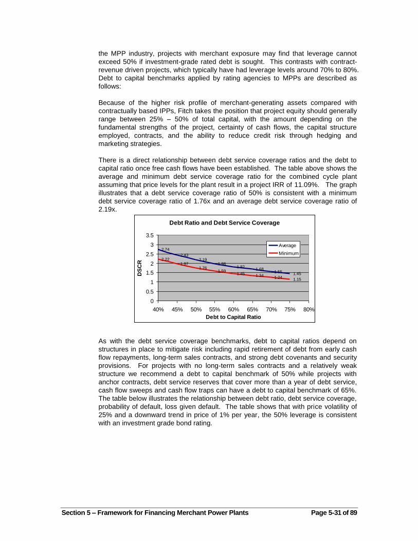
Section 5 – Framework for Financing Merchant Power Plants Page 5-31 of 89
the MPP industry, projects with merchant exposure may find that leverage cannot
exceed 50% if investment-grade rated debt is sought. This contrasts with contract-
revenue driven projects, which typically have had leverage levels around 70% to 80%.
Debt to capital benchmarks applied by rating agencies to MPPs are described as
follows:
Because of the higher risk profile of merchant-generating assets compared with
contractually based IPPs, Fitch takes the position that project equity should generally
range between 25% – 50% of total capital, with the amount depending on the
fundamental strengths of the project, certainty of cash flows, the capital structure
employed, contracts, and the ability to reduce credit risk through hedging and
marketing strategies.
There is a direct relationship between debt service coverage ratios and the debt to
capital ratio once free cash flows have been established. The table above shows the
average and minimum debt service coverage ratio for the combined cycle plant
assuming that price levels for the plant result in a project IRR of 11.09%. The graph
illustrates that a debt service coverage ratio of 50% is consistent with a minimum
debt service coverage ratio of 1.76x and an average debt service coverage ratio of
2.19x.
Debt Ratio and Debt Service Coverage
2.74
2.432.19
1.981.82
1.681.55 1.45
2.221.97
1.761.59
1.45 1.34 1.24 1.15
0
0.5
1
1.5
2
2.5
3
3.5
40% 45% 50% 55% 60% 65% 70% 75% 80%
Debt to Capital Ratio
DS
CR
Average
Minimum
As with the debt service coverage benchmarks, debt to capital ratios depend on
structures in place to mitigate risk including rapid retirement of debt from early cash
flow repayments, long-term sales contracts, and strong debt covenants and security
provisions. For projects with no long-term sales contracts and a relatively weak
structure we recommend a debt to capital benchmark of 50% while projects with
anchor contracts, debt service reserves that cover more than a year of debt service,
cash flow sweeps and cash flow traps can have a debt to capital benchmark of 65%.
The table below illustrates the relationship between debt ratio, debt service coverage,
probability of default, loss given default. The table shows that with price volatility of
25% and a downward trend in price of 1% per year, the 50% leverage is consistent
with an investment grade bond rating.

Section 5 – Framework for Financing Merchant Power Plants Page 5-32 of 89
5.7 Structural Enhancements to Mitigate the Credit Risk of MPPs
5.7.1 Introduction
The most important aspect of ADB’s underwriting process for an MPP will be
determining whether the plant is economically sound. This means that the cost
structure and the technology of the plant must be viable in relation to the existing
electricity system in the country. However, once a plant is determined to be
economically viable, the credit quality of a transaction can be enhanced by various
structural features. The potential for structural enhancements to improve the credit
quality of an MPP transaction is described in the statement by Standard and Poor’s
below:
Project structure does not mitigate risk that a marginally economic project presents to
lenders; structure in and of itself cannot elevate the debt rating of a fundamentally
weak project to investment-grade levels. On the other hand, more creditworthy MPPs
will feature covenants designed to identify changing market conditions and other risks
particular to MPPs and trigger cash trapping features to project lenders during
occasional stress periods.
Structural enhancements to the debt of an MPP can be classified into two general
ways. The first way to mitigate risk for debt holders is through financial
enhancements. This form of financial structuring which can take the form of financial
covenants, debt service reserves or subordinated debt to assure that the senior
lenders receive as much of the free cash flow as possible before equity holders take
out cash in the form of dividends. The second way to mitigate risk through structural
enhancements is to shift risk away from the MPP to other parties through bilateral
revenue and supply contracts. Some of the specific financial and contractual
enhancements which could be applicable to merchant plant financing include:
Financial Enhancements

Section 5 – Framework for Financing Merchant Power Plants Page 5-33 of 89
Cash flow capture covenants that cause debt to be re-paid early or debt
service reserves to be built-up if debt service coverage ratios are low.
Cash flow sweep covenants that cause debt to be re-paid early or debt
service reserves to be built-up if cash flow is high.
Debt service reserves that assure debt service can be paid if market prices
or other risks cause cash flow to be low for an extended period of time.
Subordinated debt and mezzanine finance that protects the cash flow
coverage of senior debt instruments.
Contingent equity or sponsor guarantees that provide for additional equity
funding in downside cases.
Contractual Enhancements
Bilateral vesting contracts with distribution companies during a transition
period.
Bilateral contracts with retailers or retail customers (tolling contracts are a
form of this structure).
Contracts with fuel suppliers and/or O&M contractors where operating
expense are subordinate to debt service.
Contracts with fuel suppliers where the price of fuel varies in when the
price of electricity varies.
Risk hedging through use of forward contracts.
Combination of MPPs in to portfolios to moderate asset concentration.
The manner in which these structural enhancements should impact the ADB’s
process of underwriting debt for an MPP transaction is described below. In assessing
whether to include various enhancements in a transaction and how to price
transactions with and without various enhancements, the ADB must be able to value
the different structural elements. To value of the different enhancements we evaluate
how the financial and contractual mechanisms affect the probability of default and the
loss given default of a loan. We begin by measuring the value of financial
enhancements and then we describe how to value contractual enhancements.
5.7.2 Financial Enhancements and Financial Structuring
Typical MPP transactions allow at some level of dividends to be paid to sponsors
from cash flow before all of the debt has been repaid. Furthermore, project financings
often have various tranches of debt where cash flow is not applied to subordinated
debt unless all of the senior debt service is paid. Various structural techniques can be
used to protect the position of senior debt holders relative to other investors including
covenants that restrict dividend payments, debt service reserve accounts and inter-
creditor agreements between senior and subordinated debt. In developing a debt
structure for an MPP, the ADB must assess which type of covenant is most important
and whether structuring elements such as cash flow traps are more important than
large debt service reserves. Furthermore, if the ADB takes a subordinated position to
senior debt, the pricing of the subordinated debt issue relative to the senior debt must
be established.
5.7.3 Covenants
Loans typically include a set of positive and negative covenants. Positive covenants
include terms such as having business insurance, having audited accounts and
keeping equipment in good condition. Negative covenants generally include

Section 5 – Framework for Financing Merchant Power Plants Page 5-34 of 89
limitations on risky business activities and limitations on issuing additional debt. In
addition to typical covenants, an MPP transaction can include controls on cash flows
that limit the amount of dividends that can be paid to sponsors. The limitations on
cash flows are designed with the debt service coverage ratio.
Covenants can restrict the amount of dividends paid to sponsors during good time
and bad time periods. Covenants that restrict cash flow in bad time periods are
known as cash traps. Covenants that limit cash payments when cash flow is high are
known as cash flow sweeps. These covenants are explained as follows by Standard
and Poor’s:
Standard & Poor’s believes that a project’s credit is generally strengthened by
covenants that limit, or even preclude, distributions to sponsors unless both robust
historic and projected DSCRs are met, and reserve funds are fully funded.
The reason for dividend restrictions in time periods when cash flow is low is because
when financial results are worse than expected, it is essential to assure that cash
flow is kept for the debt holders and not ―leaked‖ out of the project as dividends. A
cash flow trap operates by limiting any dividend payments if the debt service
coverage is below a debt service ratio criteria. If the dividend restriction is tied to a
relatively high level of the debt service coverage such as 2.5x, the dividend restriction
will occur more often than if the dividend restriction is set to a relatively low level such
as 1.2x – the ―bad‖ time periods occur more often with the higher covenant. Since the
covenant limits dividends, cash flow traps mean that something must be done with
the cash flow that is not distributed to sponsors. Cash either can be used to payoff
debt early or be put into a debt service reserve to protect debt holders.
The graphs below show how cash flow traps affect cash flows to equity and debt
holders. The first graph illustrates cash flow in a situation without price volatility
where the spot price follows a downward trend. The bars on the graph represent total
cash flow to the MPP project and cash flow received or distributed by equity holders.
The second graph shows the cash flows in a situation where prices vary from year to
year due to assumed price volatility. In the second graph dividends are paid to
shareholders in early years when electricity prices are relatively high while dividends
cannot be paid in later years when prices are lower.
Cash Flow
(30,000.00)
(25,000.00)
(20,000.00)
(15,000.00)
(10,000.00)
(5,000.00)
-
5,000.00
10,000.00
15,000.00
20
00
20
01
20
02
20
03
20
04
20
05
20
06
20
07
20
08
20
09
20
10
20
11
20
12
20
13
20
14
20
15
20
16
20
17
20
18
20
19
20
20
20
21
20
22
20
23
20
24
20
25
20
26
20
27
20
28
20
29
Equity Cash Flow
Free Cash Flow

Section 5 – Framework for Financing Merchant Power Plants Page 5-35 of 89
Cash Flow
(30,000.00)
(25,000.00)
(20,000.00)
(15,000.00)
(10,000.00)
(5,000.00)
-
5,000.00
10,000.00
15,000.00
20,000.00
25,000.00
20
00
20
01
20
02
20
03
20
04
20
05
20
06
20
07
20
08
20
09
20
10
20
11
20
12
20
13
20
14
20
15
20
16
20
17
20
18
20
19
20
20
20
21
20
22
20
23
20
24
20
25
20
26
20
27
20
28
20
29
Equity Cash Flow
Free Cash Flow
In the scenario with price volatility, the debt cannot be repaid as cash flows are lower
in the ending year of the project. Debt is scheduled to be re-paid in these latter years,
but it cannot be fully re-paid as shown in the graph below. The graphs imply that
dividends were paid to shareholders even though the total debt could not be repaid.
2005 2009 2013 2017 2021 2025 2029
-
5,000.00
10,000.00
15,000.00
20,000.00
25,000.00
30,000.00
35,000.00
40,000.00
45,000.00
50,000.00
Ending Debt
Senior Debt First Juinor Tranche
Second Junior Tranche Third Junior Tranche
With a covenant that ―traps‖ cash flow and restricts dividends unless the debt service
coverage is above 2.0x, the dividends are limited as shown in the graph below. The
covenant simply means that any time the debt service coverage is below 2.0x, no
dividends can be paid. In years when the cash flow is relatively low – three of the
years on the graph below – dividends are not allowed to be paid to shareholders
because of the covenant. The cash that would have been paid as dividends is used
to re-pay debt early and there is less debt to re-pay at the end of the project life. This
limitation on dividends means that the total amount of the debt can be repaid.
Cash Flow
(30,000.00)
(25,000.00)
(20,000.00)
(15,000.00)
(10,000.00)
(5,000.00)
-
5,000.00
10,000.00
15,000.00
20,000.00
25,000.00
20
00
200
1
20
02
20
03
20
04
20
05
200
6
20
07
20
08
20
09
20
10
20
11
20
12
201
3
20
14
20
15
201
6
20
17
20
18
20
19
20
20
202
1
20
22
20
23
202
4
20
25
202
6
20
27
20
28
20
29
Equity Cash Flow
Free Cash Flow

Section 5 – Framework for Financing Merchant Power Plants Page 5-36 of 89
If the cash flow trap is more restrictive – the covenant is set to a higher level -- the
debt should experience a lower probability of default. A more restrictive covenant
implies a lower probability of default. This should also imply that a lower credit spread
can be accepted in the pricing of debt. Probability of default and loss given default
can be measured by including the cash trap in the project finance model and
applying the Monte Carlo simulation with alternative levels of cash trap covenant
restrictions. The table below presents the probability of default, the loss given default
and the required credit spread for different levels of cash trap covenants assuming
price volatility of 25% and debt leverage of 60%. The table demonstrates that if the
dividend is restrictive in the sense that dividends are rarely allowed until all of the
debt is repaid, the credit spread falls by almost 300 basis points. The reason the
probability of default declines by such a large amount is because the highly restrictive
covenant essentially means that all debt is repaid before any dividends are allowed.
A second type of covenant applies in periods when cash flow is high rather than
when cash flow is low. The reason for restrictions on dividends in good time periods
is because when prices higher than normal, cash flow can be kept for the debt
holders to protect against default in later periods when cash flow and prices may be
below normal. Cash flow sweeps operate by computing the amount of dividends that
will just limit the debt service coverage to the covenant. Unlike the cash traps, if the
cash sweep covenant is set to a low level it is more restrictive (the cash flow trap
covenant described above was more restrictive with a higher level). If the cash sweep
is tied to a relatively low level of the debt service coverage such as 1.5x, the dividend
restriction will occur more often than if the dividend restriction is set to a relatively low
level such as 3.5x. The graph below uses the volatile price scenario presented above
to illustrate how dividend payments are reduced in a scenario with a covenant that
sweeps cash flow. In the scenario with cash flow sweeps, no dividend payments are
allowed in the early years until much of the debt is paid off. As with the dividend
restriction the covenant, the cash flow sweep allows the debt to be fully paid off
because dividends are not ―leaked‖ out of the project to shareholders.
Cash Flow
(30,000.00)
(25,000.00)
(20,000.00)
(15,000.00)
(10,000.00)
(5,000.00)
-
5,000.00
10,000.00
15,000.00
20,000.00
25,000.00
20
00
20
01
20
02
20
03
20
04
20
05
20
06
20
07
20
08
20
09
20
10
20
11
20
12
20
13
20
14
20
15
20
16
20
17
20
18
20
19
20
20
20
21
20
22
20
23
20
24
20
25
20
26
20
27
20
28
20
29
Equity Cash Flow
Free Cash Flow
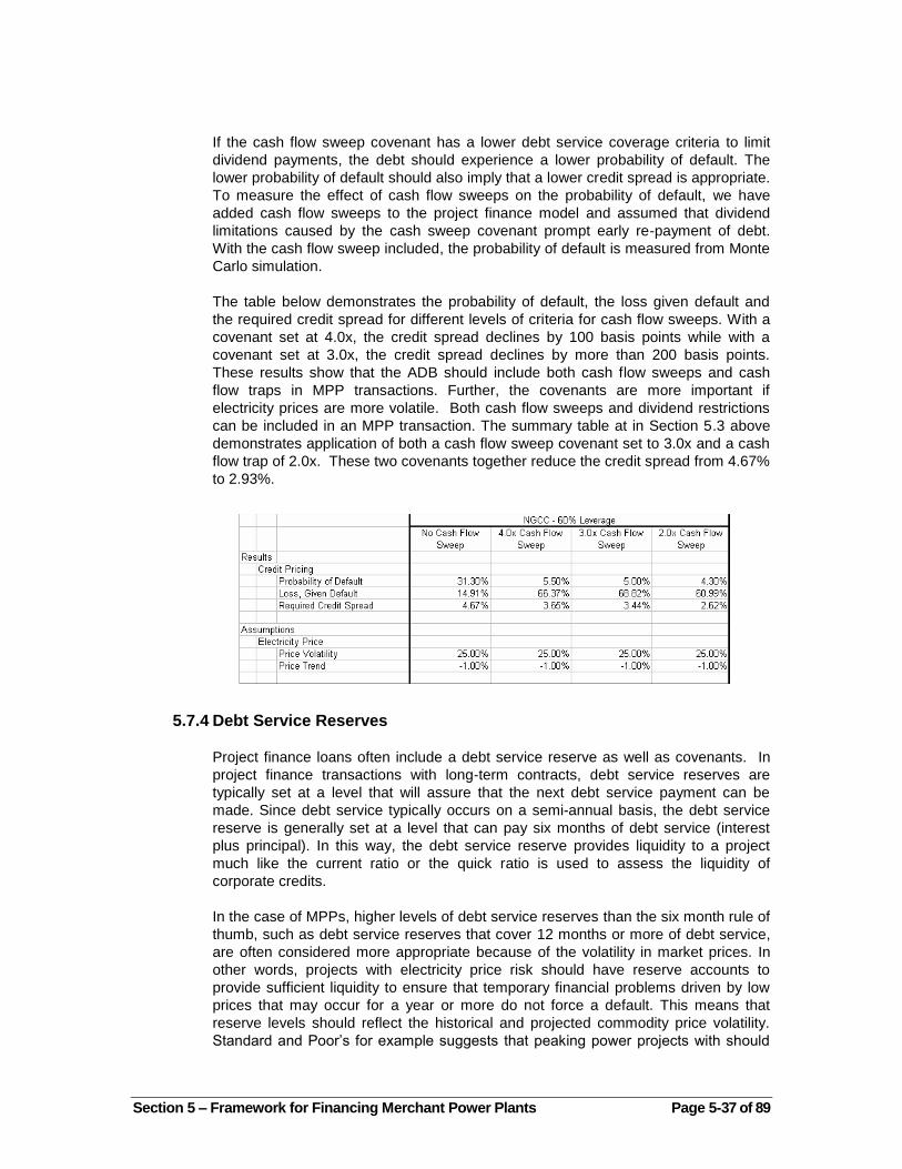
Section 5 – Framework for Financing Merchant Power Plants Page 5-37 of 89
If the cash flow sweep covenant has a lower debt service coverage criteria to limit
dividend payments, the debt should experience a lower probability of default. The
lower probability of default should also imply that a lower credit spread is appropriate.
To measure the effect of cash flow sweeps on the probability of default, we have
added cash flow sweeps to the project finance model and assumed that dividend
limitations caused by the cash sweep covenant prompt early re-payment of debt.
With the cash flow sweep included, the probability of default is measured from Monte
Carlo simulation.
The table below demonstrates the probability of default, the loss given default and
the required credit spread for different levels of criteria for cash flow sweeps. With a
covenant set at 4.0x, the credit spread declines by 100 basis points while with a
covenant set at 3.0x, the credit spread declines by more than 200 basis points.
These results show that the ADB should include both cash flow sweeps and cash
flow traps in MPP transactions. Further, the covenants are more important if
electricity prices are more volatile. Both cash flow sweeps and dividend restrictions
can be included in an MPP transaction. The summary table at in Section 5.3 above
demonstrates application of both a cash flow sweep covenant set to 3.0x and a cash
flow trap of 2.0x. These two covenants together reduce the credit spread from 4.67%
to 2.93%.
5.7.4 Debt Service Reserves
Project finance loans often include a debt service reserve as well as covenants. In
project finance transactions with long-term contracts, debt service reserves are
typically set at a level that will assure that the next debt service payment can be
made. Since debt service typically occurs on a semi-annual basis, the debt service
reserve is generally set at a level that can pay six months of debt service (interest
plus principal). In this way, the debt service reserve provides liquidity to a project
much like the current ratio or the quick ratio is used to assess the liquidity of
corporate credits.
In the case of MPPs, higher levels of debt service reserves than the six month rule of
thumb, such as debt service reserves that cover 12 months or more of debt service,
are often considered more appropriate because of the volatility in market prices. In
other words, projects with electricity price risk should have reserve accounts to
provide sufficient liquidity to ensure that temporary financial problems driven by low
prices that may occur for a year or more do not force a default. This means that
reserve levels should reflect the historical and projected commodity price volatility.
Standard and Poor’s for example suggests that peaking power projects with should

Section 5 – Framework for Financing Merchant Power Plants Page 5-38 of 89
have 12 to 18 months' debt service reserve funds. While debt service reserves
protect the position of lenders, the debt service reserves are expensive from the
perspective of sponsors because more capital must be raised for the project and
because the interest rate earned on funds in a debt service reserve is very low
compared to the expected return earned on the project.
The graph below illustrates how a debt service reserve can protect lenders to an
MPP project. With a high level of a debt reserve, when cash flow is insufficient to pay
debt service, the cash flow is used to put money back into the debt service reserve.
If the debt service reserve has been used to pay meet debt service obligations in an
earlier year and it is not at its required level, the debt service reserve must be
replenished before debt can be repaid. This means that when cash flow is positive,
cash must be used to replenish the reserve instead of flowing to equity holders as
dividends. In the scenario used to develop the graph, without the debt service
reserve, the cash flow would not have been sufficient to pay off the debt. With the
debt service reserve, the debt can be fully repaid.
5.7.5 Senior and Subordinated Debt
An important ADB product in assisting the development of MPPs in Asia may be
subordinated debt or junior debt offerings that have a longer term than senior debt.
With subordinated debt in the capital structure of an MPP, the cash flow first pays all
of the debt service on a senior debt issue and only the remainder is used for junior
debt. Because use of subordinated debt in an MPP capital structure means that
senior debt service is lowered, the existence of subordinated debt improves the credit
quality of the senior debt. Given the reluctance of financial institutions to finance MPP
debt after financial problems that have occurred in the industry, ADB subordinated
debt issued for an MPP project could be the difference between projects being
developed and not being developed. From the perspective of senior debt holders, a
subordinated debt strategy may partially mitigate commodity electricity market risk,
either initially or after a bilateral contract expires when a project faces electricity price
market risk. If subordinated debt is used in an MPP transaction, an inter-creditor
agreement must be established that carefully defines restrictions on the payment of
subordinated debt service to protect the senior debt holders. Use of subordinated
debt is illustrated in the table below. Note that the senior debt service coverage
improves while the junior debt service coverage is lower than the senior debt service
coverage.

Section 5 – Framework for Financing Merchant Power Plants Page 5-39 of 89
If the ADB finances subordinated debt it will not be able to require payment without
prior senior debt holder approval. Such debt must be deeply subordinated to senior
debt with severely limited rights of acceleration or access to project collateral.
Repayment of such subordinated debt should be well below other cash claims, falling
just ahead of equity dividends. While subordinated debt can support MPP
development, underwriting subordinated debt and establishing the credit spread for
subordinated debt is a complex process.
The pricing of subordinated debt can be assessed in a similar manner as the process
described above for a single debt issue. To measure the probability of default and the
loss given default for subordinated debt, the project finance model is structured with a
cash flow waterfall to measure the amount of subordinated debt and senior debt that
remains at the end of the life of the project. Once the project finance model includes
a cash flow waterfall, the probability of loss and the loss given default can be
assessed with Monte Carlo simulation. The table below illustrates the required credit
spread, the probability of loss and the loss given default for both senior and
subordinated debt assuming different levels of senior and junior debt. We present two
scenarios with junior debt – one with a junior debt issue that comprises 30% of the
total debt and another where the junior debt issue is 50% of the total debt. In all
cases, the total senior and junior debt together represents 60% of the total cost of the
project. The table demonstrates that use of junior debt dramatically reduces the risk
of the senior debt – to the point at which if 50% of the debt is subordinated, the
required credit spread for senior debt is below .5%. Of course, the required credit
spread and the risk of the junior debt exceeds the credit spread of the senior debt.
The analysis of subordinated debt in the table below demonstrates that the ADB can
use junior debt as a tool to attract capital to an MPP. However, if the ADB uses junior
debt as a tool, the pricing must reflect the additional risk.
Section 5 – Framework for Financing Merchant Power Plants Page 5-40 of 89
The above analysis of covenants, debt service reserves and subordinated debt
illustrates that the process for evaluating financial enhancements that mitigate or
allocate risk is complex. The risks can be gauged using a mathematical process that
incorporates the volatility of electricity prices. However, even if the mathematical
techniques are not applied in practice, the conceptual points demonstrated by use of
the complex approach should be included by the ADB in its credit analysis process to
underwrite MPP transactions.
5.7.6 Contractual Enhancements and MPP Credit Analysis
The financial structuring enhancements discussed above can mitigate risk by
allocating cash flow available to the MPP to various classes of debt and equity
investors. In addition to covenants, debt service reserves and subordinated debt,
contractual enhancements such as bilateral contracts can mitigate MPP risk. Unlike
the case of covenants, debt service reserves and subordinated debt, risk is not
simply allocated between equity holders and debt holders. Instead, in the case of
using contracts to mitigate risk, cash flow risk is allocated to parties who do not invest
in the MPP. The most commonly discussed way to mitigate risk through contracts is
through bilateral long-term contracts with power purchasers. Other ways to use
contracts to mitigate risk of an MPP include supply contracts that are subordinate to
debt service, supply contracts structured so the fuel price varies when the electricity
price varies and use of forward markets to mitigate revenue risk.
The remainder of this section describes how the various contractual enhancements
affect the underwriting of ADB debt and the credit spread that is appropriate for MPP
transactions. We begin by assessing how bilateral purchase contracts affect risk and
then move to supply contracts and risk hedging. The process of valuing the credit
aspects of the contractual enhancements applies the probability of default and the
loss given default approach discussed above.
5.7.7 Risk Mitigation with Bilateral Revenue Contracts
An MPP was defined in Part 1 as a plant that can have a bilateral contract. The plant
was defined as an MPP as long as the contract between the MPP and the off-taker is
subject to commercial risk. This means that a plant which signs a contract with a
retail customer who can purchase from the market; a plant that signs a contract with
a retailer subject to market competition in dealing with retail customers; a plant that
signs a contract with a marketer who sells power in wholesale markets using a tolling
agreement; or a plant that signs a contract with a distributor that is subject to retail
choice are all defined as merchant plants. Finally, a plant that signs a vesting
contract with a distribution company which is government owned or government
regulated and has non-contestable customers is considered a hybrid MPP.
This section discusses how bilateral contracts can mitigate risk of ADB MPP
transactions. We first describe the nature of bilateral contracts and then discuss how
these contracts affect the ADB underwriting process and the pricing of ADB debt
instruments. In addition to mitigating risks for individual MPP transactions, bilateral
contracts raise a number of important policy issues in the context of developing a
market framework. Bilateral contracts can lower the cost of capital to MPPs and
moderate price volatility in a market. However, vesting bilateral contracts can also
defeat some incentives to purchase and supply electric power in an economically
efficient manner. Quantification of these policy issues associated with bilateral

Section 5 – Framework for Financing Merchant Power Plants Page 5-41 of 89
contracts including the cost of capital are addressed in Section 5.8 below.
Until recently, MPPs that sold power much of their power at spot market prices were
considered more attractive than plants that had all of their power sold under bilateral
contracts. For example, MPPs in the US often received commitments for only 40-65
percent of their power sales. The idea was that the remainder of the power would be
sold at market rates and receive higher spot market prices. The notion of receiving
higher profit from selling spot power fell apart in the US as natural gas prices
increased and as wholesale electricity prices fell because of declines in demand and
too much generation supply. Given changes in the market, merchant companies that
attempted to sell significant power at spot prices have realized profit margins which
are so thin that many have had trouble covering their fixed costs.
If an MPP has a bilateral contact such as a tolling agreement or a long-term contract
for difference with a retailer, market risks can be mitigated and higher debt leverage
can be obtained. In terms of risk allocation, bilateral contracts are similar to power
purchase agreements in that they provide a stable stream of cash flow in the form of
contractually based revenues. In some cases the risks that remain with the MPP after
signing a bilateral contract with a marketer or with a retailer are less severe than
those remaining under a power purchase agreement with a utility. For example,
typical tolling arrangements imply that the risks assumed by the MPP sponsor are
limited only to the availability of the plant and the plant efficiency.
In underwriting transactions that include bilateral contracts, the ADB must assess the
market price risks that remain once the bilateral transaction expires and the risks that
the counterparty to the bilateral contact will not be able to meet obligations of the
contract. The creditworthiness of utility company off takers can generally be captured
in the utility's corporate credit rating. In traditional IPP/PPA transactions the bond
rating of the off taker often did not cause problems in terms of underwriting the loans.
For example, because the average utility rating was often in the A category, the
project debt was typically rated BBB. On the other hand, off takers for MPPs are
generally retail customers, retailers, or energy marketing and trading companies.
These companies either have lower credit rating or do not have a credit rating. To
compound the problem, off takers will be most likely to default when the bilateral
contract is out of the market and the MPP will not be able to make up lost revenues
from the contract through making spot market sales. The case study of AES Drax
discussed in Part 3 highlights this problem.
To quantify the effect of bilateral contracts for purposes of underwriting and
determining credit spreads, we describe two approaches below. The first method
involves break-even analysis to determine the minimum price at which power can be
sold and debt can be serviced. This break-even technique can establish the level of
market prices for different amounts of debt leverage and different bilateral contract
terms. The second method applies the Monte Carlo simulation technique to measure
the probability of loss and the loss given default assuming different bilateral contract
terms. This method can incorporate the credit quality of off-takers as well as the
volatility of market prices.
The break-even approach is illustrated for evaluating the risk mitigating effects of
bilateral contracts is shown in the series of tables below. These tables present the
break-even price for different assumed leverage levels and for different contract
assumptions. Pricing in the contract is driven by assuming the contract price is
$4/MWH below the expected spot price. We apply three different assumptions with
respect to contract levels in the case study. The first scenario assumes no contracts,

Section 5 – Framework for Financing Merchant Power Plants Page 5-42 of 89
the second scenario assumes 50% of the plant is contracted for 7 years and the third
scenario assumes 100% of the power is contracted for 10 years. For each of the
contract scenarios, we measure the lowest amount the market price can be and still
meet debt service obligations.
The ability to meet debt service obligations using break-even prices is measured
using two alternative approaches. The first approach measures the break-even price
by determining how low the market price can be and still maintain a minimum debt
service coverage above 1.0. The second approach measures the minimum market
price that can be achieved and assure that no debt is outstanding at the end of the
life of the project. The break-even analysis is shown for the NGCC plant, the coal
plant and the CT plant in the three tables below. The table shows that the coal plant
has the most margin for a lower price because its capital base – the debt service and
dividends are higher than for the less capital intensive plants. The tables also
illustrate how contracts equate to a higher level of leverage. For a certain acceptable
break-even price, the risks can be mitigated either through a contract or through
lower levels of leverage. In the case of an NGCC plant, a level of leverage of 45%
with no contact is approximately the same as 75% leverage with a 10 year bilateral
contract. The analysis makes it clear that ADB products which support contracts such
as risk insurance on the contract are important from the perspective of MPP
developers.
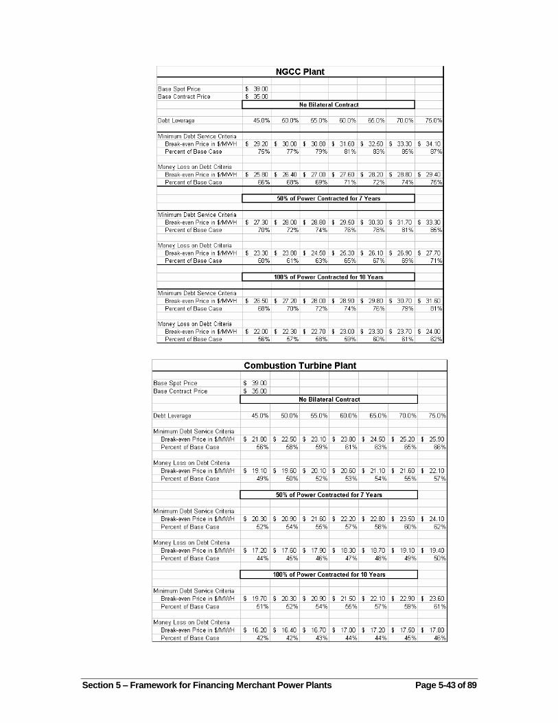
Section 5 – Framework for Financing Merchant Power Plants Page 5-43 of 89

Section 5 – Framework for Financing Merchant Power Plants Page 5-44 of 89
The Monte Carlo simulation approach for evaluating the risk effects of bilateral
contracts is shown in the table below where the probability of loss and the loss given
default is applied to different bilateral contract assumptions. In this analysis, three
different contract cases are assumed. Unlike the break-even analysis, the Monte
Carlo approach can be used to directly assess how the bilateral contract affects
required credit spreads. The approach can also incorporate the probability of default
inherent in the power contract. In the table below, the contract is assumed to default
10% of the time if the market price is below the contract level.
Data in the table demonstrates the importance of bilateral contracts to the
underwriting process of an MPP. With a 5 year contract that only covers 50% of the
generation of an MPP the required credit spread is reduced by almost 250 basis
points. With a 10 year contract that covers all of the plant output, the credit spread
declines to only .76%. These risks are reduced despite lower returns for the project
that result from the contract price being below the expected spot price. The credit
benefits of bilateral contracts shown in the table below demonstrate that ADB
facilitation of bilateral contracts can be instrumental in development of the MPP
industry.
5.7.8 Risk Absorption from Suppliers
Power plants that had long-term contracts fixed the level of revenue and many other
items. If revenues are fixed, then operating and maintenance costs, fuel expenses,
interest expenses and other items should also be fixed. In the case of an MPP,
revenue is not fixed, and cash flow risk can be moderated if expenses vary in the
same direction as revenues. For example if fuel expense declines when prices
decline, cash flow risk will be reduced. An example of costs varying in the same
direction as revenues is Fuel Supply subordination. The fuel subordination in an MPP
can take various forms. In the extreme, fuel is supplied to the plant at no cost when
the electricity price is low. In less extreme cases, the price of fuel is reduced when
the electricity price is low.
The following quote from Fitch Investor Services illustrates fuel subordination for a
gas-fired merchant plant in the Northeast US (the Digton Power Plant):
A significant credit factor in the transaction is the enhancement offered by the
Section 5 – Framework for Financing Merchant Power Plants Page 5-45 of 89
subordination of the natural gas commodity costs to the senior debt service
payments. As part of the long-term fuel supply arrangement with an investment-
grade supplier, the supplier was willing to subordinate moneys received to non-
fuel operating expenses, reserves, and senior debt service over the life of the
bonds. This subordination constitutes a form of quasi-equity.
In MPP transactions involving fuel intensive plants such as oil plants or gas plants,
the use of fuel supply contracts that moderate risk is equivalent to the lower price
volatility. The ADB should encourage the use of fuel subordination agreements in
underwriting credit and should facilitate the contracts by offering insurance for the
contracts.
5.7.9 Hedging of Market Risks through Forward Contracts
As stated in Part 3 of the report, one of the most important aspects of developing a
market framework is assuring that a forward market exists by which prices can be
hedged. With liquid forward markets, it is possible to hedge both the price and the
volume of dispatch risk of MPPs. The manner in which risks can be hedged using
forward markets is illustrated by considering a natural gas combined cycle plant.
Through use of options markets for both natural gas and electricity, the price and
volume risks can be fully hedged. Assume the gas price is $3/MMBTU and the heat
rate is 10,000 BTU/kWh and there is no variable O&M expense then the variable cost
of the plant is $30/MWH. When the electricity price is above $30/MWH the plant is
dispatched and a margin of the electricity price minus $30/MWH is earned. The plant
earns cash flows if the electricity price is above $30/MWH and it makes cash outflows
to pay for the cost of gas. A series of option contracts on natural gas prices and
electricity prices can be structured to fully hedge both the volume and price risk of the
plant. The problem with this type of hedging strategy is that forward contracts do not
exist for terms that correspond to debt tenors. Therefore, the remaining merchant
must be established in a similar manner to the contract case discussed above.
Appendix 5 addresses some technical aspects of hedging the risk of MPPs.
5.8 Analytical Models to Evaluate Policy Issues Associated with Market
Frameworks
5.8.1 Analytical Models and ADB Strategy Reports
The ADB Staff formulates five year strategies for reform of sectors in developing
nations that encourage sustainable and efficient development. These strategic plans
include a ―wish list‖ for what the country should do in the generation sector regarding
transparent contracting, efficient pricing, encouraging reliable supply, limiting
monopolist behaviour by private developers and other policies that promote
sustainable development. One of the reasons for developing the roadmap for a
market framework described in Section 5.1 was to guide the ADB Staff in developing
these strategic reports. Many of the recommendations included in the above
roadmap describe essential elements of a market framework that clearly should be
put in place to support MPP development. For example, we recommended that
distribution, generation and transmission should be unbundled; that market
mechanisms must be established with equal access to transmission; that privatisation
should not create market power; that spot prices should be published, and that
forward markets should be established which allow merchant plants to hedge market

Section 5 – Framework for Financing Merchant Power Plants Page 5-46 of 89
risks. These recommendations are ―home truths‖ that need not be analysed or
quantified with modelling analysis.
Another set of recommendations relates to open issues involving market
implementation and the required MPP framework. These issues include:
1) do the benefits from bilateral contracts from the standpoint of attracting
merchant capacity off-set the costs of bilateral contracts on optimal market
behaviour;
2) do the benefits of price caps in terms of limiting market power offset
economic distortions in the market;
3) do the benefits of a cost-based energy market in terms of limiting market
power offset the lack of economic incentives and the administrative capacity
price mechanisms that are required in a cost based system; and
4) what type of capacity pricing system should be implemented to attract
merchant capacity and limit the exercise of market power.
Price forecasts using simulation models are presented below to evaluate impacts of
policy alternatives available to developing countries and risks faced by the ADB as an
investor in merchant power plants. For example, price forecasts using forward price
simulation models evaluate how various capacity pricing structures affect long-term
price levels, price volatility, the reliability of electricity supply, and the amount and mix
of capacity in the long-term. To analyse policy with respect to a capacity pricing
framework, we have used a common set of assumptions with respect to loads, the
cost of new capacity, fuel prices and other variables. The analyses presented below
are evaluated assuming different policies with respect to price caps, different
administrative determinations of reserve margin, value of lost load (―VOLL‖), and
different behaviour of private developers.
5.8.2 Use of Forward Price Simulation Models to Evaluate Policy Issues
Long-term forward price models introduced above in Section 5.4 can be used to
evaluate whether policies included in a market framework will be beneficial for people
and businesses of developing countries as well as to support MPP investment
analysis. To illustrate how modelling can be used in policy analysis, consider how a
developing country should decide upon the best design of a market structure for
capacity prices. As discussed in Part 3, alternative market designs with respect to
capacity pricing include:
1) Bid-based systems with an energy only price and no price caps or price caps
sufficiently high to support peaking and reserve capacity, such as the systems used in Australia and Nordpool;
2) Separate installed capacity markets that have been implemented in PJM and
the New York Pool in the US;
3) Administratively determined capacity support such as the method used in
South Korea and Columbia; and
4) Application of a uplift to energy prices such as adding the value of lost load
(―VOLL‖) to energy charges that is dependent on loss of load probability

Section 5 – Framework for Financing Merchant Power Plants Page 5-47 of 89
(―LOLP‖) such as the market originally used in the UK and the system in place
in Argentina.
In assessing which market design is best for a particular country, policy makers must
address a number of issues in deciding on the appropriate market structure. Four
issues include assuring that markets will: (1) provide reliable electricity to consumers;
(2) be sustainable in the long-run through attracting capacity from private developers;
(3) result in prices that are not extremely volatile; and, (4) minimize the potential of
generating companies to exercise market power.
To illustrate how analytical models can be used to evaluate tradeoffs inherent in
various policy questions, the table below summarizes customer costs in a simulation
model using different scenarios with respect to capacity pricing and market power.
The details of various numbers in the table are presented in the paragraphs below.
The measurement uses index numbers where geared to an ideal perfect market with
no market power and no government interference. The first row shows customer
costs that would occur in a pure optimal scenario without market power and with an
ideal bid-based capacity pricing system. The second and third rows show the
increased prices that can result from exercise of market power at times of high prices.
These rows illustrate that the ideals of a market system can be evaporated if private
companies can exercise market power. The fourth and fifth rows illustrate the effects
of different levels of price caps – a cap of $1,500/MWH and $300/MWH --
implemented to moderate market power. The analysis depends on many
assumptions and analytical techniques that are described below in Section 5.9.
The above table does not answer the question of whether price caps should be put in
place to address market power considerations. Rather, the analysis illustrates how
the ADB can use technical assistance tools presented in this part of the report to
illustrate the possible impacts and tradeoffs inherent in alternative policy options.
The implication of the above table is that the ADB can perform analyses that quantify
the effects of different market designs.
5.8.3 Policy Analysis, MPP Cost of Capital and Bilateral Contracts
Part 3 of the MPP report described how policies implemented in creating a framework
for market generation can affect the willingness of MPPs to make investments in a
country. The manner in which a framework affects promotion of MPPs can be
quantified in terms of the cost of capital and the carrying charge. As described in Part
3 of the MPP report, there has been a major change in the attitude of financiers to

Section 5 – Framework for Financing Merchant Power Plants Page 5-48 of 89
MPP investments that make financing new MPPs more difficult. The increased
difficulty in obtaining financing is quantified below by measuring the cost of capital
before and after the ―financial meltdown.‖
The relationship between cost of capital and debt structure can be illustrated by
considering a hypothetical decision making process in the financial analysis
department of an energy company. Begin with the notion that management has a
rate of return criteria where only projects that have an IRR of above 14% are
approved for investment and projects that have an IRR below 14% are not. Further,
assume that this rate of return is measured using equity cash flow rather than free
cash flow, due to corporate objectives related to earnings per share (―EPS‖) growth.
In this hypothetical situation as long as free cash flow from the project is expected to
yield a higher rate of return (project IRR) than the after tax cost of debt, the equity
return can be increased if more debt is used to finance the asset. (Magnifying asset
returns to increase equity return is the where the term leverage comes from). If,
because of the reluctance of bankers to take credit risk, debt cannot be raised for the
project, the equity return criteria will probably not be met. On the other hand, if a
significant amount of project debt can be raised, the equity IRR will exceed 14% and
the investment will be made. Therefore, in this hypothetical example the amount of
debt directly affects the investment decision. Indeed, the investment is driven by the
amount of debt that can be raised rather than by the beta of the project or the risk
adjusted all-equity cost of capital relative to the project IRR.
The notion that the leverage of a project affects cost of capital is demonstrated in the
following quote from a rating agency:
Nonetheless, a project's leverage level is often an indication of its
creditworthiness. For instance, a merchant project's ability to produce a stable
and predictable revenue stream will never match that of a traditional contract
revenue-driven project. Projects with merchant exposure may find that leverage
cannot exceed 50% if investment-grade rated debt is sought. Contract-revenue
driven projects, on the other hand, typically have had leverage levels around
70% to 80%.
5.8.4 Policy Analysis, MPP Cost of Capital and Bilateral Contracts
This section describes how the environment surrounding a market framework affects
the cost of capital, the carrying charges and the investment activity of merchant plant
developers. The carrying charge for a merchant plant which includes required equity
returns, debt service payments and income taxes affects the long-run marginal cost
and the forward pricing models. Carrying charges therefore can be used to quantify
how policies that change the cost of capital affect electricity prices required before
investors will install capacity.
Measurement of the cost of capital and carrying charges can be used to quantify how
policy alternatives that encourage MPP development such as promoting bilateral
contracts and assuring financially stable off-takers affect the cost of electricity to
consumers. Bilateral contracts lower the cost of capital for merchant plants and
should attract more capacity and lower electricity prices. To demonstrate how cost of
capital is affected by the financial and market environment we quantify how changes
in the cost of capital impacts electricity prices.
The analysis below illustrates how changes in the ability of merchant developers to
Section 5 – Framework for Financing Merchant Power Plants Page 5-49 of 89
raise money affect consumer costs in a competitive market. To illustrate this, three
scenarios are developed to represent financing conditions facing merchant
developers in the recent past. The first case applies aggressive financing that
occurred in the UK in the late 1990’s. Many of these plants were able to realize debt
to capital ratios of more than 80% with debt tenors exceeding 20 years and with
interest rates of about 1.5% above the LIBOR rate. We assume that investors that
investors require a 15% equity return (the equity IRR) in order to make an investment.
These financing characteristics are applied to the combined cycle and the coal plant
characteristics described in Section 5.3.
The second case applies a more typical merchant financing which assumes a debt to
capital ratio of 60%, a debt tenor of 15 years and an interest rate spread of 2.0%.
This case also assumes a required rate of return of 16%. This financial structure is
typical of merchant plants that have been financed in the past.
The financing structure applied to merchant power development in the 1990s is
generally considered to be too aggressive relative to risks that are inherent with
competitive electricity. For example, in the US, private companies that own merchant
plants have lost of more than $100 billion in market capitalization since 2002. In 2003,
three very large companies in the merchant power industry -- NRG Energy, Mirant
and Pacific Gas & Electric's unregulated generation subsidiary -- filed for bankruptcy.
Because of these financial failures there is a consensus that future financing will be
far more conservative. Four examples of recent commentary by financiers are listed
below:
―While competitive power fundamentals may never point to great
business, firms in other industries can survive under similar
circumstances and may even do well, but they do so under much
more conservatively financed structures than many energy
merchants first envisioned,‖
Banks are ―now highly reluctant to take merchant risk of any kind…
and they are sceptical about long-term purchase or tolling contracts
that in any are considered to be out of the money.‖
Merchant risk is usually BB risk – junk bond status -- at most unless
it benefits from a very conservative finance structure.
Merchants will have to redesign their business models. Those
players that have 80-90 percent of their capital in the form of debt
won't survive. The ratings agencies have said that such debt-to-
capital ratios must be in the 50-50 range to earn investment grade
status so that the cost of borrowing is reasonable.
To model the impacts of a conservative capital structure, we assume a 50-50 capital
structure, a debt tenor of 10 years and a credit spread reflective of below investment
grade bonds of 3.5%. Given the problems with losses on plants, we assume that
investors in the future require a 17% equity return. As compared to the aggressive
financing realized in the past, investors would have to expect higher electricity prices
before making an investment with this financing structure.
The two tables below illustrate how differences in the financial structure of MPPs
affect the average annual price required for an MPP plant. The first table shows

Section 5 – Framework for Financing Merchant Power Plants Page 5-50 of 89
results for the combined cycle plant and the second table shows results for the coal
plant. The tables demonstrate how an aggressive financing structure representative
of UK MPPs results in a required market price of $29/MWH for the combined cycle
plant while the typical MPP financing structure prior to the financial meltdown results
in a price of $32/MWH. The conservative financing structure reflective of current
conditions results in a price of $35/MWH. This means that the worse conditions
surrounding the financing of MPPs should increase costs to consumers in the long
run by 22% if only NGCC plants existed in the market. For the coal plant case, the
financing cost of MPPs increases by 25% due to the worse financial environment.
The analysis illustrates that policies to promote the development of merchant power
which lower the cost of capital such as bilateral contracts have important long-term
impacts on electricity prices. The graph begins with a base case and measures how
much prices move up or down from the base case because of the assumption change.
The analysis demonstrates the key role the ADB can play in the industry through
providing financing that increases the debt capacity of MPPs. The tornado diagram
below demonstrates which aspects of financing are most important to policies that
affect the cost of capital. The graphs show that debt leverage and the length of the debt
tenor are the most important factors that affect the cost of capital of combined cycle
and coal MPPs.

Section 5 – Framework for Financing Merchant Power Plants Page 5-51 of 89
Tornado Diagram: Required Market Price Base Case
45.550
0.53
0.86
0.92
2.15
-0.26
-0.85
-1.44
-1.67
-2.00 -1.50 -1.00 -0.50 0.00 0.50 1.00 1.50 2.00 2.50
Credit Spread
IRR Target
Debt Tenor
Debt Leverage
0.0
15
0.1
518
0.8
0.0
30.1
78
0.4
5
Incremental Changes vs Base Case
Downside Case
Upside Case
5.9 Analysis of Alternative Capacity Pricing Systems, and Price Caps
5.9.1 Alternative Capacity Pricing Policy
The above discussion of forward price simulation models involves how price
projections apply to individual merchant plant transactions. Through simulating the
exercise of market power, capacity additions driven by bilateral contracts, price caps,
transmission pricing and alternative capacity pricing structures, the forward price
models can be used to measure potential costs of different policy alternatives on
customers. In modelling of different policy options, the ADB can fully understand the
mechanics and pros and cons of the different alternatives.
Previous parts of the MPP report discussed general issues associated with the
design of capacity markets. We separated capacity markets into three general
categories – energy only markets, installed capacity markets and markets with
capacity up-lifts. Alternative market capacity market structures have been applied
throughout the world and there is no consensus as to the most appropriate market
structure. For example:
Energy only markets in California, Australia and Scandinavia apply a bid-based
structure where there is no explicit difference between capacity and energy
prices. In these markets there is a system of demand bidding that is intended
to incorporate demand elasticity in the prices.
Installed capacity markets are used in the Northeast region of the US including
the New England pool, the New York pool and the PJM pool.
Capacity uplift systems were used in the original UK market and are applied in
the Argentinean market.
Capacity payments from a modelling process are added to energy prices have
been applied in Columbia and South Korea. For example, in Columbia capacity
payments made by simulating hydro scarcity and the operation of thermal
plants under scarcity conditions while capacity payments in the South Korea
market are added to stranded investment charges.
Section 5 – Framework for Financing Merchant Power Plants Page 5-52 of 89
In addition to the alternative market designs for capacity prices, countries can include
a variety of policies that driven by some kind of administrative process. These
features include price caps to address market power and price volatility in all of the
markets; reserve margins in installed capacity markets and pre-determined
assignments of the value of lost load in capacity up-lift markets. For example the
price cap is $1,000/MWH in the New England pool and it is AUD 10,000/MWH in
Australia; the reserve margin targets in the US PJM market are about 17% and the
VOLL adder in the UK market was about $2,500/MWH. Each of these administrative
determinations can affect capacity expansion, profitability of MPPs, system reliability,
pricing and other factors.
Appendix 3 describes technical issues associated with capacity prices in forward
price simulation models. Subjects include the definition of capacity prices; the
optimization process for determining new capacity with different capacity pricing
structures; and, incorporation of the value of lost load and loss of load probability in
modelling. In constructing long-term pricing models under different market
frameworks markets can be separated into those which involve a capacity price that
on an hourly basis and those that involve separate installed capacity markets. The
former includes bid-based markets where the value of lost load is determined by
market forces and capacity uplift markets where the value of lost load is determined
by an administrative process. The later structure involves a capacity market which is
separate from the energy markets but has a very significant effect on energy markets.
5.9.2 Capacity Prices from Hourly Bids
Policy Basis for Energy-Only Market Design
The notion of an energy-only structure for market prices is relatively new. Not very
long ago, discussions of electricity generation pricing invariably included a distinction
between capacity prices applied on the basis of kW and energy prices measured in
terms of MWH. Tariffs for large commercial businesses virtually anywhere in the
world still generally include both a demand charge to cover capacity costs and an
energy charge to compensate electricity providers for the cost of producing energy.
The concept of a capacity payment separate from an energy payment originated with
the French economist Bolieux. His contribution was the idea that energy price should
be set at marginal cost for each period and then the capacity payment should recover
the difference between fixed investment costs and the energy price from on-peak
users.
Nowadays, when discussing market pricing of generation it is often considered old
fashion to distinguish between capacity prices and energy prices. Instead, the
―modern‖ way of evaluating what was formerly called capacity prices is to think in
terms of price spikes and call options. The hourly bid-based market provides a
number of theoretical benefits. The hourly market gives customers short-term price
signals to promote them to use electricity efficiently rather than roughly attributing
capacity to on-peak periods. For example, customers can choose to interrupt their
use of electricity from market determined supply and demand conditions rather than a
set of arbitrary determined criteria incorporated in tariff rates. The energy-only market
also provides signals to build, operate and maintain capacity in an optimal manner.
If there is no market power and if financial markets efficiently attract capital to build
new capacity, an hourly bid-based market framework leads to the most efficient
system from an economic efficiency standpoint. The bid-based hourly market with no
market power and no constraints on capital attraction is analogous to perfect

Section 5 – Framework for Financing Merchant Power Plants Page 5-53 of 89
competition used in micro-economic theory. As with perfect competition, the ideal bid-
based market may never occur in practice, but the model is worth studying because it
is a starting point that provides a basis upon which to evaluate less optimal market
structures.
If capacity is priced on an from energy-only markets, sudden price spikes are
necessary in order to justify construction of new plants (see the insert describing
price spikes in US markets.) Without the presence of relatively extreme though
infrequent price spikes, new capacity will not be built and the market cannot reach
equilibrium. Because of the price spikes that arise when existing capacity is fully
utilized, there is no need for a capacity price measured using a $/kW/Year basis to
add to energy markets. To illustrate how price spikes can encourage new capacity
consider a case with ten hours of price spikes of $6,000/MWH. For owners of
generating plants, the price spikes yields revenue of $60,000 for each MW of
capacity. Converting the megawatts to kilowatts through dividing by 1,000 implies a
capacity price of about $60/kW/Year which is approximately equivalent to carrying
charges on a new peaking plant. If there are twenty hours instead of ten hours of
price spikes, price spikes equate to $200/kW/Year – a level that very likely covers the
carrying charge and fixed operation and maintenance expense of peaking plants by a
wide margin.
While the bid-based energy framework has clear theoretical benefits, there are two
problems with this system that occur because the assumptions behind the perfect
market do not hold. These two assumptions include (1) the assumption of no market
power and (2) the assumption that an energy-only market can attract sufficient capital
to build sufficient new capacity.
The problem of market power during periods of capacity constraint in bid based
market is a central policy question in the design of markets. Given the magnitude of
profits that can be earned by generators when price spikes occur, it is not surprising
that suppliers will attempt to push markets into price spikes. Furthermore, since it is
likely that most capacity will be dispatched at times when prices spike, there is less
natural incentive to bid at marginal cost. When capacity is constrained, even if there
are multiple plant owners, market power can be exercised by withholding capacity on
an economic or a physical basis. Economic withholding involves making bids at much
higher levels than marginal cost while physical withholding involves removing some
capacity from the bidding process in order to push the market into a capacity
constraint. To see why bid-based hourly markets that rely on price spikes can cause
market power problems, consider how incentives during price spike periods contrast
with incentives when surplus capacity exists. When a large surplus of capacity exists
and where multiple different plant owners make bids, robust competitive pressure
exists to make energy bids at marginal cost because of the chance that plants will not
be dispatched. (Demand bids can moderate this market power; but demand bids
have virtually never been robust.)
A second policy issue with bid-based markets is the question of whether financiers
will put their money at risk for plants that earn most of their profits in a few hours of
the year. Further, in years where demand is low because of the weather or because
of weak economic conditions, there may be no price spikes and no profit. The
extreme volatility of the capacity component of prices mean reduce the amount of
debt financing for power plants and make it very difficult to raise money for peaking
plants. Conversely, the solution to this problem lies with forward contracts with
retailers, who must manage the risk of weather driven price spikes, and who
generally are unable to pass the price spikes through to their customers.

Section 5 – Framework for Financing Merchant Power Plants Page 5-54 of 89
The potential of suppliers to exercise market power and the volatility of cash flow to
suppliers has lead to various suggested interventions in bid-based markets. A
prominent market intervention is implementation of price caps. While price caps limit
the exercise of market power, the caps also influence consumption decisions, the
willingness of retailers to forward contract, and capacity addition decisions made by
suppliers. Because price caps interfere with optimal decision making, the price caps
increase costs in prices in the market relative to the perfect market ideal. To evaluate
tradeoffs between market power problems and optimal decision making, an analytical
model can be used.
Analytical Modelling of Bid-Based Capacity Pricing Systems
In energy-only markets the reserve margin, the capacity mix and the loss of load
probability are outputs of the forward price simulation model rather than inputs. The
reserve margin results from an optimization process where new plants construction is
driven by value. The model is developed so that alternative price caps, different
assumptions regarding the exercise of market power alternative carrying charge
assumptions. Modelling of price caps simply involves entering a constraint and
limiting prices to the price cap level if the unconstrained market would result in prices
higher than the capped amount. Exercise of market power is modelled through
assuming that in constrained hours and high price hours, market prices are increased
by an assumed fixed percentage.
The table shown at the beginning of Section 5.8 presents relative customer costs in
four scenarios with respect to bid-based markets. The first scenario is the ―perfect
market‖ with no market power. This scenario is assigned an index value of 1.0 for
comparative purposes. The second scenario assumes uses the energy-only structure,
but assumes exercise of market power during periods when there are high levels of
demand – prices are increased to 30% above their cost whenever the level of
reserves is below 20%. The third and fourth scenarios apply price caps to limit the
market power. In the first price scenario a price cap of $1,000/MWH is assumed and
in the second scenario, a price cap of $300/MWH is assumed. These two scenarios
increase costs to consumers because the amount of capacity less capacity is added
to the system and the mix of capacity is not optimum.
Policy Basis for Capacity Up-Lift Market Design
The bid-based markets described above are generally structured with pools or short-
term bilateral contracts where the energy bid is not necessarily equal to the variable
cost of a plant. In some markets, such as Argentina, South Korea and Columbia, a
cost based system rather than a bid-based system is used to market energy prices
where suppliers cannot bid at prices that differ from variable cost. The cost based
model limits market power that arises from economic withholding, but it results in
problems that were described above with the short-term price model where the
market is not sustainable. A system of capacity up-lifts can also incorporate the
probabilistic nature of capacity prices. In the energy-only market, capacity prices
result from actual times at which capacity is fully utilized. The fact that near full
capacity should prompt a capacity price to assure reliability is not reflected. To
resolve the structural problems in a cost based system, a capacity uplift is added to
the cost-based energy price. The initial UK system (which was not cost based) added
a capacity price to the short-term marginal price (SMP) using the formula:

Section 5 – Framework for Financing Merchant Power Plants Page 5-55 of 89
Capacity Price/MWH = (Administered VOLL – SMP) x LOLP
The capacity price uplift model addresses some of the problems with the energy-only
model. Establishment of an administratively determined VOLL eliminates the need for
price caps and addresses the problems with demand side bidding that have occurred
in most markets. Since the pricing of VOLL is fixed while the price during constrained
periods is variable in the unconstrained energy-only market, there is less capacity
price volatility in the up-lift model. (Both models have price volatility arising from
uncertainty associated with the times at which capacity constraints occur.) The
problem with capacity uplift models is that the VOLL is set by an administrative
process which does not match the real cost that consumers face during capacity
constraints. This administrative process is subject to extreme pressures from
suppliers on the one hand and consumers on the other hand.
Policy Analysis for Installed Capacity Market
Installed capacity markets have been implemented in various markets as an
alternative to the bid-based systems and the capacity uplift systems discussed above.
These installed capacity market systems consist of two different markets – one for
capacity and one for energy. The idea is that bidding for capacity and cash flow
received from capacity prices will result in an overall market price that allows MPP
developers to build new capacity. Market prices for capacity are measured on the
basis of installed capacity – e.g. kW – rather an energy basis. As explained below,
installed capacity markets can be managed to assure a reliable level of capacity and
moderate levels of price volatility. Further, since installed capacity markets reduce
price spikes and since market power is most problematic during price spikes,
installed capacity markets can mitigate the exercise of market power.
Installed capacity markets come about because of reserve margins that are dictated
by the edicts of a market regulator. Installed capacity has no real economic meaning
as explained in Appendix 4, but a market is created by the regulatory requirement
that distributors and retailers must contract for capacity. Creation of a market derived
from the edict of a market regulator is analogous to other markets where the
government establishes a market for a product that would have no utility but for the
government regulation. Markets for emission credits where power plants must have
permits to emit pollutants are an example of a government regulation creating a
market that would otherwise not occur. Safety regulations can create similar markets
in products such as seatbelts. In the case of installed capacity, the regulation defining
the reserve margin establishes the market. If consumers are forced to demonstrate
that they have actual installed capacity, they will bid for the lowest cost capacity from
suppliers who own the physical capacity. Suppliers will compete to sell capacity
driven by the opportunity cost that consumers incur through buying the lowest
possible capacity on their own behalf. In equilibrium, capacity prices should
approximate the carrying cost of peaking capacity less the amount peaking capacity
would earn from energy sales.
Given the discussion of bid-based systems, a natural question arises as to why a
separate market for installed capacity is necessary. The PJM, New York and New
England markets all have bid-based energy markets where prices can spike to high
levels. As explained in Appendix 4, the price spikes compensate developers for
carrying charges on the construction of new capacity. The reason both capacity
markets and bid-based energy markets can co-exist and result in reasonable prices
involves the relationship between capacity and energy markets. The higher the level

Section 5 – Framework for Financing Merchant Power Plants Page 5-56 of 89
of capacity in a market, the lower will be the level of energy prices. If regulations that
define a capacity market force a high level of surplus capacity, the high revenues
earned in installed capacity markets should be off-set by lower revenues from selling
energy at spot prices.
To illustrate pricing in a capacity market, assume that a reserve margin of 20% is
required by the regulator. Also assume that without a capacity market, the equilibrium
reserve margin would be 11%. The 20% reserve margin would imply that each
supplier receives capacity payments that could not be justified in the bid-based
system. However, the energy prices will be lower because there will be fewer price
spikes and because the supply curve is shifted to the right. The policy question is
whether the costs customers incur in making capacity payments offset the benefits of
reliable capacity and lower price volatility.
The volatility of electricity prices from installed capacity markets is difficult to evaluate.
While volatility of prices on the hourly markets is reduced, the volatility of capacity
markets can be extreme. When surplus capacity above the reserve margin
requirement exists, the opportunity cost of capacity is very low – the amount it takes
to keep capacity from being retired. On the other hand, when the reserve margin is
far enough below that reserve margin requirement that new capacity cannot be built
because of construction lead times, the capacity price can become very high.
5.9.3 Policy Issues Associated with Bilateral Contracts
Bilateral contracts are important in establishing markets and have been discussed a
number of times in previous sections. In this section we discuss how some of the
costs and benefits associated with bilateral markets can be quantified. Benefits of
bilateral markets include lower costs of capital and lower prices for consumers; lower
price volatility and less potential for the exercise of market power. These benefits are
offset by various problems. First, without regulatory intervention consumers or
consumer representatives will be reluctant to sign long enough contracts to enable
financing in practice. Second, if all power in the market is under contract, the benefits
in terms of providing price signals to customers will be blunted. With most power
under contract, fewer consumers see prices and the advantages of demand
response in terms of economic efficiency are reduced. Similarly, fewer suppliers
make decisions from price behaviour of the energy-only volatile market prices. If
virtually all of the capacity is locked into long-term contracts then prices in those
contracts rather than all of the supply and demand factors drive both consumers and
producers in the market.
California law required the electric utilities to divest their electric generation
assets, prohibited their electric utilities from entering into forward long-term, fixed
price electricity contracts or similar hedging arrangements, and required the
electric utilities to purchase 85% of their electric needs from the daily spot market,
commonly called ―The Power Exchange.‖
Even if bilateral contracts comprise the whole market, spot prices will still be
computed from a making stacking the bids and the cost of each generating unit.
These spot prices can be used to establish the contract prices. Further, contracts can
be structured so that customers have an incentive to reduce usage when prices
increase above contract levels.

Section 5 – Framework for Financing Merchant Power Plants Page 5-57 of 89
5.10 ADB Procedures for Participating in MPPs
The final section of the first component considers potential ADB products including insurance,
mezzanine finance and long-term debt financing of MPPs to provide a catalyst to their
development.
The roadmap leading to the market structure defined in Section 5.2 should lead to transparent
pricing, economic efficiency, equitable pricing structures and risk allocation where suppliers of
capital incur the costs and benefits of good decisions and mistakes. Various potential innovative
products created by the ADB could promote development of this framework. Some of these
potential products include:
5.10.1 Financing of Hybrid Plants that Cover Merchant Periods
The ADB can provide financing for longer tenors than many commercial banks or
other financial institutions. For example, if a plant has a bilateral contract for six years,
the ADB may provide debt financing that matures after the merchant period over
years seven through fifteen. The notion of ―filling the gap‖ has been recognized by
the ADB in other situations. This notion will be particularly important in the financing
of MPPs.
5.10.2 Insurance for Problems with Off-takers
As stated often in the report, contracts are only as strong as the credit quality or the
off-taker. The risk of companies being able to support contracts is increased in
competitive markets because of the potential that contracts will be out of the market.
Because of perceived risks associated with retailers and distributors in a market
transition that are often not guaranteed by the government, an ADB insurance
product could be developed to guarantee contract payments. This is very similar to
the breach of contract insurance that is currently provided by the ADB.
5.10.3 Mezzanine Finance
Given the problems in financing merchant power plants due to perceived risk
associated with the volatility of power prices, an ADB product that provides
subordinated debt may be very helpful in promoting development of plants in Asia.
The modelling analysis above demonstrated how mezzanine finance can be priced in
the context of merchant power including how to price the debt and how the addition
of subordinated debt affects the credit quality and pricing of senior debt. As with
provision of longer debt tenors to lower the cost of capital for MPPs, the ADB could
fill a gap through providing subordinated financing.
5.10.4 Stranded Investment Debt Facilities
Charges for stranded investment are low risk government cash flows with
government backing. These cash flows should support a high level of leverage which
can be used to reduce the cost of transition. Stranded investment bonds have been

Section 5 – Framework for Financing Merchant Power Plants Page 5-58 of 89
developed in the US where the bonds generally have a AAA bond rating. The ADB
could develop similar instruments for developing countries in Asia.
5.10.5 Insurance for Currency Price Fluctuations of Developing Countries
Unlike plants that have long-term PPA contracts, merchant plants generally will not
have currency protection where contract prices in local currency fluctuate in order to
meet financial obligations in US dollars. Rather, the merchant plants derive revenues
from electricity spot and contract markets that are expressed in local currency. The
added risks of currency fluctuations cannot generally be hedged on a long-term basis
in futures markets. Therefore, an ADB product that provides currency devaluation
protection can be important to the development of new plants.
5.10.6 Traditional Risk Insurance Products and Loans
Merchant plants in developing countries will involve the same political risks involving
currency conversion, nationalisation and terrorism as other projects. As such, the
traditional ADB insurance products will be important in developing the industry. In
addition, the traditional ADB loans can be important for financing MPPs. The loans
should be modified in order to include cash flow sweeps and dividend restrictions as
well as flexible re-payment structures where pre-payment of debt is not precluded.

Section 5 – Framework for Financing Merchant Power Plants Page 5-59 of 89
APPENDIX 1: COMPUTATION OF VOLATILITY
The volatility of a time series can be estimated by computing the standard deviation of the
percent change in price from one period to the next and adjusting the result for the length of the
time period in historical data and the pricing model. Adjustments for the length of the time period
are necessary because volatility is generally expressed in annual terms. The process for
calculating volatility involves first computing the standard deviation of the rate of return from one
period to the next. Once the periodic standard deviation is computed, an adjustment is made so
that the parameter is computed on an annual basis. The following formulas review volatility
formulas using discrete and continual compounding. First, the rate of return over the period for
reporting prices is computed:
Discrete Compounding:
Rate of Returni = Pricei/Pricei-1 – 1
Continual Compounding:
Rate of Returni = Ln (Pricei/Pricei-1)
Next, standard deviation of the periodic rate of return is computed. If the prices are reported on
an annual basis, this is the volatility.
Period Volatility = Standard Deviation (Rate of Returni)
The final part of the process for periodic prices that are not computed on an annual basis is
converting the period volatility to an annual figure. Because of the mathematical process that
defines Brownian motion, standard deviation of the rate of return increases with longer time
periods. The variance of Brownian motion increases directly with time and the standard deviation
increases with the square root of time. This means the period volatility defined above is multiplied
develop the annual volatility. Annual volatility
is therefore defined as:
Annual Volatility = Standard Deviation (Rate of Returni) x (t)½
For a random walk (Brownian motion) time series, the length of the time period used to measure
volatility does not significantly impact the estimated volatility parameter. For example, in the stock
price example presented in the workbook, the volatility is 17.3% if the first half of the sample is
used and 17.0% if the second half of the sample is used.

Section 5 – Framework for Financing Merchant Power Plants Page 5-60 of 89
APPENDIX 2: MONTE CARLO SIMULATION PROCESS
To apply Monte Carlo simulation to time series models, the following five step process is used:
Step 1: Establish the number of time periods (the period could be a day, a month or a year)
and the number of simulated price paths.
Step 2: Begin with the first price path and draw a random number between zero and one.
Step 3: Convert the random number into a factor to apply to the price series through filtering
the number through a probability distribution such as the normal distribution. For
example, if the filter is the normal distribution, numbers between 0 and 1 are
converted to numbers between -4 and 4.
Step 4: Multiply the filtered random number by the volatility parameter which magnifies the
effect of volatility on the potential price movement.
Step 5: Repeat the process of drawing a random number, filtering it through a probability
distribution and magnifying it with the volatility parameter for each period.
Step 6: Once the process is completed for one price path, begin the same process for the
next simulation and continue to repeat the procedure for the total number of
simulations.
To illustrate this process assume an analysis is developed for 20 months with a volatility of 20%
and a starting price of 15. A random draw will be made for the first month. Say the random
number is .6. A value of .6 translates into a standard normal value of .25. This number is
multiplied by the volatility of 20% yielding a percent change in price of .25 x .2 or 5%. The price in
the next period therefore is 15 x 1.05 or 15.76. In the next period, the same process is used, but
the price is 15.76 instead of 15. Then the price will move and another draw will be made resulting
in a new price. By the 20th period, this single price series will reflect the impacts of pulling from
the random generator 20 times. Once the process for the first path is established, the same
process is used to generate another time series. Ultimately, the process can be redone many
times for the 20 year period – often making 1,000 to 100,000 price simulations.
In converting the random draw to a periodic price movement, Monte Carlo simulation can be used
with any type of probability distribution deemed appropriate to represent the nature of a price
moves. Filtering random draws through a normal distribution implies that it is more likely for the
variables to fall near the prior period price than far away from the prior period price. The graph
below illustrates a normal distribution with a mean value of zero and a standard deviation of 1.0
which is known as a standard normal distribution.

Section 5 – Framework for Financing Merchant Power Plants Page 5-61 of 89
Normal Distribution
0.00
0.10
0.20
0.30
0.40
0.50
4.00 3.57 3.14 2.71 2.28 1.85 1.42 0.99 0.56 0.13 -0.30 -0.73 -1.16 -1.59 -2.02 -2.45 -2.88 -3.31 -3.74
Standard Normal Value
Probability
The random number generator that pulls numbers with an equal probability between zero and
one can be transformed to a normal distribution resulting in standard normal values between -4
and +4. For each standard normal value, the probability is accumulated beginning with the
standard normal value that has a probability of zero. The process of applying Monte Carlo to price
movements using a cumulative normal distribution can be visualized by thinking about the
random number occurring on the vertical axis being converted into a number on the horizontal
axis. On the cumulative normal graph, it is more likely that the standard normal number will occur
when the line is steep than when it is flat.
Cumulative Normal Distribution
0.00
0.10
0.20
0.30
0.40
0.50
0.60
0.70
0.80
0.90
1.00
4.0
0
3.5
4
3.0
8
2.6
2
2.1
6
1.7
0
1.2
4
0.7
8
0.3
2
-0.1
4
-0.6
0
-1.0
6
-1.5
2
-1.9
8
-2.4
4
-2.9
0
-3.3
6
-3.8
2
Standard Normal Value
Dra
w F
rom
Ran
do
m
Nu
mb
er
Ge
ne
rato
r
Using a standard normal distribution, the movement of a price series is simulated through
multiplying the volatility by the standard normal distribution – a number with a range of about –4.0
to +4.0 with 99.9% probability. The impacts of the simulation depend on the volatility. If the
volatility is zero, it does not matter whether the standard normal distribution is zero, one, negative
one, or four. If the volatility is a high number, the impacts of ―pulling‖ from relatively low probability
occurrences on the simulated price is bigger. The random number can vary between zero and
one. For example, if the random number is .5, the standard normal value is zero. If the random
number is .6, the standard normal value is -.14. The random number must be above .9 or
below .1 for the standard normal value to be greater in absolute value than 1.0.

Section 5 – Framework for Financing Merchant Power Plants Page 5-62 of 89
APPENDIX 3: LONG-RUN MARGINAL COST FRAMEWORK FOR EVALUATING MERCHANT
POWER PLANT INVESTMENTS
Current Energy and Capacity Cost Levels
The traditional way marginal costs, prices and many other issues have been evaluated in the
utility industry is to separate the analysis between capacity costs and energy costs. Energy cost is
defined as the lowest cost of energy at generating units not currently producing energy for other
uses. Capacity cost can be defined as the lowest cost of available capacity to provide ―insurance‖
that energy will be available drives pricing of capacity. For example, electricity prices to industrial
customers around the world are almost universally separated between demand charges for
capacity and energy prices for energy usage. This conventional method of separating capacity
and energy costs and prices is often still applied in pricing and valuation analysis, but it is also
possible to evaluate market prices that combine energy and capacity prices in one number
through ―financially firm‖ market prices.
Current energy prices are driven by marginal energy costs which in turn are the variable cost of
the most expensive increment of capacity that is generating energy in any time period. If all of the
available generating units on a system are operating and/or the load of interruptible customers is
cut, marginal energy costs are defined as the most expensive cost of the generating unit that is
operating in an hour. During low load periods, market prices are bid to the marginal cost levels.
During capacity constrained periods the marginal cost of energy is not the cost customers would
be willing to pay to be in the group of customers that is not curtailed as explained in the
interruptible analysis above.
Capacity prices can be defined as the amount paid for firm electricity over and above the price of
interruptible energy. In a competitive market, the capacity price can be thought of as the cost of
"firming-up" interruptible energy prices and guaranteeing that energy will be delivered. While the
nature of capacity prices may change in a competitive market (i.e. capacity prices may not be
expressed in terms of dollars per KW-year), some level of capacity price must exist to keep
existing plants operating and to promote the construction of new plants.
Cost Structure of Alternative Technologies
The cost which prices must cover depends on the type of plant that would be constructed and
whether multiple technologies or a single technology would be added. To introduce the notion of
long-run marginal cost, assume that a single technology has lower fuel prices and lower capital
costs than other technologies. In many markets a natural gas combined cycle plant (―NGCC‖) is
used as a single technology to represent long-run marginal cost. For example, Singapore,
Australia and New Zealand have used the cost of an NGCC to represent long-run marginal cost
and form the basis for bilateral contracts. Long-run marginal cost benchmarked to costs of building
and operating an NGCC plant involves adding fuel costs and other operation and maintenance
costs to the carrying charges required to finance the investment.
The table below illustrates the cost of a natural gas combined cycle plant from the MPP database
using various assumptions and a capacity factor that reflects operation during all hours that it is
available. The cost analysis is driven by the merchant carrying charge structure described in the
section above, which results in a carrying charge rate of 11.4%. As the accompanying table
shows, the price that is required to yield a 14% return is $35.43/MWH. This price is above the

Section 5 – Framework for Financing Merchant Power Plants Page 5-63 of 89
actual market prices described above. The analysis therefore suggests that prices are below
equilibrium prices for base load power.
Equilibrium Market Model and Marginal Cost
Use of a single plant to represent marginal cost will overstate long-run marginal costs if multiple
technologies can be efficiently used to meet the requirements of a system with diverse loads. In
equilibrium, long-run marginal cost and market clearing prices will be driven by the cost of
constructing alternative types of new capacity rather than the single NGCC technology discussed
above. The equilibrium marginal cost converges to levels such that the net profit earned by
investors who build different types of capacity is the same. Further, the net profit earned by
investors in each type of technology should just cover costs of the new technology, including the
opportunity cost of capital.
Computation of long-run marginal cost in a market with multiple technologies begins with
traditional screening curves and load duration curve analysis. Screening curves compute the total
price required to earn the required return by various technologies at different capacity factors.
The total price of each technology declines with higher capacity factor because fixed costs – fixed
operation and maintenance as well as return on capital – are spread over higher MWH volumes.
Once fixed charges are established from summing fixed operation and maintenance costs plus
carrying charges, the following formula can be used to compute required prices.
Required Price/MWH =
(Variable Cost/MWH x MWH + Fixed Charges/MW/8,760)/MWH
At low capacity factors, the fixed charges have more effect on the total required price while at high
capacity factors, the variable cost matters more. A screening analysis for three plants is shown on
the graph below. The peaking plant has a lower all-in cost at low capacity factors and the base
load plant has a lower cost at higher capacity factors.

Section 5 – Framework for Financing Merchant Power Plants Page 5-64 of 89
The second step of traditional analysis is integration of a load duration curve that defines energy
production from various types of capacity. Load duration curve analysis involves sorting loads
over a year from the highest level to the lowest level and placing various different types of
capacity underneath the curve. Load duration analysis can be extended to incorporate the
unscheduled maintenance outage of plants through computation of an equivalent load duration
curve, but for now, a simple representation is used. The load duration analysis ―fits‖ different types
of technology underneath the curve until total energy requirements are met. The total energy
production divided by the number of hours and the capacity of the plant defines the capacity factor
of the plants.
The question to be addressed in capacity expansion analysis and in computing long-run marginal
cost is determining what mix of capacity should be used in filling the load duration curve. Three
outcomes should occur from computing the optimal mix. First, the capacity factor of the plants
should match the capacity factors in the screening analysis. Second, the total cost including
variable and fixed cost should be lower with the capacity mix than with any other mix of capacity.
Third, the net value of each technology should be the same. Computation of the optimal mix can
be made with the ―solver‖ routine in spreadsheet programs once total cost is defined. Mechanics
of computing the solver to determine the best mix of capacity is discussed in Section 1 of the
workbook using the general approach below:
Set: Capacity factor of each technology to level determined in screening curve
By Changing: Weight of each capacity type
Subject to: Weights greater than zero; weights sum to one
The use of load duration analysis has been around for a long time and it is very easy to
accomplish with spreadsheet tools. This method can also be used to compute long-run marginal
cost by adding two simple concepts to the analysis. The first concept is that the energy price in
each hour is determined by the cost of operating the highest cost plant on the margin. The second
concept is payment of a capacity price driven by the fixed cost of a peaking plant. Using the two
simple concepts, a peaking plant does not earn anything from selling energy because the highest
level energy prices can reach is the cost of running the plant. Energy and capacity prices are
determined by the following two basic formulas:
Capacity Price = Carrying Cost plus Fixed O&M of Peaking Capacity
Energy Price Hour = Variable Cost of Most Expensive Unit Operating Hour

Section 5 – Framework for Financing Merchant Power Plants Page 5-65 of 89
In this model the net profit earned by a peaking plant is zero because the most it can earn by
selling energy is zero and because the capacity cost equals the fixed cost (including the
opportunity cost of capital.) Once the peaking plant perspective is established, a similar notion
implies that the net profit should be zero for other plant types. For plants other than peaking plants,
profit includes the amount earned from selling electricity at a price above variable cost aggregated
on an hourly basis, less the fixed costs of the plant. If one type of capacity were more valuable
than another type of capacity, the market would not be in equilibrium. This means that the value of
new peaking capacity equals the value of building new combined cycle capacity which equals the
value of building new base load capacity. For example, if the fixed cost of peaking capacity was
$40/kW/Year, implying that all plants realize a capacity price of $40/kW/Year and if the fixed cost
of NGCC is $113/kW/Year, the value realized from energy sales at market prices above variable
costs of the NGCC plant must aggregate to $73/kW/Year ($113/kW/Year minus $40/kW/Year.)
The notion that each technology should have the same value is shown by the following formulas:
Net Profit = Capacity Value + Energy Price – Fixed Costs – Variable Cost
and,
Value of Energy =
∑ Hours Max(Market Price of Energy Hour - Variable Cost of Energy Hour)
Value of Capacity = Capacity Price – Fixed Cost
in equilibrium,
Value of Peaking Capacity =
Value of Combined Cycle Energy + Value of Combined Cycle = 0
The accompanying graph shows for how much of the year the three plants are on the margin.
There are only three price levels on the graph because there are only three plants.
Marginal Costs Over the Year
0
5
10
15
20
25
30
35
0% 7% 14% 21% 27% 34% 41% 48% 55% 62% 68% 75% 82% 89% 96%
Percent of Time
$/M
WH
These equations mean that once the capacity mix is optimized, cost-based price of energy at
different time periods and the cost-based price of capacity is also defined. The cost-based prices
establish the value of different technologies. Therefore, long-run marginal cost in equilibrium can
be computed from the load duration analysis and the analysis can be verified by assuring the net
value of each new technology is zero. The example below includes a simple model with a peaking

Section 5 – Framework for Financing Merchant Power Plants Page 5-66 of 89
plant, a combined cycle plant and a coal plant. The model computes market prices using a load
duration curve relative to the minimum of available energy costs of technology in the market. The
capacity mix is varied until the net value of different types of capacity is the same.
The tables and graph below present summary inputs and outputs of the long-run marginal cost
model. This model can be used to test the effect how changes in variables affect long-run price
outlooks. For example, if the capital recovery rate increases or the price of natural gas declines,
the mix of coal declines. If the heat rate on combined cycle plants improve or if the capital cost of
the coal plant increases, the mix of gas plants increase. These changes in the capacity mix affect
the amount of time plants are on the margin and the marginal cost of energy.

Section 5 – Framework for Financing Merchant Power Plants Page 5-67 of 89
APPENDIX 4: THE THEORY OF CAPACITY PRICING
Introduction: The need for capacity prices
A cost based pricing model described in Appendix 5 does not meet the fundamental principle of
allowing investors in new generating plant to earn a reasonable profit level. The fact that the
model is not sustainable can be demonstrated by considering how investors in new peaking
capacity earn profits on their investment. Where electricity prices are limited to the marginal
operating cost of generating units, the highest level prices can reach in any hour is the operating
cost of the capacity with the most expensive variable operating cost or peaking capacity. In hours
when the peaking plant does not operate, the plant does not earn a profit. Similarly, in hours
when the plant operates, the price is equal to the operating cost and the plant also does not earn
a profit. This means that owners of a peaking plant do not earn sufficient revenues to make
contributions to the fixed costs of maintaining the plant or the fixed capital costs of their plant.
In the model where prices are limited to the operating cost of the most expensive dispatch with no
ability to recover costs of capital, investors would not construct new peaking capacity. This may
not seem like a crucial problem, but the lack of new capacity would lead to cascade of other
problems. First, existing peaking would face a similar problem as new capacity in that it could not
recover fixed costs of operating the plant and therefore all of the existing capacity would be
retired. With no peaking capacity, the most expensive unit to run on the system becomes the next
most expensive plants to operate such as intermediate combined cycle capacity. As these would
now be the plants with the highest variable cost, no new intermediate capacity would be build and
existing intermediate capacity would be retired as was the case for peaking capacity. Next, the
most expensive capacity would have lower cost and so on ultimately resulting in the retirement of
all capacity. This discussion of problems with a market limited to marginal energy cost
demonstrated that models of long-term prices must ultimately be above marginal energy costs.
A central question in analysis of long-term pricing is determining the amount by which equilibrium
prices exceed marginal energy costs. In simple terms, the amount by which prices exceed the
energy pricing can be labelled capacity prices. (This definition assumes no exercise of market
power, which can also cause prices to exceed marginal cost.) Much of the remainder of this
discussion addresses how to project the level and the amount of capacity prices. Capacity prices
are related to long-run marginal cost and energy prices through the following equations:
Long-run Marginal Cost of Generation/MWH =
Variable Operating Costs/MWH +
(Carrying Cost/MW)/Hours Dispatched
and,
Equilibrium Price/MWH = Long Run Marginal Cost of Generation/MWH
where,
Equilibrium Price/MWH = Capacity Price + Energy Price/MWH
and, because no market power is assumed,

Section 5 – Framework for Financing Merchant Power Plants Page 5-68 of 89
Energy price/MWH = Marginal Energy Cost/MWH
Note that the carrying charge is a crucial component in evaluating long-run marginal cost.
Carrying charge rates were addressed in detail in Appendix 1.
Capacity Additions and Capacity Prices in Competitive Markets
One of the basic reasons to deregulate generation markets is that when prices are set by
competitive forces of supply and demand, in theory, economically efficient decisions will be made
with respect to construction, operation and retirement of generating plants. In contrast to
deregulated markets, non-market frameworks include state-ownership, long-term PPA contracts
with independent generators, and rate of return regulation. All of these non-market approaches
have been criticized because of low productivity, corruption, surplus capacity, inefficient capacity
mix, little innovation and excess profits to generation companies. A central question with respect
to evaluation of different market capacity price structures is therefore whether a market system
can improve on the non-market systems from the standpoint of efficient plant operation,
construction of an optimal amount of capacity and construction an optimal mix of capacity.
In developing long-range price forecasts, analytical models are constructed for three capacity
pricing frameworks. The three capacity pricing systems include energy-only markets, installed
capacity markets, and markets with administratively determined capacity prices applied to loss of
load probability measurement (labelled below as capacity price up-lifts). In the first type, energy-
only markets, capacity prices are not distinguished from energy prices. Recovery of capacity
prices comes from price spikes during hours when capacity is scarce. The second framework,
installed capacity markets, is driven by an administratively determined level of reserve margin.
Capacity prices in these markets are expressed as a monetary amount related to the level of
capacity regardless of the actual usage (e.g. $/kW/Year). The third system, capacity price up-lifts,
involves computation of loss of load probability for each hour and application of an administrative
price to the probability statistic. The administrative price, also known as value of lost load (VOLL),
is expressed as a monetary amount per MWH.
Optimal Aggregate Capacity Level
To develop models of capacity prices and to evaluate whether the models result in optimal
capacity levels and an optimal capacity mix, the relationship between capacity pricing and
construction of new capacity must be established. Capacity pricing models are derived in part
from the way in which new capacity is assumed to be built. Analysis of capacity price levels that
result from application of the alternative capacity market designs must begin by addressing how
private investors decide to construct new plant and how generating companies decide whether to
retire existing capacity.
A plant earns profit to recover fixed operation and maintenance expenses as well as carrying
costs by receiving revenue from market prices above its variable operating cost. To explain how
investors earn profits and build capacity in different capacity market structures, consider a simple
representation market with only peaking plants. A peaking plant earns its profit margin from
periods (hours) when there is a need to allocate scarce capacity and price spikes occur in energy
only markets; from market clearing capacity prices in the installed capacity markets; and from the
loss of load probability multiplied by the value of lost load in the capacity uplift model. The margin
for a peaking plant in alternative market frameworks can be illustrated by the following formulas:
Energy Only Market: Price Spike/MWH x Generation (MWH) of Peaking Plant

Section 5 – Framework for Financing Merchant Power Plants Page 5-69 of 89
Installed Capacity Market: Capacity Price/MW/Year x Peaking Capacity (MW)
Capacity Price Up-Lift: VOLL/Hour x LOLP (in Each Hour) x Hours
If the expected profit margin from the above formulas is above the carrying cost plus the fixed
operation and maintenance of generating plants, new capacity will be constructed. In other words,
new capacity is constructed according to the formulas in the various market structures:
Construct new generating plants when:
Expected Operating Margin > Capital Recovery + Fixed Operating Cost
or, in the case of energy only markets, when:
∑ Operating Hours(Electricity price/MWH - Variable cost/MWH) >
(Fixed Operating Expense + Annualized Capital Cost)/MW/Year
or, in the case of installed capacity markets, when:
∑ Operating Hours (Electricity price/MWH - Variable cost/MWH)
+ Capacity Price/MW/Year> (Fixed Operating Expense + Annualized Capital Cost)/MW/Year
or, in the case of capacity price up-lift markets, when:
∑ Operating Hours (Energy price/MWH - Variable cost/MWH + LOLP Hour x VOLL) >
(Fixed Operating Expense + Annualized Capital Cost)/MW/Year
Once new capacity is constructed, the capacity price will be affected. Ultimately, in equilibrium,
the amount of capacity that is constructed is the amount that yields equality in the above formulas.
In the long-run pricing models described below, there are optimization routines that add capacity
in amounts such that the capacity price from the various formulas yields a result where the
electricity prices result in new capacity earning its cost of capital.
Optimal Capacity Mix
Models of capacity prices depend on the mix of capacity as well as the level of capacity. The way
in which models optimize the mix of capacity as well as the amount of capacity can be illustrated
by assuming a simple situation with only two types of plants – peaking plants and base load
plants. Optimization of the capacity mix in long-term pricing models is driven by the simple notion
that if it is more profitable to construct one type of capacity rather than another, the more of that
type of capacity will be built. In terms of simple formulas with two types of capacity in markets
where aggregate new capacity is necessary:
If Peaking Profit > Baseload Profit, then Construct Peaking Capacity
and,
If Peaking Profit < Baseload Profit, then Construct Baseload Capacity
In equilibrium, the profit on peaking capacity must equal the profit on base load capacity. For
example, if there is too much base load capacity relative to peaking capacity, the profit potential
will be lower for base load capacity than for peaking capacity and more peaking capacity will be

Section 5 – Framework for Financing Merchant Power Plants Page 5-70 of 89
constructed. Eventually, the amounts of alternative new types of capacity will adjust so that the
profitability of alternative types of capacity becomes equivalent. The capacity pricing model
should therefore have optimization routines that adjust the amount of different types of capacity
until the net profit is the same for different types of plants. The relationship between market prices
and capacity is illustrated in the diagram below.
The optimization process for adding new capacity in situations where there is deficit capacity can
be applied in an analogous manner to retirement of capacity where a market has surplus capacity.
If there is surplus capacity then market prices will have a low or zero capacity component and
result in operating margins below the fixed operating costs for some existing capacity. For those
units where prices do not cover operating costs, units will be retired or mothballed and surplus
capacity in the market will be reduced. With less surplus capacity, market prices will tend to
increase and move to equilibrium levels.
The analytical process to project long-term prices and at the same time determine the amount of
capacity in a market can be represented by three ―price bands.‖ The highest price band occurs in
periods of deficit capacity promotes construction of new capacity; the lowest band exists when
there is surplus capacity and promotes retirement of existing capacity; and the middle band exists
in equilibrium and neither results in construction or retirement of capacity.
Definition of Physical and Economic Capacity and Capacity Prices
Prior to describing details of how long-term pricing models can be constructed in alternative
capacity pricing structures, a definition of capacity must be established from an economic
perspective. From a purely physical perspective, capacity is simply the maximum amount of
electricity that a plant can produce at an instant. Defining capacity from an economic perspective,
however, is not as clear cut because in order for capacity to have economic meaning, it must
have a time dimension.
The discussion below establishes the economic definition of capacity for use in long-term pricing
models. First, the notion of physical capacity is contrasted with economic capacity. Next,
economic capacity is defined using three alternative notions including: (1) the probability of
scarcity; (2) the number of interruption hours; and (3) the probability of exercising a call option.
These definitions of capacity can be translated into mathematical formulas which are
subsequently used in capacity pricing models.
Market Price
(Marginal Cost and
Outage Energy Cost)
Profit on New
Peaking Capacity
Profit on New
Baseload Capacity
New Peaking
Capacity
New Baseload
Capacity
Feedback Impact of New Construction on Market Prices
NEW CAPACITY CONSTRUCTION AND MARKET PRICES

Section 5 – Framework for Financing Merchant Power Plants Page 5-71 of 89
Physical versus Economic Definition of Capacity
The physical definition of capacity is the amount of electric power used or produced at an instant
by a power plant. Physical capacity has no time component while energy is defined as the electric
power used or produced over a specified time period. In mathematical terms, energy is the area
underneath the capacity "curve" where the capacity is graphed over time (capacity on the vertical
axis and time on the horizontal axis). For a single power plant, capacity is the maximum amount
of power the plant can produce at an instant while energy production measures the amount of
time the plant operates at various fractions of its maximum capacity:
Energy (MWH) = ∑ operating hours Maximum Capacity (MW) x Utilization per Hour
While the engineering definition of capacity is straightforward and distinct from the definition of
energy, the "physics book" definition of capacity has limited relevance to economics. From an
economic perspective, a product must have "utility" to a consumer in order to have value. Also,
to have significance from a marginal cost perspective, a "product" must yield benefits to
consumers and there must be a quantity that is consumed. Using the physical definition, capacity
has no economic relevance because customers cannot buy something that is does not provide
anything tangible. Consumer utility comes from turning lights on, watching television, operating
electric motors and so forth. Each of these uses of electricity occurs over time and cannot be
measured without a time dimension. This means that if the physical definition of capacity is used
in models, it has no rational value, price, or marginal cost.
From an economic perspective, it is difficult to distinguish capacity from energy because the
product actually used by consumers is energy -- whether energy is used for lifting a bridge for
less than one hour a year, or whether a motor in a factory uses electricity for 8,760 hours a year.
The economic definition of capacity must involve distinguishing the value of using energy over
different time periods. The economic definition necessary for establishing capacity prices is driven
by a time dimension. This economic definition is a more complex definition than the physical
definition and considers the value of insuring that energy will be available to a particular customer
of for a particular use:
Economic Capacity (MWH) = Physical Capacity (MW) x Hours in Defined Period
The amount of economic capacity depends on how energy is classified into different time periods.
Time periods can be classified into periods when capacity is fully utilized and when it is not fully
utilized. The value of capacity was described as the cost of depriving power to customers. The
cost of depriving power or the value of that capacity can be evaluated by considering the demand
characteristics that determine the value or utility of electricity during the time periods that define
capacity. The next sections consider three different ways to come up with time periods that can
be used to classify certain energy as capacity from an economic perspective.
Economic Capacity Defined by the Probability of Scarcity
From an economic standpoint, capacity can be defined as the amount of energy that is sold
during time periods existing capacity is fully utilized. When capacity is fully utilized, a capacity
constraint exists. In practice capacity constraints are periods during a year when the total amount
and/or quality of demand cannot be met with existing capacity. Examples of shortages include
blackouts, voltage reductions and curtailment of interruptible load. In discussing pricing during
capacity constraints, the term value of lost load and value of capacity is used interchangeably.

Section 5 – Framework for Financing Merchant Power Plants Page 5-72 of 89
To value of energy during capacity constrained periods one must measure how much customers
are willing to pay to insure that they are in the group that continues to receive energy. For
instance, if there is only one hour in a year when capacity is fully utilized, the premium paid by
customers to assure they will be able to use power in that hour is the value of capacity. In this
example, the quantity of capacity is based on the time periods when a shortage occurs as shown
in the formula below:
Economic Capacity (MWH) = Physical Capacity (MW) x Hours of Constraint
The amount of capacity in the above formula can also be defined using the concept of loss of
load probability. Loss of load probability is the probability of a capacity constraint or the number
of hours of capacity constraint divided by the total hours. The capacity constraint and loss of load
probability depends on the maintenance outages of generating plants on the system – if there are
more maintenance outages, there is less capacity and it is more likely that the capacity that is
available cannot meet load. Accounting for maintenance outages with loss of load criteria, the
definition of economic capacity using loss of load probability becomes:
Economic Capacity (MWH) = Physical Capacity (MW) x LOLP hour x 8,760
Capacity defined using the loss of load probability
definition is illustrated in the graph below using daily
loads and a distribution of possible available
capacity. The top flat line represents physical
capacity assuming no plant outages. The middle flat
line represents the total capacity minus an average
level of capacity and the bottom flat line represents
the amount of capacity with a high confidence level.
The graph demonstrates that loss of load probability
– the chance that available capacity will be fully
utilized -- depends on the load level, the capacity
level and the outage characteristics of plants. In
each day – even in days with low load levels – there
is some chance that very many plants will not
operate.
Daily Loads and Plant Outage
9000
9500
10000
10500
11000
11500
12000
12500
13000
13500
14000
1 21 41 61 81 101 121 141 161 181 201 221 241 261 281 301 321 341 361Day of Year
Lo
ad
/Cap
acit
y (
MW
)
LoadsMacimum CapacityCapacity - 95% Outage ProbabilityCapacity - Average Outage
Distribution of
available capacity
Capacity Constraints and the California Meltdown
The California meltdown illustrates examples of
capacity constraints. Three types of emergency are
defined. A stage 1 emergency is when reserves fall
below 7%; a stage 2 emergency is when reserves fall
below 5%; and, a stage 3 emergency is when reserves
fall below 1.5%. In a stage 1 emergency voluntary
conservation is requested; in a stage 2 emergency
interruptible customers are cut; and, in a state 3
emergency, there are voluntary blackouts. There were
55 stage 1 emergencies; there were 36 stage emergencies
and there was 1 stage 1 emergency during the California
Meltdown in the year 2000.
Section 5 – Framework for Financing Merchant Power Plants Page 5-73 of 89
Economic Capacity Defined by Expected Interruption Hours
A second economic definition of capacity is derived from the number of hours in a year that
interruptible customers experience interruptions. This definition is similar to the first definition
except that information from interruptible rates rather than loss of load probability is used to
measure the amount and the value of capacity. In situations where interruptible rates exist and
where some customers do not opt for interruptible rates, the fact that some customers are paying
more for firm power implies that they are valuing the right to be in the group that can use energy
when there is not enough energy to serve all customers. If we knew the hours during which
customers could be interrupted, these hours could be used to define the amount of capacity.
Additionally, the price or value of the capacity is the amount customers pay in rates in order to not
be in the group that is interrupted.
The decision made by a customer to become an interruptible customer involves an assessment
of the difference between firm and interruptible rates which is known ahead of time and the
number of interrupted hours that is not known with certainty. If the savings from the interruptible
rate exceed the lost value in interrupted hours, the interruptible rate is selected. This means the
capacity definition involves expected rather than actual hours of interruption. A formula for
capacity quantity and capacity value using the "interruptible" definition is illustrated below:
Capacity (MWH) = Physical Capacity (MW) x Expected Hours of Interruption
and,
Value of Capacity/MWH = (Price over year for Firm – Interruptible Power) /
Expected Hours of Interruption for the Year
or, where
Probability of Interruption = Expected Interruptible Hours/8,760
then,
Capacity Price/MWH = Excess Price for Firm Power x Probability of Interruption
Economic Capacity as the Probability of Exercising Call Option
A third economic definition of capacity uses the notion that an option on electric power can be
structured to assure provide value to limit the exposure that arise when capacity is short. The
basic definition of an option is the right -- but not the obligation -- to buy something in the future at
a price fixed today. In terms of electricity, a call option to purchase energy can be envisioned
where the holder of the option can exercise at a strike price equal to the cost of operating the last
increment of capacity on a system that can physically meet load (i.e. the strike price is the energy
cost of the highest cost existing unit in the market). Using the option definition, the value of
capacity is the call premium the holder of an option pays for the right to receive energy at the
strike price. The quantity of capacity for a customer purchasing a call option is the probability of
exercising the call option. The following mathematical formulas describe economic meaning of
capacity from the perspective of a call option:

Section 5 – Framework for Financing Merchant Power Plants Page 5-74 of 89
Capacity Amount (MWH) = Physical Capacity (MW) x Probability of Exercise
where the probability of exercise is derived from the value of the call premium,
Call Premium/MWH = Value of Payoff/MWH when Exercised x
Probability of Exercise
or, when the strike price (the cost of energy on the margin) is included:
Call Premium/MWH = Value of Payoff/MWH x Probability of Exercise –
Strike Price x Probability of Exercise
The final formula is analogous to the Black-Scholes option pricing model -- the Black-Scholes
formula defines the probability of exercise and the value of exercise from assumptions with
respect to volatility and the distribution of prices. If capacity options were actually traded where
the strike price is the cost of the last unit to dispatch, the pricing of the options could be used to
measure capacity prices.
Evaluation of Alternative Capacity Market Frameworks
From a public policy standpoint, evaluation of alternative capacity pricing structures involves
assessing the costs incurred by customers for electricity including the costs of lost load, the
volatility of customer prices, the efficacy of the market in attracting new capacity, the ability of
suppliers to exercise market power and many other considerations. The process of evaluating the
relative merits of different capacity pricing systems begins by assessing how close the models
come to optimum efficiency outcomes assuming no market power. Once deviation from the
optimum is measured, issues such as market power and attraction of financial capital can be
assessed.
The total cost of a system aggregates fuel costs, variable operation and maintenance cost, capital
recovery cost and the cost incurred when load is not met. The latter item is measured by the
value of lost load incurred by customers multiplied by the amount of lost load. Capacity cost can
be measured as the aggregate physical capacity on a system multiplied by the carrying charge.
In computing aggregate costs, average cost data rather than the marginal costs are compiled.
The computation of total costs is analogous to revenue requirement formulas used in regulated
systems. Computation of total costs is useful in the assessment of many issues such as
assessment of renewable resources, measurement of customer impacts from a change in fuel
prices and assessment of the effects of merging systems.
The reason for measuring total customer costs including the value of lost load can be
demonstrated by considering the how to assess the energy-only market as compared to the
capacity uplift market. Consider an hour in which there is a capacity constraint and not all of the
demand can be supplied from existing capacity. The cost of the lost load to customer is measured
by their demand elasticity and lost opportunity from not being able to use electricity no matter
what is the level of the administered price. The formula for computing the total cost of the system
is demonstrated by the formula below where the term ―Market VOLL‖ is the customer cost per
MWH of lost load:

Section 5 – Framework for Financing Merchant Power Plants Page 5-75 of 89
Total Cost = Fuel Cost + Variable O&M Cost + Value of Lost Load +
Fixed O&M Cost + Capital Recovery
where,
Fuel Cost = Average Fuel Cost/MWH x System Generation (MWH)
Variable O&M = Average Variable O&M/MWH x System Generation (MWH)
Fixed O&M = Average Fixed O&M/MW x Aggregate Capacity (MW)
Value of Lost Load = Market VOLL/MWH x Energy Not Served (MWH)
Capital Recovery = Capital Recovery Charge (%) x Aggregate Capacity (MW)
The alternative models can be evaluated by measuring the prices paid by customers as well as
by the total cost. In comparing models which have a capacity price measured in $/MW/Year with
capacity measured in $/MWH, the following simple reconciling formula can be used:
Capacity Price/MW = Capacity Value/MWH x Hours of Un-served Energy
Once the capacity price is defined in these terms, the capacity value can be spread across hours
to compute the long-run equilibrium price. For example, if a customer uses the same energy in
each hour of the year, the long-run equilibrium price is computed as follows:
Price/MWH = Capacity Value/MW/8760 + All-hours Energy Price/MWH
In comparing the results of alternative models, the model where capacity prices are set from
customer value of lost load should result in the lowest cost. This case has no constraints and all
variables are derived from market assumptions. The fact that this case has lowest cost does not
mean that an energy-only market is optimal. Problems with the ability to exercise market power
during high price periods and the difficulty in attracting capital for peaking plants may limit the
practical aspects of the energy-only market system.
The principal modelling technique added in the energy-only model is that the level of demand is
intersected with supply using an extended supply curve. The general process of moving from
hour to hour with different levels of demand now is not limited to times at which there is sufficient
supply tom meet the demand level. When capacity is fully utilized, prices are determined by the
intersection of the portion of the curve driven by the value of lost load for customers. This
approach results in a model of price spikes and un-served energy that occurs when demand
exceeds the last increment of capacity. Further, the price spike level depends on the amount by
which demand exceeds the existing capacity. If new supply is added in the region, the price spike
will be less because the steep portion of the supply curve will not occur until the demand is at a
higher level.
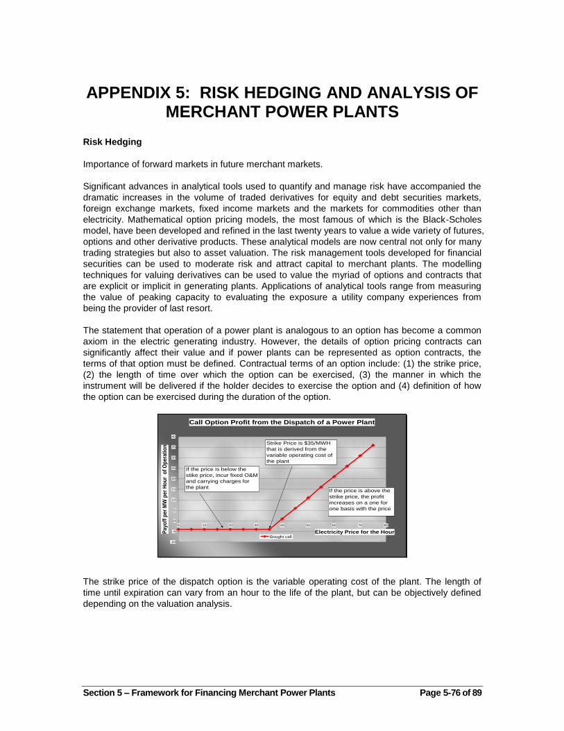
Section 5 – Framework for Financing Merchant Power Plants Page 5-76 of 89
APPENDIX 5: RISK HEDGING AND ANALYSIS OF MERCHANT POWER PLANTS
Risk Hedging
Importance of forward markets in future merchant markets.
Significant advances in analytical tools used to quantify and manage risk have accompanied the
dramatic increases in the volume of traded derivatives for equity and debt securities markets,
foreign exchange markets, fixed income markets and the markets for commodities other than
electricity. Mathematical option pricing models, the most famous of which is the Black-Scholes
model, have been developed and refined in the last twenty years to value a wide variety of futures,
options and other derivative products. These analytical models are now central not only for many
trading strategies but also to asset valuation. The risk management tools developed for financial
securities can be used to moderate risk and attract capital to merchant plants. The modelling
techniques for valuing derivatives can be used to value the myriad of options and contracts that
are explicit or implicit in generating plants. Applications of analytical tools range from measuring
the value of peaking capacity to evaluating the exposure a utility company experiences from
being the provider of last resort.
The statement that operation of a power plant is analogous to an option has become a common
axiom in the electric generating industry. However, the details of option pricing contracts can
significantly affect their value and if power plants can be represented as option contracts, the
terms of that option must be defined. Contractual terms of an option include: (1) the strike price,
(2) the length of time over which the option can be exercised, (3) the manner in which the
instrument will be delivered if the holder decides to exercise the option and (4) definition of how
the option can be exercised during the duration of the option.
Call Option Profit from the Dispatch of a Power Plant
-10
-5
0
5
10
15
20
25
30
35
40
0 10 20 30 40 50 60 70 80
Electricity Price for the HourPa
yo
ff p
er
MW
pe
r H
ou
r o
f O
pe
rati
on
Bought call
If the price is below the
stike price, incur fixed O&M
and carrying charges for
the plant
Strike Price is $35/MWH
that is derived from the
variable operating cost of
the plant
If the price is above the
strike price, the profit
increases on a one for
one basis with the price
The strike price of the dispatch option is the variable operating cost of the plant. The length of
time until expiration can vary from an hour to the life of the plant, but can be objectively defined
depending on the valuation analysis.