5.02 modelinglow-temperature geochemicalprocesses · modelinglow-temperature geochemicalprocesses...

5.02
Modeling Low-TemperatureGeochemical ProcessesD.K. Nordstrom
USGeological Survey, Boulder, CO, USA

5.02.1 INTRODUCTION
1 5.02.1.1 What Is a Model? 2
5.02.2 MODELING CONCEPTS AND DEFINITIONS
3 5.02.2.1 Modeling Concepts 3 5.02.2.2 Modeling Definitions 3 5.02.2.3 Inverse Modeling, Mass Balancing, and Mole Balancing 4
5.02.3 SOLVING THE CHEMICAL EQUILIBRIUM PROBLEM
6
5.02.4 HISTORICAL BACKGROUND TO GEOCHEMICAL MODELING
7
5.02.5 THE PROBLEM OF ACTIVITY COEFFICIENTS
8 5.02.5.1 Activity Coefficients 8 5.02.5.2 Saturation Indices 10
5.02.6 GEOCHEMICAL DATABASES
10 5.02.6.1 Thermodynamic Databases 11 5.02.6.2 Electrolyte Databases 11
5.02.7 GEOCHEMICAL CODES
11 5.02.7.1 USGS Codes 12 5.02.7.2 LLNL Codes 13 5.02.7.3 Miami Codes 13 5.02.7.4 The Geochemist’s Workbencht 13 5.02.7.5 REDEQL-MINTEQ Codes 13 5.02.7.6 Waterloo Codes 15 5.02.7.7 Harvie–Møller–Weare Code 15 5.02.7.8 Windemere Humic Aqueous Models 15 5.02.7.9 Additional Codes 16
5.02.8 WATER–ROCK INTERACTIONS
17 5.02.8.1 Aqueous Speciation 17 5.02.8.2 Modeling Sorption Reactions 18 5.02.8.3 Model Simulations of Mineral Reactions 18 5.02.8.4 Reactive-Transport Modeling in Streams 25 5.02.8.5 Geochemical Modeling of Catchments 25 5.02.8.6 Reliability of Geochemical Model Simulations 27
5.02.9 FINAL COMMENTS
29
ACKNOWLEDGMENTS
30
REFERENCES
31
A model takes on the quality of theory when it ab-stracts from raw data the facts that its inventor per-ceives to be fundamental and controlling, and putsthese into relation to each other in ways that werenot understood before—thereby generating predic-tions of surprising new facts.

H. F. Judson (1980), The Search forSolutions

1

5.02.1 INTRODUCTION

Geochemical modeling has become a popularand useful tool for a wide number of appli-cations from research on the fundamental proc-esses of water–rock interactions to regulatoryrequirements and decisions regarding permits

2 Modeling Low-Temperature Geochemical Processes

for industrial and hazardous wastes. In low-temperature environments, generally thought ofas those in the temperature range of 0–100 1Cand close to atmospheric pressure (1 atm¼1.01325bar¼ 101,325Pa), complex hydrobio-geochemical reactions participate in an arrayof interconnected processes that affect us, andthat, in turn, we affect. Understanding thesecomplex processes often requires tools thatare sufficiently sophisticated to portray multi-component, multiphase chemical reactionsyet transparent enough to reveal the maindriving forces. Geochemical models are suchtools. The major processes that are requiredto model include mineral dissolution and pre-cipitation; aqueous inorganic speciation andcomplexation; solute adsorption and desorpt-ion; ion exchange; oxidation–reduction, orredox transformations; gas uptake or pro-duction; organic matter speciation and com-plexation; evaporation; dilution; water mixing;reaction during fluid flow; reaction involvingbiotic interactions; and photoreaction. Theseprocesses occur in rain, snow, fog, dry atmos-phere, interactions with flora and fauna, vege-tative decay, soils, bedrock weathering, streams,rivers, lakes, groundwaters, estuaries, brines,and diagenetic environments. Geochemicalmodeling attempts to understand the redistri-bution of elements and compounds, throughanthropogenic and natural means, for a largerange of scale from nanometer to global.‘‘Aqueous geochemistry’’ and ‘‘environmentalgeochemistry’’ are often used interchange-ably with ‘‘low-temperature geochemistry’’to emphasize hydrologic or environmentalobjectives.

Recognition of the strategy or philosophybehind geochemical modeling is not often dis-cussed or explicitly described. Plummer (1984,1992) and Parkhurst and Plummer (1993) com-pare and contrast two approaches for modelinggroundwater chemistry: (1) ‘‘forward model-ing,’’ which predicts water compositions fromhypothesized reactions and user assumptionsand (2) ‘‘inverse modeling,’’ which uses specificwater, mineral, and isotopic compositions toconstrain hypothesized reactions. These ap-proaches simply reflect the amount of field in-formation available. With minimal informationon a site, a modeler is forced to rely on forwardmodeling. Optimal information would includedetailed mineralogy on drill cores or well cut-tings combined with detailed water analyses atvarying depths and sufficient spatial distribu-tion to follow geochemical reactions and mix-ing of waters along defined flow paths. Withoptimal information, a modeler will depend oninverse modeling.

This chapter outlines the main concepts andkey developments in the field of geochemicalmodeling for low-temperature environmentsand illustrates their use with examples. It pro-ceeds with a short discussion of what modelingis, continues with concepts and definitionscommonly used, and follows with a short his-tory of geochemical models, a discussion ofdatabases, the codes that embody models, andrecent examples of how these codes have beenused in water–rock interactions. An importantnew stage of development has been reached inthis field with questions of reliability and val-idity of models. Future work will be obligatedto document ranges of certainty and sources ofuncertainty, sensitivity of models and codes toparameter errors and assumptions, propagat-ion of errors, and delineation of the range ofapplicability.

5.02.1.1 What Is a Model?

A ‘‘model’’ has a relation to ‘‘reality,’’ butreality is experiential, and the moment we at-tempt to convey the experience we are seriouslyconstrained by three limitations: our own abil-ity to communicate, the capability of the com-munication medium to portray the experience,and the ability of the person receiving the com-munication to understand it. Communicationrequires the use of language and the use ofpercepts and concepts, and the process of per-ceiving, conceiving, and communicating is anabstracting process that removes us from theimmediate experience. Any attempt to trans-form an experience into language suffers fromthis abstraction process so that we lose the im-mediate experience to gain some understandingof it. The problem is to transform existentialknowledge to communicated or processed know-ledge and to eliminate unnecessary subjectivityfrom objective knowledge. To communicateknowledge, we must use a simplified and ab-stract symbolism (words, mathematics, pictures,diagrams, analogs, allegories, three-dimen-sional physical constructs, etc.) to describe amaterial object or phenomenon, that is, amodel. Models take on many forms but theyare all characterized by being a simplificationor idealization of reality. ‘‘ymodels includeonly properties and relationships that are neededto understand those aspects of the real systemthat we are interested iny’’ (Derry, 1999).Assumptions, both explicit and implicit, aremade in model construction, because either wedo not know all the necessary properties or we donot need to know them. Hopefully, models havecaught the essential properties of that which

Modeling Concepts and Definitions 3

they are attempting to portray so that they areuseful and lead to new insights and to betteranswers for existing questions and problems.

Science and scientific models begin as ideasand opinions that are formalized into alanguage, often, but not necessarily, mathe-matical language. Prior to the late nineteenthcentury, models (not usually called as such)were developed to explain and generalizeobservations of phenomena. Beginning in thelate nineteenth century, a new perspectivedeveloped in science that became known aslogical positivism. This perspective emphasizedthe predictive capability of science through hy-pothesis testing, or the hypothetico-deductivedescription of science and modeling. Usefuland rigorous science (and models) should havetestable consequences. The emphasis on testa-bility, or falsifiability, is considered a funda-mental attribute (Popper, 1934). Greenwood(1989) stated that the word model should bereserved ‘‘y for well-constrained logical prop-ositions, not necessarily mathematical, thathave necessary and testable consequences, andavoid the use of the word if we are merelyconstructing a scenario of possibilities.’’ Hence,a scientific model is a testable idea, hypothesis,theory, or combination of theories that pro-vides new insight or a new interpretation of anexisting problem. An additional quality oftenattributed to a model or theory is its ability toexplain a large number of observations whilemaintaining simplicity (Occam’s razor). Thesimplest model that explains most of theobservations is the one that will have the mostappeal and applicability.

Models are applied to a ‘‘system,’’ or a por-tion of the observable universe separated bywell-defined boundaries for the purpose ofinvestigation. A chemical model is a theoreti-cal construct that permits the calculation ofchemical properties and processes, such as thethermodynamic, kinetic, or quantum mechan-ical properties of a system. A geochemicalmodel is a chemical model developed forgeologic systems. Geochemical models oftenincorporate chemical models such as ion asso-ciation (IA) and aqueous speciation togetherwith mineralogical data and assumptions aboutmass transfer to study water–rock interactions.

A computer code is obviously not a model. Acomputer code that incorporates a geochemicalmodel is one of several possible tools for inter-preting water–rock interactions in low-temper-ature geochemistry. The computer codes incommon use and examples of their applicationwill be the main focus of this chapter. It isunfortunate that one commonly finds, in theliterature, reference to the MINTEQ model orthe PHREEQE model or the EQ3/6 model

when these are not models but computer codes.Some of the models used by these codes are thesame so that a different code name does notnecessarily mean a different model is being used.

5.02.2 MODELING CONCEPTS ANDDEFINITIONS

5.02.2.1 Modeling Concepts

Many different forms of models are utilized,usually dictated by the objectives of research.‘‘Conceptual models’’ are the most fundamen-tal. All of us have some kind of concept ofwater–rock interactions. For a groundwaterinteracting with aquifer minerals, one mightconceive that most minerals would be undersat-urated in the area of recharge but that someminerals (those that dissolve fastest) would be-come saturated at some point down gradient,having reached their equilibrium solubility (astate of ‘‘partial equilibrium’’). The conceptualmodel can be formalized into a set of mathe-matical equations using chemical principles, the‘‘mathematical model,’’ entered into a computerprogram, the ‘‘code,’’ and predictions made totest the assumptions (and the databases) againstthe results from real-field data. This exercisehelps to quantify and constrain the possible re-actions that might occur on the subsurface.Mathematical equations for complex interactingvariables are not always solved exactly and,therefore, systems of numerical approximations,or ‘‘numerical models,’’ have been developed.Alternatively, an experiment could be set up inthe laboratory with columns made of aquifermaterial with groundwater flowing through tosimulate the reactions, the ‘‘experimental mod-el’’ or ‘‘scale model.’’ Having obtained resultsfrom a mathematical or scale model, some un-expected results often occur which force us tochange our original conceptual model. This ex-ample demonstrates how science works; it is anongoing process of approximation that iteratesbetween idea, theory, observational testing oftheory, and back to modifications of theory ordevelopment of new theories.

5.02.2.2 Modeling Definitions

In low-temperature geochemistry and geo-chemical modeling, it is helpful to define severalwords and phrases in common use.

Aqueous speciation. The distribution of dis-solved components among free ions, ion pairs,and complexes. For example, dissolved ironin acid mine drainage (AMD) can be present

as Fe2þðaq:Þ (free ferrous iron), FeSO04ðaq:Þ (ion

pair), Fe3þðaq:Þ (free ferric iron), FeðOHÞ2þðaq:Þ, and


FeSOþ4ðaq:Þ species. These species are presentin a single-phase, aqueous solution. Aqueousspeciation is not uniquely defined but dependson the theoretical formulation of mass-actionequilibria and activity coefficients, that is, it ismodel dependent. Some aqueous speciation canbe determined analytically but operational def-initions and assumptions are still unavoidable.

Phase. Commonly defined as a uniform,homogeneous, physically distinct, and mechan-ically separable part of a system. Unfortunately,mineral phases are often not uniform, homo-geneous, or mechanically separable except intheory. Sophisticated microscopic and spec-troscopic techniques and operational definitionsare needed to define some mineral phases.Likewise, the aqueous solution phase can haveconcentration gradients based on density gra-dients that may be caused by temperature andcompositional differences.

Phase speciation. The distribution of compo-nents among two or more phases. For example,in a wet soil, iron can be present in at leastthree phases: as the X-ray amorphous oxyhy-droxide, ferrihydrite; as goethite; and as dis-solved aqueous iron.

Mass transfer. The transfer of mass betweentwo or more phases as in the precipitation anddissolution of minerals in a groundwater.

Reaction-path calculation. A sequence ofmass-transfer calculations that follows definedphase (or reaction) boundaries during incre-mental steps of reaction progress.

Mass transport. Solute movement by massflow of a fluid (could be liquid, gas, or mixtureof solid and liquid and/or gas).

Reactive transport. Mass transfer combinedwith mass transport; commonly refers to geo-chemical reactions during stream flow orgroundwater flow.

Forward geochemical modeling. Given an in-itial water of known composition and a rock ofknown mineralogy and composition, the rockand water are computationally reacted under agiven set of conditions (constant or variabletemperature, pressure, and water composition)to produce rock and water (or set of rocks andwaters). In forward modeling, the products areinferred from an assumed set of conditions(equilibrium or not, phases allowed to precip-itate or not, etc.) and thermodynamic and/orkinetic data are necessary.

Inverse geochemical modeling. Given a set oftwo or more actual water analyses along a flowpath that have already reacted with a rock ofknown mineralogy, the reactions are inferred.In inverse modeling the reactions are computedfrom the known field conditions (knownwater chemistry evolution and known miner-alogy) and assumed mineral reactivity. Inverse

modeling is based on mass or mole balancing,and thermodynamic and kinetic data are notnecessary although saturation indices provideuseful constraints. Relativistic kinetics (i.e., re-lative mineral reaction rates) are deduced aspart of the results.

5.02.2.3 Inverse Modeling, Mass Balancing,and Mole Balancing

A key concept to interpreting water–rock in-teractions is mass balancing between waterchemistry data, mineral/gas transformations,and biological uptake or release. The mass-balance concept is a means of keeping track ofreacting phases that transfer mass during fluidflow. It is an integral part of the continuityequation for steady-state and transient-stateflow conditions. Formalizing mass balancesfor solutes during fluid flow is simple if thesolutes are conservative but more complexwhen reactions take place. For applicationsto the environment, different types of massbalances have been used and these require someexplanation.

Three types of mass-balance approaches willbe discussed. In its simplest form, mass ba-lancing is utilizing the law of conservation ofmass that reflects that any partitioning of massthrough a system must sum to the total. Thefirst type of mass-balance approach, catchmentmass balances (or mass fluxes), uses ‘‘input–output’’ accounting methods to identify overallgains and losses of solutes during the flow ofwater from meteoric inputs to stream outflowat a specified point (Bormann and Likens,1967; Likens et al., 1977). Paces (1983, 1984)called this the integral mass-balance approach:

½Mass ratein �mass rateout�7mass rateinternal

¼ rate of accumulation=depletion ð1Þ

In difference form

Dmtrans

Dtþ Dmint

Dt¼ Dmtot

Dtð2Þ

where Dmtrans/Dt is the difference in rate ofmass (of some component) transported intoand out of the system via fluid flow, Dmint/Dtthe rate of mass produced or removed fromthe fluid by internal chemical reaction, andDmtot/Dt the total rate of change in mass for acomponent in the fluid. Steady-state conditionsare often assumed so that the accumulation/depletion rate becomes 0 and the differencebetween input and output for a component

Modeling Concepts and Definitions 5

becomes equal to the internal processes thatproduce or remove that component. Thesemass rates of change are usually obtained asintegral mass fluxes (computed as dischargetimes concentration).

For catchments in which input from precip-itation and dry deposition can be measured andthe output through a weir or similar confiningoutflow can be measured, the difference insolute flow averaged over an appropriate pe-riod of time provides an accounting of solutesgained or lost. Overviews and summaries ofessential concepts of catchment mass balanceshave been presented by Drever (1997a, b), Bas-sett (1997), and Bricker et al. (Chapter 5.04).The input–output mass balance treats thecatchment as a black box, but knowledge ofbiogeochemical processes, use of lab experi-ments, additional field data, and well-control-led small-scale field-plot studies can help toidentify the dominant processes causing thegain or loss of a particular solute. Load (ormass flux) calculations for a river or stream usethe same type of accounting procedure.

A second type of mass-balance approach isquantitative incorporation of mass balanceswithin a reactive-transport model and couldbe applied to groundwaters, surface waters,and surface water–groundwater interactions.Paces (1983, 1984) calls this the local mass-bal-ance approach. There are numerous examplesand explanations of this approach (e.g., Freezeand Cherry, 1979; Domenico and Schwartz,1990).

A third type of mass-balance approach is toleave the physical flow conditions implicit, as-sume steady-state flow along a flow line in anaquifer, and account for observed chemicalchanges that occur as the groundwater flowsfrom recharge to discharge (Plummer andBack, 1980). This approach was introducedformally by the classic paper of Garrels andMackenzie (1967), who calculated mass bal-ances derived from springwater data in the Si-erra Nevada Mountains of California. Themodeler begins with aqueous chemical dataalong a flow path in an aquifer (or catchment)of known mineralogy and accounts for changesin solute concentrations by specified reactionsources and sinks. The analytical solution isachieved by solving a set of simultaneous linearequations known as mole balancing:

Xj

j¼1bpai

p ¼ Dmi ¼ miðfinalÞ �miðinitialÞ ð3Þ

in which mi is the number of moles of element/component i per kilogram of water, ap

j the sto-ichiometric coefficient of element i in phase p,

bp the mass-transfer coefficient of the pthphase, and j the number of phases (Plummeret al., 1983). Because groundwaters are fre-quently mixtures of different water qualitytypes, mixing fractions can also be employedin the matrix array. Redox chemistry can beincluded through conservation of electrons andwater balance can be used to simulate evap-oration. Plummer (1984) has called this type ofmodeling the inverse method, because it pro-ceeds in a reverse manner to that of forwardmodeling, that is, it backs out the probable re-actions from known data on water chemistry,isotopes, and mineralogy. Parkhurst (1997)simply refers to it as mole balancing. Seman-tics aside, this model is developed for water–rock interactions from ‘‘a set of mixingfractions of initial aqueous solutions and moletransfers of minerals and gases that quanti-tatively account for the chemical compositionof the final solution’’ (Parkhurst, 1997).

Two papers point out the fundamental na-ture of mole balancing for interpreting ground-water chemistry. Plummer (1984) describesthe attempts to model the Madison Limestoneaquifer by both forward and inverse methods.Two valuable conclusions from this paper werethat information gained from mole balancingwas needed to provide relativistic reactionrates for forward modeling and that even withthese rates, the well water compositions couldnot be closely matched, whereas they can beexactly matched with inverse modeling. Fur-thermore, forward modeling required muchmore effort and contained more uncertainty.Similar conclusions were reached by Glynn andBrown (1996) in their detailed study ofthe acidic plume moving in the Pinal CreekBasin. They found that the best approach wasto pursue a series of mole-balance calculations,improving their modeling with each re-exami-nation of the phases and reactions considered.Then they took their refined mole-balance re-sults and made further improvements by for-ward modeling. Inverse modeling, however,was a key to their successful interpretation. Thecomplex nature of interpreting a dispersed con-taminant plume and the associated mineraldissolution front required the use of reactive-transport modeling. The reactive-transportmodeling, however, would have been muchmore uncertain without the inverse modeling atthe front end.

It has been pointed out that inverse model-ing assumes advective, steady-state flow andthat ‘‘reaction inversion’’ does not occur(Steefel and Van Cappellen, 1998). Althoughthese are important issues, they are oftennot serious limitations. These assumptionsare not a firm requirement for the system


being studied; it is only essential that the con-sequences of assuming them for non-steady-state flow (with or without dispersion) do nothave a significant effect on the results of thecalculation. For example, it can be argued thatover a long enough period of time or for alarge enough aquifer, steady-state conditionsnever truly apply. Indeed, steady state is anapproximation of the physical and chemicalstate of an aquifer system that works well formany, if not most, aquifers. As Zhu and And-erson (2002) pointed out, the most importantcriterion is that the same parcel of water hastraveled from point A to point B. They alsostate that chemical steady state is sufficient butnot necessary ‘‘because the underlying mathe-matical equations to be solvedy are theintegrated forms of mass conservation (Licht-ner, 1996).’’ At the Iron Mountain mines (Al-pers et al., 1992), high concentrations of sulfate(tens of grams per liter) and metals (grams perliter) discharge from two major portals. Thegroundwater has advective and nonadvective(dispersive and convective) properties, and thevariable effluent flows would indicate transientstate. The chemistry, however, is still domi-nated by oxidation of sulfide minerals and aciddissolution of aluminosilicate minerals, and amass-balance calculation will still reflect thesegeochemical processes. A mass balance goingfrom rainwater to portal effluent will delineatethe key minerals that dissolve and precipitatealong the flow path. Steefel and Van Cappellen(1998) correctly state that inverse modelingcannot be applied to contaminant plumes orreaction fronts unless the spatial delineation ofthe reaction front is clearly defined. ‘‘Reactioninversion,’’ such as the dissolution of a partic-ular mineral changing to precipitation betweentwo points along a flow path such that nooverall reaction appears to have taken place, isan interesting problem. Without additional in-formation it would not be possible to dis-tinguish between no reaction and reactioninversion. In such instances, it makes no dif-ference to the modeling or the conclusions,because the net result is the same. It is as if theelement of concern was conserved in the solidphase during that increment of fluid flow, asafe assumption for silica in quartz but notfor silica from weathering feldspars. It mightonly matter if these small-scale processesaffect other processes such as the unidirec-tional release or attenuation of trace elements(released upon mineral dissolution but notcoprecipitated or adsorbed upon mineral pre-cipitation or vice versa) or similar irreversibleprocesses involving nutrients. Further discus-sion of inverse modeling is found in Sections5.02.7.1 and 5.02.8.3).

5.02.3 SOLVING THE CHEMICALEQUILIBRIUM PROBLEM

Although both kinetic and equilibrium ex-pressions can be used in geochemical modelingcomputations, the ‘‘equilibrium problem’’ isthe foundation of most calculations of thistype. Simply stated, the chemical equilibriumproblem is the determination of the most stablestate of a system for a given set of pressure P,temperature T, and compositional constraintsXi. These variables, P, T, and Xi, need not befixed, but they must be defined for the givensystem. The chemical state of a system is givenby the total Gibbs free energy, G, and itsdifferential change with the progress variable,x, denotes the state of the system in mathe-matical terms. For a system at equilibrium

@G

@x

� �P;T

¼ 0 ð4Þ

and any perturbation from equilibrium willcause this differential to be other than 0. Theprogress variable is a singular quantity thatexpresses the extent to which a reaction hastaken place. It is equal to the change in thenumber of moles, ni, of a reactant (or product)normalized to the stoichiometric coefficient, ni,for that component, element, or species. In dif-ferential form,

@x ¼ @ni

vi

ð5Þ

Solving the equilibrium problem means fin-ding the minimum in the free-energy curve forthe defined system. Two general approacheshave been used: the equilibrium constant ap-proach and the free-energy minimization ap-proach. As the names suggest they primarilyuse equilibrium constants to solve the problemor they use free energies. Of course, the ap-proaches are considered the same because theyare related by DrG1¼RT ln K, where R is theuniversal gas constant, T the absolute temper-ature in kelvin, and K the equilibrium constant,but the logarithmic conversion leads to differ-ent numerical techniques. Both approacheshave to employ mass-balance and mass-actionequations. Upon substitution of mass-actioninto mass-balance expressions (or vice versa), aset of nonlinear equations is derived that arereadily solved by a numerical method codedfor a computer. The mathematical formulationof the chemical equilibrium problem is ex-plained in Zeleznik and Gordon (1968), VanZeggeren and Storey (1970), Wolery (1979), andSmith and Missen (1982). Harvie and Weare(1980) and Harvie et al. (1987) have improved

Historical Background to Geochemical Modeling 7

the free-energy minimization algorithm forsolving the general chemical equilibrium prob-lem and applied it to finding parameters for thePitzer method. Rubin (1983, 1990) providesmore formalism for dealing with reactive trans-port and nonequilibrium conditions. Furtherdiscussion of the numerical techniques can befound in the books by Smith and Missen(1982), Nordstrom and Munoz (1994), andmany other textbooks and papers. A simpleproblem involving speciation of an aqueoussolution at equilibrium with gypsum is solvedby both the Newton–Raphson method and the‘‘continued fraction’’ method in Nordstromand Munoz (1994).

5.02.4 HISTORICAL BACKGROUND TOGEOCHEMICAL MODELING

The founders of geochemistry, F. W. Clarke,G. M. Goldschmidt, V. I. Vernadsky, and A. E.Fersman, clearly made major contributions toour ‘‘models’’ of geochemical processes. Today,however, we think of geochemical models interms of high-speed quantitative computationsof water–rock interactions made possiblewith fast processors and disks with large mem-ories. This direction of research began with theprinciples of physical chemistry adapted forsolving aqueous low-temperature geochemicalproblems by Hem (1959), Garrels (1960), Sillen(1961), Garrels and Christ (1965), and Kraus-kopf (1967). The scholarly structures that theseauthors built would not have been possiblewithout the foundations laid by those whocame before and developed the science of phys-ical chemistry: Wilhelm Ostwald, JacobiusHenricus van’t Hoff, and Svante Arrhenius(Servos, 1990). These chemists, along withnumerous others they influenced, establishedthe principles upon which aqueous low-tem-perature geochemistry and geochemical model-ing is based. Van’t Hoff himself was an earlydeveloper of geochemical models in his effortsto apply physical chemistry to the interpreta-tion of the equilibrium factors determiningthe stability of gypsum and anhydrite (van’tHoff et al., 1903) and the equilibrium interpre-tation of the Permian Zechstein evaporite de-posits (van’t Hoff 1905, 1909, 1912; Eugster,1971).

Probably the earliest paper to apply aspeciation calculation to natural water wasGoldberg’s (1954) estimate of the differentforms of dissolved copper in seawater basedon Niels Bjerrum’s theory of ion-pair forma-tion and Jannik Bjerrum’s data (see Bjerrum,1950). He found that 65% was in the freeion (Cu2þ ) form and another 33% was present

as either a cation or neutral species form(copper-chloride complexes). This calculation,however, did not take into account simultane-ous competitive complexing from all the otherions in seawater. Speciation was central toKrauskopf’s (1951) study on gold solubility,his discussion of trace-metal enrichment in sedi-mentary deposits (Krauskopf, 1955), and hisexamination of the factors controlling trace-metal concentrations in seawater (Krauskopf,1956). In the US Geological Survey (USGS),Hem and Cropper (1959) and Hem (1961) wereestimating distribution of ionic species andactivities of ions at chemical equilibrium in nat-ural waters. Sillen’s (1961) first paper on sea-water considered hydrolysis and complexformation. At this time he and his colleagueswere pioneering the application of computers tosolve complex aqueous solution equilibria(Sillen, 1962; Ingri and Sillen, 1962; Ingriet al., 1967; Dyrssen et al., 1968). A classic pa-per that applied aqueous speciation to naturalwater was that of Garrels and Thompson (1962)in their ‘‘Chemical Model of Seawater,’’ whichcontained unique features such as the mean-saltmethod for estimating activity coefficients.

The adaptation of water–rock geochemicalmodeling to computers was pioneered byHelgeson and his colleagues, who focusedon ore deposits and high-temperature, high-pressure reactions (Helgeson, 1964, 1967, 1969)but also considered low-temperature processes(Helgeson et al., 1969, 1970). Helgeson’s (1971)research continued with the application ofcomputers to the calculation of geochemicalkinetics. Theoretical approaches were devel-oped for geochemical kinetics (Aagard andHelgeson, 1982; Helgeson and Murphy, 1983)and computations compared with measuredreaction rates (Helgeson et al., 1984; Murphyand Helgeson, 1987) and coupled with diffu-sion (Murphy et al., 1989). These approachesprovide an insight to the mechanisms of con-trolled laboratory studies on mineral dissolu-tion rates, but difficulties are encountered whenapplications are made to the complex condi-tions of the natural environment. Experimentaland theoretical approaches to mineral dissolu-tion fail to predict the actual dissolution ratesin catchments, because experiments do not re-produce the composition and structure of nat-ural mineral surfaces, they do not account foradsorbed inhibitors, they do not consider theeffect of variable climate and hydrologic flowrates, and they do not account for biologicalactivity. These factors may have taken any-where from decades to millenia to develop andthey can change over short periods of time.Computer codes that incorporate reactionkinetics into groundwater or catchment codes


usually do so with some type of general-ized first-order rate law.

Beginning in the 1960s and expanding con-siderably during the 1970s, a series of computercodes were developed that could perform awide variety of aqueous geochemical calcula-tions (Bassett and Melchior, 1990; Mangoldand Tsang, 1991) and these evolved consider-ably during the 1980s and 1990s to includesimulation of more processes, coupling ofprocesses (especially reaction with transport),and the availability of more options (Alpersand Nordstrom, 1999). The advances ingeochemical modeling are apparent in theevolution of Barnes’ Geochemistry of Hydro-thermal Ore Deposits from first edition (Barnes,1967) to third edition (Barnes, 1997), in theAmerican Chemical Society (ACS) booksChemical Modeling in Aqueous Systems thathave shown significant advances from thefirst (Jenne, 1979) to the second (Melchiorand Bassett, 1990), and in the plethora of pa-pers on this subject since the 1980s. Neverthe-less, advanced sophistication for geochemicalcodes does not imply a parallel advance in ourunderstanding of geochemical processes. Thesophistication of software has outdistancedour capacity to evaluate the software over arange of conditions and it has outdistanced ourability to obtain the field data to constrain andtest the software.

5.02.5 THE PROBLEM OF ACTIVITYCOEFFICIENTS

5.02.5.1 Activity Coefficients

Aqueous electrolytes and the equilibriumconstants that define various reactions in low-temperature geochemistry are inexorablylinked with the problem of activity coefficients,or the problem of nonideality for aqueous elec-trolyte solutions. Thermodynamic equilibriumconstants, defined by an extrapolation to infi-nite dilution for the standard state condition(not the only standard state), require the use ofactivity coefficients. Unfortunately, there isneither a simple nor universal nonidealitymethod that works for all electrolytes underall conditions. This section provides a briefoverview of a major subject still undergoingresearch and development but for which severalsatisfactory approaches are available.

If the activity of a solute or ion were ideal, itcould be taken as equivalent to the molal con-centration, mi, of the i ion or solute. However,interactions with other ions and with thesolvent water are strong enough to cause non-ideal behavior, and the characteristic property

relating concentration to chemical potential isthe activity coefficient, gi:

ai ¼ gimi ð6Þ

With the accumulation of activity coefficientmeasurements and the search for a theoreticalexpression ensued, it was discovered that indilute solutions the logarithm of the activitycoefficient was an approximate function of thesquare root of the molality:

ln gi ¼ �aim1=2i ð7Þ

where ai was simply a constant. Brønsted(1922) introduced a linear term to Equation(7) in which the coefficient, b, is a ‘‘specific-ioninteraction parameter,’’

ln gi ¼ �aim1=2i � bmi ð8Þ

Later modifications of this general approachbecame known as the specific-ion interactiontheory (SIT) because of the explicit dependenceon the solute or ions being considered.

An important concept that aided in thedevelopment of electrolyte theory was the ionicstrength, I, introduced by Lewis and Randall(1921):

I ¼ 1

2

Xmiz

2i ð9Þ

where zi is the ionic charge. Thereafter, theionic strength was used as a parameter inactivity coefficient equations. Debye and Huck-el (1923) derived an equation from electrostatictheory which, in the limit of infinite dilution(hence, the Debye–Huckel limiting law),becomes

log gi ¼ �Az2i I1=2 ð10Þ

where A is a Debye–Huckel solvent parameter(dependent on the properties of the solvent).

The extended Debye–Huckel equation is

log gi ¼ �Az2i I1=2

1þ BaiI1=2ð11Þ

where B is another Debye–Huckel solvent pa-rameter and ai is an ion-size diameter derivedby empirical fit but approximates the hydratedion diameter.

The use of the extended Debye–Huckel equa-tion with the appropriate equilibrium constants

The Problem of Activity Coefficients 9

for mass-action expressions to solve a complexchemical equilibrium problem is known as theIA method.

Several modifications of these equationswere tried over the next several decades. Con-tributions by Guggenheim (1935) and Scat-chard (1936) and the KTH or Swedish group(Grenthe et al., 1992, 1997) became theBrønsted–Guggenheim–Scatchard or SITmethod:


1þ 1:5I1=2þX

k

eði; k; IÞmk ð12Þ

Here the linear term is a function of molalitysummed for all the other ions in solutions,k, and e(i, k,I) tends to be constant at highermolalities but solute or ion specific. Thelast term in Equation (12) represents the deviat-ion of the experimentally measured activitycoefficient from the prediction of the Debye–Huckel equation. Other groups, such asTruesdell and Jones (1974), kept the ionicstrength dependence throughout the equation,and the coefficient, b, became the differencefactor but still a constant for a given soluteor ion:


1þ BaiI1=2þ biI ð13Þ

The IA method using Equation (13) for ma-jor ions in natural water compares well withother more precise methods (see below) up toan ionic strength of seawater (0.7) but notmuch higher.

The next better approximation is to allowthe linear coefficient to be a function of the ionicstrength (Pitzer and Brewer, 1961) and it wasutilized by Helgeson and Kirkham (1974a, b,1976), Helgeson et al. (1981), and Tanger andHelgeson (1988) in the development of theHelgeson–Kirkham–Flowers (HKF) equations,which include consideration of the Born func-tion and ion hydration.

Pitzer (1973) reexamined the statisticalmechanics of aqueous electrolytes in waterand derived a different but semiempiricalmethod for activity coefficients, commonlytermed the Pitzer specific-ion interactionmodel. He fitted a slightly different functionfor behavior at low concentrations and used avirial coefficient formulation for high concen-trations. The results have proved extremelyfruitful for modeling activity coefficients overa very large range of molality. The general

equation is

ln g7 ¼ �A

3jzþz�jf ðIÞ þ

2uþu�u

BðIÞm

þ 2ðuþu�Þ3=2

uCm2 ð14Þ

where

f ðIÞ ¼ I1=2

1þ 1:2I1=2þ 1:67 lnð1þ 1:2I1=2Þ

and

BðIÞ ¼ 2b1

þ 2b0

a2I1� 1þ aI1=2 � 1

2a2I

� �e�aI1=2

� �

in which b1 and b0 are specific-ion parameters, ais a constant for a similarly charged classof electrolytes, and C a specific-ion parameterindependent of ionic strength. The B and Cparameters are second and third virial coeffi-cients. The parameter v¼ vþ þ v–, is the sum ofthe stoichiometric coefficients for the cation,vþ , and the anion, v–, of the solute. The Pitzerparameters have been fitted for a wide range ofsolutes and have been used for mixed electrolytesolutions to model the mineral solubilitybehavior in brines (Harvie and Weare, 1980;Harvie et al., 1980). Grenthe et al. (1997) com-pared the SIT method and the Pitzer method indetail and came to the following conclusions:(1) the more extensively parametrized Pitzermodel allows the most precise modeling ofactivity coefficients and equilibrium constantsprovided that all the interaction coefficients areknown; (2) when Pitzer parameters are missing(not available from experimental data), theymust be estimated and the precision and accu-racy of the activity coefficients can be signi-ficantly compromised; (3) the parameters in theSIT model can be related to those in the Pitzermodel and provide another means of estimatingPitzer parameters; (4) the SIT model is in goodagreement with the Pitzer model for the rangem¼ 0.1–4mol kg–1; and (5) the Pitzer model isthe preferred formalism for solutions or brinesof high ionic strength. An extensive discussionof the development of the Pitzer model andseveral hybrid approaches can be found in Pit-zer (1991a) and Millero (2001). It appears thathybrid approaches provide the best promise inthe future, because they combine the extensivedata available on equilibrium constants with abetter formulation of activity coefficients.

The difference between the extended Debye–Huckel equation and the Pitzer equations


concerns with how much of the nonideality ofelectrostatic interactions is incorporated intomass-action expressions and how much into theactivity coefficient expression. It is importantto remember that the expression for activitycoefficients is inexorably bound up with equi-librium constants and they must be consistentwith each other in a chemical model. Ion-pairinteractions can be quantified in two ways, ex-plicitly through stability constants (IA method)or implicitly through empirical fits with activitycoefficient parameters (Pitzer method). Bothapproaches can be successful with enougheffort to achieve consistency. At present, thePitzer method works much better for brines,and the IA method works better for dilute wa-ters because of the greater number of compo-nents and species for which basic data exist.When the effort is made to compare both ap-proaches for the same set of high-quality data,they appear to be comparable (Felmy et al.,1990). The primary challenge for the future willbe to insure that consistency is maintained be-tween the thermodynamic data, the expressionsfor nonideality, and the mass-action expres-sions in geochemical modeling codes, and toincorporate trace elements and redox specieswithin the same formulation.

5.02.5.2 Saturation Indices

After speciation and activities have been cal-culated for all the free ions, ion pairs, triplets,etc., a mineral saturation index can be com-puted. The saturation index (SI) is defined asthe logarithm of the ratio of the ion-activityproduct (IAP) to the solubility product con-stant, Ksp,

SI ¼ logIAP

Ksp

� �ð15Þ

If the solution is at equilibrium, theIAP¼Ksp and the SI¼ 0. If the SI40, thenthe solution is supersaturated and the mineralwould tend to precipitate; if the SIo0, the so-lution is undersaturated and the mineral wouldtend to dissolve, if present. Because the SI isaffected by the stoichiometry of the mineralformula, it is best to normalize the SI to thetotal mineral stoichiometry as pointed out byZhang and Nancollas (1990):

SI ¼ logIAP

Ksp

� �1=uð16Þ

where v¼ vþ þ v–, is the sum of the stoic-hiometries of the positive and negative compo-nents in the mineral formula.

These computations describe the ‘‘tendency’’of a water sample to be saturated, but they donot necessarily demonstrate whether mineraldissolution or precipitation actually happens.For dissolution to occur, the mineral must bepresent and it must dissolve at a rate that is fastenough relative to the flow rate of the water toaffect the water chemistry (Berner, 1978). Like-wise for a mineral to precipitate, it must precip-itate at a rate fast enough to affect the waterchemistry. The kinetics of precipitation and dis-solution reactions must be applied to get a re-alistic interpretation of water–rock interactions.

5.02.6 GEOCHEMICAL DATABASES

Input for aqueous geochemical codes con-sists of field data (geology, petrology, miner-alogy, and water analyses), thermodynamicand aqueous electrolyte data, and possiblykinetic and sorption data. Thermodynamicdata are fundamental to most geochemicalcomputations and several major compilationsare available. Although the guidelines and nec-essary relations for thermodynamic consistencyare well established (Rossini et al., 1952;Helgeson, 1968, 1969; Haas and Fisher, 1976;Nordstrom et al., 1990; Nordstrom andMunoz, 1994), it has been difficult to employthem in the development of databases. Twogeneral approaches have been recognized, serialnetworks and simultaneous regression. Withserial networks, an evaluator begins with asingle starting point, such as the standard stateproperties for an element (or all elements)and gradually builds in the properties ofcompounds through the appropriate reactioncombinations. Serial networks, such as thatdeveloped by the National Bureau of Standards(formerly NBS, now NIST, National Instituteof Standards and Technology) database (Wag-man et al., 1982), achieve continuity for a largedata set but lose thermodynamic constraints,whereas simultaneous regression, which pre-serves thermodynamic relationships, can onlybe done on a limited subset of data, andthe weighting of the regression fit dependson the judgment of the evaluator (Archerand Nordstrom, 2003). Computer codeshave been developed for the purpose of corre-lating and evaluating a diversity of thermody-namic data (Haas, 1974; Ball et al., 1988), butthey have not been widely used. Seriousdiscrepancies in thermodynamic properties doappear among these compilations and someof these discrepancies have been incorporatedinto the databases of geochemical codes. Manyusers of these codes are not familiar withthese databases and the possible uncertainties

Geochemical Codes 11

propagated through the computations fromthermodynamic errors. Such error propagationmay or may not be important, depending onthe specific objectives of the geochemical prob-lem being addressed.

5.02.6.1 Thermodynamic Databases

Since the early compilations of thermo-dynamic data (e.g., Lewis and Randall, 1923),numerous measurements were made during thetwentieth century leading to the well-knowncompilations of Latimer (1952) and Rossiniet al. (1952). Measurements and compilationscontinued to expand through the later partof the twentieth century, and comprehensiveinventories such as Sillen and Martell (1964),Martell and Smith (1974–76), Wagman et al.(1982), Chase (1998), Robie and Hemingway(1995), and Gurvich et al. (1993) summarizedand organized a considerable amount of data.Unfortunately, the methods used to evaluatethe data are not always transparent and occa-sionally the source references are not known.Notable exceptions were the publication of theCODATA tables (Garvin et al., 1987; Coxet al., 1989), the Organization Economic Co-operation and Development/Nuclear EnergyAgency Thermochemical Data Base (OECD/NEA TDB) publications (Grenthe et al., 1992;Silva et al., 1995; Rard et al., 1999; Lemireet al., 2001; Guillaumont et al., 2003), and theInternational Union of Pure and AppliedChemistry (IUPAC) compilations (e.g., Lam-bert and Clever, 1992; Scharlin, 1996). TheOECD/NEA TDB, although focusing on ra-dionuclides of most concern to safe disposal ofhigh-level radioactive wastes and militarywastes, contains a considerable amount of aux-iliary data on other common aqueous and solidspecies that had to be evaluated along with theactinides. For aqueous geochemical modeling,the equilibrium-constant tables of Nordstromet al. (1990) have proved to be useful andare found in USGS and US EnvironmentalProtection Agency (USEPA) codes describedbelow and in popular water-chemistry/aqueous-geochemistry textbooks (Appelo and Postma,1993; Stumm and Morgan, 1996; Langmuir,1997; Drever, 1997a). These tables have beenrecompiled, expanded, and tabulated in termsof thermodynamic properties (G, H, S, CP, andlog K for reaction and individual species (Nor-dstrom and Munoz, 1994)). The tabulationof Nordstrom and Munoz (1994) was organi-zed in such a way that individual species can becompared with reactions involving those spe-cies that were measured independently. Conse-quently, it is easy to check thermodynamic

relations to see if the properties for individualspecies are consistent with tabulated reactionequilibria. Only values that agreed within aclose range of the stated uncertainties wereincluded in the tables.

These tabulations represent a portion ofthe data needed for geochemical model com-putations and there have been some obviousinconsistencies. By the mid-1990s, critical eval-uations of thermodynamic data were taperingoff and many errors and inconsistencies hadnot been resolved. Even as of 1994, serious in-consistencies still existed between calorimetric-ally derived and solubility-derived propertiesfor such common minerals as celestine and ba-rite, and a less common but important phasesuch as radium sulfate (Nordstrom and Mu-noz, 1994). This set of discrepancies has beenresolved for celestine (SrSO4) and barite(BaSO4) by new measurements using high-tem-perature oxide-melt and differential-scanningcalorimetry (Majzlan et al., 2002). Listing ofsources of thermodynamic data compilationscan be found in Nordstrom and Munoz (1994)and in Grenthe and Puigdomenech (1997).

5.02.6.2 Electrolyte Databases

The classic books by Harned and Owen(1958) and Robinson and Stokes (1959) putelectrolyte theory on a firm basis and providedimportant tabulations of electrolyte data forcalculations of activity coefficients and relatedproperties. Advances in electrolyte theory,especially the use of the Pitzer method (Pitzer,1973, 1979), led to alternate methods of calcu-lating activities and speciation. The books ed-ited first by Pytkowicz (1979) and later byPitzer (1991b) provided a general overview ofthe different approaches and hybrid ap-proaches to these computations. A more re-cent reference providing a thorough overviewof the subject with tables of molal properties,activity coefficients and parameters, and disso-ciation/association constants is Millero (2001).These references explain the general use of theIA method with extended forms of Debye–Huckel equations, the Pitzer specific-ion inter-action method, and hybrid approaches thattake advantage of the best aspects of bothapproaches.

5.02.7 GEOCHEMICAL CODES

This listing and description of geochemicalcodes is not meant to be either exhaustiveor complete. It is meant to be a brief overviewof several codes in current and commonuse. Reviews by Yeh and Tripathi (1989a),


Mangold and Tsang (1991), Parkhurst andPlummer (1993), and Alpers and Nordstrom(1999) provide information on more codes,their evolution, and references to earlier re-views on codes and geochemical modeling.Loeppert et al. (1995) also contain useful in-formation on geochemical codes and modeling,especially for soil interactions. It is importantto remember that most codes in active use oftenundergo enhancements, database updates, andother improvements. The descriptions given inthis section may not apply to some of thesesame codes 5 years from now.

5.02.7.1 USGS Codes

The USGS has developed several codes thatare useful for the interpretation of water–chem-istry data and for simulating water–rock inter-actions. Two similar aqueous-speciation codeswere developed in parallel, WATEQ (Truesdelland Jones, 1974) and SOLMNEQ (Kharakaand Barnes, 1973). The primary aim of theseprograms was to aid in the interpretation ofwater-quality data. SOLMNEQ, however, hada different subroutine for calculating tempera-ture and pressure dependence and could calcu-late reaction equilibria above 100 1C. WATEQwas intended for temperatures of 0–100 1C.Both of these programs have been updated.WATEQ4F v.2 (Ball and Nordstrom, 1991,with database updates to 2002) uses the IAmethod with an expanded form of the extendedDebye–Huckel equation for major ions (theTruesdell–Jones formulation or hybrid-activitycoefficient; Truesdell and Jones (1974) andNordstrom and Munoz (1994), includes inde-pendent redox speciation computations thatassume redox disequilibrium, and has databaseupdates for uranium (Grenthe et al., 1992),chromium (Ball and Nordstrom, 1998), andarsenic redox species (Archer and Nordstrom,2003; Nordstrom and Archer, 2003). SOL-MINEQ. 88 (Kharaka et al., 1988; Perkinset al., 1990) covers the temperature range of0–350 1C and 1–1,000 bar pressure, includesboth the IA method and the Pitzer method,and has mass-transfer options such as boiling,fluid mixing, gas partitioning, mineral precip-itation, mineral dissolution, ion exchange, andsorption. It has been found to be particularlyapplicable to deep sedimentary basins, espe-cially those containing oil and gas deposits. Thelatest version, SOLMINEQ.GW is explained inan introductory text on groundwater geochem-istry (Hitchon et al., 1996).

Parkhurst et al. (1980) developed thePHREEQE code to compute, in addition toaqueous speciation, mass transfer, and reaction

paths. A separate but similar code, PHRQ-PITZ, uses the Pitzer method for brine calcu-lations (Plummer et al., 1988; Plummer andParkhurst, 1990). The PHREEQE code hasbeen regularly enhanced and the recent version,PHREEQC v. 2, includes ion exchange, evap-oration, fluid mixing, sorption, solid-solutionequilibria, kinetics, one-dimensional transport(advection, dispersion, and diffusion into stag-nant zones or dual porosity), and inverse mod-eling (Parkhurst and Appelo, 1999). Aninterface (PHREEQCI) was developed for in-teractive modification of the input files byCharlton et al. (1997). The latest developmentis PHAST, which includes three-dimensionaltransport (Parkhurst et al., 2004). The programPHAST uses the solute-transport simulatorHST3D (Kipp, 1987, 1998) and iterates atevery time step with PHREEQC. Thorstensonand Parkhurst (2002) have developed the the-ory needed to calculate individual isotope equi-librium constants for use in geochemicalmodels and utilized them in PHREEQC to cal-culate carbon-isotope compositions in unsatu-rated zone with seasonally varying CO2

production (Parkhurst et al., 2001).Geochemical modeling of reactants in flow-

ing mountainous stream systems can be donewith the USGS codes OTIS (Runkel, 1998) andOTEQ (Runkel et al., 1996, 1999) that modelsolute transport and reactive transport, re-spectively. OTIS, or one-dimensional transportwith inflow and storage, is based on the earlierwork of Bencala (1983) and Bencala and Wal-ters (1983). The OTEQ code combines theOTIS code with MINTEQA2 for chemical re-action at each incremental step of transport.These codes are calibrated with constant-flowtracer injection studies and testable assump-tions regarding the solubility product constantof the precipitating phases (Kimball et al.,2003). They have been tested in numeroussettings, primarily with the objective of quan-tifying and predicting the sources, transport,and fate of acid drainage from mined environ-ments in the western United States.

Codes for inverse modeling began withthe program BALANCE (Parkhurst et al.,1982) from which the interactive code NET-PATH (Plummer et al., 1991) evolved. NET-PATH, in addition to mass balances, doesdatabase management for a suite of wells andcan compute speciation and saturation indiceswith WATEQ. NETPATH has now been in-corporated into PHREEQC along with uncer-tainty propagation (Parkhurst, 1997). Bowserand Jones (1990, 2002) have incorporatedthe mass-balance approach into a spreadsheetformat that allows graphical output and aquick reconnaissance of ranges of mineral


compositions that are permissible models forsilicate solid-solution series (see Chapter 5.04).

USGS codes and manuals can be download-ed free of charge at Water Resources Applica-tions Software (2006). The more currentversion and additional bibliographic and infor-mation files for PHREEQC are available atReaction-Transport Modeling in Ground-Water Systems (2006). Updates on WATEQ4Fand revised thermodynamic data can be foundat Chemical Modeling of Acid Waters (2006).The OTIS code can be accessed at OTIS (2006).

5.02.7.2 LLNL Codes

A set of computer codes known as EQ3/6was originally developed by Wolery (1979) tomodel rock–water interactions in hydrothermalsystems for the temperature range 0–300 1C.Software development was later sponsored bythe US Department of Energy at LawrenceLivermore National Laboratories (LLNL) tomodel geochemical processes anticipated inhigh-level nuclear waste repositories. This geo-chemical code has become one of the most so-phisticated and most applicable for a widerange of conditions and processes. In additionto speciation and mass-transfer computations,it allows for equilibrium and nonequilibriumreactions, solid-solution reactions, kinetics, IA,and Pitzer methods, and both inorganic andorganic species. The program has been used forseveral municipal and industrial waste situa-tions and has been used to assess natural andengineered remediation processes. It has fivesupporting thermodynamic data files and thethermodynamic data are evaluated and up-dated with the SUPCRT92 software (Johnsonet al., 1992), based on Helgeson’s formulationfor activity coefficients and aqueous thermo-dynamic properties over a wide range of tem-perature and pressure (Helgeson and Kirkham,1974a, b, 1976; Helgeson et al., 1981) and solid-phase thermodynamic properties (Helgesonet al., 1978). Thermodynamic data are updatedwith the availability of published research (e.g.,Shock and Helgeson, 1988, 1990; Shock et al.,1989). Several manuals for operationand general information are available at IPAC(2006).

5.02.7.3 Miami Codes

It would be difficult to find more compre-hensive or more detailed studies on the physicalchemistry of seawater than those done at theUniversity of Miami (Millero, 2001). Severalcodes were developed for calculation of activitycoefficients and speciation of both major ions

and trace elements in seawater. The activitycoefficient models have been influencedstrongly by the Pitzer method but are best de-scribed as hybrid because of the need to useion-pair formation constants (Millero andSchreiber, 1982). The current model uses QBA-SIC; computes activity coefficients for 12 majorcations and anions, 7 neutral solutes, and morethan 36minor or trace ions. At 25 1C, the ionicstrength range is 0–6m. For major compo-nents, the temperature range has been extendedto 0–50 1C, and in many cases the temperaturedependence is reasonably estimated to 75 1C.Details of the model and the parameters andtheir sources can be found in Millero and Roy(1997) and Millero and Pierrot (1998). Com-parison of some individual ion activity coeffi-cients and some speciation for seawatercomputed with the Miami model is shown inSection 5.02.8.6 on model reliability.

5.02.7.4 The Geochemist’s Workbencht

A set of five programs known as The Geo-chemist’s Workbencht or GWB was developedby Bethke (1994) with a wide range of capabil-ities similar to EQ3/6 and PHREEQC v.2.GWB performs speciation, mass transfer, reac-tion-path calculations, isotopic calculations,temperature dependence for 0–300 1C, inde-pendent redox calculations, and sorption cal-culations. Several electrolyte databases areavailable including IA with Debye–Huckelactivity coefficients, the Pitzer formulation,the Harvie–Møller–Weare formulation, anda PHRQPITZ-compatible formulation. Theprogram X2t allows the coupling of two-di-mensional transport with geochemical reaction.Basin3 is a basin-modeling program that can belinked to GWB. Another advantageous featureis the plotting capability that can produce pe–pH or activity–activity or fugacity–fugacitydiagrams from GWB output. Bethke (1996)has published a textbook on GeochemicalReaction Modeling that guides the readerthrough a variety of geochemical computationsusing GWB and provides the basis for acourse in modeling. The GWB is a registeredcode and can be obtained from RockWare,Inc (RockWare, Inc. Earth Science & GISSoftware (2006)).

5.02.7.5 REDEQL-MINTEQ Codes

One of the first speciation programs thatincluded mass-transfer reactions at equilibriumwas REDEQL (Morel and Morgan, 1972). The


primary aim of this set of codes was to computethe equilibrium chemistry of dilute aqueoussolutions in the laboratory and was among thefirst to include sorption. It also has been widelyused to interpret water quality in environmen-tal systems. This FORTRAN code has evolvedthrough several versions, parallel with advan-ces in computer hardware and software. Incor-poration of the WATEQ3 database (Ball et al.,1981) with the MINEQL program (Westallet al., 1976) produced MINTEQ (Felmy et al.,1984) which became the USEPA-supportedcode, MINTEQA2 (Allison et al., 1991). Themore recent upgrade is MINTEQA2/PROD-EFA2 v. 4 (USEPA, 1998, 1999 (revised)), andcontains code revisions, updates in thermody-namic data, and modifications to minimizenonconvergence problems, to improve titrationmodeling, to minimize phase-rule violations, toenhance execution speed, and to allow outputof selected results to spreadsheets. PROD-EFA2 is an ancillary program that producesMINTEQA2 input files using an interactivepreprocessor. Thermodynamic data and com-putational abilities for Be, Co(ii/iii), Mo(iv),and Sn (ii, iv) species have been added to theprogram. Unfortunately, the numerous incon-sistencies, lack of regular upgrades, and ten-dency for numerous independent researchers tomake their own modifications to the programhave led to several versions that differ in reli-ability. Examples of test cases to demonstratethe input setup, capabilities of the code, andcomparisons of standard test cases have notbeen included in the documentation as hasbeen done for other programs. MINTEQA2release notes on upgrades and corrections canbe obtained at USEPA. Exposure AssessmentModels (2006) and the manual is foundat MINTEQA2/PRODEFA2, A GeochemicalAssessment Model for Enviornmental Systems(2006).

Perhaps the most noteworthy aspect of theupgraded MINTEQA2 code is the Gaussianmodel for interactions of dissolved organicmatter with cations. The model formulation isbased on the statistical treatment of protonbinding (Posner, 1964) that was developed byPerdue and Lytle (1983), Perdue et al. (1984),and Dobbs et al. (1989). This approach uses acontinuous distribution of sites as opposedto discrete site binding. It is equivalent to acollection of monoprotic ligands, each able tobind protons and metal cations, with the variat-ions in log K described by a single Gaussiandistribution for each class of sites. Anothercode, MODELm (Huber et al., 2002), usesa linear differential equilibrium function toaccount for trace-metal complexation withnatural organic matter. Computations were

compared with those done by MINTEQA2.MODELm predicted greater amounts ofmetal–organic complexing than MINTEQA2,but no conclusions were drawn as to the causeof this difference. MODELm can be used inMINTEQA2 instead of the Gaussian distribu-tion model. Although cation-organic binding innatural waters is a highly complex and challen-ging subject to quantify for modeling purposes,advances since the early 1990s are leading usmuch closer to practical approaches that can beincorporated into computerized equilibriumand nonequilibrium chemical codes. Geochem-istry will benefit from continued research inthis area because organic matter exerts sucha strong control on the behavior of traceelements in most aquatic systems. More testingand evaluation of a range of natural waterswith different trace-element concentration andorganic matter types is needed in the future.Evaluation should be accomplished by com-paring analytical speciation with computedspeciation.

A Windows version of MINTEQA2 v. 4.0,known as Visual MINTEQ, is available at nocost from Visual MINTEQ ver 2.50 (2006) atThe Royal Institute of Technology, Sweden(last accessed June 1, 2006). It is supported bytwo Swedish research councils, VR and MIST-RA. The code includes the NIST database, ad-sorption with five surface-complexationmodels, ion exchange, and metal-humate com-plexation with either the Gaussian DOMmodel or the Stockholm Humic model. Inputdata are accepted from Excel spreadsheets andoutput is exported to Excel. A major updatewas completed in January 2003. The RoyalInstitute of Technology also has producedHYDRA and MEDUSA for creating a data-base for a given system and creating activity–activity and pe–pH diagrams. Links to othersimilar programs can be found online.

A Windows version of MINTEQA2, knownas MINEQLþ v. 4.5, has several enhancementsthat make it an attractive alternative to otherversions. The user interface with a relationaldatabase technique for scanning thermody-namic data, a utility for creating a personaldatabase, a relational spreadsheet editor formodifying chemical species, a multirun man-ager, special reports for convenient data extrac-tion or additional calculations, and a tutorialwith several examples provide a much moreflexible and practical code for modelers. Italso provides graphic output for log C–pHplots, ion-fraction diagrams, solubility plots,titration curves, and sensitivity plots. It is lim-ited in temperature to 0–50 1C and ionicstrength o0.5M. The program is availablethrough Environmental Research Software,


Makers of MINEQLþ MINEQL þ The FirstChoice in Chemical Equilibrium Modeling(2006).

5.02.7.6 Waterloo Codes

A considerable history of hydrogeochemicalmodeling and its application has evolved at theUniversity of Waterloo, ON, Canada, and aseries of reactive-transport codes have evolvedwith it. These codes have been primarilyapplied to mine tailings piles. A finite elementtransport module, PLUME2D, was utilizedwith the MINTEQA2 module in an efficienttwo-step sequential solution algorithm to pro-duce MINTRAN (Walter et al., 1994). Leac-hates from heterogeneous mine overburdenspoil piles that made a contaminant front weremodeled with MINTRAN and other codes atopen-pit lignite mines in Germany (Gerkeet al., 1998). When a numerical model thatcoupled oxygen diffusion and sulfide-mineraloxidation, PYROX, was added to MINTRAN,it became MINTOX (Wunderly et al., 1996).MINTOX proved to be capable of simulating35 years of contaminant transport at the NickelRim mine tailings impoundment (Bain et al.,2000). The more recent version is MIN3P(Mayer et al., 1999), which is a general reactivetransport code for variably saturated media. Ithas been applied to the Nickel Rim impound-ment and to the contaminated groundwaterdowngradient of the Konigstein uranium minein Saxony, Germany (Bain et al., 2001). AtKonigstein, reactions involving iron, uranium,sulfate, cadmium, chromium, nickel, lead, andzinc were all modeled. A short review of similarcodes and an update on those codes can befound in Mayer et al. (2003).

5.02.7.7 Harvie–Møller–Weare Code

With the arrival of the Pitzer method for ca-lculating activity coefficients at high ionicstrengths (X1m), research by Harvie and We-are (1980) led to computations of equilibriummineral solubilities for brines. They could cal-culate solubility data from gypsum (Io0.06m)to bischofite saturation (420m). This capabil-ity made it possible to more accurately calcu-late the mineral sequences during seawaterevaporation and quantitatively solve a prob-lem that had puzzled van’t Hoff (Harvie et al.,1980). The original model included the compo-nents Na, K, Mg, Ca, Cl, SO4, and H2O andwas applied to the simpler salt systems and tomineral equilibria in seawater (Eugster et al.,1980). With further revision of the parameters,the model was expanded to include more

complex electrolyte mixtures and their saltsfor seawater evaporation (Harvie et al., 1982).Later, the number of components was ex-panded to include H, OH, HCO3, CO3, andCO2 (Harvie et al., 1984). Incorporating thetemperature dependence to allow calculationsfrom 25 to 250 1C was achieved by Møller(1988) and for lower temperatures (0–250 1C)by Greenberg and Møller (1989) and Spenceret al. (1990). Marion and Farren (1999) ex-tended the model of Spencer et al. (1990) formore sulfate minerals during evaporation andfreezing of seawater down to temperatures of–37 1C. Pressure dependence for aqueous sol-utes and minerals in the Na–Ca–Cl–SO4–H2Osystem to 200 1C and 1 kbar was obtained byMonnin (1990) and applied to deep Red Seabrines and sediment pore waters (Monnin andRamboz, 1996). Møller et al. (1998) developedthe TEQUIL code for geothermal brines.Ptacek and Blowes (2000) have reviewed thestatus of the Pitzer method applications forsulfate mineral solubilities and demonstratedthe applicability of a modified Harvie–Møller–Weare (HMW) to mineral solubilities in minetailings piles. Pitzer calculations of carbonatemineral solubility at low temperatures can bemade with the FREZCHEM code (Marion,2001), the behavior of strong acids can bemodeled at low temperature (Marion, 2002),and ferrous iron geochemistry can be modeledfor interpreting the geochemistry of the Marssurface.

5.02.7.8 Windemere Humic Aqueous Models

Tipping (1994) has proposed an alternativeand practical model for humic acid–metal bin-ding embodied in the speciation code Winde-mere Humic Aqueous Model (WHAM) thathas two versions, one for water and one forsoils (Tipping, 1998). This aqueous metal–organic model is based on the concept of elec-trostatic interactions at discrete sites. Hence, itis readily amenable to use with inorganic chem-ical speciation programs for aqueous solutionsand includes ionic strength and temperatureeffects. Tipping et al. (2002) provide a thor-ough evaluation of humic substance bindingwith aluminum and iron in freshwaters.They demonstrate that 60–70% of the dis-solved organic carbon (DOC) in their sampleswas humic substances involved in metalcomplexation: after accounting for organiccomplexing, the inorganic speciation is consist-ent with control of dissolved aluminum andiron concentration by their hydrous oxides. Afull explanation of the developments that led tothe WHAM model and descriptions of many


other models (multiple versus single discretemodels, continuous models, competitive versusnoncompetitive models, empirical models,site heterogeneity/polyelectrolyte models, andGaussian distribution models) can be found inTipping (2002). The latest WHAM code,version 6, is available at Windermere HumicAqueous Model (2006). An example of a con-tinuous distribution for binding sites can befound in the development of the NaturalOrganic Anion Equilibrium Model, or NO-AEM (Gryzb, 1995) which can also be used inconjunction with ionic components andelectrostatic theory.

5.02.7.9 Additional Codes

The coupled code developed by Steefel andLasaga (1994) for multicomponent reactivetransport with kinetics of precipitation anddissolution of minerals has been developed fur-ther into the OS3D/GIMRT code (Steefel andYabusaki, 1996). This model has been appliedto reaction fronts in fracture-dominated flowsystems (Steefel and Lichtner, 1998). Furtherdevelopments for nonuniform velocity fieldsby Yabusaki et al. (1998) required the useof massively parallel processing computers,although ‘‘y the accuracy of the numericalformulation coupling the nonlinear processesbecomes difficult to verify.’’

The model BIOKEMOD has been developedto simulate geochemical and microbiologicalreactions in batch aqueous solutions (Salvageand Yeh, 1998). It has been tested andfound to simulate a range of processes that in-clude complexation, adsorption, ion exchange,precipitation/dissolution, biomass growth,degradation of chemicals by metabolism ofsubstrates, metabolism of nutrients, andredox. The code has been coupled to HYDRO-GEOCHEM (Yeh and Tripathi, 1989b;Yeh and Cheng, 1999) for simulation of re-active transport modeling with biogeochemicaltransformation of pollutants in groundwaters.HYDROGEOCHEM simulates transient andsteady-state density-dependent conditions withtransient or steady-state distribution of reactivespecies for saturated or unsaturated media.Recent versions of HYDROGEOCHEM (1and 2) can be obtained from Scientific SoftwareGroup (HYDROGEOCHEM, 2006).

FEREACT was developed for two-dimen-sional steady-state flow with equilibrium andkinetically controlled reactions (Tebes-Stevenset al., 1998). Another code, which wasdeveloped for biogeochemical transport andinteractions of oxidative decay of organicswith oxygen, iron, manganese, and sulfur

redox species, has been introduced by Hunteret al. (1998).

Lichtner (2001) developed the computer codeFLOTRAN, with coupled thermal–hydro-logic–chemical (THC) processes in variablysaturated, nonisothermal, porous media in 1,2, or 3 spatial dimensions. Chemical reactionsincluded in FLOTRAN consist of homoge-neous gaseous reactions, mineral precipitation/dissolution, ion exchange, and adsorption.Kinetic rate laws and redox disequilibrium areallowed with this code. Debye–Huckel and Pit-zer options are both available for computingactivity coefficients, and thermodynamic dataare based on the EQ3/6 database or user-de-fined databases.

Several options are available in FLOTRANfor representing fractured media. The equiva-lent continuum model (ECM) formulation rep-resents fracture and matrix continua as anequivalent single continuum. Two distinctforms of dual continuum models also are avail-able, defined in terms of connectivity of thematrix. These models are the dual continuumconnected matrix (DCCM) and the dual con-tinuum disconnected matrix (DCDM) options.A parallel version of the code, PFLOTRAN,has been developed based on the PETSC par-allel library at Argonne National Laboratory.

Park and Ortoleva (2003) have developedWRIS.TEQ, a comprehensive reaction-trans-port-mechanical simulator that includes kineticand thermodynamic properties with masstransport (advection and diffusion). A uniqueproperty of this code is a dynamic compositio-nal and textural model specifically designed forsediment alteration during diagenesis.

The RATAP program was developed byScharer et al. (1994) to predict acid generationin sulfide tailings piles. It includes sulfide-min-eral oxidation kinetics, oxygen diffusion, tem-perature effects, and fluid transport. It wasreviewed as part of the MEND program (MineEnvironment Neutral Drainage) in a 1990 re-port. Another program that serves a similarpurpose is SULFIDOX (Pantelis et al., 2002;Ritchie, 2003). The geochemistry module inSULFIDOX is based on PHREEQE and theprogram has been developed from considera-tions of oxygen transport and temperature gra-dients developed within waste rock piles.

Two other programs designed to simulatereactive transport include CHEMFRONTS(Baverman et al., 1999) and RETRASO(Saaltink et al., 2004).

Further research on reactive transport the-ory, modeling, and codes can be found inthe Reviews in Mineralogy volume edited byLichtner et al. (1996) and the special issue ofJournal of Hydrology, vol. 209 (1998).

Water–Rock Interactions 17

5.02.8 WATER–ROCK INTERACTIONS

About a dozen major hydrogeochemicalprocesses dominate the compositions of mostsurface and groundwaters. These processes in-clude calcite dissolution and precipitation, gyp-sum dissolution and precipitation, pyriteoxidation and formation of hydrous ferricoxide, silicate mineral dissolution (feldspars,micas, chlorites, amphiboles, olivines, andpyroxenes) and clay mineral formation (kao-linitization, laterization, and illitization), dolo-mite dissolution and calcite precipitation(dedolomitization), dolomite formation (do-lomitization), sulfate reduction and pyrite for-mation, silica precipitation, evaporation, andcation exchange. They are explained in severalavailable textbooks (e.g., Appelo and Postma,1993; Langmuir, 1997; Drever, 1997a), andonly a few examples are given here to demon-strate how complex geochemistry can be easilycomputed with available codes. Aqueousspeciation is discussed first, because it is re-quired for more complex computations. Forgeochemical modeling, aqueous speciation oc-curs so quickly that it can safely be assumed tobe at equilibrium. This assumption is valid forthe vast majority of aqueous reactions but notfor redox reactions.

5.02.8.1 Aqueous Speciation

Some brief examples of aqueous speciationare given here to demonstrate the large de-creases in free ion concentration or activity thatoccur as a result of ion-pair formation or com-plexing. Polyvalent ions have a greater ten-dency to associate with other ions of oppositecharge and among polyvalent cations that arefound commonly in waters, iron, and alumi-num are prime examples. Alpers and Nordst-rom (1999) tabulate analyses of four acid minewaters with pH in the range 4.9–0.48 and show

Table 1 Example of aqueous aluminum and sulfate speand compo

Sample AMD-A

Temperature (1C) 16.0pH 4.9

Total dissolved Al (mg l–1) 5.06% As Al3þ 29% As AlSO4

þ 51% As Al(SO4)2

� 2

Total dissolved SO4 (mg l–1) 206% As SO4

2� 83% As HSO4

� 0% As AlSO4

þ and AlSO4� 4.5

% As Fe(ii/iii)–SO4 ions 0

the effects of speciation for copper, sulfate, al-uminum, and iron using the WATEQ4F code.Table 1 shows the total dissolved concentra-tions and the main species for aluminum andsulfate. Several conclusions are readily appar-ent. First, to approximate the free ion concen-trations by the total dissolved concentrations isfair as for sulfate in AMD-A (83%) and pooras for aluminum in AMD-D (4.1%). Further-more, for a wide range of total dissolved sulfateconcentration, the AlSO4

þ ion pair is alwaysimportant (50–70% of the dissolved aluminum)but with increasing sulfate concentration anddecreasing pH, the Al(SO4)2

� ion triplet be-comes increasingly important. This ion triplethas an association constant that is not well es-tablished and some codes might not include itin their database.

Another example of aqueous speciation thatincludes redox can be shown with the arsenicpe–pH diagram shown in Figure 1. Arseniccan exist in several oxidation states includingAs(-iii) as in arsine gas (AsH3), As(0) as inelemental arsenic, As(ii) as in realgar (AsS),As(iii) as in orpiment (As2S3) and dissolvedarsenite, and As(v) as in dissolved arsenate.Figure 1 shows the dominant dissolved species,arsenate and arsenite, and their hydrolysisproducts as a function of redox potential andpH based on the thermodynamic evaluation ofNordstrom and Archer (2003). These resultsshow the dominance of hydrolysis for arsenatespecies, but it is of minor consequence for thearsenite species. Hydrolysis is of major impor-tance in understanding mineral reactions,kinetics of reactions, and sorption behavior.At neutral to high pH, the adsorption of arse-nate onto hydrous ferric oxides is weaker, andthe high anionic charge on the dissolved arse-nate developed through hydrolysis combinedwith negatively charged surfaces helps to ac-count for this lack of adsorption. The lack ofsignificant arsenite hydrolysis helps explain the

ciation for acid mine waters covering a range of pHsition.

AMD-B AMD-C AMD-D

19.5 24.0 34.83.25 1.10 0.48

19.8 1,410 2,21026 10 4.166 57 614.5 32 32

483 50,000 118,00071 18 82 32 53

11 12 82 29 26

–16

–12

–8

–4

0

4

8

12

16

20

24

H3AsO4

H3AsO3

pH

p�

–0.5

0

0.5

1.0

Eh

(V)

H2AsO4

HAsO4

AsO4

H2AsO3

0 4 10 12 142 6 8

0

−

2−

3−

–

0

Figure 1 Species predominance diagram for dissolved arsenic at 25 1C and 1 bar. Source: Nordstrom andArcher (2003).


more competitive adsorption of arsenate re-lative to arsenite.

5.02.8.2 Modeling Sorption Reactions

Although sorption modeling should be in-cluded in our discussion, this extensively re-searched area warrants an entirely separatechapter. Several books cover the subject well,including Dzombak and Morel (1990), Davisand Hayes (1986), Stumm (1987), and Hochellaand White (1990).

5.02.8.3 Model Simulations of MineralReactions

One of the most ubiquitous geochemicalprocesses is the dissolution of calcite. Dissolu-tion of calcite in the environment can be thedominant source of dissolved calcium in manywaters, but dissolved inorganic carbon (DIC)can have at least two sources: calcite and CO2

produced from organic decay. Calcite dissolu-tion has been modeled with PHREEQCI for arange of carbon dioxide partial pressure, PCO2

:Figure 2a is a plot of calcite dissolution interms of calcium and DIC concentrations atPCO2

values ranging from atmospheric (10–3.5)to 10–1. Computationally, increments of calcite

were dissolved in water at fixed partial pressureuntil solubility equilibrium was reached. Thesolid line represents the equilibrium solubilityof calcite for this range of carbon dioxidepartial pressure and the equilibrium pHvalues at each PCO2

from 8.3 to 6.7 are shownin parentheses.

Many shallow groundwaters reflect calcitedissolution as the dominant control on waterquality. Groundwaters incorporate higher PCO2

than that of the atmosphere because of carbondioxide production in the soil zone and organicmatter decomposition in the groundwater. Arange of PCO2

from 10–2 to 10–1 and pH valuesfrom 7 to 8 are common for most groundwa-ters. Water analyses in a carbonate terrain ofPennsylvania (Langmuir, 1971) are comparedin Figure 2b to the predictions in Figure 2a.Although this plot simplifies the water chemis-try and does not take into account dissolutionof other minerals, it does show the dominantcontrol by a relatively simple reaction. ThePCO2

values fall within the expected range andcalcite solubility equilibrium provides an upperboundary. The saturation index plot in Figure3 for the same samples takes into account tem-perature and ionic strength effects on theactivities and also shows that saturation withrespect to calcite is reached and provides anupper limit to calcium and DIC concentrations.

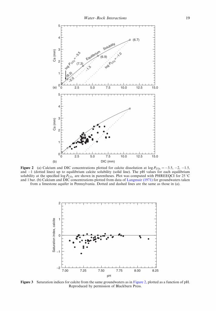
0 2.5 5.0 7.5 10.0 12.5 15.00

1

2

3

4

5

Ca

(mm

)

0 2.5 5.0 7.5 10.0 12.5 15.00

1

2

3

4

5

Ca

(mm

)

log

P CO 2 =

−3.5

log P CO2

= −1.0

–2.0

−1.5

(6.9)Equilib

riumSolubility

(6.7)

(7.3)

(8.3)

(b)

(a)

DIC (mm)

Figure 2 (a) Calcium and DIC concentrations plotted for calcite dissolution at logPCO2¼�3.5, �2, �1.5,

and �1 (dotted lines) up to equilibrium calcite solubility (solid line). The pH values for each equilibriumsolubility at the specified logPCO2

are shown in parentheses. Plot was computed with PHREEQCI for 25 1Cand 1 bar. (b) Calcium and DIC concentrations plotted from data of Langmuir (1971) for groundwaters taken

from a limestone aquifer in Pennsylvania. Dotted and dashed lines are the same as those in (a).

7.00 7.25 7.50 7.75 8.00 8.25

pH

−2

−1

0

1

2

Sat

urat

ion

inde

x, c

alci

te

Figure 3 Saturation indices for calcite from the same groundwaters as in Figure 2, plotted as a function of pH.Reproduced by permission of Blackburn Press.



As the pH increases, there is a greater propor-tion of carbonate ions relative to bicarbonatethat increases the saturation with respectto calcite. At pH values t7, waters are nearlyalways undersaturated with respect to calcite(and most other carbonate minerals).

Pyrite oxidation is a complex hydrobiogeo-chemical processes that accounts for about11% of the sulfate found in river drainages(Berner and Berner, 1996; although these esti-mates do not include large flows of acid minedrainage from Rio Tinto and Odiel Basins tothe ocean, Nieto et al., 2007). Mining activitieshave increased the rate of pyrite oxidation andcaused severe contamination of many water-ways with acid and metals. When pyrite oxi-dizes, the sulfur rapidly converts into sulfatebut the oxidation of the iron proceeds moreslowly, depending on pH. Simulating the oxi-dation of pyrite is instructive in summarizingthe chemistry of this complex process (Nordst-rom, 2000). In Figure 4, PHREEQCI was usedto simulate pyrite oxidation by adding incre-ments of oxygen to pyrite in water. The reac-tion also could be simulated by addingincrements of pyrite to an excess of oxygen.The results vary with the amount of oxidationallowed and are represented in the figure by asolution pH as a function of the amount ofpyrite oxidized. First, pyrite oxidation to anacid ferrous sulfate solution only, is shown bythe solid line. Second, the same reaction occursbut the ferrous iron is allowed to oxidize

10−2 10−1 1

Pyrite oxidize

1

2

3

4

pH

Crossover pH = 3.26

Pyrite oxidized, n

Pyrite oxidized,Fe(II) oxidized, and

ferrihydrite precipitated

Pyrite oxidno

Goethite preci

Figure 4 Change in pH as a function of the amountoxidizes to an acid ferrous sulfate solution without any furesultant ferrous sulfate solution is allowed to oxidize, bupyrite oxidizes, the ferrous sulfate solution oxidizes andline); and (4) pyrite oxidizes, ferrous sulfate solution ox

puted with PHREEQCI at 25 1C and 1 bar; therm

without forming a precipitate, shown by thedashed line with a crossover pH of 3.26. Third,a precipitate such as ferrihydrite is allowed toform, which lowers the crossover pH to 2.39. Ifthe Ksp of the precipitating phase is lower, suchas that for crystalline goethite, the crossoverpH is much lower as shown by the dotted line.However, crystalline goethite is not stable atpH values o2 and jarosite would precipitateinstead. The reason for showing the goethitecurve is to demonstrate the effect of loweringthe Ksp for a precipitating phase of the samestoichiometry. The dashed lines cross over theoriginal line, because the oxidation of ferrousiron involves both proton-consuming and pro-ton-producing reactions. The oxidation ofFe2þ–Fe3þ consumes protons:

Fe2þ14O2 þHþ-Fe3þþ1

2H2O ð17Þ

which happens at all pH values. The hydrolysisand precipitation of a ferric hydroxide phaseproduces protons:

Fe3þ þH2O-FeðOHÞ2þ þHþ ð18Þ

Fe3þþ3H2O-FeðOHÞ3þ3Hþ ð19Þ

which only happens if the pH has reached thepoint of hydrolysis, i.e., near or above apH¼ pK1¼ 2.2 for Fe3þ hydrolysis. Consequently,

101 102 103

d (mmol kg−1 )

Crossover pH = 2.39

o Fe(II) oxidized

ized, Fe(II) oxidized precipitation

pitation

H2O

of pyrite oxidized under four scenarios: (1) pyriterther oxidation (solid line); (2) pyrite oxidizes and thet no precipitation is allowed (upper dashed line); (3)precipitates ferrihydrite (pKsp¼ 4.89, lower dashedidizes, and goethite precipitates (dotted line). Com-odynamic data from Nordstrom et al. (1990).

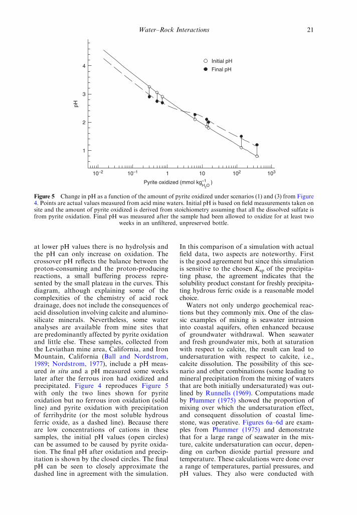
10−2 10–1 1 10 102 103

1

2

3

4

pH

Initial pH

Final pH

Pyrite oxidized (mmol kg–1 )H2O

Figure 5 Change in pH as a function of the amount of pyrite oxidized under scenarios (1) and (3) from Figure4. Points are actual values measured from acid mine waters. Initial pH is based on field measurements taken onsite and the amount of pyrite oxidized is derived from stoichiometry assuming that all the dissolved sulfate isfrom pyrite oxidation. Final pH was measured after the sample had been allowed to oxidize for at least two

weeks in an unfiltered, unpreserved bottle.


at lower pH values there is no hydrolysis andthe pH can only increase on oxidation. Thecrossover pH reflects the balance between theproton-consuming and the proton-producingreactions, a small buffering process repre-sented by the small plateau in the curves. Thisdiagram, although explaining some of thecomplexities of the chemistry of acid rockdrainage, does not include the consequences ofacid dissolution involving calcite and alumino-silicate minerals. Nevertheless, some wateranalyses are available from mine sites thatare predominantly affected by pyrite oxidationand little else. These samples, collected fromthe Leviathan mine area, California, and IronMountain, California (Ball and Nordstrom,1989; Nordstrom, 1977), include a pH meas-ured in situ and a pH measured some weekslater after the ferrous iron had oxidized andprecipitated. Figure 4 reproduces Figure 5with only the two lines shown for pyriteoxidation but no ferrous iron oxidation (solidline) and pyrite oxidation with precipitationof ferrihydrite (or the most soluble hydrousferric oxide, as a dashed line). Because thereare low concentrations of cations in thesesamples, the initial pH values (open circles)can be assumed to be caused by pyrite oxida-tion. The final pH after oxidation and precip-itation is shown by the closed circles. The finalpH can be seen to closely approximate thedashed line in agreement with the simulation.

In this comparison of a simulation with actualfield data, two aspects are noteworthy. Firstis the good agreement but since this simulationis sensitive to the chosen Ksp of the precipita-ting phase, the agreement indicates that thesolubility product constant for freshly precipita-ting hydrous ferric oxide is a reasonable modelchoice.

Waters not only undergo geochemical reac-tions but they commonly mix. One of the clas-sic examples of mixing is seawater intrusioninto coastal aquifers, often enhanced becauseof groundwater withdrawal. When seawaterand fresh groundwater mix, both at saturationwith respect to calcite, the result can lead toundersaturation with respect to calcite, i.e.,calcite dissolution. The possibility of this sce-nario and other combinations (some leading tomineral precipitation from the mixing of watersthat are both initially undersaturated) was out-lined by Runnells (1969). Computations madeby Plummer (1975) showed the proportion ofmixing over which the undersaturation effect,and consequent dissolution of coastal lime-stone, was operative. Figures 6a–6d are exam-ples from Plummer (1975) and demonstratethat for a large range of seawater in the mix-ture, calcite undersaturation can occur, depen-ding on carbon dioxide partial pressure andtemperature. These calculations were done overa range of temperatures, partial pressures, andpH values. They also were conducted with

(a) Percent seawater in mixture

1.0

0.8

0.6

0.4

0.2

0.0

−0.2

−0.4

−0.6

−0.8

−1.0

−1.2

−1.4

10 20 30 40 50 60 70 80 90 1000

Cal

cite

sat

urat

ion

inde

x

Supersaturation

10−4.0 atm

10−3.0 atm

10−2.0 atm

1 atm

Undersaturation10−1.0 atm

(b) Percent seawater in mixture

1.0

0.8

0.6

0.4

0.2

0.0

−0.2

−0.4

−0.6

−0.8

−1.0

−1.2

−1.4

10 20 30 40 50 60 70 80 90 1000

Cal

cite

sat

urat

ion

inde

x

Supersaturation10−4.0 atm

10−3.0 atm

10−2.0 atm

1 atm

Undersaturation

10−1.0 atm

Percent seawater in mixture

1.0

0.8

0.6

0.4

0.2

0.0

−0.2

−0.4

−0.6

−0.8

−1.0

−1.2

−1.4

10 20 30 40 50 60 70 80 90 1000

Cal

cite

sat

urat

ion

inde

x

Supersaturation

10−4.0

10−3.0

10−2.0 atm

10−4.0 atm

1 atm

Undersaturation

10−1.0 atm

(c) Percent seawater in mixture

1.0

0.8

0.6

0.4

0.2

0.0

−0.2

−0.4

−0.6

−0.8

−1.0

−1.2

−1.4

10 20 30 40 50 60 70 80 90 1000

Cal

cite

sat

urat

ion

inde

x

Supersaturation

10−3.010−3.0

10−2.0 atm

10−4.0 atm

1 atm

Undersaturation

10−1.0 atm

(d)

5 °C 15 °C

25 °C 35 °C

10−1.0

atm

Figure 6 Calcite saturation indices plotted as a function of percent seawater mixing with a carbonate aquiferwater with contours representing different levels of PCO2

. Source: Plummer (1975).


actual carbonate groundwater compositionsand coastal seawater for several locations alongthe Florida coast.

The inverse or mass-balance modeling ap-proach provides additional constraints on re-actant and product mineral phases when themineral mass transfers are plotted as a functionof the range of solid solution compositions.Bowser and Jones (2002) (Chapter 5.04)discovered this application when investigatingthe effect of compositional ranges of feld-spars, phyllosilicates, and amphiboles on mass

balances for catchments and groundwatersdominated by silicate hydrolysis. They investi-gated nine drainages in six areas of widelyvarying lithology and climatic settings in theUnited States. One of these is shown in Figure 7for the Wyman Creek drainage in the InyoMountains, California. Mineral mass transfersfor dissolution (positive values in mol kg–1) andprecipitation (negative values in mol kg–1) areplotted as a function of the percent montmo-rillonite solid solution. The gray band shows therestricted range of solid solution composition

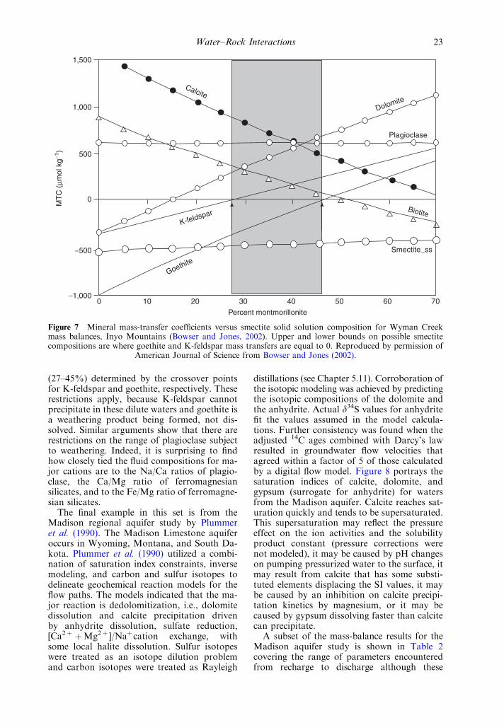
1,500

1,000

500

0

−500

−1,000

Percent montmorillonite

MT

C (

µmol

kg−1

)

Dolomite

Plagioclase

Biotite

Smectite_ss

Goethite

K-feldspar

Calcite

0 10 20 30 40 50 60 70

Figure 7 Mineral mass-transfer coefficients versus smectite solid solution composition for Wyman Creekmass balances, Inyo Mountains (Bowser and Jones, 2002). Upper and lower bounds on possible smectitecompositions are where goethite and K-feldspar mass transfers are equal to 0. Reproduced by permission of

American Journal of Science from Bowser and Jones (2002).


(27–45%) determined by the crossover pointsfor K-feldspar and goethite, respectively. Theserestrictions apply, because K-feldspar cannotprecipitate in these dilute waters and goethite isa weathering product being formed, not dis-solved. Similar arguments show that there arerestrictions on the range of plagioclase subjectto weathering. Indeed, it is surprising to findhow closely tied the fluid compositions for ma-jor cations are to the Na/Ca ratios of plagio-clase, the Ca/Mg ratio of ferromagnesiansilicates, and to the Fe/Mg ratio of ferromagne-sian silicates.

The final example in this set is from theMadison regional aquifer study by Plummeret al. (1990). The Madison Limestone aquiferoccurs in Wyoming, Montana, and South Da-kota. Plummer et al. (1990) utilized a combi-nation of saturation index constraints, inversemodeling, and carbon and sulfur isotopes todelineate geochemical reaction models for theflow paths. The models indicated that the ma-jor reaction is dedolomitization, i.e., dolomitedissolution and calcite precipitation drivenby anhydrite dissolution, sulfate reduction,[Ca2þ þMg2þ ]/Naþcation exchange, withsome local halite dissolution. Sulfur isotopeswere treated as an isotope dilution problemand carbon isotopes were treated as Rayleigh

distillations (see Chapter 5.11). Corroboration ofthe isotopic modeling was achieved by predictingthe isotopic compositions of the dolomite andthe anhydrite. Actual d34S values for anhydritefit the values assumed in the model calcula-tions. Further consistency was found when theadjusted 14C ages combined with Darcy’s lawresulted in groundwater flow velocities thatagreed within a factor of 5 of those calculatedby a digital flow model. Figure 8 portrays thesaturation indices of calcite, dolomite, andgypsum (surrogate for anhydrite) for watersfrom the Madison aquifer. Calcite reaches sat-uration quickly and tends to be supersaturated.This supersaturation may reflect the pressureeffect on the ion activities and the solubilityproduct constant (pressure corrections werenot modeled), it may be caused by pH changeson pumping pressurized water to the surface, itmay result from calcite that has some substi-tuted elements displacing the SI values, it maybe caused by an inhibition on calcite precipi-tation kinetics by magnesium, or it may becaused by gypsum dissolving faster than calcitecan precipitate.

A subset of the mass-balance results for theMadison aquifer study is shown in Table 2covering the range of parameters encounteredfrom recharge to discharge although these

1.0

0.5

0

−0.5

−1.00 5 10 15 20 25

0

−1

−2

−3

Gyp

sum

sat

urat

ion

inde

xD

olom

ite s

atur

atio

n in

dex

Cal

cite

sat

urat

ion

inde

x

1.0

0.5

0

−0.5

−1.0

−1.5

−2.00 5 10 15 20 25

0 5 10 15 20 25

Sulfate concentration (mmol kg−1 )H2O

Figure 8 Saturation indices for calcite, dolomite, and gypsum for groundwaters from the Madison limestoneaquifer. Source: Plummer et al. (1990).


selected samples are not along the same flowpath. The general trend in chemistry is indicatedhere. Samples near recharge are low in sulfateand the amount of mass transfer is low. As thewater moves down gradient and evolves chem-ically, it increases in sulfate from anhydrite dis-solution. Increased anhydrite dissolution leadsto increased dissolution of dolomite and in-creased calcite precipitation. With increasingage there is more organic matter (represented byCH2O in Table 2) available for decomposition,which results in greater amounts of hydrousferric oxides dissolving (reducing) and pyrite

being formed. Cation exhange in Table 2 refersto (CaþMg)/Na, i.e., exchange of calcium andmagnesium for sodium. The measured sulfurisotopic compositions of the H2S and of theanhydrite match nicely with the model simula-tion and the stable carbon isotopes.

Mazor et al. (1993) pointed out that some ofthe samples from the Madison aquifer had hightritium contents when the 14C results indicateddates too old for tritium and suggested thatsignificant mixing of younger and older watersmay have occurred. Mixing and dilution trendscan have similar chemical appearances to

Table 2 Selected mass transfer (in mmol kg�1 water) results from Plummer et al. (1990) for the MadisonLimestone aquifer.

Well no. F6-19 F6-17 F6-13 F7-10 F8-25 F8-21 F3-20

SO4 0.18 0.52 2.19 5.73 8.97 13.56 19.86Dolomite 0.14 0.14 0.60 0.74 1.87 2.90 3.54Calcite �0.18 �0.41 �1.62 �2.64 �4.70 �7.15 �5.33Anhydrite 0.15 0.51 2.27 5.93 9.19 13.56 20.15CH2O 0.01 0.02 0.20 0.44 0.71 0.30 0.87FeOOH 0.00 0.01 0.05 0.12 0.21 0.11 0.09Pyrite �0.00 �0.01 �0.05 �0.12 �0.19 �0.06 �0.09Ion exch. 0.01 0.03 0.04 0.44 0.19 0.14 8.28NaCl �0.01 �0.02 0.03 2.83 1.38 0.97 15.31KCl 0.01 0.02 0.02 0.27 0.28 0.33 2.52CO2 �0.07 0.17 –0.21 �0.42 �1.18 �0.40 �0.04d13C (%) calculated �8.86 �9.33 �7.79 �9.67 �5.52 �3.59 �2.21D13C (%) measured �7.82 �10.0 �6.80 �9.70 �5.50 �3.50 �2.34Apparent age (years) Modern Modern Modern 2,386 14,461 13,310 22,588

Note: Positive values signify dissolution and negative values precipitation. Samples, although not along the same flow path, are in the generaldirection of recharge to discharge from left to right.


hydrochemical evolution, and caution must beused to distinguish evolutionary trends frommixing trends by age-dating techniques.

5.02.8.4 Reactive-Transport Modeling inStreams

Although biological reactions, mostly dis-solved oxygen degradation or nutrient uptake,have been modeled in flowing streams andrivers for a long time, trace-metal reactionshave not been modeled until relatively recently.Bencala (1983) considered solute transport inpool-and-riffle streams using a kinetic term forsorption; and Bencala and Walters (1983) in-troduced transient storage into their modelingof trace-metal transport. One of the mostobvious inputs of trace metals to surface wa-ters is from mining and mineral-processingwastes. Techniques for modeling these acidmine water reactions continued to developduring the 1990s from empirical rate constantsand partition coefficients to mechanistic sorpt-ion models such as surface complexation andequilibrium precipitation of mineral phases(Brown and Hosseinipour, 1991; Kimballet al., 1994, 1995; Runkel et al., 1996, 1999).Reaction-transport models such as these re-quire more accurate stream-discharge measure-ments than can be obtained from current-metermeasurements. These are obtained from con-stant-flow tracer injection studies along withsynoptic sampling, including all possible in-flows, so that the transport model can be re-liably calibrated. Not only has this approachbeen used to define sources and sinks of tracemetals in mountainous streams but it also hasbeen helpful in predicting remediation scenar-ios for mine sites (Runkel and Kimball, 2002).

An example of modeling reactive transportof acid mine waters with OTEQ is shown inFigure 9 (Ball et al., 2003) for the drainagereleased from the Summitville mine in the SanJuan Mountains of southwestern Coloradointo the Alamosa River. The model was cali-brated with tracer injection and synoptic sa-mpling techniques including measurements ofFe(II/III) that helped constrain precipitation ofhydrous ferric oxides in the model. Sodiumchloride was used as the tracer. Figure 9ashows measured pH and simulated pH withreaction. The main in-stream reactive chemistryin this system is the oxidation of iron, the pre-cipitation of hydrous ferric oxides, the precip-itation of hydrous aluminum oxides, theadsorption of trace metals, and pH changes(controlled by the oxidation, hydrolysis, andprecipitation reactions and by the neutraliza-tion of inflows). Simulated and measureddissolved and total aluminum and ironconcentrations are shown in Figures 9b and9c, respectively. Iron and aluminum concentra-tions decrease rapidly because of precipitationduring downstream transport. Figure 9d showsthe copper concentrations; when adsorption isinvoked in the model the agreement betweenmeasured and simulated copper concentrationsis within analytical error.

5.02.8.5 Geochemical Modeling of Catchments

Attempts to model chemical weathering ofcatchments have used a variety of approachesand were originally designed to understandacidification processes. The BIRKENES code(Christophersen et al., 1982) was one of the firstdeveloped to model catchment stream chemis-try. It used cation–anion charge balance, a

8

7

6

5

4

30 5 10 15 20 25 30

Wightman Forkat mouth

Alamosa River TerraceReservoir

pH (

stan

dard

uni

ts)

(a)

300

250

200

150

100

50

0

0 5 10 15 20 25 30


Alamosa RiverTerrace

Reservoir

Al (

µm)

(b)

250

200

150

100

50

0

(c)

0 5 10 15 20 25 30

TerraceReservoirAlamosa River


25

20

15

10

5

00 5 10 15 20 25 30

Distance (km)


Alamosa River

TerraceReservoir

Dissolved Total

SimulatedMeasured

Fe

(µm

)

Cu

(µm

)

(d)

Figure 9 Downstream profiles in the Wightman Fork/Alamosa River system of: (a) pH measured andsimulated; (b) dissolved aluminum concentrations measured and simulated; (c) dissolved iron concentrationsmeasured and simulated; and (d) copper concentrations measured and simulated. Simulations were obtained

with the OTEQ code after calibration on tracer-injection data and Fe(II/III) determinations.



gibbsite equilibrium solubility control for al-uminum concentrations, a Gapon ion exchangefor metals sorption, and rates for sulfate ad-sorption/desorption in a two-reservoir model.The model was calibrated by input mass fluxesand output mass fluxes for the Birkenes catch-ment in Norway to provide the water flux in-formation and to fit empirical parameters.

The ILWAS code (Integrated Lake-Water-shed Acidification Study; Chen et al., 1983;Gherini et al., 1985) also contains a semi-empirical model but is much more detailed thanthe BIRKENES code with respect to itshydrologic and geochemical compartments.Alkalinity was one of the key chemical com-ponents in the model. Because the code wasoriginally calibrated on three watersheds re-ceiving acid rain in upstate New York, it wasprogrammed with mineral rate dissolutiondata, gibbsite solubility equilibrium, and otherparameters pertinent to those environments.The considerable quantity of detailed dataneeded to calibrate the ILWAS code limits itsgeneral usefulness.

The MAGIC code (Model of Acidification ofGroundwater In Catchments; Cosby et al.,1985a, b) is similar in many respectsto the BIRKENES code, but parameters forsoil–water and stream–water chemistry are‘‘lumped’’ or averaged over the spatial scalethat can include many heterogeneities. MAGICwas designed to simulate long-term (annual)averages, whereas BIRKENES was designed tosimulate short-term (hours to days) responses.Equilibrium reactions include soil cation-exchange reactions, solubility control bygibbsite, CO2–H2O hydrolysis reactions, aque-ous speciation of aluminum among sulfateand fluoride complexes, water dissociation,ion balance, and temperature dependence.Activity coefficients appear not to have beenused and the sensitivity of the model to thisfactor has not been addressed. Wright andCosby (1987) found good agreement betweensimulated and measured alkalinities for twomanipulated catchments in Norway using theMAGIC code. Organic acids have been in-cluded with the code and the simulations of theNorway catchments revisited with improvedresults (Cosby et al., 1995). An alternative toILWAS and MAGIC is the code EnhancedTrickle Down (ETD; Nikolaidis et al., 1989,1991). Geochemical processes include cationexchange, chemical weathering, sulfate adsorp-tion, and sulfate reduction. Comparisons of thethree codes, ILWAS, MAGIC, and ETD, weremade by Rose et al. (1991a, b). The codes werefound to provide similar forecasts on a relativescale but substantial differences with respectto specific concentrations (absolute scale).

Codes that contain more detailed considera-tion of chemistry, especially reaction kinetics,include PROFILE (Sverdrup, 1990; Warfvingeand Sverdrup, 1992) and UNSATCHEM (forthe unsaturated zone, Suarez and Simunek,1996).

The main problem with any of these modelsis that they are calibrated with data that are tooshort-term for the long-term processes they aretrying to predict on the catchment scale(Drever, 1997b; Hornberger, 2002).

5.02.8.6 Reliability of Geochemical ModelSimulations

One approach to determine the reliability ofgeochemical codes is to take well-defined inputdata and compare the output from several dif-ferent codes. For comparison of speciation re-sults, Nordstrom et al. (1979) compiled aseawater and a river water test case, that is,seawater and river water analyses that wereused as input to 14 different codes. The resultswere compared and contrasted, demonstratingthat the thermodynamic databases, the numberof ion pairs and complexes, the form of theactivity coefficients, the assumptions made forredox species, and the assumptions made forequilibrium solubilities of mineral phases wereprominent factors in the results. Additional ar-senic, selenium, and uranium redox test caseswere designed for testing of the WATEQ4Fcode (Ball and Nordstrom, 1991). Broyd et al.(1985) used a groundwater test case and com-pared the results from 10 different codes. Suchtest cases could be expanded to include exam-ples of heterogeneous reactions, mixing withreaction, sorption, temperture dependence, re-active transport, and inverse modeling. Thecurrent version of PHREEQC includes 18 ex-amples of code testing. Some of these are true‘‘tests’’ in that they can be compared withmeasurements or independent computations,while others are just examples of the code ca-pability. The EQ3/6 code also shows severalexamples of code capability in addition tocomparative tests. A comparison of PHREEQCand HYDROGEOCHEM codes to simulatetransport and reaction of acidic fluids inalluvial material was obtained by Brown et al.(2000). This comparison gave similar resultsand differences were attributed to differentunits in model output, different activity coef-ficient expressions, and different ionic-strengthcalculations. The equilibrium assumptions usedby the codes did not appear to hold for columnleaching studies.

In another example, five test cases were com-puted by PHREEQE and EQ3/6 and the same


thermodynamic database was run for eachprogram (INTERA, 1983) to test for any codedifferences. The five examples were speciation ofseawater with major ions, speciation of seawaterwith complete analysis, dissolution of microclinein dilute HCl, reduction of hematite and calciteby titration with methane, and dedolomitizationwith gypsum dissolution and increasing temper-ature. The results were nearly identical for eachtest case. Test cases need to become standardpractice when using geochemical codes so thatthe results will have better credibility. A com-parison of code computations with experimentaldata on activity coefficients and mineral sol-ubilities over a range of conditions will also im-prove credibility (Nordstrom, 1994).

Bruno et al. (2002) compared the results ofblind-prediction modeling for geochemicalmodeling of several trace elements of concernto radioactive waste disposal for six naturalanalog sites. Blind-prediction modeling was anexercise developed in radioactive research onrepository analog sites whereby actual wateranalyses for major ions were given to differentgroups of geochemical modelers who wereasked to simulate dissolved trace-element con-centrations based on assumed solubility equili-bria; the results were compared with actualtrace-element concentrations determined on thegroundwaters but kept secret from the model-ers until the modeling was completed. Theyfound that thorium and uranium seem to becontrolled by mineral solubilities, whereasstrontium, zinc, and rare earth element (REE)mobilities seem to be related to the major ionsand complex formation. Other elements such asnickel suffer from insufficient thermodynamicdata. Sorption reactions were not examined insufficient detail to draw conclusions.

Another approach to determining model re-liability is to perform sensitivity or uncertaintyanalyses. One of the first examples is the exam-ination of equilibrium aluminum computationsfor surface waters using the Monte Carlomethod of randomizing sources of error in thewater analysis and thermodynamic data (Schec-her and Driscoll, 1987, 1988). The resultsshowed that uncertainties in the input data didnot contribute significantly to computationalspeciation errors. Nordstrom and Ball (1989)used two different sets of water analyses,groundwater analyses from a granite in Swe-den, and surface water analyses from a creekreceiving AMD in California, to evaluate un-certainties in the water analyses and uncertain-ties in the thermodynamic data as possiblesources of consistent supersaturation effects forcalcite, fluorite, barite, ferric oxyhydroxide, andaluminum hydroxide. Instead of Monte Carlomethods, they used a brute force approach and

recomputed the speciation assuming reasonableerrors in the input analytical data and in thethermodynamic data. The conclusion was thatsupersaturation for these minerals could not beaccounted for by errors in the water analysesnor in the thermodynamic data. For ferric oxy-hydroxide, iron colloids were probably gettingthrough the filter and contributing to the ap-parent dissolved Fe(iii) concentrations and thesupersaturation effect. For aluminum hydrox-ide, the saturation indices did not indicatesupersaturation with respect to amorphousaluminum hydroxide and hence they were prob-ably reasonable. For the remaining minerals itwas concluded that the supersaturation mayhave been realistic, because it could not be ac-counted for by propagation of these errors.Other causes of supersaturation include impuremineral phases (solid substitution or defects),disordered or fine-grained nature, inhibition ofprecipitation rates, and possible unaccountedfor pressure effects on equilibria.

Criscenti et al. (1996) determined overall un-certainty from geochemical computations by acombination of propagating Monte-Carlo-generated analytical and thermodynamic un-certainties through a geochemical code andapplying the ‘‘generalized sensitivity analysis’’(Spear and Hornberger, 1980) to the output.One of the results of this study is that theaqueous speciation scheme used in many geo-chemical codes is not necessarily consistentwith the speciation scheme used to definestandard pH buffers by the National Bureauof Standards. This conclusion raises the possi-bility that geochemical computations introducean error when speciating natural water basedon a field pH measurement calibrated with oneof these buffers. Cabaniss (1999) investigatedmethods of uncertainty propagation, com-paring the derivative-based method (assumesa linear approximation) with the Monte Carlotechnique for solubility equilibria computa-tions of gibbsite, calcite, and jarosite. He foundthat derivative methods and the assumption ofGaussian uncertainty can misrepresent thepropagated uncertainty.

Computational speciation can be comparedwith analytical speciation for some species.There is always the problem that analyticalmethods also suffer from operational defini-tions, interferences, limits of detection, and as-sociated assumptions. Nevertheless, there is nobetter method of determining accuracy ofspeciation than by comparing analytical resultswith computational results (Nordstrom, 1996).In the few instances where this has been done,the comparison ranges from excellent to poor.Examples of studies of this type can be found inLeppard (1983), Batley (1989), and Nordstrom

Final Comments 29

(1996, 2001). Sometimes, comparison of twoanalytical methods for the same speciation cangive spurious results. In Table 3, measured andcalculated ionic activity coefficients for seawa-ter at 25 1C and 35% salinity are compared,after adjusting to a reference value ofgCl¼ 0.666 (Millero, 2001). These values wouldindicate that for a complex saline solution suchas seawater, the activity coefficients can be cal-culated with a high degree of confidence. Muchmore effort along these lines is needed to betterdetermine the errors and uncertainties forspeciation calculations and to identify reactionequilibria and species for which thermodynamic data need to be measured.

Iron redox speciation was evaluated bycomparing the Eh values computed from aspeciation code that accepts Fe(ii) and Fe(iii)

Table 3 Comparison of measured and calculatedion activity coefficients in seawater at 25 1C and 35%salinity, referenced to gCl¼ 0.666 (Millero, 2001).

Ion Measured Calculated

Hþ 0.590 0.592Naþ 0.6680.6700.678 0.674Kþ 0.625 0.619NH4

þ 0.6160.592 0.624Mg2þ 0.2420.22 0.211Ca2þ 0.2030.180 0.205F– 0.296 0.297Cl– 0.666 0.666OH– 0.2420.2540.254 0.263HS– 0.6810.6730.550 0.688HCO3

� 0.5760.5920.528 0.574B(OH)4

� 0.4190.3980.351 0.384SO4

2� 0.1040.1120.1210.121 0.110CO3

2� 0.0400.0410.0350.035 0.041

Leviathan samp

Iron Mountain s

Summitville sam

0 0.2 0.4

Eh calculated

0

0.2

0.4

0.6

0.8

1.0

Eh

(mea

s. P

t ele

ctro

de)

(V)

Figure 10 Eh measured with a Pt electrode on site conations and speciated with WATEQ

concentrations determined analytically with Ehvalues measured electrometrically with a plat-inum electrode. An example of this comparisonis shown in Figure 10 (Nordstrom, 2000). Foriron concentrations greater than 10–6m, thecomparison is generally excellent (usuallywithin 30mV), indicating that the analyticaldata, speciation calculations, and redox meas-urements are all consistent with equilibriumas predicted by the Nernst equation. This com-parison is one of two redox speciation compu-tations that can be tested electrometrically.Deviations from equilibrium are apparent atlow iron concentrations, because the electro-activity of iron is low enough that other elec-tron acceptors, such as dissolved oxygen, beginto interfere. The other redox condition thatpermits testing with the Nernst equation issulfide. Berner (1963) showed that the platinumelectrode gives Nernstian behavior in anoxicmarine sediments in response to dissolvedsulfide activities. All other redox species in nat-ural waters are not sufficiently electroactive toestablish Nernstian equilibrium.

Nordstrom (2001) demonstrated that if onecompares computed free-fluoride ion activitiesor concentrations (in this example, with WA-TEQ4F) with measured values obtained with afluoride ion-selective electrode, the results arein good agreement down to B10–6m. Thisagreement between measurement and calcula-tion corroborates the fluoride speciation by theIA method.

5.02.9 FINAL COMMENTS

Numerous models and codes have beendeveloped over the last century for interpreting

les

amples

ples

0.6 0.8 1.0

from Fe (II/III) (v)

mpared with Eh calculated from Fe(II/III) determi-4F. Source: Nordstrom (2000).


and portraying low-temperature geochemicalprocesses. They have been applied to a greatvariety of conditions and processes and haveenhanced our ability to understand how low-temperature earth systems work. However,many of these models have a dangerous sophis-tication for computing almost any type of pos-sibility without adequately constraining what isprobable. Perhaps this affair is little differentfrom many centuries ago when we had fewerscientific tools and more imagination to playwith. The danger in greater model sophisticationis the difficulty in testing and refuting it. If wecannot test a model, then we have no means ofdetermining its reliability. And yet if we do notstrive for greater sophistication, then the modellacks representativeness (Oreskes, 2000a).

What we must remember is that modelingis a tool—a useful tool to be sure, but notsomething that can ever replace the experiencegained from directly working on a hydrogeo-chemical problem for several years. Expertjudgment, developed over long time periodsand involving many mistakes, along with care-fully acquired empirical observations in thefield and in the laboratory, will ultimately guideour models from possibility to probability.‘‘y even the most mathematically and compu-tationallly sophisticated model will not absolveus of the need for judgment, nor of the needto justify our judgment in human terms’’(Oreskes, 2000a). Expert judgment is particu-larly important in identifying the appropriate-ness of assumptions in applying a model andconstitutes a bigger problem than that of modelformulation.

Model reliability is a very important aspectof communicating computational results tomanagers, risk assessors, stakeholders, politi-cians, and the public. Unfortunately, sophisti-cated model computations are not easy tointerpret, model results are often nonunique,and modeling is often state-of-the-art sciencewhose reliability has not been adequatelytested. Because reliability has often beencouched in terms of ‘‘verification’’ and ‘‘val-idation’’ for the convenience of regulatory re-quirements (Jenne and Krupka, 1984; Jackson,1988; Mattigod, 1995; OECD/NEA, 1994;Kirchner et al., 1996; Huguet, 2001; Freedmanand Ibaraki, 2003; Celia et al., 1992), confusionabout the limitations of models and evenmisunderstandings about how science workshave been propagated. Words such as verifi-cation and validation might make sense ina regulatory or legal setting but are inappro-priate and even incompatible with scientificresearch and the scientific method (Oreskeset al., 1994). Validation is a matter of legiti-macy and has a different context and meaning

than what is sought in science. Evaluation ofmodel capabilities makes scientific sense butnot validation. The question has also beenraised as to whether it is really necessary to‘‘predict’’ in a temporal sense. Scientific pre-diction is better described as ‘‘logical’’ predic-tion not temporal prediction and hangingregulatory decisions solely on the basis ofmodel predictions may not be wise or neces-sary (Oreskes, 2000b).

Science progresses by testing hypotheses andby its explanatory success. Success is measuredby consistency between observations and calcu-lations (which is not proof of validity), logicalstructure, simplicity combined with wide appli-cability, and consensus through independentpeer review (also not proof of validity). Oreskes(2000a) quotes Richard Feynman, ‘‘Doubt is theessence of understanding.’’ Yet doubt is exactlywhat regulatory agencies are trying to minimizeor eliminate. Oreskes (2000a) offers a solutionthat seems obvious to Earth scientists: our com-putational process has far exceeded ourobservational data on natural systems. Morefield data and related empirical observations areneeded. Field data will provide the necessaryconstraints to achieve the legitimacy that isbeing sought by the public. Sophisticated com-putations, especially in the hands of the un-skilled, have the possibility of achieving anypreconceived result unless adequately con-strained by empirical data.

Future efforts should be directed towarddeveloping standardized test cases for a widevariety of processes against which code per-formance can be compared and tested, incorpo-ration of reliable methods of accounting formetal–organic complexing involving humic sub-stances, recognition of artifacts of sample col-lection in the determination of trace elements innatural waters, more comparisons of analyticalversus computed speciation to obtain accuracyestimates of aqueous speciation, development ofroutine techniques for estimating uncertaintiesin model calculations, and more detailed studiesof fine-grained mineralogy that are reactivephases in geochemical systems.

ACKNOWLEDGMENTS

This chapter was accomplished through thesupport of the National Research Program andit has benefited substantially from the hosts ofgeochemical modelers who have brought thestate of the art to its present status. The authoris grateful for the reviews and editing of RobLee and Tim Drever, who properly questionedwriting misdemeanors and awkward styles.

References 31

REFERENCES

Aagard P. and Helgeson H. C. (1982) Thermodynamic andkinetic constraints on reaction rates among minerals andaqueous solutions. Part I: Theoretical considerations.Am. J. Sci. 282, 237–285.

Allison J. D., Brown D. S., and Novo-Gradac K. J. (1991)MINTEQA2/PRODEFA2, A Geochemical AssessmentModel for Environmental Systems, Version 3.0 User’sManual. US Environ. Prot. Agency (EPA/600/3-91/021).

Alpers C. N. and Nordstrom D. K. (1999) Geochemicalmodelling of water–rock interactions in miningenvironments. In Reviews in Economic Geology, vol. 6A,The Environmental Geochemistry of Mineral Deposits:Part A. Processes, Methods and Health Issues (eds. G. S.Plumlee and M. J. Logsdon). Soc. Econ. Geol. Littleton,CO, pp. 289–324.

Alpers C. N., Nordstrom D. K., and Burchard J. M. (1992)Compilation and Interpretation of Water Quality and Dis-charge Data for Acid Mine Waters at Iron Mountain,Shasta County, California, 1940–91. US Geol. Surv. Wa-ter-Resour. Invest. Report 91-4160, 173pp.

Appelo C. A. J. and Postma D. (1993) Geochemistry,Groundwater, and Pollution. A. A. Balkema, Rotterdam,536pp.

Archer D. G. and Nordstrom D. K. (2003) Thermody-namic properties of some arsenic compounds of importto groundwater and other applications. J. Chem. Eng.Data (accepted by journal, but indefinitely suspended byNIST).

Bain J. G., Blowes D. W., Robertson W. D., and Frind E.O. (2000) Modelling of sulfide oxidation with reactivetransport at a mine drainage site. J. Contamin. Hydrol.41, 23–47.

Bain J. G., Mayer K. U., Blowes D. W., Frind E. O.,Molson J. W. H., Kahnt R., and Jenk U. (2001) Mod-elling the closure-related geochemical evolution ofgroundwater at a former uranium mine. J. Contamin.Hydrol. 52, 109–135.

Ball J. W., Jenne E. A., and Cantrell M. W. (1981)WATEQ3—A Geochemical Model with Uranium Added.US Geol. Surv. Open-File Report 81-1183, 81pp.

Ball J. W. and Nordstrom D. K. (1989) Final RevisedAnalyses of Major and Trace Elements from Acid MineWaters in the Leviathan Mine Drainage Basin, Californiaand Nevada—October, 1981 to October, 1982. US Geol.Surv. Water-Resour. Invest. Report 89-4138, 49pp.

Ball J. W. and Nordstrom D. K. (1991) User’s Manual forWATEQ4F, with Revised Thermodynamic Data Base andTest Cases for Calculating Speciation of Major, Trace,and Redox Elements in Natural Waters. US Geol. Surv.Open-File Report 91-183, 189pp.

Ball J. W. and Nordstrom D. K. (1998) Critical evaluationand selection of standard state thermodynamic proper-ties for chromium metal and its aqueous ions, hydrolysisspecies, oxides, and hydroxides. J. Chem. Eng. Data 43,895–918.

Ball J. W., Parks G. A., Haas J. L., Jr., and Nordstrom D.K. (1988) A Personal Computer Version of PHAS20, forthe Simultaneous Multiple Regression of ThermochemicalData. US Geol. Surv. Open-File Report 88-489-A,119pp.

Ball J. W., Runkel R. L. and Nordstrom D. K. (2003)Evaluating remedial alternatives for the Alamosa Riverand Wightman Fork, Summitville, Colorado: applicationof a reactive-transport model to low- and high-flow syn-optic studies (ed. P. Zanetti), Environ. Sci. Environ. Com-put. vol. 2 (in press).

Barnes H. L. (1967) Geochemistry of Hydrothermal OreDeposits. Holt, Rinehart and Winston, New York,670pp.

Barnes H. L. (1997) Geochemistry of Hydrothermal OreDeposits, 3rd edn. Wiley, New York, 972pp.

Bassett R. L. (1997) Chemical modelling on the bare-rockor forested watershed scale. Hydrol. Proc. 11, 695–718.

Bassett R. L. and Melchior D. C. (1990) Chemical mod-elling of aqueous systems: an overview. In ChemicalModelling of Aqueous Systems II (eds. D. C. Melchiorand R. L. Bassett), Symp. Ser. Am. Chem. Soc.,Washington, DC, vol. 416, pp. 1–14.

Batley G. E. (1989) Trace Element Speciation: AnalyticalMethods and Problems. CRC Press, Boca Raton, FL,350pp.

Baverman C., Stromberg B., Moreno L., and Neretnieks I.(1999) CHEMFRONTS: a coupled geochemical andtransport tool. J. Contamin. Hydrol. 36, 333–351.

Bencala K. E. (1983) Simulation of solute transport in amountain pool-and-riffle stream with a kinetic masstransfer model for sorption. Water Resour. Res. 19, 732–738.

Bencala K. E. and Walters R. A. (1983) Simulation of sol-ute transport in a mountain pool-and-riffle stream: atransient storage model. Water Resour. Res. 19, 718–724.

Berner E. K. and Berner R. A. (1996) Global Environment:Water, Air, and Geochemical Cycles. Prentice-Hall,Englewood Cliffs, NJ, 376pp.

Berner R. A. (1963) Electrode studies of hydrogen sulfide inmarine sediments. Geochim. Cosmochim. Acta 27, 563–575.

Berner R. A. (1978) Rate control of mineral dissolutionunder earth surface conditions. Am. J. Sci. 278, 1235–1252.

Bethke C. M. (1994) The Geochemist’s Workbencht Version2.0: A User’s Guide to Rxn, Act2. Tact, React, and Gtplot.University of Illinois, Urbana, 213pp.

Bethke C. M. (1996) Geochemical Reaction Modelling:Concepts and Applications. Oxford University Press, NewYork, 397pp.

Bjerrum J. (1950) On the tendency of metal ions towardcomplex formation. Chem. Rev. 46, 381–402.

Bormann F. H. and Likens G. E. (1967) Nutrient cycling.Science 155, 424–429.

Bowser C. J. and Jones B. F. (1990) Geochemical con-straints on ground waters dominated by silicate hydrol-ysis: an interactive spreadsheet, mass balance approach.Chem. Geol. 84, 33–35.

Bowser C. J. and Jones B. F. (2002) Mineralogic controlson the composition of natural waters dominated by sil-icate hydrolysis. Am. J. Sci. 302, 582–662.

Brown J. G., Bassett R. L., and Glynn P. D. (2000) Re-active transport of metal contaminants in alluvium—model comparison and column simulation. Appl. Geo-chem. 15, 35–49.

Brown K. P. and Hosseinipour E. Z. (1991) New methodsfor modelling the transport of metals from mineral proc-essing wastes into surface waters. J. Environ. Sci. HealthA 26, 157–203.

Broyd T. W., Grant M. M., and Cross J. E. (1985) A Reporton Intercomparison Studies of Computer Programs whichRespectively Model: (i) Radionuclide Migration (ii) Equi-librium Chemistry of Groundwater. EUR 10231 EN, Com-mission of the European Communities, Luxembourg.

Brønsted J. N. (1922) Studies on solubility. Part IV: Theprinciple of specific interaction of ions. J. Am. Chem.Soc. 44, 877–898.

Bruno J., Duro L., and Grive M. (2002) The applicabilityand limitations of thermodynamic geochemical models tosimulate trace element behaviour in natural waters: les-sons learned from natural analogue studies. Chem. Geol.190, 371–393.

Cabaniss S. E. (1999) Uncertainty propagation in geo-chemical calculations: non-linearity in solubility equili-bria. Appl. Geochem. 14, 255–262.

Celia M. A., Gray W. G., Hassanizadeh S. M., and CarreraJ. (eds.) (1992) Validation of geo-hydrological models:Part I. Adv. Water Resour. 15, 1–274.


Charlton S. R., Macklin C. L., and Parkhurst D. L. (1997)PHREEQCI—A Graphical User Interface for the Geo-chemical Computer Program PHREEQC. US Geol. Surv.Water-Resour. Invest. Report 97-4222, 9pp.

Chase M. W., Jr. (ed.) (1998) NIST-JANAF ThermochemicalTables, 4th edn. J. Phys. Chem. Ref. Data, Monograph 9,Parts I and II, 1963pp.

Chemical Modeling of Acid Waters, http://wwwbrr.cr.usgs.gov/projects/GWC chemtherm/software.htm and-/thermo.htm (accessed August 2006).

Chen C. W., Gherini S. A., and Goldstein R. A. (1983) TheIntegrated Lake-Watershed Acidification Study, Vol. 1:Model Principles and Application Procedures. EPRIReport EA-3221.

Christophersen N., Seip H. M., and Wright R. F. (1982) Amodel for streamwater chemistry at Birkenes, Norway.Water Resour. Res. 18, 977–996.

Cosby B. J., Hornberger G. M., Galloway J. N., and WrightR. F. (1985a) Modelling the effects of acid deposition: as-sessment of a lumped-parameter model of soil water andstreamwater chemistry. Water Resour. Res. 21, 51–63.

Cosby B. J., Hornberger G. M., Galloway J. N., andWright R. F. (1985b) Time scales of catchment acidifi-cation. Environ. Sci. Technol. 19, 1144–1149.

Cosby B. J., Wright R. F., and Gjessing E. (1995) Anacidification model (MAGIC) with organic acids evalu-ated using whole-catchment manipulations in Norway.J. Hydrol. 170, 101–122.

Cox J. D., Wagman D. D., and Medvedev V. A. (1989)CODATA Key Values for Thermodynamics. HemispherePublishing Corp, Washington, DC, 271pp.

Criscenti L. J., Laniak G. F., and Erikson R. L. (1996)Propagation of uncertainty through geochemical codecalculations. Geochim. Cosmochim. Acta 60, 3551–3568.

Davis J. A. and Hayes K. F. (1986) In Geochemical Proc-esses at Mineral Surfaces, Am. Chem. Soc. Symp. Series.American Chemical Society, Washington, DC, vol. 323,683pp.

Debye P. and Huckel E. (1923) On the theory of electro-lytes. Phys. Z. 24, 185–208, 305–325.

Derry G. N. (1999) What Science is and How it Works.Princeton University Press, Princeton, NJ, 311pp.

Dobbs J. C., Susetyo W., Carreira L. A., and Azarraga L.V. (1989) Competitive binding of protons and metal ionsin humic substances by lanthanide ion probe spectros-copy. Anal. Chem. 61, 1519–1524.

Domenico P. A. and Schwartz F. W. (1990) Physical andChemical Hydrogeology. Wiley, New York, 824pp.

Drever J. I. (1997a) The Geochemistry of Natural Waters:Surface and Groundwater Environments, 3rd edn. Pren-tice-Hall, Englewood Cliffs, NJ, 436pp.

Drever J. I. (1997b) Catchment mass balance. In Geochem-ical Processes, Weathering, and Groundwater Rechargein Catchments (eds. O. Saether and P. de Cariat). A. A.Balkema, Rotterdam, pp. 241–261.

Dyrssen D., Jagner D., and Wengelin F. (1968) ComputerCalculations of Ionic Equilibria and Titration Procedures.Almqvist and Wiksell, Stockholm, 250pp.

Dzombak D. A. and Morel F. M. M. (1990) Surface Com-plexation Modelling: Hydrous Ferric Oxide. Wiley, NewYork, 393pp.

Eugster H. P. (1971) The beginnings of experimental pet-rology. Science 173, 481–489.

Eugster H. P., Harvie C. E., and Weare J. H. (1980) Min-eral equilibria in the six-component seawater system,Na–K–Mg–Ca–SO4–Cl–H2O, at 25 1C. Geochim. Cosmo-chim. Acta 44, 1335–1347.

Felmy A. R., Girvin D. C., and Jenne E. A. (1984) MINT-EQ—A Computer Program for Calculating AqueousGeochemical Equilibria. US Environ. Prot. Agency(EPA-600/3-84-032).

Felmy A. R., Rai D., and Amonette J. E. (1990) Thesolubility of barite and celestite in sodium sulfate:

evaluation of thermodynamic data. J. Sol. Chem. 19,175–185.

Freedman V. L. and Ibaraki M. (2003) Coupled reactivemass transport and fluid flow: issues in model verificat-ion. Adv. Water Resour. 26, 117–127.

Freeze R. A. and Cherry J. A. (1979) Groundwater. Pren-tice-Hall, Englewood Cliffs, NJ, 604pp.

Garrels R. M. (1960) Mineral Equilibria. Harper andBrothers, New York, 254pp.

Garrels R. M. and Christ C. L. (1965) Solutions, Minerals,and Equilibria. Harper and Row, New York, 450pp.

Garrels R. M. and Mackenzie F. T. (1967) Origin of thechemical composition of some springs and lakes. InEquilibrium Concepts in Natural Water Systems (ed. R. F.Gould), Adv. Chem. Series, vol. 67. Am. Chem. Soc.Washington, DC, pp. 222–242.

Garrels R. M. and Thompson M. E. (1962) A chemicalmodel for seawater at 25 1C and one atmosphere totalpressure. Am. J. Sci. 260, 57–66.

Garvin D., Parker V. B., and White H. J. (1987) CODATAThermodynamic Tables—Selections for Some Compoundsof Calcium and Related Mixtures: A Prototype Set ofTables. Hemisphere Publishing Corp., Washington, DC,356pp.

Gerke H. H., Molson J. W., and Frind E. O. (1998) Mod-elling the effect of chemical heterogeneity on acidificationand solute leaching in overburden mine spoils. J. Hydrol.209, 166–185.

Gherini S. A., Mok L., Hudson R. J. M., Davis G. F., ChenC. W., and Goldstein R. A. (1985) The ILWAS model:formulation and application. Water Air Soil Pollut. 26,425–459.

Glynn P. and Brown J. (1996) Reactive transport modellingof acidic metal-contaminated ground water at a site withsparse spatial information. In Reactive Transport in Po-rous Media (eds. P. C. Lichtner, C. I. Steefel, and E. H.Oelkers). Mineralogical Society of America and Geolo-gical Society, Washington, DC, vol. 34, pp. 377–438.

Goldberg E. D. (1954) Marine geochemistry. 1: Chemicalscavengers of the sea. J. Geol. 62, 249–265.

Greenberg J. P. and Møller N. (1989) The prediction ofmineral solubilities in natural waters: a chemical equi-librium model for the Na–K–Ca–Cl–SO4–H2O system tohigh concentrations from 0 to 250 1C. Geochim. Cosmo-chim. Acta 53, 2503–2518.

Greenwood H. (1989) On models and modelling. Can.Mineral. 27, 1–14.

Grenthe I., Fuger J., Konings R. J. M., Lemire R. J.,Muller A. B., Nguyen-Trung C., and Wanner H. (1992)Chemical Thermodynamics of Uranium. Elsevier, Amster-dam, 715pp.

Grenthe I., Plyasunov A. V., and Spahiu K. (1997) Esti-mations of medium effects on thermodynamic data. InModelling in Aquatic Chemistry (eds. I. Grenthe and I.Puigdomenech). Organization for Economic Co-opera-tion and Development/Nuclear energy Agency Publica-tions, Paris, France, pp. 343–444.

Grenthe I. and Puigdomenech I. (1997). Organization forEconomic Co-operation and Development/Nuclear En-ergy Agency Publications, Paris, France, 742pp.

Gryzb K. R. (1995) NOAEM (natural organic anion equi-librium model): a data analysis algorithm for estimatingfunctional properties of dissolved organic matter inaqueous environments. Part I: Ionic component speciat-ion and metal association. Org. Geochem. 23, 379–390.

Guggenheim G. A. (1935) The specific thermodynamicproperties of aqueous solutions of strong electrolytes.Phil. Mag. 19, 588–643.

Guillaumont R., Fanghanel T., Fuger J., Grenthe I., NeckV., Palmer D. A., and Rand M. H. (2003) Update onthe Chemical Thermodynamics of Uranium, Neptunium,Plutonium, Americium, and Technetium. Elsevier, Am-sterdam, 919pp. with CD.

http://wwwbrr.cr.usgs.gov/projects/GWC_chemtherm/software.htm




References 33

Gurvich L. V., Veyts I. V., Alcock C. B., and Iorish V. S.(1993) Thermodynamic Properties of Individual Sub-stances, Parts 1 and 2. CRC Press, Boca Raton, FL,vol. 3, 1120pp.

Haas J. L., Jr. (1974) PHAS20, a Program for SimultaneousMultiple Regression of a Mathematical Model to Thermo-chemical Data. Natl. Tech. Info. Service Report AD-780301, 158pp.

Haas J. L. and Fisher J. R. (1976) Simultaneous evaluationand correlation of thermodynamic data. Am. J. Sci. 276,525–545.

Harned H. S. and Owen B. B. (1958) The Physical Chem-istry of Electrolyte Solutions, 3rd edn. Reinhold, NewYork, 354pp.

Harvie C. E., Eugster H. P., and Weare J. H. (1982) Min-eral equilibria in the six-component seawater system,Na–K–Mg–Ca–SO4–Cl–H2O at 25 1C. Part II: Compo-sition of the saturated solutions. Geochim. Cosmochim.Acta 46, 1603–1618.

Harvie C. E., Greenberg J. P., and Weare J. H. (1987)A chemical equilibrium algorithm for highly non-idealmultiphase systems: free energy minimization. Geochim.Cosmochim. Acta 51, 1045–1057.

Harvie C. E., Møller N., and Weare J. H. (1984) The pre-diction of mineral solubilities in natural waters: the Na–K–Mg–Ca–H–Cl–SO4–OH–HCO3–CO3–CO2–H2O systemto high ionic strengths at 25 1C. Geochim. Cosmochim. Acta48, 723–751.

Harvie C. E. and Weare J. H. (1980) The prediction ofmineral solubilities in natural waters: the Na–K–Mg–Ca–Cl–SO4–H2O system from zero to high concentration at25 1C. Geochim. Cosmochim. Acta 44, 981–997.

Harvie C. E., Weare J. H., Hardie L. A., and Eugster H. P.(1980) Evaporation of seawater: calculated mineral se-quences. Science 208, 498–500.

Helgeson H. C. (1964) Complexing and Hydrothermal OreDeposition. Pergamon, New York, 128pp.

Helgeson H. C. (1967) Thermodynamics of complex disso-ciation in aqueous solution at elevated temperatures. J.Phys. Chem. 71, 3121–3136.

Helgeson H. C. (1968) Evaluation of irreversible reactionsin geochemical processes involving minerals and aqueoussolutions. Part I: Thermodynamic relations. Geochim.Cosmochim. Acta 32, 853–877.

Helgeson H. C. (1969) Thermodynamics of hydrothermalsystems at elevated temperatures and pressures. Am. J.Sci. 167, 729–804.

Helgeson H. C. (1971) Kinetics of mass transfer amongsilicates and aqueous solutions. Geochim. Cosmochim.Acta 35, 421–469.

Helgeson H. C., Brown T. H., Nigrini A., and Jones T. A.(1970) Calculation of mass transfer in geochemical proc-esses involving aqueous solution. Geochim. Cosmochim.Acta 34, 569–592.

Helgeson H. C., Delany J. M., Nesbitt H. W., and Bird D.W. (1978) Summary and critique of the thermodynamicproperties of rock-forming minerals. Am. J. Sci. 278-A,1–229.

Helgeson H. C., Garrels R. M., and Mackenzie F. T. (1969)Evaluation of irreversible reactions in geochemical proc-esses involving minerals and aqueous solutions. II: Appl.Geochim. Cosmochim. Acta 33, 455–481.

Helgeson H. C. and Kirkham D. H. (1974a) Theoreticalprediction of the thermodynamic behavior of aqueouselectrolytes at high pressures and temperatures. Part I:Summary of the thermodynamic/electrostatic propertiesof the solvent. Am. J. Sci. 274, 1089–1198.

Helgeson H. C. and Kirkham D. H. (1974b) Theoreticalprediction of the thermodynamic behavior of aqueouselectrolytes at high pressures and temperatures. Part II:Debye-Huckel parameters for activity coefficients andrelative partial molal properties. Am. J. Sci. 274,1199–1261.

Helgeson H. C. and Kirkham D. H. (1976) Theoreticalprediction of the thermodynamic behavior of aqueouselectrolytes at high pressures and temperatures. Part III:Equation of state for aqueous species at infinite dilution.Am. J. Sci. 276, 97–240.

Helgeson H. C., Kirkham D. H., and Flowers G. C. (1981)Theoretical prediction of the thermodynamic behavior ofaqueous electrolytes at high pressures and temperatures.Part IV: Calculation of activity coefficients and relativepartial moral properties to 600 1C and 5 kb. Am. J. Sci.281, 1249–1516.

Helgeson H. C. and Murphy W. M. (1983) Calculation ofmass transfer as a function of time and surface area ingeochemical processes. Part I: Computational approach.Math. Geol. 15, 109–130.

Helgeson H. C., Murphy W. M., and Aagard P. (1984)Thermodynamic and kinetic constraints on reaction ratesamong minerals and aqueous solutions. Part II: Rateconstants, effective surface area, and the hydrolysis offeldspar. Geochim. Cosmochim. Acta 48, 2405–2432.

Hem J. D. (1959) Study and Interpretation of the ChemicalCharacteristics of Natural Water. US Geol. Surv.Water-Supply Paper 1473, 269pp.

Hem J. D. (1961) Calculation and Use of Ion Activity. USGeological Survey Water-Supply Paper 1535-C.

Hem J. D. and Cropper W. H. (1959) Survey of Ferrous-ferrric Chemical Equilibria and Redox Potentials. USGeological Survey Water-Supply Paper 1459-145A.

Hitchon B., Perkins E. H., and Gunter W. D. (1996)Introduction of Ground Water Geochemistry and SOL-MINEQ.GW.

Hochella M. F. and White A. F. (1990) Mineral–WaterInterface Geochemistry. Rev. Mineral. 23, 1–16.

Hornberger G. M. (2002) Impacts of acidic atmosphericdeposition on the chemical composition of stream waterand soil water. In Environmental Foresight and Models: AManifesto (ed. M. B. Beck). Elsevier, New York, pp.131–145.

Huber C., Filella M., and Town R. M. (2002) Computermodelling of trace metal ion speciation: practical imple-mentation of a linear continuous function for complex-ation by natural organic matter. Comput. Geosci. 28,587–596.

Huguet J. M. (2001) Testing and Validation of NumericalModels of Groundwater Flow, Solute Transport andChemical Reactions in Fractured Granites: A QuantitativeStudy of the Hydrogeological andHydrochemical ImpactProduced. ENRESA Tech. Publ. 06/2001, 253pp.

Hunter K. S., Wang Y., and Van Cappellen P. (1998)Kinetic modelling of microbially-driven redox chemistryof subsurface environments: coupling transport,microbial metabolism and geochemistry. J. Hydrol. 209,53–80.

HYDROGEOCHEM, http://www.scisoftware. com/prod-ucts/hydrogeochem overview/hydrogeochem overview.html (accessed August 2006).

Ingri N., Kakolowicz W., Sillen L. G., and Warnqvist B.(1967) HALTAFALL, a general program for calculatingthe composition of equilibrium mixtures. Talanta 14,1261–1286.

Ingri N. and Sillen L. G. (1962) High-speed computers as asupplement to graphical methods. Part II: Some compu-ter programs for studies of complex formation equilibria.Acta Chem. Scand. 16, 173–191.

INTERA (1983) Geochemical models suitable for perform-ance assessment of nuclear waste storage: comparison ofPHREEQE and EQ3/EQ6. INTERA EnvironmentalConsultants, Inc., ONWI-473, 114pp.

IPAC, http://www.llnl.gov/ipac/technology/software/soft-waretitles/eq36.php (accessed August 2006).

Jackson K. J. (1988) Verification and validation studies ofthe addition of Pitzer’s equations to the EQ3/6 brinemodel. UCRL-53841, 26pp.

http://www.scisoftware.com/products/hydrogeochem_overview/hydrogeochem_overview.html





http://www.llnl.gov/ipac/technology/software/softwaretitles/eq36.php

http://www.llnl.gov/ipac/technology/software/softwaretitles/eq36.php


Jenne E. A. (ed.) (1979) Chemical Modelling of AqueousSystems, Symp. Series, Am. Chem. Soc. Washington,DC, vol. 93, 914pp.

Jenne E. A. and Krupka K. M. (1984) Validation ofGeochemical Models. USNRC Report PNL-SA-12442,9pp.

Johnson J. W., Oelkers E. H., and Helgeson H. C. (1992)SUPCRT92: a software package for calculating thestandard molal thermodynamic properties of minerals,gases, aqueous species, and reactions from 1 to 5,000barsand 01 to 1,000 1C. Comp. Geosci. 18, 899–947.

Judson H. F. (1980) The Search for Solutions. Holt. Rine-hart and Winston, New York, 211pp.

Kharaka Y. K. and Barnes I. (1973) SOLMNEQ: Solution-Mineral Equilibrium Computations. Natl. Tech. Info.Serv. Report PB214-899, 82pp.

Kharaka Y. K., Gunter W. D., Aggarwal P. K., Perkins E.H., and Debraal J. D. (1988) SOLMINEQ. 88:A Com-puter Program for Geochemical Modelling of Water-rockInteractions. US Geol. Surv. Water-Resour. Invest. Re-port 88-4227, 420pp.

Kimball B. A., Broshears R. E., Bencala K. E.,and McKnight D. M. (1994) Coupling of hydrologictransport and chemical reactions in a stream affe-cted by acid mine drainage. Environ. Sci. Tech. 28,2065–2073.

Kimball B. A., Callender E., and Axtmann E. V. (1995)Effects of colloids on metal transport in a river receivingacid mine drainage, Upper Arkansas River, ColoradoUSA. Appl. Geochem. 10, 285–306.

Kimball B. A., Runkel R. L., Walton-Day K., JamborJ. L., Blowes D. W., Ritchie A. I. M. (2003) Use of Field-Scale Experiments and Reactive Transport Modelling toEvaluate Remediation Alternatives in Streams Affected byAcid Mine Drainage, Mineralogical Association ofCanada, Short Course Series, pp. 261–282.

Kipp K. L., Jr. (1987) HST3D—A Computer Code forSimulation of Heat and Solute Transport in Three-Dimensional Ground-Water Flow Systems. US Geol.Surv. Water-Resour. Invest. Report 86-4095, 517pp.

Kipp K. L., Jr. (1998) Guide to the Revised Heat and SoluteTransport Simulator: HST3D. US Geol. Surv. water-Resour. Report 97-4157, 149pp.

Kirchner J. W., Hooper R. P., Kendall C., Neal C., andLeavesley G. (1996) Testing and validating environmen-tal models. Sci. Total Environ. 183, 33–47.

Konikow L. F. and Bredehoeft J. D. (1992) Ground-watermodels cannot be validated. Adv. Water Resour. 15, 75–83.

Krauskopf K. B. (1951) The solubility of gold. Econ. Geol.46, 858–870.

Krauskopf K. B. (1955) Sedimentary deposits of rare metals.Econ. Geol. Fiftieth Anniv. Part I, pp. 411–463.

Krauskopf K. B. (1956) Factors controlling the concen-trations of thirteen rare metals in sea water. Geochim.Cosmochim. Acta 9, 1–32.

Krauskopf K. B. (1967) Introduction to Geochemistry.McGraw-Hill, New York, 721pp.

Lambert I. and Clever H. L. (1992) Alkaline Earth Hydrox-ides in Water and Aqueous Solutions IUPAC SolubilityData Series, Pergamon, Oxford, UK, vol. 52, 365pp.

Langmuir D. (1971) The geochemistry of some carbonateground waters in central Pennsylvania. Geochim. Cosmo-chim. Acta 35, 1023–1045.

Langmuir D. (1997) Aqueous Environmental Geochemistry.Prentice-Hall, New Jersey, 600pp.

Latimer W. M. (1952) The Oxidation State of the Elementsand their Potentials in Aqueous Solution. Prentice-Hall,New York, 392pp.

Lemire R. J., Fuger J., Nitsche H., Potter P., Rand M. H.,Rydberg J., Spahiu K., Sullivan J. C., Ullman W. J.,Vitorge P., and Wanner H. (2001) Chemical Thermody-namics of Neptunium and Plutonium. North-Holland/Elsevier, Amsterdam, 836pp.

Leppard G. G. (1983) Trace Element Speciation in SurfaceWaters and its Ecological Implications, NATO Conf. Se-ries, vol. 6. Plenum, NY, 320pp.

Lewis G. N. and Randall M. (1921) The activity coeffi-cient of strong electrolytes. J. Am. Chem. Soc. 43, 1112–1153.

Lewis G. N. and Randall M. (1923) Thermodynamics andthe Free Energy of Chemical Substances. McGraw-Hill,New York, 653pp.

Lichtner P. C. (1996) Continuum formulation of multi-component-multiphase reactive transport. In ReactiveTransport in Porous Media (eds. P. C. Lichtner, C. I.Steefel, and E. H. Oelkers). Rev. Mineral., MineralogicalSociety of America, Washington, DC, vol. 34, pp. 1–81.

Lichtner P. C. (2001) FLOTRAN Users Manual. LosAlamos National Laboratory Report LA-UR-01-2349,Los Alamos, NM.

Lichtner P. C., Steefel C. I., and Oelkers E. H. (eds.) (1996)Reactive Transport in Porous Media. Rev. Mineral., Min-eralogical Society of America, Washington, DC, vol. 34,pp. 438.

Likens G. E., Bormann F. H., Pierce R. S., Eaton J. S., andJohnson N. M. (1977) Biogeochemistry of a Forested Ec-osystem. Springer, New York, 146pp.

Loeppert R. H., Schwab A. P. and Goldberg S. (1995)Chemical Equilibrium and Reaction Models, Spec. Publ.,vol. 42, Soil Science Society of America, Madison, WI,422pp.

Majzlan J., Navrotsky A., and Neil J. M. (2002) Energeticsof anhydrite, barite, celestine, and anglesite: a high-tem-perature and differential scanning calorimetry study.Geochim. Cosmochim. Acta 66, 1839–1850.

Makers of MINEQLþ MINEQL þ The First Choice inChemical Equilibrium Modeling, http://www.mine-ql.com/ (accessed August 2006).

Mangold D. C. and Tsang C.-F. (1991) A summary ofsubsurface hydrological and hydrochemical models. Rev.Geophys. 29, 51–79.

Marion G. M. (2001) Carbonate mineral solubility at lowtemperatures in the Na–K–Mg–Ca–H–Cl–SO4–OH–HCO3–CO3–CO2–H2O system. Geochim. Cosmochim. Acta65, 1883–1896.

Marion G. M. (2002) A molal-based model for strong acidchemistry at low temperatures (o200 to 298K). Geo-chim. Cosmochim. Acta 66, 2499–2516.

Marion G. M., Catling D. C., and Kargel J. S. (2003)Modeling aqueous ferrous iron chemistry at low temper-atures with application to Mars. Geochim. Cosmochim.Acta 67, 4251–4266.

Marion G. M. and Farren R. E. (1999) Mineral solubilities inthe Na–K–Mg–Ca–Cl–SO4–H2O system: a re-evaluation ofthe sulfate chemistry in the Spencer–Møller–Weare model.Geochim. Cosmochim. Acta 63, 1305–1318.

Martell A. E. and Smith R. M. (1974–1976) Critical Sta-bility Constants: Vol. 1 Amino Acids, Vol. 2 Amines, Vol.3 Other Organic Ligands, Vol. 4 Inorganic Compounds.Plenum, New York, 1636pp.

Mattigod S. V. (1995) Validation of geochemical models. InChemical Equilibrium and Reaction Models, (eds. R. H.Loeppert and A. P. Schwab, and S. Goldberg) Spec. Publ.Soil Science Society of America, Madison, WI, vol. 42,pp. 201–218.

Mayer K. U., Benner S. G., and Blowes D. W. (1999) Thereactive transport model MIN3P: application to acid-mine drainage generation and treatment—Nickel Rimmine site, Sudbury, Ontario. In Mining and Environment1 (eds. D. Goldsack, N. Bezlie, P. Yearwood, and G.Hall). pp. 145–154.

Mayer K. U., Blowes D.W., and Frind E. O. (2003) Advancesin reactive-transport modelling of contaminant release andattenuation from mine-waste deposits (eds. J. L. Jambor,D. W. Blowes, and A. I. M. Ritchie). Mineralogical Asso-ciation of Canada Short Course Series, pp. 283–302.

http://www.mineql.com/

http://www.mineql.com/

References 35

Mazor E., Drever J. I., Finlay J., Huntoon P. W., andLundy D. A. (1993) Hydrochemical implications ofgroundwater mixing: an example from the SouthernLaramie Basin, Wyoming. Water Resour. Res. 29, 193–205.

Melchior D. C. and Bassett R. L. (1990) Chemical Mod-elling of Aqueous Systems: II Symp. Am. Chem. Soc.,Washington, DC, Ser., vol. 416, 556pp.

Millero F. J. (2001) The Physical Chemistry of NaturalWaters. Wiley, New York, 654pp.

Millero F. J. and Pierrot D. (1998) A chemical model fornatural waters. Aqua. Geochem. 4, 153–199.

Millero F. J. and Roy R. (1997) A chemical model for thecarbonate system in natural waters. Croat. Chem. Acta70, 1–38.

Millero F. J. and Schreiber D. R. (1982) Use of the ionpairing model to estimate activity coefficients of the ioniccomponents of natural waters. Am. J. Sci. 282, 1508–1540.

MINTEQA2/PRODEFA2, A Geochemical AssessmentModel for Enviornmental Systems, http://epa.gov/ceam-publ/mmedia/minteq/supple1.pdf (last accessed August2006).

Møller N. (1988) The prediction of mineral solubilities innatural waters: a chemical equilibrium model for the Na–Ca–Cl–SO4–H2O system, to high temperature and con-centration. Geochim. Cosmochim. Acta 52, 821–837.

Møller N., Greenberg J. P., and Weare J. H. (1998) Com-puter modelling for geothermal systems: predicting car-bonate and silica scale formation, CO2 breakout and H2Sexchange. Transport Porous Media 33, 173–204.

Monnin C. (1990) The influence of pressure on the activitycoefficients of the solutes and on the solubility ofminerals in the system Na–Ca–Cl–SO4–H2O to 200 1Cand 1 kbar, and to high NaCl concentration. Geochim.Cosmochim. Acta 52, 821–834.

Monnin C. and Ramboz C. (1996) The anhydrite saturationindex of the ponded brines and the sediment pore watersof the Red Sea deeps. Chem. Geol. 127, 141–159.

Morel F. and Morgan J. J. (1972) A numerical method forcomputing equilibria in aqueous systems. Environ. Sci.Tech. 6, 58–67.

MurphyW. M. and Helgeson H. C. (1987) Thermodynamicand kinetic constraints on reaction rates among mineralsand aqueous solutions. Part III: Activated complexes andthe pH dependence of the rates of feldspar, pyroxene,wollastonite, and olivine hydrolysis. Geochim. Cosmo-chim. Acta 51, 3137–3153.

Murphy W. M., Oelkers E. H., and Lichtner P. C. (1989)Surface reaction versus diffusion control of mineral dis-solution and growth rates in geochemical processes.Chem. Geol. 78, 357–380.

Nieto J. M., Sarmiento A. M., Olias M., Canovas C. R.,Riba I., Kalman J., and Delvalls T. A. (2007) Acid minedrainage in the Tints and Odiel rivers (Iberian PyriteBelt, SW Spain) and bioavailabilty of the transportedmetals to the Huelva Estuary. Environ. Intern. (in press).

Nikolaidis N. P., Muller P. K., Schnoor J. L., and Hu H. L.(1991) Modelling the hydrogeochemical response of astream to acid deposition using the enhanced trickle-down model. Res. J. Water Pollut. Control Feder. 63,220–227.

Nikolaidis N. P., Schnoor J. L., and Geogakakos K. P.(1989) Modelling of long-term lake alkalinity responsesto acid deposition. J. Water Pollut. Control Feder. 61,188–199.

Nordstrom D. K. (1977) Hydrogeochemical and micro-biological factors affecting the heavy metal chemistry ofan acid mine drainage system. PhD Dissertation, Stan-ford University, 210pp.

Nordstrom D. K. (1994) On the evaluation and applicationof geochemical models, Appendix 2. Proc. 5th CEC Nat-ural Analogue Working Group and Alligator RiversAnalogue Project, Toledo, Spain, October 5–19, 1992.EUR 15176 EN, pp. 375–385.

Nordstrom D. K. (1996) Trace metal speciation in naturalwaters: computational vs. analytical. Water Air SoilPollut. 90, 257–267.

Nordstrom D. K. (2000) Advances in the hydrogeochem-istry and microbiology of acid mine waters. Int. Geol.Rev. 42, 499–515.

Nordstrom D. K. (2001) A test of aqueous speciation:measured vs. calculated free fluoride ion activity. Proc.10th Int. Symp. Water–Rock Interaction, WRI-10,Villasimius, Sardinia, July 10–15, 2001 (ed. R. Cidu),pp. 317–320.

Nordstrom D. K. and Archer D. G. (2003) Arsenic ther-modynamic data and environmental geochemistry. InArsenic in Ground Water (eds. A. H. Welch and K. G.Stollenwerk). Kluwer, Boston, MA, pp. 1–25.

Nordstrom D. K. and Ball J. W. (1989) Mineral saturationstates in natural waters and their sensitivity to thermo-dynamic and analytic errors. Sci. Geol. Bull. 42, 269–280.

Nordstrom D. K. and Munoz J. L. (1994) GeochemicalThermodynamics, 2nd edn. Blackwell, Boston, 493pp.

Nordstrom D. K. Plummer L. N., Langmuir D., BusenbergE., May H. M., Jones B. F., and Parkhurst D. L. (1990)Revised chemical equilibrium data for major water-min-eral reactions and their limitations. In Chemical Model-ling of Aqueous Systems II, Symp. (eds. D. C. Melchiorand R. L. Bassett). American Chemical Society,Washington, DC, Ser., vol. 416, pp. 398–413.

Nordstrom D. K., Plummer L. N., Wigley T. M. L., WoleryT. J., Ball J. W., Jenne E. A., Bassett R. L., Crerar D. A.,Florence T. M., Fritz B., Hoffman M., Holdren G. R.,Jr., Lafon G. M., Mattigod S. V., McDuff R. E., MorelF., Reddy M. M., Sposito G., and Thrailkill J. (1979) Acomparison of computerized chemical models for equi-librium calculations in aqueous systems. In ChemicalModelling of Aqueous Systems, Symp. Ser. AmericanChemical Society, Washington, DC, vol. 93, pp. 857–892.

OECD/NEA (1994) In situ Experiments at the Stripa Mine.In Proc. 4th Int. NEA/SKB Symp., Stockholm, Sweden,Oct. 14–16, 1992, 468pp.

Oreskes N. (1998) Evaluation (not validation) of quantitativemodels. Environ. Health Persp. 106, 1453–1460.

Oreskes N. (2000a) Why believe a computer? Models,measures, and meaning in the natural world. In TheEarth Around Us (ed. J. Schneiderman). W. H. Freeman,New York, pp. 70–82.

Oreskes N. (2000b) Why predict? Historical perspectives onprediction in earth science. In Prediction: Science, Deci-sion Making, and the Future of Nature (eds. D. Sarawitz,R. A. Pielke, Jr., and R. Byerly, Jr.). Island Press,Washington, DC, pp. 23–40.

Oreskes N., Shrader-Frechette K., and Belitz K. (1994)Verification, validation, and confirmation of numericalmodels in the earth sciences. Science 263, 641–646.

OTIS, http://co.water.usgs.gov/otis (August 2006).Paces T. (1983) Rate constants of dissolution derived from

the measurements of mass balance in hydrological catch-ments. Geochim. Cosmochim. Acta 47, 1855–1863.

Paces T. (1984) Mass-balance approach to the understan-ding of geochemical processes in aqueous systems. InHydrochemical Balances of Freshwater Systems (ed. E.Eriksson) Proc. Uppsala Symp., IAHS Publ. No. 150.International Association of Hydrological Sciences,Washington, DC, pp. 223–235.

Pantelis G., Ritchie A. I. M., and Stepnyants Y. A. (2002)A conceptual model for the oxidation and transportprocesses in sulphidic waste rock dumps. Appl. Math.Modelling 26, 751–770.

Park A. J. and Ortoleva P. J. (2003) WRIS.TEQ: multi-mineralic water–rock interaction, mass-transfer andtextural dynamics simulator. Comput. Geosci. 29,277–290.

Parkhurst D. L. (1997) Geochemical mole-balancing withuncertain data. Water Resour. Res. 33, 1957–1970.

http://epa.gov/ceampubl/mmedia/minteq/SUPPLE1.PDF

http://epa.gov/ceampubl/mmedia/minteq/SUPPLE1.PDF

http://co.water.usgs.gov/otis


Parkhurst D. L. and Appelo C. A. J. (1999) User’s Guide toPHREEQC (Version 2)—A Computer Program forSpeciation, Batch-Reaction, One-Dimensional Transport,and Inverse Geochemical Calculations. US Geol. Surv.Water-Resour. Invest. Report 99-4259, 312pp.

Parkhurst D. L., Kipp K. L., Engesgaard, P., and CharltonS. R. (2004) PHAST—A Program for Simulating Ground-Water Flow, Solute Transport, and Multicomponent Geo-chemical Reactions. US Geol. Surv. Tech. Meth. 6-A8,154pp.

Parkhurst D. L. and Plummer L. N. (1993) Geochemicalmodels. In Regional Ground-Water Quality (ed. W. M.Alley). Van Nostrand Reinhold, New York, pp. 199–226.

Parkhurst D. L., Plummer L. N., and Thorstenson D. C.(1980) PHREEQE—A Computer Program for Geochem-ical Calculations. US Geol. Surv. Water-Resour. Invest.Report 80-96, 195pp.

Parkhurst D. L., Plummer L. N., and Thorstenson D. C.(1982) BALANCE—A Computer Program for Calculat-ing Mass Transfer for Geochemical Reactions in GroundWater. US Geol. Surv. Water-Resour. Invest. Report82-14, 29pp.

Parkhurst D. L., Thorstenson D. C., and Kipp K. L. (2001)Calculating carbon-isotope compositions in an unsatu-rated zone with seasonally varying CO2 production.In Hydrogeology and the Environment (ed. Y. Wang).China Environmental Science Press, Wuhan, China, pp.220–224.

Perdue E. M. and Lytle C. R. (1983) Distribution model forbinding of protons and metal ions by humic substances.Environ. Sci. Tech. 17, 654–660.

Perdue E. M., Reuter J. H., and Parrish R. S. (1984) Astatistical model of proton binding by humus. Geochim.Cosmochim. Acta 48, 1257–1263.

Perkins E. H., Kharaka Y. K., Gunter W. D., and DebraalJ. D. (1990) Geochemical modelling of water–rock in-teractions using SOLMINEQ. 88. In Chemical Modellingof Aqueous Systems II D (eds. C. Melchior and R. L.Bassett), Symp. Ser., vol. 416. American Chemical Soci-ety, Washington, DC, pp. 117–127.

Pitzer K. S. (1973) Thermodynamics of electrolytes. Part I:Theoretical basis and general equations. J. Phys. Chem.77, 268–277.

Pitzer K. S. (1979) Theory: ion interaction approach. InActivity Coefficients in Electrolyte Solutions (ed. R. M.Pytkowicz). CRC Press, Boca Raton, FL, vol. 1, pp. 157–208.

Pitzer K. S. (1991a) Activity Coefficients in Electrolyte So-lutions, 2nd edn. CRC Press, Boca Raton, FL, 542pp.

Pitzer K. S. (1991b) In Activity Coefficients in ElectrolyteSolutions, 2nd edn. CRC Press, Boca Raton, FL, pp.75–153.

Pitzer K. S. and Brewer L. (1961) Thermodynamics. McG-raw-Hill, New York, 723pp.

Plummer L. N. (1975) Mixing of sea water with calciumcarbonate ground water. Geol. Soc. Am. Mem. 142,219–236.

Plummer L. N. (1984) Geochemical modelling: a compar-ison of forward and inverse methods. In Practical Appli-cations of Ground Water Geochemistry (eds. B. Hitchonand E. I. Wallick), First Canadian/American Conf.Hydrogeol. National Well Water Association, Wor-thington, OH, pp. 149–177.

Plummer L. N. (1992) Geochemical modelling of water-rock interaction: past, present, future. In Proc. 7th Int.Symp. Water–Rock Interaction, Park City, Utah (eds. Y.K. Kharaka and A. S. Maest). A. A. Balkema, Rotter-dam, pp. 23–33.

Plummer L. N. and Back W. (1980) The mass balanceapproach: applications to interpreting chemical evolutionof hydrologic systems. Am. J. Sci. 280, 130–142.

Plummer L. N., Busby J. F., Lee R. W., and Hanshaw B. B.(1990) Geochemical modelling of the Madison aquifer in

parts of Montana, Wyoming, and South Dakota. WaterResour. Res. 26, 1981–2014.

Plummer L. N. and Parkhurst D. L. (1990) Application ofthe Pitzer equations to the PHREEQE geochemicalmodel. In Chemical Modelling of Aqueous Systems II(eds. D. C. Melchior and R. L. Bassett), Symp. Ser.,American Chemical Society, Washington, DC, vol. 416,pp. 128–137.

Plummer L. N., Parkhurst D. L., Fleming G. W., andDunkle S. A. (1988) A Computer Program IncorporatingPitzer’s Equations for Calculation of Geochemical Reac-tions in Brines. US Geol. Surv. Water-Resour. Invest.Report 88-4153, 310pp.

Plummer L. N., Parkhurst D. L., and Thorstenson D. C.(1983) Development of reaction models for groundwatersystems. Geochim. Cosmochim. Acta 47, 665–685.

Plummer L. N., Prestemon E. C., and Parkhurst D. L.(1991) An Interactive Code (NETPATH) for ModellingNet Geochemical Reactions along a Flow Path. US Geol.Surv. Water-Resour. Invest. Report 91-4078, 227pp.

Popper K. R. (1934) Logik der Forschung (The Logic ofScientific Discovery). Springer, Berlin.

Posner A. M. (1964) Titration curves of humic acid. Proc.8th Int. Congr. Soil Sci., Part II. Bucharest, Romania.

Ptacek C. and Blowes D. (2000) Predicting sulfate-mineralsolubility in concentrated waters. In Sulfate Minerals:Crystallography, Geochemistry, and Environmental Signi-ficance. Rev. Mineral., Mineralogical Society of Americaand Geochemical Society, Washington, DC, vol. 40, pp.513–540.

Pytkowicz R. M. (1979) Activity Coefficients in ElectrolyteSolutions, vols. 1 and 2. CRC Press, Boca Raton, FL, 228and 330pp.

Rard J. A., Rand M. H., Anderegg G., and Wanner H.(1999) Chemical Thermodynamics of Technetium. North-Holland/Elsevier, Amsterdam, 568pp.

Reaction-Transport Modeling In Ground-Water Systems,http://wwwbrr.cr.usgs.gov/projects/GWC coupled/ (ac-cessed August 2006).

Ritchie A. I. M. (2003) Oxidation and gas transport in pilesof sulfidic material. In Environmental Aspects of MineWastes (eds. J. L. Jambor, D. W. Blowes, and A. I. M.Ritchie). Mineralogical Association of Canada ShortCourse Series, vol. 31, pp.73–94.

Robie R. A. and Hemingway B. S. (1995) ThermodynamicProperties of Minerals and Related Substances at 298.15 Kand 1 bar (105 pascals) Pressure and at Higher Temper-atures. US Geol. Surv. Bull., vol. 2131, 461pp.

Robinson R. A. and Stokes R. H. (1959) Electrolyte So-lutions, 2nd edn. Academic Press, Butterworth, London,571pp.

RockWare, Inc. Earth Science & GIS Software, www.rock-ware.com/catalog/pages/gwb.html (August 2006).

Rose K. A., Cook R. B., Brenkert A. L., Gardner R. H.,and Hettelingh J. P. (1991a) Systematic comparison ofILWAS, MAGIC, and ETD watershed acidificationmodels. Part 1: Mapping among model inputs and de-terministic results. Water Resour. Res. 27, 2577–2589.

Rose K. A., Cook R. B., Brenkert A. L., Gardner R. H.,and Hettelingh J. P. (1991b) Systematic comparison ofILWAS, MAGIC, and ETD watershed acidificationmodels. Part 2: Monte Carlo analysis under regionalvariability. Water Resour. Res. 27, 2591–2603.

Rossini F. D., Wagman D. D., Evans W. H., Levine S., andJaffe I. (1952) Selected Values of Chemical Thermody-namic Properties. Natl. Bur. Stds. Circular 500, 1268pp.

Rubin J. (1983) Transport of reacting solutes in porousmedia: relation between mathematical nature of problemformulation and chemical nature of reactions. WaterResour. Res. 19, 1231–1252.

Rubin J. (1990) Solute transport with multisegment, equi-librium-controlled reactions: a feed forward simulationmethod. Water Resour. Res. 26, 2029–2055.

http://wwwbrr.cr.usgs.gov/projects/GWC_coupled/

http://wwwbrr.cr.usgs.gov/projects/GWC_coupled/

http://www.rockware.com/catalog/pages/gwb.html

http://www.rockware.com/catalog/pages/gwb.html

References 37

Runkel R. L. (1998) One-dimensional Transport with Inflowand Storage (OTIS): A Solute Transport Model forStreams and Rivers. US Geol. Surv. Water-Resour.Invest. Report, 98-4018.

Runkel R. L., Bencala K. E., Broshears R. E., and ChapraS. C. (1996) Reactive solute transport in streams. Part 1:Development of an equilibrium-based model. Water Re-sour. Res., 409–418.

Runkel R. L. and Kimball B. A. (2002) Evaluating remedialalternatives for an acid mine drainage stream: applicationof a reactive transport model. Environ. Sci. Technol. 36,1093–1101.

Runkel R. L., Kimball B. A., McKnight D. M., and Ben-cala K. E. (1999) Reactive solute transport in streams: asurface complexation approach for trace metal sorption.Water Resour. Res. 35, 3829–3840.

Runnells D. D. (1969) Diagenesis, chemical sediments, and themixing of natural waters. J. Sedim. Petrol. 39, 1188–1201.

Saaltink M. W., Batlle F., Ayora C., Carrera J., andOlivella S. (2004) RETRASO, a code for modeling re-active transport in saturated and unsaturated porousmedia. Geol. Acta 2, 235–251.

Salvage K. M. and Yeh G.-T. (1998) Development andapplication of a numerical model of kinetic and equilib-rium microbiological and geochemical reactions(BIOKEMOD). J. Hydrol. 209, 27–52.

Scatchard G. (1936) Concentrated solutions of electrolytes.Chem. Rev. 19, 309–327.

Scharer J. M., Nicholson R. V., Halbert B., and SnodgrassW. J. (1994) A computer program to assess acid gene-ration in pyritic tailings. In Environmental Geochemistryof Sulfide Oxidation (eds. C. N. Alpers and D. W.Blowes). American Chemical Society Symposium Series,vol. 550, pp. 132–152.

Scharlin P. (1996) Carbon Dioxide in Water and AqueousElectrolyte Solutions IUPAC Solubility Data Series vol.62, Oxford University Press, UK, 383pp.

Schecher W. D. and Driscoll C. T. (1987) An evaluation ofuncertainty associated with aluminum equilibrium calcu-lations. Water Resour. Res. 23, 525–534.

Schecher W. D. and Driscoll C. T. (1988) An evaluationof the equilibrium calculations within acidifica-tion models: the effect of uncertainty in measured chem-ical components. Water Resour. Res. 24, 533–540.

Servos J. W. (1990) Physical Chemistry from Ostwald toPauling: The Making of a Science in America. PrincetonUniversity Press, New York, 402pp.

Shock E. L. and Helgeson H. C. (1988) Calculation of thethermodynamic and transport properties of aqueous spe-cies at high pressures and temperatures: correlationalgorithms for ionic species and equation of state pre-dictions to 5 kb and 1000 1C. Geochim. Cosmochim. Acta52, 2009–2036.

Shock E. L. and Helgeson H. C. (1990) Calculation of thethermodynamic and transport properties of aqueous spe-cies at high pressures and temperatures: standard partialmolal properties of organic species. Geochim. Cosmo-chim. Acta 54, 915–946.

Shock E. L., Helgeson H. C., and Sverjensky D. A. (1989)Calculation of the thermodynamic and transport proper-ties of aqueous species at high pressures and tempera-tures: standard partial moral properties of inorganic neu-tral species. Geochim. Cosmochim. Acta 53, 2157–2183.

Sillen L. G. (1961) The Physical Chemistry of Seawater.Am. Assoc. Adv. Sci. Publ. 67, 549–581.

Sillen L. G. (1962) High-speed computers as a supplementto graphical methods. Part I: The functional behavior ofthe error square sum. Acta Chem. Scand. 16, 159–172.

Sillen L. G. and Martell A. E. (1964) Stability Constants ofMetal-ion Complexes, Spec. Publ. 17. Chem. Soc., Lon-don, 754pp.

Silva R. J., Bidoglio G., Rand M. H., Robouch P. B.,Wanner H., and Puigdomenech I. (1995) Chemical

Thermodynamics of Americium. North-Holland/Elsevier,Amsterdam, 392pp.

Smith W. R. and Missen R. W. (1982) Chemical ReactionEquilibrium Analysis. Wiley, New York, 364pp.

Spear R. C. and Hornberger G. M. (1980) Eutrophicationin Peel Inlet. Part II: Identification of critical uncertain-ties via Generalized Sensitivity Analysis. Water Res. 14,43–59.

Spencer R. J., Møller N., and Weare J. H. (1990) Theprediction of mineral solubilities in natural waters: achemical equilibrium model for the Na–K–Ca–Mg–Cl–SO4–H2O system at temperatures below 25 1C. Geochim.Cosmochim. Acta 54, 575–590.

Steefel C. I. and Lasaga A. C. (1994) A coupled model fortransport of multiple chemical species and kinetic pre-cipitation/dissolution reactions with application to re-active flow in single phase hydrothermal systems. Am. J.Sci. 294, 529–592.

Steefel C. I. and Lichtner P. C. (1998) Multicomponentreactive transport in discrete fractures. Part I: Controlson reaction front geometry. J. Hydrol. 209, 186–199.

Steefel C. I. and Van Cappellen P. (1998) Reactive trans-port modelling of natural systems. J. Hydrol. 209, 1–7.

Steefel C. I. and Yabusaki S. B. (1996) OS3D/GIMRT,Software for multicomponent-multidimensional reactivetransport. User manual and programmer’s guide, PNL-11166, Richland.

Stumm W. (1987) Aquatic Surface Chemistry. Wiley, NewYork, 519pp.

Stumm W. and Morgan J. J. (1996) Aquatic Chemistry, 3rdedn. Wiley, New York, 1022pp.

Suarez D. L. and Simunek J. (1996) Solute transport mod-elling under variably saturated water-flow conditions. InReactive Transport in Porous Media (eds. P. C. Lichtner,C. I. Steefel, and E. H. Oelkers). Rev. Mineral., Miner-alogical Society of America, pp. 229–268.

Sverdrup H. U. (1990) The Kinetics of Base Cation Releasedue to Chemical Weathering. Lund University Press,Lund, Sweden, 246pp.

Tanger J. C. and Helgeson H. C. (1988) Calculation of thethermodynamics and transport properties of aqueousspecies at high pressures and temperatures: revised equa-tions of state for the standard partial moral properties ofions and electrolytes. Am. J. Sci. 288, 19–98.

Tebes-Stevens C., Valocchi A. J., VanBriesen J. M., andRittmann B. E. (1998) Multicomponent transport withcoupled geochemical and microbiological reactions:model description and example simulations. J. Hydrol.209, 8–26.

Tipping E. (1994) WHAM—a chemical equilibrium modeland computer code for waters, sediments and soils in-corporating a discrete site/electrostatic model of ion-bin-ding by humic substances. Comput. Geosci. 20, 973–1023.

Tipping E. (1998) Modelling the properties and behavior ofdissolved organic matter in soils. Mitteil. Deutsh. Boden.Gesell. 87, 237–252.

Tipping E. (2002) Cation Binding by Humic Substances.Cambridge University Press, UK, 434pp.

Tipping E., Rey-Castro C., Bryan S. E., and Hamilton-Taylor J. (2002) Al(iii) and Fe(iii) binding by humicsubstances in freshwaters, and implications for tracemetal speciation. Geochim. Cosmochim. Acta 66, 3211–3224.

Thorstenson D. C. and Parkhurst D. L. (2002) Calculationof Individual Isotope Equilibrium Constants for Imple-mentation in Geochemical Models. Water-Resour. Invest.Report 02-4172, 129pp.

Truesdell A. H. and Jones B. F. (1974) WATEQ, a com-puter program for calculating chemical equilibria of nat-ural waters. J. Res. US Geol. Surv. 2, 233–248.

USEPA (1998, 1999) MINTEQA2/PRODEFA2, a geo-chemical assessment model for environmental systems.User manual supplement for version 4.0, online at


epa.gov/ceampubl/mmedia/minteq/supple1.pdf (accessedAugust 2006), 76pp.

USEPA. Exposure Assessment Models, http://epa.gov/ceampubl/mmedia/minteq/mintreln.htm (August 2006).

Van Zeggeren F. and Storey S. H. (1970) The Computationof Chemical Equilibria. Cambridge University Press,Cambridge, NJ, 176pp.

van’t Hoff J. H. (1905,1909) Zur Bildung der ozeanischenSalzlagerstatten. Vieweg, Braunschweig.

van’t Hoff J. H., Armstrong E. F., Hinrichsen W., WeigertF., and Just G. (1903) Gypsum and anhydrite. Z. Physik.Chem. 45, 257–306.

van’t Hoff J. H. (1912) Untersuchungen uber die Bildung-sterhaltnisse der ozeanischen Salzablagerungen, insobe-sondere das Stassfuurter Salzlagers, Leipzig.

Visual MINTEQ ver 2.50, http://www. lwr.kth.se/English/OurSoftware/vminteq/ (August 2006).

Wagman D. D., Evans W. H., Parker V. B., SchummR. H., Halow I., and Bailey S. M. (1982) The NBS tablesof chemical thermodynamic properties. J. Phys. Chem.Ref. Data II Suppl. 2, 1–392, Washington, DC.

Walter A. L., Frind E. O., Blowes D. W., Ptacek C. J., andMolson J. W. (1994) Modelling of multicomponent re-active transport in groundwater. Part 1: Model develop-ment and evaluation. Water Resour. Res. 30, 3137–3148.

Warfvinge P. and Sverdrup H. U. (1992) Calculating criticalloads of acid deposition with PROFILE—A steady statesoil chemistry model. Water Air Soil Pollut. 63, 119–143.

Water Resources Applications Software, http://water.usgs.gov/software/water quality.html (accessed August 2006).

Westall J., Zachary J. L., and Morel F. M. M. (1976)MINEQL, a Computer Program for the Calculation ofChemical Equilibrium Composition of Aqueous Systems.Mass. Inst. Tech. Dept. Civil Eng. Tech. Note 18, 91pp.

Windermere Humic Aqueous Model, http://www.ife.ac.uk/aquatic processes/wham/WHAMtitlebar.htm (accessedAugust 2006).

Wolery T. J. (1979) Calculation of Chemical Equilibriumbetween Aqueous Solution and Minerals: The EQ3/6

Software Package, Lawrence Livermore Laboratory,UCRL-52658, 41pp.

Wright R. F. and Cosby B. J. (1987) Use of a process-oriented model to predict acidification at manipulatedcatchments in Norway. Atmos. Environ. 21, 727–730.

Wunderly M. D., Blowes D. W., Frind E. O., and Ptacek C.J. (1996) Sulfide mineral oxidation and subsequent re-active transport of oxidation products in mine tailingsimpoundments: a numerical model. Water Resour. Res.32, 3173–3187.

Yabusaki S. B., Steefel C. I., and Wood B. D. (1998) Mul-tidimensional, multicomponent, subsurface reactivetransport in nonuniform velocity fields: code verificationusing advective reactive streamtube approach. J. Conta-min. Hydrol. 30, 299–331.

Yeh G. T. and Cheng H. P. (1999) 3DHYDROGEOCHEM.A Three-Dimensional Model of Density-DependentSubsurface Flow and Thermal Multispecies-Multicompo-nent Hydrogeochemical Transport. EPA/600/R-98/159. USEnvironmental Protection Agency, 150pp.

Yeh G. T. and Tripathi V. S. (1989a) A critical evaluationof recent developments in hydrogeochemical transportmodels of reactive multichemical components. WaterResour. Res. 25, 93–108.

Yeh G. T. and Tripathi V. S. (1989b) HDHYDROGEOC-HEM, A Coupled Model of Hydrologic Transport andGeochemical Equilibria of Reactive Multicomponent Sys-tems. Oak Ridge National Laboratory Report ORNL-6371, Oak Ridge, TN.

Zeleznik F. J. and Gordon S. (1968) Calculation of complexchemical equilibria. Ind. Eng. Chem. 60, 27–57.

Zhang J.-W. and Nancollas G. H. (1990) Mechanisms ofgrowth and dissolution of sparingly soluble salts. InMineral–Water Interface Geochemistry (eds. M. F. Hoc-hella and A. F. White). Rev. Mineral., MineralogicalSociety of America, pp. 365–396.

Zhu C. and Anderson G. M. (2002) Environmental Appli-cations of Geochemical Modelling. Cambridge UniversityPress, Cambridge, UK, 284pp.

r 2007, Elsevier Ltd. All rights reserved. Treatise On Geochemistry

No part of this publication may be reproduced, stored in a retrieval system or

transmitted in any form or by any means, electronic, mechanical, photocopying,

recording or otherwise, without prior written permission of the Publisher.

ISBN (set): 0-08-043751-6

pp. 1–38

http://epa.gov/ceampubl/mmedia/minteq/mintreln.htm

http://epa.gov/ceampubl/mmedia/minteq/mintreln.htm

http://www.lwr.kth.se/English/OurSoftware/vminteq/

http://www.lwr.kth.se/English/OurSoftware/vminteq/

http://water.usgs.gov/software/water_quality.html



http://www.ife.ac.uk/aquatic_processes/wham/WHAMtitlebar.htm



5.02 modelinglow-temperature geochemicalprocesses · modelinglow-temperature geochemicalprocesses...

Documents