5. Quantum Foundations

What is the essence of quantum mechanics? What makes the quantum world truly

di↵erent from the classical one? Is it the discrete spectrum of energy levels? Or the

inherent lack of determinism?

The purpose of this chapter is to go back to basics in an attempt to answer this

question. For the most part, we will not be interested in the dynamics of quantum

systems (although Section 5.5 is an exception). Instead, we will look at the framework

of quantum mechanics in an attempt to get a better understanding of what we mean

by a “state”, and what we mean by a “measurement”.

5.1 Entanglement

“I would not call that one but rather the characteristic trace of quantum

mechanics, the one that enforces its entire departure from classical lines of

thought”

Erwin Schrodinger on entanglement

The di↵erences between the classical and quantum worlds are highlighted most em-

phatically when we look at a property called entanglement. This section and, indeed,

much of this chapter will be focussed on building the tools necessary to understand the

surprising features of entangled quantum states.

Entanglement is a property of two or more quantum systems. Here we consider two

systems, with associated Hilbert spaces H1 and H2 respectively. The Hilbert space of

the combined system is then H1 ⌦H2. A state of this combined system is said to be

entangled if it cannot be written in the form

| i = | 1i ⌦ | 2i (5.1)

For example, suppose we have two particles, each of which can have one of two states.

This is called a qubit. We take a basis of this Hilbert space to be the spin in the

z-direction, with eigenstates spin up |" i or spin down |# i. Then the state

| i = |" i ⌦ |# i

is not entangled. In contrast, the state

| i = 1p2(|" i ⌦ |# i � |# i ⌦ |" i)

– 135 –

is entangled. In fact, this is the most famous of all entangled states and is usually

known as an EPR pair, after Einstein, Podolsky and Rosen. Note that this state is

a sum over states of the form (5.1) and cannot be written in a simpler form; this is

what makes it entangled. In what follows, we’ll simplify our notation and drop the ⌦symbol, so the EPR pair is written as

|EPRi = 1p2(|" i|# i � |# i|" i) (5.2)

To illustrate the concept of entanglement, we could just as easily have chosen the states

| i = 1p2(| " i| # i + | # i| " i) or | i = 1

p2(| " i| " i + | # i| # i). Both of these are also

entangled. However, just because a state is written as a sum of terms of the form (5.1)

does not necessarily mean that it’s entangled. Consider, for example,

| i = 1p2(|" i|# i+ |# i|# i)

This can also be written as | i = |!i|# i where |!i = 1p2(|" i+ |# i) and so this state

is not entangled. We’ll provide a way to check whether or not a state is entangled in

Section 5.3.3.

5.1.1 The Einstein, Podolsky, Rosen “Paradox”

In 1935, Einstein, Podolsky and Rosen tried to use the property of entanglement to

argue that quantum mechanics is incomplete. Ultimately, this attempt failed, revealing

instead the jarring di↵erences between quantum mechanics and our classical worldview.

Here is the EPR argument. We prepare two particles in the state (5.2) and subse-

quently separate these particles by a large distance. There is a tradition in this field,

imported from the world of cryptography, to refer to experimenters as Alice and Bob

and it would be churlish of me to deny you this joy. So Alice and Bob sit in distant

locations, each carrying one of the spins of the EPR pair. Let’s say Alice chooses to

measure her spin in the z-direction. There are two options: she either finds spin up |" ior spin down |# i and, according to the rules of quantum mechanics, each of these hap-

pens with probability 50%. Similarly, Bob can measure the spin of the second particle

and also finds spin up or spin down, again with probability 50%.

However, the measurements of Alice and Bob are not uncorrelated. If Alice measures

the first particle to have spin up, then the EPR pair (5.2) collapses to | " i| # i, whichmeans that Bob must measure the spin of the second particle to have spin down. It

would appear, regardless of how far apart they are, the measurement of Alice determines

the measurement of Bob: whatever Alice sees, Bob always sees the opposite. Viewed

– 136 –

in the usual framework of quantum mechanics, these correlations arise because of a

“collapse of the wavefunction” which happens instantaneously.

Now, for any theoretical physicist — and for Einstein in particular — the word “in-

stantaneous” should ring alarm bells. It appears to be in conflict with special relativity

and, although we have not yet made any attempt to reconcile quantum mechanics with

special relativity, it would be worrying if they are incompatible on such a fundamental

level.

The first thing to say is that there is no direct conflict with locality, in the sense that

there is no way to use these correlations to transmit information faster than light. Alice

and Bob cannot use their entangled pair to send signals to each other: if Bob measures

spin down then he has no way of knowing whether this happened because he collapsed

the wavefunction, or if it happened because Alice has already made a measurement and

found spin up. Nonetheless, the correlations that arise appear to be non-local and this

might lead to a sense of unease.

There is, of course, a much more mundane explanation for the kinds of correlations

that arise from EPR pairs. Suppose that I take o↵ my shoes and give one each to Alice

and Bob, but only after I’ve sealed them in boxes. I send them o↵ to distant parts of

the Universe where they open the boxes to discover which of my shoes they’ve been

carrying across the cosmos. If Alice is lucky, she finds that she has my left shoe. (It is

a little advertised fact that Alice has only one leg.) Bob, of course, must then have my

right shoe. But there is nothing miraculous or non-local in all of this. The parity of

the shoe was determined from the beginning; any uncertainty Alice and Bob had over

which shoe they were carrying was due only to their ignorance, and my skill at hiding

shoes in boxes.

This brings us to the argument of EPR. The instantaneous collapse of the wavefunc-

tion in quantum mechanics is silly and apparently non-local. It would be much more

sensible if the correlations in the spins could be explained in the same way as the corre-

lations in shoes. But if this is so, then quantum mechanics must be incomplete because

the state (5.2) doesn’t provide a full explanation of the state of the system. Instead,

the outcome of any measurement should be determined by some property of the spins

that is not encoded in the quantum state (5.2), some extra piece of information that

was there from the beginning and says what the result of any measurement will give.

This hypothetical extra piece of information is usually referred to as a hidden variable.

It was advocated by Einstein and friends as a way of restoring some common sense to

the world of quantum mechanics, one that fits more naturally with our ideas of locality.

– 137 –

There’s no reason that we should have access to these hidden variables. They could

be lying beyond our reach, an inaccessible deterministic world which we can never

see. In this picture, our ignorance of these hidden variables is where the probability of

quantum mechanics comes from, and the uncertainties of quantum mechanics are then

no di↵erent from the uncertainties that arise in the weather or in the casino. They are

due, entirely, to lack of knowledge. This wonderfully comforting vision of the Universe

is sometimes called local realism. It is, as we will now show, hopelessly naive.

5.1.2 Bell’s Inequality

The hypothetical hidden variables that determine the measurements of spin must be

somewhat more subtle than those that determine the measurement of my shoes. This

is because there’s nothing to stop Alice and Bob measuring the spin in directions other

than the z-axis.

Suppose, for example, that both choose to measure the spin in the x-direction. The

eigenstates for a single spin are

|!i = 1p2(|" i+ |# i) , | i = 1p

2(|" i � |# i)

with eigenvalues +~/2 and �~/2 respectively. We can write the EPR pair (5.2) as

|EPRi = 1p2(|" i|# i � |# i|" i) = 1p

2(| i|!i � |!i| i)

So we again find correlations if the spins are measured along the x-axis: whenever Alice

finds spin +~/2, then Bob finds spin �~/2 and vice-versa. Any hidden variable has to

account for this too. Indeed, the hypothetical hidden variables have to account for the

measurement of the spin along any choice of axis. This will prove to be their downfall.

A Review of Spin

Before we proceed, let’s first review a few facts about how we measure the spin along

di↵erent axes. An operator that measures spin along the direction a = (sin ✓, 0, cos ✓)

is

� · a =

cos ✓ sin ✓

sin ✓ � cos ✓

!

Below we’ll denote this matrix as � · a = �✓. It has eigenvectors

|✓+i = cos✓

2|" i+ sin

✓

2|# i and |✓�i = � sin

✓

2|" i+ cos

✓

2|# i

– 138 –

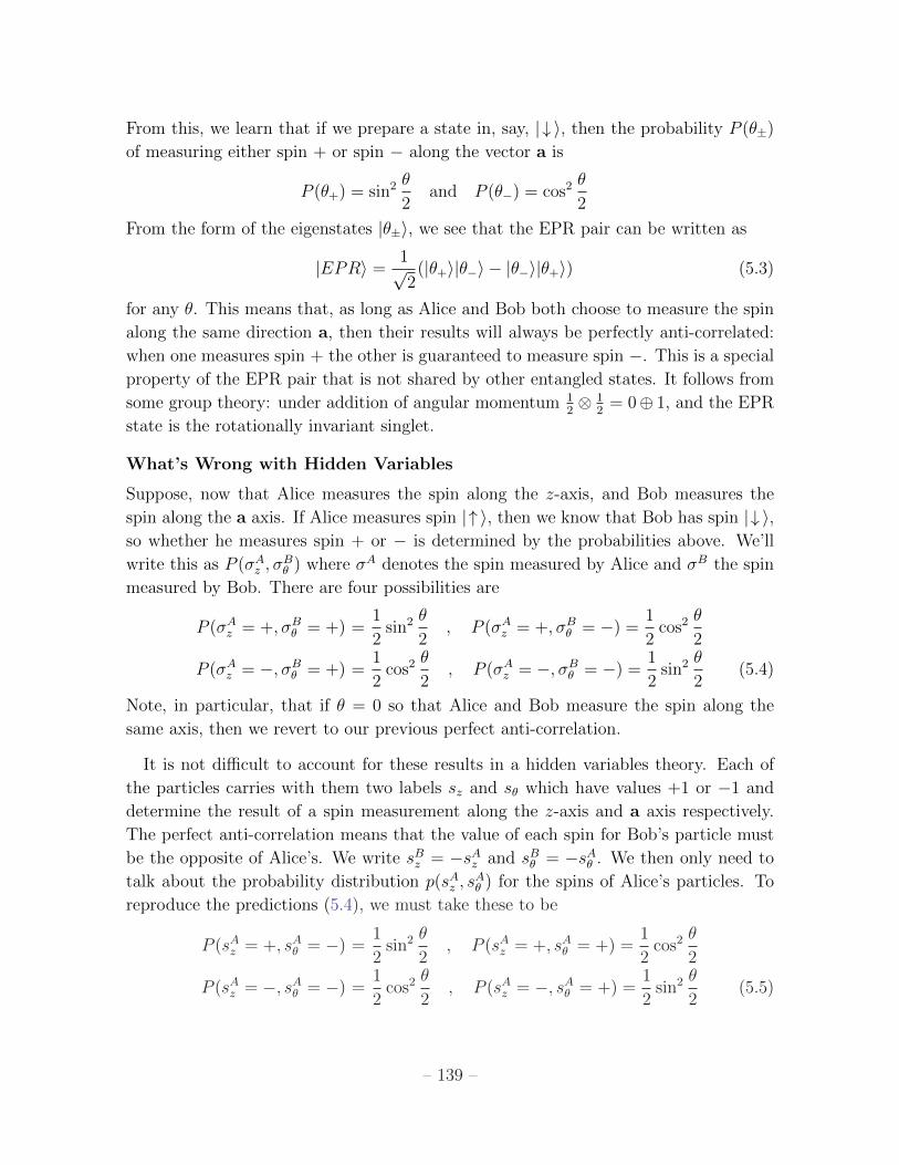
From this, we learn that if we prepare a state in, say, |# i, then the probability P (✓±)

of measuring either spin + or spin � along the vector a is

P (✓+) = sin2 ✓

2and P (✓�) = cos2

✓

2

From the form of the eigenstates |✓±i, we see that the EPR pair can be written as

|EPRi = 1p2(|✓+i|✓�i � |✓�i|✓+i) (5.3)

for any ✓. This means that, as long as Alice and Bob both choose to measure the spin

along the same direction a, then their results will always be perfectly anti-correlated:

when one measures spin + the other is guaranteed to measure spin �. This is a special

property of the EPR pair that is not shared by other entangled states. It follows from

some group theory: under addition of angular momentum 12 ⌦

12 = 0� 1, and the EPR

state is the rotationally invariant singlet.

What’s Wrong with Hidden Variables

Suppose, now that Alice measures the spin along the z-axis, and Bob measures the

spin along the a axis. If Alice measures spin |" i, then we know that Bob has spin |# i,so whether he measures spin + or � is determined by the probabilities above. We’ll

write this as P (�Az , �

B✓ ) where �

A denotes the spin measured by Alice and �B the spin

measured by Bob. There are four possibilities are

P (�Az = +, �B

✓ = +) =1

2sin2 ✓

2, P (�A

z = +, �B✓ = �) = 1

2cos2

✓

2

P (�Az = �, �B

✓ = +) =1

2cos2

✓

2, P (�A

z = �, �B✓ = �) = 1

2sin2 ✓

2(5.4)

Note, in particular, that if ✓ = 0 so that Alice and Bob measure the spin along the

same axis, then we revert to our previous perfect anti-correlation.

It is not di�cult to account for these results in a hidden variables theory. Each of

the particles carries with them two labels sz and s✓ which have values +1 or �1 and

determine the result of a spin measurement along the z-axis and a axis respectively.

The perfect anti-correlation means that the value of each spin for Bob’s particle must

be the opposite of Alice’s. We write sBz = �sAz and sB✓ = �sA✓ . We then only need to

talk about the probability distribution p(sAz , sA✓ ) for the spins of Alice’s particles. To

reproduce the predictions (5.4), we must take these to be

P (sAz = +, sA✓ = �) = 1

2sin2 ✓

2, P (sAz = +, sA✓ = +) =

1

2cos2

✓

2

P (sAz = �, sA✓ = �) = 1

2cos2

✓

2, P (sAz = �, sA✓ = +) =

1

2sin2 ✓

2(5.5)

– 139 –

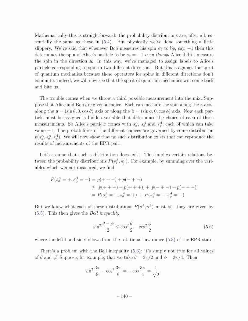
Mathematically this is straightforward: the probability distributions are, after all, es-

sentially the same as those in (5.4). But physically we’ve done something a little

slippery. We’ve said that whenever Bob measures his spin �✓ to be, say, +1 then this

determines the spin of Alice’s particle to be s✓ = �1 even though Alice didn’t measure

the spin in the direction a. In this way, we’ve managed to assign labels to Alice’s

particle corresponding to spin in two di↵erent directions. But this is against the spirit

of quantum mechanics because these operators for spins in di↵erent directions don’t

commute. Indeed, we will now see that the spirit of quantum mechanics will come back

and bite us.

The trouble comes when we throw a third possible measurement into the mix. Sup-

pose that Alice and Bob are given a choice. Each can measure the spin along the z-axis,

along the a = (sin ✓, 0, cos ✓) axis or along the b = (sin�, 0, cos�) axis. Now each par-

ticle must be assigned a hidden variable that determines the choice of each of these

measurements. So Alice’s particle comes with sAz , sA✓ and sA� , each of which can take

value ±1. The probabilities of the di↵erent choices are governed by some distribution

p(sAz , sA✓ , s

A� ). We will now show that no such distribution exists that can reproduce the

results of measurements of the EPR pair.

Let’s assume that such a distribution does exist. This implies certain relations be-

tween the probability distributions P (sAi , sAj ). For example, by summing over the vari-

ables which weren’t measured, we find

P (sA✓ = +, sA� = �) = p(+ +�) + p(�+�) [p(+ +�) + p(+ + +)] + [p(�+�) + p(���)]= P (sAz = +, sA✓ = +) + P (sAz = �, sA� = �)

But we know what each of these distributions P (sA, sA) must be: they are given by

(5.5). This then gives the Bell inequality

sin2 ✓ � �2 cos2

✓

2+ cos2

�

2(5.6)

where the left-hand side follows from the rotational invariance (5.3) of the EPR state.

There’s a problem with the Bell inequality (5.6): it’s simply not true for all values

of ✓ and �! Suppose, for example, that we take ✓ = 3⇡/2 and � = 3⇡/4. Then

sin2 3⇡

8� cos2

3⇡

8= � cos

3⇡

4=

1p2

– 140 –

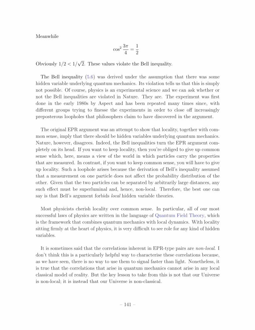
Meanwhile

cos23⇡

4=

1

2

Obviously 1/2 < 1/p2. These values violate the Bell inequality.

The Bell inequality (5.6) was derived under the assumption that there was some

hidden variable underlying quantum mechanics. Its violation tells us that this is simply

not possible. Of course, physics is an experimental science and we can ask whether or

not the Bell inequalities are violated in Nature. They are. The experiment was first

done in the early 1980s by Aspect and has been repeated many times since, with

di↵erent groups trying to finesse the experiments in order to close o↵ increasingly

preposterous loopholes that philosophers claim to have discovered in the argument.

The original EPR argument was an attempt to show that locality, together with com-

mon sense, imply that there should be hidden variables underlying quantum mechanics.

Nature, however, disagrees. Indeed, the Bell inequalities turn the EPR argument com-

pletely on its head. If you want to keep locality, then you’re obliged to give up common

sense which, here, means a view of the world in which particles carry the properties

that are measured. In contrast, if you want to keep common sense, you will have to give

up locality. Such a loophole arises because the derivation of Bell’s inequality assumed

that a measurement on one particle does not a↵ect the probability distribution of the

other. Given that the two particles can be separated by arbitrarily large distances, any

such e↵ect must be superluminal and, hence, non-local. Therefore, the best one can

say is that Bell’s argument forbids local hidden variable theories.

Most physicists cherish locality over common sense. In particular, all of our most

successful laws of physics are written in the language of Quantum Field Theory, which

is the framework that combines quantum mechanics with local dynamics. With locality

sitting firmly at the heart of physics, it is very di�cult to see role for any kind of hidden

variables.

It is sometimes said that the correlations inherent in EPR-type pairs are non-local. I

don’t think this is a particularly helpful way to characterise these correlations because,

as we have seen, there is no way to use them to signal faster than light. Nonetheless, it

is true that the correlations that arise in quantum mechanics cannot arise in any local

classical model of reality. But the key lesson to take from this is not that our Universe

is non-local; it is instead that our Universe is non-classical.

– 141 –

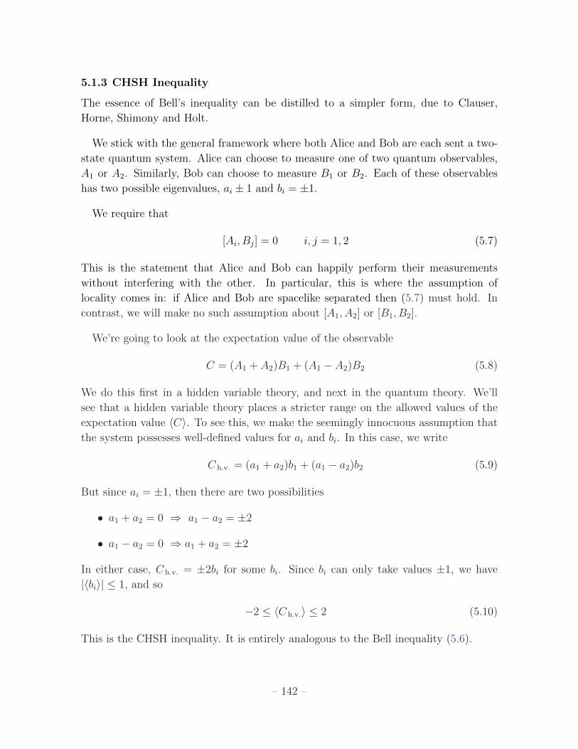
5.1.3 CHSH Inequality

The essence of Bell’s inequality can be distilled to a simpler form, due to Clauser,

Horne, Shimony and Holt.

We stick with the general framework where both Alice and Bob are each sent a two-

state quantum system. Alice can choose to measure one of two quantum observables,

A1 or A2. Similarly, Bob can choose to measure B1 or B2. Each of these observables

has two possible eigenvalues, ai ± 1 and bi = ±1.

We require that

[Ai, Bj] = 0 i, j = 1, 2 (5.7)

This is the statement that Alice and Bob can happily perform their measurements

without interfering with the other. In particular, this is where the assumption of

locality comes in: if Alice and Bob are spacelike separated then (5.7) must hold. In

contrast, we will make no such assumption about [A1, A2] or [B1, B2].

We’re going to look at the expectation value of the observable

C = (A1 + A2)B1 + (A1 � A2)B2 (5.8)

We do this first in a hidden variable theory, and next in the quantum theory. We’ll

see that a hidden variable theory places a stricter range on the allowed values of the

expectation value hCi. To see this, we make the seemingly innocuous assumption that

the system possesses well-defined values for ai and bi. In this case, we write

C h.v. = (a1 + a2)b1 + (a1 � a2)b2 (5.9)

But since ai = ±1, then there are two possibilities

• a1 + a2 = 0 ) a1 � a2 = ±2

• a1 � a2 = 0 ) a1 + a2 = ±2

In either case, C h.v. = ±2bi for some bi. Since bi can only take values ±1, we have

|hbii| 1, and so

�2 hC h.v.i 2 (5.10)

This is the CHSH inequality. It is entirely analogous to the Bell inequality (5.6).

– 142 –

What about in quantum theory? Now we don’t admit to a1 and a2 having simul-

taneous meaning, so we’re not allowed to write (5.9). Instead, we have to manipu-

late (5.8) as an operator equation. Because the eigenvalues are ±1, we must have

A21 = A2

2 = B21 = B2

2 = 1, the identity operator. After a little algebra, we find

C2 = 41� A1A2B1B2 + A2A1B1B2 + A1A2B2B1 � A2A1B2B1

= 41� [A1, A2][B1, B2]

Now |h[A1, A2]i| |hA1A2i| + |hA2A1i| 2, since each operator has eigenvalue ±1.

From this we learn that in the quantum theory,

hC2i 8

Since hC2i � hCi2, we find that the range of values in quantum mechanics to be

�2p2 hCi 2

p2

This is referred to as the Cirel’son bound. Clearly the range of values allowed by

quantum mechanics exceeds that allowed by hidden variables theories (5.10).

It remains for us to exhibit states and operators which violate the CHSH bound. For

this, we can return to our spin model. From (5.4), we know that

hEPR| �Az ⌦ �B

✓ |EPRi = sin2 ✓

2� cos2

✓

2= � cos ✓

This means that if we take the four operators A2, B1, A1 and B2 to be spin operators,

aligned in the (x, y) at successive angles of 45�. (i.e. A2 has ✓ = 0, B1 has ✓ = ⇡4 , A1

has ✓ = ⇡2 and B2 has ✓ = 3⇡

4 ) then

hA1B1i = hA1B1i = hA1B1i = �1p2

and hA2B2i = +1p2

and we see that

hCi = �2p2

saturating the Cirel’son bound.

5.1.4 Entanglement Between Three Particles

If we consider the case of three particles rather than two, then there is even sharper

contradiction between the predictions of quantum mechanics and those of hidden vari-

ables theories. As before, we’ll take each particle to carry one of two states, with a

basis given by spins |" i and |# i, measured in the z-direction.

– 143 –

Consider the entangled three-particle state

|GHZi = 1p2(|" i|" i|" i � |# i|# i|# i)

named after Greenberger, Horne and Zeilinger. These three particles are sent to our

three intrepid scientists, each waiting patiently in far-flung corners of the galaxy. Each

of these scientists makes one of two measurements: they either measure the spin in the

x-direction, or they measure the spin in the y-direction. Obviously, each experiment

gives them the result +1 or �1.

The state |GHZi will result in correlations between the di↵erent measurements.

Suppose, for example, that two of the scientists measure �x and the other measures �y.

It is simple to check that

�Ax ⌦ �B

x ⌦ �Cy |GHZi = �A

x ⌦ �By ⌦ �C

x |GHZi = �Ay ⌦ �B

x ⌦ �Cx |GHZi = +|GHZi

In other words, the product of the scientist’s three measurements always equals +1.

It’s tempting to follow the hidden variables paradigm and assign a spin sx and syto each of these three particles. Let’s suppose we do so. Then the result above means

that

sAx sBx s

Cy = sAx s

By s

Cx = sAy s

Bx s

Cx = +1 (5.11)

But from this knowledge we can make a simple prediction. If we multiply all of these

results together, we get

(sAx sBx s

Cx )

2 sAy sBy s

Cy = +1 ) sAy s

By s

Cy = +1 (5.12)

where the implication follows from the fact that the spin variables can only take val-

ues ±1. The hidden variables tell us that whenever the correlations (5.11) hold, the

correlation (5.12) must also hold.

Let’s now look at what quantum mechanics tells us. Rather happily, |GHZi happensto be an eigenstate of �A

y ⌦ �By ⌦ �C

y . But we have

�Ay ⌦ �B

y ⌦ �Cy |GHZi = �|GHZi

In other words, the product of these three measurements must give �1. This is in stark

contradiction to the hidden variables result (5.12). Once again we see that local hidden

variables are incapable of reproducing the results of quantum mechanics.

– 144 –

If Only We Hadn’t Made Counterfactual Arguments...

In both the Bell and GHZ arguments, the mistake in assigning hidden variables can be

traced to our use of counterfactuals. This is the idea that we can say what would have

happened had we made di↵erent choices.

Suppose, for example, that Alice chooses to measure �z to be +1 in an EPR state.

Then Bob can be absolutely certain that he will find �z to be �1 should he choose to

measure it. But even that certainty doesn’t give him the right to assign sBz = �1 unless

he actually goes ahead and measures it. This is because he may want to measure spin

along some other axis, �B✓ , and assuming that both properties exist will lead us to the

wrong conclusion as we’ve seen above. The punchline is that you don’t get to make

counterfactual arguments based on what would have happened: only arguments based

on what actually did happen.

5.1.5 The Kochen-Specker Theorem

The Kochen-Specker theorem provides yet another way to restrict putative hidden-

variables theories. Here is the statement:

Consider a set of N Hermitian operators Ai acting on H. Typically some of these

operators will commute with each other, while others will not. Any subset of operators

which mutually commute will be called compatible.

In an attempt to build a hidden variables theory, all observables Ai are assigned a

value ai 2 R. We will require that whenever A, B and C 2 {Ai} are compatible then

the following properties should hold

• If C = A+B then c = a+ b.

• If C = AB then c = ab.

These seem like sensible requirements. Indeed, in quantum mechanics we know that if

[A,B] = 0 then the expectation values obey the relations above and, moreover, there

are states where we can assign definite values to A, B and therefore to A + B and to

AB. We will not impose any such requirements if [A,B] 6= 0.

As innocuous as these requirements may seem, the Kochen-Specker theorem states

that in Hilbert spaces H with dimension dim(H) � 3, there are sets of operators {Ai}for which it is not possible to assign values ai with these properties. Note that this

isn’t a statement about a specific state in the Hilbert space; it’s a stronger statement

that there is no consistent values that can possibly be assigned to operators.

– 145 –

The issue is that a given operator, say A, can be compatible with many di↵erent

operators. So, for example, it may appear in the compatible set (A,B,C) and also in

(A,D,E) and should take the same value a in both. Meanwhile, B may appear in a

di↵erent compatible set and so on. The proofs of the Kochen-Specker theorem involve

exhibiting a bunch of operators which cannot be consistently assigned values.

The original proof of the Kocken-Specker theorem is notoriously fiddly, involving a

set of N = 117 di↵erent projection operators in a dim(H) = 3 dimensional Hilbert

space4. Simpler versions of the proof with dim(H) = 3 now exist, although we won’t

present them here.

There is, however, a particularly straightforward proof that involves N = 18 opera-

tors in a dim(H) = 4 dimensional Hilbert space. We start by considering the following

18 vectors i 2 C4,

1 = (0, 0, 0, 1) , 2 = (0, 0, 1, 0) , 3 = (1, 1, 0, 0) , 4 = (1,�1, 0, 0) 5 = (0, 1, 0, 0) , 6 = (1, 0, 1, 0) , 7 = (1, 0,�1, 0) , 8 = (1,�1, 1,�1)

9 = (1,�1,�1, 1) , 10 = (0, 0, 1, 1) , 11 = (1, 1, 1, 1) , 12 = (0, 1, 0,�1) 13 = (1, 0, 0, 1) , 14 = (1, 0, 0,�1) , 15 = (0, 1,�1, 0) , 16 = (1, 1,�1, 1)

17 = (1, 1, 1,�1) , 18 = (�1, 1, 1, 1)

From each of these, we can build a projection operator

Pi =| iih i|h i| ii

Since the projector operators can only take eigenvalues 0 or 1, we want to assign a

value pi = 0 or pi = 1 to each projection operator Pi.

Of course, most of these projection operators do not commute with each other.

However, there are subsets of four such operators which mutually commute and sum

to give the identity operator. For example,

P1 + P2 + P3 + P4 = 14

In this case, the requirements of the Kocken-Specker theorem tell us that one of these

operators must have value p = 1 and the other three must have value p = 0.

4More details can be found at https://plato.stanford.edu/entries/kochen-specker/.

– 146 –

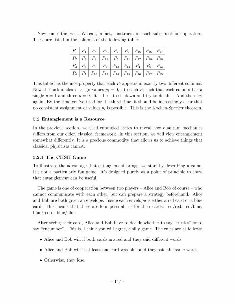
Now comes the twist. We can, in fact, construct nine such subsets of four operators.

These are listed in the columns of the following table:

P1 P1 P8 P8 P2 P9 P16 P16 P17

P2 P5 P9 P11 P5 P11 P17 P18 P18

P3 P6 P3 P7 P13 P14 P4 P6 P13

P4 P7 P10 P12 P14 P15 P10 P12 P15

This table has the nice property that each Pi appears in exactly two di↵erent columns.

Now the task is clear: assign values pi = 0, 1 to each Pi such that each column has a

single p = 1 and three p = 0. It is best to sit down and try to do this. And then try

again. By the time you’ve tried for the third time, it should be increasingly clear that

no consistent assignment of values pi is possible. This is the Kochen-Specker theorem.

5.2 Entanglement is a Resource

In the previous section, we used entangled states to reveal how quantum mechanics

di↵ers from our older, classical framework. In this section, we will view entanglement

somewhat di↵erently. It is a precious commodity that allows us to achieve things that

classical physicists cannot.

5.2.1 The CHSH Game

To illustrate the advantage that entanglement brings, we start by describing a game.

It’s not a particularly fun game. It’s designed purely as a point of principle to show

that entanglement can be useful.

The game is one of cooperation between two players – Alice and Bob of course – who

cannot communicate with each other, but can prepare a strategy beforehand. Alice

and Bob are both given an envelope. Inside each envelope is either a red card or a blue

card. This means that there are four possibilities for their cards: red/red, red/blue,

blue/red or blue/blue.

After seeing their card, Alice and Bob have to decide whether to say “turtles” or to

say “cucumber”. This is, I think you will agree, a silly game. The rules are as follows:

• Alice and Bob win if both cards are red and they said di↵erent words.

• Alice and Bob win if at least one card was blue and they said the same word.

• Otherwise, they lose.

– 147 –

What’s their best strategy? First suppose that Alice and Bob are classical losers and

have no help from quantum mechanics. It’s not hard to convince yourself that their

best strategy is just to say “cucumber” every time, regardless of the colour of their

card. They only lose if both cards turn out to be red. Otherwise they win. This means

that they win 75% of the time.

Suppose, however, that Alice and Bob have spent many decades developing coherent

qubits. This pioneering technology resulted in them being kidnapped by a rival govern-

ment who then, for reasons hard to fathom, subjected them to this stupid game. Can

their discoveries help them get out of a bind? Thankfully, the answer is yes. Although,

arguably, not so much that it’s worth all the trouble.

To do better, Alice and Bob must share a number of EPR pairs, one for each time

that the game is played. Here is their gameplan. Whenever Alice’s card is blue, she

measures A1; whenever it is red she measures A2. Whenever these measurements give

+1 she says “turtles”; whenever it is �1 she says “cucumber”. Bob does something

similar: B1 when blue, B2 when red; “turtles” when +1, “cucumber” when �1.

Suppose that both cards are blue. Then they win if A1 and B1 give the same result

and lose otherwise. In other words, they win if the measurement gives A1B1 = +1 and

lose when A1B1 = �1. This means

P (win)� P (lose) = hA1B1i

In contrast, if both cards are red then they lose if A2 and B2 give the same measurement

and win otherwise, so that

P (win)� P (lose) = �hA2B2i

Since each combination of cards arises with probability p = 14 , the total probability is

P (win)� P (lose) =1

4hA1B1 + A1B2 + A2B1 � A2B2i

But we’ve seen this before: it’s precisely the combination of operators (5.8) that arose

in the CHSH proof of the Bell inequality. We can immediately import our answer from

there to learn that

P (win)� P (lose) 1p2

We saw previously that we can find operators which saturate this inequality. Since

P (win) + P (lose) = 1, there’s a choice of measurements Ai and Bi — essentially spin

– 148 –

measurements which di↵er by 45� — which ensures a win rate of

P (win) =1

2

✓1p2+ 1

◆⇡ 0.854

This beats our best classical strategy of 75%.

Having the ability to win at this particular game is unlikely to change the world.

Obviously the game was cooked up by starting from the CHSH inequality and working

backwards in an attempt to translate Bell’s inequality into something approximating

a game. But it does reveal an important point: the correlations in entangled states

can be used to do things that wouldn’t otherwise be possible. If we can harness this

ability to perform tasks that we actually care about, then we might genuinely be able

to change the world. This is the subject of quantum information. Here we give a couple

of simple examples that move in this direction.

5.2.2 Dense Coding

For our first application, Alice wants to send Bob some classical information, which

means she wants to tell him “yes” or “no” to a series of questions. This is encoded in

a classical bit as values 0 and 1.

However, Alice is fancy. She has qubits at her disposal and can send these to Bob.

We’d like to know if she can use this quantum technology to aid in sending her classical

information.

First note that Alice doesn’t lose anything by sending qubits rather than classical

bits. (Apart, of course, from the hundreds of millions of dollars in R&D that it took to

get them in the first place.) She could always encode the classical value 0 as |" i and1 as | # i and, provided Bob is told in advance to measure �z, the qubit contains the

same information as a classical bit. But this does seem like a waste of resources.

Is it possible to do better and transmit more than one classical bit in a single qubit?

The answer is no: a single qubit carries the same amount of information as a classical

bit. However, this changes if Alice’s qubit is actually part of an entangled pair that

she shares with Bob. In this case, she can encode two classical bits of information in a

single qubit. This is known as dense coding.

To achieve this feat, Alice first performs an operation on her spin. We’ll introduce

some new notation for this state that will become useful in the following section: we

call the EPR pair

|EPRi = |��i = 1p2(|" i|# i � |# i|" i)

– 149 –

Alice then has four options:

• She does nothing. Obviously, the entangled pair remains in the state |��i.

• Alice acts with �x. This changes the state to �|��i where

|��i = 1p2(|" i|" i � |# i|# i)

• Alice acts with �y. This changes the state to �i|�+i where

|�+i = 1p2(|" i|" i+ |# i|# i)

• Alice acts with �z. This changes the state to |�+i.

|�+i = 1p2(|" i|# i+ |# i|" i)

The upshot of this procedure is that the entangled pair sits in one of four di↵erent

states

|�±i = 1p2(|" i|" i± |# i|# i) or |�±i = 1p

2(|" i|# i± |# i|" i) (5.13)

Alice now sends her qubit to Bob, so Bob has access to the whole entangled state.

Since the four di↵erent states are orthogonal, it must be possible to distinguish them

by performing some measurements. Indeed, the measurements Bob needs to make are

�x ⌦ �x and �z ⌦ �z

These two operators commute. This means that, while we don’t get to know the values

of both sx and sz of, say, the first spin, it does make sense to talk about the products

of the spins of the two qubits in both directions. It’s simple to check that the four

possible states above are eigenstates of these two operators

�x ⌦ �x|�±i = ±|�±i and �x ⌦ �x|�±i = ±|�±i (5.14)

�z ⌦ �z|�±i = +|�±i and �z ⌦ �z|�±i = �|�±i

So, for example, if Bob measures �x ⌦ �x = +1 and �z ⌦ �z = �1, then he knows that

he’s in possession of state |�+i. Bob then knows which of the four operations Alice

performed. In this way she has communicated two classical bits of information through

the exchange of a single qubit.

– 150 –

Admittedly, two qubits were needed for this to fly: one which was exchanged and

one which was in Bob’s possession all along. In fact, in Section 5.3.2, we’ll show that

entanglement between spins can only be created if the two spins were brought together

at some point in the past. So, from this point of view, Alice actually exchanged two

qubits with Bob, the first long ago when they shared the EPR pair, and the second

when the message was sent. Nonetheless, there’s still something surprising about dense

coding. The original EPR pair contained no hint of the message that Alice wanted

to send; indeed, it could have been created long before she knew what that message

was. Nor was there any information in the single qubit that Alice sent to Bob. Anyone

intercepting it along the way would be no wiser. It’s only when this qubit is brought

together with Bob’s that the information becomes accessible.

5.2.3 Quantum Teleportation

Our next application has a sexy sounding name: quantum teleportation. To put it in

context, we first need a result that tells us what we cannot do in quantum mechanics.

The No Cloning Theorem

The no cloning theorem says that it is impossible to copy a state in quantum mechanics.

Here’s the game. Someone gives you a state | i, but doesn’t tell you what that state

is. Now, you can determine some property of the state but any measurement that you

make will alter the state. This means that you can’t then go back and ask di↵erent

questions about the initial state.

Our inability to know everything about a state is one of the key tenets of quantum

mechanics. But there’s an obvious way around it. Suppose that we could just copy the

initial state many times. Then we could ask di↵erent questions on each of the replicas

and, in this way, build up a fuller picture of the original state. The no cloning theorem

forbids this.

To prove the theorem, we really only need to set up the question. We start with a

state | i 2 HA. Suppose that we prepare a separate system in a blank state |0i 2 HB.

To create a copy of the initial state, we would like to evolve the system so that

|In( )i = | i ⌦ |0i �! |Out( )i = | i ⌦ | i

But this can’t happen through any Hamiltonian evolution because it is not a unitary

operation. To see this, consider two di↵erent states | 1i and | 2i. We have

hIn( 1)|In( 2)i = h 1| 2i while hOut( 1)|Out( 2)i = h 1| 2i2

– 151 –

We might try to wriggle out of this conclusion by allowing for some other stu↵ in the

Hilbert space which can change in any way it likes. This means that we now have three

Hilbert spaces and are looking an evolution of the form

| i ⌦ |0i ⌦ |↵(0)i �! | i ⌦ | i ⌦ |↵( )i

By linearity, if such an evolution exists it must map

(|�i+ | i)⌦ |0i ⌦ |↵(0)i �! |�i ⌦ |�i ⌦ |↵(�)i+ | i ⌦ | i ⌦ |↵( )i (5.15)

But this isn’t what we wanted! The map is supposed to take

(|�i+ | i)⌦ |0i ⌦ |↵(0)i �! (|�i+ | i)⌦ (|�i+ | i)⌦ |↵( + �)i= (|�i|�i+ | i|�i+ |�i| i+ | i| i)⌦ |↵( + �)i

where, in the last line, we dropped the ⌦ between the first two Hilbert spaces. The

state that we get (5.15) is not the state that we want. This concludes our proof of the

no cloning theorem.

Back to Teleportation

With the no cloning theorem as background, we can now turn to the idea of quantum

teleportation. Alice is given a qubit in state | i. The challenge is to communicate this

state to Bob.

There are two limitations. First, Alice doesn’t get to simply put the qubit in the mail.

That’s no longer the game. Instead, she must describe the qubit to Bob using classical

information: i.e. bits, not qubits. Note that we’re now playing by di↵erent rules from

the previous section. In “dense coding” we wanted to send classical information using

qubits. Here we want to send quantum information using classical bits.

Now this sounds like teleportation must be impossible. As we’ve seen, Alice has no

way of figuring out what state | i she has. If she doesn’t know the state, how on earth

is she going to communicate it to Bob? Well, magically, there is way. For this to work,

Alice and Bob must also share an EPR pair. We will see that they can sacrifice the

entanglement in this EPR pair to allow Bob to reproduce the state | i.

First, Alice. She has two qubits: the one we want to transfer, | i, together with the

her half of the pair |EPRi. She makes the following measurements:

�x ⌦ �x and �z ⌦ �z

where, in each case, the first operator acts on | i and the second on her half of |EPRi.

– 152 –

As we saw in the previous section, these are commuting operators, each with eigen-

values ±1. This means that there are four di↵erent outcomes to Alice’s experiment

and the state will be projected onto the eigenstates |�±i or |�±i defined in (5.13). The

di↵erent possible outcomes of the measurement were given in (5.14).

Let’s see what becomes of the full state after Alice’s measurements. We write the

unknown qubit | i as

| i = ↵|" i+ �|# i (5.16)

with |↵|2 + |�|2 = 1. Then the full state of three qubits – two owned by Alice and one

by Bob – is

| i ⌦ |EPRi = 1p2

⇣↵|" i|" i|# i � ↵|" i|# i|" i+ �|# i|" i|# i � �|# i|# i|" i

⌘

=1

2

⇣↵(|�+i+ |��i)|# i � ↵(|�+i+ |��i)|" i

+�(|�+i � |��i)|# i � �(|�+i � |��i)|" i⌘

=1

2

⇣|�+i(��|" i+ ↵|# i) + |��i(�|" i+ ↵|# i)

+|�+i(�↵|" i+ �|# i)� |��i(↵|" i+ �|# i)⌘

When Alice makes her measurement, the wavefunction collapses onto one of the four

eigenstates |�±i or |�±i. But we see that Bob’s state — the final one in the wavefunction

above — has taken the form of a linear superposition of | " i and | # i, with the same

coe�cients ↵ and � that characterised the initial state | i in (5.16). Now, in most of

these cases, Bob’s state isn’t exactly the same as | i, but that’s easily fixed if Bob acts

with a unitary operator. All Alice has to do is tell Bob which of the four states she

measured and this will be su�cient for Bob to know how he has to act. Let’s look at

each in turn.

• If Alice measures |�+i then Bob should operate on his qubit with �y to get

�y(��|" i+ ↵|# i) = i�|# i+ i↵|" i = i| i

which, up to a known phase, is Alice’s initial state.

• If Alice measures |��i then Bob should operate on his qubit with �x,

�x(�|" i+ ↵|# i) = �|# i+ ↵|" i = | i

– 153 –

• If Alice measures |�+i then Bob should operate on his qubit with �z,

�x(�|" i+ ↵|# i) = �|# i+ ↵|" i = | i

• If Alice measures |�+i, Bob can put his feet up and do nothing. He already has

�| i sitting in front of him.

We see that if Alice sends Bob two bits of information — enough to specify which of

the four states she measured — then Bob can ensure that he gets state | i. Note thatthis transfer occurred with neither Alice nor Bob knowing what the state | i actuallyis. But Bob can be sure that he has it.

5.2.4 Quantum Key Distribution

If you want to share a secret, it’s best to have a code. Here is an example of an

unbreakable code. Alice and Bob want to send a message consisting of n classical bits,

a string of 0’s and 1’s. To do so securely, they must share, in advance, a private key.

This is a string of classical bits that is the same length as the message. Alice simply

adds the key to the message bitwise (0 + 0 = 1 + 1 = 0 and 0 + 1 = 1 + 0 = 1) before

sending it to Bob who, upon receiving it, subtracts the key to reveal the message. Any

third party eavesdropper – traditionally called Eve – who intercepts the transmission

is none the wiser.

The weakness of this approach is that, to be totally secure, Alice and Bob, should

use a di↵erent key for each message that they want to send. If they fail to do this then

Eve can use some knowledge about the underlying message (e.g. it’s actually written in

German and contains information about U-boat movements in the Atlantic) to detect

correlations in the transmissions and, ultimately, crack the code. This means that Alice

and Bob must have a large supply of private keys and be sure that Eve does not have

access to them. This is where quantum mechanics can be useful.

BB84

BB84 is a quantum protocol for generating a secure private key. It’s named after its

inventors, Bennett and Brassard, who suggested this approach in 1984.

The idea is remarkably simple. Alice takes a series of qubits. For each, she chooses

to measure the spin either in the z-direction, or in the x-direction. This leaves her with

a qubit in one of four possible states: | " i, | # i, |!i or | i. Alice then sends this

qubit to Bob. He has no idea which measurement Alice made, so he makes a random

decision to measure the spin in either the z-direction or the x-direction. About half

the time he will make the same measurement as Alice, the other half he will make a

di↵erent measurement.

– 154 –

Having performed these experiments, Alice and Bob then announce publicly which

spin measurements they made. Whenever they measured the spin in di↵erent direc-

tions, they simply discard their results. Whenever they measured the spin in the same

direction, the measurements must agree. This becomes their private key.

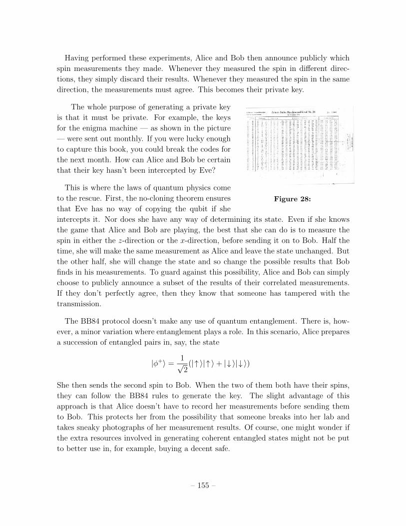
The whole purpose of generating a private key

Figure 28:

is that it must be private. For example, the keys

for the enigma machine — as shown in the picture

— were sent out monthly. If you were lucky enough

to capture this book, you could break the codes for

the next month. How can Alice and Bob be certain

that their key hasn’t been intercepted by Eve?

This is where the laws of quantum physics come

to the rescue. First, the no-cloning theorem ensures

that Eve has no way of copying the qubit if she

intercepts it. Nor does she have any way of determining its state. Even if she knows

the game that Alice and Bob are playing, the best that she can do is to measure the

spin in either the z-direction or the x-direction, before sending it on to Bob. Half the

time, she will make the same measurement as Alice and leave the state unchanged. But

the other half, she will change the state and so change the possible results that Bob

finds in his measurements. To guard against this possibility, Alice and Bob can simply

choose to publicly announce a subset of the results of their correlated measurements.

If they don’t perfectly agree, then they know that someone has tampered with the

transmission.

The BB84 protocol doesn’t make any use of quantum entanglement. There is, how-

ever, a minor variation where entanglement plays a role. In this scenario, Alice prepares

a succession of entangled pairs in, say, the state

|�+i = 1p2(|" i|" i+ |# i|# i)

She then sends the second spin to Bob. When the two of them both have their spins,

they can follow the BB84 rules to generate the key. The slight advantage of this

approach is that Alice doesn’t have to record her measurements before sending them

to Bob. This protects her from the possibility that someone breaks into her lab and

takes sneaky photographs of her measurement results. Of course, one might wonder if

the extra resources involved in generating coherent entangled states might not be put

to better use in, for example, buying a decent safe.

– 155 –

The moral behind quantum key distribution is clear: quantum information is more

secure than classical information because no one, whether friend or enemy, can be sure

what quantum state they’ve been given.

5.3 Density Matrices

In Section 5.1, we’ve made a big deal out the fact that quantum correlations cannot

be captured by classical probability distributions. In the classical world, uncertainty

is due to ignorance: the more you know, the better your predictions. In the quantum

world, the uncertainty is inherent and can’t be eliminated by gaining more knowledge.

There are situations in the quantum world where we have to deal with both kinds

of uncertainties. There are at least two contexts in which this arises. One possibility

is ignorance: we simply don’t know for sure what quantum state our system lies in.

Another possibility is that we have many quantum states — an ensemble — and they

don’t all lie in the same state, but rather in a mixture of di↵erent states. In either

context, we use the same mathematical formalism.

Suppose that we don’t know which of the states | ii describes our system. These

states need not be orthogonal – just di↵erent. To parameterise our ignorance, we assign

classical probabilities pi to each of these states. The expectation value of any operator

A is given by

hAi =X

i

pih i|A| ii (5.17)

This expression includes both classical uncertainty (in the pi) and quantum uncertainty

(in the h i|A| ii).

Such a state is described by an operator known as the density matrix.

⇢ =X

i

pi| iih i| (5.18)

Clearly, this is a sum of projections onto the spaces spanned by | ii, weighted with

the probabilities pi. The expectation value (5.17) of any operator can now be written

simply as

hAi = Tr(⇢A)

where the trace is over all states in the Hilbert space.

– 156 –

Pure States vs Mixed States

Previously, we thought that the state of a quantum system is described by a normalised

vector in the Hilbert space. The density matrix is a generalisation of this idea to

incorporate classical probabilities. If we’re back in the previous situation, where we

know for sure that the system is described by a specific state | i, then the density

matrix is simply the projection operator

⇢ = | ih |

In this case, we say that we have a pure state. If the density matrix cannot be written

in this form then we say that we have a mixed state. Note that a pure state has the

property that

⇢2 = ⇢

Regardless of whether a state is pure or mixed, the density matrix encodes all our

information about the state and allows us to compute the expected outcome of any

measurement. Note that the density matrix does not contain information about the

phases of the states | ii since these have no bearing on any physical measurement.

Properties of the Density Matrix

The density matrix (5.18) has the following properties

• It is self-adjoint: ⇢ = ⇢†

• It has unit trace: Tr⇢ = 1. This property is equivalent to the normalisation of a

probability distribution, so thatP

i pi = 1.

• It is positive: h�|⇢|�i � 0 for all |�i 2 H. This property, which strictly speaking

should be called “non-negative”, is equivalent to the requirement that pi � 0. As

shorthand, we sometimes write the positivity requirement simply as ⇢ � 0.

Furthermore, any operator ⇢ which satisfies these three properties can be viewed as a

density matrix for a quantum system. To see this, we can look at the eigenvectors of

⇢, given by

⇢|�ni = pn|�ni

where, here, pn is simply the corresponding eigenvalue. Because ⇢ = ⇢†, we know that

pn 2 R. The second two properties above then tell us thatP

n pn = 1 and pn � 0.

– 157 –

This is all we need to interpret pn as a probability distribution. We can then write ⇢

as

⇢ =X

n

pn|�nih�n| (5.19)

This way of writing the density matrix is a special case of (5.18). It’s special because

the |�ni are eigenvectors of a Hermitian matrix and, hence, orthogonal. In contrast, the

vector | ii in (5.18) are not necessarily orthonormal. However, although the expression

(5.19) is special, there’s nothing special about ⇢ itself: any density matrix can be written

in this form. We’ll come back to this idea below when we discuss specific examples.

An Example: Statistical Mechanics

There are many places in physics where it pays to think of probability distributions

over ensembles of states. One prominent example is what happens for systems at finite

temperature T . This is the subject of Statistical Mechanics.

Recall that the Boltzmann distribution tells us that the probability pn that we sit in

an energy eigenstate |ni is given by

pn =e��En

Zwhere � =

1

kBTand Z =

X

n

e��En

where kB is the Boltzmann constant. It is straightforward to construct an density

matrix corresponding to this ensemble. It is given by

⇢ =e��H

Z(5.20)

where H is the Hamiltonian. Similarly, the partition function is given by

Z = Tr e��H

It is then straightforward to reformulate much of statistical mechanics in this language.

For example, the average energy of a system is hEi = Tr(⇢H).

In these lectures, we won’t necessarily be interested in the kind of macroscopic sys-

tems that arise in statistical physics. Instead, we’ll build some rather di↵erent intuition

for the meaning of the density matrix.

– 158 –

Time Evolution

Recall that in the Schrodinger picture, any state evolves as

| (t)i = U(t)| (0)i with U(t) = e�iHt/~

From this we learn that the density matrix evolves as

⇢(t) = U(t)⇢(0)U †(t)

Di↵erentiating with respect to t gives us a di↵erential equation governing time evolu-

tion,

@⇢

@t= � i

~ [H, ⇢] (5.21)

This is the Liouville equation. Or, more accurately, it is the quantum version of the

Liouville equation which we met in the Classical Dynamics lectures where it governs

the evolution of probability distributions on phase space.

Note that any density operator which depends only on the Hamiltonian H is inde-

pendent of time. The Boltzmann distribution (5.20) is the prime example.

5.3.1 The Bloch Sphere

As an example, let’s return to our favourite two-state system. If we measure spin along

the z-axis, then the two eigenstates are |" i and |# i.

Suppose that we know for sure that we’re in state |" i. Then, obviously,

⇢ = |" ih"|

If however, there’s probability p = 12 that we’re in state | " i and, correspondingly,

probability 1� p = 12 that we’re in state |# i, then

⇢ =1

2|" ih"|+ 1

2|# ih#| = 1

21 (5.22)

This is the state of maximum ignorance, something we will quantify below in Section

5.3.3. In particular, the average value for the spin along any axis always vanishes:

h�i = Tr(⇢�) = 0.

Let’s now consider other spin states. Consider the spin measured along the x-axis.

Suppose that there’s probability p = 12 that we’re in state |!i and probability 1�p = 1

2

that we’re in state | i, then

⇢ =1

2

h|!ih!|+ | ih |

i=

1

21 (5.23)

Once again, we find a state of maximum ignorance. This highlights an important fact:

given a density matrix ⇢, there is no unique way to decompose in the form (5.18).

– 159 –

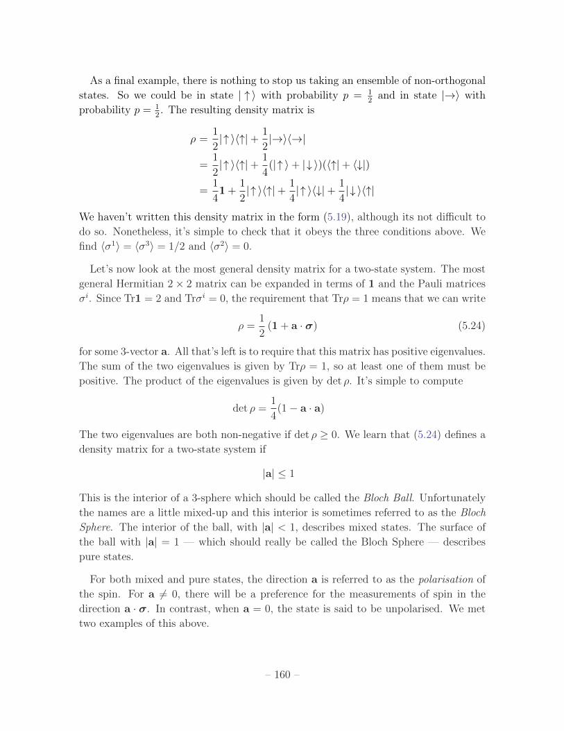
As a final example, there is nothing to stop us taking an ensemble of non-orthogonal

states. So we could be in state | " i with probability p = 12 and in state |!i with

probability p = 12 . The resulting density matrix is

⇢ =1

2|" ih"|+ 1

2|!ih!|

=1

2|" ih"|+ 1

4(|" i+ |# i)(h"|+ h#|)

=1

41+

1

2|" ih"|+ 1

4|" ih#|+ 1

4|# ih"|

We haven’t written this density matrix in the form (5.19), although its not di�cult to

do so. Nonetheless, it’s simple to check that it obeys the three conditions above. We

find h�1i = h�3i = 1/2 and h�2i = 0.

Let’s now look at the most general density matrix for a two-state system. The most

general Hermitian 2⇥ 2 matrix can be expanded in terms of 1 and the Pauli matrices

�i. Since Tr1 = 2 and Tr�i = 0, the requirement that Tr⇢ = 1 means that we can write

⇢ =1

2(1+ a · �) (5.24)

for some 3-vector a. All that’s left is to require that this matrix has positive eigenvalues.

The sum of the two eigenvalues is given by Tr⇢ = 1, so at least one of them must be

positive. The product of the eigenvalues is given by det ⇢. It’s simple to compute

det ⇢ =1

4(1� a · a)

The two eigenvalues are both non-negative if det ⇢ � 0. We learn that (5.24) defines a

density matrix for a two-state system if

|a| 1

This is the interior of a 3-sphere which should be called the Bloch Ball. Unfortunately

the names are a little mixed-up and this interior is sometimes referred to as the Bloch

Sphere. The interior of the ball, with |a| < 1, describes mixed states. The surface of

the ball with |a| = 1 — which should really be called the Bloch Sphere — describes

pure states.

For both mixed and pure states, the direction a is referred to as the polarisation of

the spin. For a 6= 0, there will be a preference for the measurements of spin in the

direction a · �. In contrast, when a = 0, the state is said to be unpolarised. We met

two examples of this above.

– 160 –

The Ambiguity of Preparation

The are typically many di↵erent interpretations of a density matrix. We’ve seen an

example above, where two di↵erent probability distributions over states (5.22) and

(5.23) both give rise to the same density matrix. It’s sometimes said that these density

matrices are prepared di↵erently, but describe the same state.

More generally, suppose that the system is described by density matrix ⇢1 with some

probability � and density matrix ⇢2 with some probability (1 � �). The expectation

value of any operator is determined by the density matrix

⇢(�) = �⇢1 + (1� �)⇢2

Indeed, nearly all density operators can be expressed as the sum of other density

operators in an infinite number of di↵erent ways.

There is an exception to this. If the density matrix ⇢ actually describes a pure state

then it cannot be expressed as the sum of two other states.

5.3.2 Entanglement Revisited

The density matrix has a close connection to the ideas of entanglement that we met in

earlier sections. Suppose that our Hilbert space decomposes into two subspaces,

H = HA ⌦HB

This is sometimes referred to as a bipartite decomposition of the Hilbert space. It really

means that HA and HB describe two di↵erent physical systems. In what follows, it will

be useful to think of these systems as far separated, so that they don’t interact with

each other. Nonetheless, as we’ve seen in Section 5.1, quantum states can be entangled

between these two systems, giving rise to correlations between measurements.

Let’s consider things from Alice’s perspective. She only has access to the system

described by HA. This means that she gets to perform measurements associated to

operators of the form

O = A⌦ 1

If the state of the full system is described by the density matrix ⇢AB, then measurements

Alice makes will have expectation value

hAi = TrHATrHB

⇣(A⌦ 1)⇢AB

⌘⌘ TrHA(A ⇢A)

– 161 –

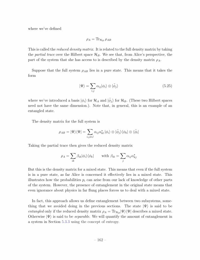
where we’ve defined

⇢A = TrHB ⇢AB

This is called the reduced density matrix. It is related to the full density matrix by taking

the partial trace over the Hilbert space HB. We see that, from Alice’s perspective, the

part of the system that she has access to is described by the density matrix ⇢A.

Suppose that the full system ⇢AB lies in a pure state. This means that it takes the

form

| i =X

i,j

↵ij|�ii ⌦ |�ji (5.25)

where we’ve introduced a basis |�ii for HA and |�ji for HB. (These two Hilbert spaces

need not have the same dimension.). Note that, in general, this is an example of an

entangled state.

The density matrix for the full system is

⇢AB = | ih | =X

i,j,k,l

↵ij↵?kl |�ii ⌦ |�jih�k|⌦ h�l|

Taking the partial trace then gives the reduced density matrix

⇢A =X

ik

�ik|�iih�k| with �ik =X

j

↵ij↵?kj

But this is the density matrix for a mixed state. This means that even if the full system

is in a pure state, as far Alice is concerned it e↵ectively lies in a mixed state. This

illustrates how the probabilities pi can arise from our lack of knowledge of other parts

of the system. However, the presence of entanglement in the original state means that

even ignorance about physics in far flung places forces us to deal with a mixed state.

In fact, this approach allows us define entanglement between two subsystems, some-

thing that we avoided doing in the previous sections. The state | i is said to be

entangled only if the reduced density matrix ⇢A = TrHB | ih | describes a mixed state.

Otherwise | i is said to be separable. We will quantify the amount of entanglement in

a system in Section 5.3.3 using the concept of entropy.

– 162 –

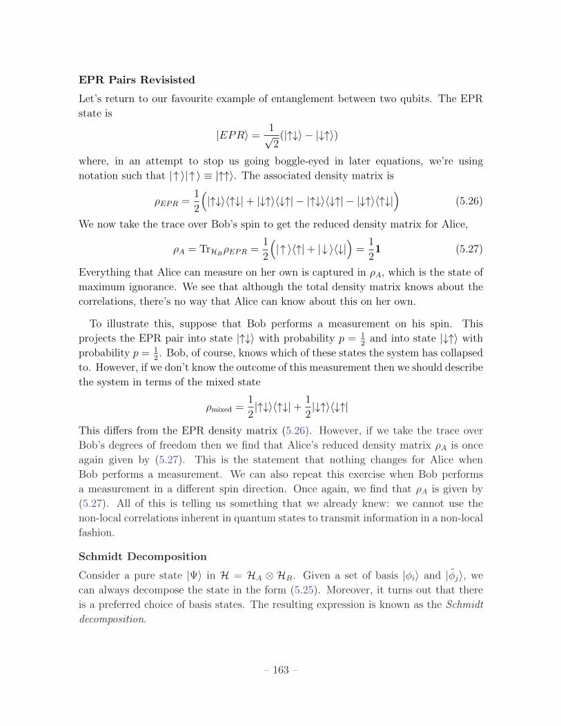
EPR Pairs Revisisted

Let’s return to our favourite example of entanglement between two qubits. The EPR

state is

|EPRi = 1p2(|"#i � |#"i)

where, in an attempt to stop us going boggle-eyed in later equations, we’re using

notation such that |" i|" i ⌘ |""i. The associated density matrix is

⇢EPR =1

2

⇣|"#ih"#|+ |#"ih#"|� |"#ih#"|� |#"ih"#|

⌘(5.26)

We now take the trace over Bob’s spin to get the reduced density matrix for Alice,

⇢A = TrHB⇢EPR =1

2

⇣|" ih"|+ |# ih#|

⌘=

1

21 (5.27)

Everything that Alice can measure on her own is captured in ⇢A, which is the state of

maximum ignorance. We see that although the total density matrix knows about the

correlations, there’s no way that Alice can know about this on her own.

To illustrate this, suppose that Bob performs a measurement on his spin. This

projects the EPR pair into state |"#i with probability p = 12 and into state |#"i with

probability p = 12 . Bob, of course, knows which of these states the system has collapsed

to. However, if we don’t know the outcome of this measurement then we should describe

the system in terms of the mixed state

⇢mixed =1

2|"#ih"#|+ 1

2|#"ih#"|

This di↵ers from the EPR density matrix (5.26). However, if we take the trace over

Bob’s degrees of freedom then we find that Alice’s reduced density matrix ⇢A is once

again given by (5.27). This is the statement that nothing changes for Alice when

Bob performs a measurement. We can also repeat this exercise when Bob performs

a measurement in a di↵erent spin direction. Once again, we find that ⇢A is given by

(5.27). All of this is telling us something that we already knew: we cannot use the

non-local correlations inherent in quantum states to transmit information in a non-local

fashion.

Schmidt Decomposition

Consider a pure state | i in H = HA ⌦ HB. Given a set of basis |�ii and |�ji, wecan always decompose the state in the form (5.25). Moreover, it turns out that there

is a preferred choice of basis states. The resulting expression is known as the Schmidt

decomposition.

– 163 –

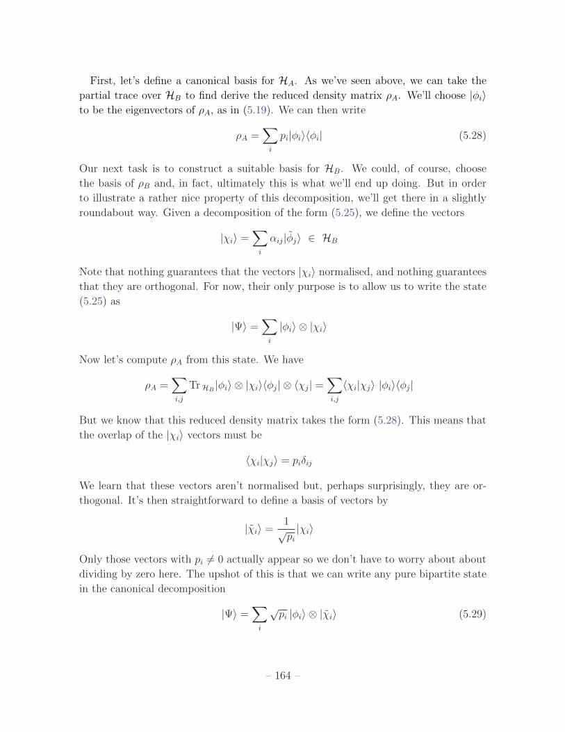
First, let’s define a canonical basis for HA. As we’ve seen above, we can take the

partial trace over HB to find derive the reduced density matrix ⇢A. We’ll choose |�iito be the eigenvectors of ⇢A, as in (5.19). We can then write

⇢A =X

i

pi|�iih�i| (5.28)

Our next task is to construct a suitable basis for HB. We could, of course, choose

the basis of ⇢B and, in fact, ultimately this is what we’ll end up doing. But in order

to illustrate a rather nice property of this decomposition, we’ll get there in a slightly

roundabout way. Given a decomposition of the form (5.25), we define the vectors

|�ii =X

i

↵ij|�ji 2 HB

Note that nothing guarantees that the vectors |�ii normalised, and nothing guarantees

that they are orthogonal. For now, their only purpose is to allow us to write the state

(5.25) as

| i =X

i

|�ii ⌦ |�ii

Now let’s compute ⇢A from this state. We have

⇢A =X

i,j

TrHB |�ii ⌦ |�iih�j|⌦ h�j| =X

i,j

h�i|�ji |�iih�j|

But we know that this reduced density matrix takes the form (5.28). This means that

the overlap of the |�ii vectors must be

h�i|�ji = pi�ij

We learn that these vectors aren’t normalised but, perhaps surprisingly, they are or-

thogonal. It’s then straightforward to define a basis of vectors by

|�ii =1ppi|�ii

Only those vectors with pi 6= 0 actually appear so we don’t have to worry about about

dividing by zero here. The upshot of this is that we can write any pure bipartite state

in the canonical decomposition

| i =X

i

ppi |�ii ⌦ |�ii (5.29)

– 164 –

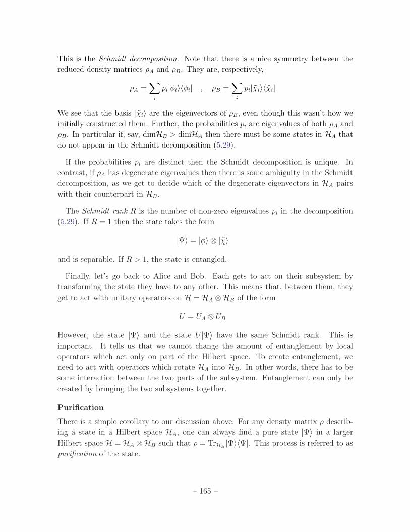
This is the Schmidt decomposition. Note that there is a nice symmetry between the

reduced density matrices ⇢A and ⇢B. They are, respectively,

⇢A =X

i

pi|�iih�i| , ⇢B =X

i

pi|�iih�i|

We see that the basis |�ii are the eigenvectors of ⇢B, even though this wasn’t how we

initially constructed them. Further, the probabilities pi are eigenvalues of both ⇢A and

⇢B. In particular if, say, dimHB > dimHA then there must be some states in HA that

do not appear in the Schmidt decomposition (5.29).

If the probabilities pi are distinct then the Schmidt decomposition is unique. In

contrast, if ⇢A has degenerate eigenvalues then there is some ambiguity in the Schmidt

decomposition, as we get to decide which of the degenerate eigenvectors in HA pairs

with their counterpart in HB.

The Schmidt rank R is the number of non-zero eigenvalues pi in the decomposition

(5.29). If R = 1 then the state takes the form

| i = |�i ⌦ |�i

and is separable. If R > 1, the state is entangled.

Finally, let’s go back to Alice and Bob. Each gets to act on their subsystem by

transforming the state they have to any other. This means that, between them, they

get to act with unitary operators on H = HA ⌦HB of the form

U = UA ⌦ UB

However, the state | i and the state U | i have the same Schmidt rank. This is

important. It tells us that we cannot change the amount of entanglement by local

operators which act only on part of the Hilbert space. To create entanglement, we

need to act with operators which rotate HA into HB. In other words, there has to be

some interaction between the two parts of the subsystem. Entanglement can only be

created by bringing the two subsystems together.

Purification

There is a simple corollary to our discussion above. For any density matrix ⇢ describ-

ing a state in a Hilbert space HA, one can always find a pure state | i in a larger

Hilbert space H = HA ⌦HB such that ⇢ = TrHB | ih |. This process is referred to as

purification of the state.

– 165 –

Everything that we need to show this is in our derivation above. We write the density

matrix in the orthonormal basis (5.28). We then introduce the enlarged Hilbert space

HB whose dimension is that same as the number of non-zero pi in (5.28). The Schmidt

decomposition (5.29) then provides an example of a purification of ⇢.

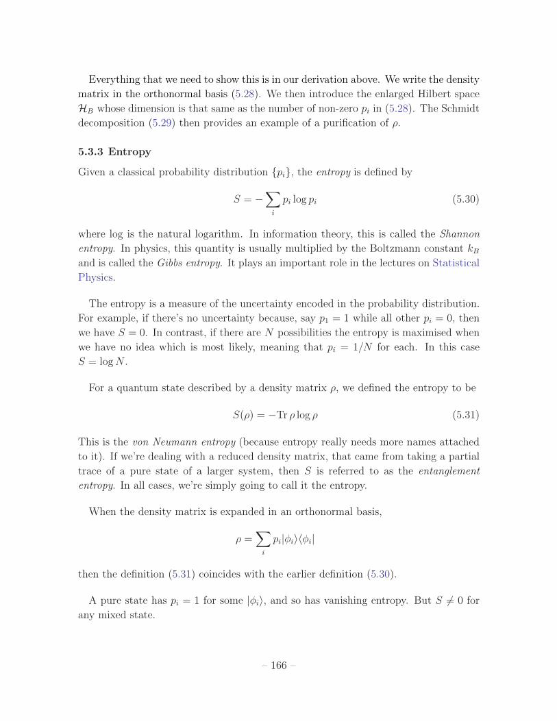
5.3.3 Entropy

Given a classical probability distribution {pi}, the entropy is defined by

S = �X

i

pi log pi (5.30)

where log is the natural logarithm. In information theory, this is called the Shannon

entropy. In physics, this quantity is usually multiplied by the Boltzmann constant kBand is called the Gibbs entropy. It plays an important role in the lectures on Statistical

Physics.

The entropy is a measure of the uncertainty encoded in the probability distribution.

For example, if there’s no uncertainty because, say p1 = 1 while all other pi = 0, then

we have S = 0. In contrast, if there are N possibilities the entropy is maximised when

we have no idea which is most likely, meaning that pi = 1/N for each. In this case

S = logN .

For a quantum state described by a density matrix ⇢, we defined the entropy to be

S(⇢) = �Tr ⇢ log ⇢ (5.31)

This is the von Neumann entropy (because entropy really needs more names attached

to it). If we’re dealing with a reduced density matrix, that came from taking a partial

trace of a pure state of a larger system, then S is referred to as the entanglement

entropy. In all cases, we’re simply going to call it the entropy.

When the density matrix is expanded in an orthonormal basis,

⇢ =X

i

pi|�iih�i|

then the definition (5.31) coincides with the earlier definition (5.30).

A pure state has pi = 1 for some |�ii, and so has vanishing entropy. But S 6= 0 for

any mixed state.

– 166 –

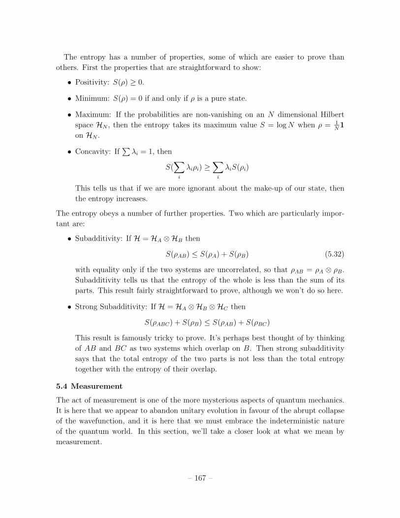
The entropy has a number of properties, some of which are easier to prove than

others. First the properties that are straightforward to show:

• Positivity: S(⇢) � 0.

• Minimum: S(⇢) = 0 if and only if ⇢ is a pure state.

• Maximum: If the probabilities are non-vanishing on an N dimensional Hilbert

space HN , then the entropy takes its maximum value S = logN when ⇢ = 1N 1

on HN .

• Concavity: IfP�i = 1, then

S(X

i

�i⇢i) �X

i

�iS(⇢i)

This tells us that if we are more ignorant about the make-up of our state, then

the entropy increases.

The entropy obeys a number of further properties. Two which are particularly impor-

tant are:

• Subadditivity: If H = HA ⌦HB then

S(⇢AB) S(⇢A) + S(⇢B) (5.32)

with equality only if the two systems are uncorrelated, so that ⇢AB = ⇢A ⌦ ⇢B.Subadditivity tells us that the entropy of the whole is less than the sum of its

parts. This result fairly straightforward to prove, although we won’t do so here.

• Strong Subadditivity: If H = HA ⌦HB ⌦HC then

S(⇢ABC) + S(⇢B) S(⇢AB) + S(⇢BC)

This result is famously tricky to prove. It’s perhaps best thought of by thinking

of AB and BC as two systems which overlap on B. Then strong subadditivity

says that the total entropy of the two parts is not less than the total entropy

together with the entropy of their overlap.

5.4 Measurement

The act of measurement is one of the more mysterious aspects of quantum mechanics.

It is here that we appear to abandon unitary evolution in favour of the abrupt collapse

of the wavefunction, and it is here that we must embrace the indeterministic nature

of the quantum world. In this section, we’ll take a closer look at what we mean by

measurement.

– 167 –

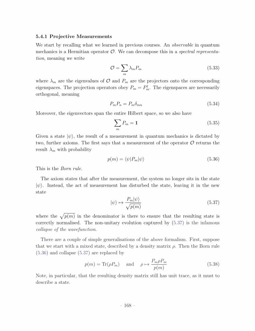
5.4.1 Projective Measurements

We start by recalling what we learned in previous courses. An observable in quantum

mechanics is a Hermitian operator O. We can decompose this in a spectral representa-

tion, meaning we write

O =X

m

�mPm (5.33)

where �m are the eigenvalues of O and Pm are the projectors onto the corresponding

eigenspaces. The projection operators obey Pm = P †

m. The eigenspaces are necessarily

orthogonal, meaning

PmPn = Pm�mn (5.34)

Moreover, the eigenvectors span the entire Hilbert space, so we also haveX

m

Pm = 1 (5.35)

Given a state | i, the result of a measurement in quantum mechanics is dictated by

two, further axioms. The first says that a measurement of the operator O returns the

result �m with probability

p(m) = h |Pm| i (5.36)

This is the Born rule.

The axiom states that after the measurement, the system no longer sits in the state

| i. Instead, the act of measurement has disturbed the state, leaving it in the new

state

| i 7! Pm| ipp(m)

(5.37)

where thep

p(m) in the denominator is there to ensure that the resulting state is

correctly normalised. The non-unitary evolution captured by (5.37) is the infamous

collapse of the wavefunction.

There are a couple of simple generalisations of the above formalism. First, suppose

that we start with a mixed state, described by a density matrix ⇢. Then the Born rule

(5.36) and collapse (5.37) are replaced by

p(m) = Tr(⇢Pm) and ⇢ 7! Pm⇢Pm

p(m)(5.38)

Note, in particular, that the resulting density matrix still has unit trace, as it must to

describe a state.

– 168 –

As an alternative scenario, suppose that we don’t know the outcome of the measure-

ment. In this case, the collapse of the wavefunction turns an initial state | i into a

mixed state, described by the density matrix

| i 7!X

m

p(m)Pm| ih |Pm

p(m)=X

m

Pm| ih |Pm (5.39)

If we don’t gain any knowledge after our quantum system interacts with the measuring

apparatus, this is the correct description of the resulting state.

We can rephrase this discussion without making reference to the original operator

O. We say that a measurement consists of presenting a quantum state with a complete

set of orthogonal projectors {Pm}. These obey (5.34) and (5.35). We ask the system

“Which of these are you described by?” and the system responds by picking one. This

is referred to as a projective measurement.

In this way of stating things, the projection operators take centre stage. The answer

to a projective measurement is su�cient to tell us the value of any physical observable

O whose spectral decomposition (5.33) is in terms of the projection operators {Pm}which we measured. In this way, the answer to a projective measurement can only

furnish us with information about commuting observables, since these have spectral

representations in terms of the same set of projection operators.

Gleason’s Theorem

Where does the Born rule come from? Usually in quantum mechanics, it is simply

pro↵ered as a postulate, one that agrees with experiment. Nonetheless, it is the rule

that underlies the non-deterministic nature of quantum mechanics and given this is

such a departure from classical mechanics, it seems worth exploring in more detail.

There have been many attempts to derive the Born rule from something simpler,

none of them very convincing. But there is a mathematical theorem which gives some

comfort. This is Gleason’s theorem, which we state here without proof. The theorem

says that for any Hilbert space H of dimension dimH � 3, the only consistent way of

assigning probabilities p(m) to all projection operators Pm acting on H is through the

map

p(m) = Tr(⇢Pm)

for some self-adjoint, positive operator ⇢ with unit trace. Gleason’s theorem doesn’t

tell us why we’re obliged to introduce probabilities associated to projection operators.

But it does tell us that if we want to go down that path then the only possible way to

proceed is to introduce a density matrix ⇢ and invoke the Born rule.

– 169 –

5.4.2 Generalised Measurements

There are circumstances where it is useful to go beyond the framework of projective

measurements. Obviously, we’re not going to violate any tenets of quantum mechanics,

and we won’t be able to determine the values of observables that don’t commute.

Nonetheless, focussing only on projection operators can be too restrictive.

A generalised measurement consists of presenting a quantum state with a compete set

of Hermitian, positive operators {Em} and asking: “Which of these are you described

by?”. As before, the system will respond by picking one.

We will require that the operators Em satisfy the following three properties:

• Hermitian: Em = E†

m

• Complete:P

m Em = 1

• Positive: h |Em| i � 0 for all states | i.

These are all true for projection operators {Pm} and the projective measurements

described above are a special case. But the requirements here are weaker. In particular,

in contrast to projective measurements, the number of Em in the set can be larger than

the dimension of the Hilbert space. A set of operators {Em} obeying these three

conditions is called a positive operator-valued measure, or POVM for short.

Given a quantum state | i, we will define the probability of finding the answer Em

to our generalised measurement to be

p(m) = h |Em| i

Alternatively, if we are given a density matrix ⇢, the probability of finding the answer

Em is

p(m) = Tr (⇢Em) (5.40)

At the moment we will take the above rules as a definition, a generalisation of the

usual Born rule. Note, however, that the completeness and positivity requirements

above ensure that p(m) define a good probability distribution. Shortly we will see how

this follows from the more familiar projective measurements.

An Example: State Determination

Before we place generalised measurements in a more familiar setting, let’s first see how

they are may be useful. Suppose that someone hands you a qubit and tells you that

it’s either |" i or it’s |!i = (|" i+ |# i)/p2. How can you find out which state you’ve

been given?

– 170 –

The standard rules of quantum mechanics ensure that there’s no way to distinguish

two non-orthogonal states with absolute certainty. Nonetheless, we can see how well

we can do. Let’s start with projective measurements. We can consider the set

P1 = |" ih"| , P2 = |# ih#|

If the result of the measurement is P1 then we can’t say anything. If, however, the

result of the measurement is P2 then we must have been handed the state |!i becausethe other state obeys P2|" i = 0 and so has vanishing probability of giving the answer

P2. This means that if we’re handed a succession of states | " i and |!i, each with

equal probability, then we can use projective measurements to correctly identify which

one we have 25% of the time.

Generalised measurements allow us to do better. Consider now the set of operators

E1 =1

2|# ih#| , E2 =

1

2| ih | , E3 = 1� E1 � E2 (5.41)

If the result of the measurement is E1, then we must have been handed the state |!i.But, by the same argument, if the result of the state is E2 then we must have been

handed the state | " i. Finally, if the result is E3 then we’ve got no way of knowing

which state we were handed. The upshot is that if we’re handed a succession of states

|" i and |!i, we can use generalised measurements to correctly identify which one we

have 50% of the time.

Generalised Measurements are Projective Measurements in Disguise

The generalised measurements are not quite as novel as they first appear. They can

always be realised as projective measurements in disguise, where the disguise in question

involves some hidden, larger Hilbert space.

Let’s first consider our POVM (5.41). Suppose that when we were handed the states

| " i and |!i, they were actually the first in a pair of qubits, whose full states were

given by

| 1i = |" i ⌦ |" i and | 2i = |!i ⌦ |# i (5.42)

Now these states are orthogonal to each other and, therefore, distinguishable.

We will suppose that the density matrix in the full Hilbert space is separable, meaning

⇢ = ⇢1⌦⇢2. Someone – say, Alice – who has access to both spins can perform projective

measurements in the full four-dimensional Hilbert space, with the resulting probabilities

p(m) = TrH1TrH2(⇢Pm)

– 171 –

What about Bob, who has access only to the first spin? Written in terms of operators

acting on the first qubit, we have

p(m) = TrH1(⇢1Em) where Em = TrH2(⇢2Pm) (5.43)

Here the operators Em form a POVM on H1, the Hilbert space of the first qubit. Both

positivity and completeness follow from the properties of the density matrix ⇢2 and the

projection operators Pm. For example, completeness comes fromX

m

Em = TrH2(⇢2X

m

Pm) = TrH2(12 ⌦ ⇢2) = 12

We learn that the formalism of generalised measurements allows Bob to reproduce any

information that pertains only to the first spin. This is sensible because the original

density matrix ⇢ = ⇢1 ⌦ ⇢2 was separable, which means that there will be no hidden

correlations between the two spins that Alice has access to, but Bob does not.

There are di↵erent ways to arrive at the particular POVM (5.41). For example, we

could consider the situation where we have maximal ignorance about the second spin,

so ⇢2 =1212. Then we can then consider the projectors

P1 = | 1ih 1| , P2 = | 2ih 2| , P3 = 14 � P1 � P2

In this case, the POVM defined by (5.43) coincides with (5.41).

It should be clear that the construction leading to the POVM (5.43) holds more

generally than our two-state system. A projective measurement in any Hilbert space

H1 ⌦H2 reduces to a POVM when taken on separable density matrices. In fact that

converse is also true: any POVM can be realised by projection operators acting on a

larger Hilbert space. This follows from a fairly simple result in linear algebra known as

Naimark’s dilatation theorem (sometimes transliterated from the Russian as Neumark’s

theorem.)

5.4.3 The Fate of the State

The projective measurements that we met in Section 5.4.1 have two ingredients. The

first is the probability that a given result occurs; the second is the fate of the state

after the measurement

p(m) = Tr(⇢Pm) and ⇢ 7! Pm⇢Pm

p(m)(5.44)

For our generalised measurements, we have explained how the probabilities are replaced

by p(m) = Tr(⇢Em). But what happens to the state after the measurement?

– 172 –

We could try to take inspiration from thinking about generalised measurements in

terms of projection operators in an enlarged Hilbert space. We know that

⇢ = ⇢1 ⌦ ⇢2 7!Pm⇢Pm

p(m)) ⇢1 7! TrH2

Pm⇢Pm

p(m)

But there’s no simple way of writing this in terms of the elements of the POVM

Em = TrH2(⇢2Pm). And this is for good reason: the POVM does not include enough

information to tell us the fate of the state.

Instead, we have to define a “square-root” of Em. This is an operator Mm such that

X

m

M †

mMm = Em (5.45)

The Mm need not be Hermitian. Furthermore, these operators are not uniquely de-

termined by (5.45): any unitary transformation Mm ! UMm still obeys (5.45). The

completeness of the POVM means that they obey

X

m

M †

mMm = 1

The choice of Mm is the extra information we need to specify the state after a

generalised measurement. If we perform a generalised measurement and find the answer

Em, then the state becomes

⇢ 7! Mm⇢M †

m

p(m)(5.46)

This new density matrix is Hermitian and has unit trace, as it must.

A full generalised measurement – one in which both the probabilities and the end

state are known – is specified by the set of operators {Mm}, such that Em = M †

mMm

form a POVM. The generalised measurement reduces to the projective measurement

of Section 5.4.1 only when Mm are orthogonal projection operators.

Finally, note that if we make a measurement, but don’t know the result, then the

resulting density matrix is not given by (5.46), but instead by

⇢ 7!X

m

Mm⇢M†

m (5.47)

This generalises our result (5.39) for projective measurements.

– 173 –

Repeated Measurements

The special class of projective measurements enjoys some nice properties that are not

shared by their generalised counterparts. Perhaps the most prominent is what happens

upon repeated measurements.

For projective measurements, if we get a result Pm the first time round, then any

subsequent measurement is guaranteed to give the same result. This result is familiar

from our earlier courses on quantum mechanics: if you measure the spin of a particle

to be up then, as long as the particle is left alone, its spin will continue to be up next

time round.

This property doesn’t hold for generalised measurements. Returning to our POVM

(5.41), a measurement of E1 in the first round does not preclude a measurement of E2

or E1 the next time round.

An Example: Detecting a Photon

The idea of generalised measurement is useful even when our POVM consists of pro-

jection operators. A standard example is the detection of a photon. Before the mea-

surement takes place, either the photon exists |1i or it doesn’t |0i.

A projective measurement (5.44) would tell us that if we detect a photon, then

it’s there to detect again on our next measurement. But that’s not what happens.

Typically when we detect a photon, the photon doesn’t live to tell the tale. Instead, it

is destroyed in the process. This means that whether a photon is seen or not, the end

result is always the same: no photon |0i. In terms of our new generalised measurements,

this can be simply described by the operators

M1 = |0ih0| and M2 = |0ih1|

which corresponds to the POVM

E1 = M †

1M1 = |0ih0| and E2 = M †

2M2 = |1ih1|

In this case, the POVM consists of projection operators. But the collapse of the

wavefunction (5.46) di↵ers from the usual projective measurement. Regardless of the

outcome of the initial experiment, if you now try to repeat it the photon will not be

there.

– 174 –

5.5 Open Systems

In this section we will again consider situations where the full Hilbert space decomposes

into two parts: H = HS ⌦HE. However, we will no longer think of these subspaces as

the far-separated homes of Alice and Bob. Instead, HS will denote the system that we

want to study, and HE will denote the surrounding environment.

Here the environment is typically a vast Hilbert space which we have no way of

understanding completely. In this sense, it plays a similar role to the thermal baths

that we introduce in statistical physics. When performing an experiment on a quantum

system, much of the challenge is trying to shield it from the environment. However, in

many cases this is not possible and there will be coupling between HS and HE. We

then say that HS is an open system. The purpose of this section is to understand how

such open quantum systems behave.

5.5.1 Quantum Maps

We will assume that the combined system+environment is described by a pure state

| i. We’ve seen in Section 5.3.2 that, after tracing over HE, the system we care about

is typically described by a reduced density matrix

⇢ = TrHE | ih |

We would like to understand how this density matrix evolves.

The state | i evolves by a unitary operator U(t) acting on the full Hilbert space H.

The story that we are about to tell only works if, at time t = 0, the two systems lie in

a separable state,

| 0i = | i ⌦ |�i (5.48)

This means that the original density matrix ⇢0 = | ih | describes a pure state on HS.

We now look at how this density matrix evolves. We have

⇢(t) = TrHE U(t)| 0ih 0|U †(t) =X

m

hm|U(t)| 0ih 0|U †(t)|mi

with |mi a complete basis for HE. This encourages us to define a set of operators on

HS, given by

Mm(t) = hm|U(t)|�i = TrHE

⇣U(t)|�ihm|

⌘(5.49)

– 175 –

The unitarity of U(t) translates into a completeness condition on the operators Mm(t),X

m

M †

m(t)Mm(t) =X

m

h�|U †(t)|mihm|U(t)|�i = 1

We see that the original density matrix on HS evolves as

⇢(t) =X

m

Mm(t) ⇢0 M†

m(t) (5.50)

In general, this will describe the evolution from a pure state to a mixed state. This

evolution is not, in general, reversible.

A quick comment: this evolution takes the same general form as the measurement

process (5.47), at least if we don’t gain any knowledge about the result of the measure-

ment. This is not coincidence. A measuring apparatus is a macroscopic system that

becomes entangled with the quantum state. In this sense, it plays a similar role to the

environment in the discussion above.

In contrast, if we read o↵ the result of a measurement, then the resulting state is

described by (5.46); this does not take the form (5.50).

Kraus Representation Theorem

Above, we have derived the evolution (5.50) in a rather simple example. However, it

turns out that this form has more general applicability. Consider a density operator

HS which evolves by the map

⇢ 7! L[⇢]

Such a map is sometimes called a superoperator (because it maps operators to operators,

rather than states to states). We will require some special properties of our map, most

of which are inherited from the properties of the density matrices listed in Section 5.3

• Linearity: L[a⇢1 + b⇢2] = aL[⇢1] + bL[⇢2].

• Hermiticity Preserving: ⇢ = ⇢† ) L[⇢] = L[⇢]†.

• Trace Preserving: TrL[⇢] = Tr ⇢.

• Complete Positivity. This one requires some explanation. It is natural to insist

that the map is positive, so that L[⇢] � 0 whenever ⇢ � 0. However, this is

not su�cient. Instead, we require the stronger statement that the map L ⌦ 1E

is positive on any extension of the Hilbert space HS to HS ⌦ HE. This is the

statement of complete positivity. It ensures that the map L⌦1E will take a valid

density matrix on the composite system to another density matrix.

– 176 –

A superoperator obeying these conditions is called a trace preserving, completely pos-

itive (TPCP) map, with the first two conditions taken for granted. In the quantum

information community, this map is referred to as a quantum channel.

The Kraus representation theorem (which we do not prove here) states that any

quantum map, obeying the four conditions above, can be written as

L[⇢] =X

m

Mm⇢M†

m withX

m

M †

mMm = 1 (5.51)

In this framework, the Mm are called Kraus operators. They are not unique. The

number of Kraus operators in the quantum map does not exceed dim(HS)2.

You might wonder why the collapse of the wavefunction (5.46) fails to take the Kraus

form (5.51). It is because the map is not linear: the probability p(m) which normalises

the resulting density matrix itself depends on ⇢ through (5.40).

5.5.2 Decoherence

In this section, we explore some simple examples of quantum maps. We’ll use these toy

models to highlight some important and general features that emerge when quantum

systems interact with an environment.

Phase-Damping

We will take the quantum system HS to be our trusty qubit. Meanwhile, we will model

the environment HE by a three-state system, spanned by |0i, |1i and |2i. Consider thefollowing unitary evolution

U |" i ⌦ |0i = |" i ⌦ (p1� p |0i+pp |1i)

U |# i ⌦ |0i = |# i ⌦ (p1� p |0i+pp |2i) (5.52)

This means that our qubit interacts with the environment with probability p, changing

the initial state |0i into either |1i or |2i depending on the state of the qubit. Note,

however, that the state of the qubit is unchanged by this interaction. So this model

describes a system in which the energies needed to change the qubit are substantially

larger than those needed to change the environment.

If you want a specific picture in mind, you could think of the qubit as a simplified

model for a heavy dust particle which, in this case, can only sit in one of two positions

|" i or |# i. The environment could be a background bath of photons which scatter o↵

this dust particle with probability p.

– 177 –

The Kraus operators for this quantum map are easily calculated. Using (5.49), they

are given by

M0 = h0|U |0i =p

1� p1

M1 = h1|U |0i = pp |" ih"| (5.53)

M2 = h2|U |0i = pp |# ih#|

which can be checked to obey the required completeness conditionP

m M †

mMm = 1.

The state of the qubit, described by a density matrix ⇢, then evolves as

⇢ 7! L[⇢] =X

m

M †

m⇢Mm = (1� p) ⇢+ p|0ih0|⇢|0ih0|+ p|1ih1|⇢|1ih1|

= (1� 1

2p)⇢+

1

2p�3⇢�3

We can see the essence of this quantum map if we write the density matrix in terms of

components

⇢ =

⇢00 ⇢01

⇢10 ⇢11

!7!

⇢00 (1� p)⇢01

(1� p)⇢10 ⇢11

!

We learn that the o↵-diagonal components are suppressed by the evolution. It is

these o↵-diagonal elements which encode possible superpositions of |" i and |# i. The

interactions with the environment — or, more precisely, the resulting entanglement

with the environment — means that these o↵-diagonal elements are reduced under

time evolution. This process is known as decoherence; it is the evolution of a pure state

into a mixed state through interactions with the environment.

We can get a better sense of this if we look at successive maps. This is a little subtle

because it’s not obvious when we can apply successive Kraus operators (5.53). We

will discuss this in more detail in Section 5.5.3, but for now we simply look at what

happens.

We define the probability of scattering per unit time to be �. Then, in time �t, we

have p = ��t ⌧ 1. After a total time t = N�t, the o↵-diagonal terms in the density

matrix are suppressed by

(1� p)N = (1� �t/N)N ⇡ e��t (5.54)

Suppose that we initially prepare our qubit in a state

| i = ↵|" i+ �|# i |↵|2 + |�|2 = 1

– 178 –

Then after time t, the density matrix becomes

⇢(t) =

|↵|2 ↵�? e��t

↵?�e��t |�|2

!

We see that these o↵-diagonal components decay exponentially quickly, with the system

ultimately settling down into a mixed state. The choice of preferred basis |" i, |# i canbe traced to the form of the original interaction (5.52)

To flesh this out a little, let’s return to our interpretation of this model in terms of

a heavy dust particle which can sit in one of two positions, |" i = |x+i or |# i = |x�i.We may, of course, choose to place this particle in a superposition

| i = ↵|x+i+ �|x�i

and hope to measure this superposition in some way. This, of course, is what happens

in the double-slit experiment. However, decoherence makes this di�cult. Indeed, if

the particle takes time t� ��1 to traverse the double slit experiment then all the hint

of the superposition will be washed out. Furthermore, ��1 is typically a very short

timescale; it is the rate at which a single photon scatters o↵ the particle. This can be

much much shorter than the rate at which the classical properties of the particle – say

its energy – are a↵ected by the photons.

There is one final important lesson to take away from this model. It explains why

the decoherence occurs in the position basis |x±i rather than say, (|x+i ± |x�i)/p2.

This is because the interactions (5.52) are local.

The locality of interactions is one of the key features of all physical laws; indeed, it

underlies the idea of quantum field theory. Combined with decoherence, this explains

why we only see our favourite pets in the state |alivei or |deadi. Interactions with the

environment mean that it is overwhelmingly unlikely to observe Schrodinger’s cat in

the state | i = (|alivei± |deadi)/p2.

Amplitude Damping

Our second example will not give us further insight into decoherence, but instead

provides a simple model for the decay of an excited atom. (A more detailed look at the

dynamics underling this can be found in Section 4.4.3.) Consider a two-state atomic

system. If the atom is in the ground state | " i then nothing happens, but if atom is

in the excited state | # i then it decays with probability p emitting a photon in the

– 179 –

process, so that the environment changes from |0i to |1i. This is captured by the

unitary evolution

U |" i ⌦ |0i = |" i ⌦ |0iU |# i ⌦ |0i =

p1� p |# i ⌦ |0i+pp |" i ⌦ |1i)

The resulting Kraus operators are

M0 = h0|U |0i = |"ih"|+p1� p|# ih # | , M1 = h1|U |0i = pp |" ih # |

This time the quantum map is given by

⇢ =

⇢00 ⇢01

⇢10 ⇢11

!7!

⇢00 + p⇢11

p1� p ⇢01

p1� p ⇢10 (1� p)⇢11

!

If, as previously, we can think about performing this map successive time, with the

probability for decay p related to the lifetime ��1 of the excited state through (5.54)

then we find the time-dependent density matrix given by

⇢(t) =

⇢00 + (1� e��t)⇢11 e��t/2⇢01

e��t/2⇢10 e��t⇢11

!

Interestingly, as t!1, the system ends up in the pure state |" i, regardless of whateversuperposition or mixed state it started in. On the one hand this is not surprising: it

is simply the statement that if we wait long enough the atom will surely have decayed.

Nonetheless, it does provide a simple example in which quantum maps can take a mixed

state to a pure state.

5.5.3 The Lindblad Equation

Usually in physics, the most powerful way to describe the evolution of a system is

through a di↵erential equation. For a closed quantum system in a pure state, the

relevant equation is the Schrodinger equation. For a closed quantum system in a mixed

state, it is the Liouville equation (5.21)

~ @⇢@t

= �i[H, ⇢]

where the density matrix ⇢ is an operator on HS. Here we would like to derive the

analogous equation for an open quantum system, where HS is also coupled to an envi-

ronment HE.

– 180 –

It is not at all clear that such an equation will exist. Knowledge of the density

matrix ⇢ on HS at some time will not, in general, be su�cient to tell you how the

density matrix will behave in the future. The problem is not just that the environment

can a↵ect our system — that, after all is what we’re trying to model. The problem is

more one of memory.

As time progresses, the system changes the environment. Our concern is that these

changes accumulate, so that the environment starts to a↵ect the system in di↵erent

ways. In this sense, the environment can act as a memory, where the state of the

system in the future depends not only on the present state, but on its entire history.

These kind of situations are complicated.

We’ve already seen a hint of this in our earlier work. Recall that when we first

looked at quantum maps, we assumed that the initial state (5.48) was separable, with

no correlations between HS and HE. Had we included these correlations, we would not

have found such a simple, linear quantum map. Yet, such correlations inevitably build

with time, meaning that we should be careful about performing successive quantum

maps. This is a manifestation of the memory of the environment.

To make progress, we will restrict ourselves to situations where this memory does

not last. We will consider the environment to be vast, similar to the heat reservoirs

that we use in statistical mechanics. We assume that correlations between the system

and the environment are lost over a certain time scale. We will denote this time scale

by ⌧ , and seek an equation which dictates the dynamics of ⇢ on timescales t� ⌧ .

Our starting point is the quantum map (5.50),

⇢(t+ �t) =X

m

Mm(t+ �t) ⇢(t)M †

m(t+ �t) (5.55)

We will take �t to be small, as if we were dealing with usual calculus of infinitesimals.

But we should bear in mind that really we want �t� ⌧ . For this equation to hold, we

must have one Kraus operator — say M0 — to take the form M0 = 1 + O(�t). The

remaining operators should be Mm ⇠ O(p�t). We write

M0 = 1+1

~(K � iH)�t , Mm =1p~Lm

p�t m = 1, 2, . . .

where both H and K are chosen to be Hermitian matrices. These Kraus operators

must obey the completeness relation (5.51),X

m=0

M †

mMm = 1 ) 2K +X

m=1

L†

mLm = O(�t2)

– 181 –

We therefore write

K = �1

2

X

m=1

L†

mLm

Plugging these expressions into the quantum map (5.55), and keeping only terms of

order �t, we get our final result

~ @⇢@t

= �i[H, ⇢] +X

m=1

Lm⇢L

†

m �1

2L†

mLm⇢�1

2⇢L†

mLm

�

This is the Lindblad equation. It should be thought of as a quantum version of the

Fokker-Planck equation that is described in the lectures in Kinetic Theory. We see that

the evolution is governed not just by the Hamiltonian H, but also by further Lindblad

operators Lm which capture the interaction with the environment. The presence of the

final two terms ensures that d(Tr ⇢)/dt = 0, as it should for a density matrix.

The Increase of Entropy

Something particularly nice happens when the Lindblad operators are Hermitian, so

Lm = L†

m. In this case, the entropy increases. The von Neumann entropy is defined as

(5.31)

S(⇢) = �Tr ⇢ log ⇢

Its change in time is given by

dS

dt= �Tr

✓@⇢

@t(1 + log ⇢)

◆= �Tr

✓@⇢

@tlog ⇢

◆

Inserting the Lindblad equation, we see that the first term vanishes, courtesy of the

fact that [⇢, log ⇢] = 0. We’re left with

~dSdt

=X

m

Tr [(Lm⇢Lm � LmLm⇢) log ⇢]

To proceed, we decompose the density matrix ⇢ in terms of its eigenvectors

⇢ =X

i

pi|�iih�i|

and take the trace by summing over the complete basis |�ii. We have

~dSdt

=X

m

X

i

h�i|(Lm⇢Lm � LmLm⇢)|�ii log pi

=X

m

X

i,j

h�i|Lm|�jih�j|Lm|�ii(pj � pi) log pi

=1

2

X

m

X

i,j

|h�i|Lm|�ji|2(pj � pi)(log pi � log pj)

– 182 –

where, in going to the final line, we took advantage of the anti-symmetric properties of

the middle line under the exchange of i and j. However, the expression (x� y)(log x�log y) is positive for all values of x and y. (This same fact was needed in the proof of

the H-theorem which is the classical analog of the result we’re deriving here.) We learn

that

~dSdt� 0

– 183 –