116

4.5 Recursion

One of the most powerful programming techniques involves a function callingitself; this is called recursion. It is not immediately obvious that this is useful;take that on faith for now and concentrate first on how to make recursion work.The utility should become apparent as you see it in action.

Here is a complete program that will serve as our first example of recursion:

def F a c t o r i a l ( n ) :i f n <= 1 :

return 1else :

return n∗ F a c t o r i a l ( n−1)

def main ( ) :print ( F a c t o r i a l ( 4 ) )

main ( )

Program 4.5.1: The recursive Factorial function

Before we think about what the program does, let’s concentrate on theFactorial () function:

def F a c t o r i a l ( n ) :i f n == 1 :

return 1else :

return n∗ F a c t o r i a l ( n−1)

Can we see what this function will return for Factorial (1)? Sure; if n is 1 thenthe first line: if n == 1 is True so Factorial (1) returns 1.

What about Factorial (2)? Well, if n is 2 then the test n==1 fails and thefunction returns 2∗ Factorial (1). But we just saw that Factorial (1) returns 1,so Factorial (2) must return 2.

Factorial (3)? If n is 3 then again n==1 is False and the function returns3∗ Factorial (2). We just saw that Factorial (2) returns 2, so Factorial (3) mustreturn 6.

One more time. If n is 4 then n==1 is False and the function returns4∗ Factorial (3). We just saw that Factorial (3) returns 6, so Factorial (4) mustreturn 24. If we now look at our program, in main() it prints Factorial (4), sothe program prints the number 24 and halts.

Of course, you have surely noticed that Factorial (2) is 2, which is 2∗1,Factorial (3) is 6, which is 3∗2∗1, and Factorial (4) is 24, which is 4∗3∗2∗1. Ourfunction is indeed computing what mathematicians call the Factorial () function.Factorial (n) is the product of the first n positive integers. This should make

4.5. RECURSION 117

sense: if Factorial (n−1) is the product of the first n−1 positive integers, wehave defined the function so that Factorial (n) is n times the product of the firstn−1 positive integers, and that is the product of the first n positive integers.

Notice that the code for our Factorial () starts with an if statement oneone of whose branches the function returns without calling itself. The valuesfor which a function returns without recursing are called base cases. We com-puted Factorial (4) by starting at the base case Factorial (1) and working upuntil we reached the Factorial (4) case. Can we go the other way – computingFactorial(4) the way the computer does?

We start with a definition straight from the function:

F a c t o r i a l (4)=4∗ F a c t o r i a l ( 3 )We don’t yet know the value of Factorial (3), so we remember where we are andstart a new computation:

F a c t o r i a l (4)=4∗ F a c t o r i a l ( 3 )F a c t o r i a l (3)=3∗ F a c t o r i a l ( 2 )

We don’t know the value of Factorial (2), so again we remember where we areand start a new computation:

F a c t o r i a l (4)=4∗ F a c t o r i a l ( 3 )F a c t o r i a l (3)=3∗ F a c t o r i a l ( 2 )

F a c t o r i a l (2)=2∗ F a c t o r i a l ( 1 )Finally, we do know the value of Factorial (1):

F a c t o r i a l (4)=4∗ F a c t o r i a l ( 3 )F a c t o r i a l (3)=3∗ F a c t o r i a l ( 2 )

F a c t o r i a l (2)=2∗ F a c t o r i a l ( 1 )F a c t o r i a l (1)=1

We can now work our way back up. Since we know Factorial (1)=1 we cancompute Factorial (2):

F a c t o r i a l (4)=4∗ F a c t o r i a l ( 3 )F a c t o r i a l (3)=3∗ F a c t o r i a l ( 2 )

F a c t o r i a l (2)=2∗ F a c t o r i a l (1)=2∗1=2F a c t o r i a l (1)=1

and now we can compute Factorial (3):

F a c t o r i a l (4)=4∗ F a c t o r i a l ( 3 )F a c t o r i a l (3)=3∗ F a c t o r i a l (2)=3∗2=6

F a c t o r i a l (2)=2∗ F a c t o r i a l (1)=2∗1=2F a c t o r i a l (1)=1

and finally

F a c t o r i a l (4)=4∗ F a c t o r i a l (3)=4∗6=24F a c t o r i a l (3)=3∗ F a c t o r i a l (2)=3∗2=6

F a c t o r i a l (2)=2∗ F a c t o r i a l (1)=2∗1=2F a c t o r i a l (1)=1

118

Follow the black arrows down into the recursion, then the red arrows back out.You can imitate the way a computer executes any recursive function in this

way. It becomes a bookkeeping problem – the difficulty is just in keeping trackof what has been evaluated and where you are in the computation.

Notice that our recursive factorial function started with an if–statement.This is true of almost all recursive functions. The first question to ask is whetherthe argument to the function is one of the base cases. If so we can just returnthe answer; it is only when the argument is not a base case that we need torecurse. Notice also that in order for the recursive function call to terminate,the argument in the recursive call must be closer to a base can than the initialargument was. To compute Factorial (n) we recurse on Factorial (n−1). If n islarger than 1, n−1 is closer to the base case of 1 than n is. On the other hand,if n is not positive then n−1 moves farther away from 1, and as a result theFactorial () function never halts if you give it a non-positive argument.

The aspect of recursion that students find hardest is writing recursive func-tions. This almost seems like magic. Here is a way to think about the process:

• Find the base case. This usually tells you what the parameter of thefunction should be. Start the recursive function with an if-statement thatdescribes how to perform the computation for the base case.

• Handle the recursive case. Describe how to perform the computation ifthe parameter is not the base case, in terms of parameters that would becloser to the base case.

• Be sure that the recursion always works down to one of the base cases.

Example 1:Write a recursive function that returns the length of a string.Strings can be long: ”Marvin Krislov is President of Oberlin College”, or short:”bob”. Short ones seem easier to deal with than long ones. The shortest possi-ble string is ””, the empty string. We’ll take that as our base case. If the stringis empty is our base case, our recursive parameter must be the string and ourfunction starts

def l e n g t h ( s t r i n g ) :i f s t r i n g == ”” :

return 0else :

4.5. RECURSION 119

Now we need to handle the recursive cases: the cases where the base case doesnot apply. This means we have a string whose length is not 0. The length can’tbe negative, so our string must have positive length. To make use of recursion,we want to find its length in terms of the lengths of strings closer to the basecase: i.e., string with shorter length. With a little thought you can see thatthe length of the string is 1 more than it would be if we removed one letter.One way to remove a letter is to make use of our string indexing operations:string [1:] consists of all of the letters of string after the first. We add this toour code with one line:

def l e n g t h ( s t r i n g ) :i f s t r i n g == ”” :

return 0else :

return 1 + l e ng t h ( s t r i n g [ 1 : ]

That is our function. Does it always lead us to a base case? Sure; for anystarting string we remove one letter at a time until we get to the empty string:

Example 2: Write a recursive function to make the Fibonacci sequence 0,1,1,2,3,5,8,13.....The Fibonacci sequence is easy to describe in English: it starts with 0 and 1,and then every subsequent number is the sum of the two previous numbers.Since ”starts with 0 and 1” is a statement about position in the sequence, wewill write a function Fib(n), where n refers to position in the sequence: Fib(0) isthe first number in the sequence, Fib(1) is the second, and so forth. Our Englishdescription of the problem gives us two base cases:

def Fib ( n ) :i f n==0:

return 0e l i f n==1:

return 1else :

We will look later at whether we actually need both of the base cases. OurEnglish description is easy to translate into the recursive case of our function.The description says ”every subsequent number is the sum of the two previousnumbers.” If n is the index of the number we are currently calculating, theindexes of the two previous numbers are n−1 and n−2. In other words, our

120

description says Fib(n)=Fib(n−1)+Fib(n−2). We translate this into code bymaking the right hand side the value that we return:

def Fib ( n ) :i f n==0:

return 0e l i f n==1:

return 1else :

return Fib (n−1)+Fib (n−2}

It is easy to see that we need both of our base cases. The calculation ofFib(2 uses both of them: Fib(2)=Fib(1)+Fib(0). If we omitted one of themas a base case and tried to calculate it recursively we would get into trou-ble. For example, if we tried to calculate Fib(1) recursively we would getFib(1)=Fib(0)+Fib(−1)=0+Fib(−2)+Fib(−3)=... and this clearly will never ter-minate. Are our two base cases enough? Yes; the calculation works downthrough even numbers and odd numbers and our base cases of 0 and 1 termi-nate both the evens and the odds.

Here is a sample calculation with our function

Example 3: Write a recursive function to solve the Towers of Hanoi puzzleTowers of Hanoi is a puzzle game invented in1883 by the French mathematicianEdouard Lucas. In this game there are three ”towers” or vertical sticks thatcan hold a set of concentric disks. At the start of the game the disks are all onone tower, in order of decreasing size with the largest disk at the bottom andthe smallest at the top:

4.5. RECURSION 121

The goal of the game is to move all of the disks from their starting tower toanother tower, using the following three rules:

1. Only one disk can be moved at a time.

2. Only the top disk on a tower can be moved.

3. A disk can only be placed on an empty tower or on a larger disk, neveron a smaller disk.

Lucas’s game included a story, supposedly taken from the writings of aneminent Chinese monk who lived in Hanoi, that there is a temple in India wherethe Brahmin monks are working on a version of this puzzle with 64 golden disks.A prophecy claims that when the monks finish solving the puzzle the world willcome to an end.

122

Just for fun, here is the cover of the box containing Lucas’s first version ofthe puzzle:

Now we need to find a solution. As usual we’ll start thinking about basecases. An easy setup to solve is when we have only one disk on the startingtower; we can move that to either of the other towers in one step. However,an even easier setup is when we have no disks at all; we can solve that withoutdoing anything! Both of these cases refer to the number of disks on the startingtower. If you think about it, the only difference in two distinct starting statesis the number of disks they contain. So we’ll include the number of disks asa parameter on our Hanoi() function. Since our case with 0 disks requires nowork, we can start the function as follows

4.5. RECURSION 123

def Hanoi ( n ) :#So l v e s Towers o f Hanoi w i th n d i s k s on the s t a r t i n g toweri f n>0:

This, however, is not enough. We need to know not just how many disks are onthe starting tower, but the situations with the other towers as well. Once weare into the recursion we need to move disks not just from the starting tower,but from all three towers. So we will include all three towers as parameters:

def Hanoi (n , source , d e s t i n a t i o n , f r e e ) :# Moves n d i s k s from the ” sou r c e ” tower to the# ” d e s t i n a t i o n ” tower , making use o f the ” f r e e ” tower .i f n>0:

Now we are rolling. We need to express how to move n disks from the sourceto the destination in terms of moving small numbers of disks from one tower toanother. This is easy:

1. Move n−1 disks from the source tower to the free tower.

2. Move 1 disk, the largest, from the source tower to the destination.

3. Move n−1 disks from the free tower to the destination.

For example, suppose we start with 3 disks on tower A, the other towers empty:

We will think of A as our source tower, B as our destination and C as free. Wefirst recursively move 2 disks from A to C:

Next we move the largest disk from A to B:

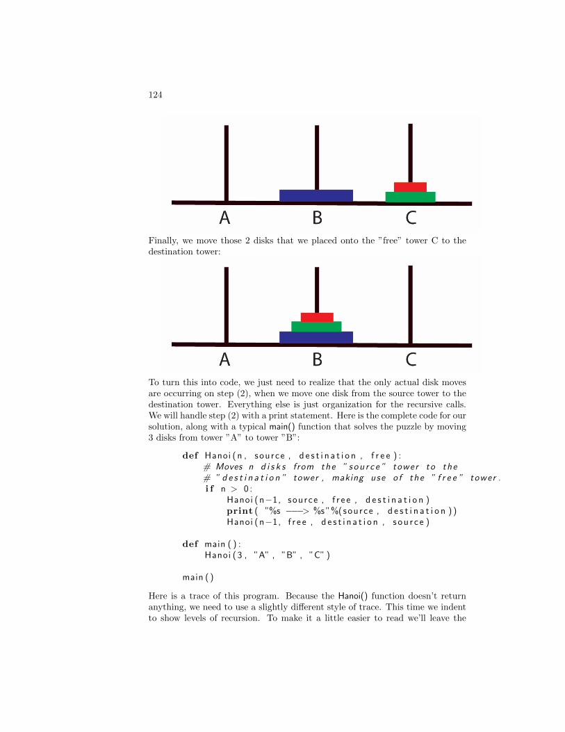
124

Finally, we move those 2 disks that we placed onto the ”free” tower C to thedestination tower:

To turn this into code, we just need to realize that the only actual disk movesare occurring on step (2), when we move one disk from the source tower to thedestination tower. Everything else is just organization for the recursive calls.We will handle step (2) with a print statement. Here is the complete code for oursolution, along with a typical main() function that solves the puzzle by moving3 disks from tower ”A” to tower ”B”:

def Hanoi (n , source , d e s t i n a t i o n , f r e e ) :# Moves n d i s k s from the ” sou r c e ” tower to the# ” d e s t i n a t i o n ” tower , making use o f the ” f r e e ” tower .i f n > 0 :

Hanoi (n−1, source , f r e e , d e s t i n a t i o n )print ( ”%s −−−> %s”%(source , d e s t i n a t i o n ) )Hanoi (n−1, f r e e , d e s t i n a t i o n , s ou r c e )

def main ( ) :Hanoi (3 , ”A” , ”B” , ”C” )

main ( )

Here is a trace of this program. Because the Hanoi() function doesn’t returnanything, we need to use a slightly different style of trace. This time we indentto show levels of recursion. To make it a little easier to read we’ll leave the

4.5. RECURSION 125

quotes off the strings. At the top level Hanoi(3,A,B,C) is performed with 3 calls:

Hanoi (2 ,A,C ,B)print A −−−> BHanoi (2 ,C ,B,A)

We write those three at the same indentation level, then go in a further level forthe recursive calls for Hanoi(2,A,C,B) and Hanoi(2,C,B,A). Here is the resultingtrace:

We will walk through the 7 steps. We start with

The first move is A—>B:

126

Then A—>C:

B—>C:

A–>B:

C—>A:

4.5. RECURSION 127

C—>B:

And finally A–>B:

It is not hard to show that solving the puzzle with n disks takes 2n − 1 moves.Those 64 disks the monks are supposedly moving need about 1019 individualmoves. There are about 3 ∗ 107 seconds in a year, so if the monks were movingone disk per second it would take roughly 3 ∗ 1011 years to solve the puzzle.Sadly, astrophysicists currently estimate that the sun will burn out in on 5∗109

years, so the monks really need to speed up.