43

44 Uncertainty in remote sensing classificationsUncertainty in remote sensing classifications

“...Variation seems inevitable in nature (...) It follows that it is necessary to have somesimple methods of describing patterns of variation. Statisticians have developed suchmethods...”

Grant & Leavenworth (1988) - “Statistical Quality Control”

4.1 Introduction

The classification of remotely sensed data by means of digital automated featureextraction is attended by an often undefined amount of uncertainty concerning theproperties of the extracted features (Kretsch & Mikhail, 1990). This uncertaintycauses spatial and non-spatial variability in the processing outcomes that, in turn,could hamper a sound decision-making procedure. Here, decision-making refers tothe eventual use of the processed (classified or not) remotely sensed data – not to theclassification rule itself. Smith et al. (1991) provide examples that illustrate therelevance of knowledge about this variability, which allows for more well balanceddecisions including cost-benefit considerations. With respect to remote sensingclassifications, Middelkoop et al. (1989) state that “...the maximum likelihood rule (...)can include weight factors for the cost of incorrect decisions and the benefit of correct ones...”Within this context, the issue of data quality has been put on the scene in section 1.4.But what exactly does this quality involve and what is its relationship, if any, withuncertainty, error and accuracy?

The aim of this chapter is to remove possible confusion as far as intermixedterminology is concerned. This is not achieved by simply providing definitions only.By retrieving the sources from which the imperfections in remotely sensed dataoriginate and by revealing the mechanisms by which they are propagated duringprocessing, the distinctions between different concepts are best elucidated.

Furthermore, the concept of uncertainty is considered in view of the two maximumposterior classification rules that have been discussed in the previous chapter. Fromthis, strategies are designed to deal with this inherent characteristic of the consideredgeographical data.

44

4.2 On defining some relevant concepts

For a start, a number of definitions is presented in an attempt to produce order out ofchaos.• Error. According to Heuvelink (1993) error can be described as “...the difference

between reality and our representation of reality; it includes not only ‘mistakes’ or ‘faults’but also the statistical concept of ‘variation’...”, thereby linking up with Burrough(1986). Errors evoke negative, unfavourable associations; “...error is a bad thing...”as Chrisman (1991) notices. But, on the other hand, in everyday language the useof the term error suggests that they can be corrected and hence don’t need to be toodisastrous after all. As Chrisman (1989) points out, this may be the case forblunders (the easy-to-detect-and-remove mistakes in Heuvelink’s (1993) definition)but it certainly fails to account for the more subtle, random errors that are beingdealt with in a statistical way. In the literature, a number of error taxonomies havebeen proposed whose aim is to improve understanding of the way in which errorsare introduced and propagated (see next section).

• Accuracy. Accuracy is often described as “...the closeness of results of observations,computations or estimates to the true values or the values accepted as being true...” (agi,1991). In a statistical sense, this can be interpreted as the degree with which anestimated mean differs from the true mean (Burrough, 1986). In order to assessaccuracy, a source of higher accuracy is needed as a representation of the true orreal world, “...but the ‘truth’ can never be known...” (Drummond, 1995). Considerfor example the comparison of a remote sensing classification with a ground truthmap during an accuracy assessment procedure. The accuracy of the classificationcan be affected by errors, but the reference - ground truth - data itself (the“modelled” truth) could be error-prone as well. Their obvious relationshipnotwithstanding, error and accuracy are clearly not the same thing, as Unwin(1995) contends correctly. “...Accuracy differs conceptually from error in measuringdiscrepancy from a model; error measures discrepancy from the truth...” (Buttenfield &Beard, 1994). Accuracy can be distinguished in a positional and attributecomponent, in accordance with the respective errors that could arise ingeographical data.

• Precision. Precision is “...the exactness with which a value is expressed, whether thevalue be right or wrong...” (agi, 1991). Unwin (1995) expresses himself in moreconcrete terms by defining it as “...the number of decimal places or significant digits ina measurement...” High precision doesn’t necessarily relate to high accuracy;instead, it is even possible to characterise data in a very precise, but completelyerroneous way!

• Quality. Quality is defined as “...fitness for use...” by Chrisman (1984). Its relevanceis discerned by a number of digital spatial data standards, e.g. the American SpatialData Transfer Standard (sdts) issued by the United States Geological Survey(usgs) in 1992. In order to enable a self-contained exchange of spatial databetween heterogeneous computer systems it is required that - among others - datasets be described according to a metadata structure, involving quality issues as well.Its aim is to provide users with sufficient information in order to evaluate thefitness for a particular application. Moellering (1987), in his well-known report inpreparation to the completion of the sdts, advocates a “truth in labelling”

45

approach, meaning that information about uncertainty is made available withoutassigning a predefined, a priori value judgement. Quality, therefore, is a relativeconcept dependent on the pursued aims and the considered context. It is this lackof an absolute meaning that makes quality a difficult concept to work with directly.Instead, a number of quality components has been proposed that clearly reveal theextensiveness of the concept. Guptill & Morrison (1995) offer an excellentcollection of papers on each of these components. Later on in this chapter moreattention will be paid to these quality components because of the prominentposition that they occupy in spatial data standards.

• Uncertainty. Increasingly, the concept of uncertainty is introduced whendiscussing the imperfections inherent to geographical data handling. Quality maybe a good starting point for summarising and describing a lot of - different - datacharacteristics affecting the appropriateness of that data for a particular purpose,but it is also a very general and comprehensive concept. Goodchild (1995) arguesthat uncertainty is “...generic and reasonably value-free, and implies nothing aboutsources or whether they can be corrected...” This is in flat contradiction to theobservation made by Heuvelink (1993) that uncertainty is “...synonymous toerror...” In this thesis, uncertainty is used as a useful concept to express theinability to be confident of, and knowledgeable about the truth value of a particulardata characteristic; uncertainty indicates a “...lack of knowledge...” (Stephanou &Sage, 1987). The argument that MacEachren (1995) brings forward to supporthis move to abandon the idea of uncertainty, namely that it bears a negative load, israther weak; instead of adopting certainty as a complementary (and more positive)concept, he advocates the use of reliability. This concept, however, is commonlyused in a more narrow statistical sense, referring to the repeatability andverifiability of measurement and processing results. In an earlier paper,MacEachren (1992) elucidates the distinction between quality and uncertainty ashe emphasises the issue of variability over both space and time, and withincategories. In case of a remote sensing classification, the aggregation of thematicland cover classes causes uncertainty, the possible high quality of the separateclasses notwithstanding. To make it even more complicated it is stated that theimpact of this uncertainty is dependent on the user’s perception of the real world.A simple, almost “binary” worldview (urban versus non-urban area) allows formore general categories whose validity is not disturbed by within-class variability.

4.3 Sources of uncertainty in remotely sensed data

During the life cycle of remotely sensed data, uncertainties are introduced andpropagated in an often unknown way. In this respect, these data are not any differentfrom other spatial data except for the fact that the acquisition and processingtechniques used can be held responsible for specific types of uncertainty. Areconstruction of the information process of remotely sensed data allows for thecreation of an inventory, listing all possible sources from which imperfections couldoriginate. As a starting point, consider table 4.1 summarising a number of error anduncertainty taxonomies distinguished in literature. Although mostly relating to gisdata, the general subdivisions can seriously help to structure the divergent uncertainty

46

sources underlying the remote sensing information extraction process. Here, thedivision in three categories proposed by Goodchild & Wang (1988) and Beard (1989)will be further discussed.

Table 4.1: Examples of error and uncertainty taxonomies from literatureMain DistinctionMain Distinction

Geographical ApproachGeographical ApproachBédard (1987) locational error descriptive errorChrisman (1987) positional error attribute errorVeregin (1989) cartographic error thematic error

Mathematical ApproachMathematical Approachgeneral random/accidental error systematic errorBédard (1987) categoric/qualitative error numeric/quantitative

errorVeregin (1989) measurement error conceptual error

(“fuzziness” accordingto Chrisman, 1987)

Process ApproachProcess ApproachWalsh et al. (1987) inherent error operational errorGoodchild & Wang (1988) source error processing error product errorBeard (1989) source error process error use error

Uncertainty relating to source

As briefly pointed out in section 2.1.4 remote sensing is considered here primarily adata acquisition technique based on the interaction of electromagnetic radiation andearthbound objects. Basically it involves a sampling process by which informationabout our environment is collected; objects are “reshaped” in spectral values only tore-create a more abstract but understandable image of reality. As a result, uncertaintyis introduced but its extent is dependent on a number of factors that are brieflyaddressed in the following discussion.• The sensor system. Without dwelling too much upon the technical characteristics

of the Thematic Mapper instrument onboard Landsat 4 and 5, it can be stated thatthe velocity of its scanning mirror, the number of detectors for each spectral bandand the height at which the satellite is operating are among the parameters thatdetermine the signal-to-noise ratio and thus the “goodness” of the measurement.Furthermore, the characteristics of the orbiting satellite system can be translated interms of resolution: spatial (density of samples in space, extent of the sceneelement), spectral (range of the spectral channels in which radiation is measured),radiometric (measurable difference in radiant flux) and temporal (periodicity ofcoverage) resolution. The values for the Thematic Mapper are summarised in table4.2. All data resulting from this sensor are affected by these properties, althoughnot always to the same extent. As a consequence of the - temporary - malfunctionof individual detectors, biased or even incomplete data sets are acquired, forexample as the result of "bright target overshoot" (Helder et al., 1992). Thisphenomenon originates from the occurrence of highly reflective objects, spectrally

47

Table 4.2: Figures for the reolutions of the Thematic Mapper instrumentResolutions Landsat-tm

spatial 30 m120 m (thermal band)

spectral 7 bandsradiometric 8 bits quantisation (256 DN)temporal 16 day repeat cycle

standing out as a result of which the detectors overshoot. Examples of such objectsare greenhouses and fields covered by snow. Here, it is not possible to speak about"errors" because a correction is impossible - the data are simply missing ("droppedlines") and only cosmetic operations are able to create a complete image. Finally,clouds can seriously decrease the usefulness of a series of images collected overtime thereby reducing the temporal resolution. But these internal differencesnotwithstanding, the resolutions roughly indicate the boundaries within which asuccessful classification can be performed. However, the situation is far morecomplicated as high resolutions are not always required or even desired as will bepointed out in the following.

• The complexity of the area that is covered by the remote sensing image (figure4.1). Consider a highly complicated area as far as land cover is concerned, such as

Figure 4.1: The limited ability of a sensor to correctly capture areas with high complexity

represented by the outskirts of an urban area, and a uniformly arranged areacovered by only one type of land cover, such as grass-land. In the former case, thedetection of small objects by spectral information alone is only achieved if thespatial resolution of the imaging system is sufficiently high or if the earthboundobjects exhibit a spectrally strongly divergent pattern that can be sensed within therange of the instruments. The latter case doesn't provoke impure spectralresponses and thus the occurrence of so-called mixed pixels in the resulting image(e.g. Fisher & Pathirana (1990), figure 4.2). Mixed pixels are also introduced ifobjects are separated by transition zones rather than sharp boundaries. These"fuzzy boundaries" (Goodchild & Wang, 1988) could induce uncertainty if theyfail to comply with the predefined classification scheme and instead represent avarying spectral mixture of two or more land cover classes. Knowledge of thesensor system, particularly the point spread function, can help to unravel thismixture (e.g. Abkar, 1999).

48

Figure 4.2: The concept of mixed pixels or “mixels”

• The extent of geometric and atmospheric distortions. Variations in the operationalparameters of the sensor (e.g. height and velocity) can be held responsible forgeometric errors in the raw data set but the curvature of the earth surface and thepresence of relief are important as well when considering the sources of geometricimperfections. Partly, these can be corrected but of course some uncertaintyremains as a consequence of the inability to correctly capture the world in a flatrepresentation. The interaction of electromagnetic radiation with the atmospherecan seriously reduce the information potential of the signal being detected by thesensor system. When travelling through the atmosphere, the radiation is subjectedto both absorption and scattering, sometimes collectively referred to as"attenuation" (Rees, 1990). Without going into details, it is evident that theseprocesses affect the quality of the measured radiation in an adverse way. It is evenpossible that the energy radiated by the sun doesn't reach the earth's surfacebecause of the occurrence of thick clouds that can only be penetrated bymicrowaves (radar!).

• The image space. As a result of the above mentioned sampling process, the earthsurface is subdivided in scene elements that are represented in the image space aspicture elements or pixels (see also section 2.1.4). These pixels generally fail torelate directly to real world objects, in which we are truly interested.

Uncertainty relating to processing

The processing of remotely sensed data encompasses a wide range of steps and isdependent on the ultimate purpose as defined by a user. Here, the goal is to achieve aland cover classification and this involves usually a pre-processing stage preceding theclassification itself. The amount of uncertainty “allowed” in the data is related to thesuccess of the radiometric and geometric corrections and the information loss duringdata conversions. The latter could refer to a resampling process in order to fitdifferent pixel sizes during synergism of Landsat-tm, spot-p and aerial photo dataaimed at an improved information extraction (e.g. Patrono, 1996). Pellemans et al.(1993) merge spot-panchromatic with spot-multispectral information, therebystressing the relevance of methods that preserve absolute pixel values such that post-processing algorithms remain meaningful.

49

Geometric correction is mostly executed according to the selection of ground controlpoints (gcp's) in both the image itself (with image co-ordinates [i,j]) and a referenceimage (with reference co-ordinates [x,y]). The definition of a polynomial equationhelps to link both co-ordinate systems (see e.g. Janssen & Van der Wel (1994) formore details). Usually, a root-mean-square (rms) error is calculated as an estimate ofthe positional accuracy of the referenced pixels. Paulsson (1992) assumes that apositional accuracy of about 15 meters is feasible for Landat Thematic Mapper data.The correctness of gcp's is decisive for the success of the registration process; theidentification of these points from cartographic documents is somewhat ambiguousbecause maps are generalised and idealised for a particular purpose, such that thetrue position of road intersections and landmarks (popular gcp's) can be biased. gpstechniques (Global Positioning System) could help to accurately determine theposition of identified control points (Clavet et al., 1993) but the limiting factorremains the spatial resolution of the satellite image and the identification of referencepoints instead of objects (the latter allow for a more accurate match).

The geometric correction is completed when the image is transformed into a new gridthat corresponds to the "...x- and y-axis of the chosen reference co-ordinate system..."(Janssen & Van der Wel, 1994). This resampling can be performed before or afterclassification; the former is required if more than one image is considered, such as inmulti-temporal classification or during synergism while the latter can be justifiedwhen expecting adverse effects on classification performance. Some resamplingprocedures calculate "new" image values out of existing ones, thereby possiblyimpairing the relation with land cover classes. Smith & Kovalick (1985) havecompared the effects of different resampling techniques on classification accuracyand from this it is clear that neither “pre- nor post-classification” nearest neighbourresampling (not involving the calculation of "new" measurement values) has anadverse effect on the classification results.

Radiometric corrections are aimed at the removal of errors introduced by e.g.atmospheric interactions, different illumination conditions or instrumentmalfunction. As these imperfections have a systematic nature they can be modelledby some mathematical relationship (e.g. Thapa & Bossler, 1992). In fact, they ariseduring the acquisition stage and as such they have been touched upon in the previoussection. As far as processing is concerned, it is worth mentioning a phenomenonknown as "banding", introduced by differences between the forward and reversesweeps of the tm scan mirror. In an image, the regular pattern of stripes is easilyrecognised over large water bodies or snowfields. The deviating responses ofindividual detectors per band have to be corrected or at least these differences have tobe reduced during pre-processing, otherwise it will seriously disturb quantitativeprocessing. Helder et al. (1992) provide a technique to reduce banding in tm images.

In the above, a number of factors has been discussed that can be held responsible forthe introduction of uncertainties. The classification process further introduces andpropagates uncertainty while translating spectral information into informationclasses. Before elaborating on this issue it is necessary to give the followingconsideration a moment's thought. When capturing our environment in an image byremote sensing techniques, an irreversible abstraction of reality takes place. No

50

matter how carefully pre-processed and classified, the most attainable is areconstruction of this real world situation. However, we need to abstract in order tounderstand - and optimise the differences that exist between our view of the worldand reality by embodying the uncertainties in our decisions and actions.

At different stages, uncertainties can enter the classification process. Lunetta et al.(1991) recognise problems that relate to the classification scheme being used (theclasses that are distinguished during classification). As a consequence, theydistinguish uncertainty caused by:• the occurrence of transition zones, mixed classes and rapidly changing land cover

that is not foreseen by the predefined classes;• an incomplete or ambiguous definition of classes;• the subjectivity of the human interpreter;• the incompatibility of different classification schemes when integrated - consider

the distinction of the land cover class "built-up area" and the land use class"residential area" in two separate classifications that are used in a change detectionanalysis during a particular time span.

Furthermore, the number and correctness of samples used during classification (seesection 3.2) affects the performance of the classifier and the accuracy of its output.Samples could be non-representative (only partly covering the general characteristicsof a particular land cover class), insufficient, incomplete (overlooked classes) or evenoutdated and thus lay an unstable foundation for a classification. Realise that thecollection of these data is often a time-consuming and money-swallowing activity thatis easily replaced by a visual inspection of some cartographic document or the imageitself. But maps are not always up-to-date, comparable or even available and a visualinterpretation rarely excludes uncertainty. Again, the observation made by Estes et al.(1983) comes into mind, namely that the quality of the training stage encompassingthe collection of sample data is of the utmost importance as far as the success of theclassification is concerned (see also section 3.5).

The classification algorithm itself is an important source of uncertainty as well, as isdemonstrated by a study performed by Hardin (1994). He compares a number ofparametric and nearest-neighbour methods and concludes that the latter give a betterresult ("higher accuracy") if the training data sets are large and in proportion to theassumed class populations (see also section 3.5). It must be noticed, however, thatthe selection of a classifier is often attended by a casualness that often indicates a lackof understanding of these mutual differences. In practice, a user applies the classifierthat is readily available in the image-processing package without bothering too muchabout the validity of statistical assumptions in case of a parametric approach.Moreover, the performance of the classifier remains very often unknown becauseaccuracy assessment procedures are omitted.

Uncertainty relating to products and their use

Once a classification has been applied, the uncertainty related to the distinguishedclasses can be estimated according to an error assessment procedure. In practice thismeans that the classification is subjected to a comparison with some reference data

51

set - a map, another classified image or ground truth data - resulting in an errormatrix or confusion matrix (Story & Congalton, 1986), see table 4.3. Although

Table 4.3: The error or confusion matrixReference data

X Y Z row total correct(%)

X 24 2 4 30 80Y 6 45 9 60 75

Classifieddata

Z 3 5 52 60 87column

total33 52 65 150

apparently contradictory, here again uncertainty can be introduced as a consequenceof sloppy procedures. Take the collection of ground truth as an example. Curran &Williamson (1985) demonstrate that these data can be more erroneous than theremote sensing data set itself although they are assumed to be suitable for checkingits accuracy! There are different reasons for these imperfections, e.g. the spatialvariability of the study area considered or differences in the results of ground truthsurveyors who inaccurately locate samples or visit an insufficient number of samples.They can all contribute "...to the erroneous conclusion that it is the remote sensing mapwhich is in error..." (Smedes, 1975). With respect to the location of field samples or -better stated - the recognition of pin-pointed spots during fieldwork, the study ofAugust et al. (1994) is worth mentioning as they report on the use of gps for accurateand precise positioning measurements. And as far as the number of samples isconcerned, Hay (1979) provides a guideline by considering at least 50 samples (!)per class.

The usefulness of many accuracy assessment procedures is questionable as they failto proceed beyond the derivation of a simple overall accuracy statement like “85% ofpixels correctly classified”. The meaning of such figures partly depends on therepresentative samples that have been checked. But as accuracy has a spatial extenthere, it would be more promising to locate accurate spots on the classified image or atleast to give an impression of the correctness of separate classes. Janssen & Van derWel (1994) present a review of accuracy assessment procedures, emphasising thepossibilities of the error matrix to derive additional and more informative accuracystatements.

Another important source of uncertainty during the “post-classification stage” relatesto the presentation of the classification results. Usually a thematic map is derived,depicting the distribution of land cover types over a particular region. Not seldom, notthe classification itself but a post-processed image is presented in order to provide avisually attractive as well as informative compromise. Such products have beensubjected to a “noise removal procedure”, e.g. by the application of a majority filterthat helps to re-label thematically isolated pixels in the classified image (see alsochapter 5). The problem, however, is that this definition of noise is inappropriatewhen dealing with an area that is characterised by the scattered occurrence ofrelatively small objects. Furthermore, such a smoothing operation “de-fuzzifies”

52

boundaries to such a degree that the possibly transitory nature of the concernedchanges in land cover types is obscured. Obviously, this results in a loss ofinformation! In case the land cover map is nothing more than a “nice picture”approximately illustrating the contents of tabular data (“...10 ha of arable land, 20 haof built-up area...”) and used accordingly, this point could be considered to be of minorimportance.

Generalised or not, a standard cartographic representation always “hardens” theprobabilistic results of the classifications discussed in the previous chapter. They onlyshow the maximum posterior probability class which is indeed assumed the mostlikely although its meaning may be affected by the height of the probability ofassignment. According to Goodchild & Wang (1989) such an approach “...deletes allpotentially useful information on uncertainty...” and they support the idea to store theentire posterior probability vector in a gis. But before elaborating further on the roleof the probability vector as an indication of uncertainty, it is interesting to considerthe cartographic consequences of this observation.• Traditional thematic mapping aimed at the creation of static - paper or electronic -

maps appears to be failing as far as the conveyance of probabilistic classificationresults is concerned. The compliance with cartographic rules will lead to “...validrepresentations...” without “...representing the validity...” of the underlying data (afterGoodchild et al., 1994a, see also chapter 7).

• The use of these classifications in decision-making is therefore attended by risks,especially if the probability information is taken for granted and considered notworth storing.

• A map that somehow communicates the full extent of the information that hasbeen derived during classification is clearly desirable. Such an image could revealboth the distribution of land cover while providing a measure of the classificationuncertainty at the same time.

There are more sources of uncertainty that can be distinguished during the post-classification stage, such as those related to the interpretation of the results. Differentusers can draw strongly deviating conclusions from the same map depending on theirmap reading skills, motives, and acquaintance with raster information and thesubsequent ability to translate this information into meaningful objects. As a specialcase of product-related uncertainty, consider the result of a temporal analysis ormonitoring operation.

The detection and identification of changes in land cover by means of the comparisonof two or more classifications is called post-classification comparison (see chapter 8).The representation of the same area at different points in time provides informationabout the dynamics of processes or phenomena in that particular region. However,the monitoring method is sensitive to errors and uncertainties which isunderstandable from the possible sources of imperfections for separate classificationsas given in the above. According to Lindgren (1985) it is necessary to make adistinction between on the one hand ideal and on the other realistic changeinformation. The former assumes a situation in which the precise location, characterand possible quantitative nature of changes are known. A more likely situation is

53

illustrated by a monitoring image (change map) characterised by a combination of thefollowing:• large, contiguous areas revealing changes as a result of unambiguous spectral

distinction of land cover in the separate classifications;• large, contiguous areas characterised by change that is not revealed in the

monitoring map as a consequence of unambiguous spectral distinction;• small, scattered patches that are wrongly identified as areas of change, e.g. as a

result of inaccurate geometrical registration of the original classifications;• small areas in which indeed a change has occurred that is not detected as a

consequence of careless registration, insufficient spectral discrimination and alimited spatial resolution of the underlying images.

The result of a multi-temporal comparison of two or more images can be disturbed bythe introduction and possible propagation of errors and uncertainties. Among otherthings, their gravity is dependent on the source data, the (pre-)processing stepsundergone and the pursued application.

1990 1995

1990 - 1995

Anot A

increaseno changedecrease

1990 1995

1990 - 1995

Anot A

increaseno changedecrease

1990 1995

1990 - 1995

Anot A

increaseno changedecrease

a b c

Figure 4.3: a. Edge effect as a result of a careless registration b.Edge effect as a consequence of mixelsc. Confetti effect

The fact that the classifications have to possess the same geometrical basis in order toenable a comparison, implies the probability of wrong registration. In change maps,linear artefacts can turn up due to a minimal shift in the mutual alignment of theoriginal data layers (figure 4.3a). This causes an interfering pattern that can bedescribed as an edge effect. Not only a careless registration, but also the occurrence ofmixed pixels can be held responsible for such an effect (figure 4.3b). Mixed pixels ormixels can arise at the edges of (spectrally) homogeneous objects and provide asubstantial contribution to wrong class assignments. If the mixels are assigneddifferent class labels in the separate classifications (although concerning the sameclass), the observed “change” can be recognised as false and subsequently ignored aslong as its manifestation and context reveal sufficient clues (for example, linearchange patterns along roads). A heterogeneous area, on the contrary, such as anurban fringe characterised by a mixture of buildings and vegetation causes aconsiderable amount of mixels. The interpretation of the resulting change map can besomewhat treacherous: is there a change or is it just an expression of the confetti effect(figure 4.3c)?

54

It is evident that a change map can benefit from comparative classifications, meaningbased on compatible and representative training strategies. If not, the effect will benoticeable in the reliability of the monitoring results unless, of course, the separateclassifications reveal an extreme level of accuracy (Jensen, 1985).

Table 4.4: The monitoring error chart, t1 and t2 represent different points in time, m refers to themonitoring resultDescriptionDescription

error effectt1 t2 m

none none no changenone commission increasenone omission decrease

commission none decreasecommission commission no changecommission commission decreasecommission commission increasecommission omission decrease

omission none increaseomission omission no changeomission omission decreaseomission omission increaseomission commission increase

Recognition of wrong class assignments is an unfeasible task to accomplish withoutthe availability of some sort of reference data. In such a case, only the change patternthat is exposed after the combination of two or more classifications can give a clue asfar as the correctness of (one or more) classifications is concerned. The interpretationof the results, then, requires that the original classifications are at the disposal of theuser as table 4.4 clearly points out. The “error chart” stresses the ease with whichchanges are implied when different error combinations are at stake.

4.4 Probability information as an indication of uncertainty?

In the previous section it has been stated that “...the uncertainty associated with aclassified scene is represented by the probability vectors...” (Goodchild et al., 1992).However, the average user who has to content himself with the highest probabilityvalue (or rather the accompanying class labels) is often ignorant of the composition ofthese vectors. It is true that the consideration of all these vectors requires considerablecomputer storage capacity, although this point lost relevance since disk space seemsalmost unlimited - surely as far as costs are concerned. A far more valid reason forthis deficiency is the doubt that is harboured with respect to the ability of an average,non-expert user to deal with all this information. After all, such a user is notparticularly well educated in statistics and therefore the risk of abuse is seriously

55

lurking. Therefore, the key issue is whether or not the evaluation of posteriorprobabilities bears an extra value for the decision-making process.

Before accepting the posterior probability vector as an instrument that could improvethe interpretation of remotely sensed data, one has to understand their relativemeaning. These values reveal the probability that a case actually belongs to one of ndistinguished classes. An inappropriate classification scheme and inaccurate trainingsamples can therefore result in meaningless class assignments, which are not easilydetected from the underlying posterior probabilities. A comparison of these valuesover time, e.g. in a change detection procedure, is therefore very controversial.Furthermore, it is evident that in order to prevent so-called outliers from beinginvolved in the classification (cases that are not easily classified in one of the definedcategories) a class “unknown” has to be established.

Keeping these limitations in mind, the idea of storing posterior probability vectorinformation is strongly advocated here. Its potential has to be exploited carefully andconsidered appropriately - it must be made accessible through unambiguous andunderstandable communication media. At the moment, most commercial imageprocessing packages fail to provide a user with the entire probability vector - which isalmost calculated, though (see section 3.3) - and thus “...it is wasteful of informationgenerated within the classification...” (Trodd et al., 1989).

The main argument for storing and possibly considering all probabilities duringsubsequent decision-making, is based on the assumption that they are indicative ofthe uncertainty in the classification. The composition of the probability vector notonly reveals uncertain class assignments, but heterogeneous classes and mixed pixelsas well, according to Goodchild et al. (1992). As an example of the latter, figure 4.4illustrates a situation in which a transition zone separates two land cover types. Thehighlighted pixel contains the spectral response of both, and the probability vectorresulting from the classification expresses this.

0.5

0.5

Class 1

Class 1

Class 2

Class 2

Figure 4.4: A posterior probability vector revealing a mixed pixel

Probability vectors are the by-product of some classification procedure and it isinteresting to know whether they are sufficiently indicative of all uncertainty. In orderto provide some clues consider the following point-by-point discussion.

56

Firstly, what part of the uncertainty is represented by the probabilities? Or, stated inanother way, how are geometric, thematic and temporal components reflected in thefigures - if they are at all? In fact, the question arises to what extent these componentscan be truly separated (note that in a model-based approach radiometric, geometricand temporal properties are dealt with at an object level). For example, an incorrectshift in pixels resulting from a geometric correction procedure (or rather, theresampling of pixels involved) could affect the subsequent classification result. Thiseffect can be even more intensified when the original digital numbers are altered bybilinear interpolation and cubic convolution resampling methods (e.g. Lillesand &Kiefer, 1994).

Apart from the difficulty to distinguish between thematic and geometric uncertaintiesit appears hard if not undesirable to track down and quantify all uncertainty sourcesfor a particular end product. It is, however, important to know these sources in viewof getting an understanding of the value of the present results and achieving animprovement of future classification results.

Interpretative uncertainties are beyond the scope of the probability vector, but on theother hand its posterior probabilities could contribute to a reduction of the occurrenceof interpretation errors. They can give an in depth insight in the strength of classassignments and the credibility of the selected class. As such, the interpretation ofchange information revealed by a post-classification comparison can benefit from theiravailability as well.

There exists another collection of uncertainties that are not represented by theposterior probability vector. They relate to the validity and the appropriateness of thedata set. In fact, a classification result that is attended by high posterior probabilitiesdoesn’t always exclude uncertainties in the decision-making process that follows. Theunderlying remote sensing data set needs to link up with the information need of auser. The selected area, the date of acquisition (see example and figures 4.5 and 4.6),the classification scheme used - all may appear inappropriate in view of the intendeduse. Also, the pixel-based classification may eventually be questioned because usersare more interested in “real world” objects as has been noted in chapter 1 (e.g. toupdate their gis, see e.g. Abkar, 1999)

It seems that a posterior probability value only tells part of the uncertainty story, towit that part that directly relates to the classification process. As such, its indicativemeaning can be justified from a statistical point of view, at least as far as themaximum posterior probability values are concerned. Especially a parametricclassification approach could model the class distributions in too simplified a way(unimodal, normal) and this can affect the probabilities in the vector in an adverseway.

Without trivialising the relevance of these uncertainties, it is evident that they “only”partly support a user who needs to judge the value of the classification results for aparticular application. They provide clues about the (un)certainty of a classassignment, not necessarily related to the correctness of such an assignment! Even agood observer can be tempted to cast doubt on the sense of deriving, storing and

57

1993 1993or

A

B

C

aggregation

a

b

Figure 4.5: a. Start and end of a development characterised by the aggregation of three objectsb. The temporal uncertainty is related to the order of aggregation

forest

river

1990

1995

A

B

Figure 4.6 a and b: Knowledge about the possibility and probability of an extension can simplify theinterpretation of a monitoring result

58

interpreting probability vectors. But such a person needs to bear in mind that theavailability of this information offers grips for improving the classification processthat has become far more transparent in this way.

In order to cover all aspects of uncertainty, additional quality information is requiredto complement the probability vector information. The next section will brieflyintroduce some of these metadata, but this issue will be further elaborated in chapter7.

4.5 Quality and quality standards

In section 4.2 the issue of metadata standards has been mentioned. Moellering(1997) defines spatial metadata in accordance with the ica as “...data that describe thecontent, data definition and structural representation, extent (both geographic andtemporal), spatial reference, quality, availability, status, and administration of a geographicdataset...” He mentions five major uses of metadata, namely:• documentation of a database - what data is in it?• availability of a database - where is the data?• quality and fitness for use - how appropriate is the data?• access to a database - how can the data be obtained?• spatial database transfer - how are datasets exchanged between computer systems

without information loss?Currently, there are several initiatives to structure spatial data and theiraccompanying meta-data according to international standards. A main distinction canbe made between transfer standards, directed at the self-contained exchange of spatialdata sets, and content standards, prescribing what data and organisationalcharacteristics should be described. As an example of the former and in addition tothe Spatial DataTransfer Standard (sdts), nato’s digest transfer standard can bementioned (Digital Geographic Information Exchange Standard, Beaulieu &Dohmann, 1997). The latter includes cen tc-287, the metadata standard of theEuropean standards organisation (cen) which is considered by most of thecartographic organisations that are interested in adopting a spatial data standard (cen,1996; Ostman, 1997).

Especially the part that deals with quality is worth mentioning, because it providesextended guidelines to describe several quality components. At the same time, theInternational Standards Organisation (iso) prepares a set of standards relating tospatial data. Within the framework of its Technical Committee 211 the issue ofquality is being scrutinised and although this work is still under construction, it isclear that its contents are deviating from the cen norm - some adjustmentsnotwithstanding (Godwin, 1997). Fortunately, cen and iso have recently harmonisedtheir efforts, known as the “Vienna Agreement”(it remains to be seen whether iso15046, or at least parts of it, will be adopted by cen in the future).

59

The Content Standards for Digital Geospatial Metadata from the Federal GeographicData Committee (fgdc) has been developed in the framework of the National SpatialData Infrastructure (nsdi). Its quality “group” relies on the recommendationsprovided by the sdts. This content standard is mandatory by presidential order since1994, meaning that federal agencies have to implement the standard for thedescription and unlocking of - new - geospatial data as from that moment.

4.6 Towards a strategy for dealing with uncertainty in classified remotelysensed data

From the provided overview of errors and uncertainties with which remotely senseddata are attended, it appears that it is by far unfeasible to assess the extent of separatecontributions. In addition to simple interpretation rules, as in the case of changedetection, probability theory offers a framework for dealing with uncertaininformation. The statistical decision rule on which Bayes’ Maximum LikelihoodClassification is based enables the derivation of posterior probability vectors thatreveal indications of possible class confusion. Obviously, it covers only part of thetotal range of imperfections in the data set but nonetheless it offers a grip to userswho are eagerly willing to pursue “better” results and refuse to reconcile themselvesto the fact that time and money for extensive fieldwork is often lacking. Fieldwork isrequired to obtain absolute reference data for the assessment of the accuracy of a dataset.

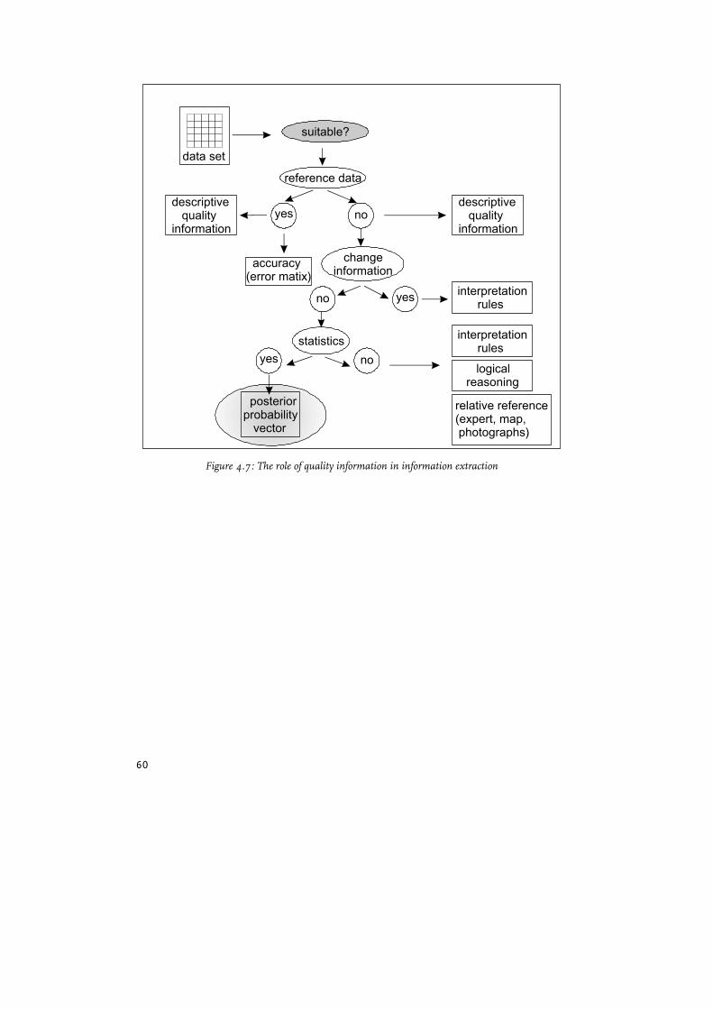
True, probability and other quality information don’t always directly allow for adistinction between “wrong” and “correct” because of their relative meanings.However, quantitative probability information and descriptive meta-information areoften readily available and the problem that needs to be resolved in the followingchapters relates to ways in which this information can be dealt with (see also figure4.7, that will be extended during the following chapters).

60

data set

suitable?

reference data

yes

yes

yes

no

no

no

descriptive quality information

descriptive quality information

accuracy(error matix)

change information

interpretation rules

interpretation rules

statistics

logicalreasoning

relative reference(expert, map, photographs)

posteriorprobability vector

Figure 4.7: The role of quality information in information extraction