4: linear models - the comprehensive r archive network linear models john h maindonald april 3, 2018...

4: Linear Models

John H Maindonald

April 3, 2018

Ideas and issues illustrated by the graphs in this vignette

The graphs shown here relate to issues that arise in the use of the linear modelfitting function lm().

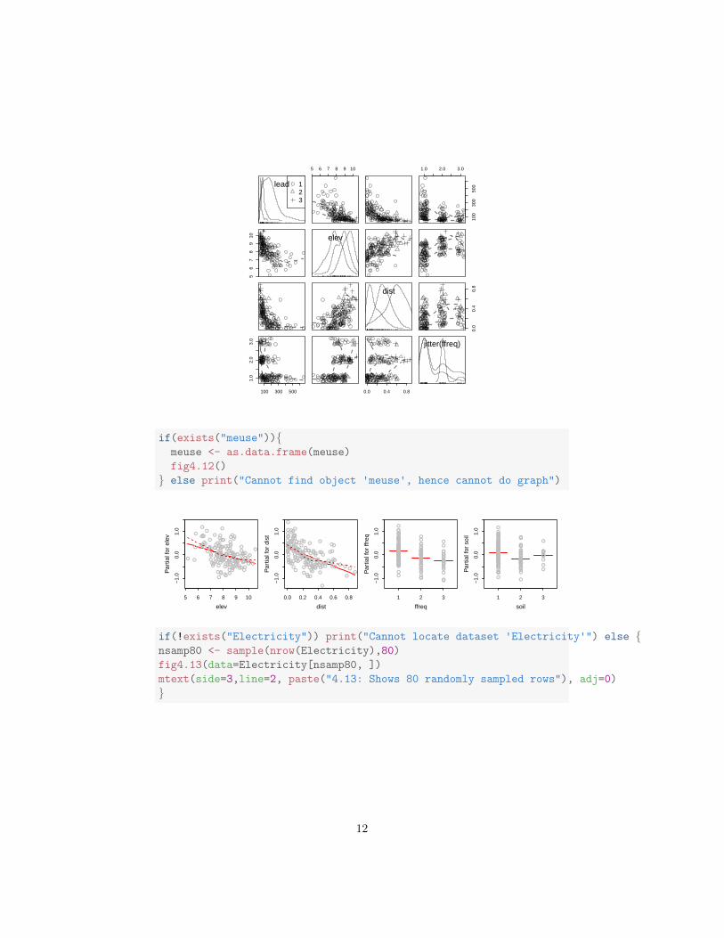
Note: The version of Figure 4.13 that is shown in Section 2 is for a randomsubset of 80 of the 158 rows of the dataset Electricity.

1 Code for Functions that Plot the Figures

fig4.1 <-

function (){size10 <- list(fontsize=list(text=8, points=6))

print(round(cor(nihills), 2))

splom(nihills, par.settings=size10)

}

fig4.2 <-

function ()

{size10 <- list(fontsize=list(text=10, points=6))

lognihills <- log(nihills[,1:4])

names(lognihills) <- c("ldist", "lclim", "ltim", "ltimf")

print(round(cor(lognihills), 2))

vnam <- paste("log(", names(nihills)[1:4], ")", sep="")

splom(lognihills, pscales=0, varnames=vnam, par.settings=size10)

}

fig4.3 <-

function (obj=lognigrad.lm, mfrow=c(1,2))

{

1

objtxt <- deparse(substitute(obj))

nocando <- "Cannot do graph,"

if(!exists(objtxt))return(paste(nocando, "no obj =", objtxt))

opar <- par(mfrow=mfrow)

termplot(obj, col.term="gray", partial=TRUE,

col.res="black", smooth=panel.smooth)

par(opar)

}

fig4.4 <-

function (obj=lognigrad.lm, mfrow=c(1,4)){objtxt <- deparse(substitute(obj))



opar <- par(mfrow=mfrow, pty="s",

mgp=c(2.25,.5,0), mar=c(3.6,3.6,2.1,0.6))

plot(obj, cex.lab=1.4)

par(opar)

}

fig4.5 <-

function (obj=lognigrad.lm, mfrow=c(1,4), nsim=10){opar <- par(mfrow=mfrow, mgp=c(2.25,.5,0), pty="s",

mar=c(3.6,3.6, 2.1, 0.6))

objtxt <- deparse(substitute(obj))



y <- simulate(obj, nsim=nsim)

## Look only at the first simulation

lognisim1.lm <- lm(y[, 1] ~ ldist + lgradient, data=lognihills)

plot(lognisim1.lm, cex.lab=1.1, cex.caption=0.75)

par(opar)

invisible(y)

}

fig4.6 <-

function (obj=lognigrad.lm2)

{objtxt <- deparse(substitute(obj))



opar <- par(mfrow=c(1,4), mgp=c(2.25,.5,0), pty="s",

2

mar=c(3.6,3.6, 2.1, 0.6))

plot(obj, cex.lab=1.1, cex.caption=0.8)

par(opar)

}

fig4.7 <-

function (obj=lognigrad.lm)

{## The following generates a matrix of 23 rows (observations)

## by 1000 sets of simulated responses

simlogniY <- simulate(obj, nsim=1000)

## Extract the QR decomposition of the model matrix

qr <- obj$qr

## For each column of simlogniY, calculate regression coefficients

bmat <- qr.coef(qr, simlogniY)

bDF <- as.data.frame(t(bmat))

names(bDF) <- c("Intercept", "coef_logdist", "coef_lgradient")

gph <- densityplot(~Intercept+coef_logdist+coef_lgradient, data=bDF,

outer=TRUE, scales="free", plot.points=NA,

panel=function(x, ...){panel.densityplot(x, ...)

ci <- quantile(x, c(.025, .975))

panel.abline(v=ci, col="gray")

})

gph

}

fig4.8 <-

function (plotit=TRUE)

{with(DAAG::rice, interaction.plot(x.factor=fert,

trace.factor=variety,

ShootDryMass,

cex.lab=1.2, xpd=TRUE))

}

fig4.9 <-

function (plotit=TRUE)

{## Panel A

gph <- xyplot(tempDiff ~ vapPress, groups=CO2level,

3

data = DAAG::leaftemp,

ylab="", aspect=1,

cex.main=0.75,

par.settings=simpleTheme(pch=c(2,1,6), cex=0.85,

lty=1:3))

hat1 <- predict(lm(tempDiff ~ vapPress, data = leaftemp))

hat2 <- predict(lm(tempDiff ~ vapPress + CO2level, data = leaftemp))

hat3 <- predict(lm(tempDiff ~ vapPress * CO2level, data = leaftemp))

hat123 <- data.frame(hat1=hat1, hat2=hat2, hat3=hat3)

gph1 <- gph+latticeExtra::layer(panel.xyplot(x, hat1, type="l",

col.line=1, ...),

data=hat123)

## Panel B

gph2 <- gph+latticeExtra::layer(panel.xyplot(x, hat2, type="l", ...),

data=hat123)

## Panel C

gph3 <- gph+latticeExtra::layer(panel.xyplot(x, hat3, type="l", ...),

data=hat123)

maintxt <- c(as.call(~ vapPress),

as.call(~ vapPress + CO2level),

as.call(~ vapPress*CO2level))

gph1 <- update(gph1, main=deparse(maintxt[[1]]), ylab="tempDiff",

auto.key=list(text=c("low","med","high"),

between=1, between.columns=2,

columns=3))

gph2 <- update(gph2, main=deparse(maintxt[[2]]),



columns=3))

gph3 <- update(gph3, main=deparse(maintxt[[3]]),



columns=3))

if(plotit){print(gph1, position=c(0,0,.36,1))

print(gph2, position=c(0.34,0,.68,1), newpage=FALSE)

print(gph3, position=c(0.66,0,1,1), newpage=FALSE)

}invisible(list(gph1, gph2, gph3))

}

fig4.10 <-

function ()

{

4

coordinates(meuse) <- ~ x + y

gph <- sp::bubble(meuse, "lead", pch=1, maxsize=2,

main = list("Lead(ppm)", fontface="plain", cex=1.35),

key.entries = 100 * 2^(0:4), col=c(2,4),

scales=list(axes=TRUE, tck=0.4))

add <- latticeExtra::layer(panel.lines(meuse.riv[,1], meuse.riv[,2],

col="gray"))

gph+add

}

fig4.11 <-

function (dset=meuse)

{opar <- par(cex=1.25, mar=rep(1.5,4))

if(!requireNamespace("car"))

return("Function 'car::spm' is unavailable")

if(packageVersion('car') < '3.0.0'){spm(~ lead+elev+dist+jitter(unclass(ffreq)) | soil,

col=adjustcolor(rep("black",3), alpha.f=0.5),

var.labels=c("lead","elev","dist","jitter(ffreq)"),

data=dset, cex.labels=1.5, reg.line=NA)} else

spm(~ lead+elev+dist+jitter(unclass(ffreq)) | soil,

col=adjustcolor(rep("black",3), alpha.f=0.5),

var.labels=c("lead","elev","dist","jitter(ffreq)"),

data=dset, cex.labels=1.5, regLine=FALSE)

par(opar)

}

fig4.12 <-

function (dset=meuse)

{dset$ffreq <- factor(dset$ffreq)

dset$soil <- factor(dset$soil)

meuse.lm <- lm(log(lead) ~ elev + dist + ffreq + soil, data=meuse)

opar <- par(mfrow=c(1,4), mar=c(3.1,3.1,2.6,0.6))

termplot(meuse.lm, partial=TRUE, smooth=panel.smooth)

par(opar)

}

fig4.13 <-

function (data)

{

5

if(packageVersion('car') < '3.0.0'){spm(data, smooth=TRUE, reg.line=NA, cex.labels=1.5,

col=adjustcolor(rep("black",3), alpha.f=0.4))} else

spm(data, smooth=TRUE, regLine=FALSE, cex.labels=1.5,

col=adjustcolor(rep("black",3), alpha.f=0.4))

}

fig4.14 <-

function (data=log(Electricity[,1:2]))

{varlabs = c("log(cost)", "log(q)")

if(!requireNamespace("Ecdat"))return(msg)

if(packageVersion('car') < '3.0.0'){spm(data[,1:2], var.labels=varlabs, smooth=TRUE, reg.line=NA,

col=adjustcolor(rep("black",3), alpha.f=0.5))} else

spm(data[,1:2], var.labels=varlabs, smooth=TRUE, regLine=FALSE,

col=adjustcolor(rep("black",3), alpha.f=0.5))

}

fig4.15 <-

function (obj=elec.lm, mfrow=c(2,4))

{objtxt <- deparse(substitute(obj))



opar <- par(mfrow=mfrow, mar=c(3.1,3.1,1.6,0.6), mgp=c(2,0.5,0))

termplot(obj, partial=T, smooth=panel.smooth)

par(opar)

}

fig4.16 <-

function (obj=elec2xx.lm, mfrow=c(1,4)){objtxt <- deparse(substitute(obj))



opar <- par(mfrow=mfrow, mgp=c(2.25,.5,0), pty="s",

mar=c(3.6,3.6, 2.1, 0.6))

plot(obj, cex.lab=1.1, cex.caption=0.75)

par(opar)

}

6

fig4.17 <-

function (){set.seed(37) # Use to reproduce graph that is shown

bsnVaryNvar(m=100, nvar=3:50, nvmax=3)

}

2 Show the Figures

pkgs <- c("DAAG","sp","splines","car","leaps","sp","quantreg")

z <- sapply(pkgs, require, character.only=TRUE, warn.conflicts=FALSE)

if(any(!z)){notAvail <- paste(names(z)[!z], collapse=", ")

print(paste("The following packages should be installed:", notAvail))

}

if(!exists("Electricity")){msg <- "Cannot locate 'Electricity' or 'Ecdat::Electricity'"

if(require("Ecdat")) Electricity <- Ecdat::Electricity else

print(msg)

if(require("sp")){data("meuse", package="sp", envir=environment())

} else print("Package 'sp' is not available")

}

fig4.1()

dist climb time timef

dist 1.00 0.91 0.97 0.95

climb 0.91 1.00 0.97 0.96

time 0.97 0.97 1.00 1.00

timef 0.95 0.96 1.00 1.00

7

Scatter Plot Matrix

dist10

15 10 15

5

10

5 10●

●●

●●●●●●

●

●●●●●

●

●

●

●

●●

●●

●

●●

●●●●●●

●

●●●●●

●

●

●

●

●●

●●

●

●●

●●●●●●

●

●●●●●

●

●

●

●

●●

●●

●● ●

●

●●●●●

●

●●●

●●

● ●●

●

●●●●

climb6000

80006000

2000

4000

2000●

●●

●

●●●●●

●

●●

●●●

● ●●

●

●●●● ●

●●

●

●●●●●

●

●●

●●●

● ●●

●

●●●●

●●

●●

●●●●●

●

●●●●●●

●

●

●

●●●● ●

●●

●

●●●●●

●

●●●●●●

●

●

●

●●●●

time

3

4

3 4

1

2

1 2 ●●●

●

●●●●●

●

●●●●●●

●

●

●

●●●●

●● ●

●●●●●●

●

●●●●●

●

●

●

●

●●●● ●

●●●

●●●●●

●

●●●●●

●

●

●

●

●●●●

●●●

●●●●●●

●

●●●●●

●

●

●

●

●●●●

timef4

5

6

4 5 6

1

2

3

1 2 3

fig4.2()

ldist lclim ltim ltimf

ldist 1.00 0.78 0.95 0.93

lclim 0.78 1.00 0.92 0.92

ltim 0.95 0.92 1.00 0.99

ltimf 0.93 0.92 0.99 1.00

Scatter Plot Matrix

log(dist) ●

●

●●

●●●

●●

●

● ●●●

●●

●

●

●

●

●

●●

●

●

●●

●●●

●●

●

● ●●●●

●

●

●

●

●

●

●●

●

●

●●

●●●

●●

●

● ●●●●

●

●

●

●

●

●

●●

●

● ●

●

●●

●●●

●

●

●●

●●

● ●●

●

●●

● ●

log(climb)●

● ●

●

●●

●●●

●

●

●●

●●

● ●●

●

●●

●●●

● ●

●

●●

●●●

●

●

●●

●●

● ●●

●

●●

●●

●

●

●

●

●●●

●●

●

●●

●●

●

●

●

●

●

●●

● ●●

●

●

●

●●●●●

●

●●

●●

●

●

●

●

●

●●

●●

log(time)●

●

●

●

●●●

●●

●

●●

●●●

●

●

●

●

●●

●●

●

●

●●

●●●●●

●

●

●●● ●

●

●

●

●

●●

●● ●

●

●●

●●●●●

●

●

●● ●●

●

●

●

●

●●

●● ●

●

●●

●●●●●

●

●

●●●●

●

●

●

●

●●

●●

log(timef)

8

nihills[,"gradient"] <- with(nihills, climb/dist)

lognihills <- log(nihills)

names(lognihills) <- paste("l", names(nihills), sep="")

lognigrad.lm <- lm(ltime ~ ldist + lgradient, data=lognihills)

lognigrad.lm2 <- lm(ltime ~ poly(ldist, 2, raw=TRUE) + lgradient,

data=lognihills)

fig4.3()

1.0 1.5 2.0 2.5 3.0

−0.

50.

00.

51.

01.

5

ldist

Par

tial f

or ld

ist

●

●

● ●

●●

●

●●

●

●●

●

●

●

●

●

●

●

●

●

●

●

5.4 5.8 6.2

−0.

50.

00.

51.

01.

5

lgradient

Par

tial f

or lg

radi

ent

● ●●

●

●●

●

●

●

●

●

●● ●

●

●

●

●●

●●

●●

fig4.4()

−1.0 0.0 1.0

−0.

20−

0.05

0.10

Fitted values

Res

idua

ls

●●

●

●

●●

●

●

●

●

●●

●

●

●

●

●●

●

●

●

●

●

Residuals vs Fitted

Meelbeg Meelmore

Hen & Cock

Donard Forest

●●

●

●

●●

●

●

●

●

●●

●

●

●

●

●●

●

●

●

●●

−2 −1 0 1 2

−2

−1

01

2

Theoretical Quantiles

Sta

ndar

dize

d re

sidu

als Normal Q−Q

Meelbeg Meelmore

Hen & CockSeven Sevens

−1.0 0.0 1.0

0.0

0.5

1.0

1.5

Fitted values

Sta

ndar

dize

d re

sidu

als

●●

●●

●

●

●

●

●

●●

●

●

●

●

●

●●

●

●●

●

●

Scale−LocationMeelbeg Meelmore

Hen & CockSeven Sevens

0.0 0.1 0.2 0.3 0.4

−2

−1

01

2

Leverage

Sta

ndar

dize

d re

sidu

als

●●

●

●●

●

●

●

●

●

●●

●

●

●

●

● ●

●

●

●

●●

Cook's distance10.5

0.51

Residuals vs Leverage

Seven SevensHen & Cock

Meelbeg Meelmore

fig4.5()

−1.0 0.0 1.0

−0.

150.

000.

10

Fitted values

Res

idua

ls

●

●

●

●

●●

●

●

●

●

●

●

●

●●

●

●

●

●

●

●●

●

Residuals vs Fitted

Slieve DonardAnnalong Horseshoe

Donard & Commedagh

●

●

●

●

●●

●

●

●

●

●

●

●

●●

●

●

●

●

●

●

●

●

−2 −1 0 1 2

−1

01

2


Sta

ndar

dize

d re

sidu

als Normal Q−Q

Seven Sevens

Annalong HorseshoeSlieve Donard

−1.0 0.0 1.0

0.0

0.4

0.8

1.2

Fitted values

Sta

ndar

dize

d re

sidu

als

●

●

●

●

●●

●

●

●

●

●

●

●

●

●

●

●

●

●

●

●

●

●

Scale−LocationSeven SevensAnnalong HorseshoeSlieve Donard

0.0 0.1 0.2 0.3 0.4

−2

−1

01

2

Leverage

Sta

ndar

dize

d re

sidu

als

●

●

●

●

● ●

●

●

●

●

●

●

●

●●

●

●

●

●

●

●●

●

Cook's distance10.5

0.5

1


Seven Sevens

Annalong HorseshoeSlieve Bearnagh

9

fig4.6()

−1.0 0.0 1.0

−0.

20−

0.05

0.05

Fitted values

Res

idua

ls

●●

●

●●●

●

●

●

●

●

●

●

●

●

●

●●

●

●●

●●

Residuals vs Fitted

Meelbeg Meelmore

Glenariff Mountain Slieve Gallion

●●

●

●●●

●

●

●

●

●

●

●

●

●

●

●●

●

●●

●●

−2 −1 0 1 2

−2

−1

01

2

Theoretical QuantilesS

tand

ardi

zed

resi

dual

s Normal Q−Q

Meelbeg Meelmore

Glenariff MountainSlieve Donard

−1.0 0.0 1.0

0.0

0.5

1.0

1.5

Fitted values

Sta

ndar

dize

d re

sidu

als

●

●

●

●●●

●

●

●

●●

●

●

●

●●

●

●

●●

●

●

●

Scale−LocationMeelbeg Meelmore

Glenariff MountainSlieve Donard

0.0 0.2 0.4 0.6

−3

−2

−1

01

2

Leverage

Sta

ndar

dize

d re

sidu

als

●●

●

●●●

●

●

●

●

●

●

●

●

●

●

●●

●

●●

●●

Cook's distance

10.5

0.51


Hen & Cock

Meelbeg Meelmore

Seven Sevens

fig4.7()

Intercept + coef_logdist + coef_lgradient

Den

sity

0.0

0.5

1.0

−6.0 −5.5 −5.0 −4.5 −4.0

Intercept

02

46

810

12

1.05 1.15 1.25

coef_logdist

02

46

80.3 0.4 0.5 0.6

coef_lgradient

if (require("DAAG")) fig4.8()

2040

6080

100

fert

mea

n of

Sho

otD

ryM

ass

F10 NH4Cl NH4NO3

variety

wtANU843

if (require("DAAG")) fig4.9()

10

~vapPress

vapPress

tem

pDiff

0

1

2

3

1.5 2.0 2.5

●

●

●

●

●

●●

●

●●

●

●

●

●

●

●

●

●

●

●●

low med high●

~vapPress + CO2level

vapPress

0

1

2

3

1.5 2.0 2.5

●

●

●

●

●

●●

●

●●

●

●

●

●

●

●

●

●

●

●●

low med high●

~vapPress * CO2level

vapPress

0

1

2

3

1.5 2.0 2.5

●

●

●

●

●

●●

●

●●

●

●

●

●

●

●

●

●

●

●●

low med high●

if(require("sp")) {data("meuse.riv", package="sp", envir = environment())

data("meuse", package="sp", envir = environment())

} else

print("Cannot find package 'sp' or required data, cannot do graph")

if(exists("meuse")){meuse <- as.data.frame(meuse)

fig4.11()

} else print("Cannot find object 'meuse', hence cannot do graph")

11

123

lead

5 6 7 8 9 10 1.0 2.0 3.0

100

300

500

56

78

910 elev

dist

0.0

0.4

0.8

100 300 500

1.0

2.0

3.0

0.0 0.4 0.8

jitter(ffreq)

if(exists("meuse")){meuse <- as.data.frame(meuse)

fig4.12()

} else print("Cannot find object 'meuse', hence cannot do graph")

5 6 7 8 9 10

−1.

00.

01.

0

elev

Par

tial f

or e

lev

●●

●●

●

●

●

●●●●

●

●

●

●

●

●●

●

●

●

●●

●●●●

●●●

●

●●

●●●

●●●

●

●

●

●●

●●

●

● ●

●

●

●

●

●

●

●

●●

●

●

●

●●●

●●

●

●

●

● ●●

●●●●

●

●

●●

●

●

●●

●

●

●

●

●●

● ●●

●

●●

●

●●●

●

●

●

●

●●●●●

●

●

● ●●

●

● ●

●

●●

●●

●●

● ●●●

●●

●

●

●

●

●●●●

●

●

●

●●

●

●●

●

●

●●

●

●

●

●

●

0.0 0.2 0.4 0.6 0.8

−1.

00.

01.

0

dist

Par

tial f

or d

ist

●

●

●

● ●

●●●

●●●●

●

●

●

●

●●

●

● ●

●● ●

●●●●

●

●●

●● ●●●

●●●

●

●

●

● ●

●

●●

● ●

●

●

●

●

●

●

●

●●

●

●

●

●●●

●

●

●

●

●

● ●

●

●●●

●●

●

●●

●

●

●

●●

●

●

●●

● ●

●●

●

● ●

●●●

●●

●

●

●●

●●

●

●

●

●

●●

●

●

●●

●

●●

●●

●

●

●

●● ●

●●

●

●

●●

●●

●

●

●

●

●

●●

●

●●

●

●

●

●

●

●

●

●

●

−1.

00.

01.

0

ffreq

Par

tial f

or ff

req

1 2 3

●

●●●●

●

●

●●●●

●

●●

●

●

●●

●

●●

●●

●●●

●●

●●●

●●●●●

●●●

●

●

●

●●

●●●

●●

●

●

●

●

●

●

●

●●

●

●

●

●●●

●

●

●

●

●

●●●●●●

●●●

●●

●

●

●

●

●

●

●

●

●●●●●

●

●●●

●●●

●

●

●●●●●●●

●

●

●●●

●

●

●

●

●●

●●

●●

●●●●●●

●

●

●

●

●●●●

●●

●

●●

●

●

●

●

●

●●

●

●

●

●

●

−1.

00.

01.

0

soil

Par

tial f

or s

oil

1 2 3

●

●●

●●

●

●●●

●●●

●●

●

●

●●

●

●●

●● ●●●

●●

●●●

●●●●●

●●●

●

●

●

●●

●●●

●●

●

●●

●

●

●

●

●●

●

●

●

●●●

●

●

●

●

●

●●●●●●

●●●

●●

●

●

●

●●

●

●

●

●●●●●

●

●●●

●●●

●

●

● ●●●●●●

●

●

●●●

●

●

●

●

●●●●

●●

●

●●●

●●

●

●●

●

●●

●●

●●

●

●●

●

●

●

●

●

●●

●

●

●

●

●

if(!exists("Electricity")) print("Cannot locate dataset 'Electricity'") else {nsamp80 <- sample(nrow(Electricity),80)

fig4.13(data=Electricity[nsamp80, ])

mtext(side=3,line=2, paste("4.13: Shows 80 randomly sampled rows"), adj=0)

}

12

cost

0 80000 0.05 0.20 0.15 0.35 0.4 0.7

040

0

080

000 q

pl

6000

1000

0

0.05

0.20 sl

pk

3060

90

0.15

0.35 sk

pf

1030

50

0 400

0.4

0.7

6000 10000 30 60 90 10 30 50

sf

4.13: Shows 80 randomly sampled rows

if(exists("Electricity")){elec.lm <- lm(log(cost) ~ log(q)+pl+sl+pk+sk+pf+sf, data=Electricity)

elec2xx.lm <- lm(log(cost) ~ log(q) * (pl + sl) + pf, data = Electricity)

}

if(exists("Electricity"))fig4.14() else

print("Cannot locate dataset 'Electricity'; graph unavailable")

13

log(cost)

2 4 6 8 10 12

−2

02

46

−2 0 2 4 6

24

68

1012

log(q)



0 40000 80000 120000

−6

−4

−2

02

q

Par

tial f

or lo

g(q)

●

●

●

●

●●

●

●

●

●

●

●

●

●

●●●●

●

●

●

●●●

●●●●●●

●●●●●

●

●

●

●●●●

●●●●●

●●●●●●●

●●●●

●

●●●

●●●●●●

●●●●

●●

●

●●

●●

●●

●●●●

●

●●●●●

●●●●●●●●●●●

●●

●

●

●

●

●●●

●●

●

●

●●

●

●

●

●

●●●

●

●●●●

●

●

●●

●

●●●●●●

●

●

●●●

●●●●

●

●

●

●

●●●

●

●

6000 10000

−6

−4

−2

02

pl

Par

tial f

or p

l

●

●● ●●● ●

● ●

●●● ●●● ●●●● ●●● ● ●● ●●●● ●● ●

●●

●● ●● ●●●●● ●● ●●●● ●●●● ● ●●●●● ● ●● ●● ●● ●● ●● ● ●●●●● ● ●●●●● ● ●●

●

●●

●●●● ●● ●●● ● ●●●●● ● ●●●●● ●●● ●● ●

●● ● ●●●

●●●●● ●●● ●

● ●●●

●● ● ● ●●●●● ●●● ●●●●

●● ●●

●● ●●

0.05 0.15 0.25

−6

−4

−2

02

sl

Par

tial f

or s

l ●

●●●

●●●●●

●● ●●● ●

●● ●●● ●● ●

●● ●●● ●●●●

●●

●● ●● ●●●●●●

●●●● ●●●● ●● ●●●●● ●●

●● ●●● ●● ●● ●●● ●● ●● ●● ●●

● ● ●●●

● ●●●●● ●●●●

●●●●

● ●●●● ●● ●● ●●●● ●●●●●● ●●

● ●●●● ●● ●● ●●● ●●●●● ● ●● ●● ●● ●●●●●

●

● ●●

●●● ●

30 40 50 60 70 80 90

−6

−4

−2

02

pk

Par

tial f

or p

k

●

●●● ●● ●●●

●●●● ●●

●●●● ●● ●●● ●●● ● ●●● ●●

●● ●●● ●●●● ●● ● ●● ●● ●●●● ●●● ●● ●●●●● ● ● ●● ●●●●● ●●● ●● ●● ●● ●●● ●

●

●● ● ●

●●●● ●●●●●● ●●●●●●● ● ●● ●●● ●●

●●● ●●●●● ●●

●● ●● ●●

●●●●● ●●●● ● ● ●●● ●● ●●●

●●●

●● ●●●

0.1 0.2 0.3 0.4

−6

−4

−2

02

sk

Par

tial f

or s

k ●

●●●● ●●

●●

●● ●● ●●● ●●●●●●●● ● ●● ● ●●●●●

●●●● ●● ●● ●● ● ●●● ●●●●● ●●● ●●● ●●● ●● ● ●● ● ●●● ●●●●●●● ●●●●● ●● ●

●●

●●●

●● ●●●●● ●● ●● ●●●●

●●● ● ● ●● ●●●●

●● ● ●●● ●●●● ●●●

●●

● ●●

● ●● ●●●●● ●●●● ●●● ●●●●

●●● ● ●

10 20 30 40 50

−6

−4

−2

02

pf

Par

tial f

or p

f

●

●

●● ●●●●

●

●

●●●

●●●●

● ● ● ●●

●●●● ● ●●

●●●●

●

● ● ●●●

● ●●●

●●

●●●●●

●● ● ●●●● ●●

●●

●● ●●●●

●●●●

●●●●

●● ●● ●●●● ● ●

●● ●●●

●

●●●● ●

● ●●●●

● ●●●

● ● ●●●●●● ●● ●●

● ●●●

●●●●

●●● ●● ●

●● ●● ●●●●● ●● ●● ● ●● ●● ●

●●●

●● ●●●

0.3 0.5 0.7

−6

−4

−2

02

sf

Par

tial f

or s

f ●

● ●●●●●

● ●

●●● ●●●

● ●● ●●● ●●● ●● ●●● ● ●●●

●● ●●●●● ●● ●●● ●●●● ●●●● ●●● ● ●●●●● ●●● ●●●● ●● ●●●●● ●● ●●● ●●●●●

●● ● ●

● ●● ● ●●●●●● ●● ● ●●

● ●●●● ● ●●●●●

● ●●●●●●●●

●● ●●●●

●●●● ●●●● ● ●●● ● ●●●●●●

●●●

●● ●●●



−2 0 2 4 6

−0.

40.

00.

4

Fitted values

Res

idua

ls

●

●

●●

●●

●●

●

●

●●

●

●

●

●

●

●

●●●

●

●●●●

●

●●●●

●

●

●

●

●●

●●●

●

●

●

●●●

●●●●●●

●●

●●●●

●●●

● ●

●●

●

●●

●●

●●●●

●

●

●●

●●

●●

●●

●

● ●

●●

●

● ●

●●●

●

●●●

●

●●

●●

●

●●● ●

●●

●●

●

●

●

●

●●

●

●●●

●●

●●

●

●

●

●

●●

●

●●

●

●●

●

●●●

●●

●●●●

●

●

●

●●

●

●

●

●

Residuals vs Fitted

151

3387

●

●

●●

●●

●●

●

●

●●

●

●

●

●

●

●

●●●

●

●●●●

●

●●●●

●

●

●

●

●●

●●●

●

●

●

●●

●

●●●●

●●

●●

●

●●●

●● ●

●●

●●

●

●●

●●

●●●●

●

●

●●

●●

●

●●●

●

●●

●●

●

●●

●●●

●

●●●

●

●

●

●●

●

●●●●

●●

●●

●

●

●

●

●●

●

●●

●

●●

●●

●

●

●

●

●●

●

●●

●

●●

●

●●●

●●

●●●●

●

●

●

●●

●

●

●

●

−2 0 1 2

−2

02

4


Sta

ndar

dize

d re

sidu

als Normal Q−Q

151

3387

−2 0 2 4 6

0.0

0.5

1.0

1.5

2.0

Fitted values

Sta

ndar

dize

d re

sidu

als

●●

●

●

●

●

●

●

●

●

●●

●

●

●

●

●

●

●

●

●

●

●

●

●●

●

●●● ●

●

●

●

●

●

●

●

●●

●

●●●

●

●

●●

●●

●

●

●

●

●

●

●●

●

●●

●

●

●

●

●

●

●●

●

●●

●

●

●

●

●

●

●

●

●

●

●●

●

● ●

●

●

●●

●

●

●

●

●

●

●

●

●

●

●

●

●

●

●

●●

●

●●

●

●

●

●

●

●●

● ●

●●●

●●

●

●

●●

●

●

●

●

●

●●

●

●

●

●

●●

●

●

●

●

●●●

●

●

●●

●●

●

●●

Scale−Location151

3387

0.00 0.10 0.20 0.30

−2

02

4

Leverage

Sta

ndar

dize

d re

sidu

als

●

●

●●

●●

●●

●

●

● ●

●

●

●

●

●

●

●●●

●

● ●●●

●

● ●●●

●

●

●

●

●●

●●●

●

●

●

●●●

●●●●●●

●●

●●●●

●● ●

●●

●●

●

●●

●●

●●●●

●

●

●●

●●

●●

● ●

●

●●

●●

●

●●

●●●

●

●●●

●

●●

●●

●●

● ●●●

●●

●

●

●

●

●

●●

●

●●●

●●

●●

●

●

●

●

●●

●

●●

●

●●

●

●●●

●●

●●●●

●

●

●

●●

●

●

●

●

Cook's distance1

0.5

0.5

1


86

151

10

14

if(require(DAAG)) fig4.17()

●

●

●

●

●

●

●

●

●

●●

●

●

●●●

●

●

●●

●●

●

●

●●●

●●

●●●

●●

●●●

●

●●●●

●

●●

●

●

●

●

●

●

●

●

●

●●

●

●

●

●

●

●

●●●

●

●

●

●●

●●●

●

●●

●

●

●

●

●●●

●

●●

●

●

●●●●●

●

●

●

●

●●

●

●

●

●

●

●

●

●

●

●

●●●

●●

●●

●

●

●

●

●

●

●

●

●●●●●

●

●●●●●●

●●

●

●

●●●

●

# of variables from which to select

p−va

lues

for

t−st

atis

tics

0 10 20 30 40 50

0.001

0.01

0.05

0.25

0.5

0.75Select 'best' 3 variables

15

4: linear models - the comprehensive r archive network linear models john h maindonald april 3, 2018...

Documents