4. distributed loads - chulalongkorn...
TRANSCRIPT
1
4. Distributed Loads
2142111 S i 2011/22142111 Statics, 2011/2
© Department of Mechanical Engineering Chulalongkorn UniversityEngineering, Chulalongkorn University
2
Objectives Students must be able to #1Objectives Students must be able to #1
Course ObjectiveI l d di t ib t d l d i t ilib i l Include distributed loads into equilibrium analyses
Chapter Objectives Describe the characteristics and determine the centroids, Describe the characteristics and determine the centroids,
centers of mass and centers of gravity by integration and composite body methods
Apply the Pappus Theorems for surface and volume of Apply the Pappus Theorems for surface and volume of revolution
Describe the characteristics and determine the first moment of f farea, second moment of area and polar moment of inertia by
integration, parallel-axis theorem and perpendicular-axis theorem
2
Determine the resultant of loads (force/couple) with line, area and volume distribution by integration and area/volume analogy
3
Objectives Students must be able to #2Objectives Students must be able to #2
Analyze bodies/structures with distributed loads for unknown loads/reactions by appropriate FBDsloads/reactions by appropriate FBDs
For fluid statics Describe the characteristics and determine hydrostatic and
aerostatic pressures as distributed loads Determine the resultant of fluid statics by integration volume Determine the resultant of fluid statics by integration, volume
analogy and block-of-fluid methods Describe and determine the buoyancy and stability of floating
bodies Analyze bodies/structures with fluid statics for unknown
loads/reactions by appropriate FBDs
3
y pp p
4
Objectives Students must be able to #3Objectives Students must be able to #3
For flexible cablesSt t th ti d t i l d fi iti f fl ibl State the assumptions and geometrical definitions of flexible cables
Appropriately approximate real-life cables into parabolic or pp p y pp pcatenary cables by load distribution
Prove and apply profile, length and tension formula for parabolic & catenary cablesparabolic & catenary cables
Identify and utilize techniques for obtaining numerical solutions of parabolic & catenary cables
4
5
ContentsContents Centroid, Center of Mass and Center of Gravity
Pappus Theorems Pappus Theorems First Moment of Area, Moment of Inertia, Polar Moment of
Inertia Distributed Loads Fluid Statics
Flexible Cables Flexible Cables
5
6
Software HelpsSoftware Helps 3M Software
Maple Computer Center Maple – Computer Center MatLab – Computer Center Mathematica
MapleS l t M l i th ‘St t M ’ Select Maple in the ‘Start Menu’
Type in commands, then ‘Enter’ Use ‘Help Menu’ for command templates Use Help Menu for command templates
6

7
Centers of Gravity High School
Center
Centers of Gravity High School
F
x11x2
x3x4
F
G1 2 3 4x x x x+ + +
7
x 1 2 3 4
4x x x xx + + +
=
8
Centers of Gravity, CGCenter
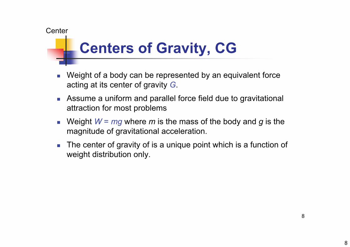
Centers of Gravity, CG Weight of a body can be represented by an equivalent force
acting at its center of gravity G.
Assume a uniform and parallel force field due to gravitational attraction for most problemsattraction for most problems
Weight W = mg where m is the mass of the body and g is the magnitude of gravitational acceleration.
The center of gravity of is a unique point which is a function of weight distribution only.
8
9
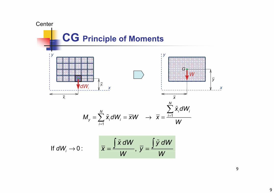
CG Principle of Moments
Center
CG Principle of Moments
N
x dW 1
1
i iNi
y i ii
x dWM x dW xW x
W=
=
= = → =
, x dW y dW
x yW W
= = If 0 :idW →
9
, yW Wi
10
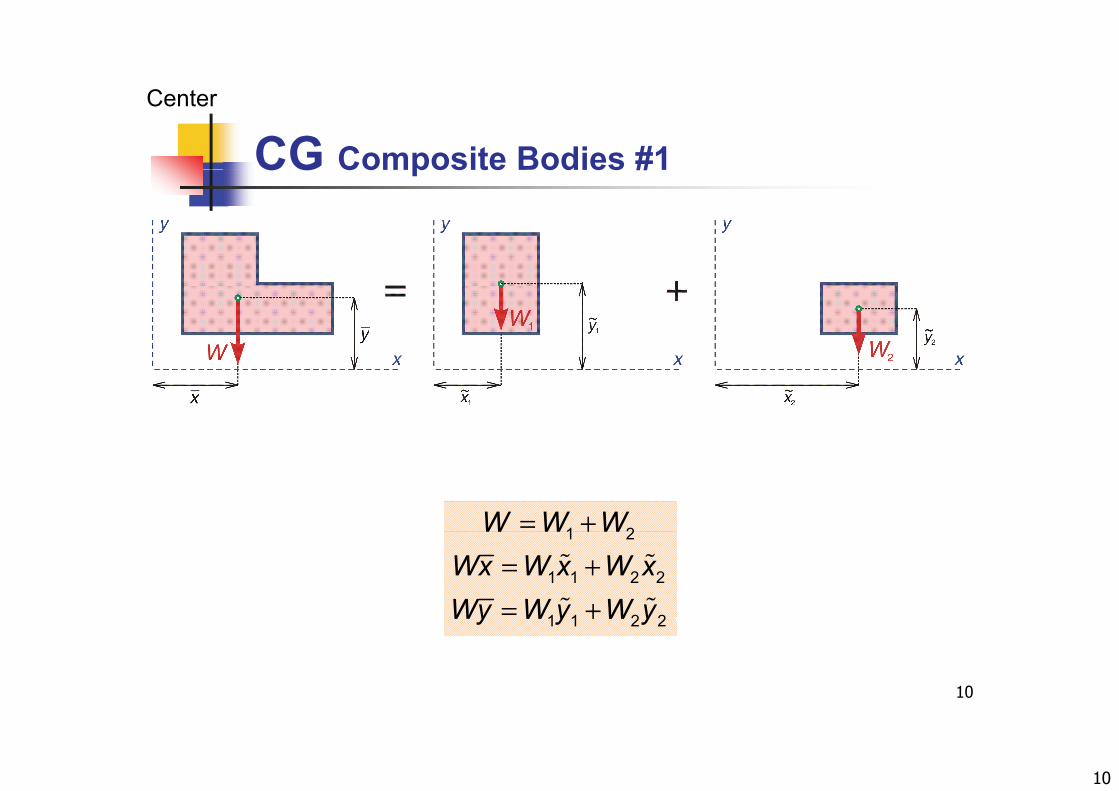
CG Composite Bodies #1
Center
CG Composite Bodies #1
1 2W W W= +1 2
1 1 2 2
1 1 2 2
W W WWx W x W xWy W y W y
+= += +
10
1 1 2 2y y y
11
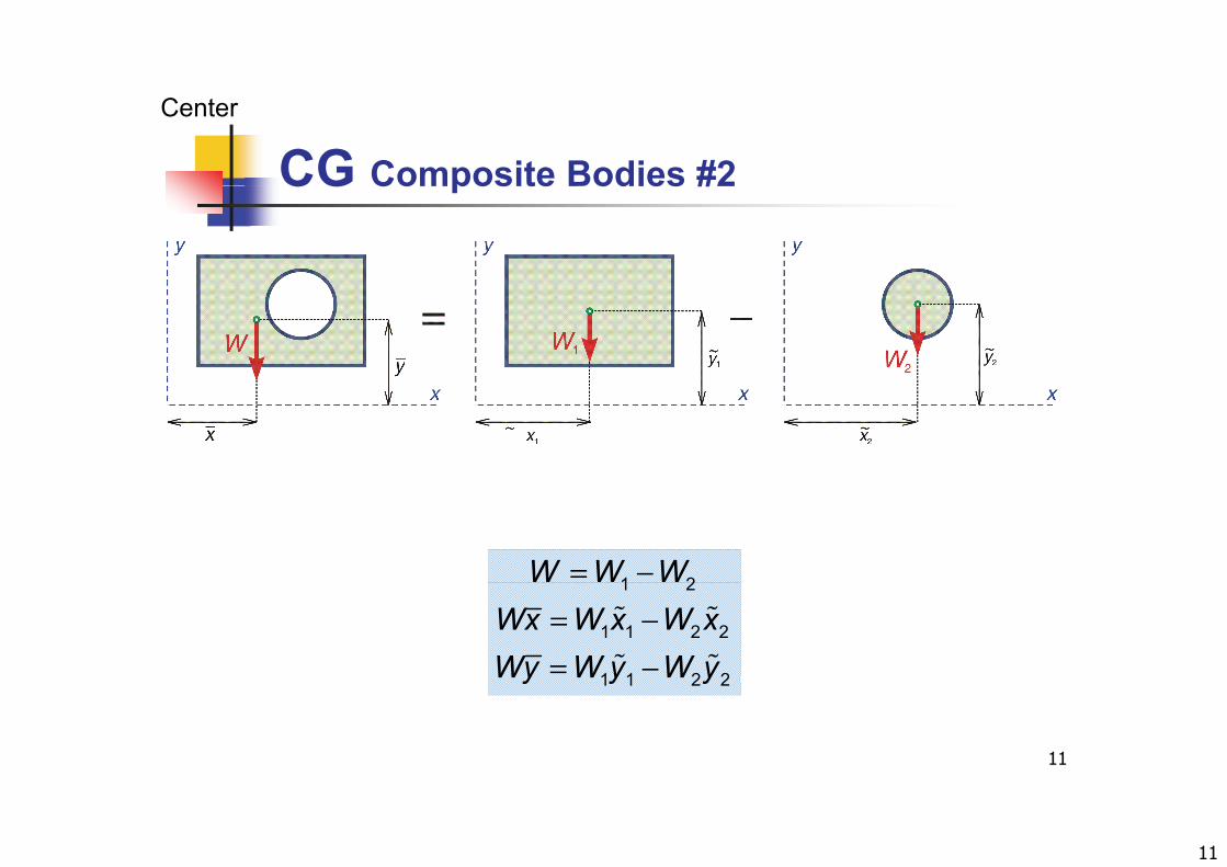
CG Composite Bodies #2
Center
CG Composite Bodies #2
1 2W W W= −1 2
1 1 2 2
1 1 2 2
Wx W x W xWy W y W y
= −= −
11
1 1 2 2y y y
12
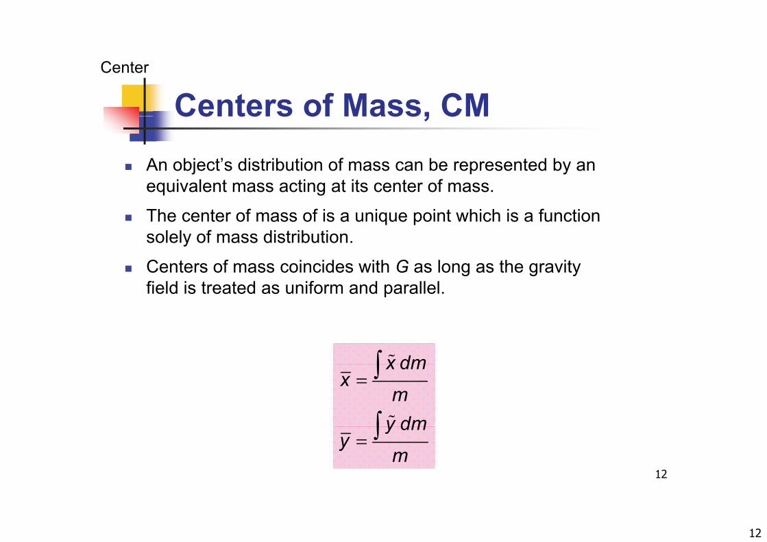
Centers of Mass, CMCenter
An object’s distribution of mass can be represented by an
Centers of Mass, CM
equivalent mass acting at its center of mass.
The center of mass of is a unique point which is a function solely of mass distributionsolely of mass distribution.
Centers of mass coincides with G as long as the gravity field is treated as uniform and parallel.
x dm x dmx
my dm
=
12
y dmy
m=
13
CentroidsCenter
If the density ρ is constant and and gravity field is uniform and parallel G and center of mass coincide with the
Centroids
and parallel, G and center of mass coincide with the centroid of the body.
The centroid C is the geometrical center or the weighted average position of an object.
Locating the centroid by averaging the ‘moments’ of elements of objects about axeselements of objects about axes.
The centroid lies on the axis of symmetry.
Geometry of the body is the only factor that influence theGeometry of the body is the only factor that influence the position of the centroid.
13
14
Centroids Formula
Center
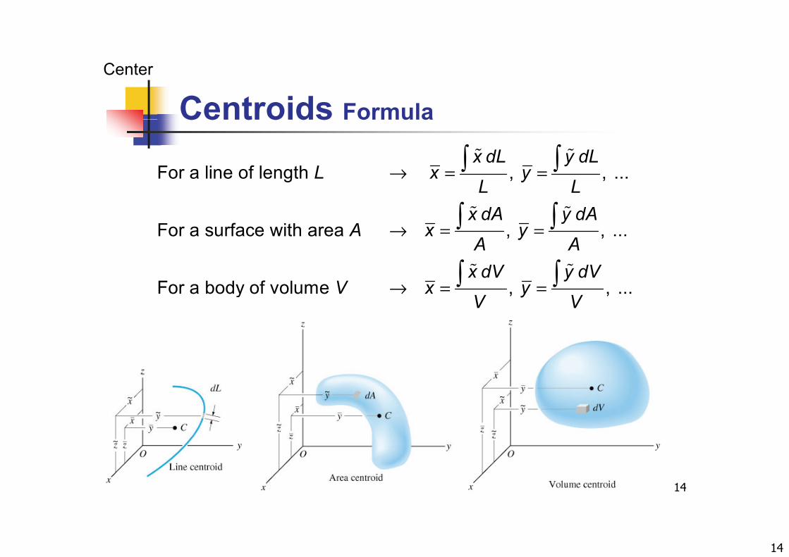
Centroids Formula
For a line of length , , ...x dL y dL
L x yL L
→ = =
For a surface with area , , ...
L Lx dA y dA
A x yA A
→ = =
For a body of volume , , ...
A Ax dV y dV
V x yV V
→ = =
14
15
Centroids Symmetry
Center
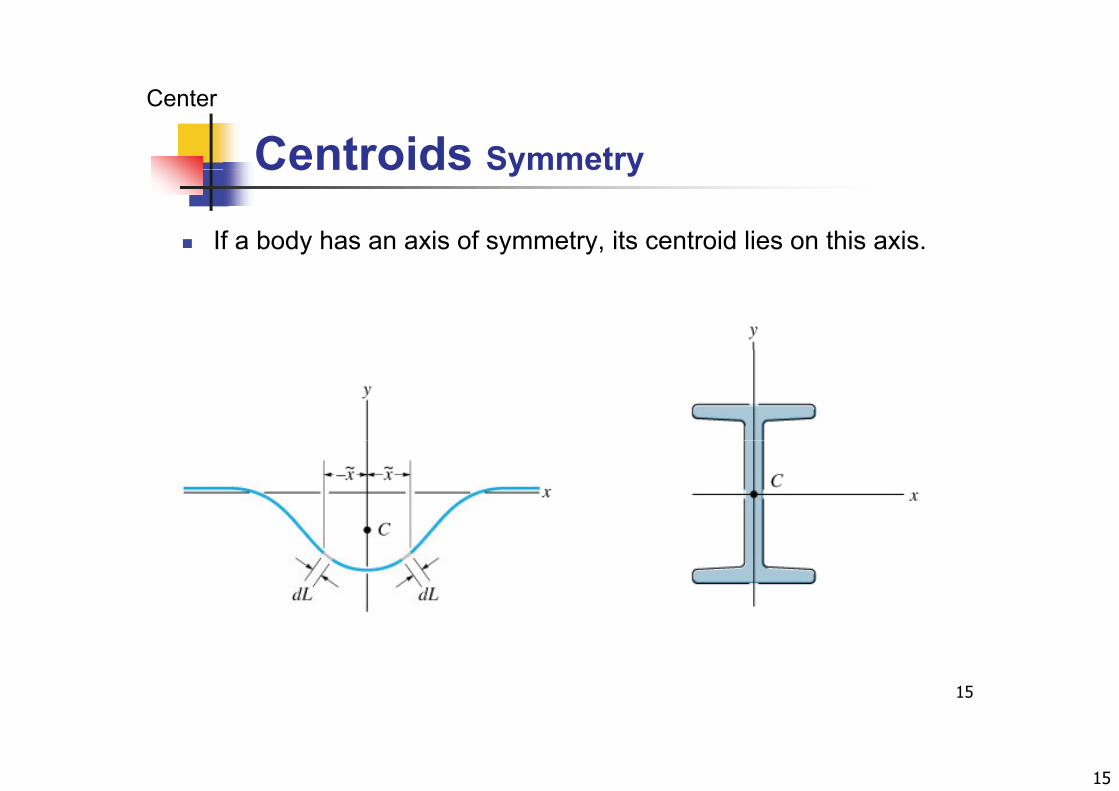
Centroids Symmetry
If a body has an axis of symmetry, its centroid lies on this axis.
15
16
Example Centroids 1 #1
Center
Example Centroids 1 #1
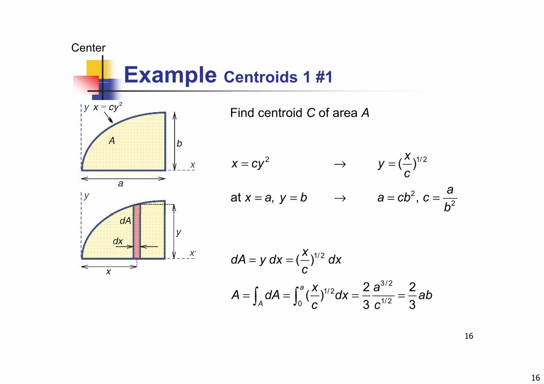
Find centroid C of area A
2 1/ 2 ( )xx cy y= → =
22at , ,
cax a y b a cb cb
= = → = =
1/ 2( )xdA y dx dx 1/ 2
3 / 21/ 2
1/ 20
( )
2 2( )3 3
a
A
dA y dx dxc
x aA dA dx ab
= =
= = = =
16
1/ 20 3 3A c c
17
Example Centroids 1 #2
Center
p
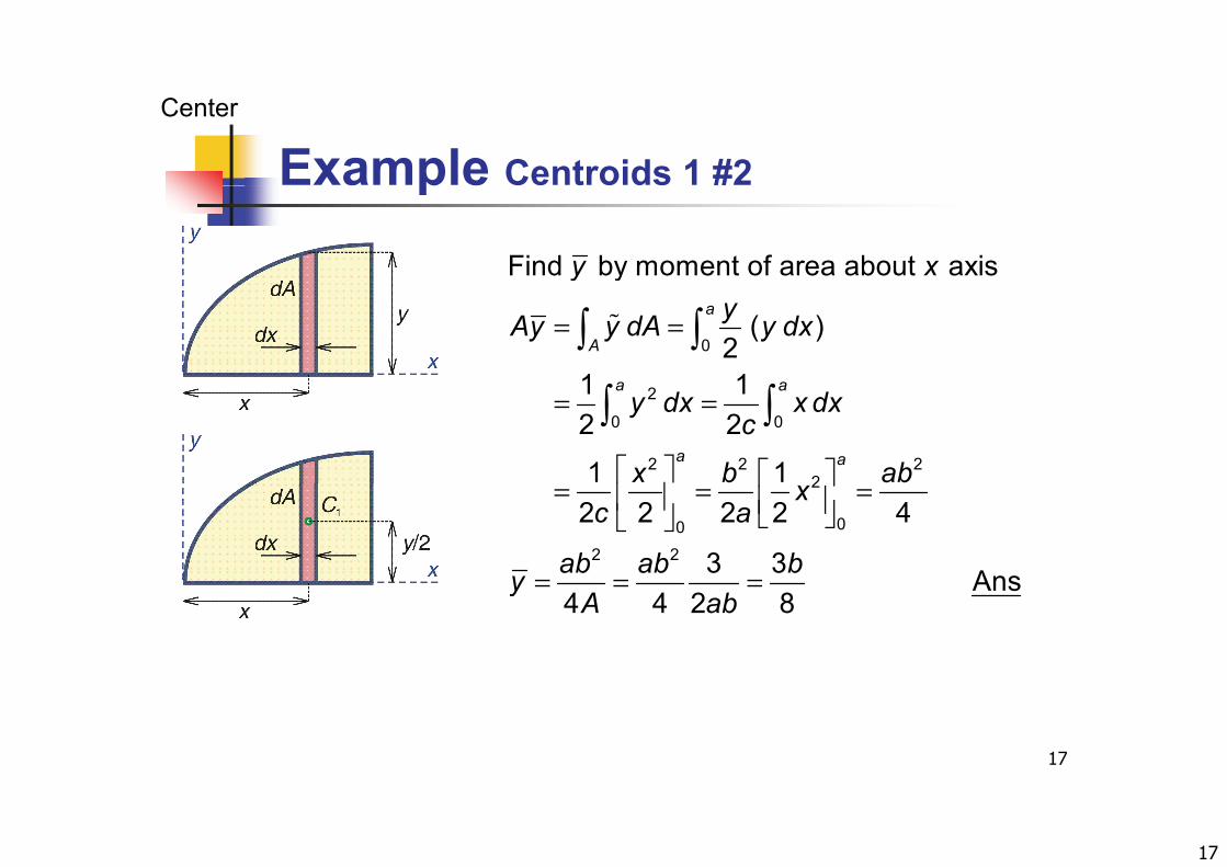
Find by moment of area about axisy x
= =
0
( ) 2
1 1
a
A
a a
yAy y dA y dx
= =
2
0 0
2 2 22
1 12 2
1 1
a a
a a
y dx x dxc
x b abA
Ay
= = =
= = =
2
002 2
2 2 2 2 4
3 3 Ans
xc a
ab ab b
Ay
y = = = Ans4 4 2 8b
yA a
17
18
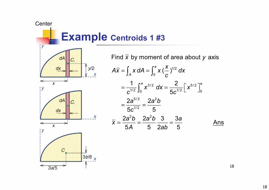
Example Centroids 1 #3
Center
pFind by moment of area about axisx y
= =
1/2
0
3 / 2 5 / 2
( )
1 2
a
A
a a
xAx x dA x dxc
= =
= =
3 / 2 5 / 21/ 2 1/ 2 00
5 / 2 2
1 2 5
2 2
a axAx
A
dx xc ca a bx = =
= = =
1/ 2
2 2
552 2 3 3 Ans5 5 2 5
Ac
a b a b axA ab
x
5 5 2 5A ab
18
19
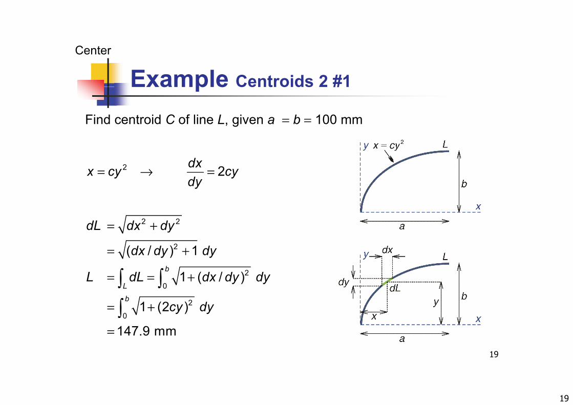
Example Centroids 2 #1
Center
Example Centroids 2 #1
Find centroid C of line L, given a = b = 100 mm
2 2dxx cy cydy
= → =
2 2
dy
dL dx dy= +2
2
( / ) 1
1 ( / )b
dL dx dy
dx dy dy
L dL d d d
= +
= +
2
0
2
0
1 ( / )
1 (2 )
L
b
L dL dx dy dy
cy dy
= = +
= +
19
0
147.9 mm=
20
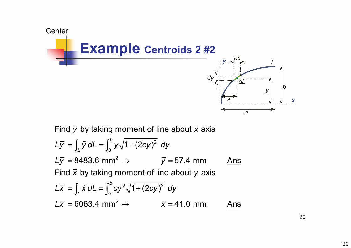
Example Centroids 2 #2
Center
Example Centroids 2 #2
Find by taking moment of line about axisb
y x
= = +
= → =
2
02
1 (2 )
8483.6 mm 57.4 mm Ans
b
LLy y dL y cy dy
Ly y
= = + 2 2
0
Find by taking moment of line about axis
1 (2 ) b
L
x y
Lx x dL cy cy dy
20
= → = 0
26063.4 mm 41.0 mm AnsL
Lx x
21
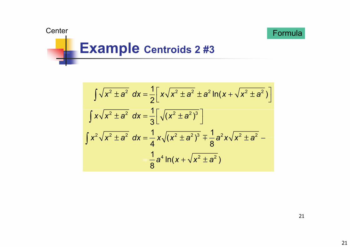
Example Centroids 2 #3
Center Formula
Example Centroids 2 #3
2 2 2 2 2 2 21 ln( )21
x a dx x x a a x x a ± = ± ± + ±
2 2 2 2 3
2 2 2 2 2 3 2 2 2
1 ( )31 1( )
x x a dx x a
x x a dx x x a a x x a
± = ±
± = ± ±
4 2 2
( )4 81 ln( )8
x x a dx x x a a x x a
a x x a
± = ± ± −
+ ±=
8
21
22
Example Centroids 3 #1
Center
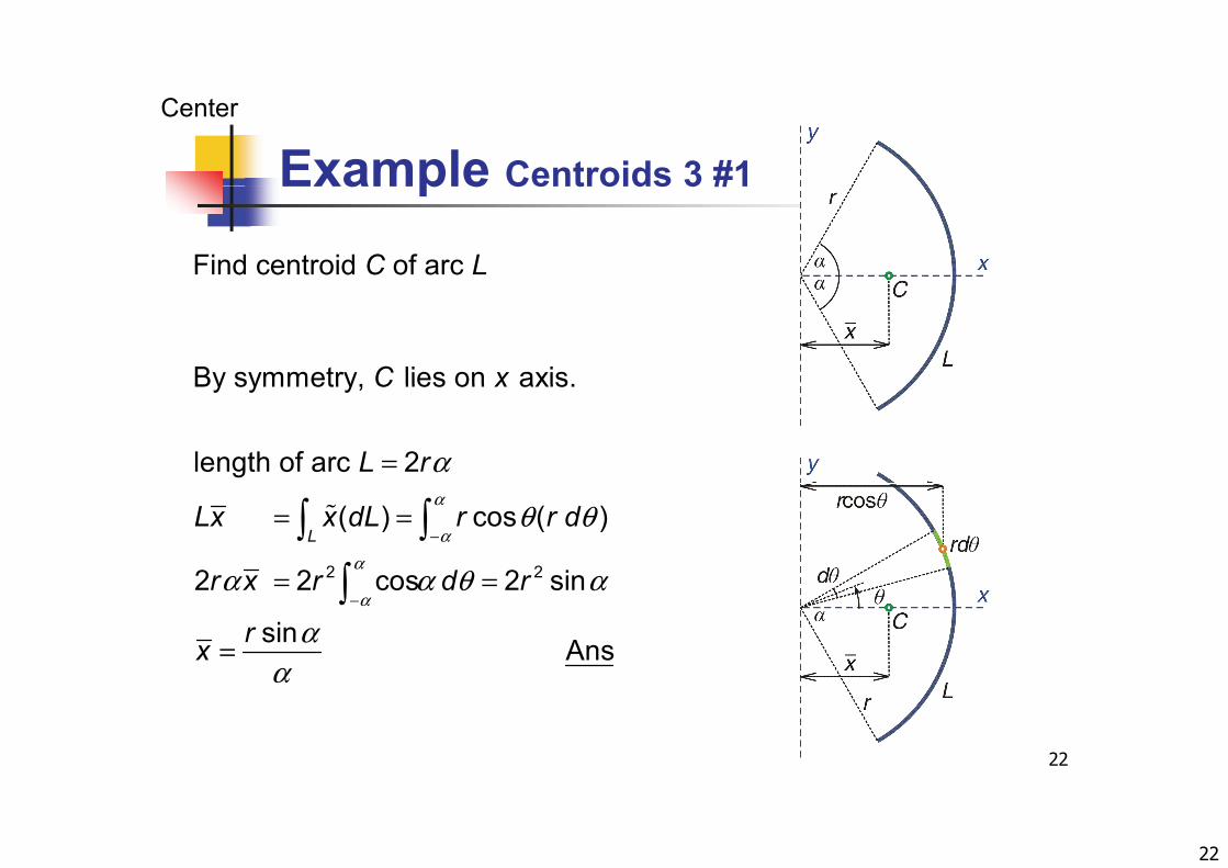
Example Centroids 3 #1
Find centroid C of arc L
By symmetry, lies on axis.C x
α=
By symmetry, lies on axis.
length of arc 2
C x
L rα
αα
θ θ
α α θ α
−
= =
= =
2 2
( ) cos ( )
2 2 cos 2 sin
LLx x dL r r d
r x r d rα
α α θ α
αα
−= =
=
2 2 cos 2 sin
sin Ans
r x r d r
rx
22
α
23
Example Centroids 4 #1
Center
Example Centroids 4 #1
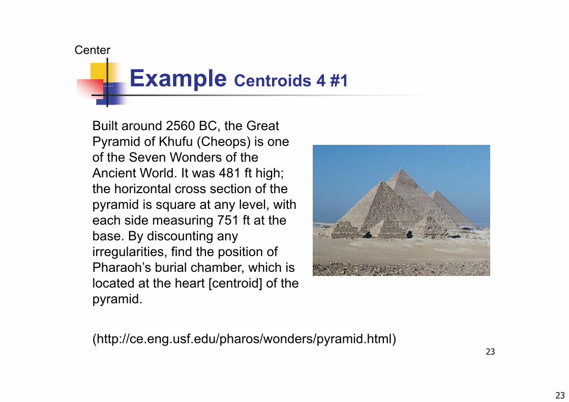
Built around 2560 BC, the Great Pyramid of Khufu (Cheops) is one of the Seven Wonders of the Ancient World. It was 481 ft high; g ;the horizontal cross section of the pyramid is square at any level, with each side measuring 751 ft at theeach side measuring 751 ft at the base. By discounting any irregularities, find the position of Pharaoh’s burial chamber which isPharaoh s burial chamber, which is located at the heart [centroid] of the pyramid.
23(http://ce.eng.usf.edu/pharos/wonders/pyramid.html)
24
Example Centroids 4 #2
Center
Example Centroids 4 #2
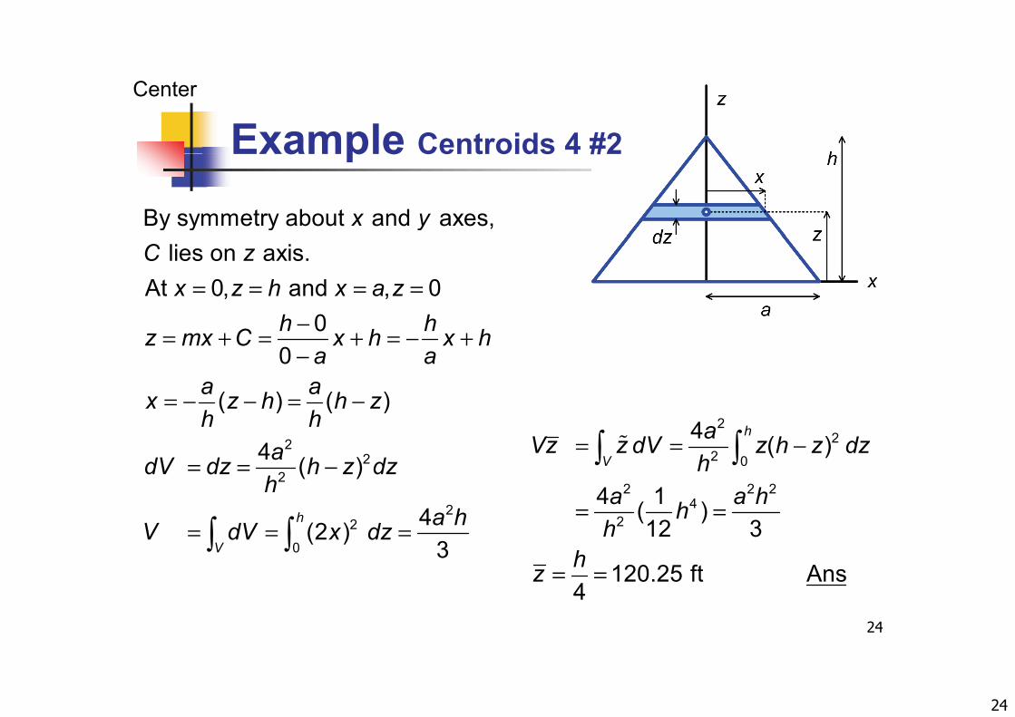
By symmetry about and axes, x y lies on axis.
At 0, and , 00
C zx z h x a z
h h= = = =
00
( ) ( )
h hz mx C x h x ha a
a ax z h h z
−= + = + = − +−
= =
22
2
( ) ( )
4 ( )
x z h h zh h
adV dz h z dzh
= − − = −
= = −
22
2 0
4 ( )h
V
aVz z dV z h z dzh
= = −
2
22
0
4(2 ) 3
h
V
ha hV dV x dz= = =
2 2 24
24 1( )
12 3a a hh
hh
= =
24
120.25 ft Ans4hz = =
25
Example Centroids 5 #1
Center
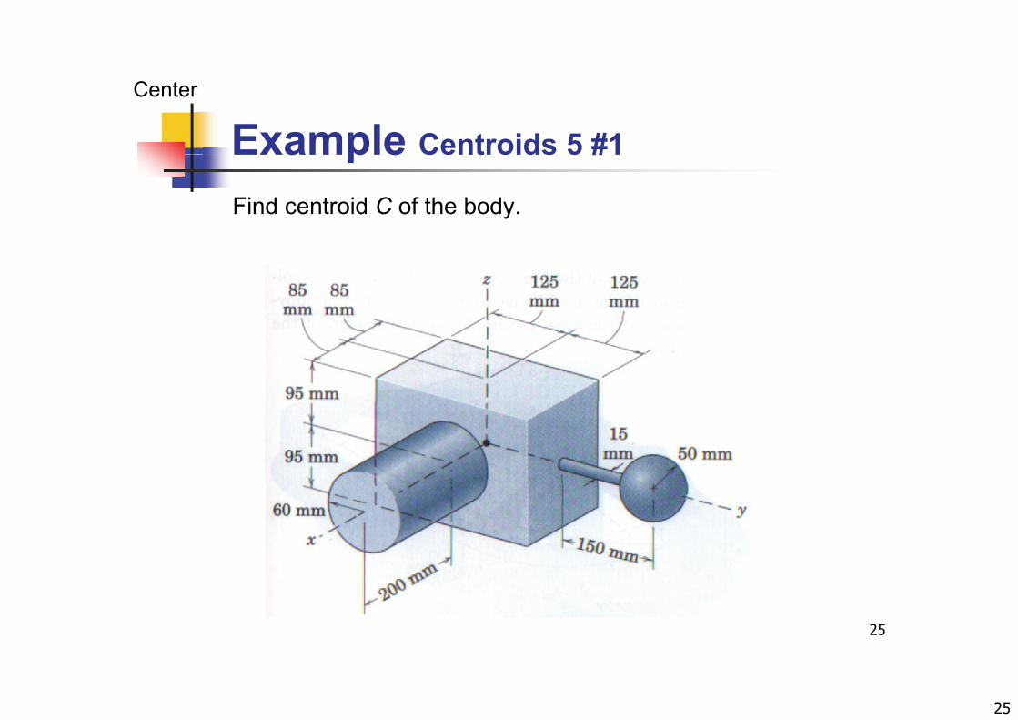
Example Centroids 5 #1
Find centroid C of the body.
25
26
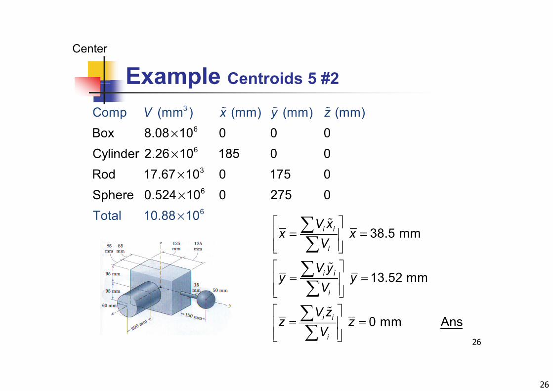
Example Centroids 5 #2
Center
Example Centroids 5 #2
6
3
B 8 08 10 0 0 0Comp (mm ) (mm) (mm) (mm)V x y z
×××
6
6
3
Box 8.08 10 0 0 0Cylinder 2.26 10 185 0 0Rod 17 67 10 0 175 0×
×× 6
6
Rod 17.67 10 0 175 0Sphere 0.524 10 0 275Total 1 10
00 88 ×Total 1 100.88
= =
38.5 mmi i
i
V xx x
V
= =
13.52 mmi i
i
V yy y
V
V
26
= =
0 mm Ansi i
i
V zz z
V

27
Pappus Theorems Formula #1Theorem IPappus
Pappus Theorems Formula #1
The area of a surface of revolution equals the product of the length of the generating curve and the distancethe length of the generating curve and the distance traveled by the centroid of the curve in generating the surface area.
For surface area generated bycomplete revolutioncomplete revolution
(2 )( )S x Lπ=
2S LFor incomplete revolutionS
π= 2S xL
27
S xLθ=
28
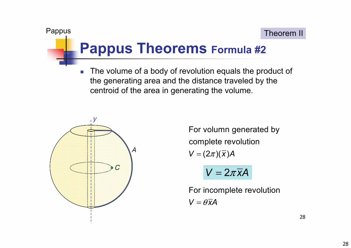
Pappus Theorems Formula #2
Pappus Theorem II
Pappus Theorems Formula #2
The volume of a body of revolution equals the product of the generating area and the distance traveled by thethe generating area and the distance traveled by the centroid of the area in generating the volume.
For volumn generated bycomplete revolution
(2 )( )V x Aπ=
For incomplete revolution
2V xAπ=
28
V xAθ=
29
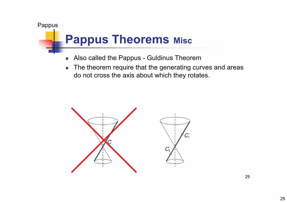
Pappus Theorems Misc
Pappus
Pappus Theorems Misc
Also called the Pappus - Guldinus TheoremThe theorem require that the generating curves and areas The theorem require that the generating curves and areas do not cross the axis about which they rotates.
29
30
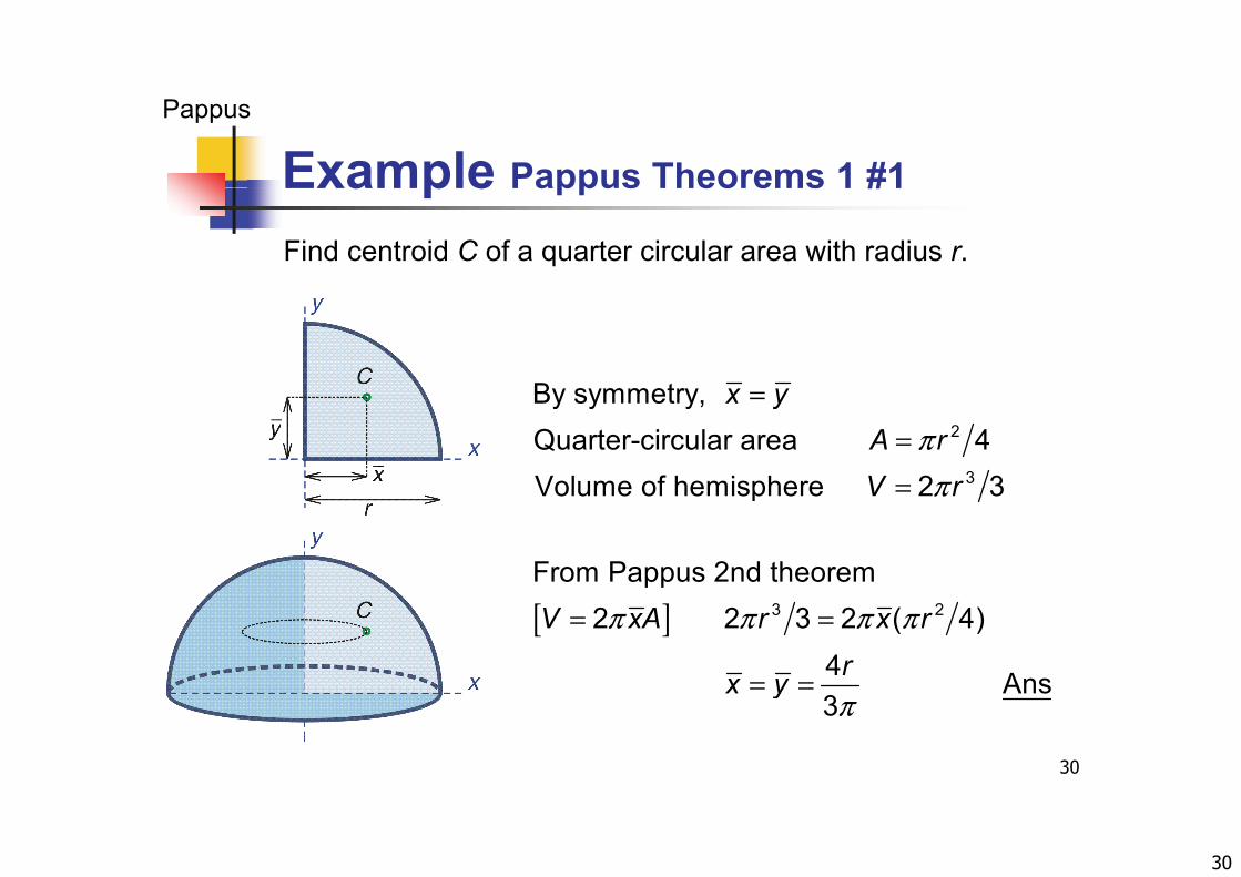
Example Pappus Theorems 1 #1
Pappus
Example Pappus Theorems 1 #1
Find centroid C of a quarter circular area with radius r.
By symmetry x yπ
π
===
2
3
By symmetry, Quarter-circular area 4Volume of hemisphere 2 3
x yA rV rπ=Volume of hemisphere 2 3
From Pappus 2nd theorem
V r
[ ]π π π π= =
= =
3 22 2 3 2 ( 4)4 Ans
V xA r x rrx y
30
π= = Ans
3x y
31
SummarySummary Centroid, CM and CG are centers of geometry, mass and gravity.
Centroid and CM coincide if the density ρ is constant. CM and CG coincide if g is constant.
Calculation by moment Integration Composite body
P th f b di t d b l ti Pappus theorems for bodies generated by revolutions
31
32
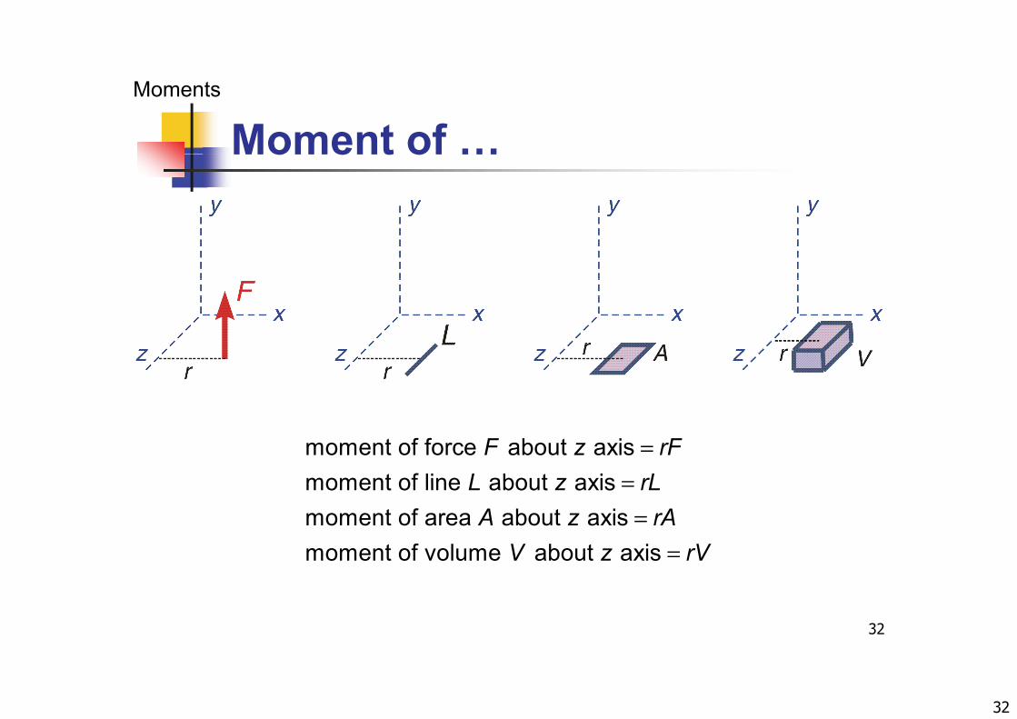
Moment of …Moments
Moment of …
moment of force about axismoment of line about axis
F z rFL z rL
==moment of line about axis
moment of area about axismoment of volume about axis
L z rLA z rA
V z rV
==
=
32

33
First Moment of Area Qx & Qy
Moments
First Moment of Area Qx & Qy The first moment of area Q
The first moment of area with The first moment of area with respect to x axes
Q dA A
The first moment of area with
xQ y dA yA= =
The first moment of area with respect to y axes
Q dA A yQ x dA xA= =
33
34
Second Moment of Area Ixx & Iyy
Moments
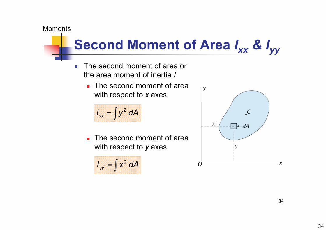
Second Moment of Area Ixx & Iyy The second moment of area or
the area moment of inertia Ithe area moment of inertia I The second moment of area
with respect to x axes
2
xxI y dA=
The second moment of area with respect to y axes
2
yyI x dA=
34
35
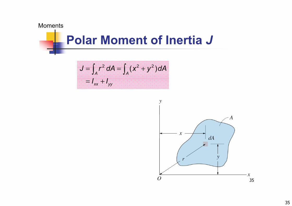
Polar Moment of Inertia JMoments
Polar Moment of Inertia J
2 2 2( )J r dA x y dA+ ( )A A
xx yy
J r dA x y dA
I I
= = +
= +
35

36
Ix & Iy vs Iz Parallel-Axis Theorem
Moments
Ix & Iy vs Iz Parallel Axis Theorem
2( )I y d dA′= +2 2
2
( )
( ) 2
0
xx yA
y yA A A
I y d dA
y dA d y dA d dA
I Ad
= +
′ ′= + +
+ +
20x x yI Ad′ ′= + +
2xx x x yI I Ad′ ′= +
2yy y y x
xx yy
I I AdJ I I
′ ′= += +
36
37
Example Second Moment of Area 1 #1
Moments
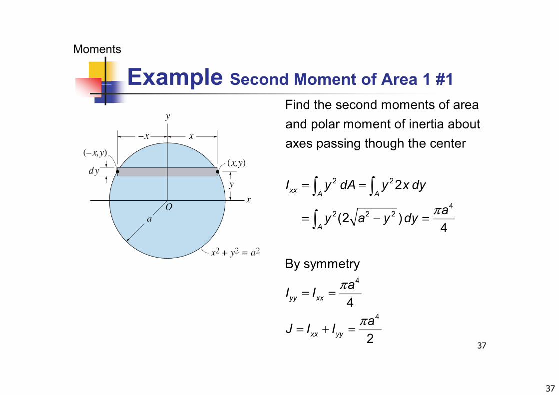
Example Second Moment of Area 1 #1Find the second moments of areaand polar moment of inertia aboutpaxes passing though the center
2 2
42 2 2
2
(2 )
xx A AI y dA y x dy
ay a y dyI π
= =
= − =
(2 )4
By symmetry
Axx y a y dyI = =
4
By symmetry
4yy xxaI I π= =
37
4
2xx yyaJ I I π= + =
38
Example Second Moment of Area 1 #2
Moments
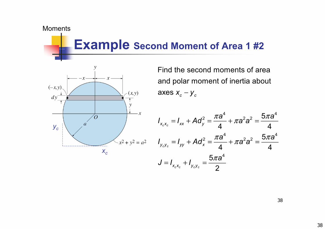
Example Second Moment of Area 1 #2
Find the second moments of area and polar moment of inertia aboutaxes c cx y−
4 42 2 2 5
4 4c cx x xx ya aI I Ad a aπ ππ= + = + =
y4 4
2 2 2
4 45
4 4c cy y yy xa aI I Ad a aπ ππ= + = + =
xc
yc
452c c c cx x y yaJ I I π= + =
c
38
39
Table Centroid and Moment of Inertia #1
Moments
Table Centroid and Moment of Inertia #1
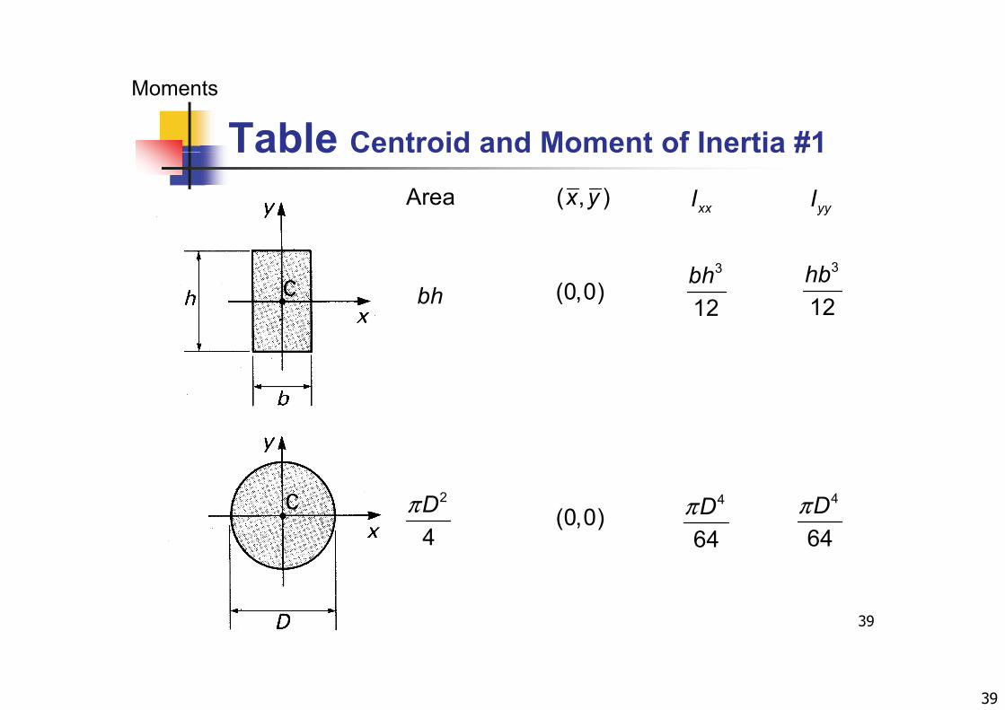
( , )x y xxI yyIArea
bh (0,0)3
12bh 3
12hb
12 12
2
4Dπ (0,0)
4
64Dπ 4
64Dπ
39

40
Table Centroid and Moment of Inertia #2
Moments
Table Centroid and Moment of Inertia #2
( , )x y xxI yyIArea
bh(0 )h 3bh 3hb
2(0, )
3 36 48
abπ (0,0)3
4abπ 3
4baπ
40
41
Example Hibbeler 6-68 Mech of Mat #1
Moments
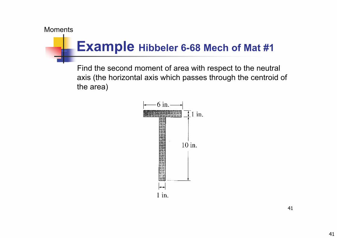
Example Hibbeler 6 68 Mech of Mat #1
Find the second moment of area with respect to the neutral axis (the horizontal axis which passes through the centroid ofaxis (the horizontal axis which passes through the centroid of the area)
41
42
Example Hibbeler 6-68 Mech of Mat #2
Moments
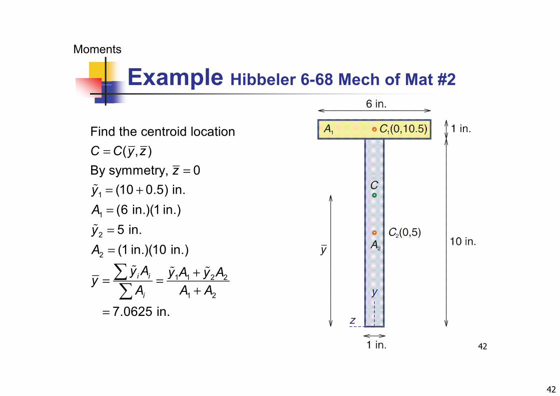
Example Hibbeler 6 68 Mech of Mat #2
Find the centroid locationFind the centroid location( , )
By symmetry, 0C C y z
z=
=
1
1
y y y,(10 0.5) in.(6 in.)(1 in.)
yA
= +=
2
2
5 in.(1 in.)(10 in.)
yA
A
==
1 1 2 2
1 2
7 0625 in
i i
i
y A y A y Ay
yA A A
+= =+
=
42
7.0625 in.y =
43
Example Hibbeler 6-68 Mech of Mat #3
Moments
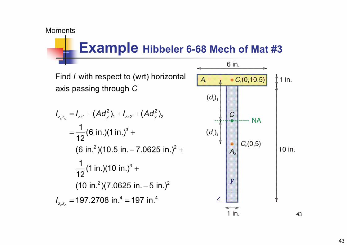
Example Hibbeler 6 68 Mech of Mat #3
Find with respect to (wrt) horizontal I p ( )axis passing through C
2 21 1 2 2
3
( ) ( )
1 (6 in.)(1 in.)12c c
c c
z z
z z zz y zz yI I Ad I
I
Ad= + + +
= +
2 2
3
12(6 in. )(10.5 in. 7.0625 in.)
1
c c
c c
z z
z zI = − +
3
2
1 (1 in.)(10 in.)12(10 in. )(7.0
c c
c c
z z
z zI
I =
=
+
2625 in. 5 in.)−
43
4 4197.2708 in. 197 in.c cz zI = =
44
Loads Concentration vs. Distribution
Distributed Loads
Loads Concentration vs. Distribution
Concentrated Load acts at a point, does not exist in the exact sense,
t bl i ti h t t i ll acceptable approximation when contact area is small.
Distributed Loads distributed over line, area, volume.
44

45
Loads Hand Tools
Distributed Loads
Loads Hand Tools
Blacksmith Hammer Wood ChiselBlacksmith Hammer Wood Chisel
45
46
Loads Distribution Types
Distributed Loads
Loads Distribution Types
Line DistributionIntensity w (N/m) = force per unit length Intensity w (N/m) = force per unit length
Area Distribution Intensity (N/m2 or Pa) = force per unit area Action of fluid force pressure
I t l i t it f f i lid t Internal intensity of force in solid stress
Volume DistributionVolume Distribution Intensity (N/m3) = body force per unit volume Specific weight ρg is the intensity of gravitational
tt ti
46
attraction.
47
Loads Resultant Force System
Distributed Loads
Loads Resultant Force System
Distributed loads can be represented by an equivalent force-couple system consisting offorce-couple system, consisting of Resultant force FR
Magnitude Direction Line of action
Resultant couple M Resultant couple MR
Magnitude Direction
47
48
Line Distribution Descriptions
Distributed Loads
Line Distribution Descriptions
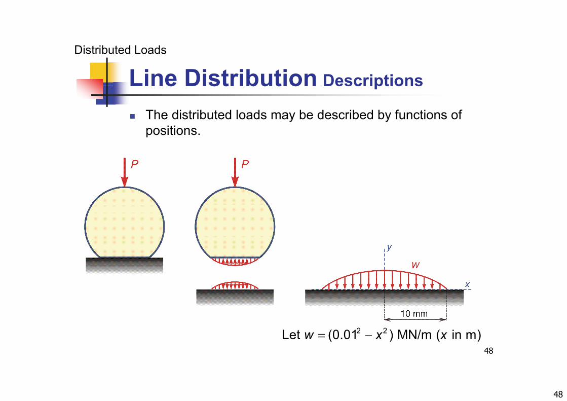
The distributed loads may be described by functions of positionspositions.
48
2 2Let (0.01 ) MN/m ( in m)w x x= −
49
Line Distribution Resultants
Distributed Loads
Line Distribution Resultants
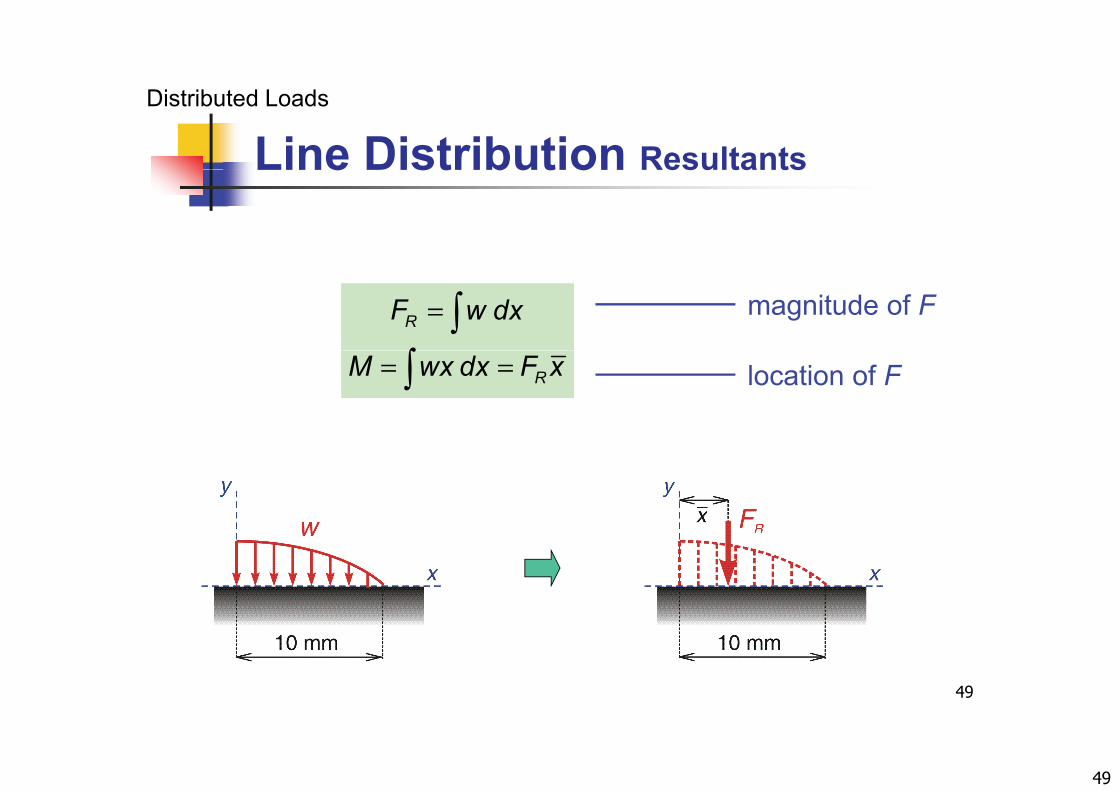
RF w dx=
magnitude of F
RM wx dx F x= = location of F
49
50
Example Line Resultant 1 #1
Distributed Loads
p
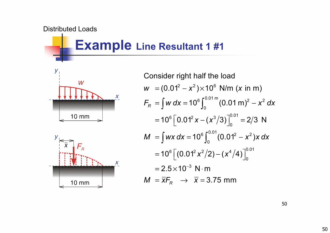
Consider right half the load= − ×
= = −
2 2 6
0.01 m6 2 2
Consider right half the load(0.01 ) 10 N/m ( in m)
10 (0 01 m)
w x x
F w dx x dx= = −
= − =
0
0.016 2 3
0
10 (0.01 m)
10 0.01 ( 3) 2 3 N
RF w dx x dx
x x
= = −
= −
0.016 2 2
00.016 2 2 4
10 (0.01 )
10 (0.01 2) ( 4)
M wx dx x x dx
x x−
= × ⋅=
03
0 (0 0 ) ( )
2.5 10 N mM xF → = 3.75 mmR x
50
R
51
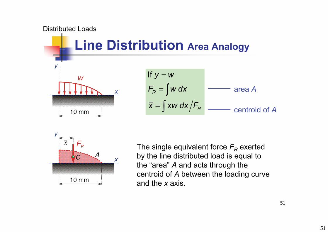
Line Distribution Area Analogy
Distributed Loads
Line Distribution Area Analogy
If y w=
If
R
y w
F w dx
d F
=
area A
Rx xw dx F= centroid of A
The single equivalent force FR exerted by the line distributed load is equal toby the line distributed load is equal to the “area” A and acts through the centroid of A between the loading curve and the x axis
51
and the x axis.
52
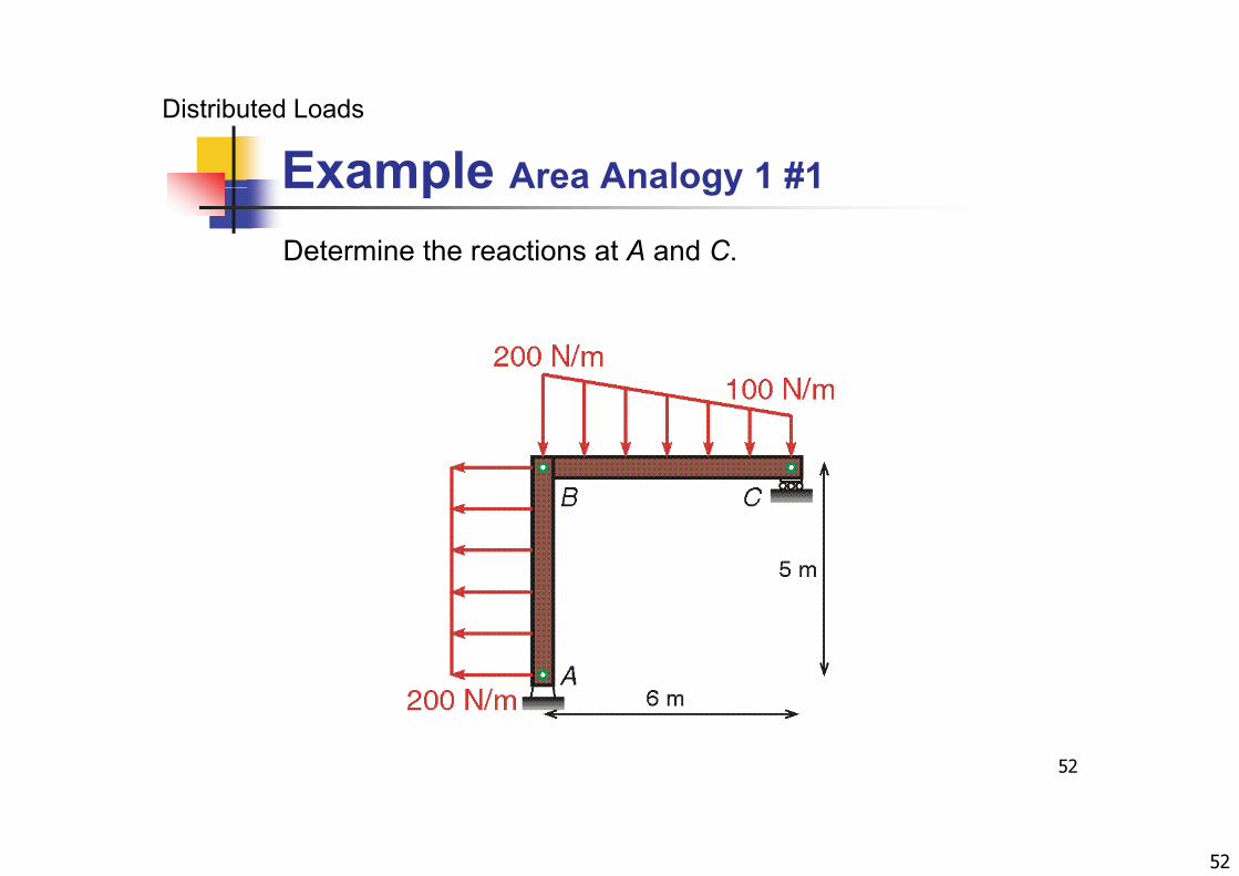
Example Area Analogy 1 #1
Distributed Loads
Example Area Analogy 1 #1
Determine the reactions at A and C.
52
53
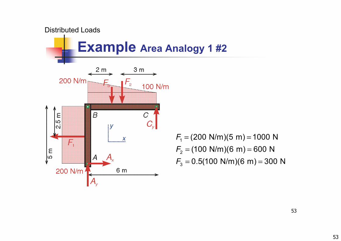
Example Area Analogy 1 #2
Distributed Loads
Example Area Analogy 1 #2
(200 N/ )(5 ) 1000 NF1
2
(200 N/m)(5 m) 1000 N(100 N/m)(6 m) 600 N0 5(100 N/m)(6 m) 300 N
FFF
= == == =3 0.5(100 N/m)(6 m) 300 NF = =
53
54
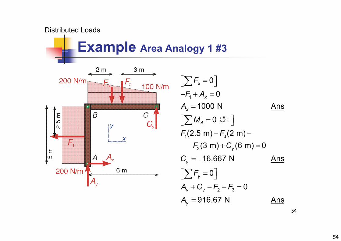
Example Area Analogy 1 #3
Distributed Loads
Example Area Analogy 1 #3
0F 1
0
01000 N Ans
x
x
F
F AA
= − + =
=
1000 N Ans
0
(2 5 m) (2 m)
x
A
A
M
F F
=
= + − −
1 3
2
(2.5 m) (2 m)(3 m) (6 m) 016.667 N Ans
y
y
F FF C
C
+ =
= −
2 3
0
0
y
y
y y
F
A C F F
= + − − =
54
2 3 0916.67 N Ans
y y
y
C
A =

55
Example Area Analogy 2 #1
Distributed Loads
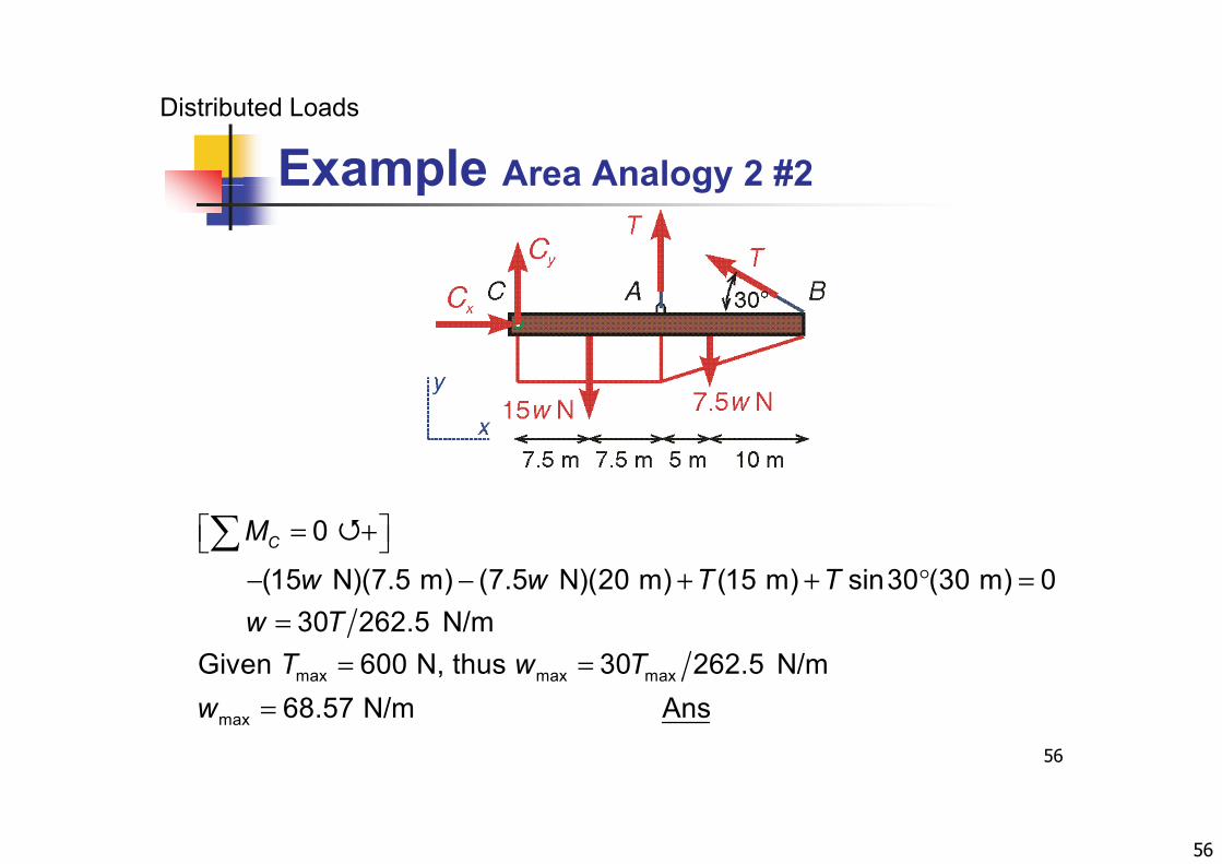
Example Area Analogy 2 #1
If the cable can sustain tension of up to 600 N, determine the maximum wthe maximum w.
55
56
Example Area Analogy 2 #2
Distributed Loads
Example Area Analogy 2 #2
= + + + ° =
0
(15 N)(7 5 m) (7 5 N)(20 m) (15 m) sin30 (30 m) 0CM
w w T T
− − + + ==
= =max max max
(15 N)(7.5 m) (7.5 N)(20 m) (15 m) sin30 (30 m) 030 262.5 N/m
Given 600 N, thus 30 262.5 N/m
w w T Tw T
T w T
56
=max max max
max 68.57 N/m Answ
57
Example Area Analogy 3 #1
Distributed Loads
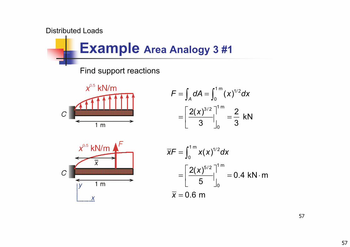
Example Area Analogy 3 #1
Find support reactions
1 m 1/ 2
01 m3 / 2
( )
2( ) 2
AF dA x dx= =
3 / 2
0
2( ) 2 kN3 3x
= =
1 m 1/ 2
01 m5/ 2
( )xF x x dx=
1 m5 / 2
0
2( ) 0.4 kN m5
0 6 m
x
x
= = ⋅
57
0.6 mx =
58
Example Area Analogy 3 #2
Distributed Loads
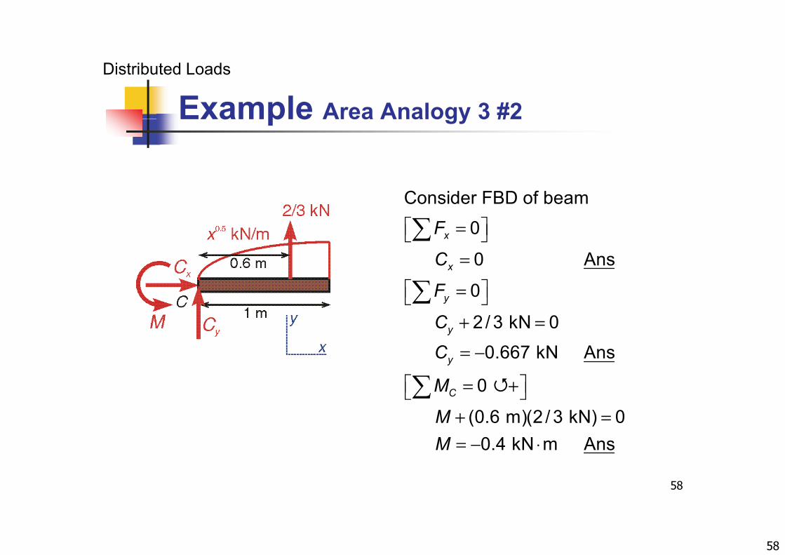
Example Area Analogy 3 #2
Consider FBD of beam
0xF = 0 Ans
0x
y
C
F
=
= 2 / 3 kN 0
0.667 kN Ansy
y
C
C
+ =
= −
0
(0.6 m)(2 / 3 kN) 0CM
M
= + + =
58
0.4 kN m AnsM = − ⋅
59
Area Distribution Resultants
Distributed Loads
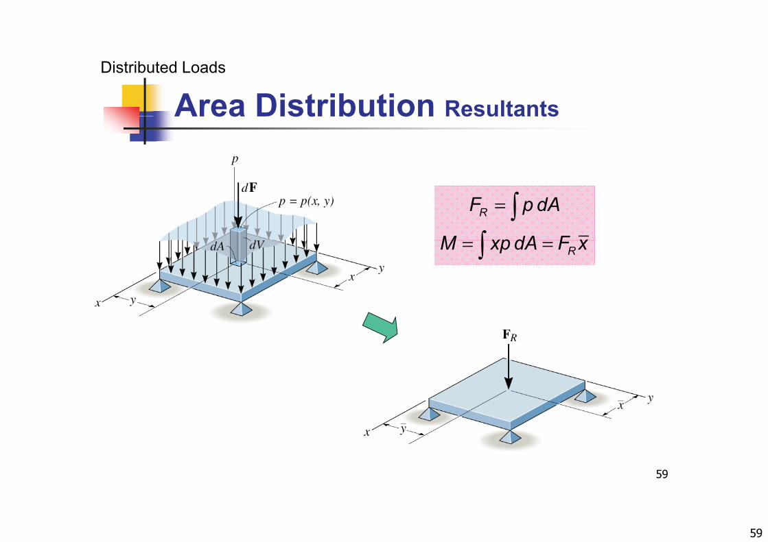
Area Distribution Resultants
RF p dA
M xp dA F x
= RM xp dA F x= =
59
60
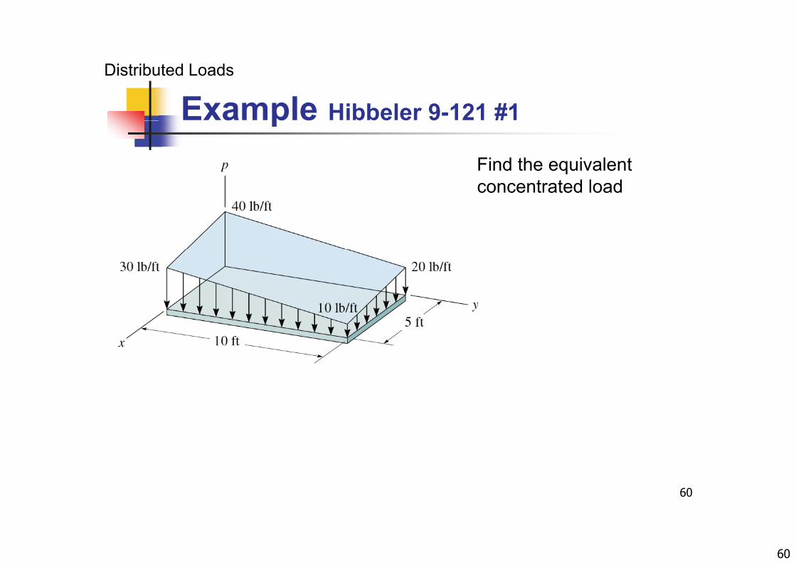
Example Hibbeler 9-121 #1
Distributed Loads
pFind the equivalent concentrated loadconcentrated load
60
61
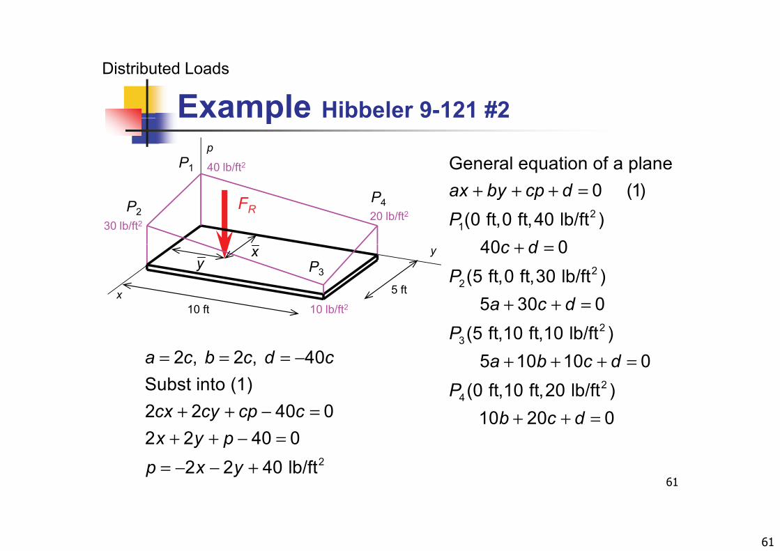
Example Hibbeler 9-121 #2
Distributed Loads
pp
40 lb/ft2 General equation of a planeP1
FR 20 lb/ft230 lb/ft2
21
0 (1)(0 ft,0 ft,40 lb/ft )
40 0
ax by cp dP
c d
+ + + =
+
P2P4
y
x10 lb/ft210 ft
5 ft
xy 2
2
40 0(5 ft,0 ft,30 lb/ft )
5 30 0
c dP
a c d
+ =
+ + =
P3
10 lb/ft210 ft2
3
5 30 0(5 ft,10 ft,10 lb/ft )
5 10 10 0
a c dP
a b c d
+ + =
+ + + =2 , 2 , 40a c b c d c= = = −2
4(0 ft,10 ft,20 lb/ft )10 20 0
Pb c d+ + =
Subst into (1)2 2 40 02 2 40 0cx cy cp c+ + − =
61
2
2 2 40 02 2 40 lb/ft
x y pp x y
+ + − == − − +
62
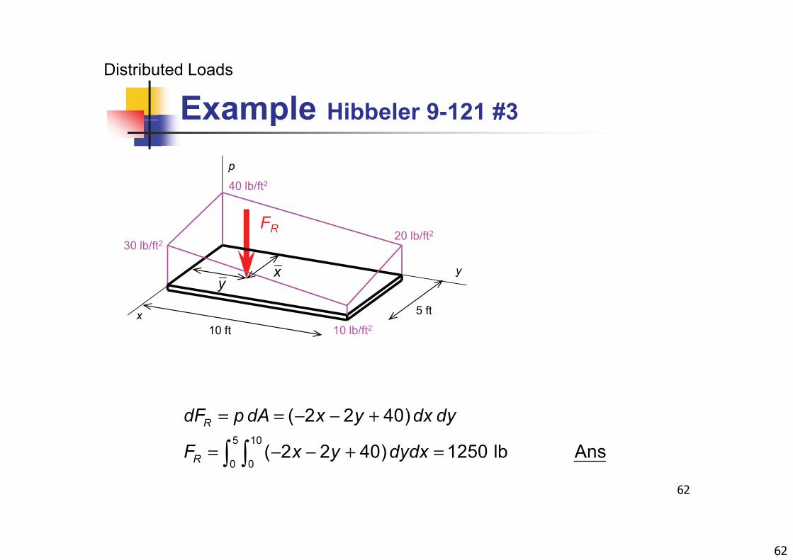
Example Hibbeler 9-121 #3
Distributed Loads
pp
40 lb/ft2
FR
40 lb/ft2
20 lb/ft230 lb/ft2
y
30 lb/ft
5 ft
xy
x10 lb/ft210 ft
5 ft
= = − − +
5 10
( 2 2 40)RdF p dA x y dx dy
62
= − − + =
5 10
0 0( 2 2 40) 1250 lb AnsRF x y dydx
63
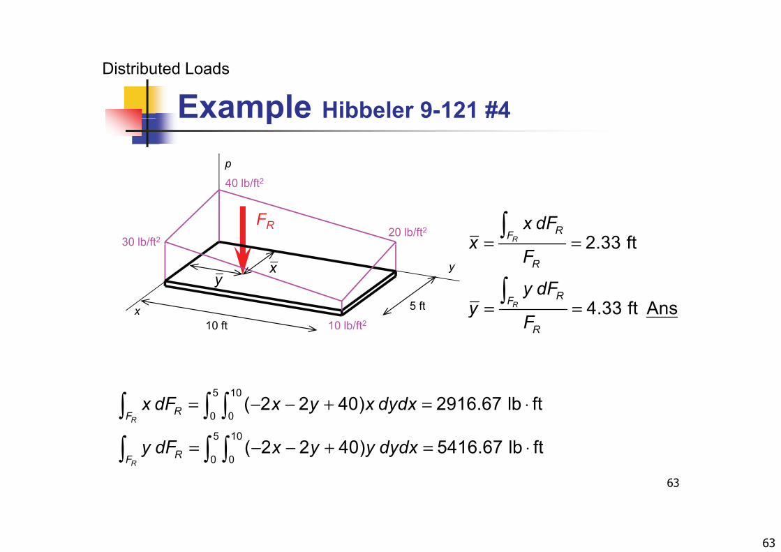
Example Hibbeler 9-121 #4
Distributed Loads
pp
40 lb/ft2
FR
40 lb/ft2
20 lb/ft230 lb/ft2 = =
2 33 ftRRF
x dFx
y
30 lb/ft
5 ft
xy
= =
= =
2.33 ft
4 33 ft AnsR
R
RF
xF
y dFyx
10 lb/ft210 ft
5 ft = = 4.33 ft AnsR
yF
5 10
0 0
5 10
( 2 2 40) 2916.67 lb ftR
RFx dF x y x dydx= − − + = ⋅
63
5 10
0 0( 2 2 40) 5416.67 lb ft
RRF
y dF x y y dydx= − − + = ⋅
64
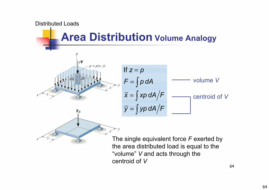
Area Distribution Volume Analogy
Distributed Loads
Area Distribution Volume Analogy
If z p
F p dA
=
= volume V
p
x xp dA F=
centroid of V
y yp dA F=
The single equivalent force F exerted by the area distributed load is equal to the
64
q“volume” V and acts through the centroid of V

65
Fluid StaticsFluid Statics
Fluid Statics Required in studies and designs of pressure vessels,
piping ships dams and off-shore structures etcpiping, ships, dams and off-shore structures, etc.
Topics Definitions Fluid pressure
Hydrostatic pressure on submerged surfaces Hydrostatic pressure on submerged surfaces Buoyancy Air pressurep
65
66
Fluid Statics Definitions
Fluid Statics
Fluid Statics Definitions
Fluid is any continuous substance which, when at rest, is unable to support shear forceunable to support shear force.
Fluid Statics studies pressure of fluid at rest. Hydrostatics – stationary liquid Aerostatics – stationary gas
Pascal’s Law: the pressure at any given point in a fluid is the same in all directionsthe same in all directions.
Pressure p in fluid at rest is a function of vertical dimension and its density ρ.
Resultant force on a body from pressure acts at the center of pressure P.
66
67
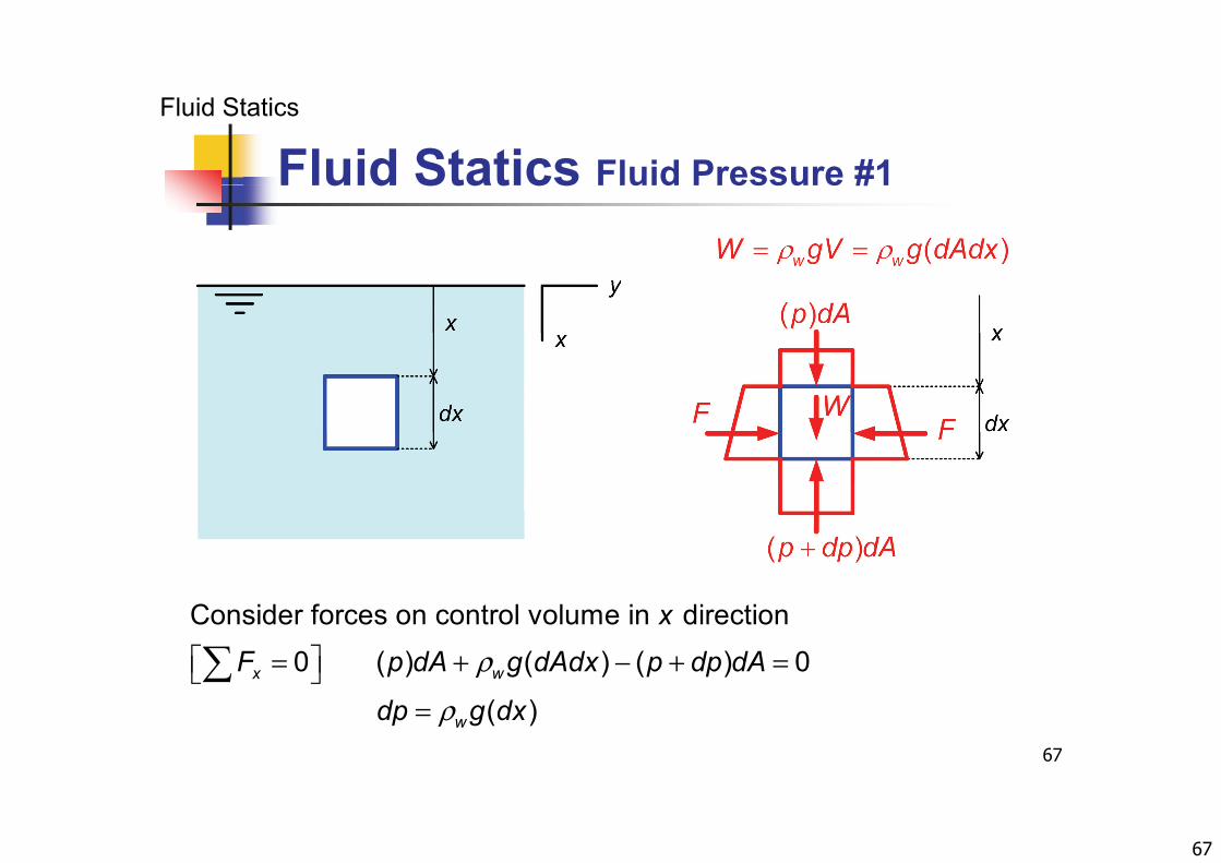
Fluid Statics Fluid Pressure #1
Fluid Statics
Fluid Statics Fluid Pressure #1
ρ = + − + = Consider forces on control volume in direction
0 ( ) ( ) ( ) 0x w
x
F p dA g dAdx p dp dA
67
ρ
=
( )x w
wdp g dx
68
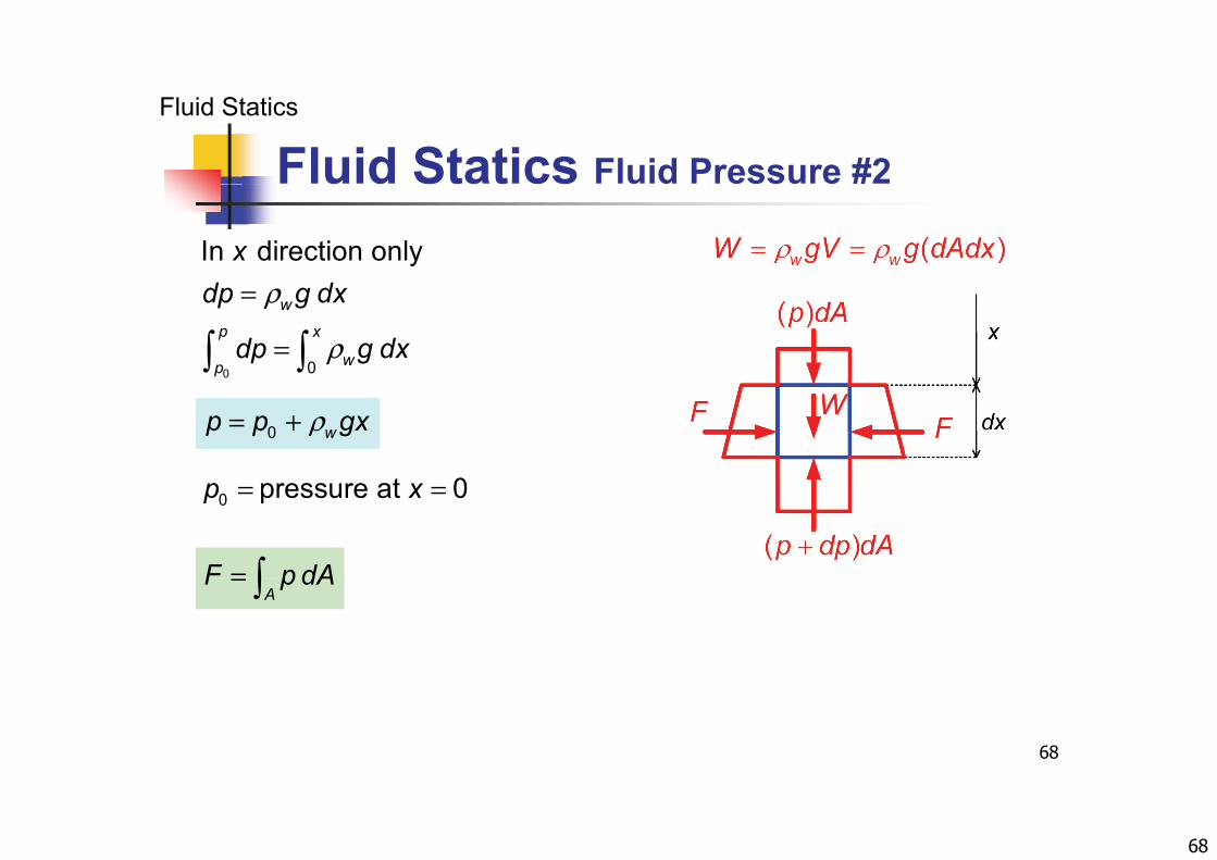
Fluid Statics Fluid Pressure #2
Fluid Statics
In direction onlyxd d
0 0
wp x
wp
dp g dx
dp g dx
ρ
ρ
=
=
t 0
ρ= +0 wp p gx
0 pressure at 0p x= =
F p dA= A
F p dA=
68
69
Pressure Submerged Surfaces #1
Fluid Statics
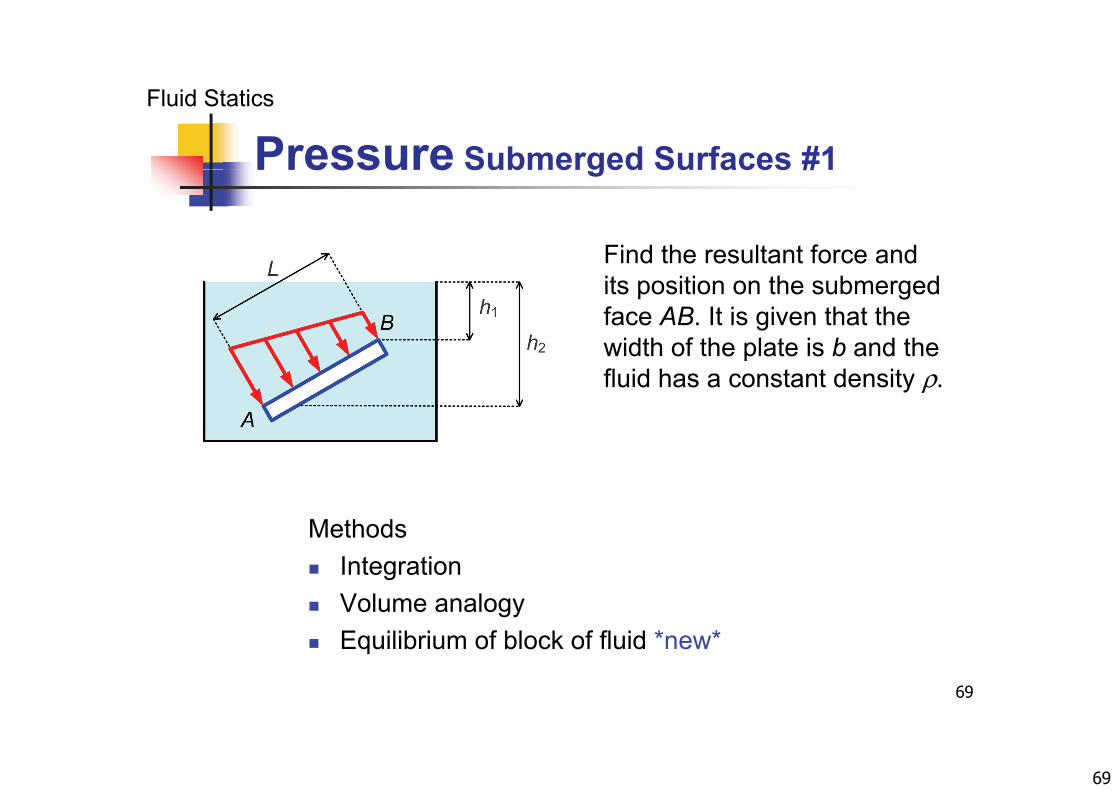
Pressure Submerged Surfaces #1
Find the resultant force andFind the resultant force and its position on the submerged face AB. It is given that the width of the plate is b and thewidth of the plate is b and the fluid has a constant density ρ.
MethodsMethods Integration Volume analogy
69
Equilibrium of block of fluid *new*
70
Pressure Submerged Surfaces #2
Fluid StaticsFluid Block
Pressure Submerged Surfaces #2
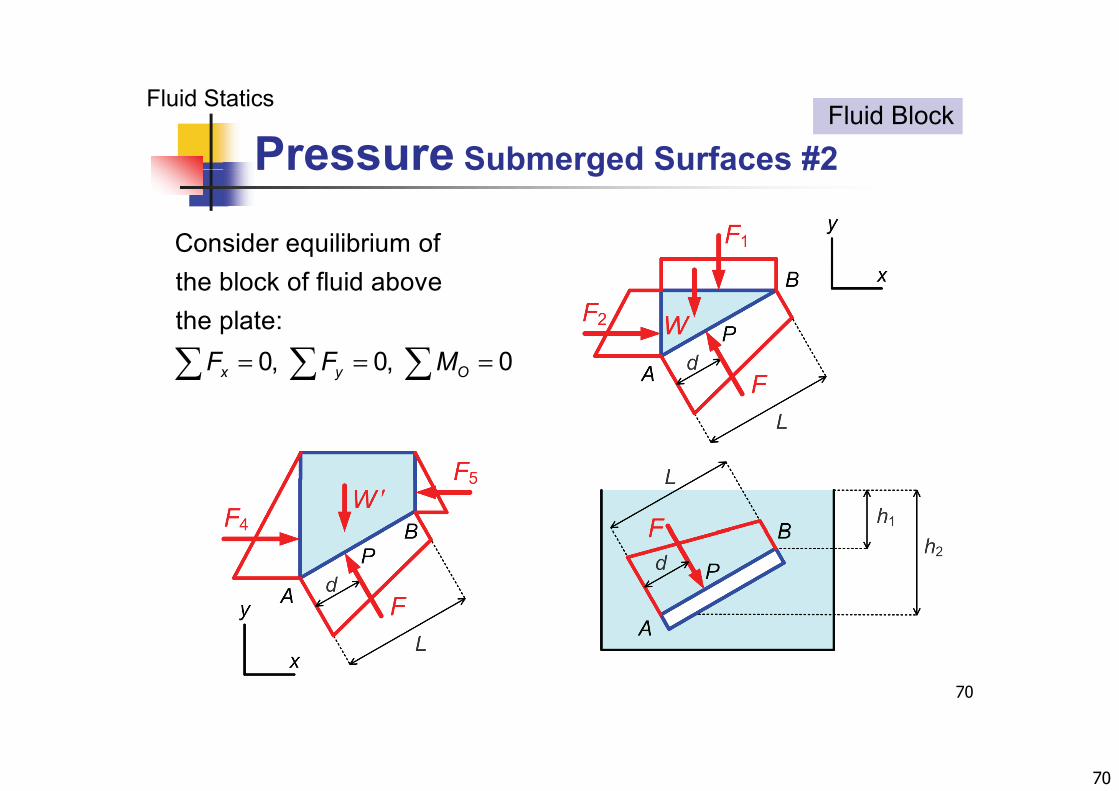
Consider equilibrium of
the block of fluid above the plate:
= = = 0, 0, 0x y OF F M
70
71
Example Fluid Statics 1 #1
Fluid Statics
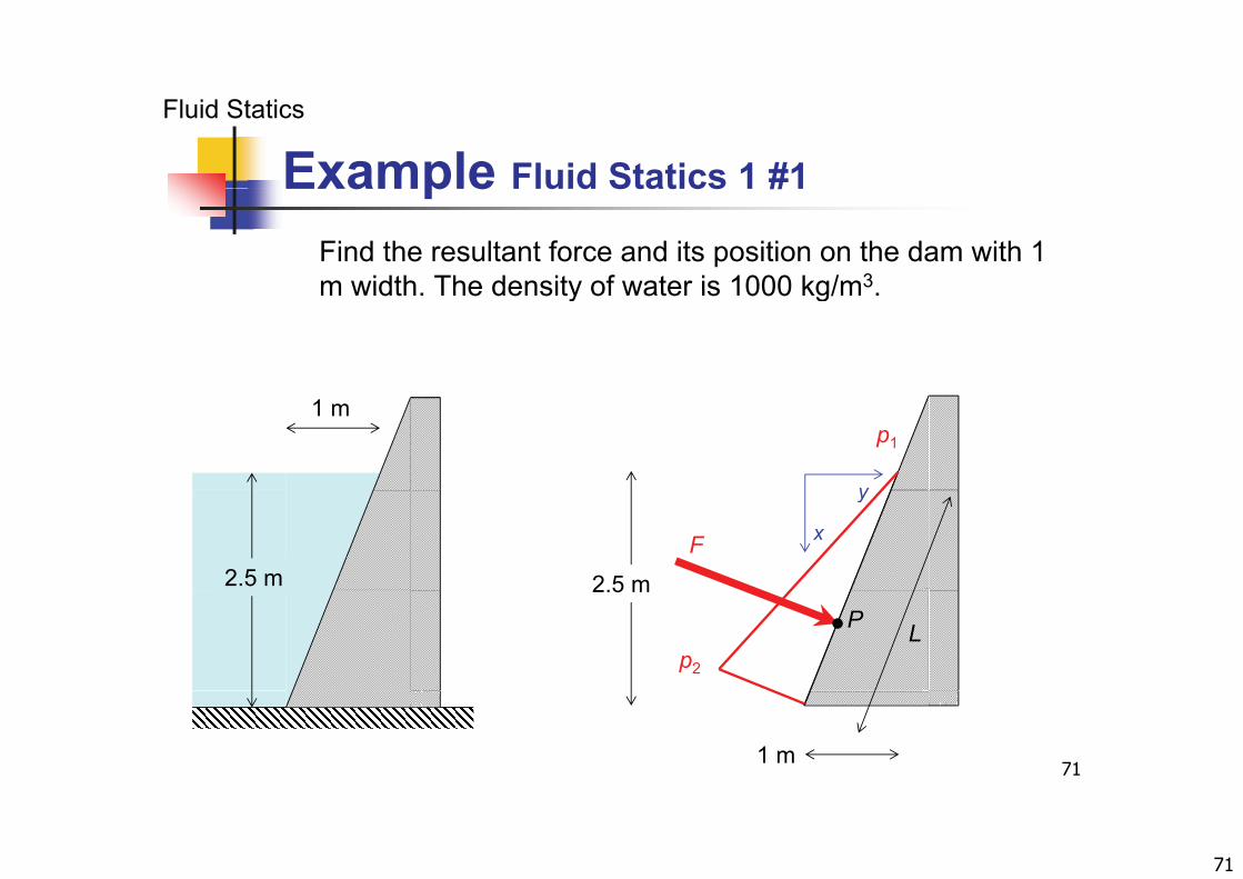
Example Fluid Statics 1 #1
Find the resultant force and its position on the dam with 1 m width The density of water is 1000 kg/m3m width. The density of water is 1000 kg/m .
1 m
y
p1
2.5 m 2.5 m
x
y
F
2.5 m
p2
LP
711 m
72
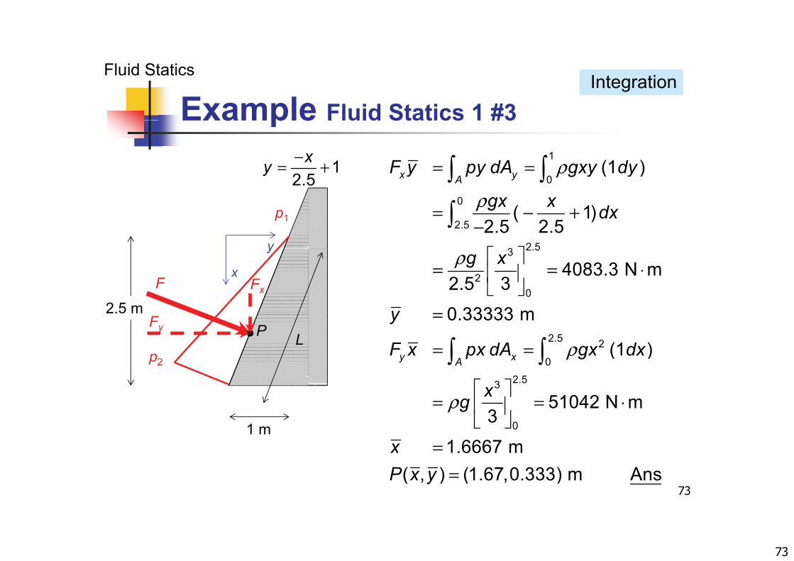
Example Fluid Statics 1 #2
Fluid StaticsIntegration
Example Fluid Statics 1 #2
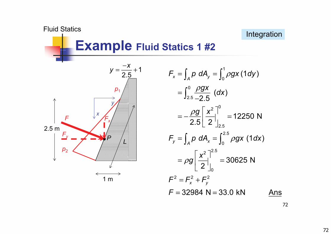
ρ= =
1(1 )x yF p dA gx dy1
2.5xy −= + ρ
ρ=−
0
0
2.5
( )
( )2.5
x yAp g y
gx dxy
p1
2.5
ρ = − =
02
2.5
12250 N2.5 2
g x
2.5 m
x
y
F Fx
ρ= =
2.5
02.52
(1 )
3062 N
y xAF p dA gx dx
x
2.5 m
p2
LPFy
ρ
= =
= +0
2 2 2
30625 N2
x y
xg
F F F1 m
72
= =32984 N 33.0 kN Ansx y
F
73
Example Fluid Statics 1 #3
Fluid StaticsIntegration
Example Fluid Statics 1 #3
ρ= =
1
0(1 )x yA
F y py dA gxy dy12.5
xy −= +
ρ= − +−
0
2.5
2 53
( 1)2.5 2.5gx x dx
y
p1
2.5
ρ = = ⋅
2.53
20
4083.3 N m32.5
0 33333 m
g x
y2.5 m
x
y
F Fx
ρ
=
= =
2.5 2
02 5
0.33333 m
(1 )y xA
y
F x px dA gx dx
2.5 m
p2
LPFy
ρ
= = ⋅
2.53
0
51042 N m3
1 6667
xg1 m
73
==1.6667 m
( , ) (1.67,0.333) m AnsxP x y
74
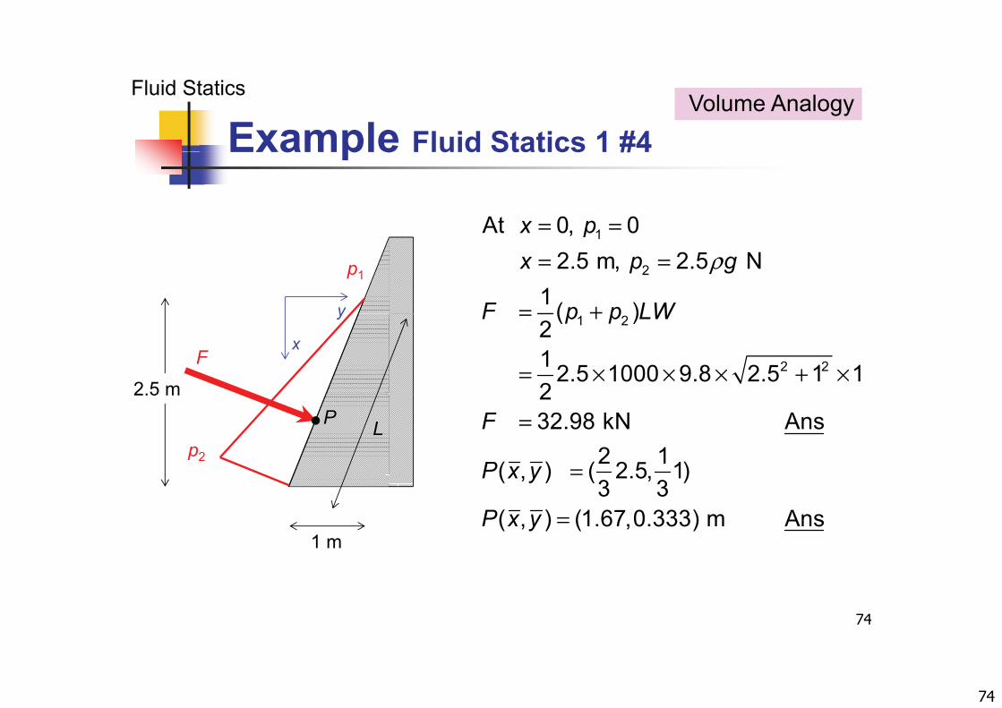
Example Fluid Statics 1 #4
Fluid StaticsVolume Analogy
Example Fluid Statics 1 #4
= =1At 0, 0x pρ= =
= +
1
2
At 0, 02.5 m, 2.5 N
1 ( )
x px p g
F p p LWy
p1
= +
= × × × + ×
1 2
2 2
( )21 2.5 1000 9.8 2.5 1 12
F p p LW
2.5 m
x
y
F
=
=
232.98 kN Ans
2 1( ) ( 2 5 1)
F
P x y
2.5 m
p2
LP
=
( , ) ( 2.5, 1)3 3
( , ) (1.67,0.333) m Ans
P x y
P x y1 m
74
75
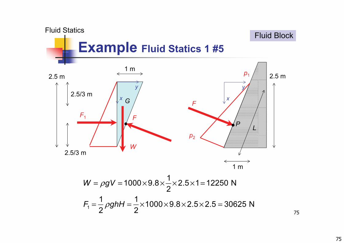
Example Fluid Statics 1 #5
Fluid StaticsFluid Block
Example Fluid Statics 1 #5
2.5 mp12.5 m1 m
x
y
Fx
y2.5/3 m
G
pLP
FF1
p2
W2.5/3 m
11000 9.8 2.5 1 12250 N2
W gVρ= = × × × × =
1 m
751
21 1 1000 9.8 2.5 2.5 30625 N2 2
F ghHρ= = × × × × =
76
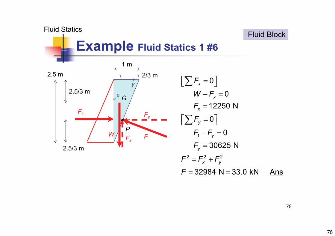
Example Fluid Statics 1 #6
Fluid StaticsFluid Block
Example Fluid Statics 1 #6
2.5 m
1 m
2/3 m =
− = 0
012250 N
x
x
F
W FF
x
y2.5/3 m
G=
= 12250 N
0
0
x
y
F
F
F F
F1
P
Fy
− =
=
+
1
2 2 2
0
30625 Ny
y
F F
F
F F F
FW
2.5/3 mFx
= +
= =32984 N 33.0 kN Ansx yF F F
F
76
77
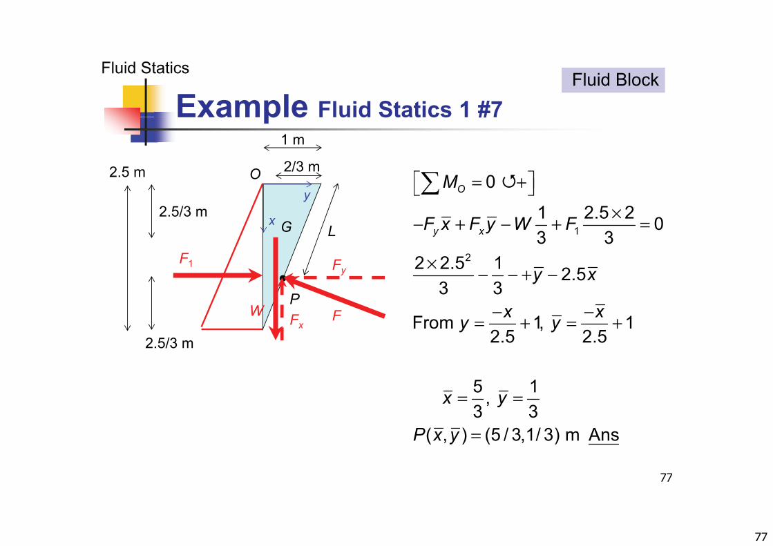
Example Fluid Statics 1 #7
Fluid StaticsFluid Block
Example Fluid Statics 1 #7
+ 0M 2.5 m
1 m
2/3 mO = + ×− + − + =
1
0
1 2.5 2 03 3
O
y x
M
F x F y W F
x
y2.5/3 m
G L
× − − + −2
3 32 2.5 1 2.5
3 3y x
F1
P
Fy
− −= + = +From 1, 12.5 2.5
x xy yFW
2.5/3 mFx
= =5 1, 3 3
( ) (5 / 3 1/ 3) A
x y
P
77
=( , ) (5 / 3,1/ 3) m AnsP x y
78
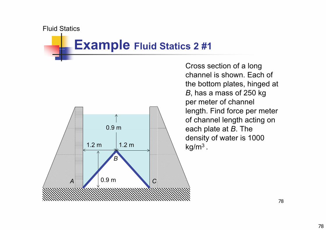
Example Fluid Statics 2 #1
Fluid Statics
Example Fluid Statics 2 #1
Cross section of a long channel is shown Each ofchannel is shown. Each of the bottom plates, hinged at B, has a mass of 250 kg per meter of channelper meter of channel length. Find force per meter of channel length acting on each plate at B The0 9 m each plate at B. The density of water is 1000 kg/m3 .1.2 m 1.2 m
0.9 m
0 9 mA C
B
78
0.9 mA C
79
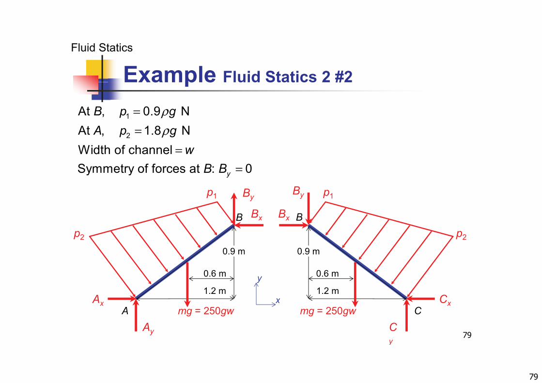
Example Fluid Statics 2 #2
Fluid Statics
Example Fluid Statics 2 #2
1At , 0.9 N A 1 8 N
B p gA
ρ=
2At , 1.8 NWidth of channelSymmetry of forces at : 0
A p gw
B B
ρ==
=Symmetry of forces at : 0yB B =
p1
B
By p1
B B
By
p2
0.9 m
BxBp2
0.9 m
Bx B
x
y1.2 m
A
0.6 m
1.2 mC
0.6 m
79
x
Ay
AxA mg = 250gw
Cy
CxCmg = 250gw
80
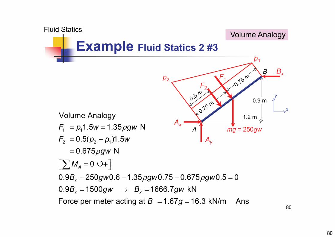
Example Fluid Statics 2 #3
Fluid StaticsVolume Analogy
Example Fluid Statics 2 #3
p2
p1
F1BxB
y
p2 F1F2
0.9 mx
1.2 mAx
A mg = 250gwρ= =1 1
Volume Analogy1.5 1.35 NF p w gw
Ay
g g
ρ= −=
2 2 10.5( )1.50.675 N
F p p wgw
ρ ρ
= + − − − =
0
0.9 250 0.6 1.35 0.75 0.675 0.5 00 9 1 00 1666
A
x
M
B gw gw gw
80
= → == =
0.9 1500 1666.7 kNForce per meter acting at 1.67 16.3 kN/m Ans
x xB gw B gwB g
81
Buoyancy Definition
Fluid Statics
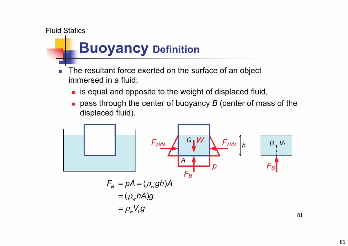
Buoyancy Definition
The resultant force exerted on the surface of an object immersed in a fluid:immersed in a fluid: is equal and opposite to the weight of displaced fluid, pass through the center of buoyancy B (center of mass of the
displaced fluid).
ρ= = ( )( )
B wF pA gh AhA
81
ρρ
==
( )w
w f
hA gV g
82
Buoyancy Stability
Fluid Statics
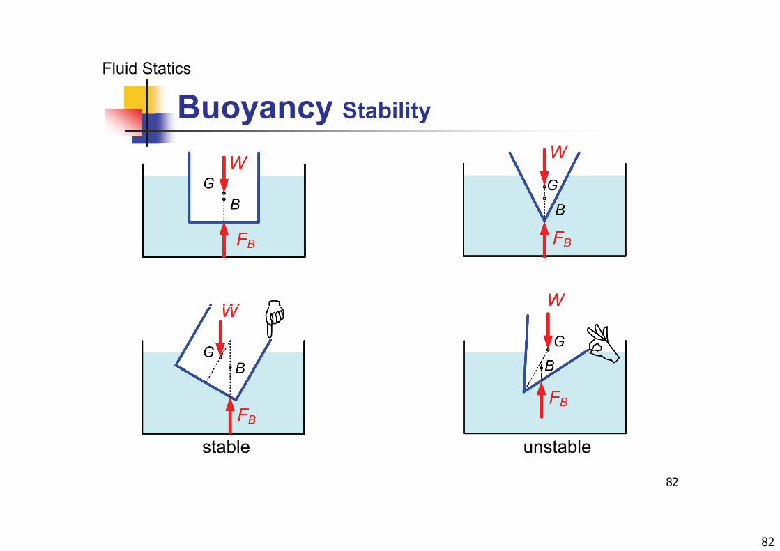
Buoyancy Stability
82
stable unstable
83
Flexible CablesCables
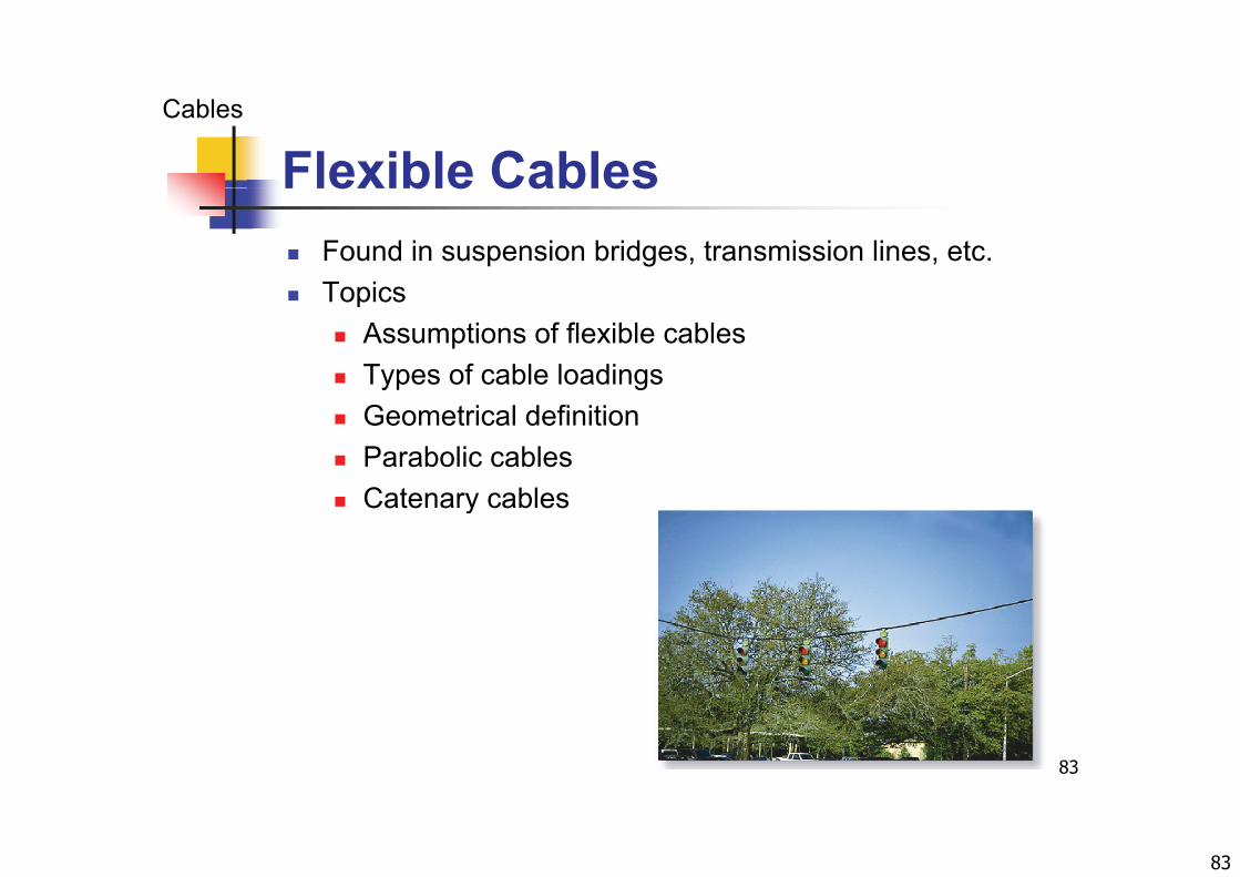
Flexible Cables Found in suspension bridges, transmission lines, etc.
Topics Topics Assumptions of flexible cables Types of cable loadingsyp g Geometrical definition Parabolic cables
C t bl Catenary cables
83
84
Flexible Cables Assumptions
Cables
Flexible Cables Assumptions
Bear load only in tensionNegligible displacement due to stretching Negligible displacement due to stretching Inextensible
Perfectly flexibley Negligible bending resistance Tangential tension along the cable
84
85
Flexible Cables Concentrated Loads
Cables
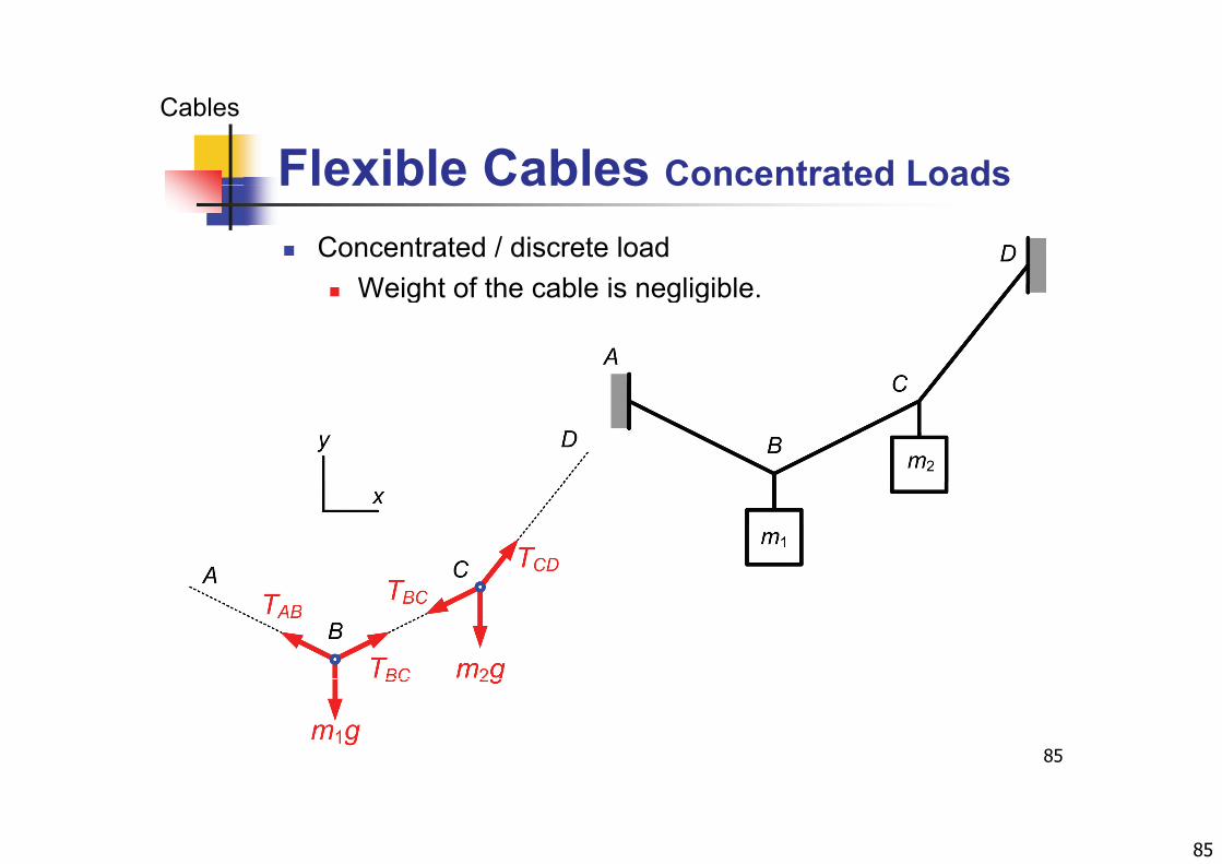
Flexible Cables Concentrated Loads
Concentrated / discrete loadWeight of the cable is negligible Weight of the cable is negligible.
85
86
Cables Geometrical Definitions
Cables
Cables Geometrical Definitions
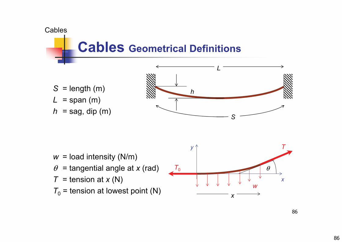
L
S = length (m)L = span (m)
h
h = sag, dip (m)S
w = load intensity (N/m)y T
θ = tangential angle at x (rad)T = tension at x (N)T = tension at lowest point (N)
x
T0
w
θ
86
T0 = tension at lowest point (N) x
87
Parabolic CablesCables
Parabolic Cables
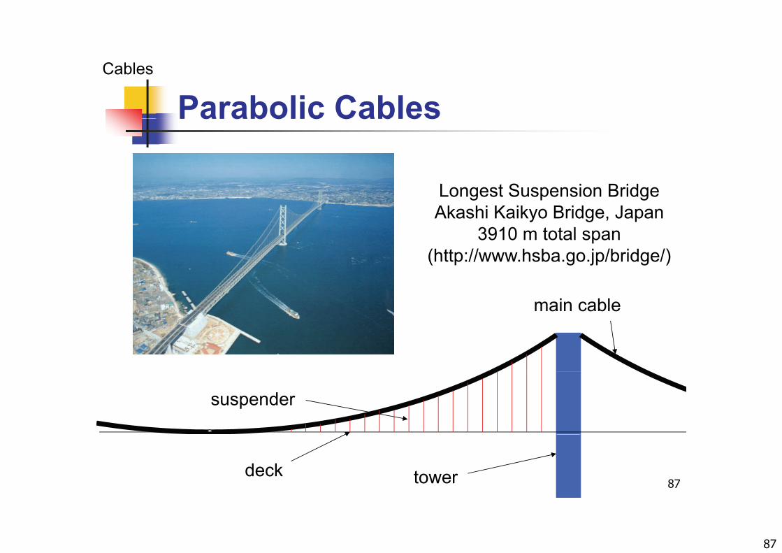
Longest Suspension BridgeAkashi Kaikyo Bridge, Japan
3910 m total span(http://www.hsba.go.jp/bridge/)
main cablemain cable
suspender
87towerdeck
88
Parabolic Cables Analysis
Cables
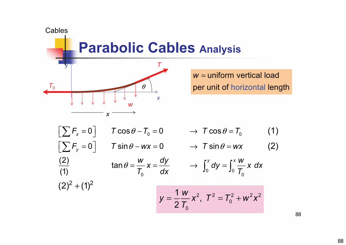
Parabolic Cables Analysisy T
uniform vertical load w =
x
T0
w
θ per horizon unit talof length
0 00 cos 0 cos (1)xF T T T Tθ θ = − = → =
x
0 sin 0 sin
(2) tan
(2)y
y x
F T wx T wx
w dy wx dy x dx
θ θ
θ
= − = → =
→
0 00 0
2 2
tan (1)
(2) (1)
x dy x dxT dx T
θ = = → =
+
1 w
88
2 2 2 2 20
0
1 , 2
wy x T T w xT
= = +
89
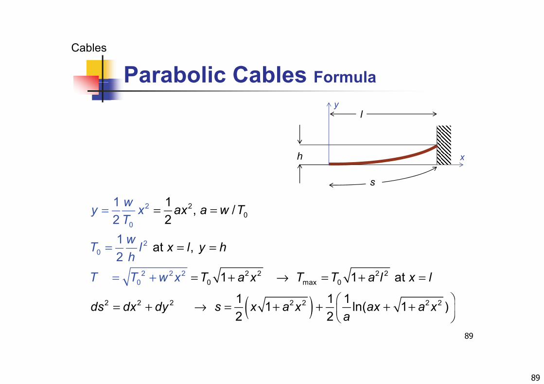
Parabolic Cables Formula
Cables
Parabolic Cables Formula
ly
h x
s
20
2 1 , /1 ax a w Twy x = == 00
20
, /2
at , 1 2
2ax a w T
x l y h
y xTwT lh
= ==
( )2 2 2 2
0 max 0
2 2
2 2 20
2 2 2 2 2
1 1 at
1 1 1 (
2
)
T a x T Th
T T a l x lw x = += + → = + =
89
( )2 2 2 2 2 2 21 1 11 ln( 1 )22
ds dx dy s x a x ax a xa
= + → = + + + +
90
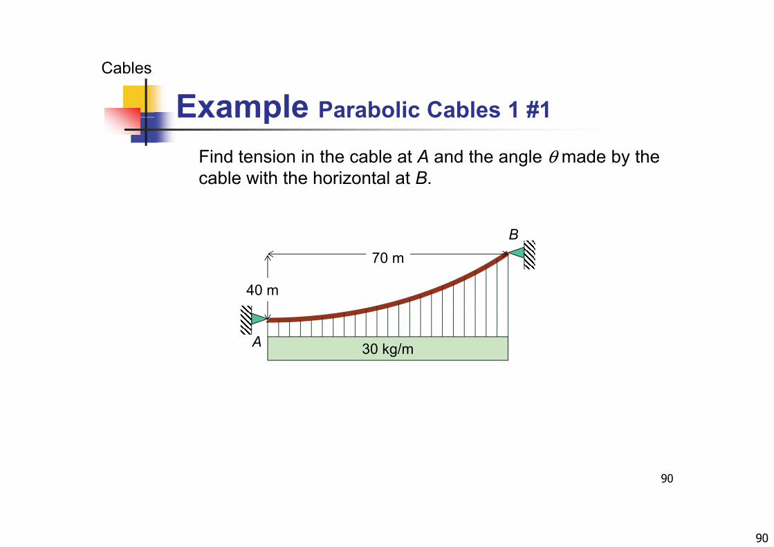
Example Parabolic Cables 1 #1
Cables
Example Parabolic Cables 1 #1
Find tension in the cable at A and the angle θ made by the cable with the horizontal at Bcable with the horizontal at B.
B70 m
40 m
30 kg/mA
90
91
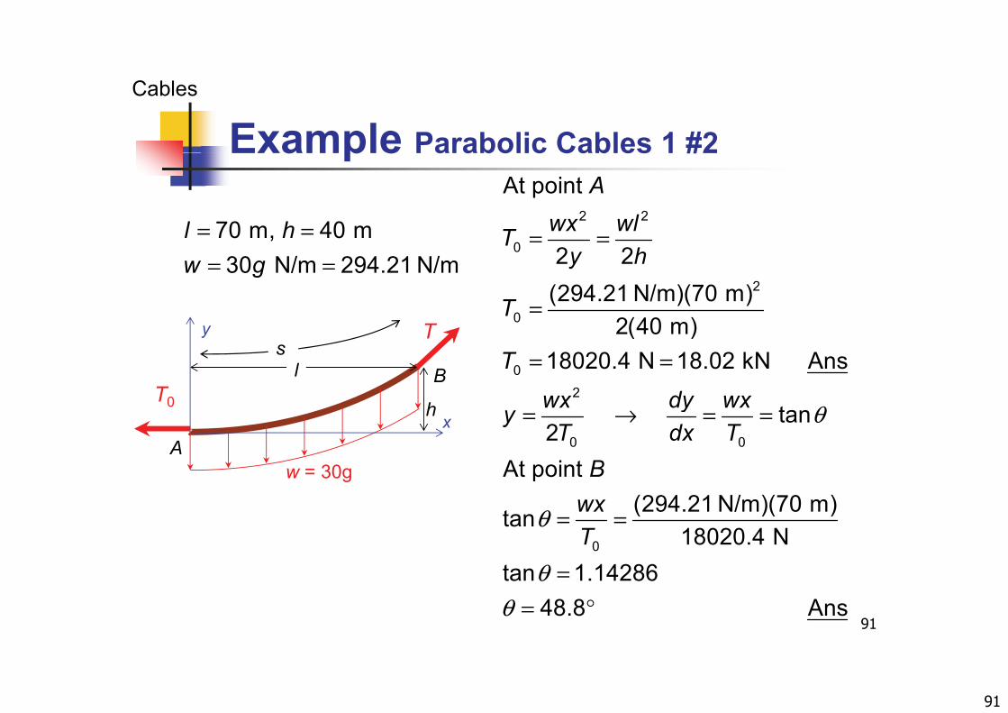
Example Parabolic Cables 1 #2
Cables
Example Parabolic Cables 1 #2
2 2
At point Awx wlT= =70 m 40 ml h = =
=
0
2
0
2 2(294.21 N/m)(70 m)
Ty h
T
= == =70 m, 40 m30 N/m 294.21 N/m
l hw g
= =
0
02
2(40 m)18020.4 N 18.02 kN Ans
T
T
wx dy wxl B
T
T0
sy
θ= → = =0 0
tan2
At point
wx dy wxyT dx T
B
h
A
T0
w = 30g
x
θ = =0
p(294.21 N/m)(70 m)tan
18020.4 NwxT
g
91
θθ
== °
tan 1.1428648.8 Ans
92
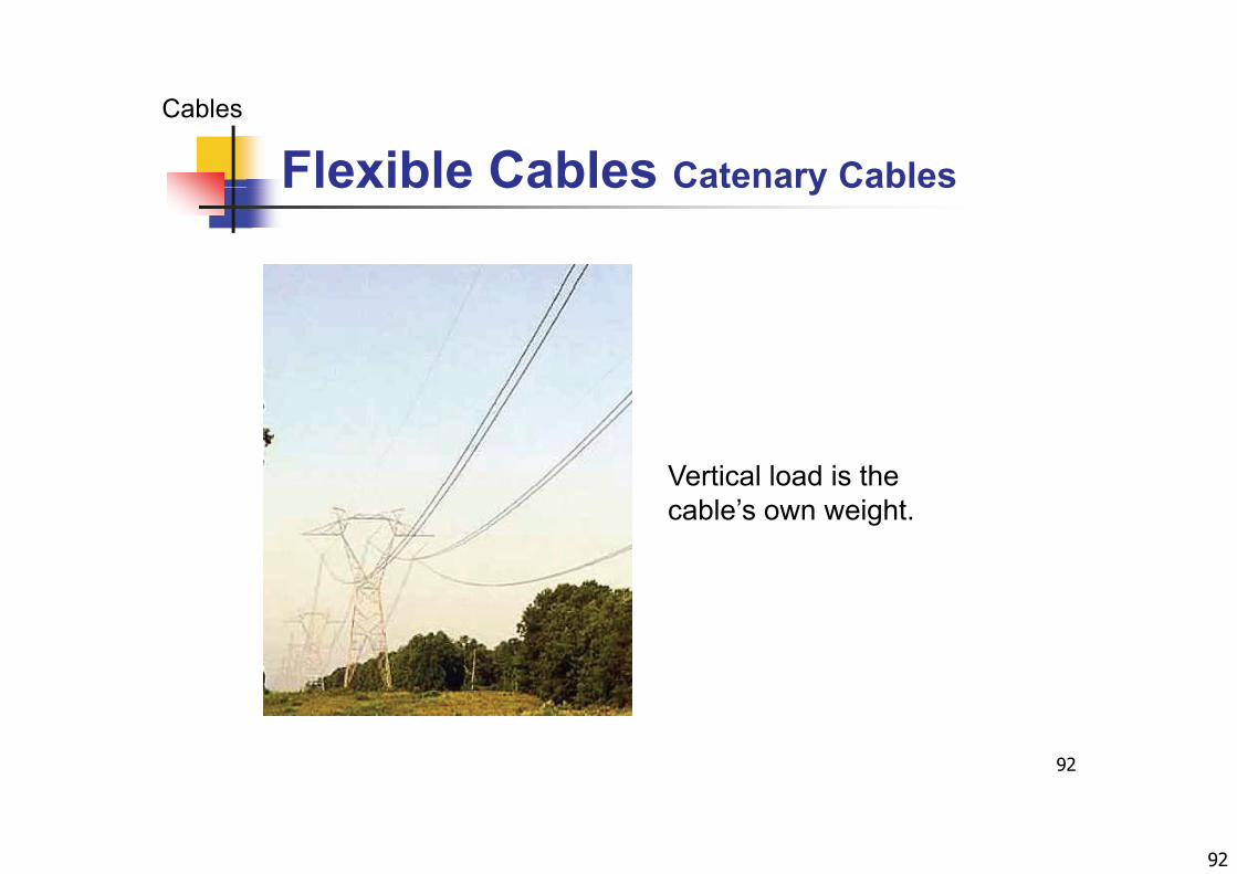
Flexible Cables Catenary Cables
Cables
Flexible Cables Catenary Cables
Vertical load is the cable’s own weight.
92
93
Catenary Cables Analysis #1
Cables
Catenary Cables Analysis #1
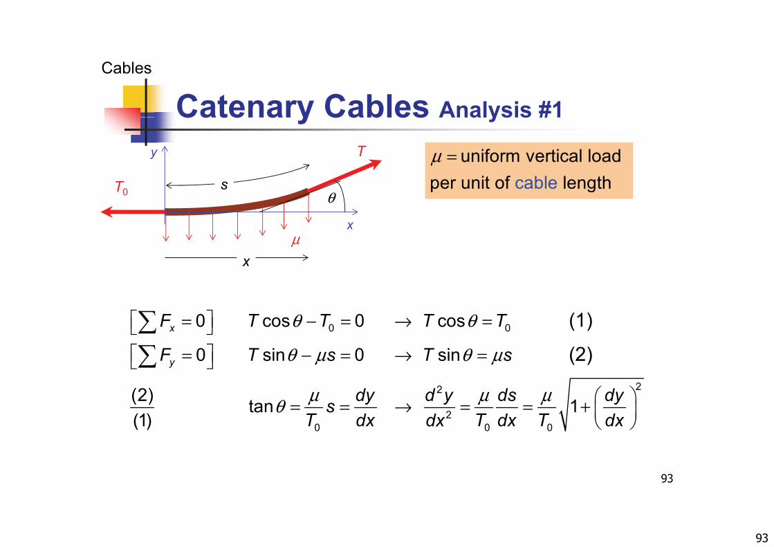
uniform vertical load per unit of cable lengthμ =Ty
per unit of cable lengthT0
μx
θs
xμ
0 00 cos 0 cos
0 sin 0 sin
(1)
(2)x
y
F T T T T
F T s T s
θ θ
θ μ θ μ
= − = → = = − = → =
22
20 0 0
(2) tan 1(1)
y
dy d y ds dysT dx T dx T dxdxμ μ μθ
= = → = = +
93
0 0 0( )
94
Catenary Cables Analysis #2
Cables
Catenary Cables Analysis #2
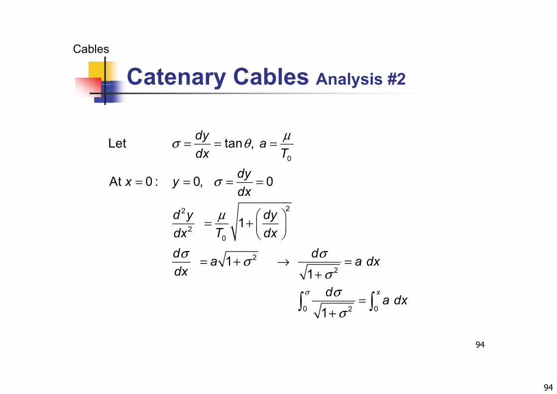
0
Let tan , dy adx T
dy
μσ θ= = =
22
At 0 : 0, 0
1
dyx ydx
d y dy
σ
μ
= = = =
2
0
2
1
1
y yT dxdx
d da a dx
μ
σ σσ
= +
= + → =2
0 02
1 1
1
x
a a dxdx
d a dxσ
σσ
σ
+ →+
=
94
0 021 σ+
95
Catenary Cables Formula
Cables
Catenary Cables Formula
ly
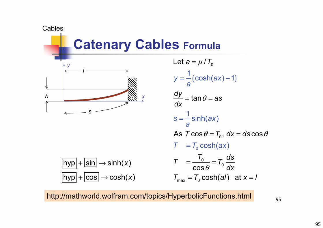
( )0Let /
1a Tμ=
h x
( )
tan
1 cosh( ) 1
dy as
y axa
θ
= −
= =
s 1 sinh( )
dx
s axa
=
0
0
As cos , coscosh( )
TT T
T dx dsxa
θ θ=
= =
00
0
coscosh( ) at
T dsT TdxlT T a x l
θ= =
= =
hyp sin sinh( )
hyp cos cosh( )
x
x
+ →
+ →
95
ax 0m cosh( ) at lT T a x lhyp cos cosh( )x+ →
http://mathworld.wolfram.com/topics/HyperbolicFunctions.html
96
Catenary Cables Hyperbolic Functions
Cables
Catenary Cables Hyperbolic Functions
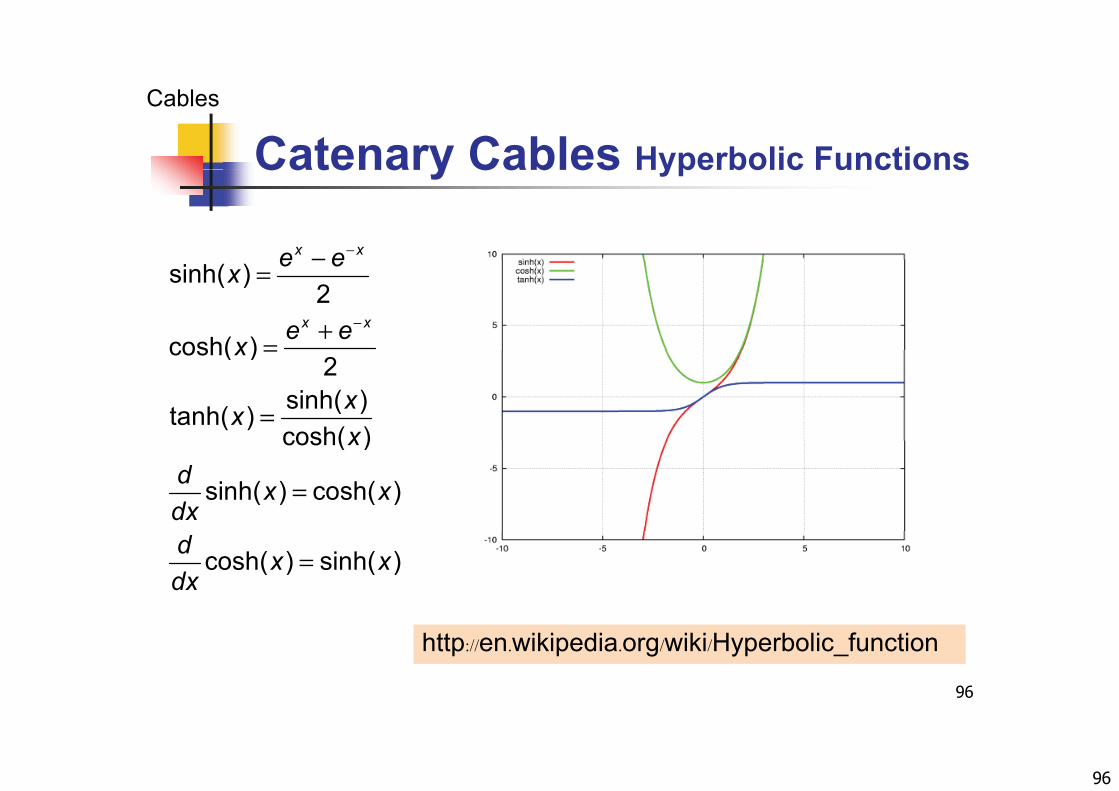
x xe e−−sinh( )2
cosh( )x x
e ex
e ex−
−=
+=cosh( )2
sinh( )tanh( )cosh( )
x
xxx
=
=cosh( )
sinh( ) cosh( )
xd x xdx
=
cosh( ) sinh( )d x xdx
=
96
http://en.wikipedia.org/wiki/Hyperbolic_function
97
Example Catenary Cables 1 #1
Cables
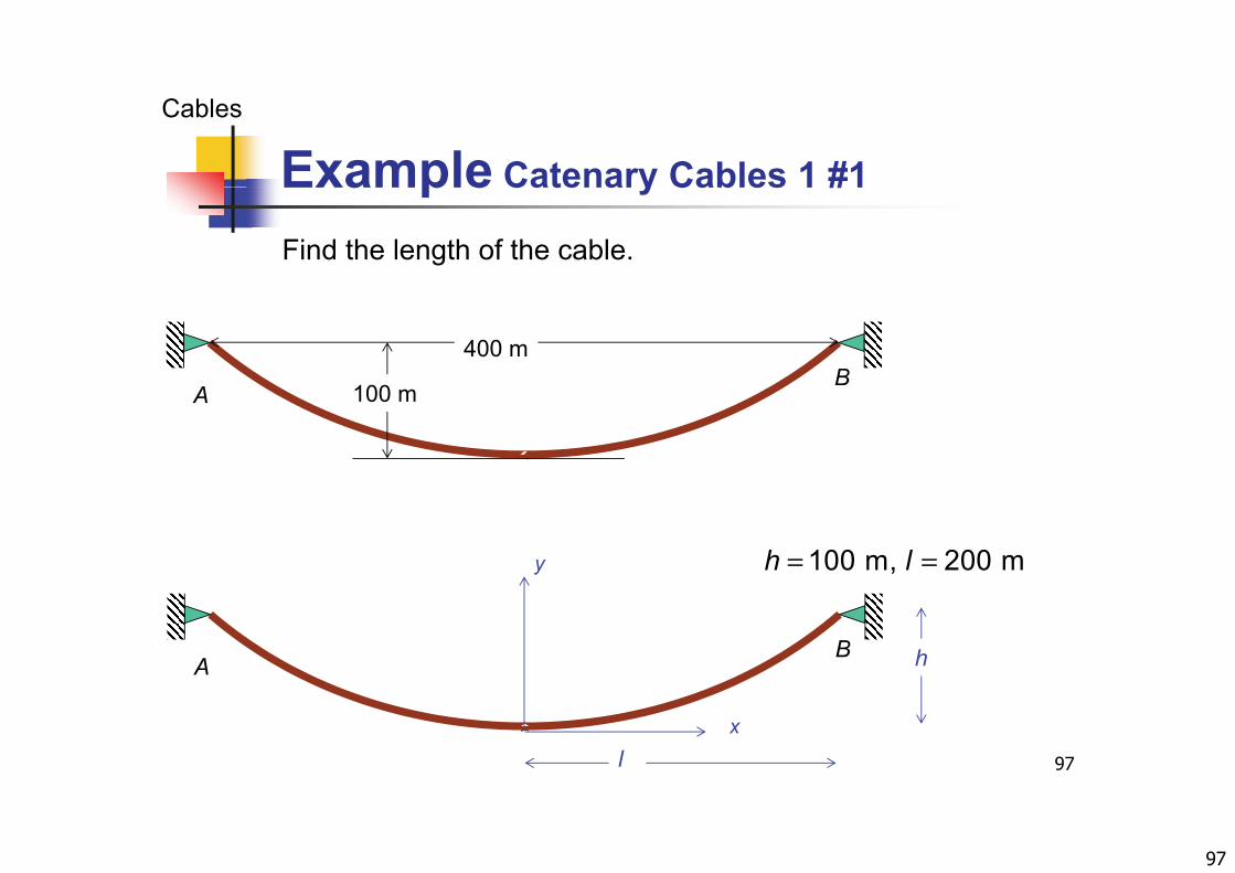
Example Catenary Cables 1 #1
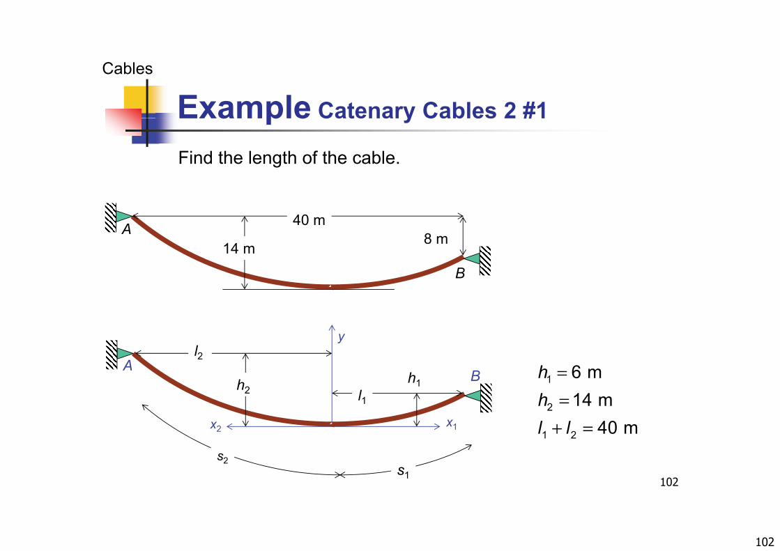
Find the length of the cable.
400 m
100AB
100 mA
y 100 m, 200 mh l= =
AB h
97
x
l
98
Example Catenary Cables 1 #2
Cables
Example Catenary Cables 1 #2
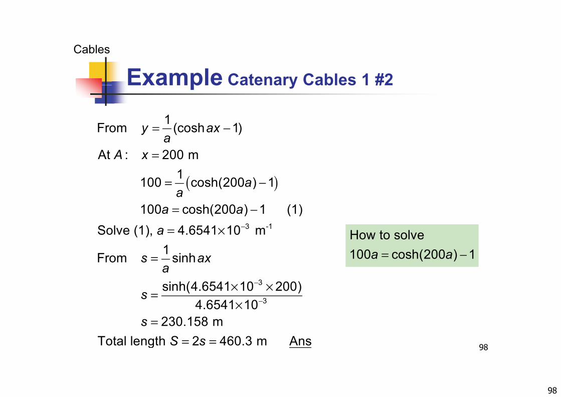
= −1From (cosh 1)y ax
=
From (cosh 1)
At : 200 m 1
y axa
A x
( )= −
= −
1100 cosh(200 ) 1
100 cosh(200 ) 1 (1)
aa
a a−= ×
=
3 -1Solve (1), 4.6541 10 m1From sinh
a
s axa
How to solve100 cosh(200 ) 1a a= −
−
−
× ×=×
3
3
sinh(4.6541 10 200) 4.6541 10
a
s
98
== =
230.158 mTotal length 2 460.3 m Ans
sS s
99
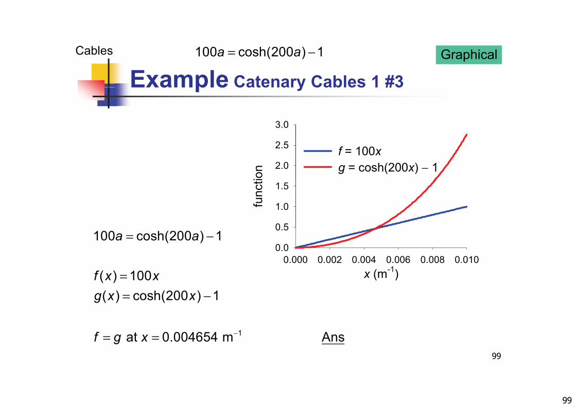
Example Catenary Cables 1 #3GraphicalCables = −100 cosh(200 ) 1a a
Example Catenary Cables 1 #3
3.0
ion 2.0
2.5 f = 100xg = cosh(200x) − 1
func
t
0 5
1.0
1.5
= −100 cosh(200 ) 1
( ) 100
a a
f x x x (m-1)0.000 0.002 0.004 0.006 0.008 0.010
0.0
0.5
== −
( ) 100( ) cosh(200 ) 1
f x xg x x
x (m )
99
−= = 1 at 0.004654 m Ansf g x
100
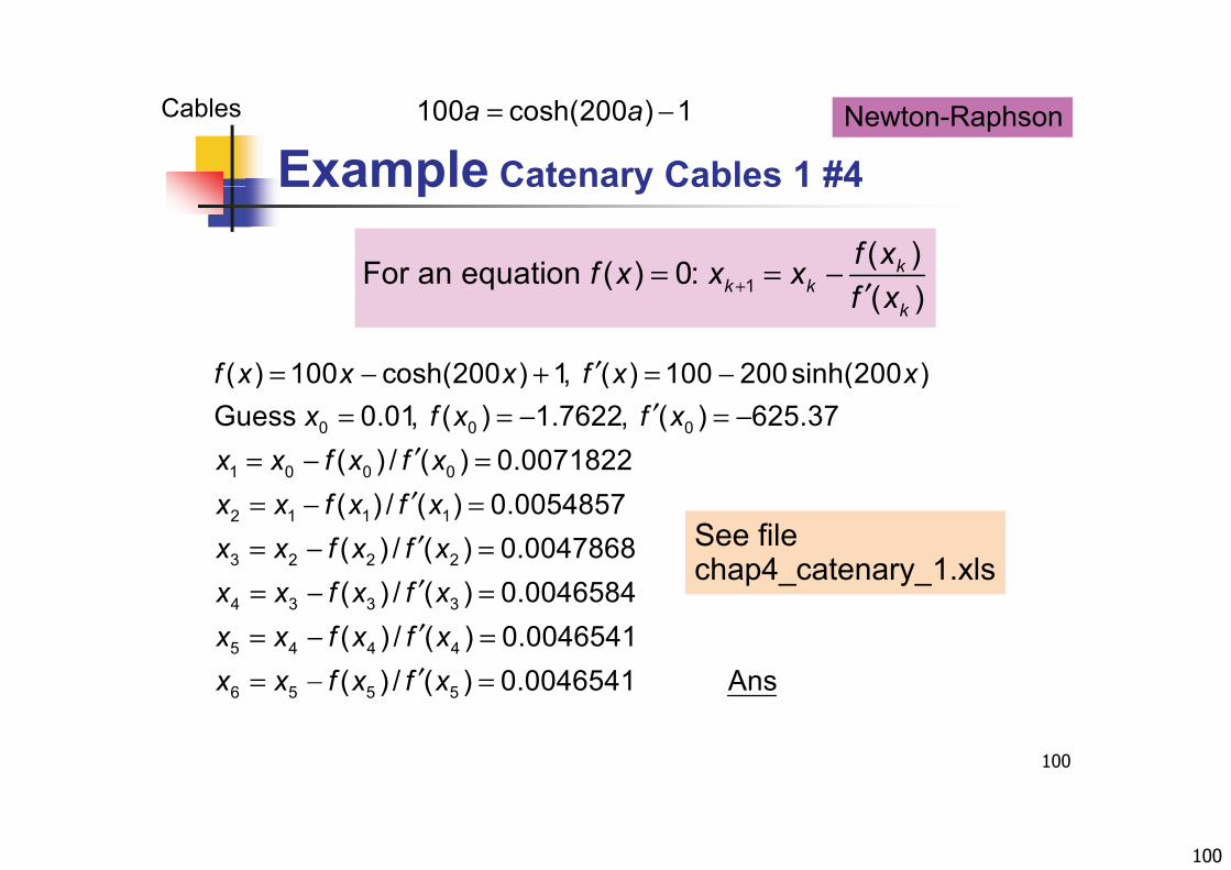
Example Catenary Cables 1 #4Newton-RaphsonCables = −100 cosh(200 ) 1a a
Example Catenary Cables 1 #4
1( )For an equation ( ) 0: ( )
kk k
f xf x x xf+= = −′1q ( )( )k k
kf x+ ′
′= − + = −( ) 100 cosh(200 ) 1, ( ) 100 200sinh(200 )f x x x f x x′= = − = −
′= − =0 0 0
1 0 0 0
( ) ( ) , ( ) ( )Guess 0.01, ( ) 1.7622, ( ) 625.37
( ) / ( ) 0.0071822x f x f x
x x f x f x′= − =′= − =′
2 1 1 1
3 2 2 2
( ) / ( ) 0.0054857( ) / ( ) 0.0047868( ) / ( ) 0 0046
x x f x f xx x f x f x
f f 584
See filechap4_catenary_1.xls
′= − =4 3 3 3( ) / ( ) 0.0046x x f x f x′= − =′= − =
5 4 4 4
584( ) / ( ) 0.0046541( ) / ( ) 0 0046541 Ans
x x f x f xx x f x f x
p _ y_
100
= =6 5 5 5( ) / ( ) 0.0046541 Ansx x f x f x

101
Example Catenary Cables 1 #5
Cables = −100 cosh(200 ) 1a a Newton-Raphson
Example Catenary Cables 1 #5
0 0
0.5
x0x1
f(x0)/f'(x0)
ctio
n f
-0.5
0.0 01
func
-1.5
-1.0 f = 100x
x (m-1)0.000 0.002 0.004 0.006 0.008 0.010
-2.0
101Numerical Methods in Engineering by Prof. Pramote Dechaumphai
102
Example Catenary Cables 2 #1
Cables
Example Catenary Cables 2 #1
Find the length of the cable.
40 m
14A 8 m14 m
B
6 mh
y
Al2
1
2
1 2
6 m14 m
40 m
hhl l
==
+ =x1x2
AB
l1h1h2
102
1 2 40 ml l+s2
s1
103
Example Catenary Cables 2 #2
Cables
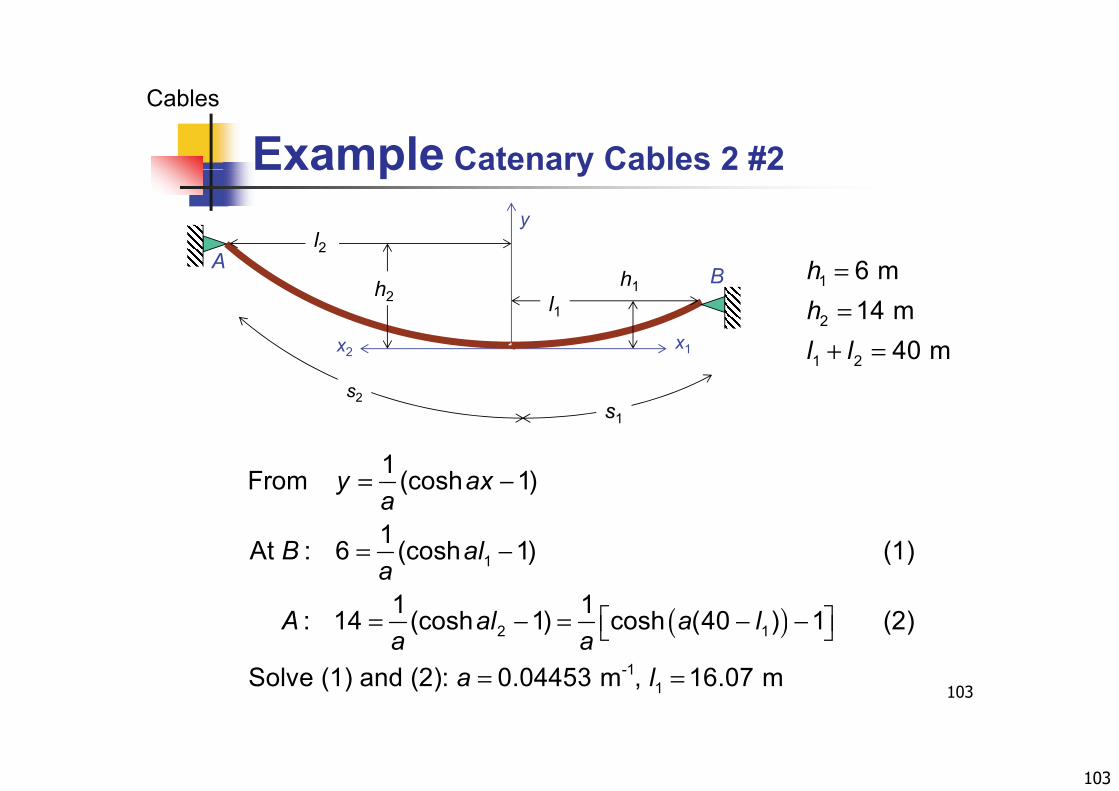
Example Catenary Cables 2 #2y
Al2
1
2
6 m14 m
40 m
hhl l
==
+ =x1x2
AB
l1h1h2
1 2 40 ml l+ =1x2
s2s1
1From (cosh 1)
1
y axa
= −
( )
11At : 6 (cosh 1) (1)
1 1: 14 (cosh 1) cosh (40 ) 1 (2)At
B ala
A al a l
= −
= =
103
( )2 1
-11
: 14 (cosh 1) cosh (40 ) 1 (2)
Solve (1) and (2): 0.04453 m , 16.07 m
At A al a la a
a l
= − = − −
= =

104
Example Catenary Cables 2 #3
Cables
Example Catenary Cables 2 #3y
Al2
1
2
6 m14 m
40 m
hhl l
==
+ =x1x2
AB
l1h1h2
1 i h
1 2 40 ml l+ =1x2
s2s1
=
= × =1
1 sinh
1 sinh(0.04453 16.07) 17.477 m
s axa
s
( )
×
= − =
1
2
sinh(0.04453 16.07) 17.477 m0.04453
1 sinh 0.04453(40 16.07) 28.723 m0.04453
s
s
104= + =1 2
0.04453
Total cable length 46.2 m AnsS s s
105
Example Catenary Cables 2 #4
Cables Newton-Raphson
Example Catenary Cables 2 #4
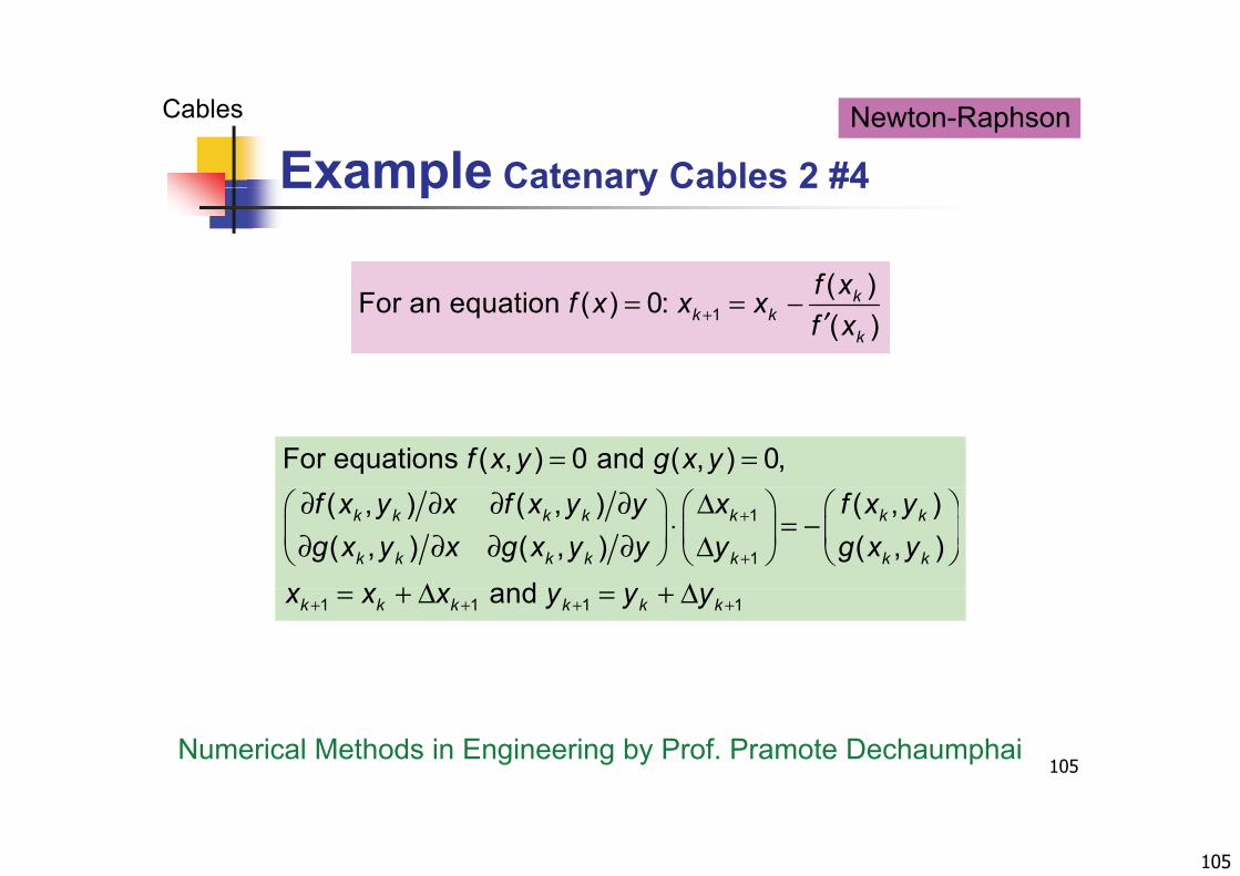
( )f x1
( )For an equation ( ) 0: ( )
kk k
k
f xf x x xf x+= = −′
For equations ( , ) 0 and ( , ) 0,f x y g x y= =
1
1
( , ) ( , ) ( , )( , ) ( , ) ( , )
and
k k k k k k k
k k k k k k k
f x y x f x y y x f x yg x y x g x y y y g x y
x x x y y y
+
+
∂ ∂ ∂ ∂ Δ ⋅ = − ∂ ∂ ∂ ∂ Δ
+ Δ + Δ1 1 1 1and k k k k k kx x x y y y+ + + += + Δ = + Δ
105Numerical Methods in Engineering by Prof. Pramote Dechaumphai
106
Example Catenary Cables 2 #5
Cables Newton-Raphson
Example Catenary Cables 2 #5
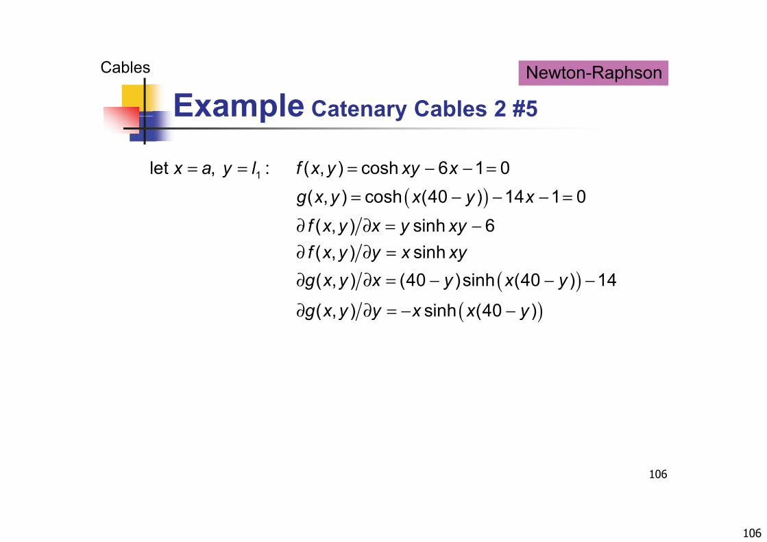
1let , : ( , ) cosh 6 1 0x a y l f x y xy x= = = − − =
( )1
( , ) cosh (40 ) 14 1 0( , ) sinh 6
g x y x y xf x y x y xy
= − − − =
∂ ∂ = −
( )( )
( , ) sinh( , ) (40 )sinh (40 ) 14
f x y y x xyg x y x y x y
∂ ∂ =∂ ∂ = − − −
( )( , ) sinh (40 )g x y y x x y∂ ∂ = − −
106
107
Example Catenary Cables 2 #7
Cables Newton-Raphson
Example Catenary Cables 2 #7
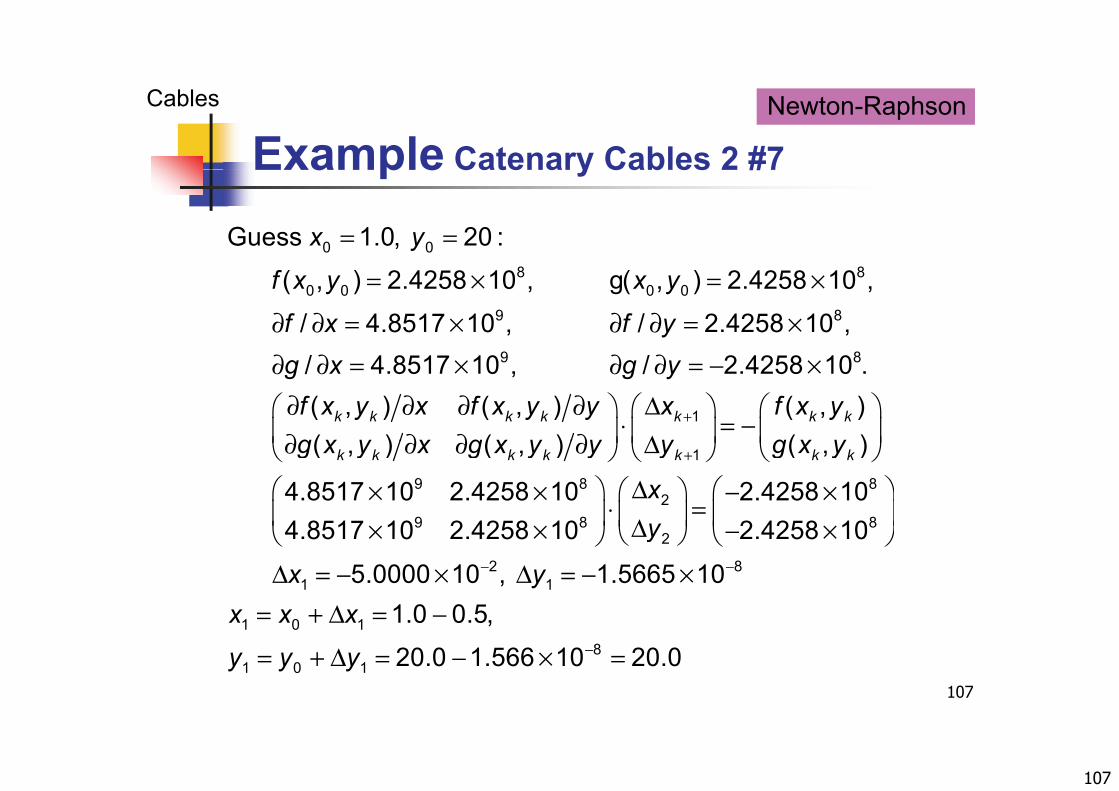
= =0 0Guess 1.0, 20 :x y
= × = ×
∂ ∂ = × ∂ ∂ = ×
8 80 0 0 0
9 8
( , ) 2.4258 10 , g( , ) 2.4258 10 ,
/ 4.8517 10 , / 2.4258 10 ,
f x y x y
f x f y
+
∂ ∂ = × ∂ ∂ = − ×∂ ∂ ∂ ∂ Δ
⋅ = ∂ ∂ ∂ ∂ Δ
9 8
1
/ 4.8517 10 , / 2.4258 10 .( , ) ( , )( ) ( )
k k k k k
g x g yf x y x f x y y xg x y x g x y y y
−
( , )( )
k kf x yg x y+
∂ ∂ ∂ ∂ Δ 1( , ) ( , )k k k k kg x y x g x y y y
Δ × × − ×⋅ = Δ× × ×
9 8 82
9 8 8
( , )
4.8517 10 2.4258 10 2.4258 104 8517 10 2 4258 10 2 4258 10
k kg x y
xy
− −
Δ× × − × Δ = − × Δ = − ×
= + Δ = −
2
2 81 1
1 0 1
4.8517 10 2.4258 10 2.4258 10
5.0000 10 , 1.5665 101.0 0.5,
y
x yx x x
107
−
+ Δ
= + Δ = − × =1 0 1
81 0 1
1.0 0.5,
20.0 1.566 10 20.0
x x x
y y y
108
Example Catenary Cables 2 #8
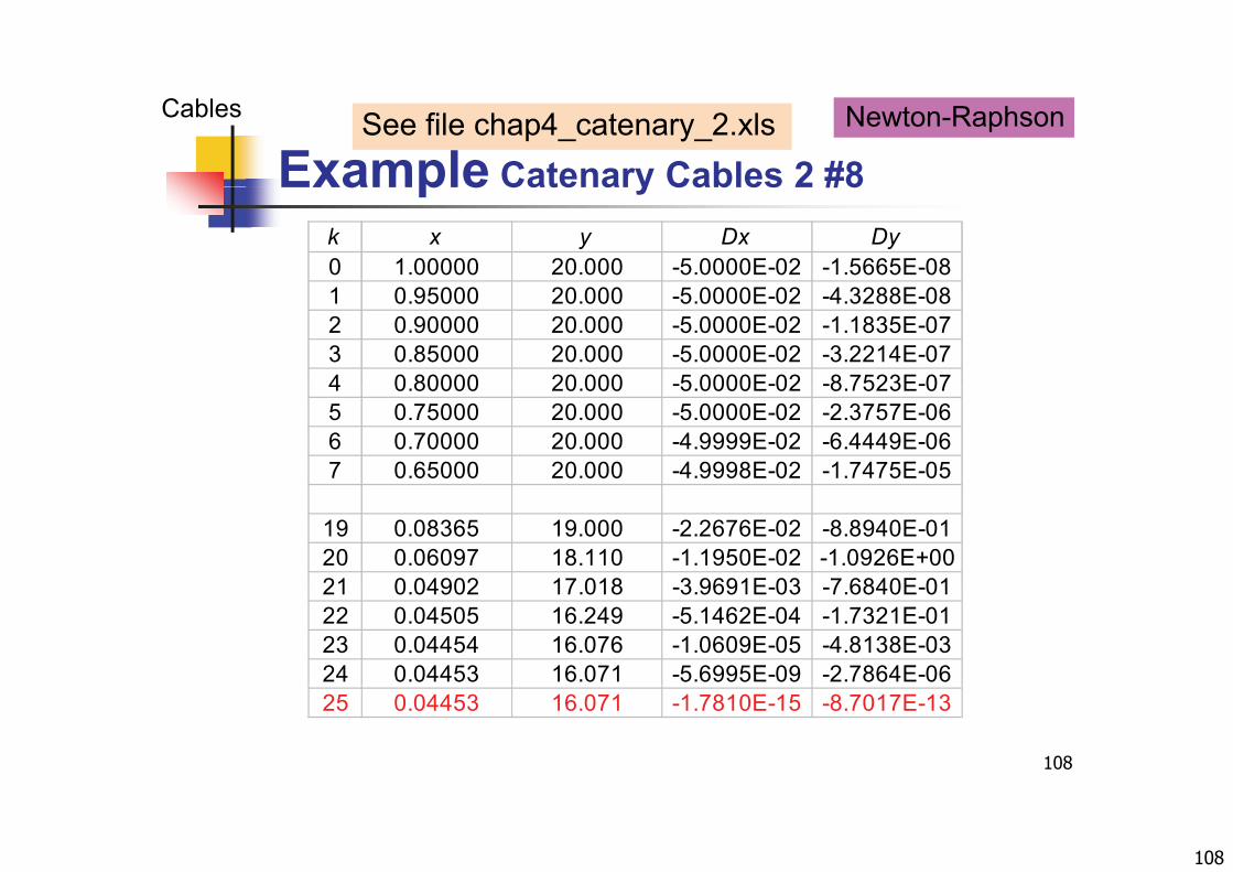
Cables Newton-RaphsonSee file chap4_catenary_2.xls
Example Catenary Cables 2 #8k x y Dx Dy0 1.00000 20.000 -5.0000E-02 -1.5665E-081 0.95000 20.000 -5.0000E-02 -4.3288E-082 0.90000 20.000 -5.0000E-02 -1.1835E-073 0.85000 20.000 -5.0000E-02 -3.2214E-074 0 80000 20 000 -5 0000E-02 -8 7523E-074 0.80000 20.000 5.0000E 02 8.7523E 075 0.75000 20.000 -5.0000E-02 -2.3757E-066 0.70000 20.000 -4.9999E-02 -6.4449E-067 0.65000 20.000 -4.9998E-02 -1.7475E-05
19 0.08365 19.000 -2.2676E-02 -8.8940E-0120 0.06097 18.110 -1.1950E-02 -1.0926E+0021 0 04902 17 018 3 9691E 03 7 6840E 0121 0.04902 17.018 -3.9691E-03 -7.6840E-0122 0.04505 16.249 -5.1462E-04 -1.7321E-0123 0.04454 16.076 -1.0609E-05 -4.8138E-0324 0.04453 16.071 -5.6995E-09 -2.7864E-06
108
25 0.04453 16.071 -1.7810E-15 -8.7017E-13
109
Concepts #1
Review
Concepts #1
Centroid, center of mass and center of gravityrespectively represent the centers of geometry massrespectively represent the centers of geometry, massand weight.
Pappus theorems can be used to find the surface area and volume of revolutions.
Apart from moments of forces, there are several kinds of moments. The first moment of area is a property of cross section that is used to predict its resistance to shearsection that is used to predict its resistance to shear stress. The moment of inertia quantifies the rotational inertia of a body. The polar moment of inertia is a property of cross section that is used to predict its
109
property of cross section that is used to predict its resistance to torsion.
110
Concepts #2
Review
p The equivalent resultant of the distributed loads can be used
in the analyses instead of the distributed loads The area andin the analyses instead of the distributed loads. The area and volume analogies help visualized the line and surface distributed loads on bodies.Th fl id t ti d l ith th ff t f fl id t t The fluid statics deal with the effects of fluid at rest. The pressure, exerted by the fluid in the perpendicular
direction with respect to the surface in contact with the fluid, varies linearly with depth.
The block of fluid is an addition method to determine resultants.resultants.
Flexible cables can support tension only. Parabolic cables are loaded with uniform force per unit
l th
110
span length. Catenary cables are loaded with uniform force per unit of
cable length.