3dof estimation of agile space objects using marginalized ...rlinares/papers/2017_02.pdf · 3dof...

3DOF Estimation of Agile Space Objects usingMarginalized Particle Filters

Ryan D. Coder* and Marcus J. Holzinger†

Georgia Institute of Technology, Atlanta, GA, 30332

Richard Linares‡

University of Minnesota, Minneapolis, MN, 55455

Several innovations are introduced to ameliorate error in light curve based space object atti-

tude estimation. A radiometric measurement noise model is developed to define the observation

uncertainty in terms of optical, environmental, space object, and sensor parameters and is vali-

dated using experimental data. Additionally, a correlated angular acceleration dynamics model is

adopted to model the unknown inertia and body torques of agile space objects. This linear dynam-

ics model enables the implementation of marginalized particle filters, affording computationally

tractable 3 degree of freedom Bayesian estimation. The synthesis of these novel approaches en-

able the estimation of attitude and angular velocity states of maneuvering space objects without a

priori knowledge of initial attitude, while maintaining computational tractability. Simulated results

are presented for the full 3 degree of freedom agile space object attitude estimation problem.

I. Introduction

Improvements in Space Domain Awareness (SDA) are identified in multiple national policy doc-

uments as a top priority to protect the US and its allies as well as maintain its economic and

diplomatic objectives [1]. The high level activities of SDA include the detection, tracking, char-

acterization, and analysis of space objects (SOs), as defined in Joint Publication 3-14, “Space

Operations” [2]. Space objects are typically defined as active and inactive satellites, rocket bodies,

and orbital debris [3]. To fully characterize space objects, it is necessary to obtain knowledge about

*Ph.D. Candidate, Guggenheim School of Aerospace Engineering, [email protected]†Asst. Professor, Guggenheim School of Aerospace Engineering, [email protected], AIAA Senior Member‡Asst. Professor, Aerospace Engineering and Mechanics, [email protected], AIAA Member

1 of 35

American Institute of Aeronautics and Astronautics

both SO shape and attitude, which can inform SO payload capability or mission purpose [4]. For

SOs in low Earth orbit, shape and attitude estimation is performed extensively using radar-based

methods pioneered in the early 1980s [5]. The shape and attitude of large SOs can also be esti-

mated from resolved imagery taken by ground based optical sensors. However, when SOs are too

distant to be imaged by radar facilities or too small to be adequately resolved by ground based

optical sensors, the primary source of data processed is unresolved imagery [4].

Each unresolved image can be analyzed to determine the power reflected by the SO. A typical

observation campaign of several images can then be used to create a light curve: a temporally

resolved sequence of power measured over specified wavelengths. Because the total amount of

flux reflected by the SO is dependent on the SO shape and attitude, estimating either the attitude

or shape of the SO is possible using the observed light curve [6]. This process is referred to

as light curve inversion, and was initially developed to characterize asteroids [7]. Past efforts to

characterize asteroids have used batch estimation methods, where attitude, angular rates, moments

of inertia and shape model are all simultaneously estimated [8–11].

While the light curve inversion process is similar, there are several important differences be-

tween asteroids and man-made SOs. The first significant difference is that unlike asteroids, many

SOs have highly angular surfaces composed of several materials. Consequently, the estimated SO

attitude is often separated from materials and shape properties, collectively referred to as the SO

“shape model” [4]. Another difference is that active satellites employ actuators to change and

maintain mission specific orientations, requiring dynamics models which account for this motion

without knowledge of the external torques or inertia tensor of the satellite.

The first work outlining the theoretical application of light curve inversion to SO character-

ization was given by Hall et al. in 2005 [6]. The first study to provide simulated results for

non-maneuvering SOs utilizes a single Unscented Kalman Filter (UKF) to estimate either the SO

attitude, shape model, or both simultaneously. The synthetically generated measurements are cor-

rupted by time-invariant, zero mean Gaussian white noise whose covariance is represented in the

visual magnitude scale based on historical observations. The authors of that work concluded that

more accurate measurement models could alleviate discrepancies between observational and sim-

2 of 35


ulated data [12]. To mitigate these issues, recent work by the first author can be expanded upon to

define a radiometric measurement noise model, based on SO and environmental parameters [13].

This first contribution increases the likelihood that estimators that work well in simulation will also

perform well with operational data.

More recent SO attitude estimation effort have recognized that bidirectional reflectivity distri-

bution function (BRDF) measurement models are non-linear functions of attitude states, resulting

in potentially non-Gaussian state distributions. Recognizing the limitations of UKFs for distribu-

tions not accurately summarized by a mean and variance, this past effort utilizes a particle filter

(PF) to estimate the attitude states of agile SOs. It is also shown how shape model bias can be in-

cluded in the estimated states. The simulated results presented utilize a visual magnitude measure-

ment noise based on historically collected measurement data, like work before it. To account for

the unknown SO torques and inertia properties, SO angular rates are modeled as a white noise pro-

cess. The number of particles necessary for this approach presents a computational challenge [14].

To reduce the number of particles required using this brute force model, a more sophisticated

dynamics model is proposed in this investigation. Many tracking methods have addressed the prob-

lem of unknown motion by assuming that the unknown acceleration can be modeled as a Markov

process, where the acceleration is correlated exponentially over short periods of time [15–19].

Thus, the second contribution of this work is to adapt this idea, such that SO angular accelera-

tions are correlated exponentially over short periods of time. This exponentially correlated model

makes the body angular velocities continuous with time, as they are in true kinematic motion. This

continuity is not reflected in the previous white noise model.

Defining the attitude, attitude rates, and attitude accelerations for 3 degrees of freedom (3DOF)

motion requires a minimum of 9 states. Including bias terms for shape uncertainty increases the

dimensionality. Since particle filters computation scales exponentially with state space dimension,

estimating large numbers of states is computational intractable. To ameliorate this curse of dimen-

sionality, the final contribution of this work is to apply marginalized particle filters (MPFs), also

known as a Rao-Blackwellized filters [20]. The core concept of the marginalized particle filter is to

exploit any linear sub-structure in the model that is subject to Gaussian noise [21]. Because the ex-

3 of 35


ponentially correlated dynamics model proposed are described by a linear set of equations, MPFs

reduce the number of nonlinear states to 3. Critically, this enables the estimation of attitude and

angular velocity states of maneuvering space objects without a priori knowledge of initial attitude,

while maintaining computational tractability.

This work is organized as follows. The first contribution of this work, the radiometric mea-

surement noise model, is presented in the Measurement Noise Model subsection. The second

contribution, the exponentially correlated angular acceleration dynamics model, is presented in

the Exponentially Correlated Angular Acceleration Model subsection. The third contribution is

presented in the Marginalized Particle Filter subsection. A simulation framework, results, and

discussion are presented in the Simulated Results section.

II. Radiometric and Electro-Optical Sensor

Developing a radiometric measurement noise model requires two elements. The first is an accurate

accounting of the number of photons emitted by the Sun, reflected off the SO, and ultimately

captured in the EO sensor of a telescope. This first part is covered in this subsection A. The second

is a description of how these photons are recorded by an electro-optical sensor, and how much noise

is added to the total SO signal by the sensor itself. This second portion is covered in subsection B.

A. Space Object Signatures

By convention, SO brightness is quantified using the apparent visual magnitude system, first de-

veloped by early astronomers. The system is unitless, logarithmic, and references the brightness

of Vega as the scale’s zero point. The resulting SO signature represented in the apparent visual

magnitude system, mv,SO, is found using Eq. (1) [22].

mv,SO = mv,Sun � 2.5 log10

MSO

MSun

!(1)

4 of 35


The visual magnitude of the Sun is typically given as -26.73 and MSO is the total radiant excitance

of the SO, which is given by Eq. (2).

MSO =1R2

Z �UL

�LL

MSun (�) Fr

⇣✓B

I , s, R, �⌘

d� (2)

In this equation, R is the distance from the SO to the observer, MSun (�) is the spectral excitance

of the Sun at the Earth integrated between the wavelength limits �LL and �UL, and Fr is the bidi-

rectional reflectivity distribution function (BRDF). The BRDF determines the number of photons

reflected from the SO towards the observer and is a function of shape model, material composition,

and SO attitude. The quantity s is the unit vector from the Sun to the SO and the rotation from

the inertial frame to the body frame of the SO is denoted by ✓BI . The spectral excitance of the

Sun can be modeled using a black-body radiator assumption [22]. The solar spectral excitance is

then converted to a photon flux density, �SO, in photons/s/m2, assuming a weighted average for

the wavelengths of light reflected. The light gathering capabilities of a ground-based sensing ap-

plication can then be calculated as the photon flux captured by the optical system, qSO, measured

in e�/s, is given by Eq. (3) [23].

qSO = �SO⌧atm⌧opt

⇡D2

4

!QE (3)

In Eq. (3), the aperture diameter of the telescope is D, while ⌧atm and ⌧opt are the transmittance

of the atmosphere and optics assembly respectively. The quantum efficiency of the EO sensor is

defined as QE. The value of these two transmittances and the QE are wavelength dependent. In lieu

of more detailed modeling, these three variables are defined to have values ranging from ⌧ 2 (0, 1]

and QE 2 (0, 1] using a weighted average value for the wavelength of incident light.

To accurately characterize noise due to background light, the local background radiant inten-

sity, Isky, whose major sources are moonlight and local light pollution, must be determined. In

relatively light polluted areas, it is suggested that a sky sensor is utilized to directly measure this

quantity. Typical values for radiant intensity vary from Isky 2 [15, 22] mv/arcsec2 for urban and

rural skies respectively. The total photon radiance at the telescope aperture due to background sky

5 of 35


pollution, Lsky, in photons/s/m2/sr, is given by Eq. (4) [23].

Lsky = �010�0.4Isky

180⇡

!2

36002 (4)

Here, the variable �0 is the radiant intensity of the reference zero point, which traditionally is

the star Vega. A final expression for the photon flux per pixel resulting from background radiant

intensity, qp,sky, is expressed in e�/s/pixel as shown in Eq. (5). The total incidence on the focal plane

transmitted from the radiance at the telescope aperture is found using the “camera equation” [24].

This work utilizes the simplified form of the camera equation for a singlet lens, valid for all focal

ratios, N, yielding the photon flux incident on the EO sensor in Eq. (5).

qp,sky =Lsky⌧opt⇡QEp2

1 + 4N2 (5)

In Eq. (5), the EO sensor is assumed to have square pixels. For non-square pixels, p2 can be

replaced by the appropriate pixel unit of area.

The radiometric model presented here is a summary of previous work, and additional details

are available to the interested reader [13]. The model defines the photon flux of SOs, in Eq. (3),

and the background sky brightness, in Eq. (5), as a function of various environmental variables and

optics system parameters. Using these two quantities, it is then possible to define both the mean

signal and variance from important noise sources in terms of electrons. These equations are valid

for EO sensors capturing unresolved images of SOs.

B. Noise Sources in EO Sensors

An excellent discussion on EO sensor noise sources, which includes the development the “CCD

Equation” and outlines a computer simulation of CCD noise, is presented by Merline and Howell

[25]. The goal of this subsection is to summarize the largest noise sources outlined in that work and

mathematically relate them to the equations of subsection A. Typically, the largest types of noise

inherent in unresolved images of SOs are Poisson or “shot” noise from the SO and background

radiant sky intensity, i.e. light pollution. To quantify the largest noise sources, let the total variance

6 of 35


in the integrated signal be defined as Eq. (6) [25].

�2S = m

✓1 +

mz

◆�2

r +

mX

i=1

⇥�Ci �C�i

�G⇤+

m2

z2

zX

j=1

h⇣C j �C�j

⌘Gi

(6)

In Eq. (6), the first term is due to readout noise, �2r , the second term is the photon noise of the

SO, and the third term is the photon noise from the background. This work neglects the variance

due to the conversion from electronics to analog-to-digital units (ADU), as well as the variance

in digitization offset, as these are less significant contributors. Furthermore, this derivation has

assumed that the variance of the total signal and background are uncorrelated and zero mean.It

is emphasized that Eq. (6) is written in units of electrons and not analog-to-digital units (ADU),

which are commonly referred to as “counts.” Therefore, the variance in a SO measurement is

calculated from the total counts, C, converted to electrons by the CCD gain, G. The superscript �

in the second and third terms indicates that these counts are due to direct current bias.

To relate these noise components to their physical sources, one must make assumptions about

the type and application of data reduction techniques. In this work, it is assumed that dark frame

subtraction and flat field corrections do not introduce additional sources of error. Therefore, the

subtraction of the direct current bias in Eq. (6) can be approximated as shown in Eq. (7) and Eq. (8),

thus linking the noise in collected images with their physical origins [25].

mX

i=1

⇥�Ci �C�i

�G⇤ ' qSOtI + m

⇣qp,sky + qp,dark

⌘(7)

zX

j=1

h⇣C j �C�j

⌘Gi' z

⇣qp,sky + qp,dark

⌘(8)

In Eq. (7) and Eq. (8), qSO is the photon flux reflected by the SO as defined in Eq. (3), qp,sky

is the photon flux per pixel from the background sky irradiance as defined in Eq. (5), and qp,dark

is the dark current per pixel. Additionally, tI is the integration time, i.e. exposure time, of the

observation. To accurately calculate the signal received by the sensor, one must subtract out the

background signal present. While many methods are available, this work assumes the simplest

7 of 35


technique which estimates the mean background signal from pixels which are free of stars, SOs,

and other objects of interest [26]. The subscript j is used to denote this random sample of z object-

free pixels used to determine the mean background noise, while the subscript i is used to denote a

pixel which lies in the array of pixels containing the SO, m. The arrival process of photons incident

on the CCD plane is described by a Poisson process. Consequently, the variance in the number of

electrons generated in an EO sensor can be defined by Eq. (9), by combining Eqs. (7 and 8) [27].

�2S ⇡ qS OtI + m

✓1 +

mz

◆ h⇣qp,sky + qp,dark

⌘tI + �

2r

i(9)

Eq. (9) shows how the noise present in images can be rudimentarily modeled. Critically, this model

assumes that the atmospheric transmittance, ⌧atm, is constant. Using the foundational knowledge

of this section, Section III.A demonstrates how one can model the atmospheric transmittance as a

random variable and how this increases the measurement variance.

III. Methodology

Using the brief summary of radiometry and EO noise literature of the previous section, a radio-

metric noise model in subsection A. Following this, subsection B summarizes the how the true

dynamics of an agile SO can be modeled with exponentially correlated angular accelerations, i.e.

the Singer model. Finally, subsection C details how the proposed dynamics model greatly reduces

computational burden when coupled with a marginalized particle filter.

A. Measurement Noise Model

The radiometric measurement function proposed in this section defines the noise present in an im-

age as a function of optical and environmental parameters. This stands in contrast to previous light

curve inversion studies for estimating satellite attitude, which use visual magnitudes and a time

invariant measurement variance [12, 14, 28]. It should be noted that these previous studies, which

implemented various sequential filters, could also implement the measurement model proposed in

this work. Because the number of photons incident on an EO sensor are typically on the order of

103 and higher, this Poisson process is well approximated by a Gaussian distribution, leading to

8 of 35


the definition of measurement noise in Eq. (11).

yk(x, tk) = qSO(x, tk) + vk(x, tk) (10)

vk(x, tk) ⇠ N (0,Rk(x, tk)) (11)

In Section II, the variance of a SO signature captured by an EO sensor is defined by Eq. (9).

In this equation, the values of atmospheric losses and sky brightness are deterministic. However,

the phase and position of the moon, time of night, presence of clouds, and scintillation effects all

cause the atmospheric transmittance and radiant sky intensity to be random variables. Atmospheric

transmittance and radiant sky intensity vary temporally and spatially, and both typically increase

near the local horizon. Since this work simulates the SO light curve over a short time period,

the radiant sky intensity is treated as constant while the atmospheric transmittance is treated as a

random variable. Depending on the power of the scintillation, for stars near the zenith atmospheric

transmittance is best described as a Gaussian, log-normal, or F distribution [29]. For simplicity of

implementation, this work will implement the atmospheric transmittance as a Gaussian distributed

random variable.

Consequently, this work proposes a mixed Poisson distribution for the measurement model. In

general, two elements are necessary to describe a mixture distribution: the conditional distribution

of a random variable on another and the distribution of the mixing parameter itself. Thus, the

number of photons incident on the EO sensor, ⇣, is a mixed Poisson random variable whose rate

parameter, �, is conditional on the normally distributed random mixing parameter, the atmospheric

transmittance. This can be written mathematically as shown in Eq. (12) [30].

⇣ ⇠ P(�)^

�

N(µatm,�atm) (12)

As is standard, � defines the typical number of photons per predefined interval. In Eq. (3), the

number of photons per second, qSO is defined. Thus, � = qSOtI , where tI is the length in seconds

of the image exposure. To define the measurement uncertainty, one need define the variance of the

9 of 35


mixed Poisson process. The variance of a mixed Poisson process has been analytically derived to

be greater than that of a homogenous Poisson process, as shown in Eq. (13) [31–33].

Var(⇣) = E[⇣2] � (E[⇣])2 = E[�] + Var(�) (13)

Here the expected value of the random variables is denoted using the standard notation, E[·]. To

evaluate the mean and variance of the rate parameter, note that the only random variable in Eq. (3)

is the atmospheric transmittance. Since it has been assumed in this work that the atmospheric

transmittance may be represented as a Gaussian random variable, and hence has finite first and

second moments, the mean and variance of the shot noise can be expressed as

E(�) = �SO⌧opt

⇡D2

4

!QE tI

!µatm (14)

Var(�) = �SO⌧opt

⇡D2

4

!QE tI

!2

�2atm (15)

One can define a time dependent zero mean Gaussian white noise using the covariance defined by

Eq. (16). Comparing the deterministic noise of Eq. (9) to Eq. (16) reveals that the only difference

is the addition of the second term in Eq. (16), which includes the effect of the varying atmosphere

Eq. (16)

Rk(x, tI) ⇡ E(�) + Var(�) + m✓1 +

mz

◆ "⇣qp,sky + qp,dark

⌘t +�2

r

n2

#(16)

As a demonstration of the features of the radiometric model, and to further illustrate the er-

ror of using constant magnitude measurement error, refer to Fig. 1. These 2,829 observations

of GALAXY 15 were experimentally collected in May and June of 2015 using a Raven-class

telescope located in Kihei, HI. The 16” f/5.628 Raven telescope utilized a Apogee U47 CCD, a

Johnson R filter, and a 5 second exposure time.

In Fig. 1 the gray dots are the experimentally calculated observations, where the data is reduced

using traditional “all-sky,” also known as “fixed” photometry techniques. These methodologies as-

sume that the atmospheric transmittance, ⌧, is constant. To show how the proposed measurement

noise model can differ, the solid line is the radiometric model with �atm = .001, the dashed line is

10 of 35


Figure 1: Measurement Noise of GALAXY 15 Observations

the radiometric model with �atm = .01, and the dash-dot line is the historical, constant measure-

ment noise of 0.1 mv. For all the lines representative of the model, the atmospheric transmittance is

assumed to be ⌧atm ⇠ N (.6, �atm) (unitless) and the radiant sky intensity is assumed to be Lsky = 18

mv/arcsec2 [23].

For this specific Raven-class telescope the historically assumed magnitude noise is greater than

actual system noise, but this trend should not be construed to be true for all systems. Examining

Eq. (9), for example, indicates that the historically assumed 0.1 mv noise could underrepresent the

noise of a system observing dim objects under very bright skies. Further, the difference between

the �atm = .001 and �atm = .01 lines illustrates the potential shortcomings of “all-sky” photometry

techniques when data is collected on less than photometric nights. As the variance in atmospheric

extinction increases, the measurement uncertainty is consistently underestimated for bright objects.

Inspection of Fig. 1 reveals that the measured data has a greater spread than the model trends.

To explain this, it is important to note additional sources of noise that are not captured in this

model. One source of error present in experimentally obtained data not captured by the model

are uncertainties in the star catalog. These reference stars are utilized in the conversion from

instrumental counts to visual magnitude, and any uncertainties in their values propagate into the

measured values of the light curve. Another source of error is the assumption of a constant sky

11 of 35


brightness, where the phase of the moon and elevation of the telescope at the time of observation

both ensure the sky brightness is varying both spatially and temporally. Finally, local weather

conditions, such as cloud cover, can cause abrupt changes in atmospheric transmittance which are

not captured by the model.

However, using the radiometric model developed in this work, it is possible to simulate much

of the experimentally observed noise. By modeling the stochastic process of photon arrival on the

EO sensor image plane, the measurement variance changes with object brightness, as opposed to

constant variance models . It should be noted that alternative measurement models using radiance

as defined in the SI system, i.e. W/m2/sr, would also be statistically correct. However, dark cur-

rent and read noise are typically defined in manufactures’ data sheets in terms of electrons, making

the presented model easier to implement in practice. It is hoped that if more realistic measure-

ment noise models, like the one outlined in this subsection, are implemented that the performance

demonstrated in studies with simulated results will be representative of the performance achieved

with real data.

B. Exponentially Correlated Angular Acceleration Model

The light curve attitude estimation problem involves estimating both attitude and angular veloc-

ity states where attitude kinematics are well known but the angular velocity dynamics may be

unknown due to unknown control torques, unknown inertia tensors, and unknown disturbance

torques. This work seeks to account for all of these unknowns using an exponentially correlated

process noise model. The general continuous time dynamics of such a problem with scalar mea-

surements can be described by Eq. (17).

x(t) = f (x, t) +G (x, t) w(t)

y(t) = h (x, t) + vk (x, t)(17)

It is emphasized that the measurement is defined by Eq. (10) for the light curve inversion

problem. The system state is defined as xT = [✓BI

T!T ] where ✓B

I are the 3-2-1 Euler angles defining

the rotation between the SO body frame, B, to the inertial frame, I, and the angular velocity of the

12 of 35


SO is denoted by !. Assuming that the SO can be modeled as a rigid body, the rotational motion

is given by Euler’s rotational equation of motion and the Euler angles kinematic relationship.

26666666664✓B

I

!

37777777775=

26666666664

B(✓BI )!

�J�1 (! ⇥ J!) + J�1T

37777777775

(18)

where

B(✓BI ) =

1cos ✓2

26666666666666666664

0 sin ✓3 cos ✓3

0 cos ✓2 cos ✓3 � cos ✓3 sin ✓3

cos ✓2 sin ✓2 sin ✓3 sin ✓2 cos ✓3

37777777777777777775

(19)

Here, J and T represents the true inertia tensor matrix and the sum of all applied control and ex-

ternal torques respectively. For agile SOs the true inertia and torques acting on a SO are typically

unknown. When the inertia properties or maneuver capabilities of a tracked object are unknown, it

is very common to model the resultant time varying accelerations of maneuvering objects as a ran-

dom process [34–37]. Random processes described in the literature can be classified in 3 general

groups: white noise models, Markov process models, and semi-Markov jump process models [19].

White noise models were first applied to the SO attitude estimation problem by Wetterer et al. [12].

Holzinger et al. overcame these issues by modeling both J�1T and �J�1 (! ⇥ J!) with process

noise described by Eq. (20) [14].

✓B

I

�=

B(✓B

I )⇣!µ + �!0

⌘ �(20)

�!0 ⇠ N (0,Q!) (21)

Using this model, which is not statistically rigorous, the mean motion of the SO can be defined as

!µ and motion about this nominal trajectory is modeled by the process noise with appropriately

sized �!0. If the mean motion is unknown, then !µ = 0 and Q! can be sized such that �!0 is

representative of SO maneuver capability.

This work adapts a Markov process model, first proposed in the 1970’s to track maneuvering

aircraft. Known by its inventor, the “Singer model” defines the target accelerations as correlated in

13 of 35


time during a maneuver [15]. In this work, the angular accelerations, !(t) = ↵(t), are assumed to

be correlated in time with the autocorrelation defined by Eq. (22).

R↵(⌧) = Eh↵(t)↵T (t + ⌧)

i= �2

me��|⌧|I3⇥3 (22)

In Eq. (22), �2m is the resulting variance of the maneuvering target body angular acceleration and �

is the inverse of the maneuver acceleration time constant, ⌧. The angular acceleration can therefore

be expressed as the 2nd order Markov process shown below.

↵(t) = ��↵(t) + w(t) (23)

The process noise of the angular acceleration, w (t), is driven by the power spectral density of the

angular acceleration, as given by Eq. (24).

Q↵(⌧) = 2��2m� (⌧)I3⇥3 (24)

Without loss of generality, one can define different time constants and acceleration variances for

each axis of the SO body fixed frame. Letting the subscripts 1 through 3 denote each orthogonal

axis yields

Q↵(⌧) = 2� (⌧) [�1 �2 �3]T [�2m,1 �

2m,2 �

2m,3] (25)

The continuous dynamics model for agile SO proposed in this work is given by Eq. (26). Similarly

to Eq. (18), ✓BI defines the relationship between the body angular rates and the attitude coordinates

used to represent SO(3) in the inertial frame.

26666666666666666664

✓BI

!

↵

37777777777777777775

=

26666666666666666664

03⇥3 B⇣✓B

I

⌘03⇥3

03⇥3 03⇥3 I3⇥3

03⇥3 03⇥3 diag (��)

37777777777777777775

26666666666666666664

✓BI

!

↵

37777777777777777775

+

26666666666666666664

03⇥3

03⇥3

I3⇥3

37777777777777777775

w (26)

To implement the model in discrete time, the spectral density matrix must be related to the discrete

time exponentially correlated process noise. The resultant discrete process noise for the attitude

14 of 35


and angular velocity is given as shown in Eq. (27) [38].

Qk(tk+1, tk, x) =Z tk+1

tk�(tk+1, s; �)G(s)Q↵(⌧)G(s)T�T (tk+1, s; �) ds (27)

where, �(tk+1, s; �), the state transition matrix, is computed using numerical integration of the

continuous time state matrix given in Eq. (26). The term G(s), sometimes referred to as the input

matrix, maps the process noise to the appropriate states.

The success of this model lies on the successful determination of � and �2m. Like previous

models Q↵, by careful selection of � and �2m, must be sized appropriately to represent SO maneuver

capability. Since � is the inverse of ⌧, it is selected by matching ⌧ to the length of the expected SO

maneuver. It is important to note that when ⌧ 6= 0, the angular velocities are continuous in time,

as they are in the true kinematic motion of the SO. In the special case where ⌧ = 0, the dynamics

reduce to a white noise process model very similar to that proposed by Holzinger et al. [14].

Singer proposes modeling the variance of target acceleration as a ternary uniform distribu-

tion, where probabilities of success and failure of the maneuver are assigned. This work avoids

assuming these unknown probabilities by modeling the variance in the acceleration as a uniform

distribution having a maximum acceleration amplitude, ↵max, as defined by Eq. (28).

�2m =↵2

max

3(28)

Since ↵max will seldom be known, one has two primary methodologies for establishing this maxi-

mum value. The first is to pick values representative of the hypothesized SO class, where knowl-

edge of SO size could come from auxiliary characterization. The second methodology is to hy-

pothesize multiple targets the SO could be tracking, and selecting the maximum acceleration of

those hypotheses.

C. Marginalized Particle Filter

While several correlation functions are available to model the dynamics of an agile SO, the ex-

ponentially correlated angular acceleration model is chosen purposefully. In Eq. (26), the Euler

15 of 35


angles appear non-linearly in the dynamics and measurement models, while the angular velocity

and angular acceleration states appear linearly in the dynamics. The linear structure of the angular

velocity and acceleration states can be exploited to reduce the computational burden of a traditional

Particle Filter (PF), by marginalizing out the linear state variables. These linear states can then be

estimated using a Kalman filter (KF), which improves state estimates as it is the optimal estimator

of these linear states. This concept is sometimes referred to as Rao-Blackwellization, and also as a

marginalized particle filter (MPF).

The goal of a nonlinear non-Gaussian filter, like the MPF, is to determine the posterior proba-

bility density function, p(xk|Yk), recursively. The MPF approach analytically marginalizes out the

linear state by solving for the posterior probability density function (PDF) at time step k as

p(xnk , x`k|Yk) = p(x`k|xn

k ,Yk)| {z }KF

p(xnk |Yk)| {z }PF

(29)

where p(x`k|xnk ,Yk) is the marginalized posterior probability density for the linear states and can be

optimally solved with the Kalman Filter. However, the marginalized posterior probability density

for the non-linear states, p(xnk |Yk), has no closed-form solution and therefore it is approximated

with a Particle Filter as shown in

p(xnk |Yk) =

NX

i=1

wik�(x

nk � xn

k(i)) (30)

Here, wik is the normalized importance weight and �(xn

k � xnk(i)) is the Dirac delta located at xn

k(i).

The posterior for the linear portion of the state space is given by

p(x`k|xnk ,Yk) = N

⇣x`k,Pk

⌘(31)

where x`k and Pk are the linear mean and covariance determined from a KF with the nonlinear states

marginalized. Combining the KF posterior with the PF posterior gives the overall state posterior

PDF as:

p(xnk , x`k|Yk) =

NX

i=1

p(x`k|xnk(i),Yk)wi

k�(xnk � xn

k(i)) (32)

16 of 35


Therefore, the linear states are assumed to evolve linearly, and since their initial distribution is

Gaussian, the linear state distribution will remain Gaussian. However, the nonlinear states distri-

bution is free to become both non-Gaussian and multi-modal. This general outline of the MPF

can also found in Schon, while the specific algorithm utilized in this work is given by Algorithm

1 [21].

Using the notation of Schon, the state space is segregated into a non-linear portion, xnk , and a

linear portion, x`k, as illustrated in Eq. (33). Referring back to Eq. (26), one can see that the attitude

states, ✓BI , are indeed the only states which appear non-linearly in the system dynamics.

xk =

26666666666666666664

✓BI

!

↵

37777777777777777775

t=tk

=

26666666664

xnk

x`k

37777777775

(33)

This segregation allows the system dynamics given by Eq. (26) to be defined by Eq. (34), where

again it is noted the general form of the system has been replaced with one specific to the SO light

curve inversion problem.

xnk+1 = Fn

n,k�xn

k�+An

k�xn

k�

x`k +Gnk�xn

k�

wnk

x`k+1 = A`k�xn

k�

x`k +G`k�xn

k�

w`k

yk = hnk�xn

k�

+ vk

(34)

The system of equations defined by Eq. (34) is necessary to implement the MPF in practice. Here,

the F and A submatrices denote the portions of the state transition matrix which pertain to either the

non-linear or linear states, respectively. To further illustrate the relationship between the marginal-

ized particle filter notation of Eq. (34) and the state transition matrix, let the following equality be

defined.26666666664

Fnn,k

⇣xn

k

⌘An

k

⇣xn

k

⌘

06x3 A`k⇣xn

k

⌘

37777777775=

26666666666666666664

�✓,✓ �✓,! �✓,↵

�!,✓ �!,! �!,↵

�↵,✓ �↵,! �↵,↵

37777777777777777775

(35)

17 of 35


Algorithm 1: Marginalized Particle Filter

xik+1 =MPF

⇣xi

k, zk

⌘

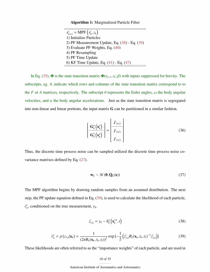
1) Initialize Particles2) PF Measurement Update, Eq. (38) - Eq. (39)3) Evaluate PF Weights, Eq. (40)4) PF Resampling5) PF Time Update6) KF Time Update, Eq. (41) - Eq. (47)

In Eq. (35),� is the state transition matrix�(tk+1, tk; �) with inputs suppressed for brevity. The

subscripts, eg. ✓, indicate which rows and columns of the state transition matrix correspond to to

the F or A matrices, respectively. The subscript ✓ represents the Euler angles, ! the body angular

velocities, and ↵ the body angular accelerations. Just as the state transition matrix is segregated

into non-linear and linear portions, the input matrix G can be partitioned in a similar fashion.

26666666664

Gnk

⇣xn

k

⌘

G`k⇣xn

k

⌘

37777777775=

26666666666666666664

I3⇥3

I3⇥3

I3⇥3

37777777777777777775

(36)

Thus, the discrete time process noise can be sampled utilized the discrete time process noise co-

variance matrixes defined by Eq. (27).

wk ⇠ N (0,Qk(x)) (37)

The MPF algorithm begins by drawing random samples from an assumed distribution. The next

step, the PF update equation defined in Eq. (39), is used to calculate the likelihood of each particle,

cik, conditioned on the true measurement, yk.

zi1,k = yk � hn

k

⇣xi,n

k , t⌘

(38)

cik = p

�z1,k|xk

�=

1(2⇡Rk(xk, tk, tI))2 exp [�1

2

⇣zi

1,kRk(xk, tk, tI)�1zi1,k

⌘] (39)

These likelihoods are often referred to as the “importance weights” of each particle, and are used in

18 of 35


the PF resampling algorithm after normalizing the weights according to Eq. (40). The fourth step,

particle resampling, solves the much discussed shortcoming of the PF, which is sample impover-

ishment. This approach utilizes residual resampling, although other methods such as Metropolis

or stratified resampling have been offered as equally effective alternatives [39].

cik =

cik

NPi=1

cik

(40)

After resampling the particles, they can be propagated to the next time step using a numerical

ordinary differential equation solver. This leads to the final step of this specialized MPF algorithm,

the KF time update. Examining Eq. (34) reveals that the measurement equation is a non-linear

function of the body attitude only. However, the “innovation” term zi2,k defines the couple between

the linear and nonlinear states, as given by Eq. (34).

zi2,k = xi,n

k+1 � Fnn,k

�xn

k�

(41)

It is emphasized that a linearized state-observation mapping relationship is not used here. Addi-

tionally, this is the only means for information from the light curve measurement to be used to

update the linear states. Utilizing this innovation leads to the linear KF propagation and update

equations are given by [21].

x`k+1 = F`kx`k +G`k

⇣Q`nk

⌘T �Gn

kQnk��1 zi

2,k + Lk

⇣zi

2,k � Fnkx`k

⌘(42)

P`k+1 = F`kP`k

⇣F`k

⌘T+G`kQ

`k

⇣G`k

⌘T � LkNkLTk (43)

where it is noted that some parameters have been dropped from the following equations to make

them specific to the light curve inversion problem. The equations necessary for these computations

are given by [21].

Nk = FnkP`k

�Fn

k�T+Gn

kQnk�Gn

k�T (44)

Lk = F`kP`k�Fn

k�T N�1

k (45)

19 of 35


F`k = F`k �G`k⇣Q`nk

⌘T �Gn

kQnk��1 Fn

k (46)

Q`k = Q`k �⇣Q`nk

⌘T �Qn

k��1 Q`nk (47)

These equations complete the MPF algorithm. The MPF affords the estimation of both atti-

tude and angular velocity states of maneuvering space objects, while maintaining computational

tractability. It is also possible that the algorithm could work without knowledge of the initial

orientation of the SO. As alluded to earlier, the initial distribution of the attitude states can be any

arbitrary distribution. It is theoretically possible for the initial distribution to be made uniform over

the attitude states. While not a trivial task, previous work has shown how uniform distributions

can be created for several parameterizations of the SO(3) rotation group including: quaternions,

Rodrigues parameters, axis and angle of rotation, as well as both symmetric and axisymmetric

sequences of Euler angles [40]. Complicating this proposition, is the fact that different angular

velocities lead to the same object brightness. Since the linear, marginalized state is assumed to be

Gaussian-distributed, the MPF could not represent these multiple modes for the body angular ve-

locities. The next section provides some simulated results which highlight these benefits compared

to previous developments.

IV. Simulation Results

The emphasis of this work is to present novel models for improving current attitude estimation

algorithms when applied to agile SOs. If the algorithms presented are to one day be used opera-

tionally, the simulation must match observational data as closely as possible. Accordingly, every

effort is made to create a realistic physics based simulation, as outlined below.

A. Data Flow

The first component of this simulator is the Simplified General Perturbations Propagator (SGP4).

This software calculates the position and velocity of a SO by propagating the information from a

two line element (TLE) file. A MATLAB implementation is available from Vallado et. al. [41] The

next piece of software critical to the simulator is the 1987 implementation of Variations Seculaires

20 of 35


des Orbites Planetaires (VSOP87) [42]. The adaptation of VSOP87 by Bretagnon and Francou [43]

combined with the coordinate transformations provided by Meeus [44] enables the ephemerides of

the Sun and Earth to be calculated with less than 1” error until 6000 A.D. The geometry necessary

to define the reflectance of light can be defined using the the position of the Sun, observer, and

SO. This geometry is used in the final part of the simulator, a bidirectional reflectance distribution

function (BRDF) model. This particular work utilizes the Cook-Torrance BRDF model for specular

contributions [45], and Lambertian reflectance for diffuse contributions to the total radiant flux of

the SO at various attitudes [14].

B. Test Cases

All test cases presented are derived from a two-line element set (TLE) for the NOAA 18 satellite

downloaded from SpaceTrack.org [46]. Each TLE comprises two lines of 80-column ASCII text

identifying the satellite by its catalog ID number and defining its orbital elements at the given

epoch time. The simulation represents observations collected on June 6th, 2014 from 10:19:21 to

10:23:19 UTC from the Fenton Hill Observatory,whose location was modeled as 35.879998� N,

106.293058� W.

NOAA 18 [B]1 28654U 05018A 15024.53745670 .00000182 00000-0 12433-3 0 41472 28654 99.1733 13.7659 0014261 7.4244 99.1613 14.12137281498803

The NOAA 18 spacecraft orbits at a = 7226 km, e = 2.3 ⇥ 10�3, i = 99.2 deg, ⌦ = 17.8 deg,

! = 14.6 deg, and f = 114.8 deg. The problem is simplified such that NOAA 18 is represented by

a simple cube, with the shape model parameters presented in Table 1. In the shape model, A is the

facet area, ⇠ is the affine transformation weighting parameter, a is the diffuse albedo, and m is the

microfacet slope parameter where ⇠, a, and m 2 [0, 1]. Since previous work has addressed shape

model uncertainty, it is assumed the shape model is known perfectly for the purposes of generating

these simulated results [14]. However, the methodology described in this manuscript does not

require that the shape model is known perfectly. Indeed, any practical implementation of these

21 of 35


Table 1: Assumed Shape Model Parameters

Facet A (m2) ⇠ a m+X 2 0.5 0.25 0.3+Y 2 0.5 0.5 0.3+Z 2 0.5 0.75 0.3-X 2 0.5 0.9 0.3-Y 2 0.5 0.4 0.3-Z 2 0.5 0.1 0.3

methods on experimental data will require that the algorithm be capable of handling uncertainties

in these shape model parameters.

To simulate an agile SO, the problem is modeled such that the -Z facet of NOAA 18 is assumed

to remain perpendicular to the zenith originating from Colorado Springs, CO for the duration of the

pass. This results in the acceleration profile depicted in Fig. 2. This simulated mission results in the

Figure 2: True Agile SO Acceleration

light curves presented in Fig. 3. The telescope parameters utilized, shown in Table 2, are those of

the 0.5 m f/8 GT-SORT telescope, and are representative of a typical Raven-class telescope [47].

Ideally, each improvement offered in this work could be introduced as a separate test case.However,

the inclusion of a comparison between the time invariant, limiting magnitude measurement model

and the radiometric measurement model was deemed trivial. Since the benefit afforded by each

improvement is judged by its reduction in the error of estimated states, it seemed illogical to

compare estimates arrived at using a measurement model that produced incorrect uncertainties.

Additionally, it was computationally infeasible to include a comparison between the standard PF

22 of 35


a) TC1 Light Curve b) TC1 Residual vs Time

c) TC2 Light Curve d) TC2 Residual vs Time

e) TC3 Light Curve f) TC3 Residual vs Time

Figure 3: Pre and Post Update Estimate of Light Curve

23 of 35


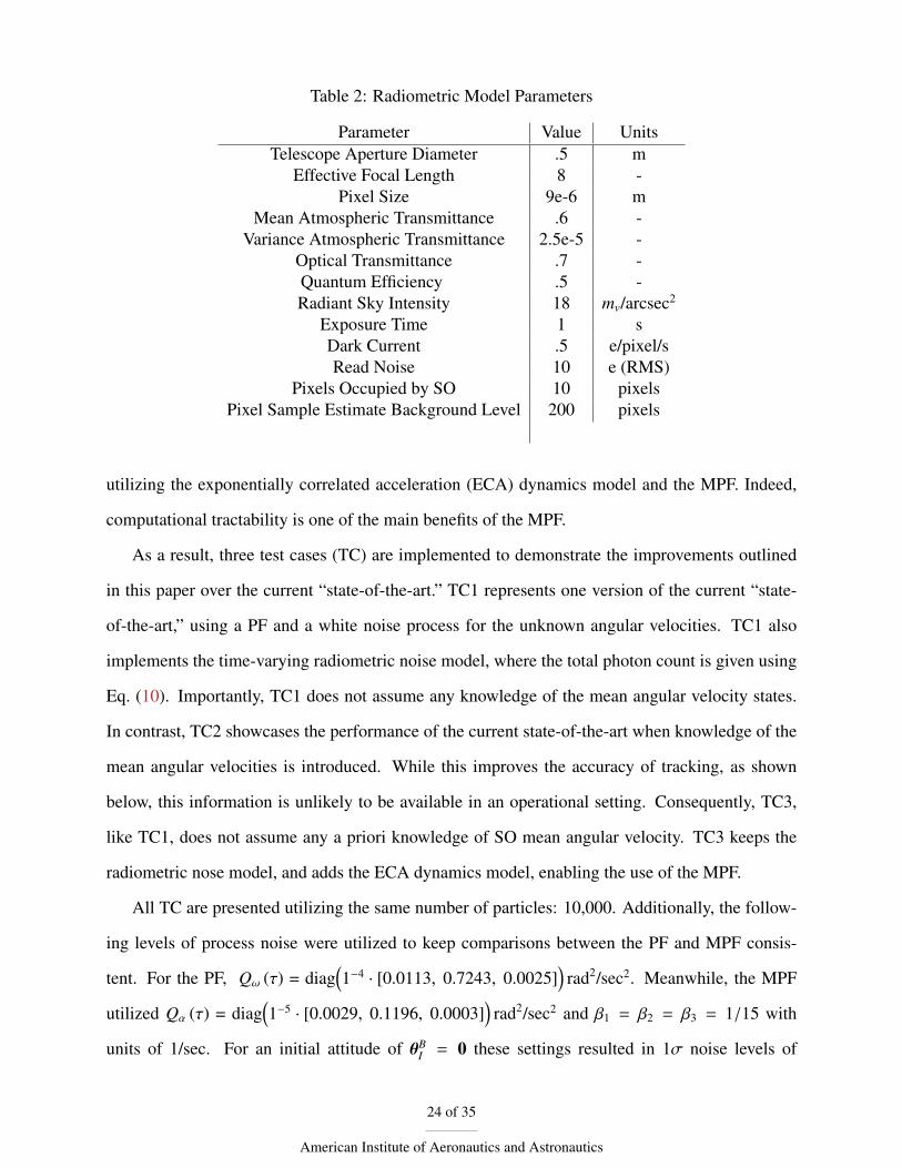
Table 2: Radiometric Model Parameters

Parameter Value UnitsTelescope Aperture Diameter .5 m

Effective Focal Length 8 -Pixel Size 9e-6 m

Mean Atmospheric Transmittance .6 -Variance Atmospheric Transmittance 2.5e-5 -

Optical Transmittance .7 -Quantum Efficiency .5 -Radiant Sky Intensity 18 mv/arcsec2

Exposure Time 1 sDark Current .5 e/pixel/sRead Noise 10 e (RMS)

Pixels Occupied by SO 10 pixelsPixel Sample Estimate Background Level 200 pixels

utilizing the exponentially correlated acceleration (ECA) dynamics model and the MPF. Indeed,

computational tractability is one of the main benefits of the MPF.

As a result, three test cases (TC) are implemented to demonstrate the improvements outlined

in this paper over the current “state-of-the-art.” TC1 represents one version of the current “state-

of-the-art,” using a PF and a white noise process for the unknown angular velocities. TC1 also

implements the time-varying radiometric noise model, where the total photon count is given using

Eq. (10). Importantly, TC1 does not assume any knowledge of the mean angular velocity states.

In contrast, TC2 showcases the performance of the current state-of-the-art when knowledge of the

mean angular velocities is introduced. While this improves the accuracy of tracking, as shown

below, this information is unlikely to be available in an operational setting. Consequently, TC3,

like TC1, does not assume any a priori knowledge of SO mean angular velocity. TC3 keeps the

radiometric nose model, and adds the ECA dynamics model, enabling the use of the MPF.

All TC are presented utilizing the same number of particles: 10,000. Additionally, the follow-

ing levels of process noise were utilized to keep comparisons between the PF and MPF consis-

tent. For the PF, Q! (⌧) = diag⇣1�4 · [0.0113, 0.7243, 0.0025]

⌘rad2/sec2. Meanwhile, the MPF

utilized Q↵ (⌧) = diag⇣1�5 · [0.0029, 0.1196, 0.0003]

⌘rad2/sec2 and �1 = �2 = �3 = 1/15 with

units of 1/sec. For an initial attitude of ✓BI = 0 these settings resulted in 1� noise levels of

24 of 35


�!0 = [0.061, .488, .029]T deg/sec.

Table 3: Test Case Descriptions

Test Case NL/L States Measurement Model Dynamics Model !µ Filter#1 3/0 Radiometric White-Noise 0 PF#2 3/0 Radiometric White-Noise Truth PF#3 3/6 Radiometric ECA 0 MPF

Fig. 4 through Fig. 7 illustrate the particle clouds of the three test cases at four instances during

the simulation time. TC1 is always presented on the top row, while the middle and bottom rows

are TC2 and TC3 respectively. The particles themselves are shaded such that the particles with the

highest likelihoods, i.e. weights, are shown in black while particles that represent less likely states

are represented with lighter shades of gray. In all subfigures, the true simulated state is shown with

a red star.

Fig. 4 illustrates the initialized particles for all test cases. In all test cases, the particles are

uniformly distributed in Euler angle space in a window around the true state. This is purely a

constraint of the computational resources available to the authors. Given a high performance com-

puter, both the PF and MPF filters are capable of uniformly sampling the entire state space. Fig. 5

shows both filters 75 seconds into the simulation. One can see that the particles of the MPF (TC3)

are distributed in smaller volume of state space than either PF test case. Additionally, the large

swaths of gray particles in TC1 and TC2 highlight that the MPF is much more computationally

efficient, with each resampled particle having a higher liklihood according to Eq. (39).

Fig. 6 shows both filters 155 seconds into the simulation, and is an excellent illustration of the

highly non-Gaussian distributions typical of the SO attitude estimation problem. It is also evident

by examining TC1 that without knowledge of the SO’s mean angular velocity, the state of the art

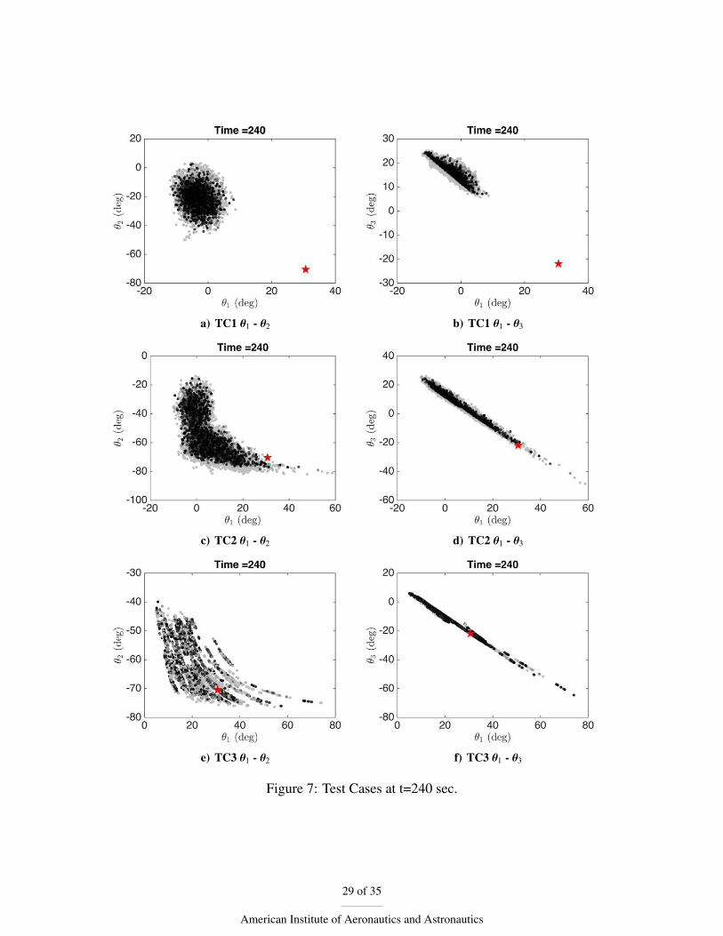
PF begins to diverge, with the true SO state no longer bounded by the particle cloud. Fig. 7 shows

all test cases at the final time step in the simulation, at 240 seconds. Only in TC2 and TC3 is the

SO successfully tracked, with the true state contained within the particle cloud. The left hand side

of Fig. 8 shows the true SO attitude, denoted by the solid black line, compared to the first moment

of the particle cloud, shown by black circles, along with the 5 and 95 percentile bounds of the

particle cloud illustrated by the shaded gray area. The right hand side of Fig. 8 shows the residuals

25 of 35


a) TC1 ✓1 - ✓2 b) TC1 ✓1 - ✓3

c) TC2 ✓1 - ✓2 d) TC2 ✓1 - ✓3

e) TC3 ✓1 - ✓2 f) TC3 ✓1 - ✓3

Figure 4: Test Cases at t=0 sec.

26 of 35


a) TC1 ✓1 - ✓2 b) TC1 ✓1 - ✓3

c) TC2 ✓1 - ✓2 d) TC2 ✓1 - ✓3

e) TC3 ✓1 - ✓2 f) TC3 ✓1 - ✓3


27 of 35


a) TC1 ✓1 - ✓2 b) TC1 ✓1 - ✓3

c) TC2 ✓1 - ✓2 d) TC2 ✓1 - ✓3

e) TC3 ✓1 - ✓2 f) TC3 ✓1 - ✓3


28 of 35


a) TC1 ✓1 - ✓2 b) TC1 ✓1 - ✓3

c) TC2 ✓1 - ✓2 d) TC2 ✓1 - ✓3

e) TC3 ✓1 - ✓2 f) TC3 ✓1 - ✓3


29 of 35


of the attitude state, denoted by black ‘X’, along with the 5 and 95 percentile residual bounds.

It is important to grasp the physical reason why the percentile bounds grow as observations of

the SO are collected. This is directly due to the interaction between the measurement noise and

process noise. The observing environment described in Table 2 is shot-noise limited and in this

anecdotal example the SO being observed becomes brighter with time, as shown in the left hand

subfigures of Fig. 3. Consequently, the shot noise increases the measurement noise during the

simulation, as defined in Eq. (9). This increase in measurement noise causes more particles around

the truth to represent brightness values consistent with the measurement statistics. As a result, the

particles which have been randomly subjected to higher levels of process noise are not eliminated,

and the cloud of particles grows as the simulation progresses.

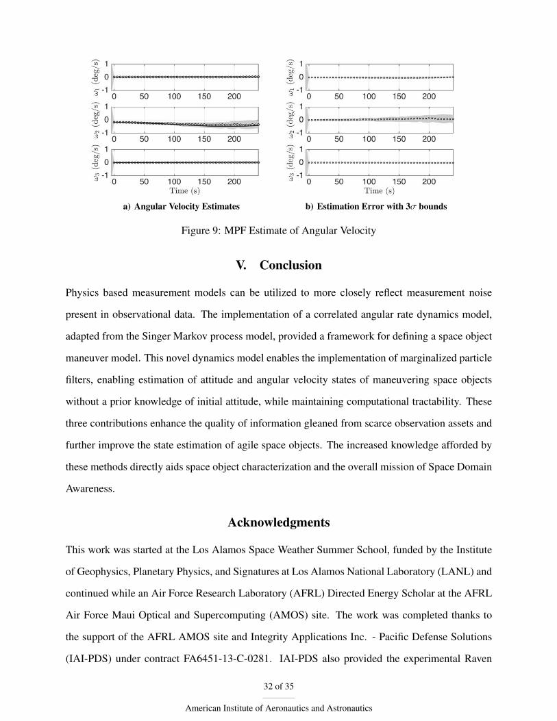
Only through the novel contributions of this work, illustrated in TC3, are the angular velocity

states able to be simultaneously estimated. Fig. 9b gives the body angular velocities provided by

the KF update portion of the MPF. The estimation error is given by the solid black line, while the

5 and 95 percentile bounds are given by the shaded gray area. The ability of the MPF to provide

angular velocity estimates, via the adoption of the Singer dynamics model, is a novel improvement

to the SO attitude estimation problem.

The first benefit of this ability is that knowledge of SO body angular velocity can be used to

better estimate the attitude states via the KF update step of the MPF. This benefit is evident in Fig.

4 through Fig. 7, where the volume of state space occupied by the particle cloud is less for the

MPF than the PF. The second benefit afforded by knowledge of SO angular velocities manifests

itself in SO operational mode classification. While determining the current attitude of a SO is a

critical aspect of characterization, it is not an immediately actionable piece of information. Indeed,

SSA stakeholders desire information on the operational mode of a SO, e.g. if the SO is currently

Sun-pointing, nadir-pointing, or tracking another SO. Information on SO angular velocity could be

an important discriminator in operational mode classification if multiple operational classifications

are represented by similar SO attitude states alone.

30 of 35


a) TC1 Attitude Estimates b) TC1 Attitude Residuals

c) TC2 Attitude Estimates d) TC2 Attitude Residuals

e) TC3Attitude Estimates f) TC3 Attitude Residuals

Figure 8: Comparison of Attitude Estimates

31 of 35


a) Angular Velocity Estimates b) Estimation Error with 3� bounds

Figure 9: MPF Estimate of Angular Velocity

V. Conclusion

Physics based measurement models can be utilized to more closely reflect measurement noise

present in observational data. The implementation of a correlated angular rate dynamics model,

adapted from the Singer Markov process model, provided a framework for defining a space object

maneuver model. This novel dynamics model enables the implementation of marginalized particle

filters, enabling estimation of attitude and angular velocity states of maneuvering space objects

without a prior knowledge of initial attitude, while maintaining computational tractability. These

three contributions enhance the quality of information gleaned from scarce observation assets and

further improve the state estimation of agile space objects. The increased knowledge afforded by

these methods directly aids space object characterization and the overall mission of Space Domain

Awareness.

Acknowledgments

This work was started at the Los Alamos Space Weather Summer School, funded by the Institute

of Geophysics, Planetary Physics, and Signatures at Los Alamos National Laboratory (LANL) and

continued while an Air Force Research Laboratory (AFRL) Directed Energy Scholar at the AFRL

Air Force Maui Optical and Supercomputing (AMOS) site. The work was completed thanks to

the support of the AFRL AMOS site and Integrity Applications Inc. - Pacific Defense Solutions

(IAI-PDS) under contract FA6451-13-C-0281. IAI-PDS also provided the experimental Raven

32 of 35


data included in this work. A special thanks is due to Dr. David Palmer of LANL, Kris Hamada

of IAI-PDS, and Dr. Chris Sabol and Dr. Kim Luu of AFRL for their insightful and thought

provoking feedback.

References[1] D. H. Rumsfeld, “Commission to Assess United States National Security Space Management and

Organization,” tech. rep., Committee on Armed Services of the U.S. House of Representatives, January2001.

[2] Joint Chiefs of Staff, “Space Operations,” Tech. Rep. JP 3-14, United States Department of Defense,May 2013.

[3] G. Stokes, C. Von Braun, R. Sridharan, D. Harrison, and J. Sharma, “The Space-Based Visible Pro-gram,” Lincoln Laboratory Journal, Vol. 11, No. 2, 1998, pp. 205–238, 10.2514/6.2000-5334.

[4] D. Hall, B. Calef, K. Knox, M. Bolden, and P. Kervin, “Separating attitude and shape effects for non-resolved objects,” Advanced Maui Optical and Space Surveillance Technologies Conference, 2007,pp. 464–475.

[5] J. L. Walker, “Range-Doppler imaging of rotating objects,” Aerospace and Electronic Systems, IEEETransactions on, No. 1, 1980, pp. 23–52, 10.1109/taes.1980.308875.

[6] D. Hall, J. Africano, P. Kervin, and B. Birge, “Non-Imaging Attitude and Shape Determination,” Ad-vanced Maui Optical and Space Surveillance Technologies Conference, September 2005.

[7] J. Dunlap, “Lightcurves and the axis of rotation of 433 Eros,” Icarus, Vol. 28, No. 1, 1976, pp. 69–78,10.1016/0019-1035(76)90087-7.

[8] P. Magnusson, “Distribution of spin axes and senses of rotation for 20 large asteroids,” Icarus, Vol. 68,No. 1, 1986, pp. 1 – 39, DOI: 10.1016/0019-1035(86)90072-2.

[9] M. Kaasalainen, L. Lamberg, K. Lumme, and E. Bowell, “Interpretation of lightcurves of atmosphere-less bodies. I - General theory and new inversion schemes,” Astronomy and Astrophysics, Vol. 259,June 1992, pp. 318–332.

[10] M. Kaasalainen, L. Lamberg, and K. Lumme, “Interpretation of lightcurves of atmosphereless bodies.II - Practical aspects of inversion,” Astronomy and Astrophysics, Vol. 259, June 1992, pp. 333–340.

[11] J. Torppa, M. Kaasalainen, T. Michalowski, T. Kwiatkowski, A. Kryszczynska, P. Denchey, andR. Kowalski, “Shapes and rotational properties of thirty asteroids from photometric data,” Icarus,Vol. 164, No. 1, 2003, pp. 364–383, doi:10.1016/S0019-1035(03)00146-5.

[12] C. J. Wetterer and M. K. Jah, “Attitude Determination from Light Curves,” AIAA Journal of Guidance,Control, and Dynamics, Vol. 32, September-October 2009, pp. 1648–1651, 10.2514/1.44254.

[13] R. D. Coder and M. J. Holzinger, “Multi-Objective Design of Optical Systems for Space SituationalAwareness,” Acta Astronautica, 2015.

[14] M. J. Holzinger, K. T. Alfriend, C. J. Wetterer, K. K. Luu, C. Sabol, and K. Hamada, “Photometricattitude estimation for agile space objects with shape uncertainty,” Journal of Guidance, Control, andDynamics, Vol. 37, No. 3, 2014, pp. 921–932, 10.2514/1.58002.

33 of 35


[15] R. Singer, “Estimating Optimal Tracking Filter Performance for Manned Maneuvering Targets,”IEEE Transactions on Aerospace and Electronic Systems, Vol. AES-6, July 1970, pp. 473 –483,10.1109/TAES.1970.310128.

[16] J. Fitts, “Aided tracking as applied to high accuracy pointing systems,” IEEE Transactions onAerospace and Electronic Systems, Vol. 3, No. AES-9, 1973, pp. 350–368.

[17] J. B. Pearson and E. B. Stear, “Kalman filter applications in airborne radar tracking,” IEEE Transac-tions on Aerospace and Electronic systems, No. 3, 1974, pp. 319–329.

[18] W. Blair, G. Watson, and T. Rice, “Tracking maneuvering targets with an interacting multiple modelfilter containing exponentially-correlated acceleration models,” System Theory, 1991. Proceedings.,Twenty-Third Southeastern Symposium on, IEEE, 1991, pp. 224–228.

[19] X. R. Li and V. P. Jilkov, “Survey of maneuvering target tracking. Part I. Dynamic models,” Aerospaceand Electronic Systems, IEEE Transactions on, Vol. 39, No. 4, 2003, pp. 1333–1364.

[20] A. Doucet, N. J. Gordon, and V. Krishnamurthy, “Particle filters for state estimation of jump Markovlinear systems,” Signal Processing, IEEE Transactions on, Vol. 49, No. 3, 2001, pp. 613–624.

[21] T. Schon, F. Gustafsson, and P.-J. Nordlund, “Marginalized particle filters for mixed linear/nonlinearstate-space models,” Signal Processing, IEEE Transactions on, Vol. 53, No. 7, 2005, pp. 2279–2289,10.1109/tsp.2005.849151.

[22] E. Budding and O. Demircan, Introduction to Astronomical Photometry. Cambridge Ob-serving Handbooks for Research Astronomers, Cambridge University Press, 2nd ed., 2007,10.1017/CBO9780511536175.

[23] J. R. Shell, “Optimizing Orbital Debris Monitoring with Optical Telescopes,” Advanced Maui Op-tical and Space Surveillance Technologies Conference, Space Innovation and Development Center,September 2010.

[24] J. R. Schott, Remote Sensing: The Image Chain Approach. Oxford University Press, 1997.

[25] W. Merline and S. B. Howell, “A Realistic Model for Point-sources Imaged on Array Detectors:The Model and Initial Results,” Experimental Astronomy, Vol. 6, No. 1-2, 1995, pp. 163–210,10.1007/BF00421131.

[26] T. Schildknecht, “Optical Astrometry of Fast Moving Objects Using CCD Detectors,” Geodatisch-geophysikalische Arbeiten in der Schweiz, Vol. 49, 1994.

[27] W. W. Hines, D. C. Montgomery, C. M. Borror, and D. M. Goldsman, Probability and Statistics inEngineering. Wiley, 2008.

[28] R. Linares, M. K. Jah, J. L. Crassidis, and C. K. Nebelecky, “Space Object Shape Characterization andTracking Using Light Curve and Angles Data,” Journal of Guidance, Control, and Dynamics, Vol. 37,No. 1, 2013, pp. 13–25, 10.2514/1.62986.

[29] D. Dravins, L. Lindegren, E. Mezey, and A. T. Young, “Atmospheric intensity scintillation of stars.I. Statistical distributions and temporal properties,” Publications of the Astronomical Society of thePacific, 1997, pp. 173–207.

[30] C. Rose and M. D. Smith, “MathStatica: mathematical statistics with mathematica,” Compstat,Springer, 2002, pp. 437–442.

34 of 35


[31] M. C. Roggemann, B. M. Welsh, and B. R. Hunt, Imaging through turbulence. CRC press, 1996.

[32] E. D. Feigelson and G. J. Babu, Modern Statistical Methods for Astronomy: with R Applications.Cambridge University Press, 2012, 10.1017/CBO9781139015653.

[33] D. Karlis and E. Xekalaki, “Mixed poisson distributions,” International Statistical Review, Vol. 73,No. 1, 2005, pp. 35–58.

[34] R. Berg, “Estimation and prediction for maneuvering target trajectories,” IEEE Transactions on Auto-matic Control, Vol. 28, No. 3, 1983, pp. 294–304.

[35] K. Kumar and H. Zhou, “A ’current’ statistical model and adaptive algorithm for estimating maneu-vering targets,” Journal of guidance, control, and dynamics, Vol. 7, No. 5, 1984, pp. 596–602.

[36] S. Blackman and R. Popoli, “Design and analysis of modern tracking systems,” Norwood, MA: ArtechHouse, 1999., 1999.

[37] N. Nabaa and R. H. Bishop, “Validation and comparison of coordinated turn aircraft maneuver mod-els,” IEEE Transactions on aerospace and electronic systems, Vol. 36, No. 1, 2000, pp. 250–259.

[38] A. H. Jazwinski, Stochastic Processes and Filtering Theory. Courier Dover Publications, 2007.

[39] R. Douc and O. Cappe, “Comparison of resampling schemes for particle filtering,” Image and SignalProcessing and Analysis, 2005. ISPA 2005. Proceedings of the 4th International Symposium on, IEEE,2005, pp. 64–69.

[40] M. D. Shuster, “Uniform attitude probability distributions,” Journal of Astronautical Sciences, Vol. 51,No. 4, 2003, pp. 451–475.

[41] D. A. Vallado, P. Crawford, R. Hujsak, and T. Kelso, “Revisiting spacetrack report# 3,” AIAA,Vol. 6753, 2006, p. 2006.

[42] P. Bretagnon and G. Francou, “Planetary theories in rectangular and spherical variables-VSOP 87solutions,” Astronomy and Astrophysics, Vol. 202, 1988, pp. 309–315.

[43] P. Bretagnon and G. Francou, “Planetary theories in rectangular and spherical variables-VSOP 87solutions,” Astronomy and Astrophysics, Vol. 202, 1988, pp. 309–315.

[44] J. H. Meeus, Astronomical algorithms. Willmann-Bell, Incorporated, 1991.

[45] R. L. Cook and K. E. Torrance, “A Reflectance Model for Computer Graphics,” Computer Graphics,Vol. 15, August 1981, pp. 307–316.

[46] “Space-Track.org,” June 2015, www.space-track.org.

[47] C. Sabol, K. K. Luu, P. Kervin, D. Nishimoto, K. Hamada, and P. Sydney, “Recent Developments ofthe Raven Small Telescope Program,” AAS/AIAA Space Flight Mechanics Meeting, Vol. AAS 02-131,2002, p. 397.

35 of 35


3dof estimation of agile space objects using marginalized ...rlinares/papers/2017_02.pdf · 3dof...

Documents