Junping CaiM.Sc. E. E, PhD

junping@mci.sdu.dk

Centre for Product Development (CPD) Mads Clausen Institute (MCI)

University of Southern Denmark(SDU) 2011

3D Motion Trackingby Inertial and Magnetic sensors

with or without GPS

Outline Short introduction of Junping Cai Coordinate Systems Inertial Motion Tracking Working Principle On-site Calibration Extended Kalman Filter without GPS Extended Kalman Filter with GPS Experiment results Application examples Discussions

Short introduction of Junping

Come from China

1988-1992, B.Sc., Automatic Control, Department of Automatic Control, Nanjing University of Aeronautics and Astronautics, China

1992-1996, Production Engineer, Canon (Tianjin) Ltd., China 1996-2002, Purchasing Engineer, Danfoss (Tianjin) Ltd., China 2002-2004, M.Sc., Mechatronics Engineering, Mads Clausen Institute

(MCI),University of Southern Denmark (SDU), Denmark 2004-2007, PhD Student, Automation & Control, Department of Electronic

Systems,Aalborg University, Denmark, Supervisors: Professor Jakob Stoustrup 2008 – 2009, Lead Development Engineer, Automatic Controls Laboratories,

Danfoss A/S, Denmark 2009—now, R & D Engineer, Centre for Product Development

(CPD),MCI,SDU

Coordinate systems

Relations between ECEF-frame (e), local geodetic-frame (t) and inertial-frame (i) .

Earth-Centered Earth-Fixed Frame (ECEF, e-frame)

Inertial Frame (i-frame)

Local Geodetic Frame (t-frame) Local Tangent Plane (LTP)(N-frame, global) North- East- Down (NED) East- North- Up (ENU)

Body Frame (b-frame,local)ForwardRightDown

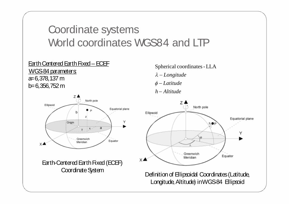
Coordinate systemsWorld coordinates WGS84 and LTP

Earth-Centered Earth Fixed (ECEF) Coordinate System

Earth Centered Earth Fixed – ECEFWGS‐84 parameters: a=6,378,137 mb=6,356,752 m

Definition of Ellipsoidal Coordinates (Latitude, Longitude, Altitude) in WGS-84 Ellipsoid

AltitudehLatitudeLongitude

LLA -scoordinate Spherical

Inertial motion tracking working principle

Integral

Projection to global IntegralIntegralCorrect

gravity

3-axis GyroAngular Rate

3 -axis AccelerometerAcceleration

Orientation

Velocity Position

Initial Velocity

Initial Position

zyx aaaterAccelerome

zyx ωωωGyroscope North

East

Up

Global system

nOrientatio

Position

Velocity

ZYX

ZYX

PPP

VVVEuler AnglesQuaternion

Rotation vector

Coordinate Transformation

local system

‘The Devil is in the details’

Linear Acceleration

Quaternion attitude representation-for example

00

00

)(

)())(()(),()(

)(21

021)(

update Quaternion

22)12()(Local) to(Globalmatrix tion Transforma

Quaternion

24411

)()()(

43324

4321

zyx

zxy

yxz

xyz

kL

Gt

kL

GkkkL

G

tLG

tLG

tLG

TLG

tqtqtttq

qqtq

qqqqIqqC

qkqjqiqq

C(1,1))C(1,2),(atan Yaw

C(1,3))asin(- Pitch

C(3,3))C(2,3),(atan Rollgravity-g

position

velocity

aon acceleratilinear

)(

LG

LG2

LG

LG

LG2

00

00

linear

1

tf

t

tf

t linear

ENU

z

y

xL

G

U

N

E

VdtPP

dtaVV

ga

aaa

qCaaa

Transformation

Calibration Why:

Low cost Suffer from the time drift Sensitivity to the environmental parameters

Purpose is to in-field determine : The Bias The Scale factor (Gain) The Orientation (misalignment)

Requirement Time Complexity Instruments ...

3-axis Acc

3-axis Gyro

Support base

Sensors case

3-axis Mag

Orientation -Misalignment Misalignment: Nominal sensitivity axis vs. Actual sensitivity axis

r

r

r

r

rr

sinsincossin

cos

1rUnit vecto

,r ,raxisy sensitivit Actual

222

rrrrrr

rrr

r

Accelerometer calibration example

5342,15288,14985,1

Ba

9996,0015,00250,00098,09999,00049,00251,00050,09997,0

Ra

0 2 4 6 8 10 12 14

x 104

-2

-1.5

-1

-0.5

0

0.5

1

1.5

2

axa

yaza

tot

330] 300 [270max] [min typ

ionspecificatsheet Data1,29300

08,2980006,291

Ka

0 2 4 6 8 10 12 14

x 104

0

200

400

600

800

1000

1200

a

xayazax,fay,fa

z,f

Raw and filtered data

Calibrated data

On-field fast calibration-Magnetometers

Method I: Using Earth Magnetic Field as Known Input, Publication ION 2010

Method II: 3D Ellipsoid Curve Fitting Method III: 2D Mapping (boat & car)

Alsion 2 for example (WMM 2010)Latitude = 54.91; % Degree NLongitude = 9.78; % Degree EAltitude = 0.00; % KmDate = 2011.2;F = 49826.4e-5; % nT 2 GaussH = 17513.6e-5; % nT 2 GaussX = 17506.3e-5; % nT 2 GaussY = 505.1e-5; % nT 2 GaussZ = 46647.0e-5; % nT 2 GaussDecl = 1 + 39/60; % (Degree East)Incl = 69+ 25/60; % (Down) (Dip)

Alsion 2 for example (WMM 2010)Latitude = 54.91; % Degree NLongitude = 9.78; % Degree EAltitude = 0.00; % KmDate = 2011.2;F = 49826.4e-5; % nT 2 GaussH = 17513.6e-5; % nT 2 GaussX = 17506.3e-5; % nT 2 GaussY = 505.1e-5; % nT 2 GaussZ = 46647.0e-5; % nT 2 GaussDecl = 1 + 39/60; % (Degree East)Incl = 69+ 25/60; % (Down) (Dip)

Magnetic declination is the angle between magnetic north (the direction the north end of a compass needle points) and true north(north pole). The declination is positive when the magnetic north is east of true north.

On-field fast calibration-Magnetometers

Requirement: Many different orientations

as possible. e.g. keep the object still for a few seconds in at least 12 significantly different orientations, preferably more

At least 3 meters from large ferromagnetic objects such as radiators and iron desks

mapping 3D :III Method

555560

565525

530

440

445

450

455

Magnetic field raw data

-0.4 -0.2 0 0.2 0.4 -0.4-0.2

00.2

0.4-0.4

-0.2

0

0.2

0.4

Magnetic field calibrated data

222

z

zz

y

yy

x

xx

kbh

kbh

kbhF

On-field fast calibration-Magnetometers 2D mapping example

0 10 20 30 40 50 60-0.5

0

0.5

1Magnetic Field Raw Data

Mag

netic

[Gau

ss]

0 10 20 30 40 50 60-0.5

0

0.5

1

Time [s]

Mag

netic

[Gau

ss]

Magnetic Field Calibrated Data

BR

BP

BYBtot

Btot,t

-0.6 -0.4 -0.2 0 0.2 0.4 0.6

-0.2

-0.1

0

0.1

0.2Horizontal Projection

[Gau

ss]

[Gauss]

beforeaftertrue

0 10 20 30 40 50 600.4

0.5

0.6

0.7

0.8Vertical Projection

[Gau

ss]

time [s]

On-field calibration No special instrument is needed No special training is needed No strict sensor alignment (when mounting) is need First we do the factory calibration Then user do the on-site (on-use) calibration

1. User need to stand still (if mounted) or hold the sensor set still for a few seconds

2. User turns around 360 degree (if mounted) or rotate the sensor set in space

Automatic and fast!

Extended Kalman Filter without GPSEvent detection and Constraints

Error Estimates

IMU Navigation Processor

Kalman FilterKalman Filter

Position Velocity Attitude

Error estimates

Closed loop

MagnetometerN-Navigation coordinate (NED)b- sensor body coordinate

Constraints

Event detector

Event detector

Extended Kalman Filter with GPS Loosely coupled integration strategy

Error Estimates

IMU Navigation Processor

Kalman FilterKalman Filter

Position Velocity Attitude

Error estimates

Closed loop

GPS

MagnetometerN-Navigation coordinate (NED)b- sensor body coordinate

Constraints

Experiments (indoor)

Walking a straight line

-1 -0.5 0 0.5 10

0.2

0.4

0.6

0.8

1

1.2

1.4

1.6

1.8

2

Position

Right[m]

Forw

ard

[m]

0 5 10 15 20 25 30-20

0

20Acceleration measurement in RPY

time [sec]Acc

eler

atio

n [m

/s2 ]

AR

APAY

Atot

0 5 10 15 20 25 30-10

0

10Linear Acceleration in NED

time [sec]Acc

eler

atio

n [m

/s2 ]

AN

AE

AD

0 5 10 15 20 25 30-5

0

5Velocity

time [sec]

Vel

ocity

[m/s

]

VN

VE

VD

Indoor pedestrian tracking

Experiment (outdoor)Landyacht with GPS

Alsion parking lot

Experiment Results

0 50 100 150 200-5

0

5Roll angle [degree]

0 50 100 150 200-20

-15

-10Pitch angle [degree]

0 50 100 150 200

-1000

100

Yaw angle [degree]

Experiment Results

0 50 100 150 200-3

-2

-1

0

1

2

3

time [s]

Vel

ocity

[m/s

]

Velocity in NED

VN

VEVD

0 50 100 150 200-1

-0.5

0

0.5

1

1.5

2

time [s]

Acc

eler

atio

n [m

/s2 ]

Linear Acceleration

Experiment Results

0 20 40 60 80 100 120 140 160 180 200-150

-100

-50

0

50

100Position in NED

time [sec]

Pos

ition

[m]

PN

PEPD

INS: Fs=100 Hz GPS: Fs=1 HzBlack line -INS. Colored line-GPS 24 25 26 27 28 29

-16

-15

-14

-13

-12

-11

-10

-9

time [sec]

Pos

ition

[m]

Position in NED

Zoomed in

Experiment results

-20 0 20 40 60 80 100 120-140

-120

-100

-80

-60

-40

-20

0

20

Nor

th [m

]

East [m]

Position and Velocity direction

PEN

VcalVGPS

What during GPS signal blockage (outage) periods

The consequence of GPS outage Bridging algorithm Optimal Backward Smoothing (OBS) DBM algorithm1

Positioning errors in INS/GPS navigation applications

Positioning (North) errors between INS/GPS with GPS outage at 40s-50s and 130s-150s

0 50 100 150 200-10

0

10

20

30

40

50

60

70

80

time [sec]

Pos

ition

[m]

Position NED error between INS and GPS

Optimal backward smoothing (OBS)algorithm

Three classes of OBS algorithms fixed-interval smoother

[0 N]

fixed-point (single-point ) smoother

fixed-lag smoother

Application dependent: Post-mission: the fixed-interval Near real-time: the fixed-lag Initial condition: the fixed- point

Categories of OBS algorithms adapted from Nassar 2003

Nmkk

] 1[ Nkjkj

beginingb ende

)(21

outage theduringerror position expected The)(

)(2outage GPS duringparameter error on Accelerati

,,,,,

,,,,,

2

2,,

bGPSibINSibi

eGPSieINSiei

beii

be

bieii

rrrrrr

ttaDBM

ttrr

a

0 50 100 150 200-140

-120

-100

-80

-60

-40

-20

0

20

40

time [sec]

Pos

ition

[m]

Position in NED

DBM algorithm

Scenario shows the effect of backward smoothing (Simulated data with manipulated GPS signal)

red solid line-when GPS outage. red dotted line- GPS true position, black line -smoothed data

Uniqueness of the product

• Compact design: 27.9 x 19.5 x 4.8 mm3, 2 gram + battery • Battery (rechargeable) driven, battery time: 4 - 200 hour• SIM card data storage + USB data transfer/battery charging• 25 sensors hardware and software• 3D gyro, 3D accelerometer, 3D magnetometer, temperature and internal

voltages.• Heading, roll and pitch, velocity, position, angular velocity, acceleration.• Time stamping• RF data transmission /receiving • Advanced batch and data processing and filtering

Applications

Medical /Biomechanical study

Rehabilitation

Sport training

….

Application example: medicalRemote Monitoring of Patients With Parkinson’s Disease (PD)

3D Acceleration

3D Angular velocity

3D (Magnetic)

Normal

Hyper-kinesias

Dystonia

Slow

Freezing

Kalman Filter+Translation+ Pattern recognition

X

Y

Movement pattern of PD patients• normal movements • slowing of movements • hyperkinesias (exaggerated abnormal movements) • dystonia (abnormal tone in a limb) • freezing (no movements)

Time (sec)

Freq

uenc

y (H

z)

Spectrogram of test signal

0 50 100 1500246

0 50 100 1500

2

Time (sec)

Am

plitu

de (g

)

Original test signal

0 50 100 150

204060

Time (sec)

Pow

er ra

tio (%

)

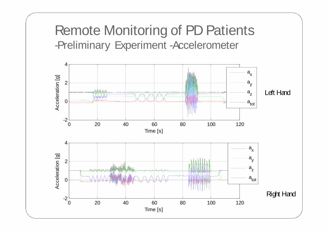
Remote Monitoring of PD Patients-Preliminary Experiment -Accelerometer

0 20 40 60 80 100 120-2

0

2

4

Time [s]

Acc

eler

atio

n [g

]

ax

ay

az

atot

0 20 40 60 80 100 120-2

0

2

4

Time [s]

Acc

eler

atio

n [g

]

ax

ay

az

atot

Left Hand

Right Hand

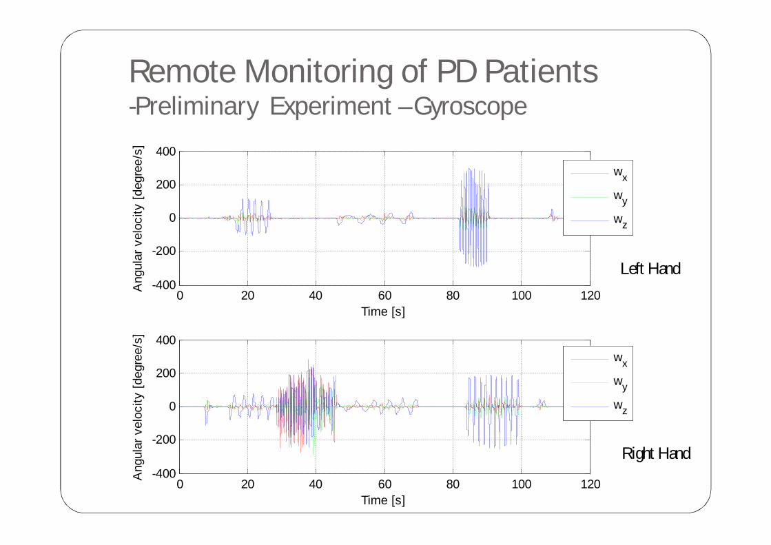
Remote Monitoring of PD Patients-Preliminary Experiment –Gyroscope

0 20 40 60 80 100 120-400

-200

0

200

400

Time [s]

Ang

ular

vel

ocity

[deg

ree/

s]

wx

wy

wz

0 20 40 60 80 100 120-400

-200

0

200

400

Time [s]

Ang

ular

vel

ocity

[deg

ree/

s]

wx

wy

wz

Right Hand

Left Hand

Application example: Medical/ biomechanical study

Life/KU (Copenhagen University)Detection and quantification of lameness in horses Symmetric /Asymmetric

Structure and Motion Laboratory,The Royal Veterinary College, UK Royal National Orthopaedic Hospital, UKStudy of locomotion

Displacement data for x (craniocaudal), y (lateral) and z (dorsoventral) movement m, and orientation data , for optical motion capture (blue) and inertialsensor (red) for a series of strides at canter (9m/s)Structure and Motion laboratory, UK

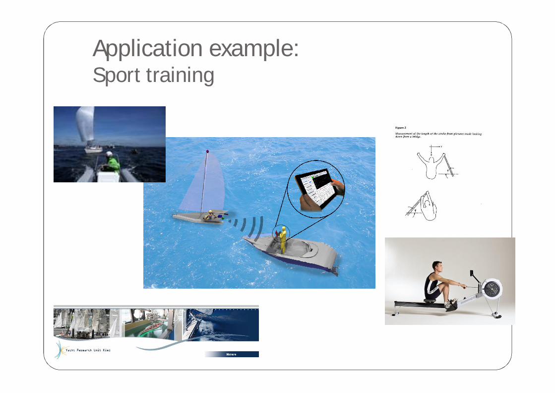
Application example: Sport training

Application example: Rehabilitation/welfare

Application example: Rehabilitation/welfare

Applications: Sports/rehabilitation

Physical segment model and the definition of its orthogonal frame

Depiction of the 15 segments comprising stick figure for human body

Applications: sports/rehabilitation

Relation between the measurements in segment (i) and segment (i+1)

Transpose-Tfield magnetic-H

gravity-ganglejoint theis

1iisegment fromector rotation v theis

),(

),(

1

1111

1111

ii

Tiz

iy

ix

ii

Tiz

iy

ix

Tiz

iy

ix

ii

Tiz

iy

ix

Kwhere

HHHKRotHHH

gggKRotggg

The whole body movement can be calculated by a series of Translation & Rotation.

There is no need for strict sensor alignment.

Discussions

Do we need so many sensors?

What are the cost of sensors

What is the accuracy of the measurement?

Discussion 1–Do we need so many sensors?

Sensor dependent

roll pitch yaw

Gyroscope Optical (Sagnac Effect )

Ring Laser Gyroscope (RLG) Fiber Optic Gyroscope (FOG)

Mechanical MEMS (Micro-Electro-Mechanical Systems) Gyroscope

Accelerometer

Gyroscope

Magnetometer

Discussion 1 –cont.Do we need so many sensors

When the time frequency matter – accelerometer only is enough

• Application dependent

Time (sec)

Freq

uenc

y (H

z)

Spectrogram of test signal

0 50 100 1500246

0 50 100 1500

2

Time (sec)

Am

plitu

de (g

)

Original test signal

0 50 100 150

204060

Time (sec)

Pow

er ra

tio (%

)

Discussion 1 –cont.Do we need so many sensors

When the angle and linear acceleration matter: gyroscope+ accelerometer + magnetometer

• Application dependent

Discussion 2 What are the cost of sensors

Accelerometers

Magnetometers

Discussion 3What is the accuracy of the measurement? Periodic (cyclic) movement Walking (on one plane / on multi-plane ) Running Hurdles Pole jumping (vaulting)

No cyclic / Random movement (outdoors with GPS )…

No cyclic / Random movement (indoors, e g upper limb movement)- biomechanical model is need

Summary

We can fuse gyroscopes, accelerometers, magnetometers (and GPS data ) to deliver accurate and reliable motion information, and output:• Quaternion/

Transformation matrix /Rotation vector

• Heading, pitch, and roll• Linear acceleration• Velocity • Position

Hardware Software

Mathematic On-site calibration

Data fusion

Mathematic On-site calibration

Data fusion

Biomechanical models

Application knowledge

Some inspirations:

Click and play the videohttp://www.xsens.com/en/mvn-biomech