3d experimental and numerical analysis of wind flow around domed-roof buildings with open and closed...

Research Article

Architecture and H

uman

Behavior

E-mail: [email protected]

3D experimental and numerical analysis of wind flow around domed-roof buildings with open and closed apertures

Ali Rahmatmand1 (), Mahmood Yaghoubi1, Ebrahim Goshtasbi Rad1, Mohammad Mehdi Tavakol2

1. School of Mechanical Engineering, Shiraz University, Shiraz, Iran 2. Department of Mechanical Engineering, Shiraz Branch Islamic Azad University, Shiraz, Iran Abstract This paper presents experimental and numerical study of airflow distribution around a reduced- scale model of a common type of domed-roof building. Measurements are performed in an open loop wind tunnel. A new modified Counihan scheme is developed for constructing a part-depth atmospheric boundary layer (ABL). Measured quantities include: wind velocity profile, turbulence intensity and airflow pattern around the building. To conduct the experiments, a 1:54 scale model of a real domed-roof building with six windows and an aperture on the roof is fabricated and placed in the test section of the wind tunnel. In addition, using a numerical modeling, turbulent airflow around such scale model in the wind tunnel is simulated and airflow field inside and outside the model as well as ventilating discharge coefficient are computed. It is illustrated that, airflow around this type of building contains complex adjacent recirculation flows. The building with open apertures has acceptable discharge coefficient for ventilation, which can be a factor to ensure comfort condition for residents as well as complying with energy-saving considerations.

Keywords atmospheric boundary layer,

domed-roof building,

turbulence flow,

ventilation Article History Received: 2 February 2013

Revised: 22 September 2013

Accepted: 26 September 2013 © Tsinghua University Press and

Springer-Verlag Berlin Heidelberg

2013

1 Introduction

The main goal of modern architecture is to achieve thermal comfort as well as reducing energy consumption for heating and cooling. Traditional architecture by means of passive cooling is based on hundreds years of experiences in Iran and some other countries with similar climatic conditions. Using traditional architecture, one is able to construct environmentally compatible buildings and provide passive thermal comfort conditions inside buildings during hot summer days (Mainstone 1983). The present analysis would be useful for building designers and engineers to develop new sustainable designs with less energy consumption, especially for hot and dry climatic conditions.

For practical analysis of airflow around buildings, it is necessary to simulate the atmospheric boundary layer (ABL) which takes place over the ground in open environments. The kind of ABL depends on the type of territory of the region and therefore has different patterns and flow profiles as explained in ESDU (1985).

There are two types of simulations for the ABL namely

part-depth and full-depth simulations. In part-depth method, a portion of the ABL is simulated in a wind tunnel, whereas the whole ABL is considered for full-depth simulation method. One of the most crucial concerns in the present study is to simulate the ABL in a finite length of a small wind tunnel where the scale factor is a principal consideration for flow analysis within an ABL.

Various studies are carried to produce ABL in a wind tunnel. Armitt and Counihun (1968) used a vortex generator and a series of roughness elements to simulate ABL. Schon and Mery (1967) used air ejection method to produce a part-depth ABL. They placed an air injection system in the inlet of a wind tunnel. Sluman et al. (1980) also used the same method except they placed an injection system on a wind tunnel floor. Owen and Zienkiwicz (1957) generated an ABL using a grid of rods. A reasonable agreement with the full scale data of the ABL is achieved by De Bortoli et al. (2002) who employed a modified Counihan’s and Standen’s technique. Recently, Kozmar (2011) used a modified design of “Counihan” vortex generator to obtain better results in simulating an ABL. It is also possible to simulate the ABL

BUILD SIMUL (2014) 7: 305–319 DOI 10.1007/s12273-013-0157-0

Rahmatmand et al. / Building Simulation / Vol. 7, No. 3

306

List of symbols

Cz air discharge coefficient fu function of FFT H elevation (m) H building height (m) Href reference height (m) Je Jenson number Lxu longitudinal integral length scale of turbulence n frequency p static pressure (Pa) Re Reynolds number u,v absolute velocity in x and z directions (m/s) Uh velocity at elevation of h (m/s)

Uref reference velocity in x direction (m/s) U10 velocity at 10 m height for a full scale building (m/s)x distance in direction of flow (m) y vertical distance from test section floor (m) z spanwise distance from test section center-plane (m)y0 roughness length parameter (m) α power-law exponent σ2

u power square of turbulence intensity ρ air density (kg/m3) κ von Karman’s constant ω vorticity (s–1)

using only the roughness elements, as performed by Wier and Römer (1987), which required a long wind tunnel to develop ABL.

Regarding flow around buildings, several studies have been carried out for flat roof buildings. However, reports in the literature are rare for arc and domed roofs in terms of passive cooling (Bahadori 1978), such as the one shown in

Fig. 1 (which is a common building in some parts of Iran with suitable condition). Maher (1965) conducted a series of experiments regarding airflow around smooth and rough hemisphere in a thin boundary layer profile. Flow Reynolds number based on the free stream velocity and the hemisphere diameter is selected to be 1.84×106. He presented pressure coefficient distributions for both smooth and rough

Fig. 1 Typical domed-shape buildings


307

hemispheres. Savory and Toy (1968) carried out their studies in a wind tunnel for airflow around a wall-mounted hemisphere or hemisphere-cylinder for different boundary layer flows. They concluded that the smooth model in a thin boundary layer corresponds to maximum stagnation pressure in the windward side. Moreover, they showed that maximum reattachment length in the leeward side of the hemisphere belongs to the smooth hemisphere in the thin boundary layer profile. It was also mentioned that using artificially roughened hemisphere and thick boundary layer profile caused both the reattachment length behind the hemisphere and maximum pressure over the hemisphere to decrease.

Tavakol et al. (2010) also did numerical and experimental studies for flow structure over a half-sphere. They presented velocity profile over and downstream of the half sphere and good agreements are observed. They also compared the measured wind pressure coefficient (Cp) with other experimental results. Faghih and Bahadori (2010) studied pressure coefficient over a domed-roof building experi-mentally and compared their findings with numerical results. Their observations are similar to the numerical simulation of Tavakol et al. (2010) on the forward section of the hemisphere. Asfour and Gadi (2008) numerically studied flow pattern over some buildings with opening and arc-roofs. They showed that the middle part of the building is affected more than other parts of the building, by the flow entering the building. Chiu and Etheridge (2007) numerically analyzed flow field over a building with some openings and a chimney. They determined air exchange of the building and compared their results with wind tunnel measurements, which have good agreements. The effect of wind flow and solar radiation on vault-roof structures is studied by Hadavand and Yaghoubi (2008). They found that the ratio of pressure difference above the vault roof to that above the flat roof increases considerably with vault rim angle. Prajongsan and Sharples (2012) proposed a ventilation shaft strategy for a single-sided residential room. Using this approach, they managed to increase air velocity and enhance comfort in a tall building in Bangkok.

The review of literature reveals the fact that generation of ABL in a short distance of a wind tunnel has further interest among the designers with limited apparatus. Such development of an ABL in a short distance wind tunnel is not repeated in literature and therefore, primary objective of this paper is to introduce a new modified Counihan scheme for simulating an ABL in a short wind tunnel. Having an acceptable ABL, the main objective of this study is to investigate the flow structure over a special large domed-roof building such as the one shown in Fig. 1(c), which is available for several centuries all around the country. For this structure, two different cases are considered, and for each condition the velocity profile and separation point as well as other

characteristics of the flow field are measured. Numerical simulation is also performed for further study of flow fields around the dome, determining discharge coefficient and flow inside the building with open apertures, which affects thermal comfort conditions for the residents during hot summer days.

2 Modeling the atmospheric boundary layer

To study flow around a low-raised building, the most important consideration is the correct simulation of the atmospheric boundary layer. One specific method proposed by Armitt and Counihan (1968) uses a simple wall or barrier of appropriate height placed across the wind tunnel floor followed by a set of vortex generators with their incidence in alternate directions, which is improved by Kozmar (2011). Surface roughnesses are placed in the upstream of vortex generators. In addition, they utilized a tube above the barrier to modify the middle section of the velocity profile, which had a slight deviation from the desirable profile.

There are many parameters that describe a complete atmospheric wind including velocity distribution and intensity of turbulence (both as a function of altitude), integral scale of turbulence, Reynolds stress and the spectra of turbulence. In most studies found in literature, it is mentioned that the accurate simulation of spectra of turbulence are more important than the exact simulation of mean velocity distribution (Armitt and Counihan 1968). Such a consideration is also followed in the present analysis.

In the present study, a systematic approach is adopted to produce a desirable profile for the atmospheric wind in a short distance of a small wind tunnel shown in Fig. 2.

Fig. 2 Configuration of wind tunnel and traversing system without any barrier and model


308

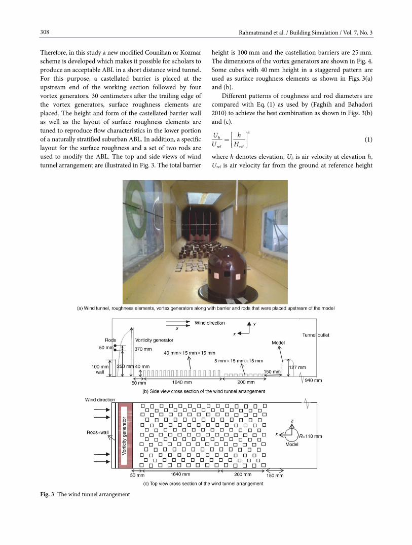
Therefore, in this study a new modified Counihan or Kozmar scheme is developed which makes it possible for scholars to produce an acceptable ABL in a short distance wind tunnel. For this purpose, a castellated barrier is placed at the upstream end of the working section followed by four vortex generators. 30 centimeters after the trailing edge of the vortex generators, surface roughness elements are placed. The height and form of the castellated barrier wall as well as the layout of surface roughness elements are tuned to reproduce flow characteristics in the lower portion of a naturally stratified suburban ABL. In addition, a specific layout for the surface roughness and a set of two rods are used to modify the ABL. The top and side views of wind tunnel arrangement are illustrated in Fig. 3. The total barrier

height is 100 mm and the castellation barriers are 25 mm. The dimensions of the vortex generators are shown in Fig. 4. Some cubes with 40 mm height in a staggered pattern are used as surface roughness elements as shown in Figs. 3(a) and (b).

Different patterns of roughness and rod diameters are compared with Eq. (1) as used by (Faghih and Bahadori 2010) to achieve the best combination as shown in Figs. 3(b) and (c).

ref ref

αhU h

U Hé ù

= ê úê úë û

(1)

where h denotes elevation, Uh is air velocity at elevation h, Uref is air velocity far from the ground at reference height

Fig. 3 The wind tunnel arrangement


309

Fig. 4 Design of vortex generators

Href and α is a constant which depends on the conditions of corresponding region. For the present measurements Uref

and Href are taken to be 15 m/s and 400 mm respectively. For the final pattern, a large number of exaggerated surface roughness elements (in a staggered pattern) as well as two rods with unique diameter of 10 mm (based on wind tunnel dimensions of 460 mm × 460 mm × 3260 mm) are utilized. This pattern reveals the fact that the height of elements along with the number of rods and their diameter are very important for producing an accurate ABL in a short distance of a small wind tunnel. In addition, the height of elements is decreased to 5 mm in the vicinity of the model, making it possible to maintain the form of velocity profile. Therefore, the model is just situated in 150 mm far from the elements, which is much far from the wake of elements of about 50 mm.

To present various flow characteristic, the origin of the coordinate is considered to be at the center of the building as shown in Fig. 3(c). The x axis is directed opposite to the flow while the y axis is directed upwards and z axis is in spanwise direction.

According to the produced ABL, a scale factor can be obtained. For this purpose, the roughness length parameter y0 according to (Cook 1978) should be determined. This is accomplished via fitting the measured mean velocity profile

to the logarithmic law of the wall. For the present design, the value of y0 found to be 1 mm. Satisfying the Jensen similarity (Je=h/y0), the scale factor will be about 1:100 for a territory with full-scale y0 = 10 cm in which the building is located.

The value of the required turbulent intensity is obtained by using full-scale data of ABL (ESDU 1985). The full-scale turbulence intensity for this kind of territory (in which the building is located) is between 15 and 20 percent (except in the vicinity of ground which is lower). This value of turbulence intensity is satisfied in the lower portion of the artificial ABL where the model is situated as shown in Fig. 5(a). This figure indicates that the turbulent intensity of the produced ABL is slightly less than that of the full-scale data. Matching of the mean velocity profile (α and y0), the turbulence intensities and Lxu cannot be achieved simul-taneously due to aperture limitation in the wind tunnel (Marshal 1975; Tieleman et al. 1978). Comparing flow pattern around a building and around its model in a wind tunnel, Marshal (1975) showed that inaccurate turbulence intensity simulation could lead to different value of fluctuation of various flow parameters (like pressure) in the model and full-scale building. Nevertheless, the difference is lower in the mean value of various flow parameters.

To ensure the uniformity of the produced ABL, the velocity profile should be compared at various locations of the wind tunnel. Figures 5(b) and (c) illustrate the velocity profile at various locations in both streamwise and cross streamwise directions. In Fig. 5(a), U10 is the velocity at an elevation of 10 m for a full-scale building. The measurements are started at about y1=2 mm above the tunnel wall due to the limitation of hot-wire size and displacement. The ratio of y1/Href is about 0.005 which is small compared to the plotting scale in Fig. 5. Therefore, we set zero as minimum scale in this figure. Velocity profiles are within the acceptable range for simulating ABL, as one compares with Eq. (1) for a suburban area.

In Fig. 5(b), the lower portion of the velocity profile at z=–50 mm exhibits a slight deviation from the desirable characteristics. This deviation may be attributed to the generated velocity profile and flow unsteadiness at such Reynolds number as well as wind tunnel inlet flow and distribution system. However, the velocity profile has less importance compared to the turbulence intensity and spectra of turbulence (Armitt and Counihan 1968). The measured turbulence spectrum shows proper agreement with other results as well as the design curves of ABL as shown in Fig. 6. In this figure fu is function FFT (fast Fourier’s transform), n is frequency, σ2

u is square of turbulence intensity and Lxu is longitudinal integral length scale of turbulence. One may notice fewer data points in the lower frequencies due to low accuracy of the present facilities. In the experiments,


310

Fig. 5 Comparison between velocity profiles and turbulent intensity at different locations of wind tunnel (the measurement is started from 2 mm above the ground)

Fig. 6 Variation of turbulence spectrum compared with other studies

distribution of Reynolds stress is also measured. It is found that the Reynolds stress of the full scale ABL is between 0.0 and 0.01 for the area of interest. A reasonable agreement is observed between the prototype and simulated model according to ESDU (1985) recommendation.

3 Experimental apparatus and measurements

Measurements are conducted in the open, blowing-type wind tunnel shown in Fig. 2. The tunnel is 3260 mm long and its cross section is 460 mm × 460 mm. Air speed in the tunnel can reach 25 m/s using a frequency inverter. The dome model used in this study has a height of 122 mm and a base diameter of 55 mm, giving a blockage ratio of around 6% in the tunnel. Flow Reynolds number based on the free stream velocity of 15 m/s and the height of the model, reaches 1.22×105. The experimental apparatus consists of hot wire probes, thermometer, constant temperature anemometer (CTA), A/D card, traversing system, PC and a monitoring device.

Experiments are carried out using a special dual sensor probe, capable of detecting flow reversal, fabricated by Fara Sanjesh Saba Co. (FSS). A single-sensor hot-wire probe is used for velocity measurements in the boundary layer flow outside the recirculation zone. To move the probe accurately in the tunnel, a three-dimensional, automatic traversing mechanism is installed. The dual-sensor probe has two parallel sensors; nickel film deposited on the quartz fiber. Calibration of each sensor is done in the tunnel using Karman-vortex technique (Schilichting and Gersten 2000). The calibration curves present a relationship between voltage and local velocity. Each calibration curve consists of a polynomial, converting voltage to velocity with a maximum deviation of 1%. For each test, the same incoming flow velocity is maintained by means of a pitot tube. Errors in


311

measuring the positions are limited to ±0.1 mm. Each set of measurements takes about 3 hours to conduct. During measurements, the average room temperature was about 19℃

with a fluctuation of ±1℃. The output of the constant temperature anemometer is affected by both velocity and the temperature difference between the wire and fluid. In order to measure the flow velocity accurately, the anemometer output has to be compensated for any variation of tem-perature during the measurements. In the present study, all anemometer bridge voltages were corrected based on a standard reference temperature of 27℃ by multiplying by a proper correction factor. Based on the measuring errors presented in Table 1, it is found that the uncertainties were 3% and 6.66% for velocity and turbulence intensity, respectively, determined according to Adams (1975). Some measurements are also repeated to ensure repeatability and the validity of the tested results.

To measure velocity components, u, v and turbulence intensity in two dimensions using a one-dimensional sensor, the method explained in Abdel-Rahman (1995) is adopted. The turbulence intensities obtained by this method, are compared with Klebanoff ’s results (Klebanoff and Tidstrom 1954). It is observed that the results found by this method have 10 to 15 percent difference.

Table 1 Ranges of measurement for various parameters and their uncertainties

Range Max. uncertainty

Free stream velocity 10 m/s –15 m/s 3%

Turbulence intensity 10% –20% 6.66%

4 Building the model

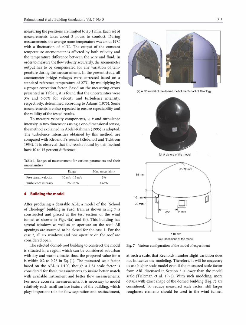
After producing a desirable ABL, a model of the “School of Theology” building in Yazd, Iran, as shown in Fig. 7 is constructed and placed at the test section of the wind tunnel as shown in Figs. 4(a) and (b). This building has several windows as well as an aperture on the roof. All openings are assumed to be closed for the case 1. For the case 2, all six windows and one aperture on the roof are considered open.

The selected domed-roof building to construct the model is situated in a region which can be considered suburban with dry and warm climate, thus, the proposed value for α is within 0.2 to 0.28 in Eq. (1). The measured scale factor based on the ABL is 1:100, though a 1:54 scale factor is considered for these measurements to insure better match with available instrument and better flow measurements. For more accurate measurements, it is necessary to model relatively each small surface feature of the building, which plays important role for flow separation and reattachment,

Fig. 7 Various configuration of the model of experiment

at such a scale, that Reynolds number slight variation does not influence the modeling. Therefore, it will be necessary to use higher scale model even if the measured scale factor from ABL discussed in Section 2 is lower than the model scale (Tieleman et al. 1978). With such modeling, more details with exact shape of the domed building (Fig. 7) are considered. To reduce measured scale factor, still larger roughness elements should be used in the wind tunnel,


312

which becomes impractical due to the limited distance between the vortex generator and the model (Tieleman et al. 1978).

For such arrangement, the blockage of the tunnel would be 6%, which considered reasonable (Tavakol et al. 2010). Based on such arrangement shown in Figs. 3 and 7, the building model occupied less than one third of the ABL, which is desirable for a part-depth simulation (Sharan 1977).

5 Results and discussions

5.1 Flow measurements

To illustrate the flow field, velocity distributions as well as turbulence intensity distributions are measured at various locations around the building for the two cases mentioned. The measured velocity distributions at symmetry plane of the building for cases 1 and 2 are shown in Figs. 8(a) and (b). (Case 1 pertains to the building with closed apertures

Fig. 8 Streamwise velocity distributions on the symmetry plane of domed building

and case 2 to the building with open apertures.) Velocity profile in front of the building is not affected significantly, and it follows the distribution of the ABL in both cases as seen in Figs. 5(b) and (c). On top of the dome, separation occurred at an angular position of 106 degrees for case 1, whereas it takes place at the tip of the roof for case 2 due to the open aperture, while Tavakol et al. (2010) reported the location of flow separation on a simple half-sphere at an angular position of 108 degrees.

A complex flow structure occurred behind the building. For case 1, due to specific shape of the roof, two large vortices are observed in the building’s wake as illustrated in Fig. 8(a) by dash lines. The lower portion of the building gives rise to the first one and the second one is due to the specific shape of the roof. For case 2, the openings add some disturbance to vortices, resulting in only one separation line in the symmetry plane, as shown in Fig. 8(b), whereas in Fig. 8(a) there are two separation lines. The presented result indicates that, these vortices gradually disappeared downstream of the building and a reattachment zone is formed. For case 1 (Figs. 7(b) and (c)), on the roof, the streamlines bend towards the symmetry plane and con-sequently two separation lines are formed on the symmetry plane, whereas for case 2, the airflow passing through the windows and aperture on the roof alters this effect, leading to only one separation line on the symmetry plane.

Besides, with a quick comparison of Figs. 8(a) and (b), one may anticipate that opening the windows contributes to the increase of the wake’s length and a more complex flow, since in case 2 the slope of the wake region is less than that in case 1. These windows allow the entrance of high momentum fluid into the building’s wake resulting in a longer wake behind the building. Furthermore, observing Figs. 8(a) and (b), one may conclude that in both cases, on the roof, the height of the building’s wake is almost as high as the building. Nevertheless, in case 2, this height is slightly higher due to the open aperture on the roof. The same results were obtained by Tavakol et al. (2010) for half of a hemisphere placed on a wind tunnel floor. The height of the wake region is decreased with a slighter slope for both cases 1 and 2 compared to that of (Tavakol et al. 2010) due to the fact that the building height above the floor is higher than that of a simple half-sphere.

The maximum value of reversed flow occurs in case 1 on the top of the roof with a magnitude of about 11 m/s. The reason rests on the fact that in case 2, a portion of airflow passes through the windows. Therefore, the momentum of airflow passing over the roof decreases with respect to case 1. In addition, in case 2, the upward flow exhausted from the aperture in the roof leads to a strong disturbance in the flow field, resulting in less intense reversed flow at this region.


313

In a same manner, the maximum value of reversed flow at the building’s wake region occurs in case 1 (which is 5 m/s). The reason is that the airflows passing through the rear windows in case 2 leads to decreasing the value of reversed flow behind the building. Moreover, due to effect of specific shape of the roof and apex of the building, the value of reversed flow on top of the roof is more than that behind the building in both cases 1 and 2.

Turbulence intensity along the symmetry plane is shown in Figs. 9(a) and (b). In both cases, the intensity decreases gradually in x direction behind the model. Behind the model, maximum intensity occurs in an elevation of 3/5H. It is approximately 60 percent higher than the maximum intensity of the ABL in the same height. On top of the roof, maximum intensity occurs near the roof apex, which is the maximum value in the whole flow field. At front, the intensity of turbulence follows the same trend as the ABL. According to this trend, turbulent intensity increases by

Fig. 9 Streamwise turbulence intensity distributions on the symmetry plane of domed building

elevation, then, at a specified elevation, it starts to decrease with the same trend as that of the full-scale ABL. Trends are similar behind the building and top of the roof except for a more intense peak in the locations of maximum intensity for all lines shown in Figs. 9(a) and (b). This trend reveals the fact that the maximum turbulent intensity in different locations in x direction occurs at the edge of shear flow region (Tavakol et al. 2010) as shown with dash lines in Figs. 9(a) and (b).

Such flow structures in a building with open windows like the one for case 2 will affect ventilation of the building and thermal exchange between the roof surface and ambient air during hot summer days. Due to some limitations in moving hot wire probe inside the building, it is not possible to measure the flow field inside the building to show this effect. Therefore, numerical simulation is performed for the arrangement shown in Fig. 7 for the model with open apertures to illustrate the mentioned effect on ventilation of the building.

5.2 Numerical calculations

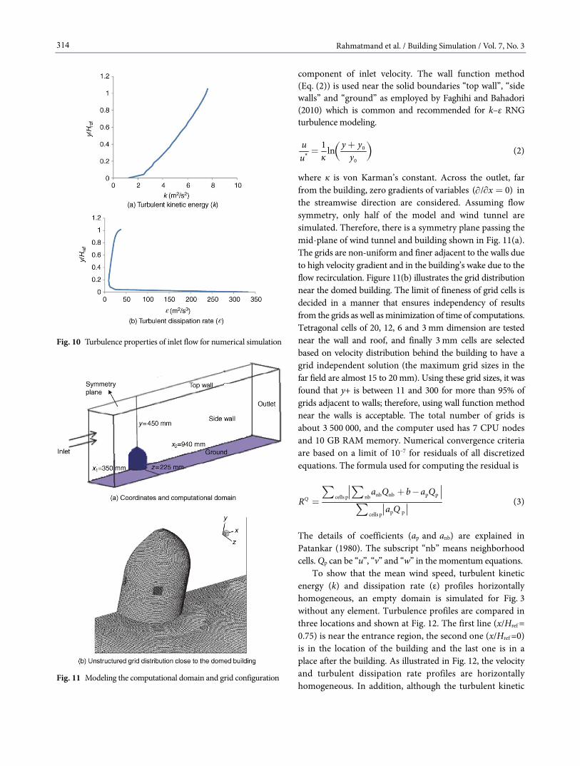
In addition to experimental measurements, an available discretized CFD code in the high computational center of Mechanical Engineering Department of Shiraz University (Tavakol et al. 2010; Hadavand and Yaghoubi 2008) is utilized to solve the governing equations in the computational domain using finite volume method. For the present study, upwind scheme is used for discretization along with SIMPLE algorithm for pressure–velocity coupling and RNG k–ε model for turbulence modeling, as described in (Hadavand and Yaghoubi 2008). The computational domain consists of a single fluid block. The domain size is equal to the wind tunnel dimension. Inlet velocity profile is taken from Eq. (1) with α=0.28 which is in line with the measurements as shown in Fig. 5(b). Moreover, an additional simulation is performed for the upstream part of tunnel in the wind tunnel (rough surface). The average size of roughness elements are considered for numerical simulation of rough surface, and the inlet profiles is considered uniform for this part, to have the same condition as the inlet part of wind tunnel. Moreover, to have more realistic inlet condition in the computational main domain, the corresponding turbulence profiles after the roughness elements (at the end of first part of simulation) are assumed as inlet in the main computational domain. The inlet turbulence profiles for the main computational domain are shown in Fig. 10 up to four times of building’s height.

The computational domain is shown in Fig. 11(a) along with its attributed dimensions. According to Fig. 11(a), an appropriate profile (Eq. (1)) is incorporated for the x


314

Fig. 10 Turbulence properties of inlet flow for numerical simulation

Fig. 11 Modeling the computational domain and grid configuration

component of inlet velocity. The wall function method (Eq. (2)) is used near the solid boundaries “top wall”, “side walls” and “ground” as employed by Faghihi and Bahadori (2010) which is common and recommended for k–ε RNG turbulence modeling.

*0

0

1 ln y yuκ yu

+= ( ) (2)

where к is von Karman’s constant. Across the outlet, far from the building, zero gradients of variables ( / 0)x = in the streamwise direction are considered. Assuming flow symmetry, only half of the model and wind tunnel are simulated. Therefore, there is a symmetry plane passing the mid-plane of wind tunnel and building shown in Fig. 11(a). The grids are non-uniform and finer adjacent to the walls due to high velocity gradient and in the building’s wake due to the flow recirculation. Figure 11(b) illustrates the grid distribution near the domed building. The limit of fineness of grid cells is decided in a manner that ensures independency of results from the grids as well as minimization of time of computations. Tetragonal cells of 20, 12, 6 and 3 mm dimension are tested near the wall and roof, and finally 3 mm cells are selected based on velocity distribution behind the building to have a grid independent solution (the maximum grid sizes in the far field are almost 15 to 20 mm). Using these grid sizes, it was found that y+ is between 11 and 300 for more than 95% of grids adjacent to walls; therefore, using wall function method near the walls is acceptable. The total number of grids is about 3 500 000, and the computer used has 7 CPU nodes and 10 GB RAM memory. Numerical convergence criteria are based on a limit of 10–7 for residuals of all discretized equations. The formula used for computing the residual is

nb nb p pcells p nb

p pcells p

Qa Q b a Q

Ra Q

+ -=å å

å (3)

The details of coefficients (ap and anb) are explained in Patankar (1980). The subscript “nb” means neighborhood cells. Qp can be “u”, “v” and “w” in the momentum equations.

To show that the mean wind speed, turbulent kinetic energy (k) and dissipation rate (ε) profiles horizontally homogeneous, an empty domain is simulated for Fig. 3 without any element. Turbulence profiles are compared in three locations and shown at Fig. 12. The first line (x/Href = 0.75) is near the entrance region, the second one (x/Href =0) is in the location of the building and the last one is in a place after the building. As illustrated in Fig. 12, the velocity and turbulent dissipation rate profiles are horizontally homogeneous. In addition, although the turbulent kinetic


315

Fig. 12 Mean velocity and turbulence properties in an empty domain

energy profile has a slight difference at entrance region and building location, there is a partially agreement between them at least up to the three times of building’s height. It should be added that the gradient of “k” can be held responsible at least partially to have a reasonable simulation

of ABL (Blocken et al. 2007). To validate the numerical code and the corresponding

turbulence model for such junction flow, results of flow over step geometry, as explained by Hadavand and Yaghoubi (2008), are determined. This sort of geometry is widely used to assess turbulence models for predicting flow separation. The length of the reversed flow region is in the range between 6.5H and 7.5H where in the present work it was found to be 6.94H. This verifies the numerical code and the RNG k–ε turbulence model used for the numerical calculations.

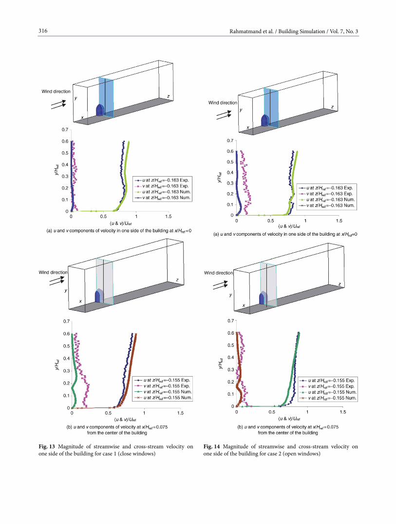
Assuming symmetry of flow field, for x/Href >0.0, the experimental and numerical values of u and v components of velocity for locations in the vicinity of the building are compared in Figs. 13 and 14 for both cases 1 and 2. In both cases, the u component is lower near the ground and increases gradually upward. On the other hand, v component decreases gradually with elevation. From Figs. 13 and 14, one may conclude that decreasing the building’s width leads to the increase of u component and the decrease of v components by elevation.

Comparing Figs. 13(a) and (b) shows that despite the non-zero value of the v component at x/Href =0.075, there is almost no two-dimensional flow for location of x/Href =0 due to symmetry of building at this plane, as expected. The rise of v values in Fig. 14(a) at x/Href =0 with respect to Fig. 13(a) is due to the outflow or inflow of air from windows which leads to a more complex flow field.

There are slight differences between numerical and experimental results in Figs. 13 and 14. The difference is more obvious for the v component, but, according to the accuracy of two-dimensional measurements, this might be considered acceptable, since the order of v component is about 0.1 m/s, which is almost close to the accuracy of experimental measurements.

According to the numerical simulation, the apertures in the windward side have the maximum fresh air inlet flow rate, and the windows on the opposite side have the maximum outlet flow rate. Due to these streams through windows, a complex flow structure is developed which is a mixture of various streams.

Comparing numerical computations with experimental measurements, proper compatibility is observed in Fig. 15 for velocity profile at various sections. However, there is a difference between calculated and measured velocity profiles behind the building, which may encourage us to use LES method or some similar methods to diminish this difference. Figure 16 presents the flow field inside, outside and around the building. Air enters the building from the forward opening and gives rise to considerable ventilation, which is desirable to provide thermal comfort conditions during moderate outdoor temperatures.


316

Fig. 13 Magnitude of streamwise and cross-stream velocity on one side of the building for case 1 (close windows)

Fig. 14 Magnitude of streamwise and cross-stream velocity on one side of the building for case 2 (open windows)


317

Fig. 15 Comparison of velocity profile for various sections along the mid-plane

Fig. 16 Pattern of streamlines on different planes in streamwise direction

To demonstrate the effect of airflow through windows and roof aperture, iso-surfaces of constant vorticity ωx and ωz are illustrated in Fig. 17. This figure shows that, airflow is exhausted in a spiraling motion from the side windows.

Fig. 17 Iso-surfaces of constant ωx and ωz outside and inside the domed building


318

This exhausting airflow not only affects horseshoe vortex and the flow pattern around the building, but it leads to appropriate ventilation for the building. However, more interesting is the effect of these openings on the flow field inside the building. As illustrated in Fig. 17, some vortices in different directions formed inside the building. From Fig. 17(c), two large vortices exist in the center of the building (due to the windows effect) and in the region below the roof (due to the roof aperture effect) as well as a secondary flow in the bottom corner of the building which are important patterns, as the habitants usually rest in these areas. It is clear that this pattern leads to proper mixing and swirling of air inside the building. Such flow pattern makes suitable ventilation inside the building. Nevertheless, it should be noted that, for obtaining more accurate flow structure around the building, more advanced turbulence- modeling (like LES or direct numerical simulation methods) along with more accurate boundary condition measurements are needed to be applied.

In addition, using numerical results, the air discharge coefficient, which is necessary for assessing the ventilation rate of a building, is determined by Eq. (4):

z 2ΔρC u

p= (4)

where, u is the average air velocity (m/s) passing through the window, ρ is air density (kg/m3) and Δp is a measure of the static pressure difference across the opening (Pa). For the domed-roof building shown in Fig. 7(a), for the windward window, the value of Cz is found to be 0.68 which is in line with the results presented in Chiu and Etheridge (2007). Consequently, if the traditional design architecture could be utilized, it would be possible to provide a suitable comfort situation along with energy-saving. This effect is dominant for summer time, especially in the morning and late afternoon, when ambient air temperature is around 28–30℃ and relative humidity is low.

6 Conclusions

In this study, attempt is made to produce atmospheric boundary layer and measure turbulent airflow around a domed-roof building. The results show that: (1) For a small wind tunnel, using the proposed method, the

atmospheric boundary layer can be developed within a small length, which can be used as a tool for environmental studies.

(2) For the domed-roof building studied, two vortices behind the building are observed for closed apertures: while for open windows, one recirculation can be seen behind the building. For the building with open windows, the

airflow through openings leads to more disturbances and mixing of the adjacent flows.

(3) Maximum turbulence intensity occurred on the edge of the shear flow along the mid symmetry plane. Also, the value of maximum turbulence intensity on the roof is higher than elsewhere due to vertical flow exhausting the aperture on the roof, whereas airflow passing through the back windows of the building in streamwise direction does not cause the same effect.

(4) The flow separation occurred at an angular position of 106° on the roof for closed roof aperture (case 1). For open aperture on the roof (which enhances ventilation), it occurred on the location of the hole (case 2).

Acknowledgements

The authors appreciate support from Iran’s National Elite Foundation.

References

Abdel-Rahman AA (1995). On the yaw angle characteristics of hot-wire anemometer. Flow Measurement and Instrumentation, 6: 271–278.

Adams IF (1975). Engineering Measurements and Instrumentation. London: English University Press.

Armitt J, Counihan J (1968). The simulation of the atmospheric boundary layer in a wind tunnel. Atmospheric Environment, 2: 49–71.

Asfour OS, Gadi MB (2008). Using CFD to investigation ventilation characteristics of vaults as wind-inducing devices in building. Applied Energy, 85: 1126–1140.

Bahadori MN (1978). Passive cooling systems in Iranian architecture. Scientific America, 238: 144–154.

Blocken B, Stathopoulos T, Carmeliet J (2007). CFD simulation of the atmospheric boundary layer: Wall function problems. Atmospheric Environment, 41: 238–252.

Chiu Y-H, Etheridge DW (2007). External flow effects on the discharge coefficients of two types of ventilation opening. Journal of Wind Engineering and Industrial Aerodynamics, 95: 225–252.

Cook NJ (1978). Determination of the model scale factor in wind tunnel simulations of the adiabatic atmospheric boundary layer. Journal of Wind Engineering and Industrial Aerodynamics, 2: 311–321.

De Bortoli ME, Natalini B, Paluch MJ, Natalini MB (2002). Part-depth wind tunnel simulations of the atmospheric boundary layer. Journal of Wind Engineering and Industrial Aerodynamics, 90: 281–291.

ESDU 85020 (1985). Characteristics of atmospheric turbulence near the ground: Strong winds (neutral atmosphere). Engineering Sciences Data Unit 85020.

Faghih AK, Bahadori MN (2010). Three dimensional numerical investigation of air flow over domed roofs. Journal of Wind Engineering and Industrial Aerodynamics, 98: 161–168.

Hadavand M, Yaghoubi M (2008). Thermal behavior of curved roof


319

buildings exposed to solar radiation and wind flow for various orientations. Applied Energy, 85: 663–679.

Harris RI (1968). Measurements of wind structure at heights up to 598 ft. above ground level. In: Proceedings of Symposium Wind Effects on Buildings and Structures. Loughborough University, UK.

Klebanoff PS, Tidstrom KD (1954). Characteristics of turbulence in a boundary-layer with zero pressure gradient. NACA Technical note; No. 3178.

Kozmar H (2011). Truncated vortex generators for part-depth wind- tunnel simulations of the atmospheric boundary layer flow. Journal of Wind Engineering and Industrial Aerodynamics, 99: 130–136.

Maher FJ (1965). Wind load on basic dome shapes. Journal of the Structural Division, ASCE, 91, ST3: 219–228.

Mainstone RJ (1983). Developments in Structural Form. Cambridge, USA: MIT Press.

Marshal RD (1975). A study of wind pressures on a single family dwelling in model and full scale. Journal of Wind Engineering and Industrial Aerodynamics, 1: 177–199.

Owen PR, Zienkiewicz HK (1957). The production of uniform shear flow in a wind tunnel. Journal of Fluid Mechanics, 2: 521–531.

Patankar SV (1980). Numerical Heat Transfer and Fluid Flow. Bristol, USA: Hemisphere Publishing, pp. 120–130.

Prajongsan P, Sharples S (2012). Enhancing natural ventilation, thermal comfort and energy savings in high-rise residential buildings in Bangkok through the use of ventilation shafts. Building and Environment, 50: 104–113.

Savory E, Toy N (1968). The flow regime in the turbulent near wake of a hemisphere. Experiments in Fluids, 4: 181–188.

Schilichting H, Gersten K (2000). Boundary-Layer Theory. Berlin: Springer, Chapter 2.

Schon JP, Mery P (1967). A preliminary study of the simulation of neutral atmospheric boundary layer using air injection in a wind tunnel. Atmospheric Environment, 5: 299–311.

Sharan V (1977). On the influence of the characteristics of flow on pressure distribution around building models with a view to simulating the minimum height of the atmospheric boundary layer. International Journal of Mechanical Sciences, 19: 379-387.

Sluman TJ, van Maanen HR, Ooms G (1980). Atmospheric boundary layer simulation in a wind tunnel, using air injection. Applied Scientific Research, 36: 289–307.

Tavakol MM, Yaghoubi M, Masoudi Motlagh M (2010). Air flow aerodynamic on a wall-mounted hemisphere for various turbulent boundary layers. Experimental Thermal and Fluid Science, 34: 538–553.

Tieleman HW, Reinhold TA, Marshal RD (1978). On the wind-tunnel simulation of the atmospheric surface layer for the study of wind loads on low-rise buildings. Journal of Wind Engineering and Industrial Aerodynamics, 3: 21–38.

Wier M, Römer L (1987). Experimentelle untersuchung von stabil und instabil geschichteten turbulenten plattengrenzschichten mit bodenrauhigkeit. Zeitschrift fur Flugwissenschaften und Weltraumforschung, 11: 78–86. (in German)

3d experimental and numerical analysis of wind flow around domed-roof buildings with open and closed...

Documents