361: 17 curves and surfaces - simon fraser universitytorsten/teaching/cmpt361/lecture... · •...
TRANSCRIPT
© Machiraju/Zhang/Möller© Machiraju/Zhang/Möller
Curves and Surfaces
CMPT 361Introduction to Computer Graphics
Torsten Möller
© Machiraju/Zhang/Möller
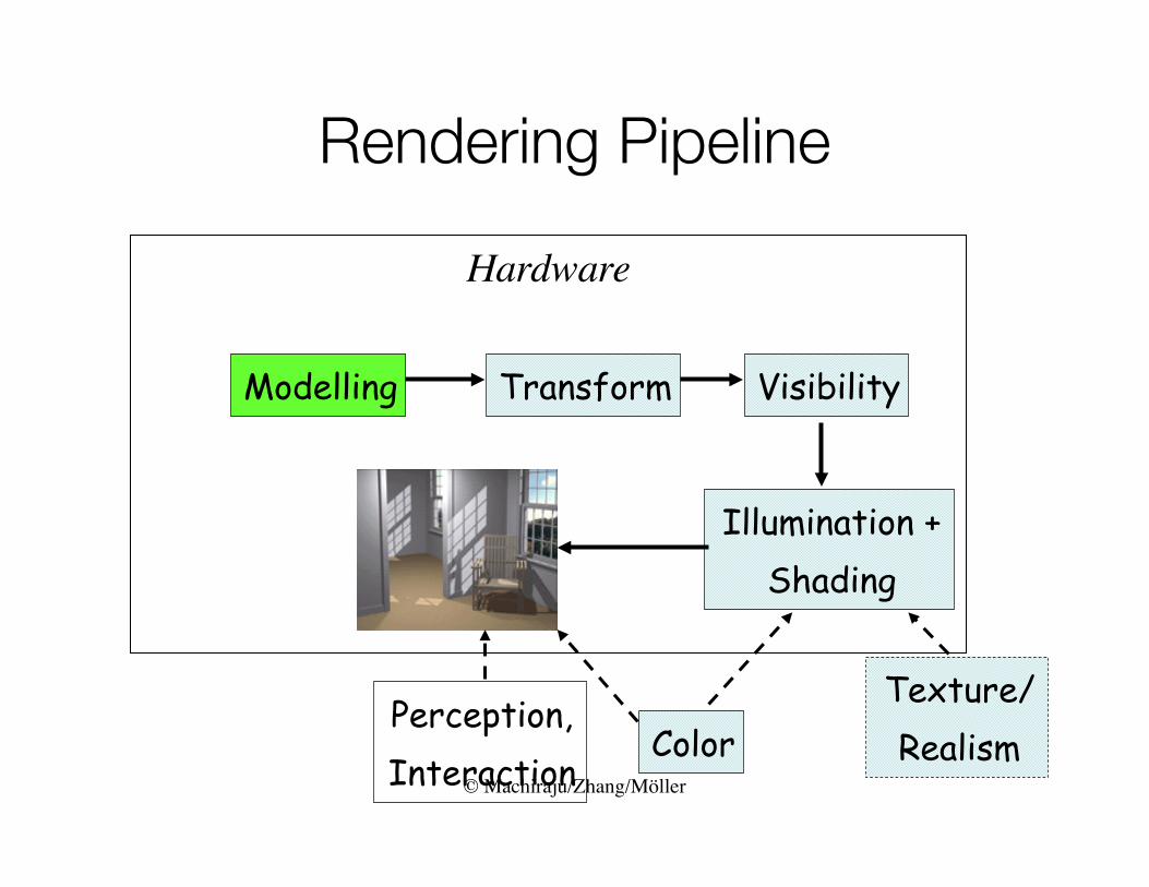
Rendering Pipeline
Hardware
Modelling Transform Visibility
Illumination +Shading
ColorPerception,Interaction
Texture/Realism

© Machiraju/Zhang/Möller
Reading• Angel – Chapter 10• Foley et al. - Chapter 11
3

© Machiraju/Zhang/Möller
Today• Polynomials• Parametric representation• Fairness vs. smoothness• Parametric vs. geometric continuity• Hermite spline• Bezier spline• B-Spline• Surfaces• Subdivision 4

© Machiraju/Zhang/Möller [Zorin 01]
Filling a gap …• So far, we have focused on lines, flat
polygons, and simple objects, e.g., spheres• Missing: freeform curves and surfaces• Although smooth curves and surfaces are
converted to polygonal curves and meshes when rendered, they still provide a good option for modeling
• We follow the text loosely
5

© Machiraju/Zhang/Möller
Why curves and surfaces?• Natural to use for modeling of smooth shapes,
e.g., – Body of an automobile– Shape of cartoon characters (Shrek)– Motion curves in animation, etc.
• Smoothness can often be guaranteed analytically
• Compact (analytical) representation• Theory of smooth curves and surfaces, e.g.,
from calculus and differential geometry, is well-developed 6
http://www.shrek2.com/

© Machiraju/Zhang/Möller
Polynomial curves and surfaces• In computer graphics, we prefer curves and
surfaces represented by polynomials– Approximation power: Can approximate any
continuous function to any accuracy (Weierstrass’s Theorem)
– Can offer local control for shape design through the use of piecewise polynomials
– All derivatives and integrals are available (infinitely smooth) and easy to compute
– Compact representation– Efficient evaluation – e.g., Horner’s rule 7
© Machiraju/Zhang/Möller
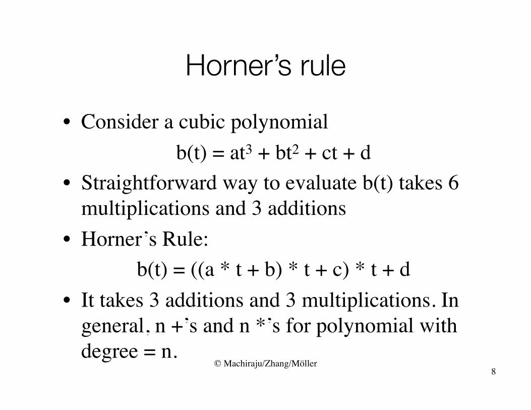
Horner’s rule• Consider a cubic polynomial
b(t) = at3 + bt2 + ct + d• Straightforward way to evaluate b(t) takes 6
multiplications and 3 additions• Horner’s Rule:
b(t) = ((a * t + b) * t + c) * t + d• It takes 3 additions and 3 multiplications. In
general, n +’s and n *’s for polynomial with degree = n.
8

© Machiraju/Zhang/Möller
Curve & surface representation• Explicit: y = f(x), z = f(x, y)• Implicit (level-set): f(x,y) = 0, f(x, y, z) = 0• Parametric:
– 2D planar curve segment: (x(t), y(t)), t ∈[0, 1]
– 3D space curve segment: (x(t), y(t), z(t)), t ∈[0, 1]
– 3D parametric surface patch: (x(u, v), y(u, v), z(u, v)), u, v ∈[0, 1]
9

© Machiraju/Zhang/Möller
Basis Functions
http://terpconnect.umd.edu/~petersd/interp.html
10
© Machiraju/Zhang/Möller
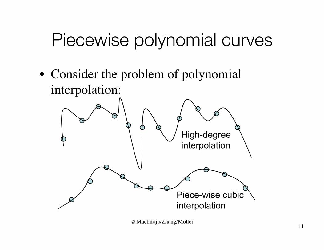
Piecewise polynomial curves• Consider the problem of polynomial
interpolation:
11
High-degree interpolation
Piece-wise cubic interpolation
© Machiraju/Zhang/Möller
Today• Polynomials• Parametric representation• Fairness vs. smoothness• Parametric vs. geometric continuity• Hermite spline• Bezier spline• B-Spline• Surfaces• Subdivision 12
© Machiraju/Zhang/Möller
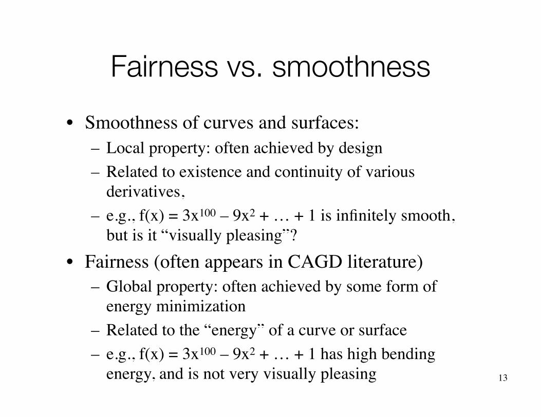
Fairness vs. smoothness• Smoothness of curves and surfaces:
– Local property: often achieved by design– Related to existence and continuity of various
derivatives,– e.g., f(x) = 3x100 – 9x2 + … + 1 is infinitely smooth,
but is it “visually pleasing”?• Fairness (often appears in CAGD literature)
– Global property: often achieved by some form of energy minimization
– Related to the “energy” of a curve or surface– e.g., f(x) = 3x100 – 9x2 + … + 1 has high bending
energy, and is not very visually pleasing 13

© Machiraju/Zhang/Möller
Parametric cubic curves• Let us focus on parametric curves for now• Generalization to surfaces is quite straightforward• Questions: what degree (of the polynomials) to
use?– Degree 0 – 2 (constant, linear, or quadratic): often has
too little flexibility– High-degree: unnecessarily complex and easy to
introduce undesirable wiggles (most objects we want to model using curves and surfaces are somewhat fair) – fairness vs. smoothness
– Most commonly used in graphics: parametric cubic (degree-3) curves and surfaces 14
© Machiraju/Zhang/Möller
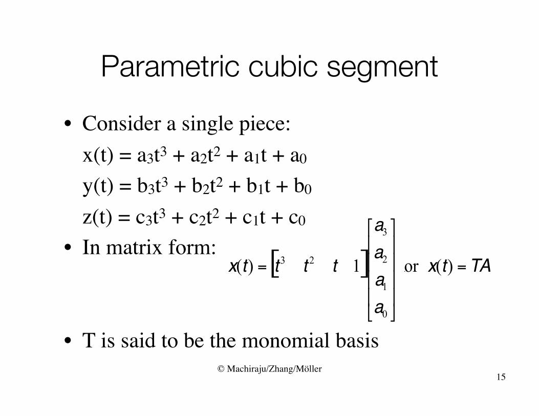
Parametric cubic segment• Consider a single piece:
x(t) = a3t3 + a2t2 + a1t + a0
y(t) = b3t3 + b2t2 + b1t + b0
z(t) = c3t3 + c2t2 + c1t + c0
• In matrix form:
• T is said to be the monomial basis15

© Machiraju/Zhang/Möller
Derivatives and continuity• 1st-order derivative of (x(t), y(t)): (x’(t), y’(t)) –
tangent
• 2nd-order derivative: (x’’(t), y’’(t)) – related to curvature
• Parametric continuity of a curve (smoothness of motion):– C0 continuous: curve is joined or connected– C1: requires C0 & 1st-order derivative is continuous– C2: requires C0 & C1 & 2nd-order derivative is cont.– Cn: requires C0 & … & Cn–1 & nth derivative cont. 16
© Machiraju/Zhang/Möller
Continuity of piecewise polynomials
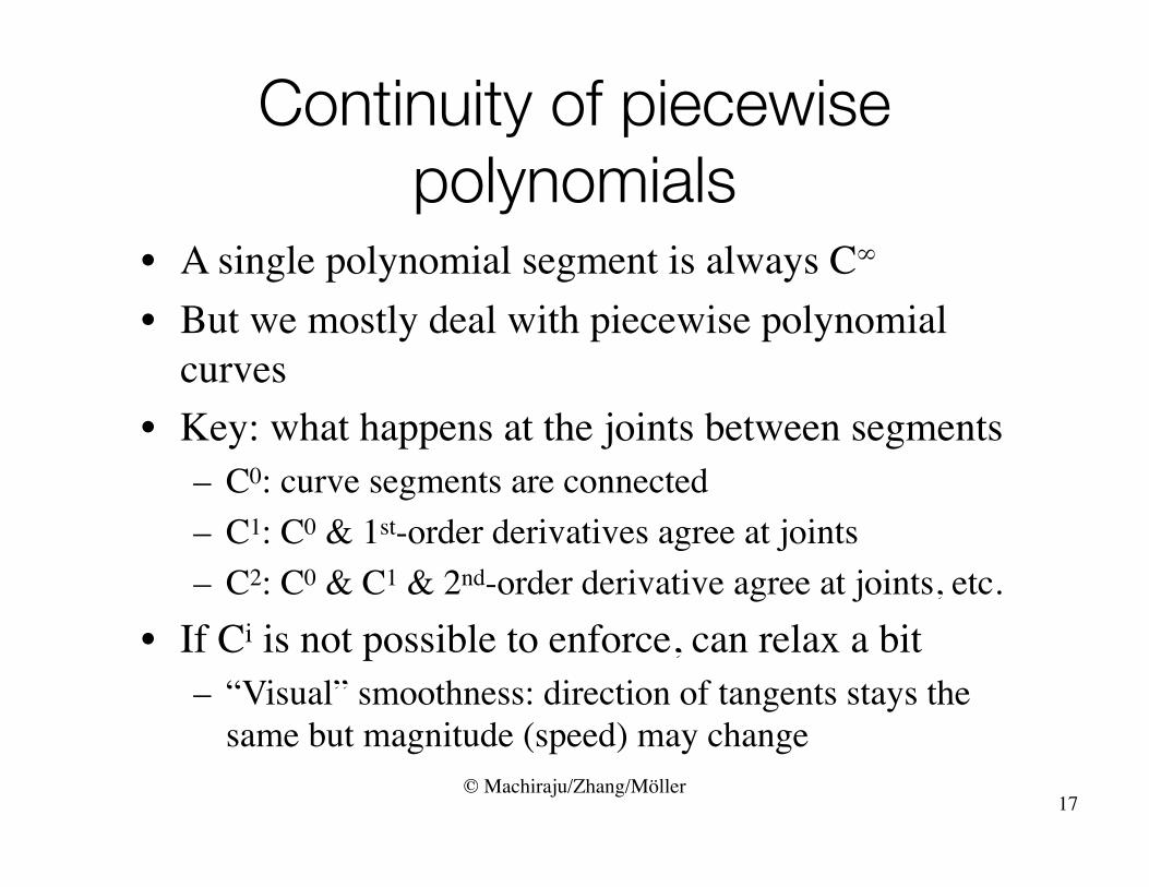
• A single polynomial segment is always C∞ • But we mostly deal with piecewise polynomial
curves• Key: what happens at the joints between segments
– C0: curve segments are connected– C1: C0 & 1st-order derivatives agree at joints– C2: C0 & C1 & 2nd-order derivative agree at joints, etc.
• If Ci is not possible to enforce, can relax a bit– “Visual” smoothness: direction of tangents stays the
same but magnitude (speed) may change
17
© Machiraju/Zhang/Möller
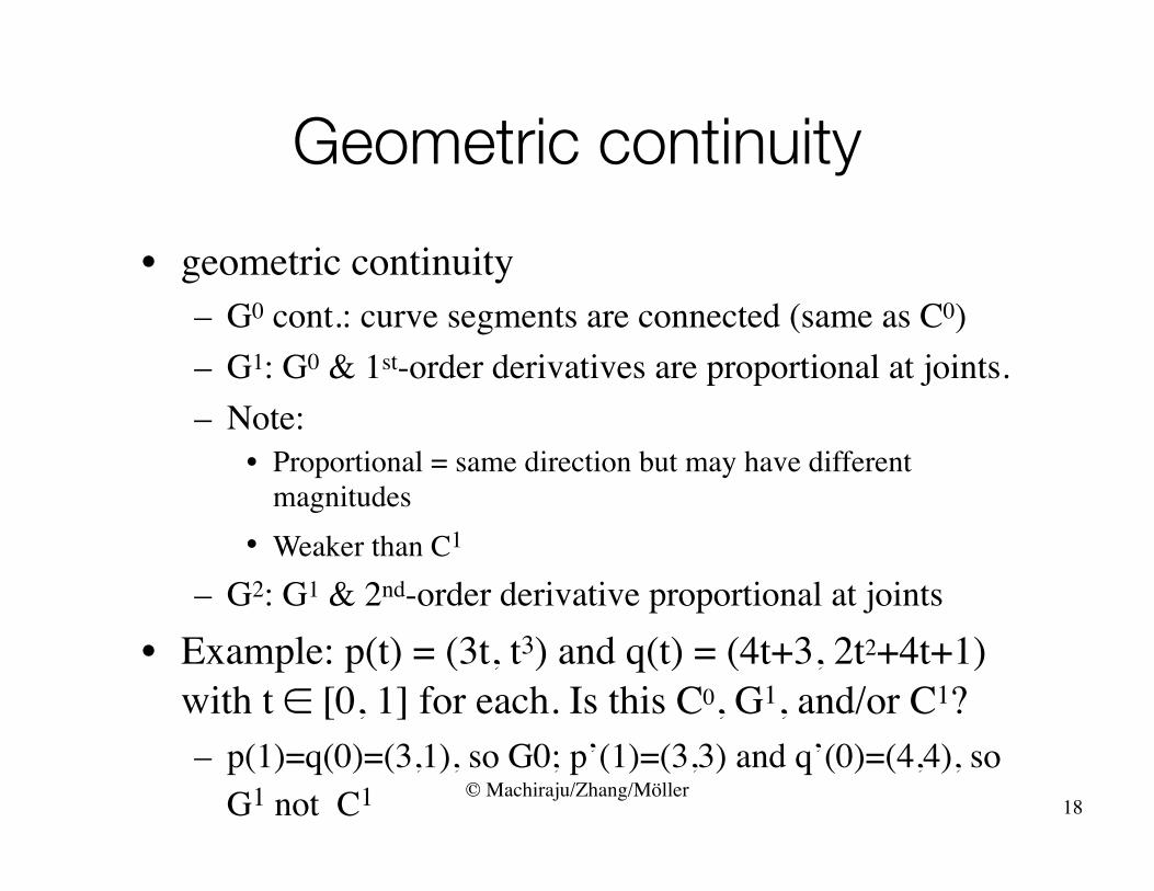
Geometric continuity• geometric continuity
– G0 cont.: curve segments are connected (same as C0)– G1: G0 & 1st-order derivatives are proportional at joints. – Note:
• Proportional = same direction but may have different magnitudes
• Weaker than C1
– G2: G1 & 2nd-order derivative proportional at joints• Example: p(t) = (3t, t3) and q(t) = (4t+3, 2t2+4t+1)
with t ∈ [0, 1] for each. Is this C0, G1, and/or C1?– p(1)=q(0)=(3,1), so G0; p’(1)=(3,3) and q’(0)=(4,4), so
G1 not C1 18

© Machiraju/Zhang/Möller
On to curve design• We want to design piecewise cubic polynomial curves
that satisfy certain design constraints, e.g.,– Curve should pass through certain points– Curve should have some given derivatives at specific points– Curve should be smooth: G1, C1, C2, or …– Curve must be contained in certain area, or has at most this
length, etc.• Need proper basis functions to facilitate design process• These basis functions or blending functions blend
together the individual contributions of the control points
19
© Machiraju/Zhang/Möller
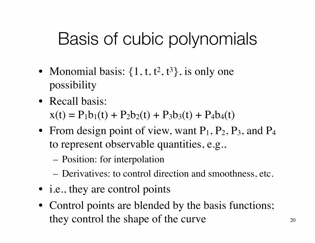
Basis of cubic polynomials• Monomial basis: {1, t, t2, t3}, is only one
possibility • Recall basis:
x(t) = P1b1(t) + P2b2(t) + P3b3(t) + P4b4(t)• From design point of view, want P1, P2, P3, and P4
to represent observable quantities, e.g.,– Position: for interpolation– Derivatives: to control direction and smoothness, etc.
• i.e., they are control points• Control points are blended by the basis functions;
they control the shape of the curve 20

© Machiraju/Zhang/Möller
Ex. 1: Hermite curves• Defined by two points (P1 and P4) and two
tangents (R1 and R4)• Aim: Achieve C1 or G1 continuity• Want cubic curve x(t),
t ∈ [0, 1], such that (y and z are similar)– x(0) = P1
– x(1) = P4
– x’(0) = R1
– x’(1) = R4 21
Let us note that the control “points” P1, P4, R1, and R4 are all observable quantities and they control the shape of the curve
R1
R4
P4
P1

© Machiraju/Zhang/Möller
Cubic Hermite curves• x(t) = TA = a3t3 + a2t2 + a1t + a0, where T =
[t3 t2 t 1] and A = [a3 a2 a1 a0]T. We want
• So G = BA and thus A = B–1G• It follows that x(t) = TA = TB–1G = HG
22
© Machiraju/Zhang/Möller
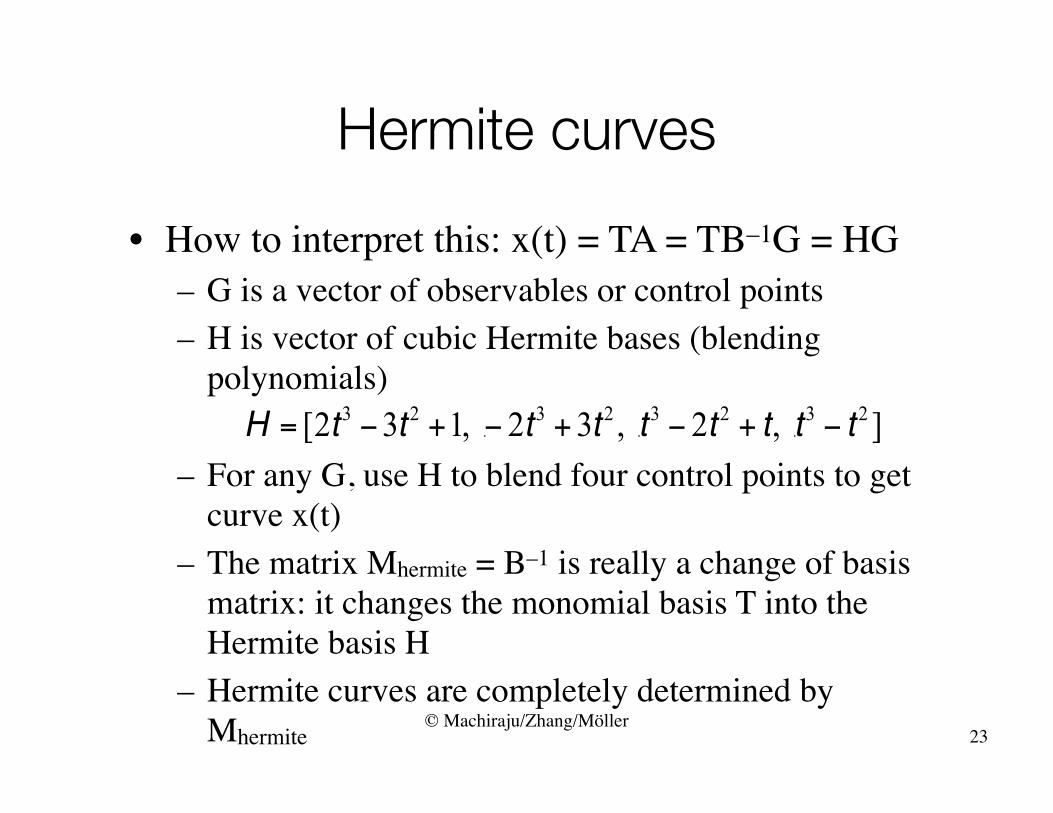
Hermite curves• How to interpret this: x(t) = TA = TB–1G = HG
– G is a vector of observables or control points– H is vector of cubic Hermite bases (blending
polynomials)
– For any G, use H to blend four control points to get curve x(t)
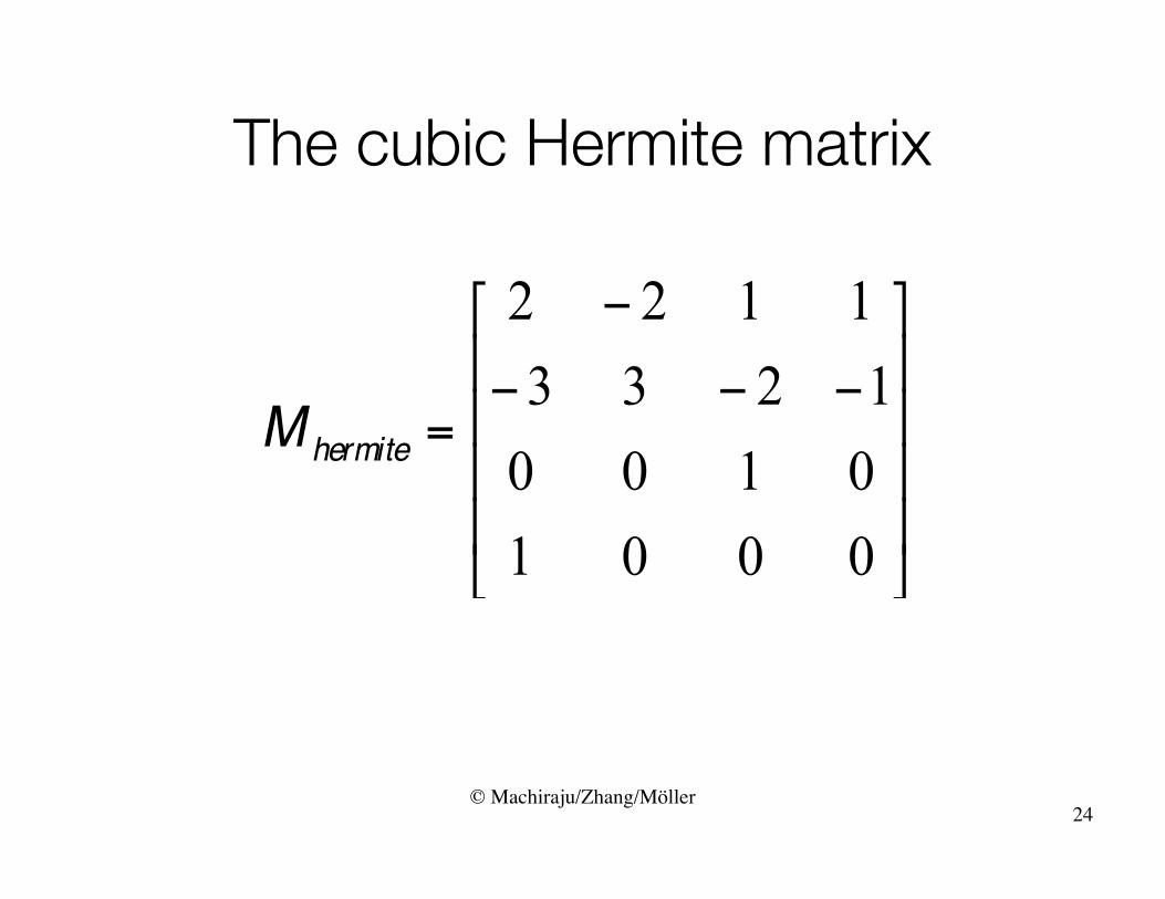
– The matrix Mhermite = B–1 is really a change of basis matrix: it changes the monomial basis T into the Hermite basis H
– Hermite curves are completely determined by Mhermite 23
© Machiraju/Zhang/Möller
The cubic Hermite matrix
24

© Machiraju/Zhang/Möller
Piecewise Hermite curves• Can obviously enforce C1 or G1 continuity
at the joints
• Each segment parameterized over [0, 1], as usual
25
R1
R4 = kR’1
P4 = P’1
P1
P’4
R’4

© Machiraju/Zhang/Möller
Today• Polynomials• Parametric representation• Fairness vs. smoothness• Parametric vs. geometric continuity• Hermite spline• Bezier spline• B-Spline• Surfaces• Subdivision 26

© Machiraju/Zhang/Möller
Ex. 2: Cubic Bézier curve• Defined by four control points P0, P1, P2, and P3
– x(0) = P0
– x(1) = P3
– x’(0) = 3(P1 – P0)– x’(1) = 3(P3 – P2)
• Convex hull property: Bézier curve lies within the convex hull of the four control points – good control
• Convex hull of a set of points on the plane: tightest convex polygon enclosing the set
27
© Machiraju/Zhang/Möller
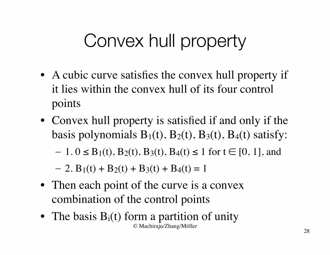
Convex hull property• A cubic curve satisfies the convex hull property if
it lies within the convex hull of its four control points
• Convex hull property is satisfied if and only if the basis polynomials B1(t), B2(t), B3(t), B4(t) satisfy:– 1. 0 ≤ B1(t), B2(t), B3(t), B4(t) ≤ 1 for t ∈ [0, 1], and– 2. B1(t) + B2(t) + B3(t) + B4(t) = 1
• Then each point of the curve is a convex combination of the control points
• The basis Bi(t) form a partition of unity28
© Machiraju/Zhang/Möller
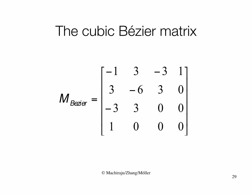
The cubic Bézier matrix
29

– B0(t) = (1 – t)3, B1(t) = 3t(1 – t)2, – B2(t) = 3t2(1 – t), B3(t) = t3
• Well known as the Bernstein Polynomials of degree 3
• Bernstein polynomials of degree n• We have• Partition of unity easy to see: Σi Bi(t) = [t + (1 – t)]n
© Machiraju/Zhang/Möller
Bézier basis polynomials
30
© Machiraju/Zhang/Möller
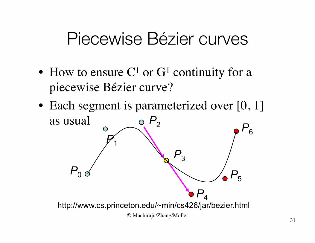
Piecewise Bézier curves• How to ensure C1 or G1 continuity for a
piecewise Bézier curve?• Each segment is parameterized over [0, 1]
as usual
http://www.cs.princeton.edu/~min/cs426/jar/bezier.html
31
P0
P1
P2
P3
P4
P5
P6

© Machiraju/Zhang/Möller
Ex 3. Cubic B-Spline curves• Most popular choice in computer graphics• They are C2 continuous – this beats Hermite
and Bézier curves in terms of smoothness• The theory of B-splines is very rich• NURBS: nonuniform rational B-splines
– Each component is rational: x(t)/w(t), etc.– Can be used to specify circles, etc.
32
© Machiraju/Zhang/Möller
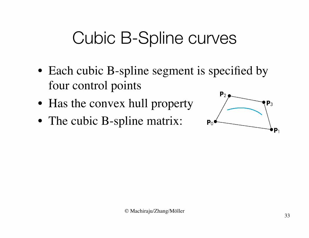
Cubic B-Spline curves• Each cubic B-spline segment is specified by
four control points• Has the convex hull property• The cubic B-spline matrix:
33
© Machiraju/Zhang/Möller
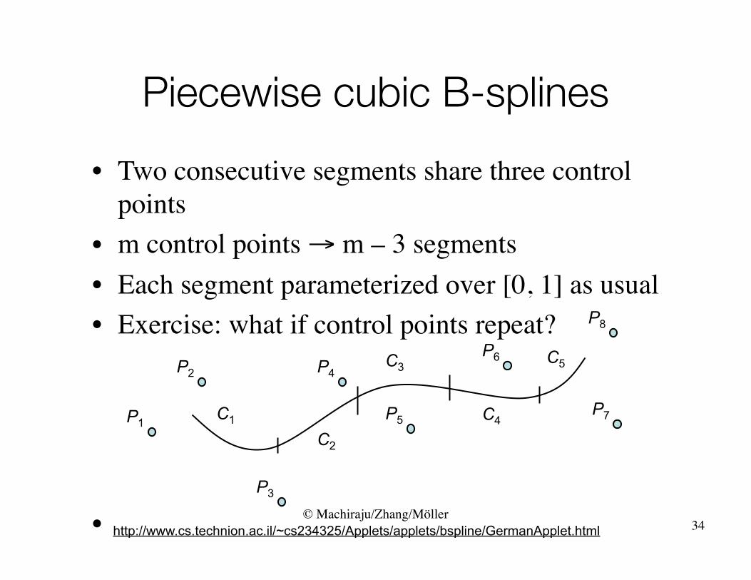
Piecewise cubic B-splines• Two consecutive segments share three control
points• m control points → m – 3 segments• Each segment parameterized over [0, 1] as usual• Exercise: what if control points repeat?
• http://www.cs.technion.ac.il/~cs234325/Applets/applets/bspline/GermanApplet.html 34
C1
C2
C3
C4
C5
P1
P3
P4
P5
P6
P8
P7
P2
© Machiraju/Zhang/Möller
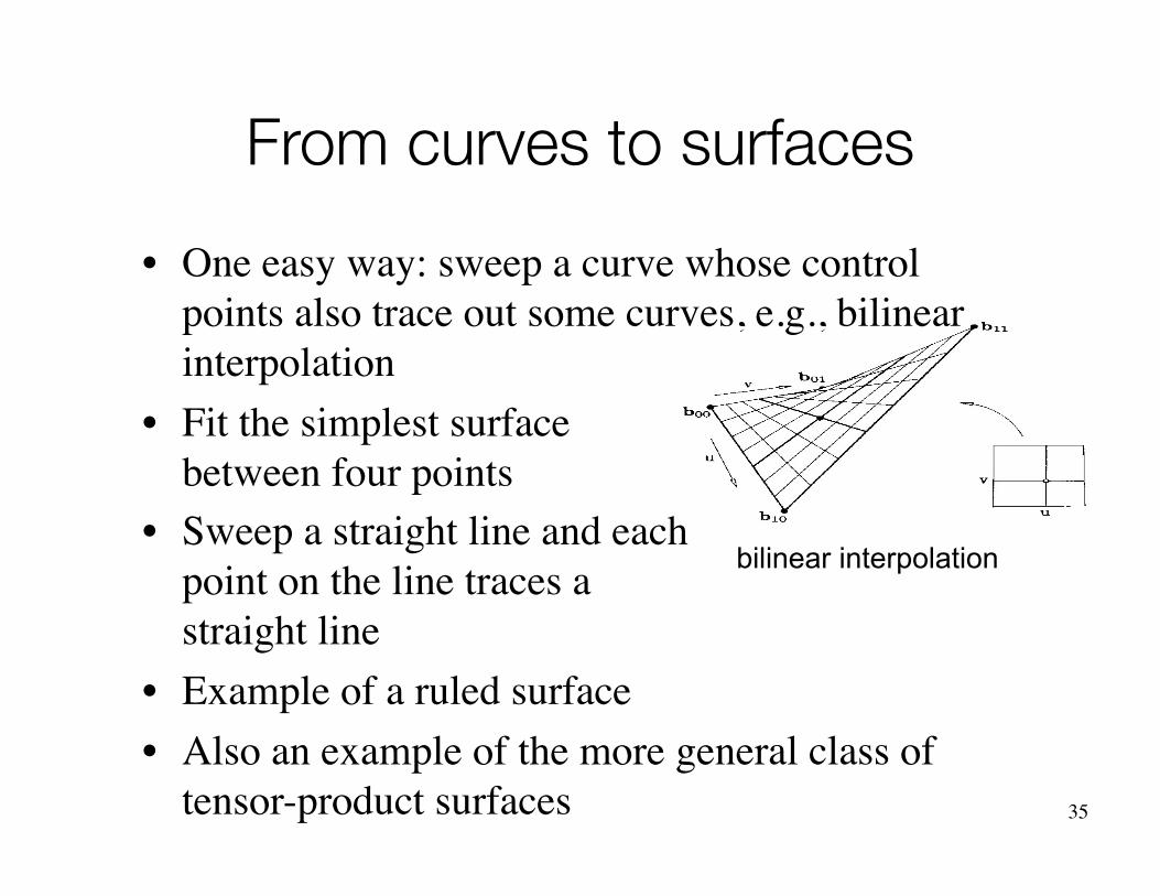
bilinear interpolation
From curves to surfaces• One easy way: sweep a curve whose control
points also trace out some curves, e.g., bilinear interpolation
• Fit the simplest surface between four points
• Sweep a straight line and each point on the line traces a straight line
• Example of a ruled surface• Also an example of the more general class of
tensor-product surfaces 35
© Machiraju/Zhang/Möller
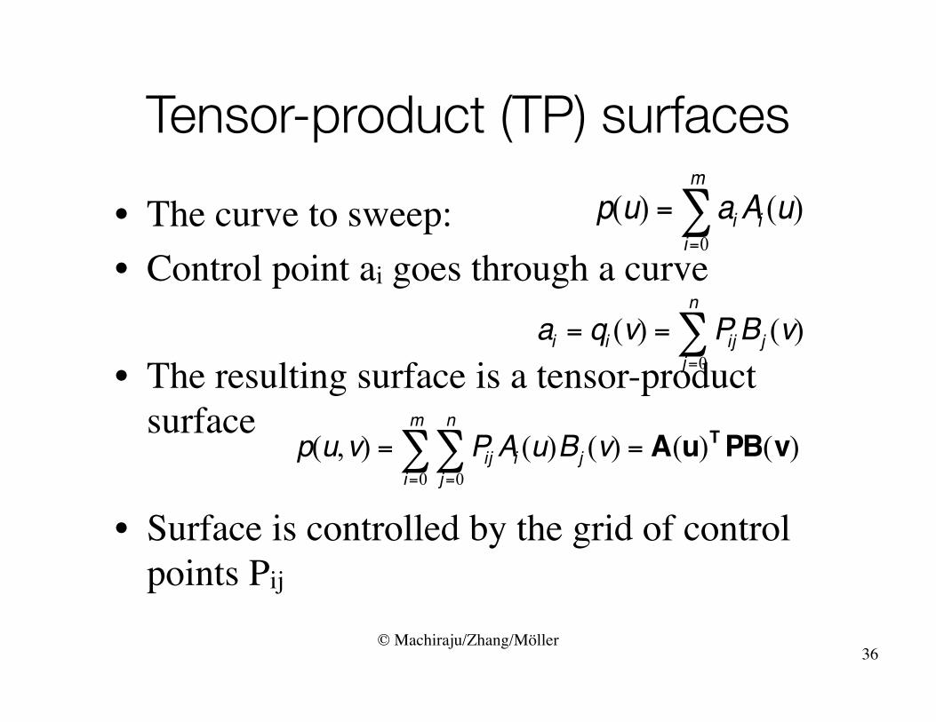
• The curve to sweep:• Control point ai goes through a curve
• The resulting surface is a tensor-product surface
• Surface is controlled by the grid of control points Pij
Tensor-product (TP) surfaces
36
© Machiraju/Zhang/Möller
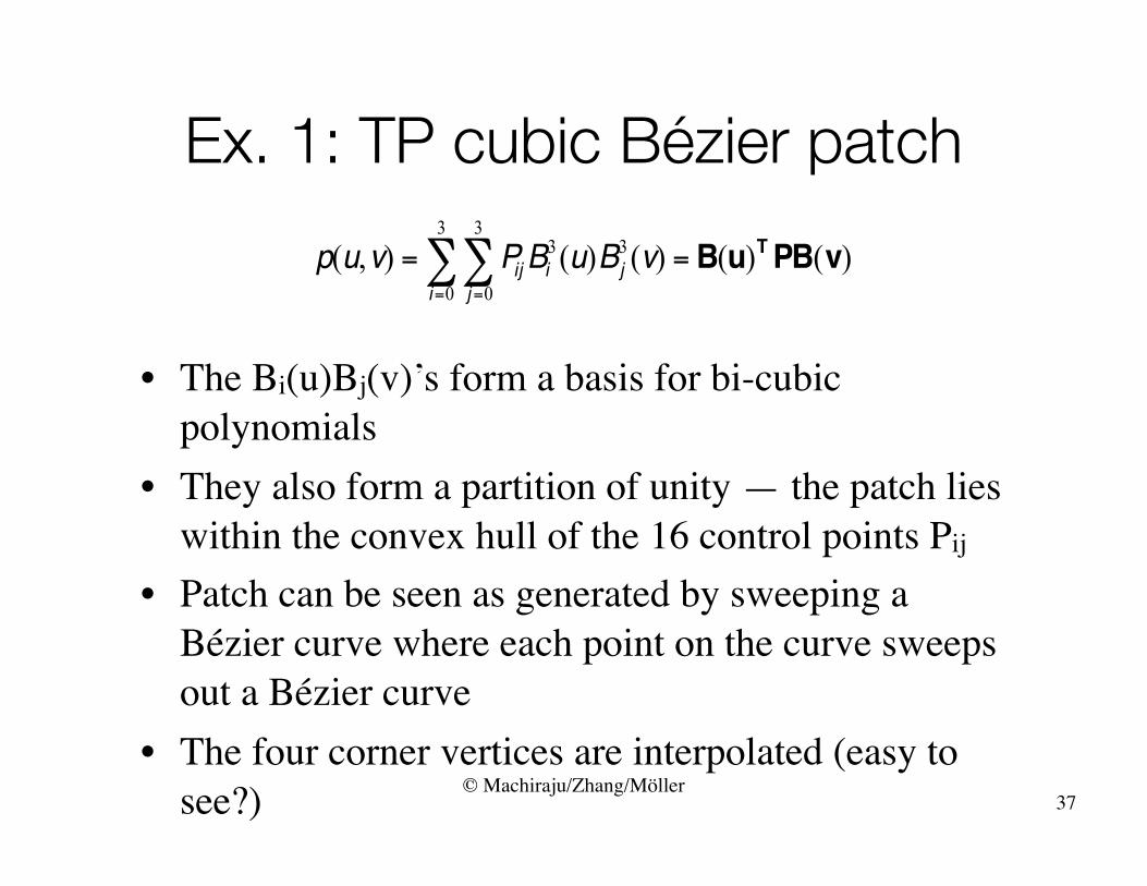
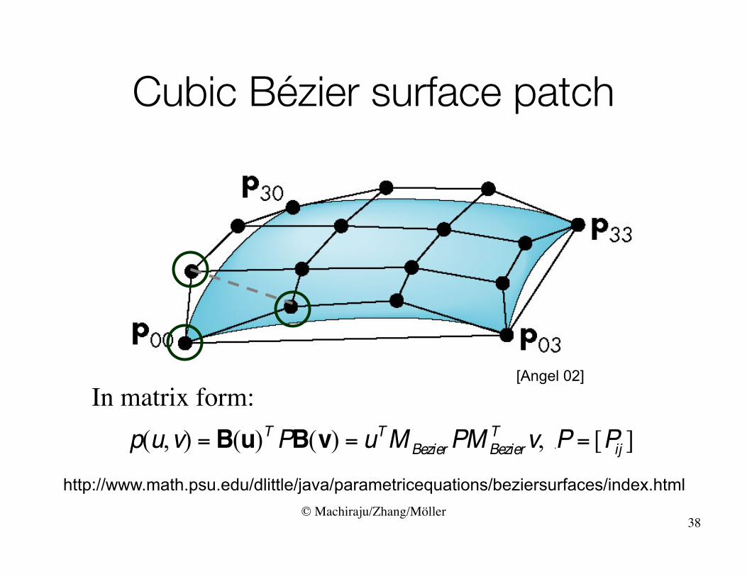
• The Bi(u)Bj(v)’s form a basis for bi-cubic polynomials
• They also form a partition of unity — the patch lies within the convex hull of the 16 control points Pij
• Patch can be seen as generated by sweeping a Bézier curve where each point on the curve sweeps out a Bézier curve
• The four corner vertices are interpolated (easy to see?)
Ex. 1: TP cubic Bézier patch
37
© Machiraju/Zhang/Möller
Cubic Bézier surface patch
38
In matrix form:[Angel 02]
http://www.math.psu.edu/dlittle/java/parametricequations/beziersurfaces/index.html
© Machiraju/Zhang/Möller
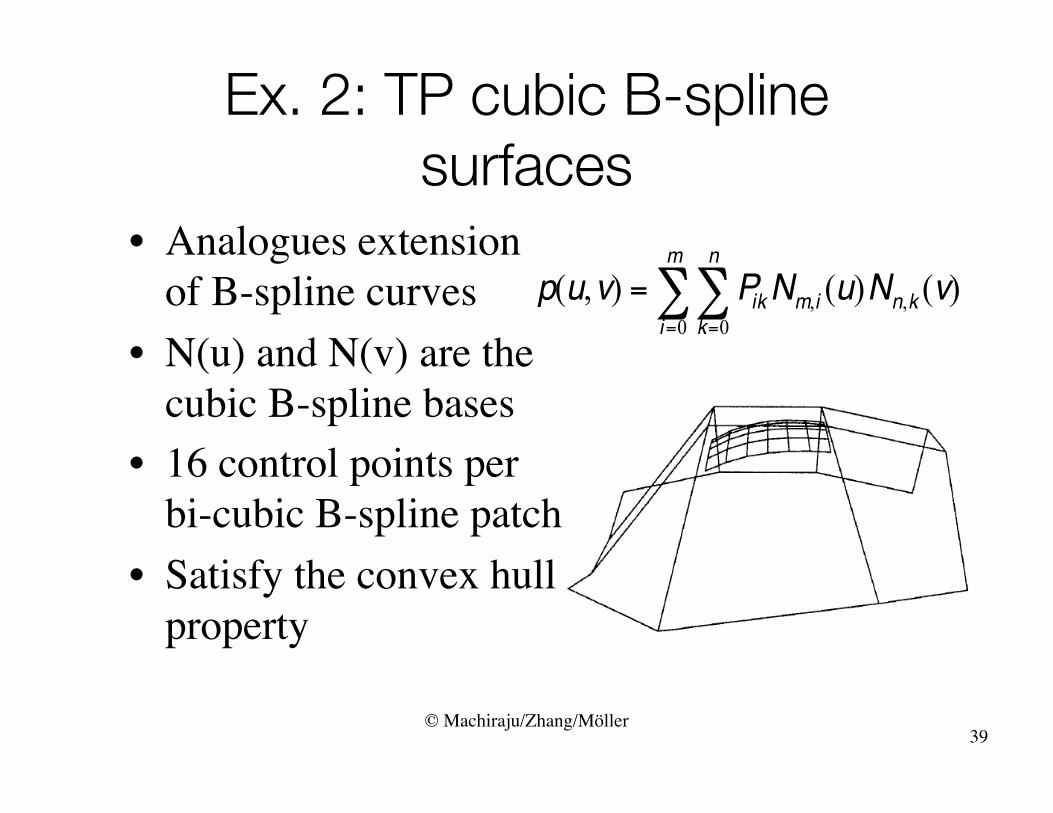
Ex. 2: TP cubic B-spline surfaces
• Analogues extension of B-spline curves
• N(u) and N(v) are the cubic B-spline bases
• 16 control points per bi-cubic B-spline patch
• Satisfy the convex hull property
39
© Machiraju/Zhang/Möller
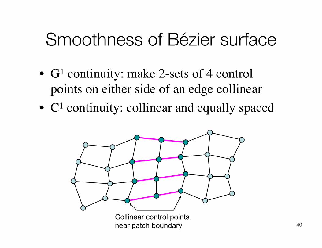
Smoothness of Bézier surface• G1 continuity: make 2-sets of 4 control
points on either side of an edge collinear• C1 continuity: collinear and equally spaced
40Collinear control points near patch boundary

© Machiraju/Zhang/Möller
Smoothness of B-spline surface
• C2 continuity is achieved if adjacent patches share control points
41
© Machiraju/Zhang/Möller
Today• Polynomials• Parametric representation• Fairness vs. smoothness• Parametric vs. geometric continuity• Hermite spline• Bezier spline• B-Spline• Surfaces• Subdivision 42
© Machiraju/Zhang/Möller
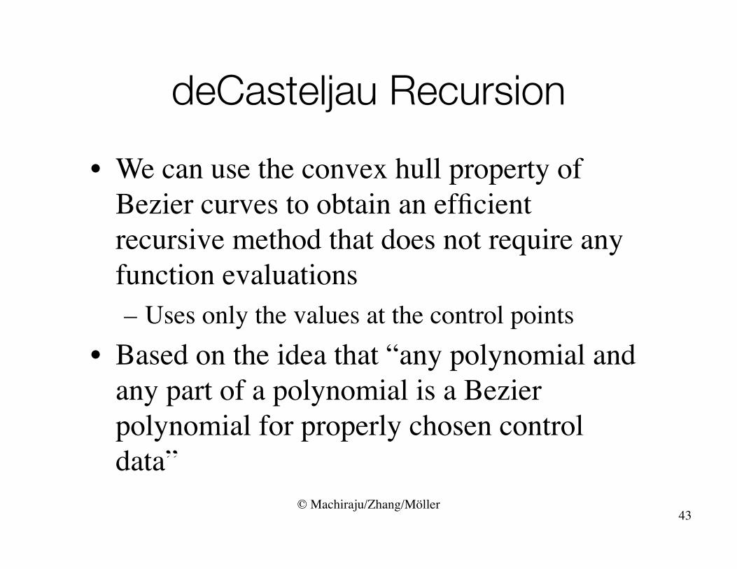
deCasteljau Recursion• We can use the convex hull property of
Bezier curves to obtain an efficient recursive method that does not require any function evaluations– Uses only the values at the control points
• Based on the idea that “any polynomial and any part of a polynomial is a Bezier polynomial for properly chosen control data”
43

• p0, p1, p2, p3 determine a cubic Bezier polynomial and its convex hull
© Machiraju/Zhang/Möller
Splitting a Cubic Bezier
Consider left half l(u) and right half r(u)44

© Machiraju/Zhang/Möller
l(u) and r(u)• Since l(u) and r(u) are Bezier curves, we
should be able to find two sets of control points {l0, l1, l2, l3} and {r0, r1, r2, r3} that determine them
45
© Machiraju/Zhang/Möller
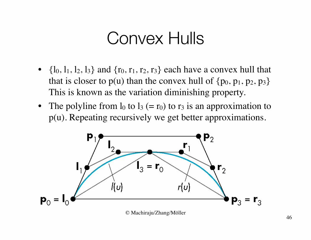
Convex Hulls• {l0, l1, l2, l3} and {r0, r1, r2, r3} each have a convex hull that
that is closer to p(u) than the convex hull of {p0, p1, p2, p3} This is known as the variation diminishing property.
• The polyline from l0 to l3 (= r0) to r3 is an approximation to p(u). Repeating recursively we get better approximations.
46

© Machiraju/Zhang/Möller
Equations• Start with Bezier equations p(u)=uTMBp• l(u) must interpolate p(0) and p(1/2)
• Matching slopes, taking into account that l(u) and r(u) only go over half the distance as p(u)
• Symmetric equations hold for r(u)47
l(0) = l0 = p0l(1) = l3 = p(1/2) = 1/8( p0 +3 p1 +3 p2 + p3 )
l’(0) = 3(l1 - l0) = p’(0) = 3/2(p1 - p0 )l’(1) = 3(l3 – l2) = p’(1/2) = 3/8(- p0 - p1+ p2 + p3)

© Machiraju/Zhang/Möller
Efficient Form
Requires only shifts and adds!
48
l0 = p0r3 = p3
l1 = ½(p0 + p1)r1 = ½(p2 + p3)
l2 = ½(l1 + ½( p1 + p2))r1 = ½(r2 + ½( p1 + p2))
l3 = r0 = ½(l2 + r1)
© Machiraju/Zhang/Möller
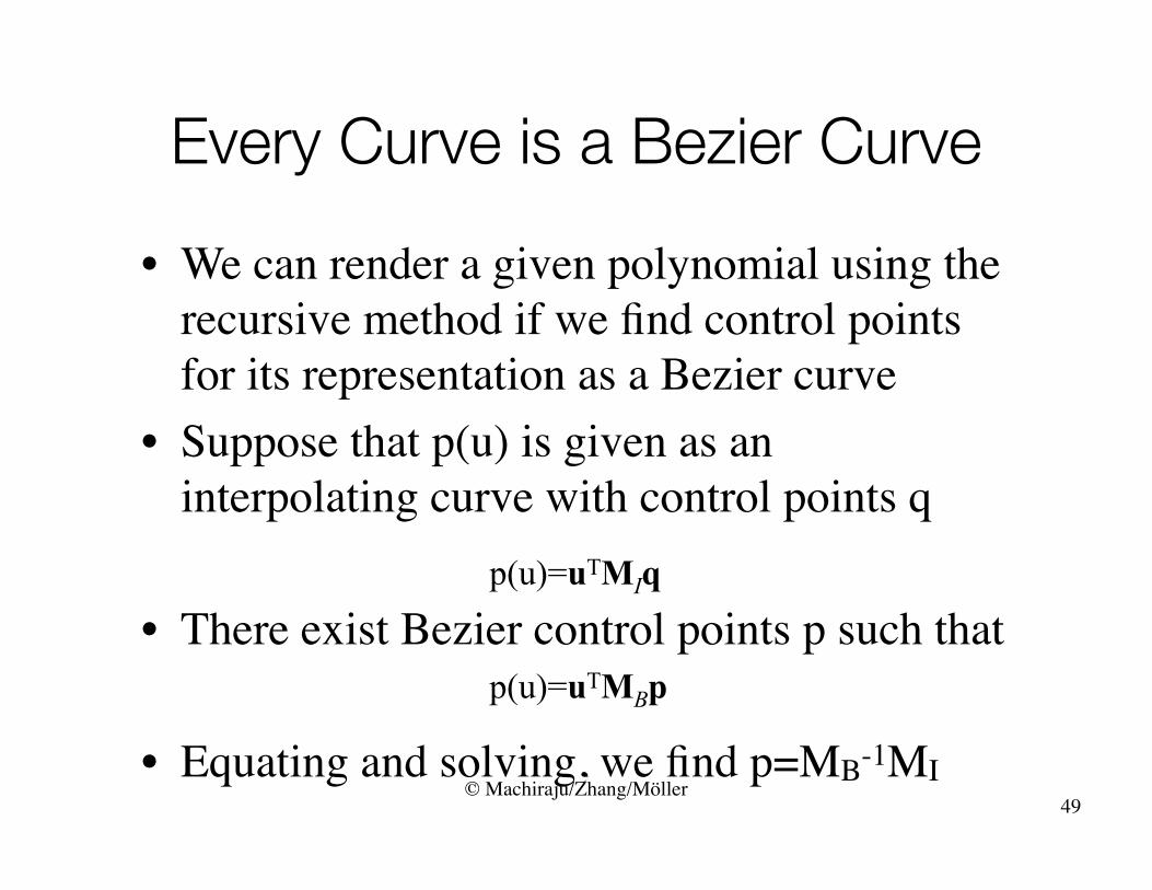
Every Curve is a Bezier Curve• We can render a given polynomial using the
recursive method if we find control points for its representation as a Bezier curve
• Suppose that p(u) is given as an interpolating curve with control points q
• There exist Bezier control points p such that
• Equating and solving, we find p=MB-1MI49
p(u)=uTMIq
p(u)=uTMBp
© Machiraju/Zhang/Möller
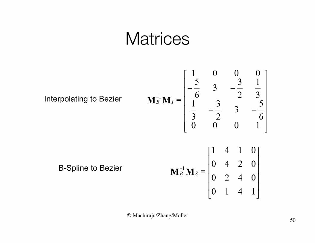
Matrices
Interpolating to Bezier
B-Spline to Bezier
50

© Machiraju/Zhang/Möller
Example
Bezier Interpolating B Spline
• These three curves were all generated from the same original data using Bezier recursion by converting all control point data to Bezier control points
51

© Machiraju/Zhang/Möller
Surfaces• Can apply the recursive method to surfaces if we
recall that for a Bezier patch curves of constant u (or v) are Bezier curves in u (or v)
• First subdivide in u – Process creates new points – Some of the original points are discarded
– 52original and kept new
original and discarded

© Machiraju/Zhang/Möller
Second Subdivision
53
16 final points for1 of 4 patches created

© Machiraju/Zhang/Möller
Normals• For rendering we need the normals if we
want to shade– Can compute from parametric equations
– Can use vertices of corner points to determine– OpenGL can compute automatically
54
© Machiraju/Zhang/Möller
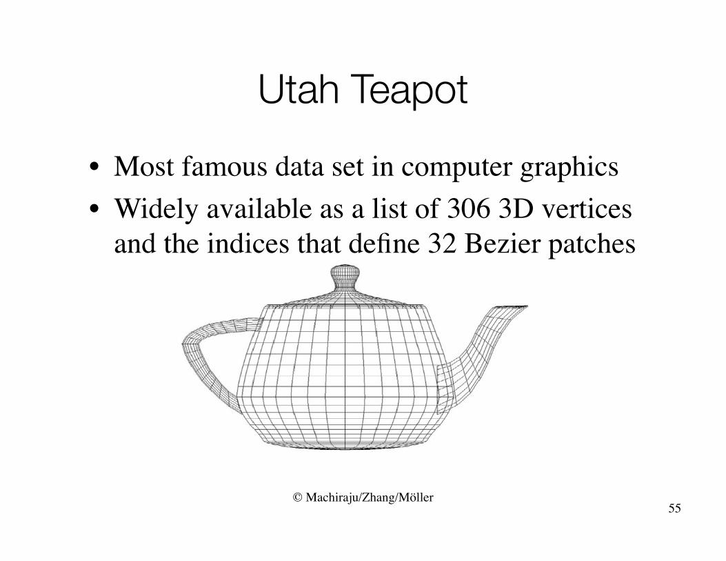
Utah Teapot• Most famous data set in computer graphics• Widely available as a list of 306 3D vertices
and the indices that define 32 Bezier patches
55
© Machiraju/Zhang/Möller
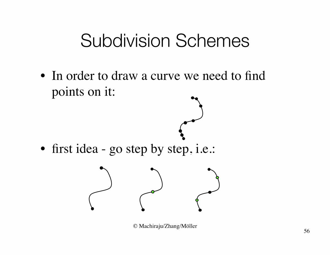
Subdivision Schemes• In order to draw a curve we need to find
points on it:
• first idea - go step by step, i.e.:
56
© Machiraju/Zhang/Möller
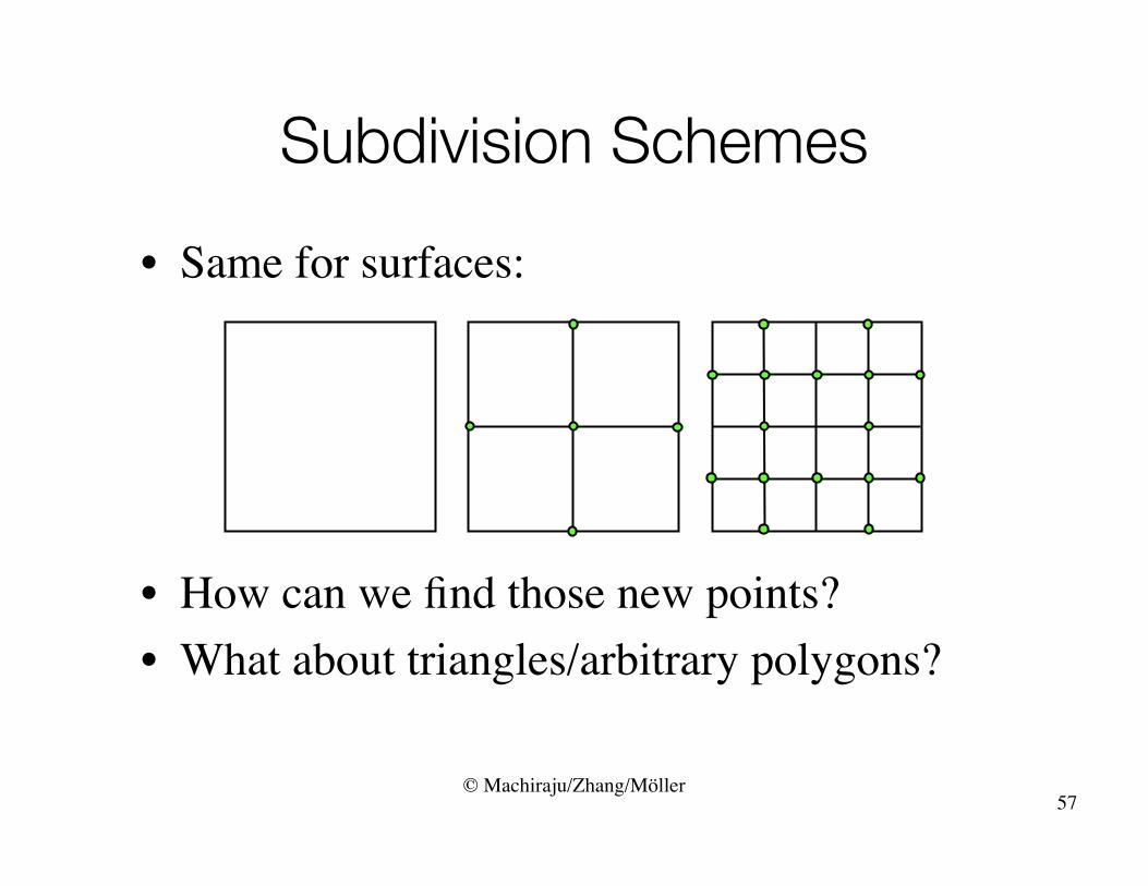
Subdivision Schemes• Same for surfaces:
• How can we find those new points?• What about triangles/arbitrary polygons?
57
© Machiraju/Zhang/Möller
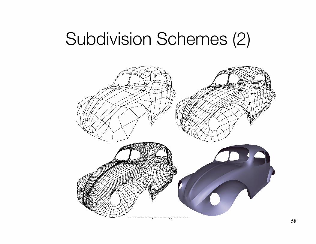
Subdivision Schemes (2)
58

© Machiraju/Zhang/Möller
Loop• Guaranteed to be smooth everywhere except
at extraordinary vertices• Face Split• Triangular
meshes• approximating
59

© Machiraju/Zhang/Möller
Loop (2)
60

© Machiraju/Zhang/Möller
Loop - Boundary• Subdivision Mask for
Boundary Conditions
61
Edge Rule Vertex Rule

© Machiraju/Zhang/Möller
Modified Butterfly• Face Split• Triangular
meshes• interpolating
62
© Machiraju/Zhang/Möller
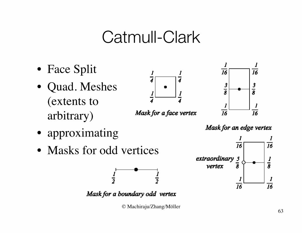
Catmull-Clark• Face Split• Quad. Meshes
(extents toarbitrary)
• approximating• Masks for odd vertices
63
© Machiraju/Zhang/Möller
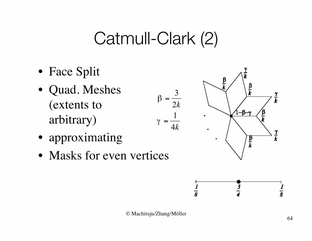
Catmull-Clark (2)• Face Split• Quad. Meshes
(extents toarbitrary)
• approximating• Masks for even vertices
64
© Machiraju/Zhang/Möller
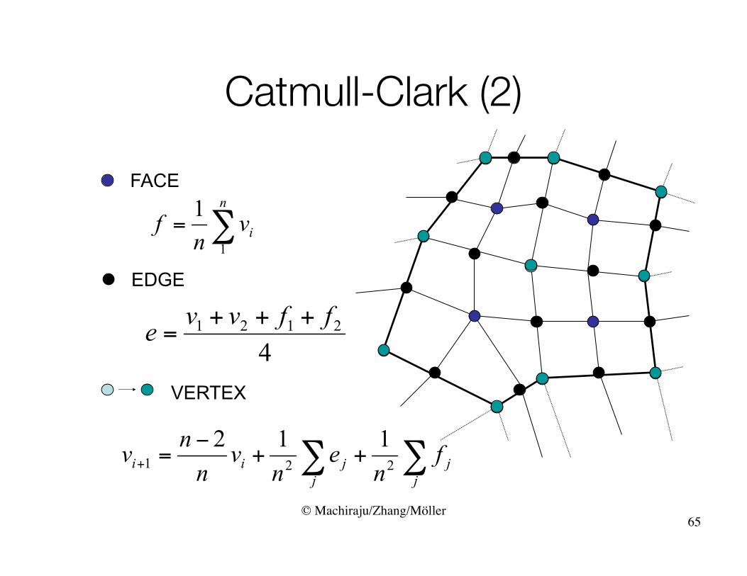
Catmull-Clark (2)
65
FACE
EDGE
VERTEX
© Machiraju/Zhang/Möller
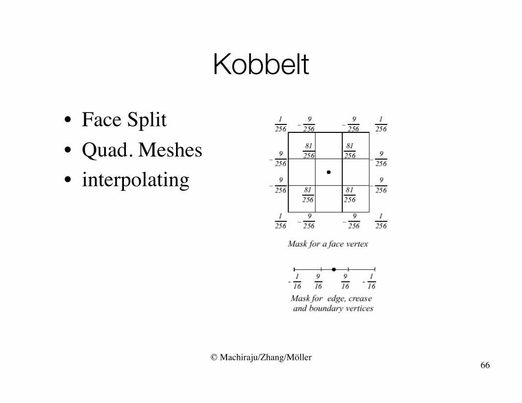
Kobbelt• Face Split• Quad. Meshes• interpolating
66
© Machiraju/Zhang/Möller
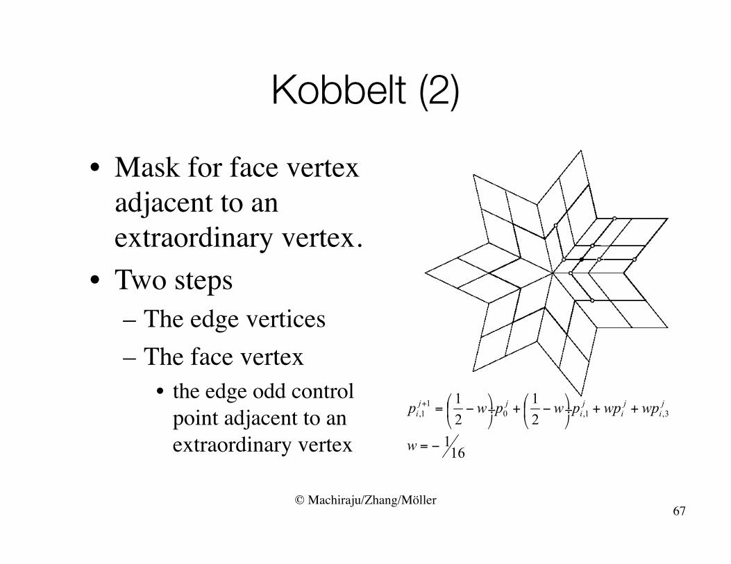
Kobbelt (2)• Mask for face vertex
adjacent to anextraordinary vertex.
• Two steps– The edge vertices– The face vertex
• the edge odd controlpoint adjacent to anextraordinary vertex
67
© Machiraju/Zhang/Möller
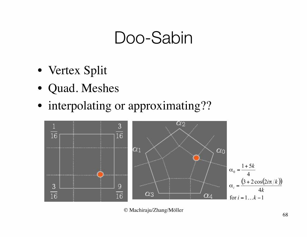
Doo-Sabin• Vertex Split• Quad. Meshes• interpolating or approximating??
68
© Machiraju/Zhang/Möller
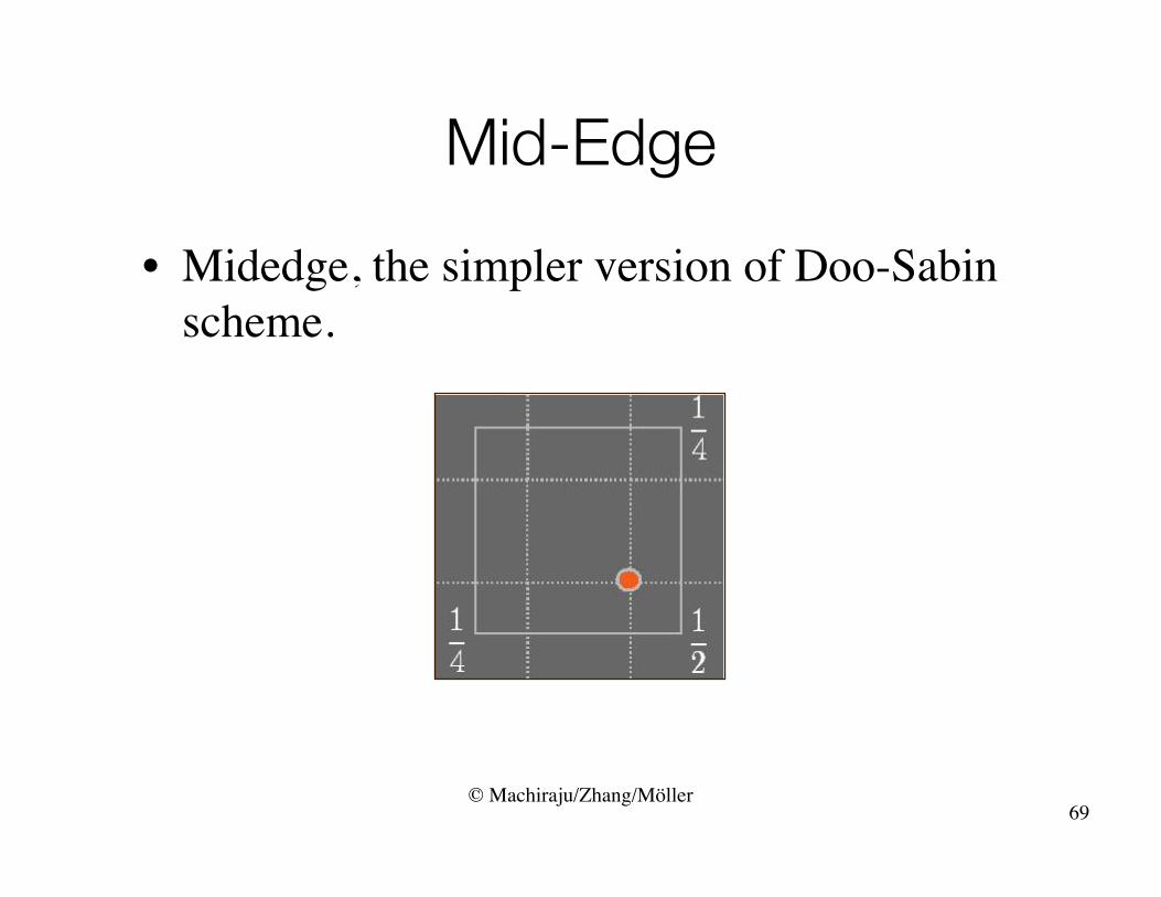
Mid-Edge• Midedge, the simpler version of Doo-Sabin
scheme.
69

© Machiraju/Zhang/Möller
Doo-Sabin & Mid-Edge• The interior rules can be decomposed into a
sequence of averaging steps.
Doo-Sabin scheme
Midedge scheme
70

© Machiraju/Zhang/Möller
Subdivision Schemes
Loop Butterfly
Catmull-Clark Doo-Sabin
71

© Machiraju/Zhang/Möller
Modeling with Subdivision• Subdivision produces smooth continuous
surfaces. • How can “sharpness” and creases be controlled
in a modeling environment? • ANSWER: Define new subdivision rules for
“creased” edges and vertices.– Tag Edges sharp edges.– If an edge is sharp, apply
new sharp subdivision rules.– Otherwise subdivide with
normal rules. 72