1

Subdivision curves and surfaces

Brian CurlessCSE 557

Fall 2014

2

Reading

Required:

Stollnitz, DeRose, and Salesin. Wavelets for Computer Graphics: Theory and Applications,1996, section 6.1-6.3, 10.2, A.5.

Note: there is an error in Stollnitz, et al., section A.5. Equation A.3 should read:

MV = V

This is already fixed in the handout.

3

Subdivision curves

Idea:

repeatedly refine the control polygon

curve is the limit of an infinite process

1 2 3P P P

lim jj

Q P

4

Chaikin’s algorithm

Chakin introduced the following “corner-cutting” scheme in 1974:

Start with a piecewise linear curve Insert new vertices at the midpoints (the

splitting step) Average each vertex with the “next” (clockwise)

neighbor (the averaging step) Go to the splitting step

5

Averaging masks

The limit curve is a quadratic B-spline!

Instead of averaging with the nearest neighbor, we can generalize by applying an averaging mask during the averaging step:

In the case of Chaikin’s algorithm:

r =

1 0 1r r r r

6

Lane-Riesenfeld algorithm (1980)

Use averaging masks from Pascal’s triangle:

Gives B-splines of degree n+1.

n=0:

n=1:

n=2:

1

0 12n

n n nr

n

7

Subdivide ad nauseum?

After each split-average step, we are closer to the limit curve.

How many steps until we reach the final (limit) position?

Can we push a vertex to its limit position in one step?

8

Local subdivision matrix

Consider the cubic B-spline subdivision mask:

Now consider what happens during splitting and averaging in a small neighborhood:

We can write equations that relate points at one subdivision level to points at the previous:

1 1 1

4 2 4

9

Local subdivision matrix

We can write this as a recurrence relation in matrix form:

where the L, R, C’s are (for convenience) row vectors.

In 2D, we can write out all the elements as follows:

We can re-write this as:

and M is the local subdivision matrix.

1

1

1

1/ 2 1/ 2 0

1/ 8 3 / 4 1/ 8

0 1/ 2 1/ 2

j j

j j

j j

L L

C C

R R

1 1

1 1

1 1

1 11/ 2 1/ 2 0

1 1/ 8 3 / 4 1/ 8 1

0 1/ 2 1/ 21 1

y yx xj j j j

y yx xj j j j

y yx xj j j j

L L L L

C C C C

R R R R

1j jA MA

10

Local subdivision matrix, cont’d

Starting from the initial control polygon, we can track the original vertex and its original neighborhood through subdivision:

The limit position of the neighborhood is then:

OK, so how do we apply a matrix an infinite number of times??

1j jA MA

0lim j

jA M A

11

Eigenvectors and eigenvalues

We now need to look at the eigenvectors and eigenvalues of M. Let v be a vector such that:

Mv = v

We say that v is an eigenvector of M with eigenvalue .

A 3x3 matrix can have 3 eigenvalues and eigenvectors:

In matrix form:

1 1 1

2 2 2

3 3 3

Mv v

Mv v

Mv v

1 2 3 1 1 2 2 3 3

1

1 2 3 2

3

0 0

0 0

0 0

M v v v v v v

v v v

MV = V

12

To infinity, but not beyond…

Now let’s apply M to original neigborhood A0:

Now let’s advance another subdivision:

Do it j times:

What if we do this an infinite number of times?

Let’s assume the eigenvalues are non-negative and sorted so that:

If 1 > 1, then:

If 1 < 1, then:

If 1 = 1, then:

1 2 3 0n

1 0A MA

212 0A M A MA

0A M A

0j

jA M A

13

Evaluation masks

For cubic B-splines, the local subdivision matrix M is:

It’s eigenvalues and eigenvectors are:

1 = 1 > 2 > 3, so we’re OK!

We can write out and V:

We will also need V-1, which turns out to be:

1

1

1

1

1

1

v

2

2

1

21

0

1

v

3

3

1

42

1

2

v

1 0 0 1 1 2

0 1/ 2 0 1 0 1

0 0 1/ 4 1 1 2

V

1

1/ 6 2 / 3 1/ 6

1/ 2 0 1/ 2

1/ 6 1/ 3 1/ 6

V

1/ 2 1/ 2 0

1/ 8 3 / 4 1/ 8

0 1/ 2 1/ 2

M

14

Evaluation masks (cont’d)

So, we have:

We can now compute the limit position of the neighborhood A0 :

1

1 0 0 1 1 2 1/ 6 2 / 3 1/ 6

0 1/ 2 0 1 0 1 1/ 2 0 1/ 2

0 0 1/ 4 1 1 2 1/ 6 1/ 3 1/ 6

V V

1

0 0A M A V V A

15

The row vector that pushes the original vertex to the limit position is called the evaluation mask:

Note that we do not need start with the 0th level control points and push them to the limit.

If we subdivide and average the control polygon jtimes, we can push the vertices of the refined polygon to the limit as well:

Now we can cook up a simple procedure for creating subdivision curves:

Subdivide (split+average) the control polygon a few times. Use the averaging mask.

Push the resulting points to the limit positions. Use the evaluation mask.

Recipe for subdivision curves

1

Tj jA M A u A

1

1 2 1

6 3 6Tu

1Tu

16

Tangent analysis

1

1

1

yxj j

yxj j j

yxj j

L L

A C C

R R

17

Tangent analysis (cont’d)

1 1 1 2 2 2 3 3 3 0j T j T j T

j w w w At u u u 1 2 3 0n

18

DLG interpolating scheme (1987)

Slight modification to subdivision algorithm:

splitting step introduces midpoints averaging step only changes midpoints

For DLG (Dyn-Levin-Gregory), use:

Since we are only changing the midpoints, the points after the averaging step do not move.

newold1

(1) ( 2,5,10,5, 2)16

r r

19

Building complex models

We can extend the idea of subdivision from curves to surfaces…

20

Subdivision surfaces

Chaikin’s use of subdivision for curves inspired similar techniques for subdivision surfaces.

Iteratively refine a control polyhedron (or control mesh) to produce the limit surface

using splitting and averaging steps.

lim j

jS P

0P 1P 2P P

21

Triangular subdivision

There are a variety of ways to subdivide a poylgonmesh.

A common choice for triangle meshes is 4:1 subdivision – each triangular face is split into four smaller triangles:

22

Loop averaging step

Once again we can use masks for the averaging step:

where

These values, due to Charles Loop, are carefully chosen to ensure smoothness – namely, tangent plane or normal continuity.

Note: tangent plane continuity is also know as G1

continuity for surfaces.

32

))/2cos(23(

4

5)(

)(

))(1()(

2nn

n

nnn

1( )

( )nn

n n

Q Q QQ

23

Loop evaluation and tangent masks

As with subdivision curves, we can split and average a number of times and then push the points to their limit positions.

where

How do we compute the normal?

cosi3n

(n) = (n) = (2 i/n)(n)

1

1 1 1 2 2

1 1 12 2

( )

( )

( ) ( ) ( )

( ) ( ) ( )

n

n n

n nn

n

n n

n n n

n n n

Q Q QQ

T Q Q Q

T Q Q Q

24

Recipe for subdivision surfaces

As with subdivision curves, we can now describe a recipe for creating and rendering subdivision surfaces:

Subdivide (split+average) the control polyhedron a few times. Use the averaging mask.

Compute two tangent vectors using the tangent masks.

Compute the normal from the tangent vectors. Push the resulting points to the limit positions.

Use the evaluation mask. Render!

25

Adding creases without trim curves

For NURBS surfaces, adding sharp features like creases required the use of trim curves.

For subdivision surfaces, we can just modify the subdivision masks. E.g., we can mark some edges and vertices as “creases” and modify the subdivision mask for them (and their children):

This gives rise to G0 continuous surfaces (i.e., having positional but not tangent plane continuity).

[Hop

pe, S

IGG

RAPH

199

4]

26

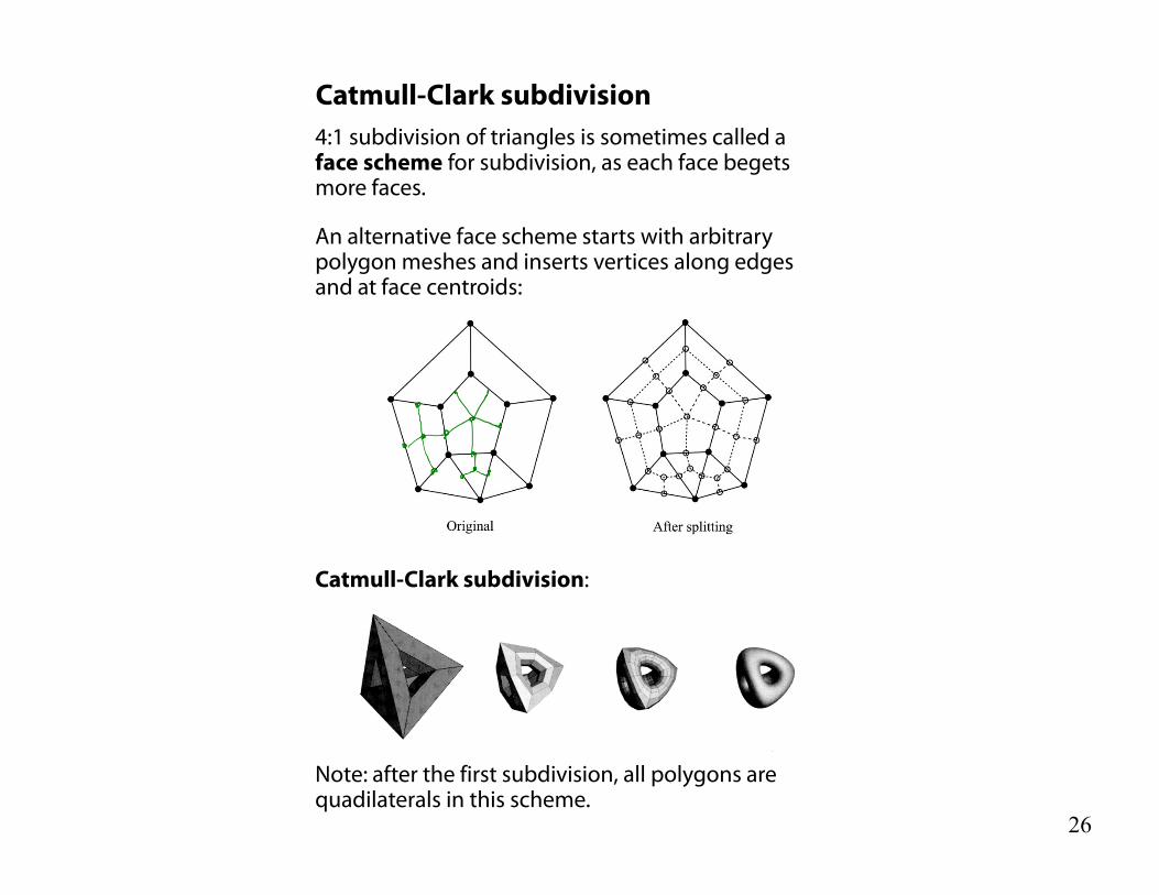
Catmull-Clark subdivision4:1 subdivision of triangles is sometimes called a face scheme for subdivision, as each face begets more faces.

An alternative face scheme starts with arbitrary polygon meshes and inserts vertices along edges and at face centroids:

Catmull-Clark subdivision:

Note: after the first subdivision, all polygons are quadilaterals in this scheme.

27

Creases without trim curves, cont.

Here’s an example using Catmull-Clark surfaces (based on subdividing quadrilateral meshes):

This particular example uses the hybrid technique of DeRose, et al., which applies sharp subdivision rules at some creases for a finite number of steps, and then switches to smooth subdivision, giving more gentle creases. This technique was used in Geri’s Game.

28

Interpolating subdivision surfaces

Interpolating schemes are defined by

splitting averaging only new vertices

The following averaging mask is used in butterfly subdivision:

Setting t=0 gives the original polyhedron, and increasing small values of t makes the surface smoother, until t=1/8 when the surface is provably G1.