3.2dapertures

7/26/2019 3.2DApertures

http://slidepdf.com/reader/full/32dapertures 1/10

Two-Dimensional Aperture Antennas

The field pattern of a two-dimensional aperture

The method we used to show that the field pattern of a one-dimensional aperture is the

one-dimensional Fourier transform of the aperture field illumination can simply be generalized to the

more realistic case of a two-dimensional aperture:

where m is the y -axis analog of l on the x-axis, and . In words,

The electric field pattern of a two-dimensional aperture is the two-dimensional Fourier transform

of the aperture field illumination.

The Uniformly Illuminated Rectangular Aperture

A two-dimensional rectangular aperture with side lengths D and D . Dividing lengths in the

aperture plane by the wavelength Õ yield the normalized coordinates and . The

direction from the origin to any distant point can be specified by and , where Ò

is the angle from the (y; ) plane and Ò is the angle from the (x; ) plane.

The two-dimensional counterpart of a uniformly illuminated one-dimensional aperture is a uniformly

illuminated rectangular aperture with sides D and D . If the illumination g (x; ) is constant over the

aperture, the integrals over u and v in the Fourier transform are separable and

f (l; ) (u; )e dudv m /Z 1

À1

Z 1À1

g v Ài2Ù (lu+mv) (3C1)

v =Õ Ñ y

x y

u =Õ Ñ x v =Õ Ñ y

l Ñ sin Ò x m Ñ sin Ò y x

z y z

x y y

f (l; ) sinc ; m / sinc

Ò Õ

lDxÓ Ò

Õ

mDyÓ

wo-Dimensional Aperture Antennas http://www.cv.nrao.edu/course/astr534/2DApertu

of 10 09/27/2010 12:1



where

Squaring the electric field pattern gives the relative (normalized to unity at the peak) power pattern

Given the relative power pattern, we can calculate the absolute power gain G in any direction by

invoking energy conservation:

Defining the temporary variable a:

gives, for ,

since we can look up the definite integral in square brackets; its value is Ù .

4Ù :

Thus the peak power gain is

G

and the power pattern of a uniformly illuminated rectangular aperture with side lengths D and D is

when Ò and Ò are much smaller than one radian.

In general, the peak power gain of an aperture antenna is proportional to the geometric area A(A D in this case) of the aperture. The constant of proportionality is 4Ù=Õ for a

uniformly illuminated aperture and somewhat less for any other illumination pattern.

sinc(x) (Ùx)=(Ùx) : Ñ sin

P (l; ) sinc n m = sinc2

Ò Õ

lDx

Ó 2

Ò Õ

mDy

Ó

d Ê Ù (l; )dl m

Z G = 4 = G0

Z À1

+1 Z À1

+1

P n m d

4Ù dl dm = G0

Z À1

+1"

ÙlD =Õx

sin(ÙlD =Õ)x

#2 Z À1

+1"

ÙmD =Õy

sin(ÙmD =Õ)y

#2

a ; so da dl Ñ Õ

ÙlDx =

Õ

ÙDx

D x µ Õ

dl da

Z À1

+1"

ÙlD =Õx

sin(ÙlD =Õ)x

#2

ÙÔZ 1

À1 a2

sin2 a Õ

Õ

ÙDx=

Õ

Dx

= G0

Õ2

D Dx y

0 =Õ2

4ÙD Dx y

x y

G sinc sinc sinc sinc =Õ2

4ÙD Dx y 2

Ò Õ

lDxÓ

2

Ò Õ

mDyÓ

Ù Õ2

4ÙD Dx y 2

Ò Õ

Ò Dx xÓ

2

Ò Õ

Ò Dy yÓ

(3C

x y

geom

geom = Dx y 2


of 10 09/27/2010 12:1



Using the relation

A

we find that the on-axis effective collecting area is

max(A ) D

The peak effective area of an ideal uniformly illuminated aperture equals its geometric area,

independent of wavelength. With any other illumination taper, the effective area is smaller than but

proportional to the geometric area. It is useful to define the aperture efficiency Ñ as the ratio of

the effective area to geometric area:

Ñ

Thus Ñ for an ideal uniformly illuminated aperture and Ñ otherwise.

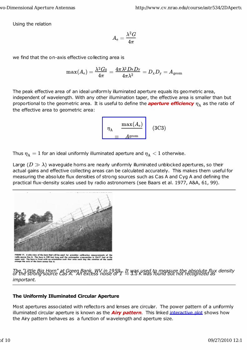
Large ( ) waveguide horns are nearly uniformly illuminated unblocked apertures, so their

actual gains and effective collecting areas can be calculated accurately. This makes them useful for

measuring the absolute flux densities of strong sources such as Cas A and Cyg A and defining the

practical flux-density scales used by radio astronomers (see Baars et al. 1977, A&A, 61, 99).

The "Little Big Horn" at Green Bank, WV in 1959. It was used to measure the absolute flux density of the strong source Cas A. An excess noise of K was found but not recognized as

important.

The Uniformly Illuminated Circular Aperture

Most apertures associated with reflectors and lenses are circular. The power pattern of a uniformly

illuminated circular aperture is known as the Airy pattern. This linked interactive plot shows how

the Airy pattern behaves as a function of wavelength and aperture size.

e =4Ù

Õ G2

e =4Ù

Õ G2 0 =4ÙÕ2

4ÙÕ D D2 x y= Dx y = Ageom

A

A

Ñ Ageom

max(A )e(3C3)

A = 1 A < 1

D µ Õ

T :5 Ù 3


of 10 09/27/2010 12:1



The Circular Gaussian Illumination Pattern

A good approximation for "real" radio telescopes with practical feeds and circular apertures is a

circular Gaussian illumination pattern. The normalized Gaussian function g (u) in one dimension is

defined by

where Û is the rms (root mean square) width defined by

and "normalized" means .

This bell-shaped curve is a plot of the (not normalized) Gaussian function .

For the circular Gaussian illumination pattern

the field pattern is

where Û is the rms radius of the illumination pattern in wavelengths. The function f (l; ) isseparable:

where

g (u)

À ;

Ñ

1

Û p 2Ù

expÒ u2

2Û 2Ó

Û g (u)du (u)du ÑÔZ 1

À1u2

¶Z 1À1

g

Õ1=2

(u)du R 1

À1 g = 1

g [Àu =(2Û )] = exp 2 2

exp À À À

Ò 2Û 2u2 + v2Ó

= exp

Ò u2

2Û 2

Óexp

Ò v2

2Û 2

Ó

f (l; ) À À [Ài2Ù (lu v)]dudv ; m /Z 1

À1

Z 1À1

exp

Ò u2

2Û 2

Óexp

Ò v2

2Û 2

Óexp + m

m

f (l; ) (l) (m); m / f Â f


of 10 09/27/2010 12:1



and

Each integral is the one-dimensional Fourier transform of a Gaussian. The Fourier transform of the

Gaussian is the Gaussian (derivation). Given this Fourier

transform of the Gaussian with 2ÙÛ , we can use the similarity theorem with to

get

so the field pattern of an aperture with circular Gaussian illumination is

and the normalized power pattern is

For a reflector many wavelengths across, so and . Thus the power pattern

produced by circular Gaussian illumination is also a circular Gaussian.

The half-power beamwidth Ò is the solution of

(2)

where Û is the rms width of the illumination pattern in wavelengths.

Since a Gaussian extends to , this calculation formally assumes that the aperture itself is infinite.However, the Gaussian illumination g (u; ) falls off exponentially and is negligible for .

In practice, the value of Û is chosen so that g (u; ) is down quite a bit (e.g., 15 or 20 dB) at the

edge of the actual finite reflector. Tapering (or grading) the illumination this way:

(1) broadens the beamwidth Ò slightly,

(2) reduces the aperture efficiency Ñ slightly,

(3) reduces the sidelobe level significantly, and

(4) reduces spillover (wasted power, increased noise from ground pickup) significantly

compared with uniform illumination.

f (l) À (Ài2Ùlu)du ÑZ 1

À1exp

Ò u2

2Û 2

Óexp

f (m) À (Ài2Ùmv)dv ÑZ

1

À1

exp

Ò v2

2Û 2

Óexp

f (x) (ÀÙx ) = exp 2 F (s) (ÀÙs ) = exp 2

2 = 1 a Û ) = (p

2Ù À1

f (l) (ÀÙl ÙÛ ) / exp 2 Â 2 2

f (m) (ÀÙm ÙÛ ) / exp 2 Â 2 2

f (l; ) [À2Ù Û (l )] m / exp 2 2 2 + m2

P (l; ) f (l; )] [À4Ù Û (l )] : n m = [ m 2 / exp 2 2 2 + m2

Û µ 1 l Ù Ò x m Ù Ò y

HPBW

exp À4Ù Û

Ô 2 2

Ò 2

Ò HPBWÓ

2Õ

=2

1

4

4Ù Û Ò 2 2 2HPBW = ln

Ò radians; HPBW =ÙÛ

p ln(2)

Æ1 v u 2 + v2 µ Û 2

v

HPBW

A


of 10 09/27/2010 12:1



Spillover is illumination extending beyond the aperture. Here the relative field strength at the edge

is Î .

Using Gaussian tapering as an example, let

Î

be the tapered field strength at the edge of the reflector. Thus Î :1 (field taper) corresponds to

Î :01 (power taper), or a 20 dB edge taper. This corresponds to an aperture of radius

. For small Î our previous calculation, which assumed an infinite aperture so Î , will

slightly underestimate the beamwidth of a finite reflector but still be fairly accurate because only a

small fraction of the illumination will "spill over" the edge of the reflector. For a circular reflector with

diameter D,

u

and

Then

Recall that the beamwidth for Î is

so for a finite aperture,

Ñ g (0; )0g (u ; )ma x 0

= 02 = 0

Ù :15Û 2 = 0

ma x = D

2Õ

Î À : =g (0; )0

g (u ; )ma x 0= exp

Ò 2Û 2

u2ma x

Ó

À (Î ) : ln =2Û 2

u2ma x =

D2

8Õ Û 2 2

= 0

Ò ; HPBW =ÙÛ

p ln(2)

Ò Õ HPBW Ù ÙD

p ln(2)q

À8 (Î )ln


of 10 09/27/2010 12:1



Example: What is the half-power beamwidth of a circular aperture with a Gaussian illumination

tapering to Î :1 at the edge?

Example: Estimate the beamwidth in arcsec of the GBT (D 00 m) as a function of frequency in

GHz.

Ò

This estimate is slightly low, as expected. The measured beamwidth of the GBT is about 740 arcsec

/ · (GHz), or about 1:2Õ=D.

A good approximation for the half-power beamwidths of most single-dish radio telescopes is

Ò :2Õ=D

Reflector Accuracy Requirements

Real radio telescopes don't have perfectly paraboloidal reflectors. Small deviations from the best-fit

paraboloid may be caused by permanent manufacturing errors, changing gravitational deformations

as the reflector is tilted, thermal distortions resulting from solar heating, and bending by strong

winds. There will be some shortest wavelength Õ below which these errors degrade the reflector

performance so severely that the telescope becomes unusable. We can define the reflector

surface efficiency Ñ as the power gain of the actual reflector divided by the power gain of a

perfectly paraboloidal reflector with the same size and illumination. Next we will calculate how Ñ

Ò HPBW Ù Ù

p À8 (2) (Î )ln ln Õ

D

= 0

Ò :14 HPBW Ù Ù

p À8 (2) (0:1)ln ln Õ

D Ù 1

Õ

D

= 1

Ò :14 HPBW Ù 1 c

·D

Ò :14 rad 06265 arcsec=rad HPBW Ù 1 Â 2 ÂÒ

3:00 0 m sÂ 1 8 À1

· (GHz) 0 Hz=GHz 00 mÂ 1 9 Â 1

Ó

HPBW Ù · (GHz)

705 arcsec

HPBW Ù 1 (3C4)

min

s

s


of 10 09/27/2010 12:1



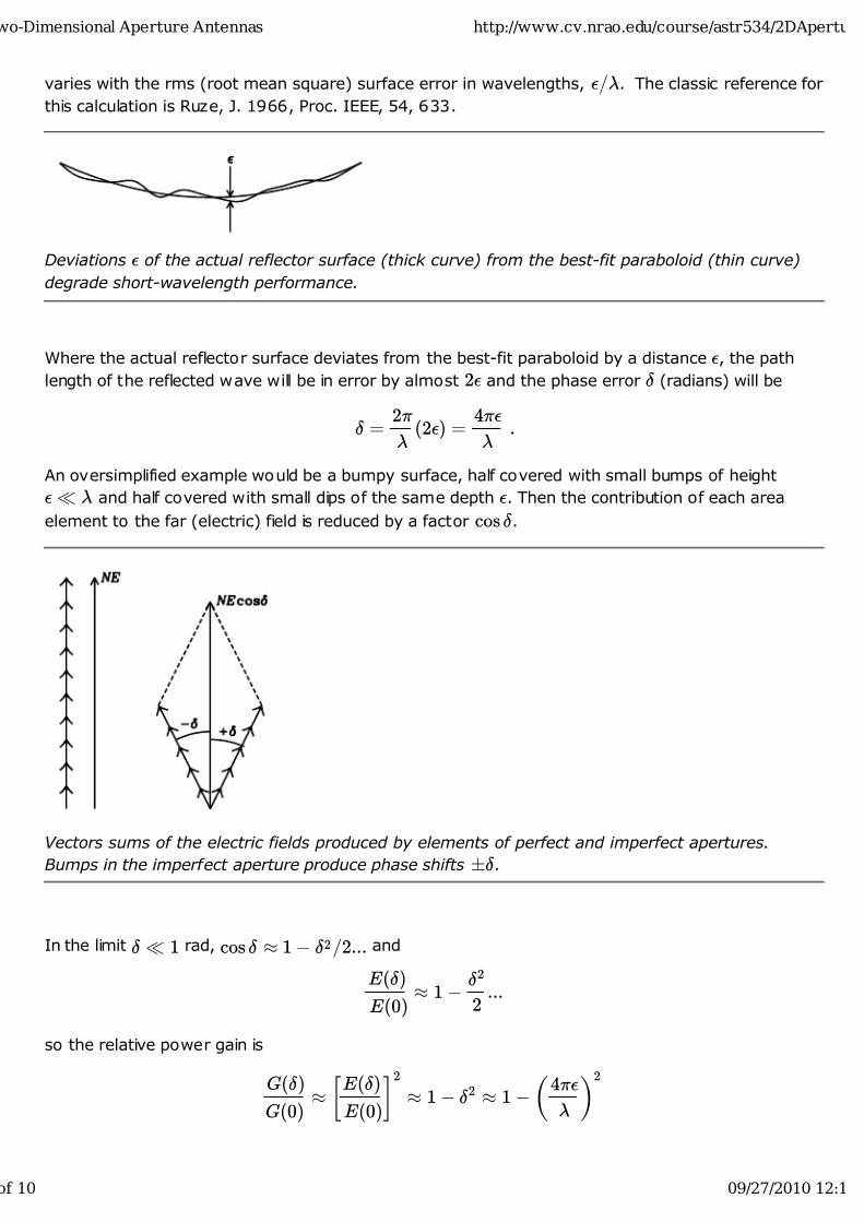
varies with the rms (root mean square) surface error in wavelengths, Ï=Õ. The classic reference for

this calculation is Ruze, J. 1966, Proc. IEEE, 54, 633.

Deviations Ï of the actual reflector surface (thick curve) from the best-fit paraboloid (thin curve)

degrade short-wavelength performance.

Where the actual reflector surface deviates from the best-fit paraboloid by a distance Ï, the path

length of the reflected wave will be in error by almost 2Ï and the phase error Î (radians) will be

Î (2Ï) :

An oversimplified example would be a bumpy surface, half covered with small bumps of height

and half covered with small dips of the same depth Ï. Then the contribution of each area

element to the far (electric) field is reduced by a factor cos .

Vectors sums of the electric fields produced by elements of perfect and imperfect apertures.

Bumps in the imperfect aperture produce phase shifts .

In the limit rad, and

:::

so the relative power gain is

=Õ

2Ù =

Õ

4ÙÏ

Ï Ü ÕÎ

ÆÎ

Î Ü 1 cos =2::: Î Ù 1 À Î 2

E (0)

E (Î ) Ù 1 À 2

Î 2

G(Î )

G(0)ÙÔ

E (0)

E (Î )Õ2

Ù 1 À Î 2 Ù 1 ÀÒ

Õ

4ÙÏÓ2


of 10 09/27/2010 12:1



This rough estimate shows that the surface errors must be an order-of-magnitude smaller than the

shortest usable wavelength, a severe requirement indeed.

A more realistic calculation makes use of the fact the most error distributions are roughly Gaussian.

Suppose that the surface errors have a Gaussian probability distribution P with rms Û :

where the normalization factor in front of the exponential term ensures that

as required for any probability distribution. Then the relative field strength is obtained as the

weighted sum over all possible Ï:

By substituting e (z ) (z ) we can turn this integral into a more familiar one, the Fourier

transform of a Gaussian:

Note that the i (z ) part drops out immediately because it is antisymmetric over the symmetric

region of integration. To make this look even more like our usual form for a Fourier transform, let

, , and . Then

Recall that

and apply the similarity theorem to get

h i [À2Ù Û s ]

Power is proportional to E so our final result for the reflector surface efficiency is

P (Ï)

À ; =

1

Û p 2Ù

expÒ Ï2

2Û 2Ó

(Ï)dÏ

Z 1À1

P = 1

h i À dÏ E

E (0)Ù Z

1

À1

cosÒ Õ

4ÙÏ

ÓÂ 1

Û p

2Ù expÒ

Ï2

2Û 2Óiz = cos + i sin

h i Ài À dÏ : E

E (0)ÙZ 1

À1exp

Ò Õ

4ÙÏÓ

Â 1

Û p

2Ù exp

Ò ÙÏ2

2ÙÛ 2

Ó

sin

s =Õ Ñ 2 x Ñ Ï a Û ) Ñ (p

2Ù À1

h i (Ài2Ùsx) [ÀÙ (ax) ]dx : E E (0)

ÙZ 1

À1exp exp 2

f (x) (ÀÙx ) has Fourier transform F (S ) (ÀÙs ) = exp 2 = exp 2

h i ÀÙ E

E (0)=

1

ja

j Û

p 2Ù

exp

Ô Òs

a

Ó2Õ

E

E (0)= exp 2 2 2

h i À : E

E (0)= exp

Ò Õ2

8Ù Û 2 2Ó

2


of 10 09/27/2010 12:1



This is often called the Ruze equation.

The surface efficiency Ñ declines rapidly as the rms error in wavelengths Û=Õ exceeds

.

Example: A traditional criterion for the shortest wavelength Õ at which a radio telescope works

reasonably well is

because the surface efficiency is only

and falling exponentially at shorter wavelengths.

The 100 m diameter GBT is intended to operate at frequencies as high as GHz, or

mm. To meet this specification, the rms deviation from a perfect paraboloid must not exceed

m, the thickness of two sheets of paper!

The power gain of a perfect paraboloidal reflector is proportional to · . If the reflector surface has aGaussian error distribution with rms Û , then its gain increases as · at low frequencies, reaches a

maximum at

Õ ÙÛ

and falls exponentially at higher frequencies.

Ñ À s = exp

Ô Ò Õ

4ÙÛ Ó2Õ

(3C5)

s

1=16 :06 Ù 0

min

Û Ù 16

Õmin

Ñ À :54 s Ù exp

Ô Ò4

Ù Ó2Õ

Ù 0

· 00 Ù 1 Õ min Ù 3

Û mm=16 00 Ù 3 Ù 2 Ö

22

= 4


0 f 10 09/27/2010 12 1

3.2dapertures

Documents