1

3. MODELS FOR COUNT OUTCOMES ..........................................................................................4

3.1 INTRODUCTION ..........................................................................................................................4 3.1.1 Poisson distribution..............................................................................................................4 3.1.2 Negative binomial distribution .............................................................................................7 3.1.3 Adaptive versus non-adaptive quadrature............................................................................7

3.2 TWO-LEVEL MODELS FOR COUNT OUTCOMES FROM NESARC DATA .........................................9 3.2.1 The data................................................................................................................................9

3.2.1.1 Exploring the data ...................................................................................................................10 3.2.2 A 2-level Poisson model with 2 predictors .........................................................................11

3.2.2.1 The model ...............................................................................................................................11 3.2.2.2 Setting up the analysis.............................................................................................................13 3.2.2.3 Discussion of results................................................................................................................15

Program information and syntax .............................................................................................................15 Data summary .........................................................................................................................................16 Descriptive statistics ...............................................................................................................................17 Fixed effects results ................................................................................................................................17 Random effects results ............................................................................................................................19 Level-1 variation for Poisson distribution...............................................................................................19

3.2.2.4 Interpreting the results.............................................................................................................20 Estimated outcomes for groups: unit-specific results ..............................................................................20 Level 2 ICC.............................................................................................................................................22

3.2.3 A 2-level negative binomial model with 2 predictors .........................................................22 3.2.3.1 The model ...............................................................................................................................22 3.2.3.2 Setting up the analysis.............................................................................................................23 3.2.3.3 Discussion of results................................................................................................................25

Fixed and random effect results ..............................................................................................................25 3.2.4 Weighted 2-level models....................................................................................................26

3.2.4.1 The data...................................................................................................................................26 3.2.4.2 Setting up the analysis.............................................................................................................26 3.2.4.3 Discussion of results................................................................................................................27

3.3 TWO-LEVEL MODELS FOR COUNT OUTCOMES FROM ASPART DATA .......................................29 3.3.1 The data..............................................................................................................................29 3.3.2 A 2 level Poisson model with random intercept .................................................................30

3.3.2.1 The model ...............................................................................................................................30 3.3.2.2 Setting up the analysis.............................................................................................................31 3.3.2.3 Discussion of results................................................................................................................33

Data summary .........................................................................................................................................33 Descriptive statistics and starting values.................................................................................................34 Fixed and random effect results ..............................................................................................................35 Correlation of estimates ..........................................................................................................................36

3.3.2.4 3.3.2.4 Interpreting the results.................................................................................................36 Estimated outcomes for groups: unit-specific results ..............................................................................36 Estimated outcomes for groups: population-average results ...................................................................38

3.3.3 A 2-level Poisson log model with an offset variable...........................................................40 3.3.3.1 The model ...............................................................................................................................40 3.3.3.2 Setting up the analysis.............................................................................................................41

2

3.3.3.3 Discussion of results................................................................................................................42 Fixed and random effect results ..............................................................................................................42

3.3.3.4 3.3.3.4 Interpreting the results.................................................................................................43 Estimated outcomes for groups: unit-specific results ..............................................................................43 Level 2 Bayes results ..............................................................................................................................45 Graphical displays...................................................................................................................................46

REFERENCES .........................................................................................................................................49

3

3. MODELS FOR COUNT OUTCOMES ..........................................................................................4

FIGURE XXX.1: POISSON PROBABILITIES FOR VARIOUS VALUES OF ............................5

FIGURE XXX.2: LOG LINK FUNCTION .............................................................................................6

FIGURE XXX.3: BAR CHART FOR COUNT VARIABLE N_DEP .................................................11

TABLE XXX.1: ESTIMATED NUMBER OF EPISODES UNDER THE POISSON LOG MODEL....................................................................................................................................................................21

FIGURE XXX.4: EXPECTED NUMBER OF EPISODES FOR TWO GROUPS ............................21

TABLE XXX.2: COMPARISON OF RESULTS FOR WEIGHTED AND UNWEIGHTED POISSON MODELS ................................................................................................................................27

TABLE XXX.2: ESTIMATED UNIT-SPECIFIC AND POPULATION AVERAGE RESULTS FOR GROUPS..........................................................................................................................................39

TABLE XXX.3: COMPARISON OF RESULTS FOR POISSON MODELS ....................................44

FIGURE XXX.5: PREDICTED AVERAGE NUMBER OF HEADACHES FOR PLACEBO AND ASPARTAME...........................................................................................................................................46

FIGURE XXX.6: FITTED AND OBSERVED TRAJECTORIES ......................................................48

REFERENCES .........................................................................................................................................49

4

3. Models for count outcomes

3.1 Introduction A count variable counts the number of discrete occurrences of a characteristic of interest that takes place during a time interval. Examples are the occurrence of cancer cases in a hospital during a given period of time, the number of cars that pass through a toll station per day, and the phone calls at a call center.

The most common distribution for a count variable is the Poisson distribution. Besides the Poisson distribution, negative binomial distributions may also be used to describe the properties of count variables. In this chapter, models for count data, utilizing both the Poisson and negative binomial distributions, are discussed. For further information regarding these distributions, please refer to chapter XXX.

3.1.1 Poisson distribution

The Poisson distribution is a discrete probability distribution. It is appropriate for expressing the probability of a number of events occurring in a fixed time period with a known average rate, under the assumption that the occurrences are independent of one another.

The probability of k occurrences can be expressed as

( ; ) 0,1, 2, ...!

kef k for k

k

where k is a non-negative integer and is a positive real number, which equals the expected number of occurrences during the given interval.

5

The cumulative probability function is

0

Pr( ; ) 0,1, 2, ...!

ik

i

ek for k

i

,

with the single parameter . A Poisson distribution has an important property: the mean number of occurrences is equal to the variance: varE f f .

Figure XXX.1 shows Poisson probabilities ( )f k and cumulative probabilities ( )g k for ë = 0.5, 2 and 5.

Figure XXX.1: Poisson probabilities for various values of

6

As shown above, the smaller is, the more skewed to the right the probability distribution is. When is large, the Poisson distribution is close to the normal distribution.

The log link function is generally used for the Poisson distribution. Assume the response measurements for a count variable 1, ..., ny y are independent and

1 1~ , i p ipx x

i i iy Poi where e

The natural logarithm of the above equation is used to define the link function:

1 1log i i p ipx x

As shown in Figure XXX.2, using the log link function maps the mean of the count variable with an open interval (0,+ ) to the set of real numbers , .

Figure XXX.2: Log link function

7

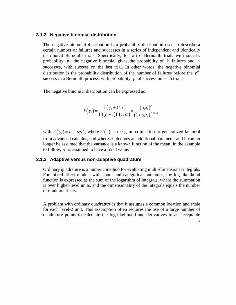
3.1.2 Negative binomial distribution

The negative binomial distribution is a probability distribution used to describe a certain number of failures and successes in a series of independent and identically distributed Bernoulli trials. Specifically, for k r Bernoulli trials with success probability p , the negative binomial gives the probability of k failures and r successes, with success on the last trial. In other words, the negative binomial distribution is the probability distribution of the number of failures before the thr success in a Bernoulli process, with probability p of success on each trial.

The negative binomial distribution can be expressed as

1/

1/

1 1/ 1

i

i

y

i ii y

i i

yf y

y

with 2i i iy , where is the gamma function or generalized factorial

from advanced calculus, and where denotes an additional parameter and it can no longer be assumed that the variance is a known function of the mean. In the example to follow, is assumed to have a fixed value.

3.1.3 Adaptive versus non-adaptive quadrature

Ordinary quadrature is a numeric method for evaluating multi-dimensional integrals. For mixed-effect models with count and categorical outcomes, the log-likelihood function is expressed as the sum of the logarithm of integrals, where the summation is over higher-level units, and the dimensionality of the integrals equals the number of random effects.

A problem with ordinary quadrature is that it assumes a common location and scale for each level-2 unit. This assumption often requires the use of a large number of quadrature points to calculate the log-likelihood and derivatives to an acceptable

8

level of accuracy. To overcome this problem with ordinary quadrature, SuperMix also offers a numeric integration procedure called adaptive quadrature. The adaptive quadrature procedure uses the empirical Bayes means and covariances, updated at each iteration to essentially shift and scale the quadrature locations of each higher-level unit in order to place them under the peak of the corresponding integral. To distinguish between the two quadrature methods, SuperMix uses the terminology non-adaptive quadrature (ordinary quadrature) and adaptive quadrature. To illustrate this, models in Section 3.2 will be fitted using adaptive quadrature, while models in Section 3.3 will use the default method of non-adaptive quadrature.

9

3.2 Two-level models for count outcomes from NESARC data

3.2.1 The data

The data set is from the National Epidemiologic Survey on Alcohol and Related Conditions (NESARC), which was designed to be a longitudinal survey with its first wave fielded in 2001-2002. This data file has been used in some of the examples in Chapter XXX. Detailed information about the survey is available at http://niaaa.census.gov/index.html.

In Section 4 of the description of the NESARC study, information on the data regarding occurrences of major depression, family history of major depression and dysthymia are collected. This information was used, in combination with the demographic information provided in Section 1 of the study description, to produced the nesarc_poi.ss3 data set used in this section. The image below shows the first ten records of this data set. There are 2339 dysthymia respondents in the survey; after listwise deletion, the sample size is 1981.

10

The variables of interest are:

o PSU denotes the Census 2000/2001 Supplementary Survey (C2SS) primary sampling unit.

o FINWT represents the NESARC weights sample results used to form national level estimates. The final weight is the product of the NESARC base weight and other individual weighting factors.

o CONC_DEP contains the information captured in field S4CQ3A6 of the NESARC data. It represents the response to the statement "Often had trouble concentrating/keeping mind on things," with 1 indicating "Yes," and 0 indicating "No."

o AGE_DEP is based on field S4CQ7AR of the NESARC data. It represents the age at onset of first episode.

o N_DEP is recoded from field S4CQ6A of the NESARC data, and gives the number of depression/dysthymia episodes. This is the count variable we would like to use as outcome variable in the examples to follow.

3.2.1.1 Exploring the data

Inspecting the distribution of the intended outcome variable, N_DEP, before starting with the model is important. In the case of a count variable, this can easily be done by producing a bar chart of the observed frequencies of occurrence captured by the count variable. Select the File, Data-based Graph, Univariate option from the main SuperMix window and request a bar chart before clicking the Plot button.

11

Figure XXX.3: Bar chart for count variable N_DEP

The frequency bar chart for the count variable N_DEP shown in Figure XXX.3 is obtained. We note that the number of depression episode ranges from 1 to 29, with most respondents having a small number of reported episodes of depression.

3.2.2 A 2-level Poisson model with 2 predictors

3.2.2.1 The model

The first model fitted to the data explores the relationship between N_DEP and the variables indicating concentration (or lack thereof) and age, as represented by the variables CONC_DEP and AGE_DEP.

The level-1 model is

0 1 2log CONC_DEP AGE_DEPij ij ij

where the expected number of depression episodes is =E N_DEPij ij .

12

The level-2 model is

0 00 0ib v , 1 10b and 2 20b .

Another way of writing the combined model is

00 10 20 0log CONC_DEP AGE_DEPij ij ij ib b b v .

In this model, 00be denotes the average expected count of depression episodes, and

10b represents the estimated coefficient for the respondent's level of concentration.

Taking exponents on both sides, we also have

00 10 20 0

10 2000 0

ij ij i

ij ij i

b b b vij

b bb v

e

e e e e

CONC_DEP AGE_DEP

CONC_DEP AGE_DEP

For a person who had problems concentrating (CONC_DEP = 1), the expected average number of episodes 00be is multiplied by 1e , compared to an expected count of 00be for a person for whom CONC_DEP = 0. Similarly, an increase of one year in age increases the estimated number of episodes by a factor of 20be . For example, a respondent with concentration problems who is two years older than another respondent who had no concentration problems is expected to have

00 10 202b b be e e episodes compared to only 00be episodes for the younger person without concentration problems.

The random part of the model is represented by 0ive , which denotes the variation in average count of depression episodes over PSU and between respondents (or, in other words, over respondents nested within PSU). For a Poisson distribution, the assumption of normality at level 1 is not realistic, as the level-1 random effect can

13

only assume a number of distinct values. Thus, this random effect cannot have homogeneous variance.

3.2.2.2 Setting up the analysis

Open the SuperMix spreadsheet nesarc_poi.ss3 used during the exploratory analysis. From the main menu bar, select the File, New Model Setup option. The Model Setup window that appears has six tabs. In this example, only three tabs are used: the Configuration, Variables, and Advanced tabs.

The Configuration screen is the first tab on the Model Setup window. It enables the user to define the outcome variable and the level-2 and level-3 IDs. Some other settings such as missing values, convergence criterion, number of iterations, etc. can be specified here. For all the available settings, please refer to chapter XXXX. To obtain the model we discussed, start by selecting the outcome variable N_DEP from the Dependent Variable drop-down list box. Indicate that it is a count variable by selecting the count option from the Dependent Variable Type drop-down list box. Next, describe the hierarchical structure of the data by selecting the level-2 ID, PSU,

14

from the Level-2 IDs drop-down list box. Enter a title in the Title text boxes, and proceed to the Variables screen by clicking on this tab.

The Variables screen is used to specify the fixed and random effects to be included in the model. To include the variables CONC_DEP and AGE_DEP as predictor variables, check the E check boxes next to the variables' names. Note that, as the variables are selected, the selected variables are listed in the Explanatory Variables grid. After selection, the screen below is obtained. Note that the Include Intercept check boxes in the Explanatory Variables grid and L-2 Random Effects are checked by default, indicating that an intercept term will automatically be included in the fixed and random parts of the model.

As mentioned previously, the models based on the NESARC data are fitted using adaptive rather than full quadrature. The final step of model specification is to request the use of adaptive quadrature, and this is done on the Advanced tab.

15

Click on the Advanced tab, and request adaptive quadrature using the Optimization Method drop-down list box. Do not change the number of quadrature points from the default displayed (10).

Before running the analysis, the model specifications have to be saved. Select the File, Save As option, and provide a name (nesarc_poi1.mum) for the model specification file. Run the analysis by selecting the Run option from the Analysis menu.

3.2.2.3 Discussion of results

Portions of the output file nesarc_poi.out are shown below.

Program information and syntax

As shown below, the syntax for the model setup is printed in the output file. The first line of the syntax shows the option Model = Count, which indicates the outcome variable is a count variable. The Options syntax line corresponds to the settings on

16

the Configuration screen. The Link = log and Distribution = Poi options specify the use of a Poisson distribution with a log link function for the fitted model.

Data summary

A description of the hierarchical structure follows the syntax: data from a total of 395 PSU and 1981 respondents were included at levels 2 and 1 of the model. In

17

addition, an enumeration of the number of respondents nested within each of the 395 PSUs is provided.

Descriptive statistics

The data summary is followed by descriptive statistics for all the variables included in the model. The mean of 1.8970 and standard deviation of 2.3304 are reported for the outcome N_DEP indicating that, on average, 1.8970 episodes of depression were recorded.

Descriptive statistics are followed by the results for a fixed-effects-only model, i.e. a model without random coefficients.

Fixed effects results

At the top of the final results, the number of iterations required for convergence of the iterative procedure is given. Next, the number of quadrature points per dimension is reported which, in this case, is the default number of points. The log likelihood and the deviance, which is defined as 2ln L , are listed next. For a pair of nested models, the difference in 2ln L values has a 2 distribution, with degrees of freedom equal to the difference in number of parameters estimated in the models compared.

18

The estimated intercept is 0.7982, which means that the average number of depression episodes is 0.7982e =2.2215 , implying that on average the number of episodes is about two. The estimated coefficient for CONC_DEP is 0.2922, which indicates that respondents who had trouble concentrating on things tended to have

0.29222.2215e = 2.2215 1.3394 =2.9754 episodes at the same age as respondents

without concentration problems. The estimate of the effect of age at the onset of the first episode (AGE_DEP) shows that the onset age does not affect the number of episodes much, since -0.0165e = 0.98 . A slight reduction in the expected number of episodes is expected with increasing age. If one compares two typical respondents with reported concentration problems, but with one respondent ten years older than the other, one would expect the older respondent to have

10(-0.0165)e2.2215 1.3394 =2.5229 episodes, compared to 2.9268 expected episodes

for the younger respondent. In other words, the longer it takes for the first episode to occur, the fewer episodes a respondent is expected to have. Of course, it has to be kept in mind that the younger a respondent is at the first episode, the longer that

19

person must live with the condition and thus the more time there is for subsequent episodes to occur.

Random effects results

The output for the level-2 random effect variance term follows next. The estimated variation in the average estimated N_DEP at level 2 is 0.1347, which is highly significant. Respondents are different in terms of their average expected number of episodes, holding all other variables constant.

Level-1 variation for Poisson distribution

The variance-to-mean ratio is a measure of the dispersion of a probability distribution:

2

variance-to-mean ratioR

For the Poisson distribution, where the variance equals the mean, this implies 1R . Thus, we use a value of one as our level-1 variation. In the cases when over-dispersion ( 1R ) or under-dispersion ( 1R ) is assumed, different level-1 variation values will apply. The details of these scenarios are not discussed in this guide. Please refer to XXXXX for more details.

20

3.2.2.4 Interpreting the results

Estimated outcomes for groups: unit-specific results

First, we substitute the regression weights and obtain the following function for log N_DEPij :

10 2000ˆlog N_DEP CONC_DEP AGE_DEP

0.7982 0.2922 CONC_DEP 0.0165 AGE_DEP .

ij ijij

ij ij

b b b

For example, at age 40, the estimated log N_DEPij for a typical respondent who

does not often have trouble concentrating (CONC_DEP = 0), we find that

00 1 2ˆ ˆ ˆlog N_DEP CONC_DEP AGE_DEP

0.7982 0.2922 CONC_DEP 0.0165 AGE_DEP

0.7982 0.2922 0 0.0165 40

0.1382.

ij ijij

ij ij

b

Keeping in mind that we defined the relationship between and the predictors as

1 1log ij i p ipx x ,

it follows that

0.1382ˆ 1.1482.ij e

21

We can estimate the count of the occurrence of depression episodes for typical individuals of different ages in the same way. Results are summarized in Table XXX.1. The results show a decrease in the expected number of episodes with increasing age, regardless of whether they had concentration problems or not.

Table XXX.1: Estimated number of episodes under the Poisson log model

AGE_DEP 10 20 30 40 50 60 70

CONC_DEP = 1 2.5229 2.1391 1.8138 1.5379 1.3040 1.1056 0.9374

CONC_DEP = 0 1.8836 1.5971 1.3542 1.1482 0.9736 0.8255 0.6999

The results in Table XXX.1 can also be presented graphically, as shown in Figure XXX.4. We clearly see that the correspondents who often had trouble concentrating (CONC_DEP = 1) have a higher estimated number of depression episodes. It also shows that the number of episodes is expected to decrease as people get older.

Figure XXX.4: Expected number of episodes for two groups

22

Level 2 ICC

The percentage of variance explained over level-2 units, or intraclass correlation coefficient (ICC), is calculated as

level-2 variation

level-1 variation + level-2 variation ICC

In this example, under the assumption that the level-1 variation is fixed at a value of one, we have

0.1347100% 11.8%

1 + 0.1347 ICC

We can conclude that most of the unexplained variation in the outcome (approximately 78%) is between measurements at the lowest level of the hierarchy.

3.2.3 A 2-level negative binomial model with 2 predictors

3.2.3.1 The model

In Section 3.2.2, a Poisson model was fitted to the data. It was also noted that a Poisson distribution has an important property: the mean number of occurrences is equal to the variance. The negative binomial distribution is an alternative distribution that may also be used to describe the properties of count variables. If the assumption of a Poisson distribution is reasonable, one would expect a model using a negative binomial distribution with a very small dispersion parameter to produce results that correspond closely to those obtained for the Poisson model. In this section, we fit a negative binomial model, utilizing the same predictors and a small dispersion parameter, to the NESARC data. Again, adaptive quadrature is used as the method of optimization.

23

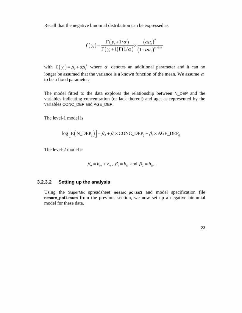
Recall that the negative binomial distribution can be expressed as

1/

1/

1 1/ 1

i

i

y

i ii y

i i

yf y

y

with 2i i iy where denotes an additional parameter and it can no

longer be assumed that the variance is a known function of the mean. We assume to be a fixed parameter.

The model fitted to the data explores the relationship between N_DEP and the variables indicating concentration (or lack thereof) and age, as represented by the variables CONC_DEP and AGE_DEP.

The level-1 model is

0 1 2log E N_DEP CONC_DEP AGE_DEPij ij ij

The level-2 model is

0 00 0ib v , 1 10b and 2 20b .

3.2.3.2 Setting up the analysis

Using the SuperMix spreadsheet nesarc_poi.ss3 and model specification file nesarc_poi1.mum from the previous section, we now set up a negative binomial model for these data.

24

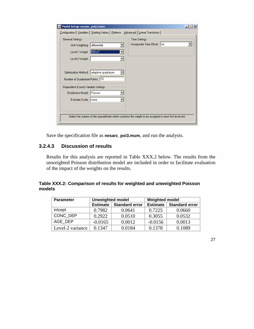
Start by saving the model specification file under the new name nesarc_poi2.mum using the File, Save As option. Next, click on the Advanced tab of the Model Setup window. This is the only tab on which modifications have to be made to change the previously specified Poisson model to a negative binomial model. Set the Distribution Model to negative binomial, and the Dispersion Parameter to 0.0001 to obtain an Advanced tab as shown below. Also, request adaptive quadrature using the Optimization Method drop-down list box. Do not change the number of quadrature points from the default displayed (10).

Save the revised model specification file, and click the Analysis, Run option to start the iterative process.

25

3.2.3.3 Discussion of results

Portions of the output file nesarc_poi.out are shown below.

Fixed and random effect results

The estimated regression coefficients for fixed effects in the model are shown below. Recall that the estimated coefficients of the intercept, CONC_DEP, and AGE_DEP under the Poisson model in Section 3.2.2 were 0.7982, 0.2922, and

0.0165 respectively. The estimated variation in the average estimated N_DEP at level-2 was 0.1347, and highly significant. The similarity of the results obtained under these two models indicate that the specification of a Poisson distribution model is reasonable for this data.

26

3.2.4 Weighted 2-level models

3.2.4.1 The data

The sampling frame of many multistage surveys frequently entails selection of units with known, but unequal, selection probabilities. This situation is the result of a number of design factors, of which the cost of doing the survey is an important consideration. When this is the case, it is appropriate to weight observations in order to produce unbiased estimates of population parameters.

Recall from Section 3.2.1 that the data also included a weight variable. The variable FINWT represents the NESARC weights sample results used to form national-level estimates. The final weight is the product of the NESARC base weight and other individual weighting factors. In this section, we explore the effect of inclusion of the weights on the results obtained in Sections 3.2.2 and 3.2.3.

3.2.4.2 Setting up the analysis

The models remain the same, with only the selection of the weight variable on the Advanced tab of the Model Specification screen to be added. Below, we show how this is done in the case of the Poisson distribution model.

Open the model specification file for the Poisson distribution model (nesarc_poi1.mum) and click on the Advanced tab. Change the Unit Weighting field from its default value of equal to differential. Next, select the variable FINWT from the Assigned Weight drop-down list box that appears when the selection has been made in the Unit Weighting field. The completed Advanced tab is shown below.

27

Save the specification file as nesarc_poi3.mum, and run the analysis.

3.2.4.3 Discussion of results

Results for this analysis are reported in Table XXX.2 below. The results from the unweighted Poisson distribution model are included in order to facilitate evaluation of the impact of the weights on the results.

Table XXX.2: Comparison of results for weighted and unweighted Poisson models

Unweighted model Weighted model Parameter Estimate Standard error Estimate Standard error

intcept 0.7982 0.0641 0.7225 0.0660 CONC_DEP 0.2922 0.0510 0.3055 0.0532 AGE_DEP -0.0165 0.0012 -0.0156 0.0013 Level-2 variance 0.1347 0.0184 0.1378 0.1089

28

Results for the two models are very similar, and interpretation of the results of both models would lead to the same conclusions, both in terms of significance and in terms of the expected number of depression episodes. However, this is more the exception than the rule – users are cautioned to use weight variables whenever they are available in order to prevent skewed or biased results that may occur when weights are excluded in the analysis of a disproportionally drawn sample.

29

3.3 Two-level models for count outcomes from ASPART data

3.3.1 The data

The data for this example are taken from a paper by McKnight and Van Den Eeden (1993), who reported on the number of headaches in a two treatment, multiple period crossover trial. Specifically, the number of headaches per week was repeatedly measured for 27 patients. Following a seven day placebo run-in period, subjects received either aspartame or placebo in four seven-day treatment periods according to the double-blind crossover treatment design. Each treatment period was separated by a washout day. The sample size is 122. Data for the first 10 observations of all the variables used in this section are shown below in the form of a SuperMix spreadsheet window for aspart.ss3.

The variables of interest are:

o ID is the patient ID (27 patients in total).

o Headache is the number of headaches during the week (from 0 to 7).

o Period1 is a period 1 treatment indicator (1 for the first treatment period and 0 otherwise).

o Period2 is a period 2 treatment indicator (1 for the second treatment period and 0 otherwise).

30

o Period3 is a period 3 treatment indicator (1 for the third treatment period and 0 otherwise).

o Period4 is a period 4 treatment indicator (1 for the fourth treatment period and 0 otherwise).

o DrugAsp indicates the type of drug being used for the treatment, (0 = placebo and 1 = aspartame). 75 observations used placebo and 47 used aspartame.

o Nperiods is the number of periods the individual was observed (from 2 to 5).

o NTDays is the number of treatment days in the period (from 1 to 7).

3.3.2 A 2 level Poisson model with random intercept

3.3.2.1 The model

To model the relationship between the number of headaches during the week (Headache) and the treatment indicators (Period1 to Period4) and the type of drug administered (DrugAsp), the following Poisson regression model with a random intercept may be used:

0 1 2 3

4 5 0

log Period1 Period2 Period3

Period4 DrugAsp

ij ij ij ij

ij ij iv

where ij denotes the estimated mean number of headaches of patient i for

treatment period j ; ijPeriod1 , ijPeriod2 , ijPeriod3 and ijPeriod4 denote the values of

the dummy variables Period1, Period2, Period3 and Period4 for patient i for treatment period j respectively; ijDrugAsp denotes the value of the DrugAsp for patient i for

treatment period j ; 0 , 1 , 2 , 3 , 4 and 5 denote unknown parameters; and

0iv denotes the random intercept for patient i for 1, 2, , 27i and 0,1, 2,3j .

This model is fitted to the data in aspart.ss3 as described below.

31

3.3.2.2 Setting up the analysis

Start by opening the SuperMix spreadsheet aspart.ss3. Select the New Model Setup option on the File menu to load the Model Setup window. On the Configuration tab, enter the titles 2 level Poisson log random intercept model and ASPART data for the analysis in the Title 1 and Title 2 text boxes respectively. The count outcome variable Headache is selected from the Dependent Variable drop-down list box. The Dependent Variable Type drop-down list box is used to indicate that the outcome variable is a count. The variable ID, which defines the levels of the hierarchy, is selected as the Level-2 ID from the Level-2 IDs drop-down list box.

Next, click on the Variables tab to proceed with variable selection. The variables Period1, Period2, Period3, Period4, and DrugAsp are specified as the fixed effects of the model by checking the E check boxes for Period1, Period2, Period3, Period4, and DrugAsp in the Available grid. These actions produce the following Variables tab. By

32

default, an intercept model is included in the fixed part of the model, along with a random intercept at level 2.

Finally, we click on the Advanced screen and keep all the default settings as shown below, except for the quadrature points which are set to 20. Before we can run the analysis, we have to save the model specifications to a file. This is accomplished by using the Save option on the File menu to open a Save Mixed Up Model dialog box. First enter the name aspart1.mum in the File name text box and then click on the Save button to save the file. The analysis is run by selecting the Run option from the Analysis menu. This produces the corresponding output file aspart1.out.

33

3.3.2.3 Discussion of results

Portions of this output file are shown below.

Data summary

34

The output file indicates that there are 27 subjects with 122 observations nested within them. The number of observations per subject varies between 2 and 5.

Descriptive statistics and starting values

The descriptive statistics for all the variables is shown next. The variance of Headache is 21.8863 3.5581 , which is substantially larger than the mean 1.6803. This might conflict with our assumption that the Poisson distribution is an appropriate choice for these data. As pointed out in Section 3.2.3, this can be verified by fitting a negative binomial model with a small dispersion parameter.

The starting values are given next.

35

Following the listing of the starting values, SuperMix indicates that of the 27 subjects, 2 had response vectors that were non-varying. Thus, 2 subjects gave identical responses at all time points that they were measured on.

Fixed and random effect results

The final results are shown next. The number of iterations needed for convergence and the deviance information are given first, followed by the estimates.

The random-effect standard deviation is estimated as .643, and although a Wald test rejects the hypothesis that this parameter equals 0, use of the Wald test for testing whether variance parameters equal zero is questionable, since the Wald test is based on the assumption that parameters can assume any real value. Regarding the regression coefficients, all effects are non-significant. The results indicate that the model does not fit the data very well.

36

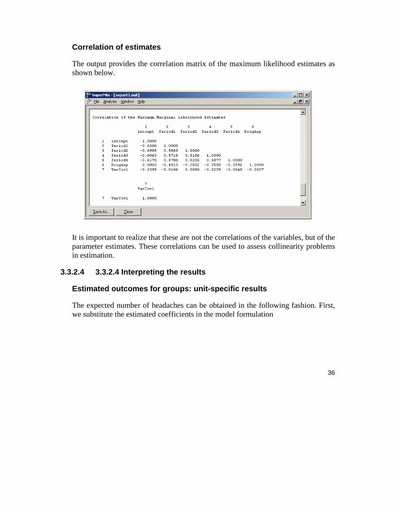
Correlation of estimates

The output provides the correlation matrix of the maximum likelihood estimates as shown below.

It is important to realize that these are not the correlations of the variables, but of the parameter estimates. These correlations can be used to assess collinearity problems in estimation.

3.3.2.4 3.3.2.4 Interpreting the results

Estimated outcomes for groups: unit-specific results

The expected number of headaches can be obtained in the following fashion. First, we substitute the estimated coefficients in the model formulation

37

0 1 2

3 4 5

log Headache Period1 Period2

Period3 Period4 DrugAsp

0.24035 0.08031 Period1 0.03412 Period2

0.22923 Period3 0.16071 Period4 0.21536 DrugAsp .

ij ij ij

ij ij ij

ij ij

ij ij ij

or, after taking exponents on both sides, as

Headache exp(0.24035 0.08031 Period1 0.03412 Period2

0.22923 Period3 0.16071 Period4 0.21536 DrugAsp ).

ij ij ij

ij ij ij

As an example, we calculate the expected number of headaches for a typical patient to whom aspartame was administered (DrugAsp = 1).

During the first treatment period, we find that for such a patient

Headache exp(0.24035 0.08031 0.21536)

1.7092.

ij

The expected numbers of headaches for a typical patient (again with DrugAsp = 1) for the second, third, and fourth treatment periods are calculated as

Headache exp(0.24035 0.03412 0.21536)

1.6320,

ij

Headache exp(0.24035 0.22923 0.21536)

1.2542,

ij

38

and

Headache exp(0.24035 0.16071 0.21536)

1.3431

ij

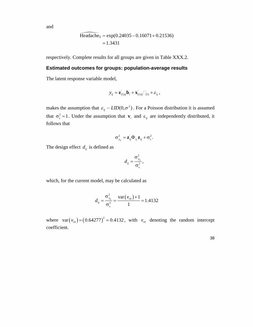
respectively. Complete results for all groups are given in Table XXX.2.

Estimated outcomes for groups: population-average results

The latent response variable model,

' '

(1) (1) (1)ij ij i ij ijy z b x â ,

makes the assumption that 2(0, )ij LID . For a Poisson distribution it is assumed

that 2 1 . Under the assumption that iv and ij are independently distributed, it

follows that

2 ' 2.

ij iy ij v ij z z

The design effect ijd is defined as

2

2,ijy

ijd

which, for the current model, may be calculated as

2

02

var 11.4132

1ijy i

ij

vd

where 2

0var 0.64277 0.4132iv , with 0iv denoting the random intercept

coefficient.

39

The estimated population-average probabilities (Hedeker & Gibbons, 2006) are obtained in a similar fashion as the unit-specific probabilities, after replacing the exponent in the formula used for calculation of the estimated unit-specific

probabilities with exp exp/ ijd as shown below.

Headache exp[(0.24035 0.08031 Period1 0.03412 Period2

0.22923 Period3 0.16071 Period4

0.21536 DrugAsp ) / 1.4132].

ij ij ij

ij ij

ij

The expected unit-specific and population average probabilities are summarized in Table XXX.2. We see that there is very little difference in the estimated number of

headaches. This result is to be expected as the design effect is 1.4132 1.1888 .

Table XXX.2: Estimated unit-specific and population average results for groups

DRUGASP Period Estimated headaches

(unit-specific)

Estimated headaches

(population-average)

0 1 1.3780 1.3096

0 2 1.3158 1.2597

0 3 1.0112 1.0094

0 4 1.0829 1.0693

1 1 1.7092 1.5697

1 2 1.6320 1.5099

1 3 1.2542 1.2099

1 4 1.3431 1.2817

40

3.3.3 A 2-level Poisson log model with an offset variable

3.3.3.1 The model

The previous analysis assumed that the counts were all observed for the same number of days. However, this was not the case since the number of treatment days in the period did vary to some degree. Most of the counts were based on the full seven days in the week; however, some observations were made only for 1 day in the given week. To take this into account, we need to specify a so-called OFFSET variable. The offset variable indicates the amount of time that each count is based on. If OFFSET = no is specified, as was the case in the previous example, SuperMix assumes that all counts are based on the same amount of time.

The offset variable is introduced into the Poisson model in the following way:

'log log(offset variable)ij ij i x b

where ijx represent the values of the covariates corresponding to level-1 unit j

nested within level-2 unit i and ib denotes the coefficient vector containing both

fixed and random effects.

In the current situation, the variable NTDays is the appropriate choice as the OFFSET variable. The model to be fitted to the data now changes to:

0 1 2

3 4 5 0

log Headache log NTDays ( Period1 Period2

Period3 Period4 DrugAsp ).

ij ij ij

ij ij ij iv

41

3.3.3.2 Setting up the analysis

To create the model specifications for this model, start by opening aspart.ss3 in a SuperMix spreadsheet window and using the Open Existing Model Setup option on the File menu to open the Model Setup window for aspart1.mum. On the Configuration screen, extend the title in the Title 1 text box by adding the string "with Offset Variable." Next, click on the Advanced tab of the Model Setup window. Select yes from the Incorporate Time Offset drop-down list to activate the Offset Variable drop-down list box. Select the variable NTDays from the drop-down list of Offset Variable to produce the following Advanced tab.

Save the changes to the file aspart2.mum by using the Save As option on the File menu and select the Run option on the Analysis menu to produce the output file aspart2.out.

42

3.3.3.3 Discussion of results

Fixed and random effect results

A portion of this output file is shown below.

Results for this model differ from those obtained for the model without offset variable discussed in the previous Section. While the overall trend in predictor coefficient estimates is similar, the intercept is now estimated as -1.45244, compared to 0.24035 previously. The variance in intercept over patients for this

model is estimated as 21.07699 1.1599 compared to 2

0.6428 0.4132

previously.

43

3.3.3.4 3.3.3.4 Interpreting the results

Estimated outcomes for groups: unit-specific results

The expected number of headaches can be obtained in the following fashion. First, we substitute the estimated coefficients in the model formulation

0 1 2

3 4 5

log Headache log NTDays ( Period1 Period2

Period3 Period4 DrugAsp )

log NTDays ( 1.45244 0.11789 Period1 0.10988 Period2

0.16975 Period3 0.04373 Period4 0.28106 Dr

ij ij ij ij

ij ij ij

ij ij ij

ij ij

ugAsp ),ij

or, after taking exponents on both sides, as

Headache NTDays exp( 1.45244 0.11789 Period1 0.10988 Period2

0.16975 Period3 0.04373 Period4 0.28106 DrugAsp ).

ij ij ij ij

ij ij ij

As most observations had a value of NTDays = 7, we start by considering typical patients with a full set of treatment days. We also assume that DrugAsp = 1, in other words, that aspartame rather than a placebo was administered.

During the first treatment period, we find that for such a patient

Headache 7 exp( 1.45244 0.11789 0.28106)

7 exp( 1.05349)

2.4410.

ij

The expected numbers of headaches for a typical patient (again with NTDays = 7 and DrugAsp = 1) for the second, third, and fourth treatment periods are calculated as

44

Headache 7exp( 1.45244 0.10988 0.28106)

2.4216,

ij

Headache 7exp( 1.45244 0.16975 0.28106)

1.8308,

ij

and

Headache 7exp( 1.45244 0.04373 0.28106)

2.0767

ij

respectively.

For a typical patient with only 5 treatment days, the expected numbers of headaches in each of the four treatment periods are 1.7436, 1.7297, 1.3077, and 1.4834 respectively.

When the expected numbers of headaches for a typical patient receiving aspartame under the Poisson model without offset variable (see previous Section) and the Poisson model with offset variable are compared, we clearly see the impact of the inclusion of the offset variable on the estimated coefficients. These results are summarized in Table XXX.3.

Table XXX.3: Comparison of results for Poisson models

Period Without offset variable

With offset variable

(NTDays = 7)

With offset variable

(NTDays = 5)

1 2.3553 2.4410 1.7436

2 1.6320 2.4216 1.7297

3 1.2542 1.8308 1.3077

4 1.3431 2.0767 1.4834

45

Level 2 Bayes results

As requested during the model specification stage, the empirical Bayes estimates of the random effects are written to the file aspart2.ba2. The first few lines of this file are shown below.

The file mixreg.ba2 contains five pieces of information per individual:

o the individual's ID,

o the number of repeated observations for that individual,

o the empirical Bayes estimate for that individual (which is the mean of the posterior distribution),

o the associated posterior standard deviation, and

o the name of the relevant random coefficient.

Since they are estimates of 0ib for each individual, the empirical Bayes estimates

are expressed on the standard normal scale. Inspection of these estimates indicates

46

that subject 13 has a very high score. This person's estimate of 1.043 (with standard deviation .016) suggests a very high level of headaches. This agrees well with the raw data, which reveals that this person recorded 7 headaches on four occasions and 6 on the only other occasion.

Graphical displays

Figure XXX.5 is a comparison (represented by a dotted line) of the predicted average number of headaches reported by each patient when taking a placebo (left axis) as opposed to the predicted average number when the treatment is aspartame (right axis). From the graphical display, it appears as if all of the lines (each representing a patient) have a positive slope. The slopes become steeper as the number of headaches increases. This suggests an increase, albeit small, in the expected average number of headaches when aspartame is used. Note that patient 13, who reported a consistently high number of headaches at all occasions, was excluded from this graph.

Figure XXX.5: Predicted average number of headaches for placebo and aspartame

47

48

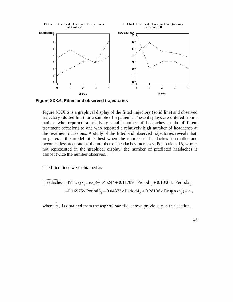
Figure XXX.6: Fitted and observed trajectories

Figure XXX.6 is a graphical display of the fitted trajectory (solid line) and observed trajectory (dotted line) for a sample of 6 patients. These displays are ordered from a patient who reported a relatively small number of headaches at the different treatment occasions to one who reported a relatively high number of headaches at the treatment occasions. A study of the fitted and observed trajectories reveals that, in general, the model fit is best when the number of headaches is smaller and becomes less accurate as the number of headaches increases. For patient 13, who is not represented in the graphical display, the number of predicted headaches is almost twice the number observed.

The fitted lines were obtained as

0

Headache NTDays exp( 1.45244 0.11789 Period1 0.10988 Period2

0.16975 Period3 0.04373 Period4 0.28106 DrugAsp ) .

ij ij ij ij

iij ij ij b

where 0ib is obtained from the aspart2.ba2 file, shown previously in this section.

49

References

McKnight and Van Den Eeden (1993)