3 experimental designs

5/20/2015-1

Experimental Designs

5/20/2015-2

Experimental Design Overview

• Experimental Design Types– Factorial designs and fractional factorial designs– Response surface methodology– Optimal designs– Restricted randomization designs

» Blocking» Split-plots

• Design Evaluation– Statistical measures of merit

• Designs for Software Testing

5/20/2015-3

Steps in Designing an Experiment

1. Define the objective of the experiment

2. Select appropriate response variables

3. Choose factors, levels

4. Choose experimental design – Disallowed combinations of factors

(safety, operational realism)– Realistic range for test resources– Allowable test risk– Analysis objectives

5. Perform the test

6. Statistically analyze the data

7. Draw conclusions

Steps are strategically linked into a defensible process.

5/20/2015-4

Motivating Example: Test Plan for Mine Susceptibility

• Goal:– Develop an adequate test to assess the susceptibility of a cargo

ship against a variety of mine types using the Advanced Mine Simulation System (AMISS).

• Responses:– Magnetic signature, acoustic signature, pressure– Slant range at simulated detonation

• Factors:– Speed, range, degaussing system status

• Other considerations:– Water depth– Ship direction

5/20/2015-5

Test Designs

Low HighMedium

Low

Medium

High

One run with degaussing, one without degaussing

Hor

izon

tal R

ange

Speed

2

22

2

Design Type Number of Runs

Full Factorial (2-level) 8

Fractional Factorial Design 4

Full Factorial Design (with center point) 10

Full Factorial (2-level) replicated 16

General Factorial (3x3x2) 18

Response Surface Design: Central Composite Design 18

Central Composite Design (replicated center point) 20

Central composite Design with replicated factorial points (Large CCD)

28

Optimal DesignVaries with

model selected

5/20/2015-6

Test Designs

Low HighMedium

Low

Medium

High


Hor

izon

tal R

ange

Speed

2

22

2

Full Factorial Designs (2 – level)

• A design with two or more factors, each with two levels, where all possible factor combinations are tested at least once.

• Typically used in DT and OT when the total number of factors and factor combinations is not too large (e.g., 3-5 factors).

• A full factorial design allows for the estimation of all main effects and interaction terms in the model.

• Full factorial designs tend to provide too much information (over powered) for large numbers of factors.

5/20/2015-7

Test Designs

Low HighMedium

Low

Medium

High

Hor

izon

tal R

ange

Speed

1

11

1










28


model selected

With Degaussing

Without Degaussing

5/20/2015-8

Test Designs

Low HighMedium

Low

Medium

High

Hor

izon

tal R

ange

Speed

1

11

1

With Degaussing

Without Degaussing

Fractional Factorial Designs

• A fractional factorial design consists of a strategically selected subset of runs from a full factorial design

• Useful when:• Large number of factors and it is

uneconomical to test every possible factor combination

• In screening experiments to identify the primary factors

• Typically, fractional factorial designs that allow for two-way interactions are adequate to characterize system performance

• Leverages sparsity of effects: most systems are dominated by some of the main effects and low order interactions

5/20/2015-9

Test Designs

Low HighMedium

Low

Medium

High


Hor

izon

tal R

ange

Speed

2

22

2










28


model selected

2

5/20/2015-10

Test Designs

Low HighMedium

Low

Medium

High


Hor

izon

tal R

ange

Speed

2

22

2

2

Center Points

• Add the ability to check for curvature across continuous factors

• Provide small increases to statistical power

5/20/2015-11

Test Designs

Low HighMedium

Low

Medium

High

Two runs with degaussing, two without degaussing

Hor

izon

tal R

ange

Speed

4

44

4










28


model selected

5/20/2015-12

Test Designs

Low HighMedium

Low

Medium

High

Two runs with degaussing, two without degaussing

Hor

izon

tal R

ange

Speed

4

44

4

Replication

• Can be used to increase statistical power

• Provide estimates of variation within a condition

• Often not possible in cost constrained operational tests

• In a constrained resource environment it is better to cover more of the operational space than to replicate (i.e., do not eliminate a factor for the sake of replication)

• A common middle ground is to only replicate a subset of the design (e.g., a center point)

5/20/2015-13

Test Designs

Low HighMedium

Low

Medium

High

Hor

izon

tal R

ange

Speed

2

22

2 2

222

2










28


model selected

5/20/2015-14

Test Designs

Low HighMedium

Low

Medium

High

Hor

izon

tal R

ange

Speed

2

22

2 2

222

2

General Factorial Designs

• Similar to a two-level factorial design, designs with two or more factors, each with two or more levels, where all possible factor combinations are tested at least once.

• Only possible when the number of factors is not too large (e.g., 3-5 factors).

• Allows for the estimation of all main effects and interaction terms in the model.

• Less powerful as you add more levels to each factor

• For continuous factors, two-levels provides the highest power

5/20/2015-15

Test Designs

Low HighMedium

Low

Medium

High

Hor

izon

tal R

ange

Speed

2

22

2

2

222

2










28


model selected

5/20/2015-16

Test Designs

Low HighMedium

Low

Medium

High

Hor

izon

tal R

ange

Speed

2

22

2

2

222

2

Response Surface Designs

• Response Surface Methodology is a collection of experimental designs

– Originally invented by the chemical industry to conduct sequential experimentation for process optimization

– Evolved to be a broad class of designs that characterize system performance

– Robust test design methodology fits second order models including quadratic effects for flexible performance characterization

• Types of Response Surface Designs:– Central Composite Design, Face

Centered Cube Design, Small Central Composite Design, Box-Behnken Designs, Optimal Designs

5/20/2015-17

Test Designs

Low HighMedium

Low

Medium

High

Hor

izon

tal R

ange

Speed

2

22

2

2

242

2










28


model selected

5/20/2015-18

Test Designs

Low HighMedium

Low

Medium

High

Hor

izon

tal R

ange

Speed

4

44

4

2

242

2










28


model selected

5/20/2015-19

Test Designs

Low HighMedium

Low

Medium

High

Hor

izon

tal R

ange

Speed

2










28


model selected

Disallowed Combination

With Degaussing

Without Degaussing

2

5/20/2015-20

Test Designs

Low HighMedium

Low

Medium

High

Hor

izon

tal R

ange

Speed

2

Disallowed Combination

With Degaussing

Without Degaussing

2

Optimal Designs

• Optimize the test points for a known analysis model and sample size

• Optimal designs are useful:– Large number of factors– Highly constrained design region

(disallowed combinations of factors)– Large number of categorical factors

• The optimal design fallacy– Designs that are optimal under one

criteria might be far from optimal under another criteria

• Optimal designs are similar to factorial designs and response surface designs for similar analysis models

• Always build in extra points to optimal designs to allow for incorrect model assumptions and statistical power

5/20/2015-21

General Factorial3x3x2 design

2-level Factorial23 design

Fractional Factorial23-1 design

Response SurfaceCentral Composite design

A Structured Approach to Picking Test Points(Tied to Test Objectives and Connected to the Anticipated Analysis!)

single point

replicate

“Just Enough”test points:– most efficient

Optimal DesignIV-optimal

5/20/2015-22

Test Design Supports the Model (The Analysis we expect to perform)

Slant Range

Look down angle

Design-Expert® Software

Miss DistanceDesign points above predicted valueDesign points below predicted value61

5

X1 = A: RangeX2 = B: Angle

5.00

10.00

15.00

20.00

25.00

20.00

35.00

50.00

65.00

80.00

5

19

33

47

61

Mis

s D

ista

nce

A: Range

B: Angle

Aileron Deflection

Angle of Attack

Design-Expert® Software

Cm (pitch mom)Design points above predicted valueDesign points below predicted value0.0611074

-0.0831574

X1 = A: AlphaX2 = D: Ail

Actual FactorsB: Psi = 0.00C: Canard = 0.00E: Rudder = 0.00

12.00

16.00

20.00

24.00

28.00

-30.00

-15.00

0.00

15.00

30.00

0.02

0.02675

0.0335

0.04025

0.047

Cm

(pitc

h m

om)

A: Alpha D: Ail

Miss Distance

Pitching Moment

Look down angle

Slant Range

Angle of Attack

Aileron Deflection

a)

b)

5/20/2015-23

A Quick Summary: Restricted Randomization Designs

• Randomization is a fundamental design principle– Allows for mathematics that makes statistical models valid

• Often in testing it is very expensive or impossible to completely randomize a test design

• Two important developments in DOE:– Blocking: a design technique used to improve precision in the results

» Focuses on eliminating variability cause by uncontrollable factors » Key aspect: we lose our ability to test for the effect of the block» Example: sea trials for a surface ship one might consider blocking by

location– Split-Plots: a design technique used when there are hard to change

factors present but we still wish to estimate the effect of the hard -to-change factor.

– Key difference between blocking and split-plot designs: » Do we need to be able to determine the cause of performance differences

across the factor levels?

5/20/2015-24

Assessing the Adequacy of Test Designs:Statistical Measures of Merit

StatisticalMeasure of Merit Experimental Design Utility Usage

Statistical Model Supported (Model Resolution/Strength)

Describes the flexibility of the empirical modeling that is possible with the test design

Match to the design goal, and expected physical response of the system. (Second order is normally adequate for characterization.)

ConfidenceQuantifies the likelihood in concluding a factor has no effect on the response variable when it really has no affect.

Maximize

Power Quantifies the likelihood in concluding a factor has an effect on the response variable when it really does. Maximize

CorrelationCoefficients

Describes degree of linear relationship between individual factors. Minimize correlation between factors

Variance InflationFactor

A one number summary describing the degree of collinearity with other factors in the model (provides less detail then the individual correlation coefficients).

1.0 is ideal, aim for less than 5.0

Scaled PredictionVariance

Gives the variance (i.e., precision) of the model prediction at a specified location in the design space (operational envelope).

Balance over regions of interest

Fraction ofDesign Space

Summarizes the scaled prediction variance across the entire design space (operational envelope).

Keep close to constant (horizontal line) for a large fraction of the design space

OptimalityCriteria

Provides rank ordering of designs based on individual optimality criteria

Useful for comparing between optimal designs

5/20/2015-25

Statistical Model Supported

• The type of model supported by the design is the most important statistical consideration when assessing test adequacy

• Example: Miss distance for a new missile– Three two-level factors: Air Speed, Altitude, Variant (two, A and B)

• Good test planning: We anticipated the need for a higher-order model, and we planned a test to capture important interactions

• Model fit: 3rd order (three-way interactions)

– Analysis accurately reflects data under all conditions

5/20/2015-26

Statistical Model Supported: 1st Order Fit

• If we had not anticipated the need to a higher-order model, we might have planned a much smaller test

– Fractional-factorial only requires 8 events

• Model fit: best we can do is a 1st-order (main-effects only) model

– Conclusions:» Airspeed is not significant» A and B are performing similarly

5/20/2015-27

Statistical Model Supported: 1st Order Fit

• If we had not anticipated the need to a higher-order model, we would have planned a much smaller test

– Fractional-factorial only requires 8 events

• Model fit: best we can do is a 1st-order (main-effects only) model

– Conclusions:» Airspeed is not significant» A and B are performing similarly

5/20/2015-28

Statistical Model Supported:what we missed…

• We missed an important 3-way interaction

– Variant A @ low altitude and slow airspeed performed poorly

– BLRIP would have erroneously concluded performance was good

• Interestingly, the lower-order model (and reduced OT size) was sufficient to capture performance for all fast airspeed conditions

– Results from lower order models may be accurate when there are no interactions.

Test Planning must carefully consider the analysis we anticipate conducting!

5/20/2015-29

Another Perspective:Why Design for Two-Factor Interactions?

• Interactions not only provide us with more flexibility in analyzing the data, but also provide an indication of the coverage of the operational space

• Small Diameter Bomb II Simplified Normal Attack Example

• Factors:– Time of Day (Day/Night)– Update Rate (12, 20 sec)– Target Type (Tracked/Wheeled)– Target Speed (Fixed/Slow/Fast)– Clutter (Yes/No)

• Design for Main Effects Only– 7 run minimum– 12 run design shown– Sparse coverage– Low power

5/20/2015-30

Why Design for Two Factor Interactions?

• Interactions not only provide us with more flexibility in analyzing the data, but also provide an indication of the coverage of the operational space

• Small Diameter Bomb II Simplified Normal Attack Example

• Factors:– Time of Day (Day/Night)– Update Rate (12, 20 sec)– Target Type (Tracked/Wheeled)– Target Speed (Fixed/Slow/Fast)– Clutter (Yes/No)

• Design for Two-Way Interactions– 21 run minimum– 24 run design shown– More complete coverage– Adequate power

A full factorial design would require 48 test points

5/20/2015-31

Power and Confidence

• DOD 5000: “acquire quality products that satisfy user needs with measurable improvements to mission capability and operational support”

We need to understand risk.

• Statistical Hypothesis Test:– HO: New system equal to or worse than the legacy

system– HA: New system better than the legacy system

• Confidence– Confidence Level – the probability we make the

right decision based on the test data if the new hypothesis is true. In this case confidence tells us the probability that a test will conclude a systems is bad, when it truly is a bad system.

• Power– Similar to confidence level, power is the probability

that we will make the right decision under one version of the alternative hypothesis. In this case power is the probability that a test will conclude a system is good, when it truly is a good system.

Real World

Accept HO

Reject HO

Confidence(1-α)

Power (1-β)

New system better

ConsumerRisk

(α Risk)

Producer Risk

(β Risk)

New system equal/ worse

Test Decision

5/20/2015-32

So what are confidence and power?

• Confidence and power are only meaningful in the context of hypothesis test

• Confidence describes the risk of “False Positive” (Type I Error)– Associated with the null hypothesis – What risk are we willing to accept of falsely rejecting the null

hypothesis?

• Power describes the risk of a “False Negative” (Type II Error)– Associated with the alternative hypothesis– What risk are we willing to accept of falsely failing to reject the

null hypothesis?

• In designed experiments the hypothesis we are testing is:– Null hypothesis: Factor has no effect on system performance – Alternative hypothesis: Factor does effect system performance

5/20/2015-33

Power Analysis Overview

• Power is a function of:– Detectable difference– Variance– Confidence level (Typically we set confidence and calculate power)– Number of test points– Test points not committed to estimating model terms (error degrees of

freedom)

Be sure to include “extra” test points above the minimum required to ensure adequate power

5/20/2015-34

How Much Testing is Enough?Recall: Mine Susceptibility Testing Example

• Goal:– Develop an adequate test to assess the susceptibility of a cargo

ship against a variety of mine types using the Advanced Mine Simulation System (AMISS).

• Responses:– Magnetic signature, acoustic signature, pressure– Slant range at simulated detonation

• Factors:– Speed, range, degaussing system status

• Other considerations:– Water depth– Ship direction

5/20/2015-35

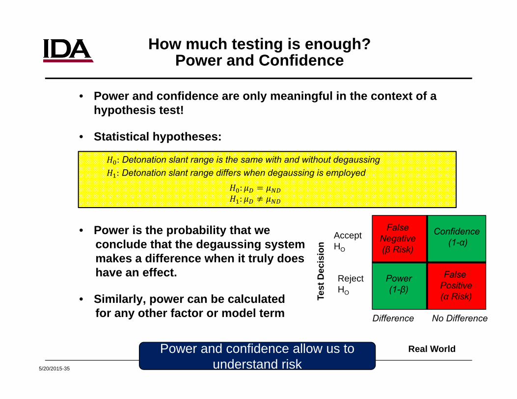
How much testing is enough?Power and Confidence

• Power and confidence are only meaningful in the context of a hypothesis test!

• Statistical hypotheses:

• Power is the probability that weconclude that the degaussing systemmakes a difference when it truly doeshave an effect.

• Similarly, power can be calculated for any other factor or model term

Power and confidence allow us to understand risk

No Difference

Real World

Accept HO

Reject HO

Confidence(1-α)

Power (1-β)

Difference

False Positive(α Risk)

False Negative(β Risk)

Test

Dec

isio

n

: Detonation slant range is the same with and without degaussing: Detonation slant range differs when degaussing is employed

::

5/20/2015-36

Test Design Comparison: Statistical Power

• Compared several statistical designs – Recommended a replicated central composite design with 28 runs– Power calculations are for effects of one standard deviation at the

90% confidence level


1 Full Factorial (2-level) 8

2 Full Factorial (2-level) replicated 16

3 General Factorial (3x3x2) 18

4 Central Composite Design 18

5 Central Composite Design (replicated center point) 20

6Central composite Design with replicated factorial points (Large CCD)

28

7 Replicated General Factorial 36

Statistical power provides an objective measure of how much testing is enough

5/20/2015-37

The Relationship between Power and Prediction

• In operational testing, we are often most concerned with post test predictions and the width of our interval estimates

• Power provides a strong indication of how wide the confidence intervals when reporting results

Scaled

by σ

Several three factor designs illustration the

link between power and confidence interval

width

5/20/2015-38

A Final Caution:Factor Power vs. One Sample Power

• If characterization is the goal, then avoid one-sample hypothesis tests on average performance, they can be highly misleading

• Stryker Mobile Gun System hypothetical test designs

Mission Attack DefendIllum OPFOR Terrain Urban Mixed Forest Desert Urban Mixed Forest DesertDay Low 1 1 1 1 1 1 1 1Day Med 1 1 1 1 1 1 1 1Day High 1 1 1 1 1 1 1 1Night Low 1 1 1 1 1 1 1 1Night Med 1 1 1 1 1 1 1 1Night High 1 1 1 1 1 1 1 1

Mission Attack DefendIllum OPFOR Terrain Urban Mixed Forest Desert Urban Mixed Forest DesertDay Low 8Day Med 8Day High 8Night Low 8Night Med 4 4Night High 4 4

vs

One Sample Power99.5%

Factor PowerIllum 98.4%OPFOR 88.7%Terrain 75.3%Type 98.4%

One Sample Power99.5%

Factor PowerIllum 95.8%OPFOR 47.5%Terrain 41.3%Type N/A

5/20/2015-39

Collinearity/Correlation Coefficients

• Two or more factors are consider collinear if they move together linearly (as one increases, so does the other)

• A well designed experiment minimizes the amount of collinearity between factors

• Ideally, operational tests should be designed to support at least all main effects and two way interactions.

– When there are a large number of factors, it is often not possible to design operational tests to this standard

• Correlation plots allow us to understand the tradeoffs in modeling

Collinearity between factors decreases the power of a DOE and increases CI width

5/20/2015-40

Correlation Coefficients - No Correlation

Time of Day

Target Speed

Target Type Update Rate Clutter

Day Fast Tracked 30 Y

Day Fast Wheeled 12 N

Day Fixed Tracked 12 N

Day Fixed Wheeled 30 N

Day Slow Tracked 12 Y

Day Slow Wheeled 30 Y

Night Fast Tracked 30 N

Night Fast Wheeled 12 Y

Night Fixed Tracked 30 Y

Night Fixed Wheeled 12 Y

Night Slow Tracked 12 N

Night Slow Wheeled 30 N

• Small Diameter Bomb II Normal Attack Example

– 12 Run Main Effects Only Design

• Even though this design is not a full factorial the main effects are all uncorrelated

– Blue is perfectly uncorrelated– Red is perfectly (100%) correlated

5/20/2015-41

Correlation Coefficients – 100% Correlation

Time of Day

Target Speed


Day Fast Wheeled 30 Y






Night Fast Tracked 30 N

Night Fast Tracked 12 Y







• Target type is perfectly correlated with time of day!

– Blue is perfectly uncorrelated– Red is perfectly (100%) correlated

5/20/2015-42

Correlation Coefficients – Some Correlation

Time of Day

Target Speed


Day Fast Wheeled 30 Y


Day Fixed Tracked 12 N


Day Slow Tracked 12 Y


Night Fast Wheeled 30 N

Night Fast Wheeled 12 Y


Night Fixed Wheeled 12 Y


Night Slow Wheeled 30 N



• Practical constraints can introduce acceptable correlations

– e.g., Only wheeled vehicles can move fast

5/20/2015-43

Model Supported and Correlation

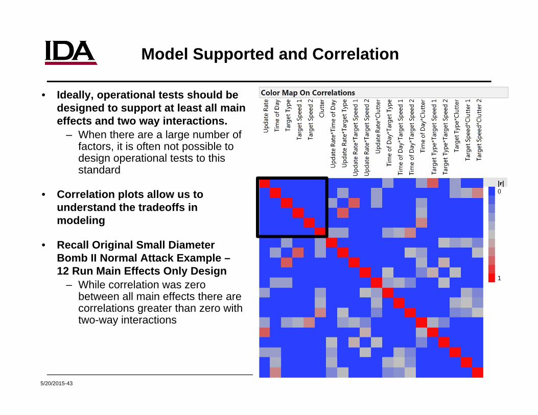
• Ideally, operational tests should be designed to support at least all main effects and two way interactions.

– When there are a large number of factors, it is often not possible to design operational tests to this standard

• Correlation plots allow us to understand the tradeoffs in modeling

• Recall Original Small Diameter Bomb II Normal Attack Example –12 Run Main Effects Only Design

– While correlation was zero between all main effects there are correlations greater than zero with two-way interactions

5/20/2015-44

TEMP and Test Plan Review:Design Evaluation

1. Overall Design Approach– Is the test size proposed in the experimental design reasonable? Is it

consistent with the resources section?– Are all the important factors included within the design?

2. Model Supported– Does the model supported at least a two-factor interaction model?

» If not, are the most important two-factor interactions estimable?– Are quadratic effects (or at least center points) included for

continuous factors?3. Power

– Is power calculated for the primary response variables?– Is there high power for main effects?

» Note, there is no DOT&E rule for what constitutes “high power” » Power calculations should always be based on expected effect size and

estimated variance.» However, in cases where no estimate is possible, historical data analysis

have shown us that good rules of thumb are:• Confidence level = 95%, signal to noise ratio = 2• Confidence level = 80%, signal to noise ratio = 1• These guidelines should only be used as a first “sanity check”

5/20/2015-45

TEMP and Test Plan Review:Design Evaluation

3. Power– What is the power for interaction and higher order term effects?

» It is often reasonable to accept lower power for these terms– What is the sensitivity of the power to the final analysis model?

» That is, if none of the interaction effects are significant, how does the power change for main effects?

– Note: power calculations should only need to be provided for the few primary response variables identified for the test, not every measure in the TEMP/Test Plan

» If the one primary response variable is pass/fail (binary) and another is continuous, separate power calculations should be provided

4. Correlation– Is there low correlation (< 0.5) between all anticipated model terms?– If not, why is the correlation structure acceptable?

5/20/2015-46

Design CoverageN

umbe

r of F

acto

rs

Classical Factorials

Fractional FactorialDesigns

Response Surface Method Designs

OptimalDesigns

Combinatorial Designs

Software Testing/ Deterministic Processes

5/20/2015-47

Common Design Mistakes

• Failure to link goals, responses, factors, levels, and resourcing– All elements may be present but there also needs to be a linkage

• Failure to link analysis to the design– Roll-up power calculations versus power calculations by factor– Power should always be reported for at least all main effects!

• Elimination of factors or factors left uncontrolled, because “we can’t afford that many factors in a design”

– Sparsity of effects– Fractional factorials, small response surface designs, and optimal

designs can support a large number of factors.

• Trying to build one design for the full operational test

5/20/2015-48

Key Takeaways: Experimental Design

• There are many types of experimental designs– Design choice depends on test objectives, number of factors/levels,

and risk tolerance

• Test designs should support characterization– Characterization implies that we are interested in predictions

across the design space– This typically requires designing for models that contain at least

main effects and most two-factor interactions– Higher order terms improve predictions

• Power is a useful metric for assessing test adequacy and selecting an appropriate design

– Other measures exist, correlation structures are useful tools for explaining test designs.

– Roll-up power calculations are misleading and inappropriate for assessing designed experiments

5/20/2015-49

Backup Material

5/20/2015-50

Power versus Confidence Interval Half Widthfor various factorial experiments

5/20/2015-51

Common DOE Methods for Software

• Factor Covering or Combinatorial Designs– How to test as quickly as possible when the test space is large and

made up of combinations of selections

• Space Filling– How to spread out test cases evenly when the test space is large and

continuous– For example,

• Both methods improve the chance of finding defects that are ‘combinatorial’ or ‘regional’

5/20/2015-52

Software Test Design: Risk in Test

• Outcomes may change for one set of inputs, the change is ‘diffused’ across the levels of the input factors

• The RISK: Data is confusing or not representative due to random chance

• Outcomes may change little for one set of inputs, but may change unpredictably if the inputs are changed

• The RISK: Defects go undetected thanks to incomplete or inefficient coverage of the space

• Traditional Textbooks of DOE focuses on statistical risk (probabilistic)• Modern DOE includes design-methods for software, where non-

statistical risks can be a primary (or even the only) focus

Statistical-Risk Non-Statistical-Risk

In software testing the goal is to cover as much of the space as possible, this is done at the expense of being able to determine

cause and effect relationships!

5/20/2015-53


• Combinatorial Test Designs are tests that cover a large number of combinations of factors extremely quickly, searching for problems

– Trade-off: we lose the ability to determine cause and effect, therefore process must be deterministic

– Examples: bugs in software, link inoperability

• Everyday example: How many tests? There are 10 effects, each can be

on or off All combinations equals 210 = 1,024

tests What if our budget is too limited for

these tests? Main effects are easy – 10

tests But what about interactions?

90 two-way interactions 120 three-way

interactions

5/20/2015-54


• How can we cover all 120 three-way interactions?

Since we can pack 3 triples into each test, we need no more than 40 tests.

Each test exercises many triples:

0 1 1 0 0 0 0 1 1 0

• Each row is several simultaneous tests

• Finding combinatorial designs is difficult a process.

• Requires computer software• NIST• Hexawise• JMP 12 Pro

5/20/2015-55

Factor Covering

Box 1 Box 2 Box 3 Box 4 Box 5 Box 6 Box 7 Box 8 Box 9 Box 101 1 1 1 1 1 1 1 1 11 1 1 1 0 0 0 0 0 01 0 0 0 1 1 1 0 0 00 1 0 0 1 0 0 1 1 00 0 1 0 0 1 0 1 0 10 0 0 1 0 0 1 0 1 1

It takes FIVE cases to cover all pairs for FOUR factors (2 levels)

We can extend into TEN dimensions with only ONE more case…

5/20/2015-56

Space Filling

• Space Filling is an efficient way to search or cover continuous input spaces

• Space Filling algorithms spread out test points using tailored optimality criteria

• 3 popular algorithms:– Sphere-Packing

» Maximize the smallest distance between neighbors

» Effect: Moves points out to boundaries– Uniform

» Minimize discrepancy from a uniform distribution

» Effect: Spreads points within interior– Latin Hypercube

» Assign n congruent levels and minimize covariance

» Effect: Combination of the above

5/20/2015-57

Summary of DOE for Software

• There is a science to software system test

• The appropriateness of designs depends on if outcomes are deterministic vice probabilistic

• There ARE tools and techniques (we covered some) that have utility for software-intensive test design:

– Factor Covering for covering sub-configurations (categorical factors)– Space Filling for spanning regions (continuous factors)

3 experimental designs

Documents