2d fem analysis compared with the in-situ deformation … · 2019-10-31 · 10 plaxis bulletin l...

10 Plaxis Bulletin l Autumn issue 2015 l www.plaxis.com

2D FEM analysis compared with the in-situ deformation measurements: A small study on the performance of the HS and HSsmall model in a design

The deformation behaviour as a result of excava-tion of a building pit in the inner city of Amsterdam is studied using the small strain stiffness model in PLAXIS 2D. The numerical results of deformations on the sheet pile wall during the different excavation stages obtained using PLAXIS are compared with the measured data. The objective of this study is to investigate the differences in computed deformation of the sheetpile wall when using the Hardening Soil model (HS) and the Hardening Soil Small Strain Stiff-ness model (HSsmall) employing the correlations of Alpan (1970) and Benz & Vermeer (2007) compared with the inclinometer data to asses their performance in an actual design process.

Background on the Small Strain Stiffness modelIt has been discovered from dynamic response analysis (Seed & Idriss, 1970), that most soils exhibit curvilinear stress-strain relationships. The shear modulus G (see Figure 1) is usually expressed as the secant modulus found at the extreme points of the hysteresis loop. The damping factor is proportional to the area found inside the hysteresis loop. The applied terminology of damping usually means the dissipation of strain energy during cyclic loading. From the defi nition of both physical properties, it shows that each of them will depend on the magnitude of the strain for which the hysteresis loop is determined. Thereby, both the shear moduli and damping factors must be determined as functions of the induced strain in a soil. Several studies have shown that the shear moduli of most soils decay monotonically with strain. Cavallaro et al. (1999), Mayne & Schneider (2001), and Benz et al. (2009) suggest that when the maxima are at very small strain levels, i.e. less than 10-6 to 10-5, which is associated to recoverable, the material behaviour is almost purely elastic (see Figure 2).

Ir. Martin A. op de Kelder, CRUX Engineering bv

Small-strain stiffness is seen as a fundamental property that almost all soils ranging from colloids to gravels and even rocks exhibit.

This is the case for static and dynamic loading, and for drained and undrained conditions. In literature, small-strain stiffness is

assumed to exist due to inter-particle forces within the soil skeleton. Therefore, it can be altered only if these inter-particle forces

are rearranged (Benz et al., 2009).

Figure 1: a) Defi nition of the secant shear stiffness Gsec of the hysteresis loop, b) Decrease of Gsec from its maximum value Gmax with increasing shear strain amplitude γampl [after Wichtmann & Triantafyllidis (2009)]

Figure 2: Characteristic stiffness-strain behaviour in logarithmic scale [after Atkinson & Sallfors (1991) and Mair (1993)]

www.plaxis.com l Autumn issue 2015 l Plaxis Bulletin 11

2D FEM analysis compared with the in-situ deformation measurements: A small study on the performance of the HS and HSsmall model in a design

The difference between ‘small’ strains and ‘large’ strains is usually taken at the point where classical laboratory testing, such as triaxial or oedometer testing without special instrumentation like local strain gauges has reached its limits, i.e. around 10-3 or 0.1%.

The preferred approach for the establishment of small strain stiffness parameters, which can be used in routine design obviously, starts with laboratory testing. The small strain stiffness implementation in PLAXIS is based on the small strain overlay model (Benz et al., 2009). Parameters G0 and γ0.7 are required input parameters. At the absence of experimental data for the determination of these two required parameters, approximations through correlations can be appropriate.

One of the often used correlations is the one sug-gested by Alpan (1970), where he used a single curve that describes the relationship between ‘static’ and ‘dynamic’ Young’s moduli. However, in his paper it does not become exactly clear what he means with the ‘static’ modulus as controversially discussed in literature by Benz & Vermeer (2007) and Wichtmann & Triantafyllidis (2007, 2009). Alpan (1970) reported the tangent elastic modulus E i as the inclination of the nearly linear initial portion of the deviatoric stress – strain curve, implying a stiffness for the fi rst loading, like today we would use E50. Wichtmann & Triantafyllidis (2009) further add to this that un- and reload cycles are not discussed in the paper of Alpan (1970) although Benz & Vermeer (2007) argued for Eur. Benz (2007) further adds that Alpan’s Estat is the apparent elastic Young’s modulus in conventional soil testing, e.g. (εa ≈ 10-3) in triaxial testing. According to Benz (2007) for soils with known Young’s modulus in triaxial unloading-reloading, the Alpan (1970) chart can provide an estimate for its very small-strain modulus E0.

In Deutsche Gesellschaft für Geotechnik (DGGT) (2001), the correlation between dynamic and static stiffness modulli is given in terms of the modulus M for one-dimensional compression (zero lateral strain). The correlation has been derived from the curve of Alpan (1970), but in contrast to that curve, DGGT (2001)

provides upper and lower boundaries for different types of soils. Unfortunately, no testing procedure for the determination of Mstat is prescribed, however because no un- and reloading cycles are mentioned in that research, the input parameter Mstat is probably meant as the stiffness modulus during fi rst loading. According to Wichtmann & Triantafyllidis (2009), the chart is used in this way in practice. Benz & Vermeer (2007) provided an alternative correlation between Mdyn/Mstat and Mstat, which is also based on the curve of Alpan (1970). In 2009, Wichtmann & Triantafyllidis have reported that for a given value of Mstat, the ratio of Mdyn/Mstat predicted by the correlation of Benz & Vermeer (2007) lay signifi cantly higher than those obtained from the relationship recommended in DGGT (2001).

They suggested that this is probably due to a different interpretation of Alpan’s Estat. Furthermore, Wichtmann & Triantafyllidis (2009) tested four samples of sand with different grain size distributions. If Estat is approximated by Estat = Eur ≈ 3E50 (Benz & Vermeer, 2007), instead of Estat ≈ E50 (Alpan, 1970), the obtained results can give a good fi t for sands. The curve of Alpan (1970) underestimates in the same experiment the obtained values Edyn/E50 by a factor in the range between 1,5 and 2,5. Both Benz & Vermeer (2007) and Wichtmann & Triantafyllidis (2009) concluded that if the original correlation by Alpan (1970) can be interpreted as Estat = Eur ≈ 3E50, based on both authors experiences, Alpan’s chart would provide reasonable estimates for the stiffness of soils.

Figure 3: Comparison of the correlations between Edyn/Estat and Estat according to Alpan (1970), DGGT (2001) and by Benz & Vermeer (2007) [after Wichtmann & Triantafyllidis (2009)]


As shown in Figure 3 and based on the aforemen-tioned statements, the following can be summarized in regard to the interpretation of Alpan’s Estat:

• Alpan (1970) Estat = Eur ≈ 3 E50

• DGGT (2001) Estat = Eur ≈ 3 E50

• Benz & Vermeer (2007) Estat = Eur ≈ 3 E50

Once Estat or Mstat has been determined, which is the static Young’s modulus E or the one-dimensional compression modulus M at very small strains in essence of E0 and M0 respectively, the small strain shear modulus G0 can be calculated if the Poisson ratio ν is known, or an estimation of it can be used.

The following relationship (Eq. 1) can be used to estimate the initial shear modulus G0 (Wichtmann & Triantafyllidis, 2009):

where:E0 = the Young’s modulus at very small strains [MPa]

ν = Poisson’s ratio [-]

For the calculation of the threshold shear strain γ0.7 at which the normalized small strain shear modulus G/G0 has reduced to 70%, the following relationship (Eq. 2) is used (Hardin & Drnevich, 1972):

where:c' = drained cohesion [kN/m2]

φ' = drained angle of internal friction [deg]

k0 = neutral earth pressure coefficient [-]

σ1' = effective vertical stress

(usually equal to σ3' = 100 kPa) [kN/m2]

Case Study - Vijzelhof ProjectThe Vijzelhof project in Amsterdam consists of a single storey underground parking space, which will be realised by the construction of a building pit using sheet piles and a single strut layer. Considering the non-linear behaviour of soils, a higher order constitutive model to capture most of the actual soil behaviour is needed. Herein, the deformation behaviour and its impact on the surrounding buildings will be analysed using the FEM code PLAXIS 2D. Measurements were carried out by the in-situ monitoring. In view of validation, the numerical results of horizontal deformations will be compared with the measured data. In order to capture the deformation behaviour of the sheet piles, several inclinometers were installed at the project site. The corresponding soil profile is presented in Figure 4. In this paper, the study is concentrated on the cross-section 1-1 because this was the most critical area. An overview of where the buidling pit is constructed can be seen in Figure 5.

Results and DiscussionsTo assess the deformations as a result of excavation, two phased calculations were performed. For both calculation phases, the predicted deformations of the left sheetpile will be compared with the measured data obtained during the construction of the building pit. The objective of this study is to investigate the performance of the HS model and HSsmall model employing the correlations of Alpan (1970) and Benz & Vermeer (2007), and to compare the numerical results with the inclinometer data so as to asses the model performance during the design process.

( ) ( )0 0 01 1 2

2 1 2 1G E M ν

ν ν− ⋅

= ⋅ = ⋅⋅ + ⋅ −

( )( ) ( ) ( ){ }' ' ' '0.7 1 0

0

1 2 1 2 1 29

c cos K sinG

γ ϕ σ ϕ≈ ⋅ ⋅ ⋅ + ⋅ + ⋅ + ⋅ ⋅⋅

Figure 4: Geotechnical soil profiles based on CPT’s and borings (op de Kelder, 2013)

( ) ( )0 0 01 1 2

2 1 2 1G E M ν

ν ν−

= =+ − (1)

(2)( ) ( )'0.7 1 0

0

1 2 ' 1 cos 2 ' 1 sin 2 '9

c kG

γ ϕ σ ϕ ≈ + + +

2D FEM analysis compared with in-situ deformation measurements: A small study on the performance of the HS and HSsmall model in a design


2D FEM analysis compared with in-situ deformation measurements:A small study on the performance of the HS and HSsmall model in a design

Figure 5: Study area [CRUX (2011), op de Kelder (2013)]

Figure 6: Global dimensions of the FEM model (top), zoomed in view (bottom)


It has to be noted that in any nummerical model, the presented results are not only affected by the selected small-strain stiffness parameters and used correlations but also by the other soil parameters, modelling assumptions, applied boundary conditions, phasing, etc. Keeping that in mind, in this article, the first and the last excavation phase will be discussed.

Phase 1The first excavation phase covers the modelling of excavation of the soils to a level of NAP +0.00m and of those that slope to NAP -0.50m (Figure 7). Figure 8 shows the predicted and measured horizontal displacements of the sheet pile. It can be seen that there is a large difference in deformations between the HS and HSsmall model. When compared to the

Figure 7: Configuration of phase 1

measured data, the HSsmall model underestimates the sheet pile horizontal deformation at the upper part of the sheet pile, whilst the HS model overestimates the horizontal deformation almost over the entire length of the sheet pile. The HS model in particular shows a good agreement with the measured data around the upper part of the pile. Clearly, the discrepancy between the numerical results obtained using the HS model and the field measurements is due to the inability of the HS model to incorporate small-strain stiffness behaviour.

Comparing the HSsmall model with the measured data, the numerical results at top level of the sheet-pile are approximately three times lower than the measured data. This is due to the very stiff response

of the soil in the first excavation phase as strains are still in the very small strain domain, thus a very stiff response results in small deformations. As the depth increases, the deformation decreases. Consequently, the soil response is stiffer at greater depth due to its stress-dependent stiffness moduli, and the relative numerical deformation difference between the HS model and HSsmall model becomes relatively small.

For the calculation of HSsmall parameters several correlations are available. For the calculation of the shear modulus G0, the correlation of Benz & Vermeer (2007) and that of Alpan (1970) interpreted according to Benz & Vermeer (2007), i.e. Estat ≈ Eur ≈ 3E50 was used. The threshold shear strain γ0.7 is calculated using Eq. (2).

Alpan (1970) Benz & Vermeer (2007)

Layer nameγunsat γsat c' ϕ’ νur k0 E50

ref Eoedref Eur

ref m G0 γ0.7 G0 γ0.7

[kN/m3] [kN/m3] [kPa] [deg] [-] [-] [kPa] [kPa] [kPa] [-] [kPa] [-] [kPa] [-]

Sand (anthropogenic) 15 18,4 0,1 30 0,15 0,50 2,00E+04 2,00E+04 6,00E+04 0,80 9,31E+04 1,55E-04 2,13E+05 6,78E-05

Estuary clay 16,9 16,9 6 26 0,15 0,50 1,00E+04 4,00E+03 2,50E+04 0,80 5,57E+04 2,74E-04 1,22E+05 1,25E-04

Holland peat 10,5 10,5 5 20 0,15 0,65 2,00E+03 1,00E+03 1,00E+04 0,80 3,39E+04 4,05E-04 7,18E+04 1,91E-04

Old marine clay 16,5 16,5 7 33 0,15 0,50 9,00E+03 4,30E+03 2,50E+04 0,80 5,57E+04 3,13E-04 1,22E+05 1,42E-04

Mudflat deposits sand 17,9 17,9 2 35 0,20 0,40 1,20E+04 5,00E+03 3,30E+04 0,56 6,26E+04 2,43E-04 1,39E+05 1,09E-04

Mudflat deposits clay 15,2 15,2 8 34 0,15 0,58 9,00E+03 6,10E+03 1,80E+04 0,80 4,63E+04 4,04E-04 1,01E+05 1,86E-04

Base peat 11,7 11,7 6 21 0,15 0,65 2,00E+03 1,00E+03 1,00E+04 0,80 3,39E+04 4,30E-04 7,18E+04 2,03E-04

1st sand layer 19,8 19,8 0,1 33 0,20 0,40 4,00E+04 3,00E+04 2,00E+05 0,50 1,92E+05 7,40E-05 4,62E+05 3,08E-05

Alleröd, clay 18,5 18,5 3 33 0,20 0,40 1,70E+04 1,30E+04 4,50E+04 0,50 7,51E+04 2,02E-04 1,69E+05 8,96E-05

2nd sand layer 19 19 0,1 35 0,20 0,40 3,50E+04 3,50E+04 1,90E+05 0,50 1,85E+05 7,88E-05 4,47E+05 3,27E-05

Table 1: Soil properties



Figure 8: First excavation phase

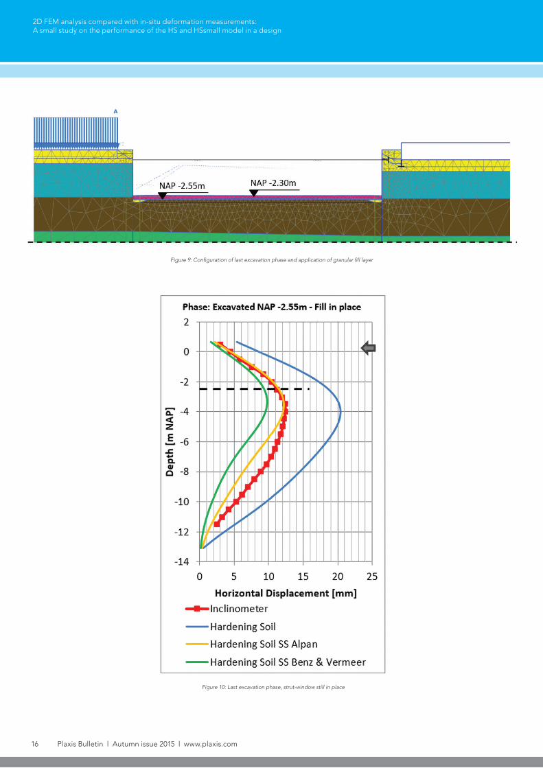
Phase 2The last excavation phase focusses on the deformation behaviour as a result of the excavation to NAP -2.55 m and fi nishing off the granular fi ll layer (top level NAP -2.30 m) as shown in Figure 9. The black dotted line in Figure 9 roughly indicates the surface level inside the building pit, in which the arrow represents the strut level.

The predicted horizontal deformations are presented in Figure 10. It can be sen that the numerical results obtained using the HSsmall model are in good agreement when compared to the measured data. Particularly in the lower part of the pile, the predicted deformations obtained using the HSsmall model underestimate the actual deformations.

This is likely caused by the relative high small-strain stiffness behaviour in the cohesive soil layers. In con-trast, the HS model overestimates the deformations of the sheet pile due to its inabbility to capture the actual small-strain behaviour in the soil troughout the excavation phasing.

The relative difference of deformations at the middle section of the sheet pile decreases as the excavation level increases. The deformations when obtained using the HSsmall model for both correlations are roughly two times lower than those of the HS model. The small-strain stiffness behaviour at this depth suggests that the G/Gur ratio in the mudfl at deposits layer containing sand is between 3 and 4. In the mudfl at deposits layer containing clay it is between 4 and 5.

In the base peat layer it is between 5 and 6. Compared to earlier phases (which are not all discussed in this article), the response of the soil is stiffer meaning that there is an increase in small-strain behaviour.

The stiffer response of the soil is probably triggered by the fact that the granular fi ll results in a ‘load trans-versal’ (after unloading from the excavation sequence the soil is compressed again), which causes a part of the elastic straining to be recovered in the HSsmall model and higher stiffness of the soil is observed.

The ordinary HS model has a lack of the ability to take into account this kind of small strain soil behaviour and therefore does not produce similar numerical results.



Figure 9: Confi guration of last excavation phase and application of granular fi ll layer

Figure 10: Last excavation phase, strut-window still in place



Conclusions Acknowledging that in any numerical model, the presented results are not only affected by the se-lected small-strain stiffness parameters and used correlations but also by the other soil parameters, modelling assumptions, applied boundary conditions, phasing, etc. the following conclusions can be drawn.

By means of the FEM code PLAXIS 2D the deforma-tion behaviour as a result of excavation of a building pit in the inner city of Amsterdam was investigated. Two different constitutive models, namely the HS model and HSsmall model were used in the analysis. Furthermore, the HSsmall model was distinguished based on either the Benz & Vermeer (2007) or Alpan (1970) correlations. To validate the model, the numeri-cal results are compared with the measured data.

When compared to the measured data, this study suggests that the HSsmall model employing either the Benz & Vermeer (2007) correlation or the Alpan (1970) correlation are better in capturing the soil behaviour than employing the HS model. When using the aformentioned correlations Estat should be interpreted as Estat = Eur ≈ 3E50. Then, the small strain stiffness behaviour which soils do exibit can be included in the numerical computation by employ-ing the HSsmall model. The Alpan (1970) correlation provides lower small strain stiffness moduli G0 and thus will be more conservative when applied in design compared to Benz & Vermeer (2007).

Secondly, this study also suggests that the HSsmall model, when using the presented correlations of Alpan (1970) and Benz & Vermeer (2007) in combination with the presented parameterset, tends to overestimate small-strain stif fness behaviour in the cohesive layers. Relatively high G/Gur ratios were computed in the cohesive layers compared to the non-cohesive layers that can result in smaller deformations. This may be related to the fact that the small-strain stiffness correlations of Alpan (1970) and Benz & Vermeer (2007) used in this study, are established

based on primarily tests of non-cohesive materials like sands and gravels. Only a small amount of tests have so far been conducted on cohesive materials like clays and peats.

The correlations provided by Alpan (1970) or Benz & Vermeer (2007) in combination with the unload-reload stiffness Eur and other soil properties such as c, φ, k0 and ν, can be used to determine the actual small-strain stiffness parameters G0, γ0.7 used in the HSsmall model of PLAXIS. At the absence of experi-mental data for the determination of parameters G0 and γ0.7, approximations through correlations can be appropriate. Keeping in mind that the standard procedure for estimating Eur through correlations in PLAXIS is to use Eur equals to 3E50.

References• Alpan, I. (1970). The geotechnical properties of soils.

Earth-Science Reviews, Vol. 6, pp 5–49.• Atkinson, J.H., Sallfors, G. (1991). Experimental

determination of soil properties. Proceedings of the 10th ECSMFE, Vol. 3, Florence, pp 915-956.

• Benz, T. (2007). Small-strain stiffness of soils and its numerical consequences. PhD Thesis, Dissertationsschrift. Mitteilung 55 des Instituts für Geotechnik, Universität Stuttgart.

• Benz, T., Vermeer, P.A. (2007). Zuschrift zum Beitrag ”Über die Korrelation der ödometrischen und der ”dynamischen” Steifigkeit nichtbindiger Böden” von T. Wichtmann und Th. Triantafyllidis (Bautechnik 83, No. 7, 2006). Bautechnik, Vol. 84 (5), pp 361–364.

• Benz, T., Vermeer, P.A., Schwab, R. (2009). A small-strain overlay model. International Journal for Numerical and Analytical Methods in Geomechanics, Vol. 33, pp 25–44.

• Benz, T., Vermeer, P.A., Schwab, R. (2009). Small-strain stiffness in geotechnical analyses. Bautechnik, Vol. 86 (S1), pp 16-27.

• Cavallaro, A., Maugeri, M., Lo Presti, D.C.F., Pallara, O. (1999). Characterising shear modulus and damping from in situ and laboratory tests for the seismic area of Catania, Proceedings of

the 2nd International Symposium on Pre-Failure Deformation Characteristics of Geomaterials, Torino 27-30 September, Balkema, Vol. 1, pp 51-58.

• CRUX Engineering B.V. (2011). “Parkeergarage 'De Vijzelhof' Noorderstraat Amsterdam, Risicoanalyse omgevingsbeïnvloeding”, RA11249a2, pp 5 – 8.

• DGGT (2001). Empfehlungen des Arbeitskreises 1.4 ”Baugrunddynamik” der Deutschen Gesellschaft für Geotechnik e.V.

• Hardin, B.O., Drnevich, V.P. (1972). Shear modulus and damping in soils: design equations and curves. Journal of the Soil Mechanics and Foundations Division, Vol. 98 (SM7), pp 667–692.

• op de Kelder, M.A. (2013). 2D Finite Element Analysis of a building pit compared with in-situ measurements, M.Sc. Thesis, Faculty of Civil Engineering and Geosciences, Department of Geo-Engineering, Delft University of Technology

• Mair, R.J. (1993). Developments in geotechnical engineering research: application to tunnels and deep excavations. Proceedings of Institution of Civil Engineers, Civil Engineering, pp 27-41.

• Mayne, P.W., Schneider, J.A. (2001). Evaluating axial drilled shaft response by seismic cone. Foundations & Ground Improvement, GSP 113, ASCE, Reston/VA, pp 665-669.

• Seed H.B., Idriss, I.M. (1970). Soil moduli and damping factors for dynamic response analysis. Report 70-10, EERC, Berkeley, CA, U.S.A.

• Wichtmann, T., Triantafyllidis, T. (2007). Erwiderung der Zuschrift von T. Benz und P.A. Vermeer zum Beitrag ”Über die Korrelation der ödometrischen und der ”dynamischen” Steifigkeit nichtbindiger Böden” (Bautechnik 83, No. 7, 2006). Bautechnik, Vol. 84 (5), pp 364–366.

• Wichtmann, T., Triantafyllidis, T. (2009). On the correlation of ''static'' and ''dynamic'' stiffness moduli of non-cohesive soils. Bautechnik, Vol. 86 (S1), pp 28-39.


2d fem analysis compared with the in-situ deformation … · 2019-10-31 · 10 plaxis bulletin l...

Documents