2.882 system design and analysis - mit opencourseware · taesik lee © 2004 review design domain...
TRANSCRIPT

Taesik Lee © 2004
2.882 System Design and Analysis
February 14

Taesik Lee © 2004
What we’ll do today
• Information content• Robustness

Taesik Lee © 2004
Review
• Design process / Domain• Functional Requirements• Design Parameters

Taesik Lee © 2004
Review
Design Domain
• How do you go about ‘design’?
What do we want to achieve?
Howdo we want to
achieve it?
What do customers
want?
Howdoes our
product/system satisfy it?
What are the solutions to
be generated?
Howdo we want to generate it?

Taesik Lee © 2004
Review
Functional Requirement (FR)
• Functional requirements (FRs) are a minimum set of independent requirements that completely characterize the functional needs of the artifact (product, software, organization, system, etc.) in the functional domain.
– Independently achievable, in principle.– “The determination of a good set of FRs …… requires skill, …,
and many iterations”

Taesik Lee © 2004
Review
What constitute a GOOD set of FRs?
• MECE: Mutually Exclusive and Collectively Exhaustive• One FR carries only one requirement
– Juxtaposing two requirements into one doesn’t make them a single requirement
• Solution neutral– “Cover the battery contact by a plastic sliding door”
• Clarity/specificity– Bad example: missing target range, time factor, etc.
• Logical hierarchical structure
Taesik Lee © 2004
Review
Design Parameter (DP)
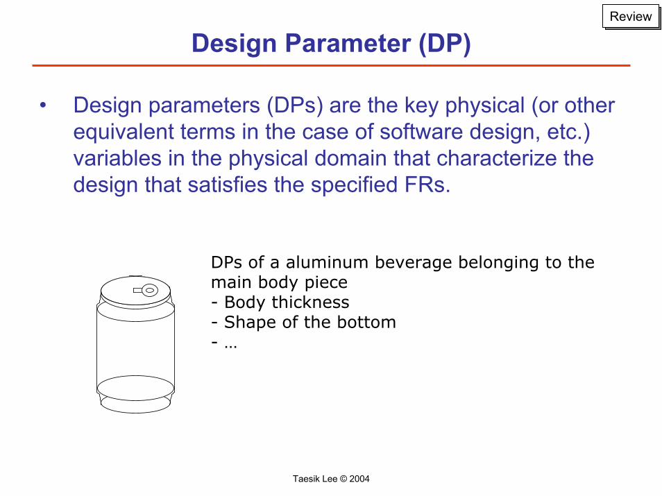
• Design parameters (DPs) are the key physical (or other equivalent terms in the case of software design, etc.) variables in the physical domain that characterize the design that satisfies the specified FRs.
DPs of a aluminum beverage belonging to the main body piece- Body thickness- Shape of the bottom- …

Taesik Lee © 2004
Review
Searching for a DP
• “Nothing substitutes for Knowledge”• Be open to wild idea
• Analogies– Benchmarking, Patents, Literatures, etc. in OTHER application
area • Visualization
– Sketch your idea• Stimuli
– Circulating ideas– Get exposed to foreign situations

Taesik Lee © 2004
Review
Design Hierarchy
• Decomposition by zigzagging– Process of developing detailed requirements and concepts by
moving between functional and physical domain– Yields a hierarchical FR-DP structure
FR1
FR11 FR12
FR111 FR112 FR121 FR122
FR1111 FR1112 FR1211 FR1212
DP1
DP11 DP12
DP111 DP112 DP121 DP122
DP1111 DP1112 DP1211 DP1212
: :

Taesik Lee © 2004
Review
• Decomposition– Process of breaking down a large problem into a set of smaller
ones so that each of the sub-problems is manageable• Zigzagging
– Decomposition process must involve both functional and physical domain by moving between the two domains
– Upper-level choice of DP drives the FRs at the next level• Lower-level FRs are a complete description of
functional needs of the upper-level FR-DP pair– Parent-Child relationship

Taesik Lee © 2004
InformationContentsInformation content
• Design range• System range• Probability of success• (Allowable) Tolerance
Taesik Lee © 2004
InformationContentsDesign Range
• Examples of “range” in FR statements- Maintain the speed of a vehicle at a designated mph in the
range of 0mph - 90mph- Maintain the speed of a vehicle at a x mph +/- 5mph- Ensure no leakage under pressure up to 100 bar- Ensure 99% successful ignition at the first attempt in the
temperature range of -30°C ~ 80°C- Generate nailing forces of up to 2,000 N

Taesik Lee © 2004
InformationContentsDesign Range
• Specification for FR• Acceptable range of values of a chosen FR metric; Goal-post• Different from “tolerance”• Different from “operating range”• Target value (nominal), Upper bound, Lower bound
FR FR- ∞ (or 0)∞x FR* y x xFR
Greater than x(Larger the better)
Smaller than x(Smaller the better)
Between x and y
Taesik Lee © 2004
InformationContentsSystem Range
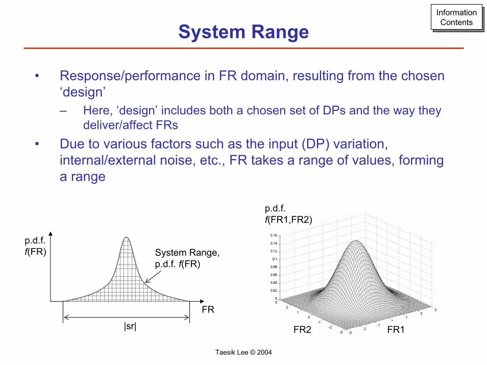
• Response/performance in FR domain, resulting from the chosen ‘design’– Here, ‘design’ includes both a chosen set of DPs and the way they
deliver/affect FRs• Due to various factors such as the input (DP) variation,
internal/external noise, etc., FR takes a range of values, forming a range
FR1FR2
p.d.f.f(FR1,FR2)
p.d.f.f(FR)
FR
System Range,p.d.f. f(FR)
|sr|

Taesik Lee © 2004
InformationContentsInformation content
∫=u
l
dr
dr
dFRFRfFRP )()(
∫−=−=−=u
l
dr
dr
dFRFRfFRPPI )(log)(loglog 222
FRdru
p.d.f.f(FR)
drl
System Range,p.d.f. f(FR)
Design Range
|sr|
Common Range, AC
|dr|
FRdru
p.d.f.f(FR)
drl
System Range at time t0,f(FR, t0)
Design Range |dr|
t
FRdru
p.d.f.f(FR)
drl
System Range at time t0,f(FR, t0)
Design Range |dr|
t
Where do we get f(FR)?

Taesik Lee © 2004
InformationContents
Information content for multiple FRs
nn pFRFRFRI ,...,2,12,,2,1 log)( −=L
∫=hyperspacedesign
2121,...,2,1 ),,,( nnn dFRdFRdFRFRFRFRfp LL
If Uncoupled,
n
drnnnn
drdr
dr dr drnnnn
ppp
dFRFRfdFRFRfdFRFRf
dFRdFRdFRFRFRFRfp
...
)()()(
...),...,,(
21
12
2221
111
1 22121,...,2,1
=
×××=
=
∫∫∫
∫ ∫ ∫L
L
)(...)()()( 21,,2,1 nn FRIFRIFRIFRFRFRI +++=L

Taesik Lee © 2004
InformationContents
If Decoupled,
n
dr dr drnnnnn
dr dr drnnnn
dFRdFRdFRFRfFRFRf
FRFRFRFRfFRFRFRFRf
dFRdFRdFRFRFRFRfp
... )()(
),...,,(),...,,(
...),...,,(
21112
1 22211121
1 22121,...,2,1
L
LL
L
∫ ∫ ∫
∫ ∫ ∫
−−−=
=
⎭⎬⎫
⎩⎨⎧
⎥⎦
⎤⎢⎣
⎡=
⎭⎬⎫
⎩⎨⎧
2
1
2
1
DPDP
cbOa
FRFR
∫ ∫
∫ ∫
∫ ∫
⎭⎬⎫
⎩⎨⎧
=
=
=
111
2212
1 221112
1 221212,1
)()(
)()(
),(
dr dr
dr dr
dr dr
dFRFRfdFRFRFRf
dFRdFRFRfFRFRf
dFRdFRFRFRfp
For example,
Taesik Lee © 2004
InformationContents
⎟⎠⎞
⎜⎝⎛ −=
⋅−=
12
122
1
1
FRabFR
c
DPcbFR
cDP
⎭⎬⎫
⎩⎨⎧
⎥⎦
⎤⎢⎣
⎡=
⎭⎬⎫
⎩⎨⎧
2
1
2
1
DPDP
cbOa
FRFR
⎟⎠⎞
⎜⎝⎛=aFRg
aFRf 1)(
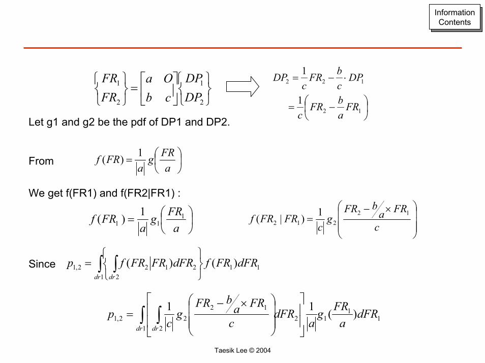
Let g1 and g2 be the pdf of DP1 and DP2.
From
We get f(FR1) and f(FR2|FR1) :
⎟⎟⎟
⎠
⎞
⎜⎜⎜
⎝
⎛ ×−=
c
FRabFR
gc
FRFRf12
2121)|(⎟
⎠⎞
⎜⎝⎛=aFRg
aFRf 1
111)(
∫ ∫⎭⎬⎫
⎩⎨⎧
=1
112
2122,1 )()(dr dr
dFRFRfdFRFRFRfpSince
11
11
22
1222,1 )(11 dFR
aFRg
adFR
c
FRabFR
gc
pdr dr∫ ∫ ⎥
⎥
⎦
⎤
⎢⎢
⎣
⎡
⎟⎟⎟
⎠
⎞
⎜⎜⎜
⎝
⎛ ×−=

Taesik Lee © 2004
InformationContents
Multiple FR system range
ExampleDesign range
FR1: [-0.5 , 0.5]FR2: [-2.0 , 2.0]⎭
⎬⎫
⎩⎨⎧
⎥⎦
⎤⎢⎣
⎡=
⎭⎬⎫
⎩⎨⎧
21
1101
21
DPDP
FRFR
DP1
DP2 FR2
FR1

Taesik Lee © 2004
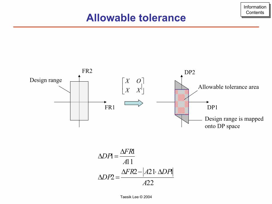
InformationContentsAllowable tolerance
• Defined for DP• Tolerances that DPs can take while FRs still remaining completely
inside design ranges• Unconditional tolerance• Conservative tolerancing
∆DP1 = ∆FR1A11
∆DP2 =∆FR2 − A21 ⋅ ∆DP1
A22
∆DP3 =∆FR3 − A31 ⋅ ∆DP1 − A32 ⋅ ∆DP2
A33
⎪⎭
⎪⎬
⎫
⎪⎩
⎪⎨
⎧
⎥⎥⎥
⎦
⎤
⎢⎢⎢
⎣
⎡=
⎪⎭
⎪⎬
⎫
⎪⎩
⎪⎨
⎧
321
333231022210011
321
DPDPDP
AAAAA
A
FRFRFR
Taesik Lee © 2004
InformationContentsAllowable tolerance
FR2 DP2Design range
⎥⎦
⎤⎢⎣
⎡XXOX
FR1 DP1
Allowable tolerance area
Design range is mapped onto DP space
221212
2
1111
ADPAFR
DP
AFRDP
∆⋅−∆=∆
∆=∆

Taesik Lee © 2004
InformationContents
Detecting change in system range
“Monitoring marginal probability of each FR is not only inaccurate but potentially misleading”
ExampleDesign range
FR1: [-0.5,0.5]FR2: [-2,2]⎭
⎬⎫
⎩⎨⎧
⎥⎦
⎤⎢⎣
⎡=
⎭⎬⎫
⎩⎨⎧
21
1101
21
DPDP
FRFR
Design parameter variation
Initial After changeDP1: [-1,1] DP1: [-1,1]DP2: [0,1.5] DP2: [-1,1.6]

Taesik Lee © 2004
p.d.fFR1
FR2
-1
-1 1
1.5
-1
0.5
FR2
FR1-1 1
0.5
0.5
(a) (b)
(c)
2
-2Design range
Joint p.d.f.(FR1,FR2)
2.5 2.5
1
p.d.fFR1
FR2
-1
-1 1
1.5
-1
0.5
FR2
FR1-1 1
0.5
0.5
(a) (b)
(c)
2
-2Design range
Joint p.d.f.(FR1,FR2)
2.5 2.5
1
p.d.fFR1
FR2
-1
-1 1
-1
0.3846
FR2
FR1
p.d.f
-1 1
0.5
0.6
(a) (b)
(c)
2
-2Design range
Joint p.d.f.(FR1,FR2)
2.6 2.6
.6
-2
p.d.fFR1
FR2
-1
-1 1
-1
0.3846
FR2
FR1
p.d.f
-1 1
0.5
0.6
(a) (b)
(c)
2
-2Design range
Joint p.d.f.(FR1,FR2)
2.6 2.6
.6
-2
Before DP2 change After DP2 change
DP1: [-1,1] DP2: [0,1.5]
DP1: [-1,1] DP2: [-1,1.6]
InformationContents
pFR1 pFR2 pFR1× pFR2 pFR1,FR2
Before 0.5 0.9583 0.4792 0.5
After 0.5 0.9654 0.4827 0.499
p.d.fp.d.f p.d.fp.d.f

Taesik Lee © 2004
InformationContentsSummary
• Joint probability unless it is uncoupled design• Assuming DPs are statistically independent, working in DP domain
is typically easier.
FR
D P
FR
D P
FR
D P
FR
D P
FR
D P
FR
D P
FR
D P
FR
D P
FR
D P
FR
D P
FR
D P
FR
D P
FR
D P
FR
D P
FR
D P
FR
D P
FR
D P
FR
D P
FR
D P
FR
D P
FR
D P
FR
D P
FR
D P
FR
D P
FR
D P
FR
D P
FR
D P
FR
D P
FR
D P
FR
D P
FR
D P
FR
D P
FR
D P
FR
D P
FR
D P
FR
D P
FR
D P
FR
D P
FR
D P
FR
D P
FR
D P
FR
D P
FR
D P
FR
D P
FR
D P
FR
D P
FR
D P
FR
D P
FR
D P
FR
D P
FR
D P
FR
D P
FR
D P
FR
D P
FR
D P
FR
D P
FR
D P
FR
D P
FR
D P
FR
D P
FR
D P
FR
D P
FR
D P
FR
D P
FR
D P
FR
D P
FR
D P
FR
D P
FR
D P
FR
D P
FR
D P
FR
D P
FR
D P
FR
D P
FR
D P
FR
D P
FR
D P
FR
D P
FR
D P
FR
D P
FR
D P
FR
D P
FR
D P
FR
D P
FR
D P
FR
D P
FR
D P
FR
D P
FR
D P
FR
D P
FR
D P
FR
D P
FR
D P
FR
D P
FR
D P
FR
D P
FR
D P
FR
D P
FR
D P
FR
D P
FR
D P
FR
D P
FR
D P
FR
D P
FR
D P
FR
D P
FR
D P
FR
D P
FR
D P
FR
D P
FR
D P
FR
D P
FR
D P
FR
D P
FR
D P
FR
D P
FR
D P
FR
D P
FR
D P
FR
D P
FR
D P

Taesik Lee © 2004
InformationContents“Information”
• In AD information content, by imposing design range, FR is transformed into a binary random variable.
ui= 1 (success) with P(FRi = success) 0 (failure) 1-P(FRi = success)
|dr|
FRdru
p.d.f.f(FR)
drl
System Range,p.d.f. f(FR)
Design Range
|sr|
Common Range,AC
I(ui= 1) ≡ - log2P(FRi =success)
I ( p )
0
1
2
3
4
5
6
7
0 0.2 0.4 0.6 0.8 1
P (FR =success)
I(p
) [bi
t]
H (P )
00.10.20.30.40.50.60.70.80.9
1
0 0.2 0.4 0.6 0.8 1
P (FR=success)
H(p
) [bi
t]
(a) (b)
I ( p )
0
1
2
3
4
5
6
7
0 0.2 0.4 0.6 0.8 1
P (FR =success)
I(p
) [bi
t]
H (P )
00.10.20.30.40.50.60.70.80.9
1
0 0.2 0.4 0.6 0.8 1
P (FR=success)
H(p
) [bi
t]
(a) (b)
H(X) = - Σ pi log2 pi = E[I]
?

Taesik Lee © 2004
Robustness
Robustness
• In axiomatic design, robust design is defined as a design that always satisfies the functional requirements,
∆FRi > δFRieven when there is a large random variation in the design parameter δDPi.
• Two different concepts in robustness– Insensitive to ‘noise’
• Information Axiom• Traditional robust design
– Adaptive to change• Independence Axiom• Hod Lipson, Jordan Pollack, and Nam P. Suh, "On the Origin of Modular Variation", Evolution,
Evolution, 56(8) pp. 1549-1556, 2002

Taesik Lee © 2004
Robustness
Example: Measuring the Height of a House with a Ladder
Angle = θ
HL

Taesik Lee © 2004
Robustness
Example: Measuring the Height of a House with a Ladder
Solution:
For small δθ,
where θ is the mean value of the estimated angle, L the length of the ladder, and H the height.
Carefully selecting parameter values can make a system much more robust at almost no additional cost.
( ) LLHH )sincoscos(sinsin δθθδθθδθθ +=+=∆+
δθθδδθθθδ
coscossin
LHLLHH
=+=+

Taesik Lee © 2004
Robustness
Example
• FR = DP2 (1 – DP)
0.03150.0787
DPb = 0.259924 DPc = 0.943877
FR
DP
0.03150.0787
DPb = 0.259924 DPc = 0.943877
FR
DP
Taesik Lee © 2004
Robustness
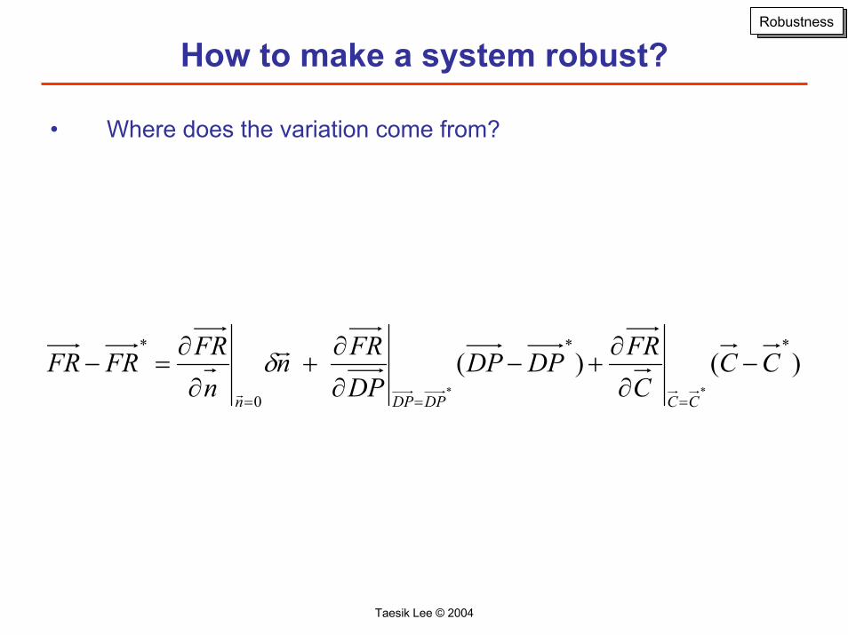
How to make a system robust?
• Where does the variation come from?
)( )( **
0
*
**
CCCFRDPDP
DPFRn
nFRFRFR
CCDPDPn
−∂
∂+−
∂
∂+
∂
∂=−
===
r
r
δ

Taesik Lee © 2004
Robustness
)( )( **
0
*
**
CCCFRDPDP
DPFRn
nFRFRFR
CCDPDPn
−∂
∂+−
∂
∂+
∂
∂=−
===
r
r
δ
0. Assign the largest possible tolerance0. Eliminate the bias ( E[FR] = FR* )
1. Eliminate the variation: SPC, Poka-Yoke, etc.2. De-sensitize: Taguchi robust design3. Compensate
2 31
⎟⎟
⎠
⎞
⎜⎜
⎝
⎛−
∂
∂+
∂
∂−=−
∂
∂
===
)( )(*
0
*
**
DPDPDPFRn
nFRCC
CFR
DPDPnCC
r
r
δ

Taesik Lee © 2004
Bring the system range back into design range: Re-initialization
Robustness
Example: Design of Low Friction Surface• Dominant friction mechanism: Plowing by wear debris
• System range (particle size) moves out of the desired design range ⇒ Need to re-initialize
Figure removed for copyright reasons.
Figure removed for copyright reasons.
N. P. Suh and H.-C. Sin, Genesis of Friction, Wear, 1981 S. T. Oktay and N. P. Suh, Wear debris formation and Agglomeration, Journal of Tribology, 1992

Taesik Lee © 2004
Robustness
Design of Low Friction Surface
• Periodic undulation re-initializes the system range
Figures (6-part diagram and two graphs) removed for copyright reasons.
S. T. Oktay and N. P. Suh, Wear debris formation and agglomeration, Journal of Tribology, 1992