279 - digital scholarship | lehigh university...
TRANSCRIPT

"-
THE MOMENT CURVATURE RELATIONS
FOR
COMPOSITE BEAMS
by
Charles Culver
This work has been carried out as part of an investigation sponsored by the American Institute of SteelConstruction.
Fritz Ehgineering LaboratoryDepartment of Civil Engineering
Lehigh UniversityBethlehem, Pennsylvania
Fritz Laboratory Report No. 279.7December 1960

279.7
i
CONTENTS
l.
2.
3.
4·5.6.
7.
8.
9.
Introduction -
Assumptions
Method of Solution
Example Solution
Summary
Acknowledgements
Nomenclature -
Appendix - - - - - - - - - - - - -
A. Summary of Equations - - - - - -
B. Outline of Example Solution - - -
C. The Plastic Moment of A Composite Beam
Tables and Figures - - - - - - - - - - -
Page
1
2
3
7
13
15
16
18
18
43
4950
279.7
THE MOMENT-CURVATURE RELATIONSFOR
COMPOSITE BEAMS
1. Introduction
-1
Composite beams composed of a concrete slab supported
by a steel wide flange section are frequently used in brdige
and building construction. In order to compute the moment
resistance, deflections, and rotations of the composite section,
the moment-curvature relations must be established. This paper
presents the results of a study to derive equations for the
moment-curvature relations in the elastic plastic region for
a concrete steel composite beam.
In the analysis of the composite section, the Bernoulli
Navier hypothesis (bending strain is proportional to the
distance from the neutral axis) is assumed to h0ld. On this
basis, the effective width of the concrete slab is divided by
the modular ratio "n". This reduces the effective width and
essentially transforms the two element composite section (concrete
steel) to one material, usually steel, since n is taken as Es ..Be
The ~omposite section is then treated as a steel beam un-
symmetrical about the axis of bending.
In the elastic range the ordinary methods of analysis used
in engineering mechanics are applicable for determining the M-¢
relations. After the section has yielded, however, the pene-
tration of plastification or the amount of the beam which has
279.7 -2
reached the yield stress must be determined before thecurva
ture or the moment resistance for any particular strain distri
bution can be computed.
For WF shapes the discontinuities of the cross-section make
direct computation troublesome. In this report a "point-by
point" method is developed for computing M-¢ curves for composite
beams.
2. Assumptions
Tg,e follOWing assumptions were made in order to develop
the moment-curvature relations in this report:
1. The Bernoulli-Navier hypothesis (bending strain is
proportional to the distance from the neutral axis) holds.
2. There is complete interaction between the concrete
slab and the steel beam, i.e., - There is no slip or relative
displacement at the inner face of slab and beam.
3. The stress strain relations for concrete and steel
are those given in Figs. 1 and 2.
"4. The effect of strain hardening is neglected.
"5. The yield s tress is the same for both the web and
flange of the steelbbeam.
6. The tensile strength of concrete is negligible.
7. The beam is subjected to transverse loads only. These
loads lie in the plane of symmetry of the cross section.
8. The influence of vertical shear stress is neglected.

279.7
3. Method of Solution
-3
The first step in the solution of this problem is to
compute the location of the neutral axis or line of zero stress
in the elastic range. Since the neutral axis and the centroidal
axis coincide for sections with one axis of symmetry, this step
involves determination of the location of the centroidal axis.
With the location of the neutral axis determined, the yield
moment is obtained by use of the elementary bending equation
My = ay~~~. The curvature or ¢ at any section in the elasticc
Mrange can then be determined by use 0f the relation ¢ - EI •
With the moment curvature relations in the elastic region
known, the next logical step would be to consider the elastic
plastic region and determine the M-¢ relations in this range.
The analysis will be simplified, however, if the upper limit
of the elastic plastic range, the plastic moment, is computed
first. The plastic moment and the yield moment are upper and
lower bounds for this elastic plastic 'region and with these
bounding values known, the trial and error procedure which will
be used in this region and is subsequently outlined will be easier.
In this report a distinction will be made between the plastic
moment and the ultimate moment. The plastic moment of a section
will be defined as that moment at which the maximum percentage
of the given section is stressed to its capacity.
~~ See Nomenclature pg. 16. for definition of symbols
279.7 -4
Computation of the plastic moment involves consideration
of the strains which the section must undergo to reach this
moment. Thes.e strains put limits on the ratios of the cross
sectional dimensions of the section. If the section is to
develop the plastic moment as defined above the ratios of the
cross sectional dimensions must fall within these limits.
To establish these limiting ratios, a stress distribution
which is compatible with the definition for the plastic m"lD.ment
is chosen, i.e., a stress distribution such that all or most of
the elements of the composite section are working at their maxi-
mum capaclity. By using the relationship between stress and
strain (Fig. 1 and 2) the stress distribution may be converted
into a strain. distribution. Consideration of equilibrium of
horizontal forces· (1 adA = 0) and the geometry of the strain~
distribution leads to various relations or ratios between the
cross sectional dimensions of the composite section such as
the ratio of the area of the steel section to the area of the
concrete slab. This procedure is outlined in Appendix C.
Prior to determining the plastic moment of a particular
section, the ratios of the necessary cross sectional dimensions
are computed and compared with the ranges for these quantities
given in Appendix C. If these ratios fall within the limits
given the plastic moment may be determined by applying the
formula for Mp. If the ratios of the cross sectional dimensions

279.7 -5
do not fall within the limits given the section will fail prior
to achieving the plastic moment. For this case the section
will have failed before the maximum percentage of the cross
section is stressed to its capacity. In this case the maxim~
moment will'be termed the ultimate moment. For most commonly
used composite beams the ratios of the cross sectional dimensions
are such that they fall within the ranges given in Appendix C
and the, formg.la given may be used to compute the plastic moment.
After the quantities in the elastic range and at the
plastic moment have been determined, it remains t6 find the M-¢
relations in the elastic plastic region between the yield moment
and the plastic moment.
The limit of elastic action is reached when either the
outer fibers of the steel beam reach the yield stress and/or
the outer fibers of the concrete slab reach the cylinder strength,
tf~. After reaching this limit of elastic action, yielding
penetrates into the steel beam, the slab, or both. Thus, the
ensuing stress distributions are such that a certain proportion
of the composite section has reached the yield stress. There
are many possible stress distributions for any composite section
in this elastic plastic region. In this report, the moment
curvature relations for the thirteen stress distributions which
are most likely to occur were developed.

279.7 -6
Since the composite section is unsymmetrical about the x
axis the neutral axis must be located in either the upper half
of the web of the steel beam, the top flange, or the concrete
slab. The first step in deriving the equations for the elastic
plastic region is to assume a location for the neutral axis and
a given penetration of yielding into the steel beam and/or slab.
These two assumptions completely fix the configuration of the
particular stress distribution.
The second step is to reduce the stress distribution to
f resultant tensile and compressive forces by multiplying the stress
by the area over which it acts. In order to satisfy equilibrium
at the cross section (1 adA = 0) the sum of these tensile andA
compressive forces must be zero. Reduction of the equilibrium
equation leads to an equation for the location of the neutral
axis in terms of the proportions of the composite section and
the penetration of yielding. The moment resistance for the
stress distribution is obtained next by summing the moments
produced by the resultant tensile and compressive forces obtained
from. the stress distribution.~.' ,
The curvature may be obtained by converting the stress
distribution to a strain distribution and then solving for ¢.The compressive force in the slab or the force which must be
resisted by the shear connection is determined by summing the
resultant compressive forces in the slab.

279.7 -7
The procedure outlined above was used to derive the
equations in Appendix A. A sample of the essential steps in
this process is given for one particular stress distribution
in Appendix AI.
In order to determine the M-¢ relations in the elastic
plastic region, one of the thirteen possible stress distri
butions is chosen and a penetration of yielding into the beam
and/or slab assumed and the location of the neutral axis
determined by using the equilibrium equation for that particular
stress distribution. If the wrong stress distribution has been
assumed the location of the neutral axis will not be compatible
with th~ stress distribution assumed and another trial stress
distribution must be assumed. Since the neutral axis must move
from its position at My to that at Mp only those stress distri
butions which give the location of the neutral axis between
these points need be assumed. This will narrow down the possible
stress distributions from thirteen to approximately four or five.
4. ExamEle Solution
The method of solution outlined in this report for deter-
mining the momentcourvature relations for a composite beam
was used for the composite section shown in Fig. 4. The re- ,~
suIting M-¢ curve is given in Fig. 5. This section was tested
'as part of a research prGgram conducted at Lehigh University on
composite beams. The solution for this section is outlined in
part B of the Appendix.

279.7 -8
The solution in the elastic range for the section in
Fig. 4 located the neutral axis in the top flange at the yield
moment. It also showed that yielding would occur first in the
bottom flange~ This indicated that the solution given in
Appendix A-5 would hold for the initial stage of the elastic
plastic region. Further penetration of yielding into the web
of the steel beam caused the neutral axis to move upward. The
neutral axis, however, remained in the top flange of the steel
beam until yielding had progresseG well up into the web. Since
the stresses in the concrete were still below f~ , the stress
distribution in A-6 of the Appendix would occur next.
Further penetration of yielding into the web of the steel
beam caused the neutral axis to move into the slab and the re-
suIting stress distribution was that of A-IO in Appendix B. As
yielding progressed through the web the upper fibers of the con
crete reached f~ and the stress distribution in A-12 occurred
next. When the yielding of the steel beam penetrated up into
the top flange of the steel beam A-12 was no longer applicable
and the stress distribution was given by A-13. Finally, with the
entire steel section yielded and part of the concrete slab stressed
to f~ the section reached the plastic moment as given in Appendix
c. The equations for moment and curvature obtained for this
section in the elastic plastic range are given in Table I. After
assuming various values for ~ or the penetration of yieldin~ into
the steel beam, these equations were solverd and the results given
in Table II were obtained. These results provided the data for
plotting of the M-¢ curve for the test section.

279.7 -9
Using the M-¢ relations determined for the section tested,
the non-dimensional moment deflection curve shown in Fig. 6 was
obtained and compared with test results. The computed points
were obtained by using the M-¢ relations and the conjugate beam
method to determine the deflections. The solid curve represents
values obtained from test results on the particular composite
section. It. will be noted that the test results are in good
agreement with the computed results.
Of primary interest for any composite section, is the shear
force developed between the slab and beam. This force must be
transmitted by some type of shear connection between slab and beam.
With.the stress distribution at any section known the C force or
compressive force in the slab at that section may be determined.
Fig. 7 shows the value of this compressive force plotted along
the length of the member.
The shear flow, or the force per unit length which the shear
connection must transmit can thenl)be determined from this plot of
C force., Since shear' flow is the change. in C for.ce over a givende . .
l~ngth (q ~ dx ) or the slope of the C force diagram, it may be
determined by differentiation. The C force diagram was plotted
point by point and there is no e.quation to represent this curve.
Therefore a point by point method must be used to determine the
slope of this diagram or the shear flow instead of direct
differentiation. The slope was measured graphically at various
points in order to determine the values of shear flow plotted in
Fig. 8.

279·7 -10
There are several points concerning this shear flow diagram
which warrant discussion. The shear flow in the elastic range
The error involved in such an
and the elastic plastic regions.
the elastic formula (J = ¥cZ'i t is
holds only in the elastic range.
may be determined by using the formula q =Vm • In the elastic:!IT
plastic region, however, the shear flow does not vary in the same
manner as the.external shear and therefore the formula Vm cannotI
be used to determine the shear flow. There has been some dis-1cussion concerning the use of this formula in both the elastic
Since q = Vm was derived fromI
also an elastic formula and
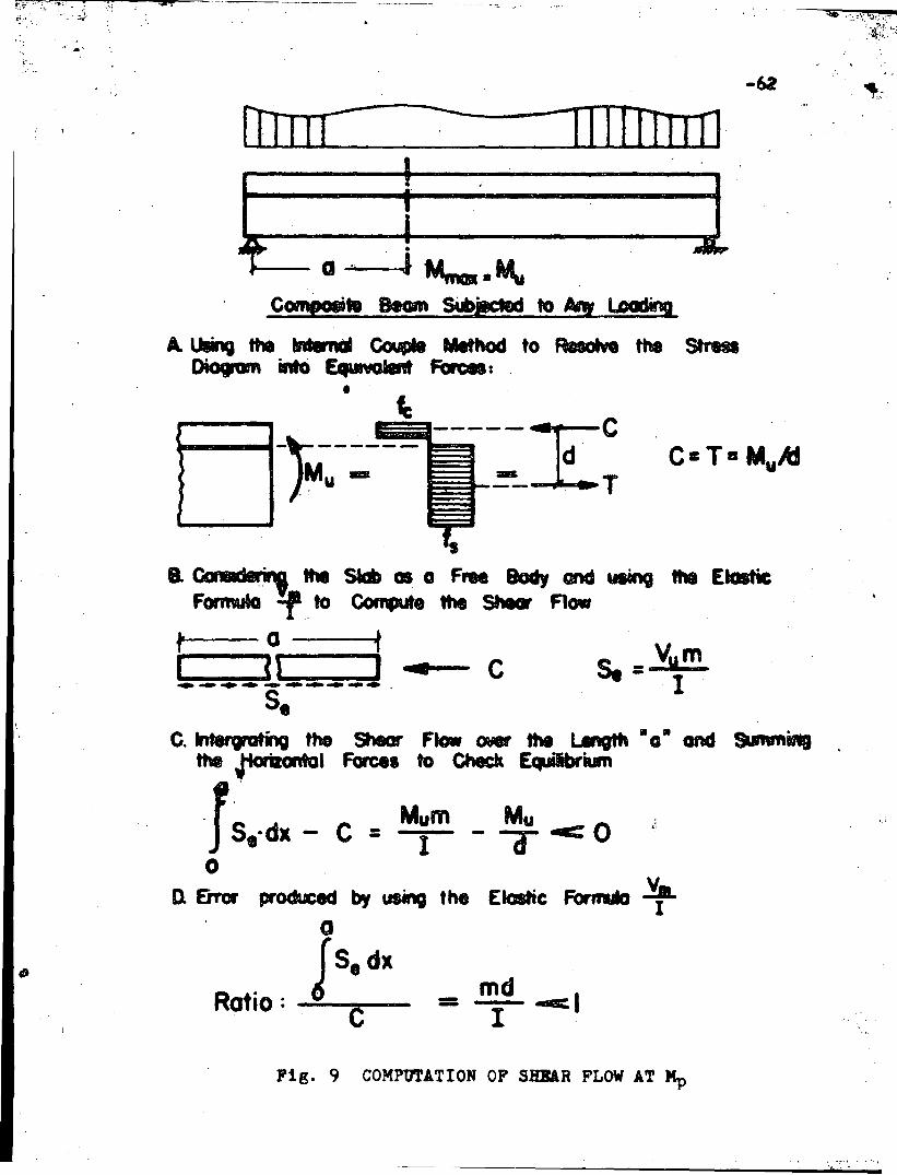
approach is pointed out in Fig. 9.
In Fig. 9 a composite beam is subjected to some arbitrary
loading. A section of the beam from the location of zero moment
to the maximum moment (length "a") is isolated as a free body.
Since in this case the maximum moment is equivalent to tpe plastic
moment, the stress distribution and internal forces at this section
are the same as those given in Appendix C. If the slab over the
length "a" is then isolated as a free body it must be in equilibrium
under the forces shown under Part B of Fig. 9. If the assumption
tha~~"the formula q = ~m may be used in both the elastic and the/
elastic plastic region is correct, integration of this shear flow
over the length "a" must result in a total force equal to the
compressive force in the slab (C) at the ],.ocation of Mp in order
to produce equilibrium. Part C and D of Fig. 9 point
is not the case and therefore the assumption that q =used in both the
outVmI
that this
may be
1 Viest, I.M., Siess, C. P., "Development of the New AASHOspecifications for Composite Steel and Concrete Bridges",Highway Research Board Bull. 174.
279.7
elastic and the elastic plastic regions does not satisfy the
basic requirement of equilibrium. Furthermore, the error
produced by using this formula is not constant for all com
posite beam sections but is a function of the cross sectional
dimens ions. (me).r
The force carried by each shear connector is determined
by summing up the shear flow between two adjacent rows of
connectors·. This is equivalent to integration of the shear
flow diagram between connectors. Again, since there is no
equation for the shear flow a graphical procedure must be used.. ,
The results of this graphical integration are given in Fig. 10
which lists the connector forces •
. It will be noted that the connector forces in the elastic
plastic region are considerably higher than those in the elastic
region. Tests of the strength of individual connectors2 (push
out tests and double shear tests) indicate that the shear
connectors in the elastic plastic region cannot carry these
large forces. One possible explanation for this phenomenon is.,""'" .
tha~ the highly stressed connectors in the plastic region yield
and deform and transmit the excess load (load above the carrying
capacity of an individual connector) back to the less highly
stressed connectors in the elastic region.
2 Culver, C., Zarzeczny, P., Driscoll, G. D., "Tests of Composite Beams for Buildings" Fritz Laboratory Report No. 279.2,June 1960.

279.7 -12
According to this assumption each connector would be carry-
ing the same force at ultimate. If this assumption is valid
then a uniform connector spacing could be used even if the
shear diagram (not to be confused with the shear flow diagram)
varied. The c~nnectors in the regions of high shear would
merely yield and transmit the load to the connectors in the
regions of low shear.
From the above discussion one would expect that shear
connector failure would occur first near the location of the
maximum moment where the shear flow is largest since these
connectors"must deform considerably in order to transmit the
load to the leas highly stressed connectors. On the contrary,.
shear connector failure occurred first near the ends of the
specimens tested.
The analysis discussed in'this report was carried out
assuming complete interaction or no slip between the slab and
beam. In actuallity this case never exists and, slip does
occur. This slip will alter the dllistribution of shear flow
along the member and consequentlr the connector forces. Since
the shear flow is dependent upon the slip distribution, this
slip distribution must first be determined before the true shear
flow and connector forces can be evaluated.

279.7 -13
Any exact failure theory for 'composite beams would involve
an analysis which considers the properties of the shear connec-
tion and the slip or relative displacement between slab and
beam. Until such a failure theory is derived, the shear connec-
tion may be designed on the assumption that each connector is
carrying the same load when the ultimate capacity of the section
is reached. This assumption will lead to a satisfactory design
if a ductile type shear connector, which will permit a re-
distribution of forces, is used.
5. Summary
The M-¢ relations for a composite beam, in the elastic
range, may be determined by the usual methods of engineering
mechanics. In the elastic plastic range, however, a'point by
point method was adopted in this report due to the discontin
uities of the cross section. This point by point method in-
volves a trial and error procedure using the equations deyeloped'?::....,( ...,~~~
for the possible stress distributions over this elastic plastic
range.
The equations derived in this report are only valid for
the case of complete interaction or no slip between the elements
of the composite section. Since complete interaction is never
realized in an actual composite beam, the equations in this

279.7 -14
report provide an upper bound to the solution of the problem.
The development of a failure theory which would consider the
deformations of the concrete slab relative to the steel beam
must be developed before an exact solution to the problem of
the M-¢ relations may be obtainsd.

279.7
6. ACKNOWLEDGEMENTS
-15
This report was prepared as a term paper in partial
fullfillment of the requirements for the Masters Degree in
Civil Engineering at Lehigh University. The work was done
under the supervision of Professor George C. Driscoll, Jr.
This report is part of an investigation on Composite
Design for Buildings sponsored by the American. Institute of
Steel Construction. Work on this project is currently in
progress at Fritz Laboratory, Lehigh University of which
Lynn S. Beedle is the Director and Professor W. J. Eney, Head
of the Department of Civil Engineering.

7.
be-----=---1
•
NOr-tENCLA TORE
-16
-
Section Dimensions, Stres~ Distribution.
Ac
Af
As
be
C
e
--- deI
d s
e
f'c
0 y
I
My
~-I-
m
- area of concrete slab Ac = bcc e
~ flange area of steel beam Af = As - w(d s -2t f )
- area of steel beam
- widt~ of concrete slab
- total compressive force at any cross ••etl'n
- distance from neutral axis of composite section toextreme fiber of steel 1n tens10n
- depth of concrete slab
- depth of steel section
- distance between resultant compressive end tensile forcesat MT)
cy!1nder strength of concrete at 28 days•
- yield stress of steel beam
- moment of Inertia of composIte sect1on, concrete transformedto equivalent steel area
- theoretical y1eld ~oment
- theoret1cal plast1c ~oment
- stattcal moment of transformed compressive c~ncrete areaabout the neutral axIs of the composlte sect10n
n '::"3 teel
E:concrete

-17
7. NOMENCLATURE (Continued)
Q - Connector force
q - Shear flow per unit length
s - Connector spacing along the longitudinal axis of the beam
T - Total tensile force at any cross section
t f - Flange thickness
V - External shear force
w - Thickness of Web of steel beam
a - Location of neutral axis in steel beam
~ Percentage penetration of plastification in steel beam
~ - Location of neutral axis in slab
~ - Percentage penetration of ultimate stress into concreteslab.
- Strain hardening strain for steel ~st = 15xIO-3 in/in.
- Yield strain for concrete ~~c = 1.0 x 10⁻³ in/in.
Yield strain for steel ~ys = ~Es
au - Ultimate concrete strain .~ = 3.0 x 10";'3· in/in.
6 - Deflection of beam in inches.
)_/
-18
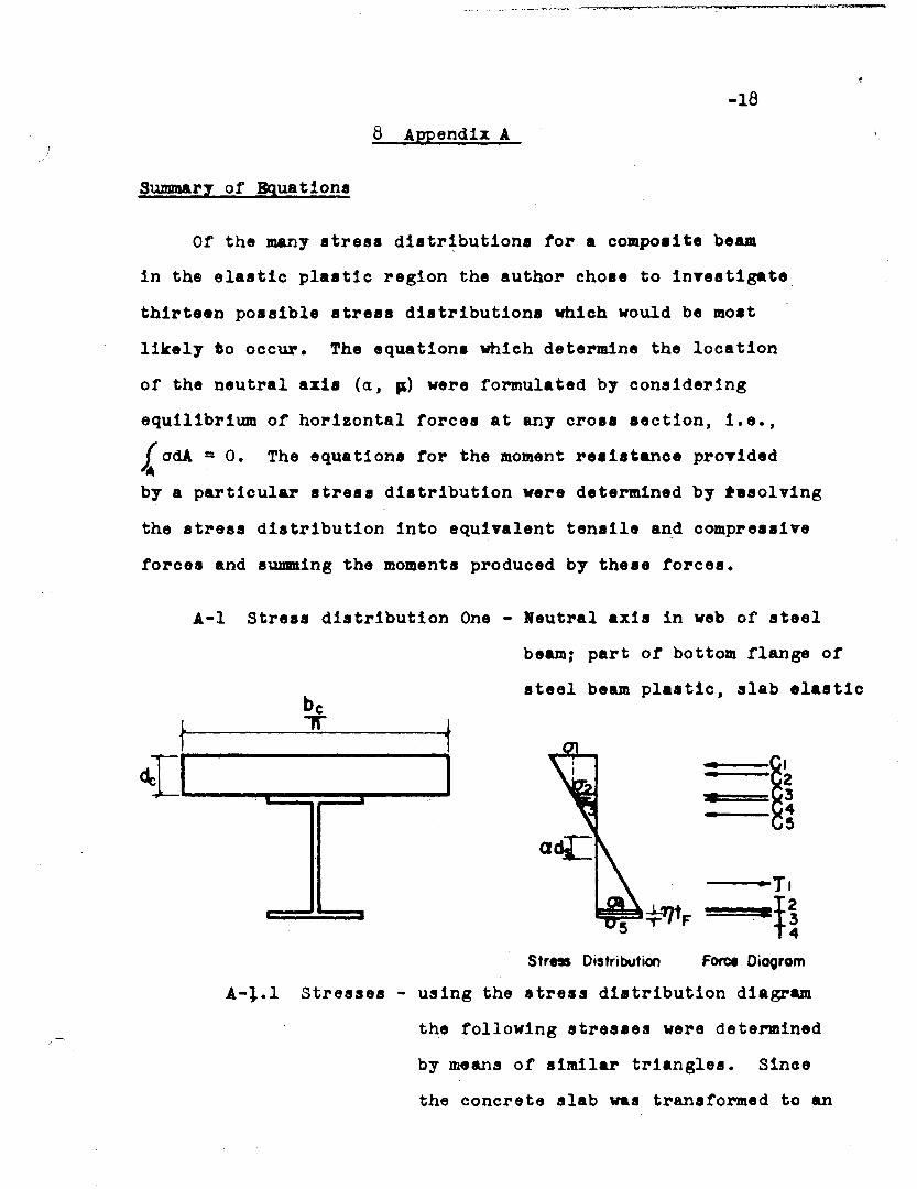
8 Appendix A
SummarI of Bguations
ot the many stress distr~butions tor a compo.ite beam
in the elastic plastic region the author cho.e to investigate
thirteen possible stress distributions which would be mo.t
likely to occur. The equation. which determine the location
of the neutral axis (a, ~) were formulated by considering
equilibrium of horizontal torces at any cross section, i.e.,
J.C adA = O. The equations tor the moment re.istance provided
by a particular stress distribution were determined by tasolving
the stress distribution into equivalent tensile and compressive
forces and summing the moments produced by these forces.
A-I stress distribution One - Neutral axis in web of steel
beam; part ot bottom flange of
steel beam plastic, slab elasticbet-_-...;.:...T__{
~I I
Str.. Distribution
--....•..TI
~~···f!Force Diaoram
A-l.I stresses - using the atress distribution diagram
the following stres.es were determined
by means of similar triangles. Since
the concrete slab was transtormed to an

APPENDIX A -19
equivalent steel area by use of the
modular ratio "n", the stresses 01 and
02 given below are stresses in the
transformed section. In order to ob-
tain the actual stresses in the concrete
of the composite section, the stresses
in the transformed section (01 and 02)
must be divided by the modular ratio "n".
2 + ds _ 2 dsa-:::r-de U c
1 + 2a - 2't) tfd s
cry ( 1
1-2a°2 =
tr <1+ 2a - 2T) -
ds
1-2a - 2 tf
°3 = 0yds
1+2a - 2 tfTlds
1+2a - 2 tfds
1+2a - 2T) t fds
Al.2 Forces - The forces shown in the force diagram
are computed by multiplying the stress by
the area overwhich it acts. For example,
the compressive force Cl is obtained by
multiplying the transformed area of the
slab by the triangular stress distribution,

APPENDIX A -20
Cl = °1-°2 Ac2 n
C2 = °2 Acn
C3 = °2-°3 Af2 2
C4 = ° Af32
the compressive force C2 is obtained by
multiplying the transtormed area of the
slab by the rectangular stress distribution,
C3 and (;4 are the compressive forces in the
top flange resultIDng from the triangular and
rectangular stress distributions, C5 is the
compressive force resulting from·the stress·
triangle in the web above the neutral axis.
The force Tl is the tensile force caused by
the triangle of stress below the neutral axis·
in the web, T2 and T3 are tensile forces re
sulting from the rectangle and triangle of
stress in the bottom flange, and T4 is the
tensile force due to the rectangle of yield
stress in the plastic portion of the bottom
flange.
T2 =~ Af (l-Tj)2'
T3 = 0y-04 Af. (l-Tj)-'2 2
C5 = °3 weds d- a. s - t f )2 2

APPENDIX A -21
Al.a Equilibrium - In order to satisfy equilibrium at the
section, the eqUation~crdA = 0 must beA
satisfied. By equating the sum of the
horizontal forces to zero this equation
is satisfied. Summing horizontal forces,
considering compressive forces positive
and tensile forces negative, and reducing
leads to the following:
[1 + de
ds
Al.4 Location of the Neutral Axis -
Using the equilibrium equation and
solving for a the location of the neutral
axis is determined in terms of ~ or the
percentage of the bottom flange which has
reached the yield stress. For each
composite beam there is a unique value for
a for each value of ~ for this stress
distribution. In order for the equation
to be valid for a particular section, i.e.J
for the particular section to assume this
stress distribution the value of a
determined from this equation must fall
within the prescribed limits and the

,f
-22
APPENDIX A
value of the stress at the extreme fiber
of the slab must be less than nf~. If
after assuming value for ~, the computed
value for a does not fall within the pre-
scribed limits or the concrete stressI
exceeds nfc , this means that the section
cannot develop the assumed stress distri-
butioni
Ac (l+dC ) + Af tf 2nAs -~
1ds 2A s ds
a 2 Ac + Af + wdsc:.:_ 2 wtfnAs As As As
The neutral axis for a composite section must always
to above mid depth of the steel section (assuming symmetrical
rolled steel beams) and since thIDs equation only holds when
the neutral axis is in the web the following limits may be
applied:
o < ~ ~ 1.0
Al.5 Moment Resmstance for Given stress Distribution -
Taking moments of the forces shown in the force
diagram about the bottom flange of the steel beam and
simplifying the equation leads to:

APPENDIX A
Ml tYAsdS ] {Ae(1~ de - 2a d + 2 l~\ +Af
1+2a-2n~~- a c
nA s 'd d$ 3 Ass
1 tf + 2 [:;r +n1. [:;12)+ wds (1 + 2a t f tf+{:~12("2 - - a - a -- 3 6 As ds dsds 6
It will be noted that only the first term contains any
dimensional quantities, all the other terms are non-
dimensional ratios or parameters. Taking the yield stress
in kips per square inch, the area of the steel beam in
square inches, and the depth of steel beam in inches will
result in units of kip inches for the moment.
Al.6 Determinationnof Curvature (¢)
Tan ¢ = :.::ry
Since ¢ is small the tangent of the angle and
the angle itselr are approximately equ~l
ri C' E:. Y'P = ::.::r = ___......-JI. _
.y=
Al.7 Determination of Compressive Force in the Slab
cryA c[ d 1
C = Cl + C2 = l-2a + cn as
1+2a-211 tfUS

oAPPENDIX A
Comment on Method used - The moment equation and
the equilibrium equation contain the unknown
parameters a and D. Using the expression for a
given in A-l.4 the moment equation could be re
duced to a function of D only. This would lead
to a more complicated expression. It is much
easier to assume a given penetration of yielding
(D), determine a from the equilibrium equation and
then compute the moment using these values of a and D.
A-2 .stress .DistributionTwo - Neutral axis in web of! steel be~;
bottom flange arid part of web of steel beam plas.tic,
slab elastic
A2.1 Location of Neutral Axis
Ac (1+ dc ) + Af (D - 1 tf)+ wds (D2+l~r- 2D t f )1 ~ ds As 2 a; As dsa .- -2
Ac + Af + wds (1 - 2 .!f)nAs As As ds
0< 1 t f tfa~-- ~ D......-::2 ds cr;
~2.2 Moment Resistance

APPENDIX A -25
+'n3 t t+ wds (1 - a ~ + 2a -! - f
As b 3 ds as
+ Af (1A 2s
- a2
+ 1 [tf] +.n tf )3 ds 2 as
[t f ]
2
+ 2 ds
-
2 ~:;r)}- 3
A2.3 Curvature ¢
¢2 f. y=
ds + 2 a ds -2T) ds
A2.4 Compressive Forge in the Slab
C = cryAcn
A.3 Stress Distribution Three - Neutral axis in web of steel beam;
part of bottom flange of steel beam plastic, part of
concrete slab at ultim~te strength.
A3.1 Location of Neutral Axis
[Af 2 t f + Ac fill . t: t s
a = 2As T) ds' -A -..9. (- + - :!::l -~ 2. - 11 -! + 2 -'.' {~s cry 2 2n f~ 2n ~b ds
-n s'- t f )Jd s

APPENDIX A
A second equation for a is obtained from the stress
distribution by means of similar triangles.
cr nf1y c=
ds + a ds-Tltf ds ds - ';dc + de- a2 2
a =n2
f11 + n c
cry
The two equations are solved simultaneously for a and
.; by assuming values for Tl. In order for this stress distDi
bution to hold the values' of a, Tl, and s must be within
the following limits:
0< a ~ 1 - tf. "";;;:: 2 ds
A3.2 Moment Resistance
O<i) ~ 1.0 o < s
2ac; f1 de 2fb de - Tl'; f~ t f=-c. -¥3 cry ds dscry cry ds
2T]s f~ de tf2
f~ de tf+ Tls + 1 _3 cry ds ds
-3-Oy ds ds
ai
a - L + E:£ + ~L de - a den 2n n bIi ds 3n ds
APPENDIX A
+ 2as de + ';2 de _a.;2 de + 1 fb + 1 f e de +'2-an ds 6n ds 3n ds cry 3 cry o.s,
f6 de f~ tffe + 2a - g !l de t f ) Afa_ 3" a ds - T) -- +-cry Y cry ds 3 cry ds as As
_ tf + 2[:;]" + ~
3 [:;r)(1 - a + wds (1 - a2 ds :3 'A 6s
_ tf + 2 atf
+ 2 [:~r -~ t:;r)}dsds
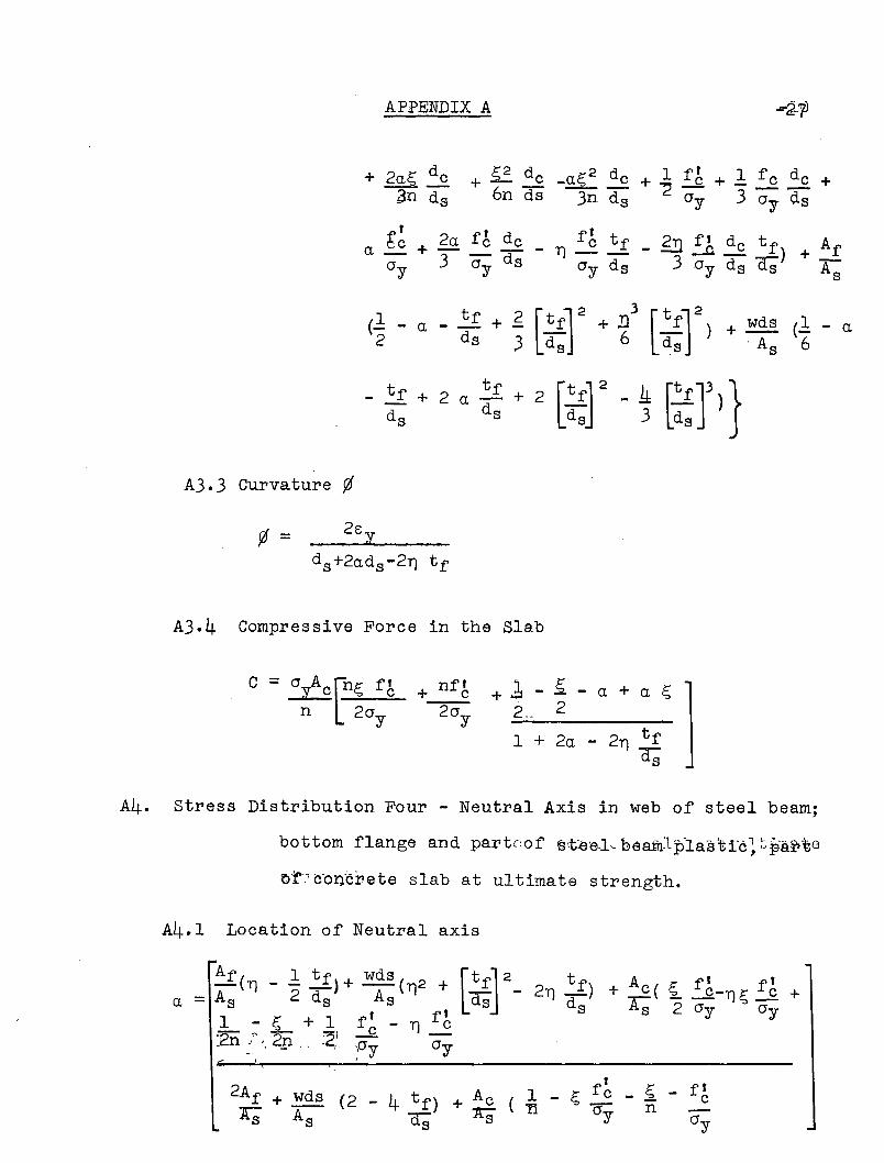
A3.3 Curvature ¢
¢ = 2e y
ds +2ads -2T) tf
A3.4 Compressive Force in the Slab
1 + 2a - 2T) tfcr;
+~-.;-a+a.;], 22 __
A4. Stress Distribution Four - Neutral Axis in web of steel beam;
bottom flange and partc:of s'-t:e'e·l- heafn1plastic ~ ~ paTtG
~yJr,-' c·oncrete slab at ultimate strength.
A4.1 Location of Neutral axis
2Af + wds (2Jr; As
111

APPENDIX A -28
1 + n fba = 2 11_
cry
fl1 + n e
cry
o < a < 1 _ t f-....; 2 ds
A4.2 Moment Resistance
tf-d ::s 11
so <~
+ 2a3
fl de + 11~2 f~ de 1 ID'I + fb - 11fl +-..£ + - .-£. a_ e
cry ds -3- a,y ds . 2 cry cry cry
1 - a + 1 fb de + 2a fb de _ ~ fb de +2n n 3 cry d s 3 cry d s 3 cry ds
as + ~2 de -~ de)n bi1 ds 3n ds
+ Af (1 _
a - tf + 1
[::r+ .!l tf)+ Jolds ( 1 + 2 [::J 2As 2 ds 3 2 d s As 6
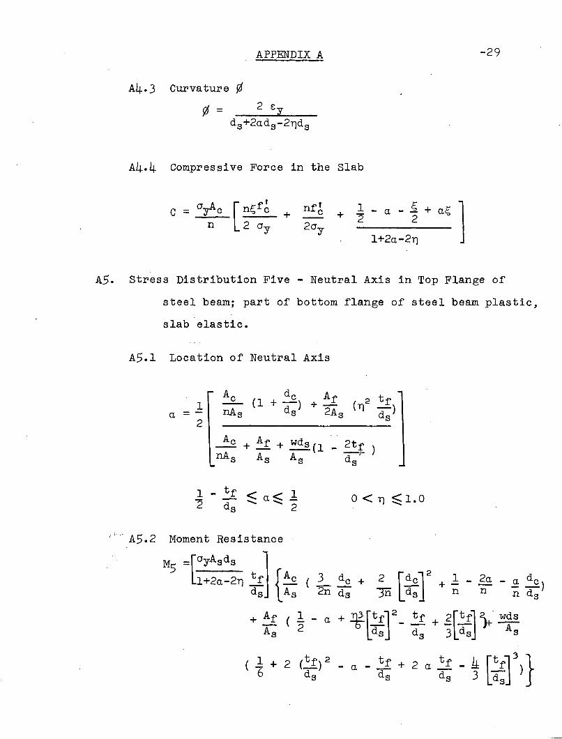
APPENDIX A
A4.3 Curvature ¢¢ = 2 ey
ds+2ads -2T)ds
A4.4 Compressive Force in the Slab
-29
1+2a-2T)
+ nfb 1 - a - ~+ 2 2
2ay
A5. Stress Distribution Five - Neutral Axis in Top Flange of
steel beam; part of bottom flange of steel beam plastic,
slab elastic.
A5.1 Location of Neutral Axis
1a
2
Ac dc Af t( 1 + -) + (2 fd - Y)-)nAs s 2As ds
Ac + Af wd 2t+ _S(l __! )nA s As As ds
1 - tf < < 1- ........ a,2 d s 2
Moment Resistance
M5 =[ayAsds 11+2a-2Y) t f fAc
ds lAs
+ Af ( 1As 2
( 1 + 2 (tf)26 d s - a - ~~ + 2 a :~ - ~ [::] \ }
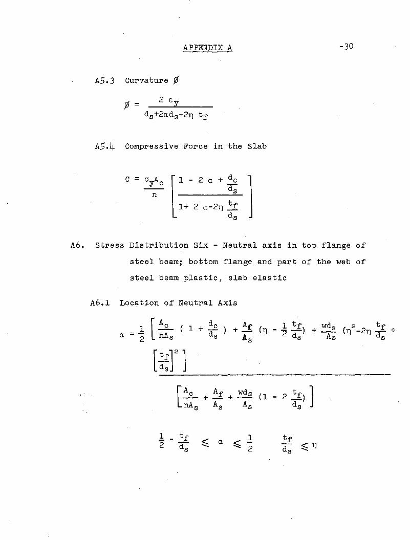
APPENDIX A
A5.3 Curvature ¢
¢ = 2 eyds+2uds -2T) tf
A5.4 Compressive Force in the Slab
C = ayAc 1 - 2 u + dcdsn
1+ 2 u-2T) tfds
-30
A6. Stress Distribution Six - Neutral axis in top flange of
steel beam; bottom flange and part of the web of
steel beam plastic, slab elastic
A6.1 Location of Neutral Axis
= 1 [Ac (1dc ) + A~ (T) 1 tf + wds 2 tf+- - "2 -) (T) -2T) - +
°U2 nAs ds As ds As ds
[::r]" [~ Af wds (1 - 2 t f ) ]+- +--
nAs As As ds
12
1~ 2

APPENDIX A
A6.2 Moment Resistance
-31
M6 =[cryASdS ] Ac1+2a-21') As
~f
As
A6.3 Curvature ¢
- a + 2a tf d s
¢ =
A6·4 Compressive Force in the Slab
C ~ crte [ 1-2 a dc
1+-
ds
1+2 a -21')
A7. Stress Distribution Seven - Neutral axis in the top flange
of the steel beam; part of the bottom flange of the
steel beam plastic, part of the concrete slab at
ultimate strength.
A7.1 Location of the Neutral Axis
APPENDIX A -32
fl fl t + 1 f~I
-S-Ac ( S e - Tls -.Q--! - T) t f f e +.L
As 2 cry cry ds · 2 cry ds cry 2n 2n
a =Af
2tf( Il+- 2 0;As
Ae (1 s fb s f~ ) 2 Af + wds 4 t f+ (2 - )
As n cry n cry As As ds
a =
I f'1 + de - s de - E: f e + n T) ~2 d s d s 2 cry cry
O<T) ~1.0 O<~
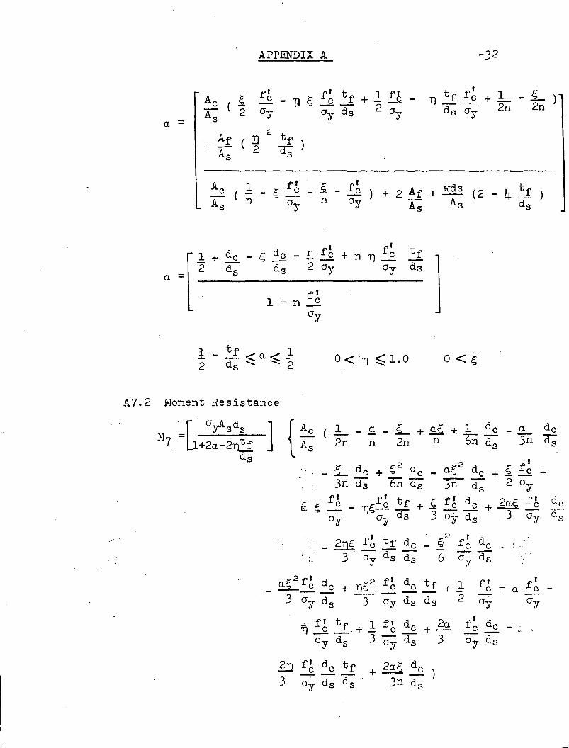
A7.2 Moment Resistance
I+ a f e -
cry
] {~:(1 _.£ _ s... + as + 1 de _ a de
2n n 2n n . 6n ds 3n d s. I
_ L de + S2 de _ as 2 de + s f e +3n d s bIi CIS 3n ds 2 cry
li s fb T)Sf~ tf + s fb de + 2as f~ decry' cry as 3 cry d s 3 cry a;
I . 2 I2'!)s f e tf de _ ~ f e de
,. 3 cry ds d s 6 cry d s
_ as 2fb de + Y)S2 f~ de tf + 1 fb
3 cry d s -:3 cry d s d s 2 cry
~ fl t f 1 ~I d 2a f' d11 -£. _ + _.v e e + - .-£ --.£ -cry ds 3 cry ds 3 cry ds
. [. cr__.A d';I--s sM -
? - 1+2a-2T)tfd s

APPENDIX A -33
+ w~: (i +2 a :~ - :~ - a +2t~;r- ~ (:;r"l}A7.3 Curvature ¢
A7.4 Compressive Force in the Slab
C = 0yACn
~n fh + B f~ +-2 0y 2 0y
1 - s - a + as2 2
. t1 + 2a - 2 T) -f
d s
A8. Stress Distribution Eight - Neutral axis in the top flange of the
steel beam; bottom flange and part of the web of the steel
beam plastic, part of the concrete slab at ultdmllate
strength.
A8.l Location of the Neutral Axis
Ac s ft ft S t . t( _ C - 1'1s c:+ L - - + f c - 7( f c ) + Af (T)
_ 1 t fa = As 2 0y 0y 2n 2n ~Oy 0y As '2-
-;'" ds
+ was (2 [:j2_ tfT) + 2T) -)
As ds
a =1 + dc _ s dc _ n fh + nT) f~
2 ct; d s 2 Oy 0y
1 + n fb0y
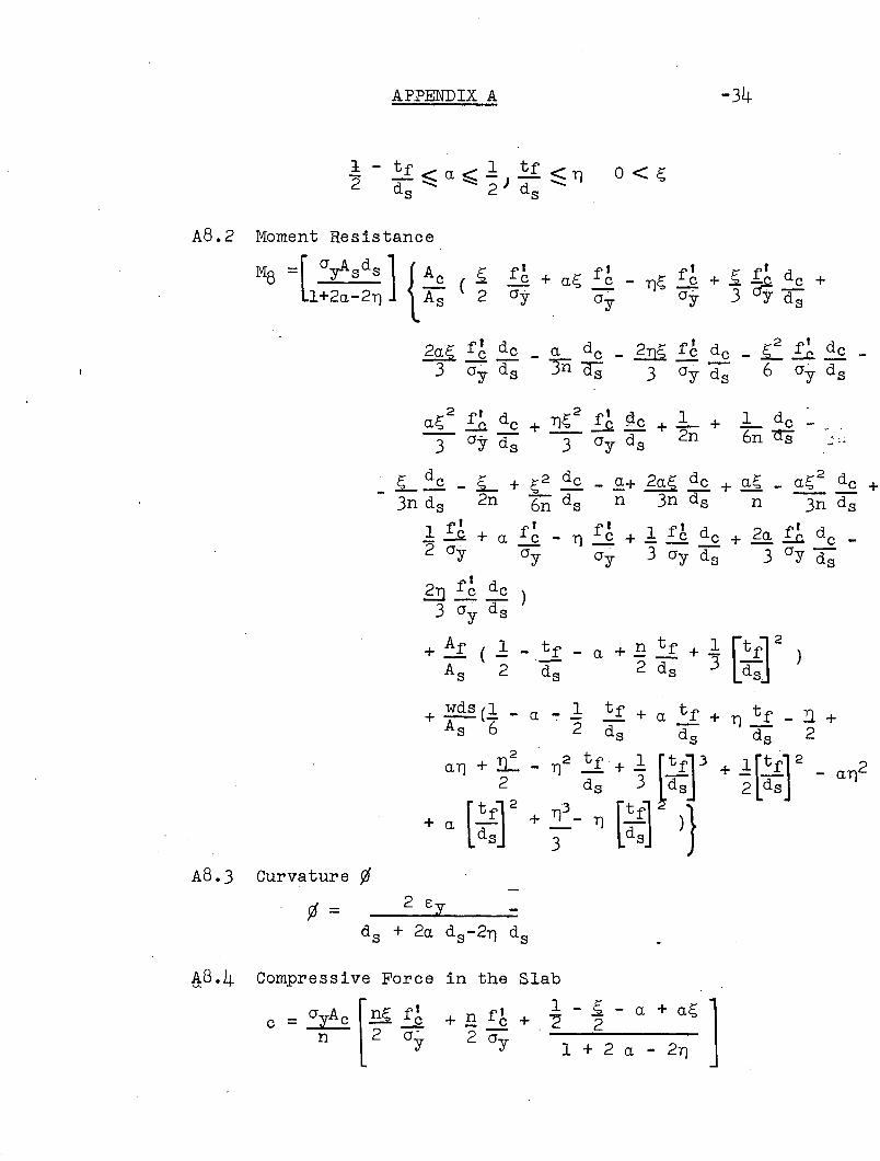
APPENDIX A -34
0<';
A8.2 Moment Resistance
M8 =[ cryAsds 11+2a-2T)
L de -,6n 'ttS
[~;] 2 )_ tf _ a + n t f + 1
ds 2 d s 3
L de _ L + .;2 de _ .£+ 2a'; de + a'; _ a.;2 de +3n ds 2n 6n ds n 3n cr; n 3n ds
f I I f I f I fl d1 ~ + a f c - T) --.£ + 1 ~ de + 2a..::..c. c-2 cry cry cry 3 cry ds 3 cry ds
,g f; de3 cry ds
+ Af ( 1As 2
+ T) t f - II +ds 2
1 (t f ]2
2+ - - - aT)2 d s
3
+ ~(l _ a-I tfAs 6 2 ds
aT) + :!f - T)2 tf2 d s
:3+ T) - T)+ a
A8.3 Curvature ¢¢ = 2 f,y
ds + 2a ds -2T) ds
A8.4 Compressive Force in the Slab
c = (J'l.Ac [~ f'~ + !l fb +1 - .; - a + a'; ]2 2
n 2 cry 2 cry1 + 2 a - 2T)
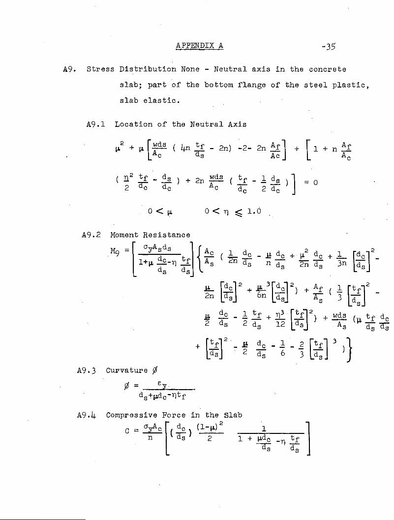
APPENDIX A -35
A9. stress Distribution None - Neutral axis in the concrete
slab; part of the bottom ~lange of the steel plastic,
slab elastic.
A9.l Location of the Neutral Axis
2 [WdS 4n tf - 2n) -2- 2n Af] [1 + Afl.L + lIJL- + n_Ac as Ac Ac
( n2 tf _ ds ) + 2 wds ( t f _ 1 de) ]n -- = 0
2 ~ dc Ac dc 2 dc
0<1tJI. 0<11 ~1.0-...;: .
A9.2
A9.3 Curvature ¢¢ = Cy
ds +lIJl.d c -11t f
A9.4 Compressive Force in the Slab
C =~ [( d c ) (1-l.L) 2 1 1n ds 2 1 + lJ.dc -11 tf
---a; d s

APPENDIX A -36
AIO. stress Distribution Ten - Neutral axis in the concrete slab;
bottom flange and part of the web of the steel beam
plastic, slab elastic.
AIO.I Location of the Neutral Axis
lJ,2 + lJ, [~ (4n. tf - 2n) - 2 - 2n Af ] + I r
A c as . A c
Af d+ _ (nT) 2-A c d c
n d s _ 12 tf)dc 2 d c
I. ( ":
o < ~
+ wds (n tf tf - 2nT) tf _ n ds + nT)2 ds +Ac ds a;;- dc dc dc
2n tf) = 0d c
AIO.2 Moment Resistance
MIG = ( CYASdS] ee ( .L de + .L [der_~ de - JL [derI +lJ,dc-T) As 2n ds 3n ds Ii ds 2n ds
ds 2
+ t,;3[::T) 2+JI!L dc Af ( I tf
2n +-ds As 6 ds
I tf .H dc + 1) t f ) + wds (1)3 _ I +-- -
·2 ds 2 d 4 ds As 6 6s
.n [tf ]22 d s

APPENDIX A
AIID.3 Curvature ¢
¢ :: ey
ds+lJl.Clc -T)ds
-37
AIO·4 Compressive Force in the Slab
C = a~e~ de2
1(1- Ho) 1
n (T) 2 1+lJ.dc-T)sds
All. Stress Distribution Eleven - Neutral axis in the concrete
slab; ,part of the bottom flange of the steel beam
plastic, part of the concrete slab at ultimate strength.
All.l Location of the Neutral Axms
2 . [ Af cr d tf d cr t cr ]IIJl. + IIJl. 2 - :::.Jl -l[; + ~ - T) - - 1 - ~ (4 ;t. ....f - 2~Ac f~ dc dc Ac f c ds f c
s ds - ds +T) S tf + tf :: a.,. T)-\,~ dc dc dc dc
l-s f' ds T) tf- n c -- dcIIJl. :: cry dc
1 + n f'--2.cry
O<T) ~ 1.0. O<s

APPENDIX A
All.2 Moment Resistance
-38
~ ~ d _ r 2 d d( ~ + ~ C 2 C + 2!IJLS --.£ +
2 3 d s 6 d s 3 d s
All.3 Curvature ¢
¢ = ey
ds+~dc-YJ tf
All.4 Compressive. Force in the Slab
C = fl A [1 + S - .lI!!-2 ]c c 2 2
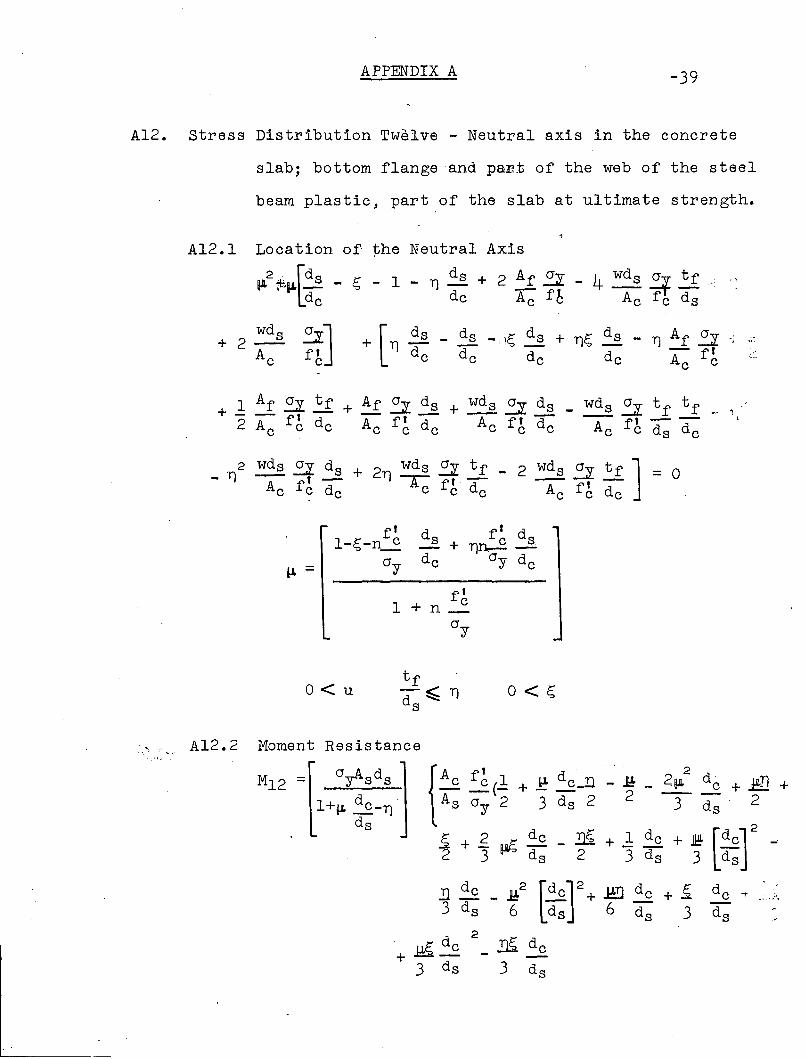
APPENDIX A -39
A12. stress Distribution Twelve - Neutral axis in the concrete
slab; bottom flange and par.t of the web of the steel
beam plastic, part of the slab at ultimate strength.
~he Neutral AxisA12.l Location of
2 . ~dsUft "'" _II"" ~'Il
d c
:!:i.Jftc+ [,., ds _ ds -,]'; ds + 11'; ds - 11 Af 2
'I d d - ftc c dc dc Ac cc.
+ 1 Af :!.:f.. t f + Af 2. ds + wds :!..:Jl. ds wds :2. t f t f2 - ft Ac fb dc Ac fb dc ft --A c dc Acc . c ds dc
2 wds :!]I ds + 2 wds ~ t f 2 wds 2:l tf' J 0- 11 - t- 11 Ir: ft- =Ac f c dc c c dc Ac f~ dc
O<u 0<';
A12.2 Moment Resistanceref'~ 1 d· 2- J; 21!J1. dc + If.U..n +--(- + Il.I. ....£_n
2 --As a 2 3 ds 2 3 ds 2y
~ + 2 ~dc _2:& + 1de + .II!! [der
2 3 ds 2 3 ds 3 ds
.!l dc ~2 [de)"dill de + S dc "t ~,: . _~:J..
3 ds - 6 ds 6 ds 3 ds2
, lOt:' d c+~-
3 d s

APPENDIX A -40
+ 2)3
6
) + Af (1 [tf ]2
_
As 6 Lds
Wds ( dc t f+-- \t.Q.As <IS ds
2
+U6
~2
6
J!. dc _ 1 tf + 2) tf )2 ds 2 ds 4 ds
- ~ :~ + [~W- ~
A12.3 Curvature ¢¢ = 8 y
ds+lJLd c-Y)d s
A12.4 Compressive Force in the Slab
C= f 1A (1 + ~ - ~]? c 2 2 2
A13. Stress Distribution Thirteen - Neutral axis in the concrete
slab; bottom flange, web and part of top flange
pla~tic, part of concrete slab at ultimate strength.
A13.1 Location of the Neutral Axis
- Y) ds + 2 Af :!.::L + wds ~ (2-4 t f )]dc . Ac f t Ac f c ds
+ Y)c; d s + Af:!.JL (2 ds _ 2)2 dsds _dc Ac fb dc 2 tf dc
+ wds ~ dsTT (2_Ac t dc

APPENDIX A
f' d s f' d s1-S:-n --£ + T)n -.£cry de cry del.L =
1 + n f'-e
cry
-41
0< [lJl.
A13.2 Moment Resistance
0< s:
2 de _ .!l +
ds 2
J:!!:Il + 1 de +.l& [der- .l!2 [::f-2 3 d s 3 d s 6
11 de + .1!!J de + Jfs. [der-~ de _
? d s 6 d s 6 d s 6 d s
lJ.3 [def+ J6 de Af ( 1 d s 1-) +- - -6 d s 6 d s As 6 tf 2
lL'> d s _ J:!. de +Il - .!l ~ ) + wds+ 12 tf 2 d s 2 4 tf As
( t _ 1 - J:!. de + iIJI. de t f +~-TJ t f l}.fds 2 2 d s ds d s d s

APPENDIX A
A13-3 Curvature ¢
¢ = 8 yd s + ~ dc-T) d s
A13-4 Compressive Force in the Concrete Slab
-42

.. '. '...... __ ..... ,_ 1 ••_"
>""
."-" --~.•.- '-_.:~,~,_ .. . ,'~. .
APPENDIX B -43
..
Outline of Example Solution
The moment curveture relations were determined for the
section shown in Fig. 4. An outline of the solution for this
sect~n:follows:
Step 1 - Location of Neutral Axis in the elastic range and
deteM'/1ination of the moment of inertia of the
sectton.
I
- IA yY = IA =
.- NA
-y
= 11.60 in.
I = J y2 dA
A
= 587.7 In4••
steP 2 Determination of the yield moment l~~)
CJ = Mer= ()9) (587.]) =
11.601975 k-in.
Step 3 Determination of the curvature at My (¢y)
¢ = MEI
¢ =~ =YEI
1975 = 112.0 x 10- 6 radians(30,OOOxl0 3 )587.7
..
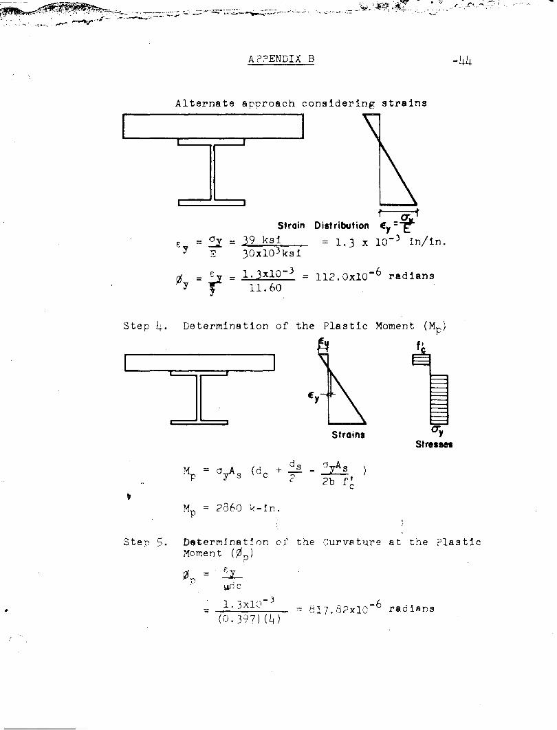
APPENDIX B -44
Alternate approach considering strains
f a; ~Strain Distribution Ey=Y
€y = ~ = 39 ksi = 1.3 x 10- 3 in/in.E 30xl0 3 ksl
¢v = ? = 1. 3xlO- J = 112.0xlO-6 radians
" 11. 60
Strains
Step 4. Determination of the Plastic Moment (Mp )
f'
'JyA s2b f'c
Mp = 2860 k-in.
of the Curvature at the Plastic
~ic
1 3 1 ,-3. x ~.
= ------:---(0.397) (Ld
Step 5. DetermjnationMoment (~p)
¢ = !2-r
., -, -6 'i= d17.b?xlO raa ans

.- .<.. -- .....,~-- -.....
APP~DIX B -45
Step 6. Determination of the possible stress distribution.in the elastic plastic region.
The neutrsl axis in the elastic range and at the yield
moment 1s in the top flange of the steel beam. The stresses
in the extreme fibers of the steel section and the concrete
slab at the yield moment are 39 ksi and 1.46 ksi respectively.
The neuUral axis 13 in the slab when the section reaches
the plastic moment (step 4). Since the neutral axis must
move from its position at My to that at Mp, the possible
stress distributIons in the elastic plastic region between
My and Mp are stress distribution 5,6,7,8,9,10,11,12 and 13.
Step 7. Solution of the possible stress distributions inthe elastic plastic region.
A. Stress distribution 5. The equatiDn for a issolved and yields
•
a = 0.4711 + O.0016~2
For this stress distribution ~ has the limits
O<Tj ~ 1.0

Step 7 (Cont'd)
APPENDIX B -46
By assuming various values for ~ between zero and one
we see that a varies between 0.471 and 0.473. Using the
values obtained for a and ~, the Moment, e Force, and
curvature are determined.
These yalues are listed in Table II on page ~. The
stress in the*extreme concrete fiber with a = 0.473 and.~ = 1.0
is 1.49 ksi.
B. Since the neutral axis is still in the top flange
(a~0.5) and the concrete is elastic, it is easily seen that
the next stress distribution is stress distribution 6 .
•
• By assuming various values of ~ starting with ~ = 0.033
~ see that ~ = 0.2813 when a = 0.5. At this point the
neutral axis Moves into the concrete slab. The stress in
the extreme concrete fiber with a = 0.5 and ~ = 0.2813 is
1.85 kai .

APPENDIX B -47
c. The next stress distribution i8 therefore strea.
distribution 10.
By assuming various values of ~ starting froM 0.2813,
values of ..., which give the position of the neutral axis
are determined. The limit of application of this equation
is the point at which the stress in the extreme concrete,
fiber reaches f c or 3.6 ksi. The values for ~and ~ to
cause the extreme fiber of the concrete to reach f' arec
r 0.279 and 0.83 respectively.
The neutral axis is now in the concrete slab, the,
extreme concrete fibers have reached f and the steel beamc
has yielded to 0.83 of its depth.It
D. stress distribution 12 is therefore the next stress
distribution .
•
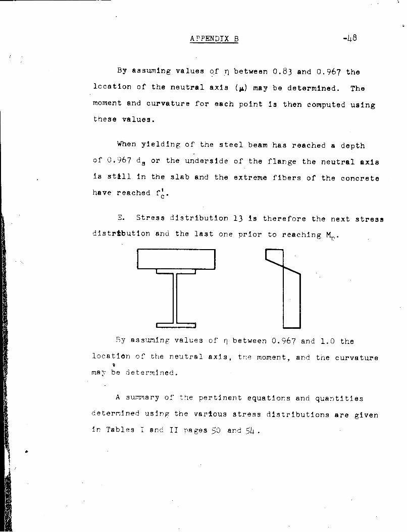
APPENDIX B -48
By assuming values ~f ~ between 0.83 and 0.967 the
location of the neutral axis (~) may be determined. The
moment and curvature for each point is then computed using
these values.
When yielding of the steel beam has reached 8 depth
of 0.967 d s or the underside of the flange the neutral axis
is still in the slab and the extreme fibers of the concrete
have reached f~.
s. Stress distribution 13 is therefore the next stres!
distrtbution and the last one prior to reaching ~.
..
By ass~~ing values of ~ between 0.967 and 1.0 the
location of the neutral axis, tne moment, and the curvatureQ
may be oeter~ined.
A sunmary of the pertinent equations and quantities
determined usinf the various stress distributions are given
in Tables I and II nages 50 and 54 .

APP~DIX C -49
The Plastic Moment of A Composite Section
Plastic Moment - Case I (Neutral Axis in Concrete Slab)*
strains
E<E,t
Strains. Sf,....
., C
- ......~T
Fore"
EquilibrlUlI1 ~
=
Ey < e .~ Est
Sst ~ (::l1+Ey) d s + Eyd c
fibc x = cryAs
LEi tlng Ra tio
As f6Ac ~ cry
Plastic MOMent
(E\1+Cy)
(sst-Sy)
t'\, = T d S + n__ ~ )-~ 22
.:~ Taken from notes of Bruno Thurllmann CE4ll "Selected Topics inConcrete Structures".

TABLE I
Spmmary of Equations Obtained in Example Solution
,"1. Stress Distribution Five
A. Location of the neutral axis2
a = 0.4711 + 0.0016n
o < TJ ~ 1.0
B. Moment Resistance
M5 = [3714.42 J {3. 82375-5.91844a}
1+2a-!L J15
C. Curvature2.6 x 10-3
91=------11.95+23.9a-0.8TJ
-50
D. Compressive Force
k'bt
C = 748.8k 3 -2 a
1+2a-0 .066TJ
2. Stress, Distribution S%i
A. Location of the neutral axis
]
2a = 0.4694 + 0.0939TJ + 0.05277TJ
0.033 ~ TJ
B. Moment Resistance
M =r 3714.421 {4. 1371 - 6.59 a + 0.1187TJ3 + 0.010 7TJ}6 Ll+2a-2TJ J

Table I (Contfd)
2. stress Distribution Six (Contfd)
-51
¢ =
C.
D.
Curvature ¢2.6 x 10⁻³
11.95+23.9a-23.9D
Compressive Force
C = 748 •8kr~ -2a 1li+2a-2D "J
3. stress Distribution 10
A. Location of the neutral axis
~2 _ 2.83~ + 0.448D2
+ 0.7973D - 0.2586 = 0
B. Moment Resistance
_ [3714.4
2]MI0 -
1 + JI!. -D3
C. Curvature
¢ =11.95+411J1. ,-11.95D
D. Compressive
C = 124.8
Force
[
(1-1J.) 2 ]
l+J!-D3
4. stress Distribution 12
A. Location of the neutral axis2 . 2~ + IIJI. 3.57 3.947D + 2.6759D -3.9266D + 1.2558 = 0
s = 2.769D - 1.923~ - 1.769

Table I (Conttd)
4. stress Distribution 12 (Cont1d)
B. Moment Resistance
"
-52
[3714.42 ]M12 =1 + ~-T)
3
1.278 - 1.344T)+1.349s -1.349T)s
-0.944~-0.531~2+1.266~T)+0.572~
222+0 •122iJ. T)-O .122~T)S -0 .122~ +0. 122T)S
+~. 0411!J.2S -0. 041~2-0.041114.3+0. 06T)3.
C. Curvature,1. 3xl0-3 ',
¢ =11. 95+4QJ1.-11. 95T)
D. Oompressive Force
C = 691. 2 [~ + ~ - ~]
5. stress Distribution 13
A. Location of the neutral axis
QJl.2 + ~ [3.5707-3. 947T)J -1.756T)2+4.6427Tl-2.8856= 0
S = 2.769T) - 1.9231!J. -1.769
B. Moment Resistance
\
M =[3714.4
2 J13 1~-T)
3
21.349s + 0.57 ~-1.349 T)S + 0.122 T)S
2' 2-0.122S -0.041~ +4.161-9.944~
2 2-0.5327~ -5.833T)+1.230~T) +0.041QJ1. S
-0 •1229ilJl.DS-0. 041~3+0.'1229.iA-211+1. 66T)3 '
C. Curvature
¢ = 1 ..Jxl0-3
11. 95+41J.-11. 95T)
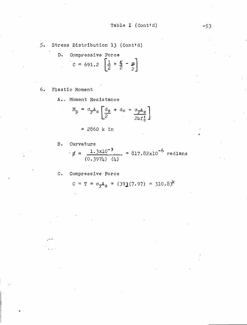
Table I (Conttd)
5. stress Distribution 13 (Cont1d)
D. CompressiveForce
C = 691.2 [1 + ~ - ~]222
6. Plastic Moment
A•. Moment Resistance
= 2860 k in0,
-53
B. Curvaturel '.3xlO- 3
- ¢ =(0.3974) (4)
C. Compressive Force
= 817.82xlO-6 radians
C = T = ayAs = (391(7.97) = 310.8jk

TABLE II
SUTJIT·fARY OF VALUES DETERXmifED FR()r~ THE VARIOUS STRESS DIS'!'RIBurI'IONS
StressCurvature Compressive
7Jds a ~. r4:oment f6 Force in SlabDistr1- (in) (k-in) (radians Cbut10n 10-6 ) (kips)x
0 0.47100 0 0 My =197$ 112 •.0 1$1.56
0.0198 .47167 0 0 2014.36 114.3 152.08.0264 .47210 0 0 2022.64 115.1 152.73.0330 .47270 0 0 2028.69 115.8 153.23
1.195 .47932 0 0 2068.94 123 .. 75 1$8.12
6 1.793 .48467 0 0 2102.99 130.33 161.782.96'8' '.49636 0 0 2166.41 145.. 74 169..203.362 .50000 0 0 2190 .. 70= 151.34 171.92
4.780 0.0470 0 2245.31 176.68 183.955.,975 .0921 0 2307 .. 40 204.94 193.81
10 7.170 .1410 0 2384.12 243.26 206.028.36$ .1970 0 2455.47 297.28 219.869.560 - .2590 0 2548.24 379.t(.5 239.609.919 - .2790 0 2578.01 412.96 246.65
10.397 - )'"' c't" 0.0525 26.36.20 468.38 258 .. 16• V--,;J
10.755 - .3245 ~0990 2660.58 521.46 267.7012 10.994 .3350 ~1338 2693.46 566.20 276.06
11.233 .3450 ~1706 2746.76 619.93 285.3311.556 ~3563 ~2235 2774.40 714.44 299.70 I
11.592 .3549 .2344 2810.00 730.. 91 303.95 ¥113 11.711 .- .3591 .2541 2835.00 775.9~ 30<1.35
Mp 11.950 - .3974 .2968 2860.00 817.82 310.83

l'c
;.- .
Eyc =0.001 in/in.
Strain
-55
•
Fig. 1 -STRESS-STRAIN RELATIONS FOR CONCRE'I'E
IL- --L-=------------.......~EsEys =i Est=0.015 'rr.n
Strain
Fie> 2 - ST:{SSS-S'l'iiAIN RELATIONS FOR 513;EL

®Neutral Axis in the Web of the Sttel aeam
Neutral Axis in the Top Fla"9G of the Steel Seom
13@,(@)
Neutral Axis in the Concrete Slab
Fig. J. STRESS DISTRIBUTIONS IN THE ELASTIC-PLASTIC RANGE
I
I

f"""--------b::;..z.c------f-57
-Ill
•
•
Concrete Slab: Ratios:
be = 48 In. de =11 = 0.33da . 12de = 4 In.
f'ds _ii= 3.0
= 3600 psI de - 4c
Steel Beam: de -L = 10Tf - 0.4
Section - l2WF27
As 7.97 1n"" ds 12 = 30:: :::-
tr 0.4wd s = 2.87 in 2
tr =~ = 0.033ds = 11. 97 In. ds 12
f y = 39.0 kal Ac = ill- = 24Af = S·29 1n 2 As 7.97
Compo~1te section: tf = 0.4 = 0.10
1n4 de 4I = 587.7
1n3 f'=~45.1
e = 0.092m =0y 39
n = 10Af = .i:.£i = o. 6637As 7.97
wdj = 2.67 ::: 0.3601As 7.97
Fig. h Dimensions of Composite Section Used1n Example Solution
•
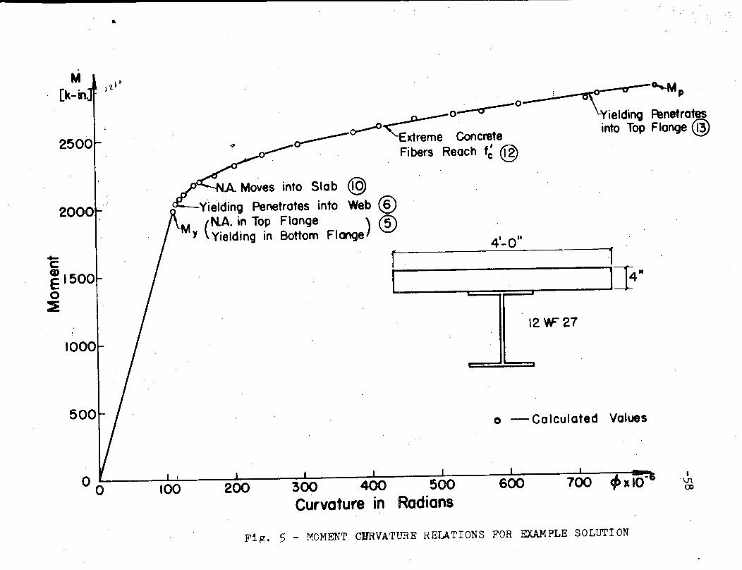
.M
[k-in.
2500
___--O----J.---~~~~o--O""M p
0--"~o- 0 ~Yielding Fenetrates
cr--- 'Extreme Concrete into Top Flange @. . Fibers Reach f~ @
12 w: 27
...-.----c::=::=T'----1"·1
600
o - Co Iculated Values
4'-0"
300 400 500Curvature in Radians
200100
500
1000
2000
~cE1500o
::E
Fig. 5 - !10MENT CIJRVATURE RELATIONS FOR EXAMPLE SOLUTION

•
".,;
.l!
:!:!1.5CD.->-..
0
§1.0
~..............cCD 0.5E0~
*'0
0
_-0...0-------
---~--- Computed Resultso Test Results
2 3 4 5 6l Deflection / l Deflection at Yield
Fig. 6 COMPARISON OF COMPUTED QUANTITIES AND TEST RESULTS

l I1
12 YF 27 !•• ~ I.- l .- 4
,T.st Specimen"
C[K]
·G
J.. ,1·a .!--(,eo
(,)
Moment 0iaQIam
234 5Diatance from Support in Feet
•
G
, .
I
Fig. 7 VAR!ATION OF THE COMPRESSIVE FORCH IN THE SLAB

q[k/in]
10·11
8
~o-u...
ba 6oG)
.c:.C/)
4
2
15
t62 4
Distance From Support In Feet
OL...----....L.----..L.------I....---_--L... ---'- ---l__--.JL-L.-----lo
Fig. 8 VARIATION OF SHEAR FLOW ALONG THE LENGTH OF THE SPECIMEN
____IIIiIIII _
~~'¥ ~" .';'" -~~, ~ ':' .t:~ .... :,: ' '.- -' ;j.
',;-62
IIlIrC_=-------_---_TIIIDrrD·
·rr • ....,a -, I
,.'
~_ = Vym~ I·C
produced by using the Elastic Forrmla Vra
l Se dX
Ratio: . C = md -e II .
a ca__." the Slab as a Free Body and using thI ElasticFormula !f. to Compute the Shear Flow
t a iL_.._U J ....4--s.
c. lnterQrotinQ the Shear Flow CMW the lInV,,,·G• and SWftmiftg .the ~atal Farces to Check Equilbrium
-Is' d C Mum Mu 0 ,;.. x- = I -Te:o
D. Eircr
F1g. 9 COMPUTATION OF SHBlR FLOW AT Mp

Q(klin]
10
.8o-LL
S\..--.,.-
7.562 4Distance From Support in Feet
0"'"'-----..4----....A-.---~-----..I-----.L---~-...&--------&----'
o
0 0 0 0 0 0 0 0 0 0 0.. Q • Q .. • • It D • •- - - - - - N N N t.e ~ e 0 e ~ E <II I: ~-• - CD I(Jl ~ (II (Jl (Jl UI Ull (,II N b
•I
Q II Connector Force in kipslconnector
Pig. 10 CALCULATtD CODWECTOR FORCES AT ~
: ~.