215 ghz for monitoring ice clouds: 2.2 feasibility of a …swrhgnrj/publications/synergy.pdf2.2...

2.2 Feasibility of a spaceborne dual-wavelength radar at 94 GHz and215 GHz for monitoring ice clouds:Comparison with radar/lidar synergy

2.2.1 Introduction

The proposals for cloud-profiling satellites by ESA and NASA have both considered a payload of a94 GHz radar and a visible lidar; the very different scattering behaviour of the two instruments wouldenable aerosols, rain, and cloud of all types to be detected. In section 2.5 we will show how lidar andradar can be used to infer the presence of supercooled water layers embedded within ice clouds, but themain intended synergetic use of the two instruments is in the retrieval of the microphysical characteristicsof purely ice clouds; because the radar return is approximately proportional to the sixth power of diameterwhile the lidar echo is proportional to the second, the radar/lidar backscatter ratio is a potentially verysensitive measure of crystal size. Preliminary demonstrations of the retrieval of ice cloud parametersby this method have been presented by Intrieri et al. (1993), Donovan et al. (1999) and Donovan andvan Lammeren (2000). The main problem to overcome is attenuation of the lidar signal, which can besubstantial and is difficult to correct for given the uncertainty in the extinction-to-backscatter ratio. Fromspace the occurrence of multiple scattering can also significantly degrade the retrievals. The penetrationdepths of a spaceborne lidar signal are estimated in section 2.3. In this section we take a differentapproach and examine the potential of dual-wavelength radar for the quantitative determination of icecrystal size and ice water content (IWC). In particular the combination of 94 GHz and 215 GHz isconsidered.

The use of dual-wavelength radar for measuring mean crystal size in cirrus was first proposed by Ma-trosov (1993); the longer wavelength radar scatters in the Rayleigh regime while the shorter wavelengthradar scatters in the Mie regime such that the dual-wavelength ratio (DWR), defined simply as

DWR � 10 log10

�Zl

Zs � dB (2.1)

(where Zl and Zs are the radar reflectivity factors, in mm6m � 3, at the longer and shorter wavelengthsrespectively), is directly related to size. The estimate of size then enables IWC to be estimated moreaccurately than would be possible with a single radar. The technique has been demonstrated usingobservations at 35 GHz and 94 GHz by both Sekelsky et al. (1999) and Hogan et al. (2000a). However,for the typical range of crystal sizes found in cirrus, DWR tends to be less than 4 dB at these frequencies,and for crystals with diameters smaller than around 150 µm is generally to small to be measurable. Thisproblem could be solved by using higher frequencies, for which DWR would be higher for a given crystalsize, but for observing cirrus from the ground such instruments tend not to be feasible because the higherfrequencies suffer much stronger attenuation by both boundary-layer water vapour and low-level liquidwater clouds. Figure 2.1 shows the variation of attenuation coefficient with frequency in dry and humidatmospheres. The only meteorological radar constructed with a frequency above 95 GHz that the authorsare aware of is the 215 GHz described by Mead et al. (1989). They presented observations of low-levelfog, but attenuation was found to be too great to make quantitative measurements in ice clouds.

From space, however, the problem of penetrating the strongly-attenuating moist boundary layer disap-

ESTEC Contract 13167/98/NL/GDStudy and Quantification of Synergy Aspects of the ERM March 2000

3

0 50 100 150 200 250 300 35010

−3

10−2

10−1

100

101

102

35 G

Hz

94 G

Hz

215

GH

z

Frequency (GHz)S

peci

fic o

ne−

way

atte

nuat

ion

(dB

/km

)

Pressure = 1000 mb, Temperature = 10 °C

Saturated air

Dry air

Figure 2.1: One-way attenuation due to atmospheric gases as a function of frequency, for dry and satu-rated air at 1000 mb and 10 � C. The values were calculated using the line-by-line model of Liebe (1985).The three frequencies considered in this section lie in the minima between the various absorption bandsand are shown by the vertical dotted lines.

pears, and frequencies as high as 215 GHz become a realistic possibility. The advantages of using higherfrequencies in ice cloud are as follows:

1. A large increase in DWR for a given mean crystal size, enabling more a accurate size retrieval andthe ability to measure down to smaller sizes.

2. Higher sensitivity: in the Rayleigh regime, reflectivity increases as the fourth power of frequencyfor a fixed antenna size, although this is partially countered by increased thermal noise and reducedpower output. Mead et al. (1989) achieved a net increase in sensitivity of 2.2 dB with a transmittingtube very similar to those used in 94 GHz systems; the reduction in output power by 12.2 dB wasmore than offset by the 14.4 dB increase in sensitivity due to increased scattering efficiency.

3. A smaller beamwidth and footprint for a given antenna size, resulting in a better match with aspaceborne lidar. The 94 GHz radar considered for the Earth Radiation Mission (ERM) wouldhave an antenna with a diameter of around 2 m, resulting in a footprint of 700 m ( � 3 dB, one-way). The same antenna at 215 GHz would result in a footprint of around 305 m.

4. A closer correlation between IWC and Z for a single higher frequency radar. This is because theeffect of Mie scattering is to reduce the power dependence of Z on diameter from 6 to somethingcloser to that of IWC.

In this section we study the case for a 215 GHz spaceborne radar, both in single- and dual-wavelengthscenarios. Extensive use is made of ice crystal size spectra collected by the UK Met Office C-130aircraft during the European Cloud Radiation Experiment (EUCREX). In previous papers (Brown et al.1995, Hogan and Illingworth 1999b), use was also made of aircraft-measured ice crystal spectra from theCentral Equatorial Pacific Experiment (CEPEX), but unfortunately these data are not available classified


4

by crystal area, which it will be shown later is probably better for calculation of radar reflectivity at highfrequencies. Firstly the increase in accuracy of ice water content and effective radius retrieved from spaceis quantified, and then the magnitude of the attenuation to be expected when penetrating a number of‘standard’ atmospheres is calculated. In section 2.4 we estimate the magnitude of the error introduced bymounting the two instruments of a dual-wavelength system (both radar/radar and radar/lidar) on separatesatellite platforms.

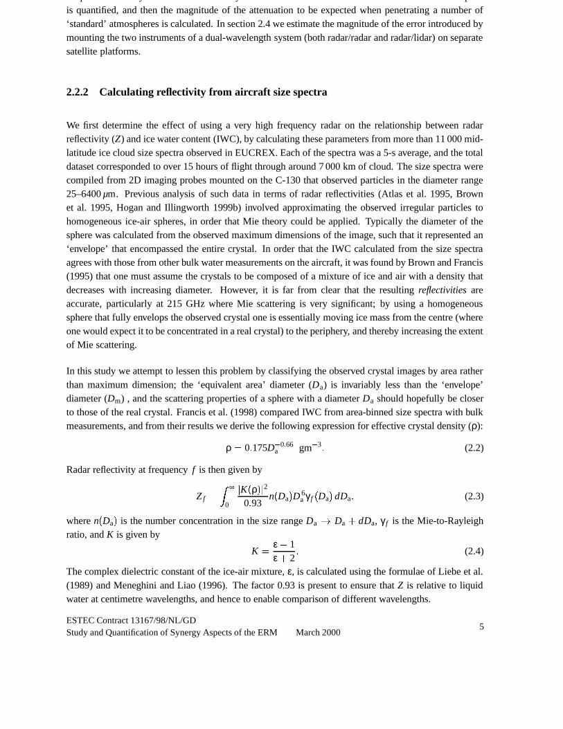
2.2.2 Calculating reflectivity from aircraft size spectra

We first determine the effect of using a very high frequency radar on the relationship between radarreflectivity (Z) and ice water content (IWC), by calculating these parameters from more than 11 000 mid-latitude ice cloud size spectra observed in EUCREX. Each of the spectra was a 5-s average, and the totaldataset corresponded to over 15 hours of flight through around 7 000 km of cloud. The size spectra werecompiled from 2D imaging probes mounted on the C-130 that observed particles in the diameter range25–6400 µm. Previous analysis of such data in terms of radar reflectivities (Atlas et al. 1995, Brownet al. 1995, Hogan and Illingworth 1999b) involved approximating the observed irregular particles tohomogeneous ice-air spheres, in order that Mie theory could be applied. Typically the diameter of thesphere was calculated from the observed maximum dimensions of the image, such that it represented an‘envelope’ that encompassed the entire crystal. In order that the IWC calculated from the size spectraagrees with those from other bulk water measurements on the aircraft, it was found by Brown and Francis(1995) that one must assume the crystals to be composed of a mixture of ice and air with a density thatdecreases with increasing diameter. However, it is far from clear that the resulting reflectivities areaccurate, particularly at 215 GHz where Mie scattering is very significant; by using a homogeneoussphere that fully envelops the observed crystal one is essentially moving ice mass from the centre (whereone would expect it to be concentrated in a real crystal) to the periphery, and thereby increasing the extentof Mie scattering.

In this study we attempt to lessen this problem by classifying the observed crystal images by area ratherthan maximum dimension; the ‘equivalent area’ diameter (Da) is invariably less than the ‘envelope’diameter (Dm) , and the scattering properties of a sphere with a diameter Da should hopefully be closerto those of the real crystal. Francis et al. (1998) compared IWC from area-binned size spectra with bulkmeasurements, and from their results we derive the following expression for effective crystal density (ρ):

ρ � 0 � 175D � 0 � 66a gm � 3 � (2.2)

Radar reflectivity at frequency f is then given by

Z f� � ∞

0 � K � ρ � �2

0 � 93n � Da � D 6

a γ f � Da � dDa � (2.3)

where n � Da � is the number concentration in the size range Da � Da � dDa, γ f is the Mie-to-Rayleighratio, and K is given by

K � ε � 1ε � 2

� (2.4)

The complex dielectric constant of the ice-air mixture, ε, is calculated using the formulae of Liebe et al.(1989) and Meneghini and Liao (1996). The factor 0.93 is present to ensure that Z is relative to liquidwater at centimetre wavelengths, and hence to enable comparison of different wavelengths.


5

−40 −30 −20 −10 0 1010

−4

10−3

10−2

10−1

100

IWC

(g

m−3

)

94 GHz radar reflectivity (dBZ)−40 −30 −20 −10 0 10

10−4

10−3

10−2

10−1

100

IWC

(g

m−3

)

215 GHz radar reflectivity (dBZ)

Figure 2.2: Scatterplots of IWC versus 94 GHz and 215 GHz radar reflectivity for the EUCREX aircraftspectra. Over 11 000 observations are present, representing around 15 hours of data in mid-latitude icecloud.

Validation of radar reflectivity calculated from aircraft size spectra have so far been rather limited. AtRayleigh-scattering frequencies we are confident that Z calculated from aircraft microphysical measure-ments is fairly accurate, since the reflectivity of a single crystal is proportional to the square of its mass,but insensitive to size of particle over which the mass is distributed. This was confirmed during the ESACloud Lidar and Radar Experiment (CLARE’98) by simultaneous measurements with the C-130 aircraftand the scanning 3 GHz radar at Chilbolton, England (see Hogan and Goddard 1999 for an example).At 94 GHz, validation is more troublesome because attenuation (predominantly by water vapour) greatlyreduces the range out to which comparison can be performed. Donovan et al. (1999) found reasonableagreement between the Z in ice cloud measured by an airborne 95 GHz radar with the values calculatedfrom in situ measurements (using both area- and Dm-binned spectra), although there were some uncer-tainties regarding the calibration of that particular radar. Hogan et al. (2000a) showed from scatteringcalculations that the assumed density could affect IWC and particle size retrievals using dual-wavelengthradar at 35 GHz and 94 GHz by as much as a factor of two. This would be no less true at 215 GHz, andfor radar/lidar retrievals, so there is clearly both more theoretical and observational work to be done.

2.2.3 Relationship between radar reflectivity and IWC

It was shown by Brown et al. (1995) that the reflectivity from a single 94 GHz radar can be used toestimate IWC with an rms error of around a factor of two. Figure 2.2 shows scatterplots of IWC againstZ at both 94 GHz and 215 GHz calculated from the area-binned EUCREX spectra. The beneficial effectof Mie scattering at 215 GHz to reduce the strong dependence of Z on size noticeably reduces the scatter,particularly for the most radiatively significant clouds with the highest values of IWC: above 0.1 g m � 3

the rms error at 215 GHz falls to � 50% and � 35% (around a factor of 1.5). Interestingly, this is the


6

0 25 50 75 1000

2

4

6

Effective Radius re (µm)

DW

R35

, 94 (

dB) 35 GHz / 94 GHz

0 20 40 60 800

2

4

6

Z35

/ IWC (mm6g−1)

DW

R35

, 94 (

dB)

0 25 50 75 1000

2

4

6

8

10

12

14

Effective Radius re (µm)

DW

R94

, 215

(dB

)

94 GHz / 215 GHz

0 10 20 30 400

2

4

6

8

10

12

14

Z94

/ IWC (mm6g−1)

DW

R94

, 215

(dB

)

Figure 2.3: Scatterplots of dual-wavelength ratio (DWR) versus effective radius and the ratio of reflectiv-ity to ice water content. The top panels are for a dual-wavelength combination of 35 GHz and 94 GHz,and the bottom panels correspond to the 94 and 215 GHz combination. The solid lines depict ‘best-fit’relationships between the various parameters and the dashed lines correspond to one standard deviationfrom the mean. These data were calculated from the area-binned EUCREX size spectra in mid-latitudeice cloud.

same value as the accuracy that Brown et al. (1995) calculated for IWC retrievals using a 94 GHz radarwhen some measure of size was available in addition to the radar reflectivity. It should be noted that iffrequencies lower than 94 GHz are used then the scatter becomes appreciably worse.


7

2.2.4 Effective radius and IWC from dual-wavelength radar

To fully constrain the radiation budget it is necessary to obtain some measure of ice crystal size, in addi-tion to IWC. The most commonly-used size parameter in clouds is effective radius (re), which followingFrancis et al. (1994) we define as

re� 3

4IWC

ρi � ∞0 n � A � A dA � (2.5)

where ρi is the density of solid ice and A is the ice crystal cross sectional area. When area-binned dataare used, A can of course be calculated exactly. Effective radius should be directly related to DWR.Additionally, we can relate DWR to the ratio between reflectivity at the longer of the two wavelengthsand IWC; in this way the combination of Z and DWR allows IWC to be measured more accurately thanis possible from Z alone.

Figure 2.3 shows scatterplots of DWR versus both re and the ratio of Z to IWC, calculated from theEUCREX data binned by area. We have used both the 35/94 GHz and 94/215 GHz frequency combina-tions, and it can be seen instantly that the sensitivity of DWR to size effects is much stronger when thehigher of the two frequencies is 215 GHz. For the 35/94 GHz combination, DWR tends not to exceed 4dB (consistent with the observations of Hogan et al. 2000a), whereas for the 94/215 GHz combinationit can attain values of 10 dB. Also shown are lines of best fit, calculated by interpolating between themean values of re and Z � IWC in unequally-spaced ranges of DWR. The dashed lines are one standarddeviation from the mean, and indicate that both IWC and re could be retrieved with an rms error of aslittle as 10–20%. These values are in broad agreement with those of Hogan and Illingworth (1999b), buttheir lines of best fit were different by up to a factor of two because they used aircraft size spectra binnedby Dm. It only after the issue of interpretation of aircraft data in terms of radar reflectivity is resolvedthat retrieval errors as low as 20% could be realised.

Dual-wavelength radar has the potential to make very useful measurements when the particles are suf-ficiently large that DWR is greater than around 1 dB, but the limitation is clearly for the small crystalsthat have a DWR only slightly greater than 0 dB. This is of particular significance for a spaceborne radarwhich must use short dwells (around 1 s) to maintain horizontal resolution, thus limiting the precision ofZ compared to ground-based systems which can integrate over several minutes if necessary. In the pro-cessing of cloud radar data, the contribution to the signal from thermal and instrumental noise is usuallysubtracted. This enables the radar to detect genuine meteorological signals that are 15 dB smaller thanthe noise signal, although the accuracy of the measurements at low signal-to-noise ratios is much worse.It can be shown (e.g. Hogan 1998) that for a radar with a noise-equivalent reflectivity for a single pulseN (in dBZ), the standard error of a reflectivity measurement averaged over M independent pulses is givenapproximately by

∆Z � 4 � 343�M

�1 � 100 � 1 � N � Z �� dB � (2.6)

It is valid to assume that all pulses of a spaceborne radar are independent, so for the radar proposedfor the ERM with a pulse repetition frequency of 5500 Hz, a 1.4-s dwell (10 km along-track averaging)corresponds to M � 7700. ESA (1999) defined a cloud to be detectable if it had a ‘radiometric resolution’of less than 1.44 dB, equivalent to setting the maximum-allowable ∆Z to 1.7 dB. Figure 2.4 shows ∆Zversus Z for a a radar with a ‘minimum detectable reflectivity’ (in the absence of attenuation) of � 36.8dBZ. This was the value calculated by ESA (1999), although their definition of Z resulted in a value 1.3


8

−40 −35 −30 −25 −20 −15 −10 −5 00

0.2

0.4

0.6

0.8

1

1.2

1.4

1.6

1.8

2

Reflectivity factor Z (dBZ)

Pre

cisi

on o

f Z (

dB)

Figure 2.4: The precision of measured radar reflectivity for 7700-pulse averaging (10 km) and a noise-equivalent reflectivity of � 22 � 2 dBZ.

dB higher. The error in DWR is given by

∆DWR �� ∆Z2l � ∆Z2

s � 1 � 2 dB � (2.7)

At large signal-to-noise ratios ∆Z � 0 � 05 dB, and so assuming the two radars are equally sensitive,∆DWR � 0 � 07 dB. For the 35/94 GHz dual-wavelength combination this corresponds to a minimum-measurable re of around 45 µm, while for the 94/215 GHz combination this puts a lower limit to themeasurable re of around 25 µm. However, in many situations where small particles are present, thereflectivity will be low, and the corresponding error in DWR could be too high for accurate size retrieval.Figure 2.5 shows the fraction of clouds for which size can be estimated as a function of Z for the twowavelength combinations 35/94 GHz and 94/215 GHz. In each case, two criteria for acceptable errorsin DWR have been considered; the solid line corresponds to DWR � ∆DWR and the dashed line isfor DWR � 2∆DWR. As expected the fraction of clouds that can be sized increases rapidly as thesignal-to-noise ratio increases. Considering the second and more stringent of the two criteria, we seethat only around 20% of clouds with a reflectivity of � 20 dBZ could be sized by a 35 GHz and 94 GHzdual-wavelength radar, but this value rises to around 85% for the 94 GHz and 215 GHz combination.

2.2.5 Attenuation at 215 GHz

We have demonstrated several advantages in using 215 GHz radar to observe ice clouds from space.The only disadvantage when compared to 94 GHz would appear to be the higher attenuation, which weshall quantify now. The nadir two-way gaseous attenuation from space has been calculated using theline-by-line model of Liebe (1985), for three standard atmospheres taken from McClatchey et al. (1972),


9

−40 −30 −20 −10 00

0.2

0.4

0.6

0.8

1


Fra

ctio

n of

clo

uds

whi

ch a

re s

ized

35 GHz / 94 GHz combination

DWR > ∆DWR DWR > 2∆DWR

−40 −30 −20 −10 00

0.2

0.4

0.6

0.8

1


Fra

ctio

n of

clo

uds

whi

ch a

re s

ized

94 GHz / 215 GHz combination

DWR > ∆DWR DWR > 2∆DWR

Figure 2.5: The fraction of detected cloud that can be sized by a dual-wavelength radar with a minimum-detectable reflectivity of � 36.8 dBZ (shown by the vertical dot-dashed line). The two panels correspondto the two wavelength combinations under consideration.

but with saturated layers added at altitudes typical of cirrus. Figure 2.6 shows the profiles of temperature,relative humidity and the corresponding two-way nadir attenuation at five different frequencies. In mid-latitude summer and the tropics it can be seen that the attenuation at 0 � C (4 km) reaches at most around0.4 dB at 94 GHz and 2 dB at 215 GHz. This is not a great problem for a 94/215 GHz dual-wavelengthsystem since the reflectivity at 215 GHz can be matched with the 94 GHz value in the Rayleigh-scatteringcloud top, and the attenuation then corrected through the remainder of the cloud assuming the relativehumidity to be 100% wherever there is a cloud echo. In any case, the crystals at the base of a thick cloudare likely to be large enough that even an error in DWR of 1 dB after attenuation correction is likely tobe significantly less than the magnitude of DWR due to Mie scattering, and the retrieved size should notbe greatly biased.

The attenuation by the ice crystals themselves also increases with frequency, but is still a much smallereffect than attenuation by water vapour. At 94 GHz it can be neglected, and at 215 GHz it has beencalculated from aircraft datasets by that only 2.1% of tropical cirrus and 0.2% of mid-latitude cirrusshould have a two-way extinction of greater than 1 dB km � 1 (Hogan and Illingworth 1999b).

Clearly 215 GHz is not a good choice of wavelength if detection of low stratocumulus is a priority; thetwo-way attenuation to the ground is around 20 dB in the case of mid-latitude summer and tropical cases.In any case, it is doubtful that the radar return from stratus and stratocumulus can be used quantitativelysince the ubiquitous presence of the occasional drizzle drop means that Z is essentially unrelated to liquidwater content (Fox and Illingworth 1997).


10

0.001 0.01 0.1 1 10 0

2

4

6

8

10

12

14

16

18

20

Two−way attenuation from space (dB)

Hei

ght (

km)

Mid−latitude winter atmosphere + cirrus

35 GHz 79 GHz 94 GHz 140 GHz215 GHz

0 20 40 60 80 100

Relative Humidity (%)−60−40−20 0 20

Temperature (°C)

0.001 0.01 0.1 1 10 0

2

4

6

8

10

12

14

16

18

20


Hei

ght (

km)

Mid−latitude summer atmosphere + cirrus


0 20 40 60 80 100


Temperature (°C)

0.001 0.01 0.1 1 10 0

2

4

6

8

10

12

14

16

18

20


Hei

ght (

km)

Tropical atmosphere + cirrus


0 20 40 60 80 100


Temperature (°C)

Figure 2.6: The two-way attenuation from space at five frequencies for three standard atmospheres withcirrus added at typical altitudes.

2.2.6 Conclusions

We have explored the feasibility of spaceborne 215 GHz radar in both single- and dual-frequency con-figurations. For a single frequency system, 215 GHz has several advantages over the more usually con-sidered frequency of 94 GHz, the principle one of which is that IWC can be more accurately estimatedfrom Z alone. At 215 GHz the error in IWC decreases from � 140%/ � 60% for IWC � 0 � 001 g m � 3 to� 50%/ � 35% for IWC � 0 � 1 g m � 3, while at 94 GHz it is somewhat higher, falling from � 200%/ � 65%for IWC � 0 � 001 g m � 3 to � 65%/ � 40% for IWC � 0 � 1 g m � 3. Additionally, the higher frequency


11

affords a greater sensitivity and a smaller footprint. This suggests that for simultaneous radar and lidarobservations of ice clouds it might be worthwhile considering 215 GHz as the radar frequency. Theattenuation at 215 GHz in ice clouds is generally small enough not to detrimentally affect the retrievals.However, if the detection of low clouds is a priority then 215 GHz is not a suitable choice for a single-wavelength system since the two-way attenuation can be as much as 20 dB in the lowest 3 km. In thenext section we attempt to quantify the lidar attenuation in real ice clouds for comparison with the 215GHz values.

Our results suggest that dual-wavelength 94/215 GHz radar has the potential measure re and IWC tobetter than 20%. The technique is most effective in the thicker, more radiatively significant clouds wherethe crystals are large enough to Mie scatter significantly at 215 GHz. It is these clouds that would be mostattenuating for the lidar, and therefore the most difficult to size using the radar/lidar method. It should benoted that the estimated accuracy of dual-wavelength radar retrievals is somewhat of a best guess; there isstill much uncertainty as to how to represent the density of ice crystal in scattering calculations. However,this is no less true of the theoretical work underlying radar/lidar retrieval algorithms. Unfortunately theproblem of boundary-layer attenuation makes it very difficult to use a real ground-based 215 GHz systemto validate retrievals techniques in ice cloud, so if such an instrument were to be considered seriously fora satellite mission, data would need to be taken by an airborne 215 GHz radar.


12

2.3 Lidar attenuation

It is interesting to compare the values of attenuation at 215 GHz with those for a spaceborne lidar. Wehave estimated the lidar attenuation from space using 2.5 months of data recorded by the vertically-pointing 94 GHz Galileo radar at Chilbolton, England, between 5 November 1998 and 24 January 1999.Radar reflectivity was converted to lidar extinction coefficient (α) using the following formula, whichwas derived as a best-fit to the EUCREX area-binned aircraft data:

log10 � α � � 0 � 546 Z94 � 2 � 7131 � (2.8)

where α has the units m � 1 and Z94 is in dBZ. The radar was carefully calibrated during the CLARE’98campaign (Hogan and Goddard 1999), but it has been necessary to add a fixed value of 2 dB to the Zvalues to very roughly account for water vapour attenuation through the boundary layer. It should benoted that there is a considerable degree of scatter in the relationship between Z and α, and also thatthese observations take no account of the presence of highly-attenuating supercooled liquid water clouds(studied later in this report), so the estimates of lidar attenuation should be regarded as rather preliminaryand if anything rather conservative. The results are shown in Fig. 2.7. The left panel shows the frequencythat the attenuation down to any pixel in the atmosphere would exceed a particular value. At a height of4 km, we see that around 25% of the pulses would be attenuated by more than 3 dB (two way), while15% would be attenuated by 10 dB or more. However, this is misleading since we are obviously onlyinterested in lidar returns when there is some cloud present. When only the attenuation down to cloudypixels is considered (right panel) the results for the spaceborne lidar are considerably worse: 73% of thereturns from cloud at 4 km would be attenuated by at least 3 dB, and 53% of them by at least 10 dB.

0 2 4 6 8 10 12 14 16 18 201

2

3

4

5

6

7

8

9

10

11

Two−way lidar attenuation from space (dB)

Hei

ght (

km)

Attenuation to any pixel

0.01

0.01

0.1

0.1

0.2

0.2

0.30.4

0 2 4 6 8 10 12 14 16 18 201

2

3

4

5

6

7

8

9

10

11

Two−way lidar attenuation from space (dB)

Hei

ght (

km)

Attenuation to cloudy pixels only

0.01

0.01

0.1

0.1

0.2

0.2

0.3

0.3

0.4

0.4

0.5

0.5

0.5

0.6

0.6

0.7

0.7

0.8

0.8

Figure 2.7: Frequency that the attenuation of the signal from a spaceborne lidar through ice cloud wouldexceed a given amount. The left plot considers the penetration down to any pixel, while the right plot con-siders only penetrations down to cloudy pixels. These values were estimated from 76 days of continuous94 GHz radar observations at Chilbolton during winter 1998/1999.


13

These results highlight a potentially very difficult problem that must be tackled if lidar and radar are tobe used quantitatively in ice clouds, particularly for the retrieval of effective crystal size. The attenuationat 215 GHz by water vapour and ice clouds appears rather small by comparison, and suggests that formany clouds dual-wavelength radar would be more effective for IWC and size retrievals than a radar andlidar.


14

2.4 Effect of instrument separation on radar/lidar and dual-wavelengthradar backscatter ratio

2.4.1 Introduction

Financial constraints may exclude the possibility of a payload of two active instruments on a cloudprofiling satellite, and the alternative currently proposed by NASA is to mount the radar and the lidaron two separate satellites in very close orbits. Since clouds can be very inhomogeneous it is importantto determine how detrimental the separation of the footprints would be on the quality of the synergeticinformation, such as cirrus effective radius. ESA estimated that a second satellite could trail the firstwith the footprints drifting towards and away from each other by as much as 5 km. NASA on the otherhand believe that the orbits and instrument pointing angles can be configured such that the lidar footprintwould nearly always lie within the wider swath of the radar.

In this section synthetic cirrus cloud fields are generated with the same spectral characteristics as thoseobserved by ground based radars. The spaceborne radar and lidar, and the 94/215 GHz dual-wavelengthradar, are ‘flown’ across the cloud fields with varying footprint separation, and the changes in the mea-sured backscatter ratio are calculated as a function of footprint separation. By comparison of these errorswith the range of values that the backscatter ratio can take with varying effective radius, we can deter-mine whether the errors due to footprint separation are manageable, or whether they are so great that the‘Split Mission’ scenario is not a viable option.

2.4.2 Generation of synthetic cloud fields

In order to estimate the magnitude of the errors arising from non co-located footprints we need to knowthe typical spatial structure of real cirrus clouds. This information has been obtained using vertically-pointing ground-based 35 GHz and 94 GHz observations at Chilbolton, England. Ten second averagesof reflectivity factor were recorded with a vertical resolution of 75 m. Vertical averaging was performedto reduce the vertical resolution to 525 m, close to the 500 m proposed for a spaceborne radar. Anumber of 1024-point time-series of reflectivity factor (in dBZ) in cirrus were selected, and the temporalscale converted to a spatial scale using a simple Taylor transformation and the mean wind speed overChilbolton at that time and altitude as diagnosed by the UK Met Office Mesoscale Model. Only time-series in which all points registered cloud were considered. Information on the horizontal structure wasthen obtained by fitting power laws of the form

E � E0 kµ (2.9)

to the Fourier spectra of these data, where k is wavenumber, E is power spectral density, and E0 and µare the coefficients. The best fit lines were least-squares fits in log-log space after 7-point averaging ofthe spectra to reduce scatter. The parameter µ was found to vary between � 1.8 and � 2.4 in cirrus, whichcompares with the range � 1 to � 2 found by Danne et al. (1996). No significant difference was foundbetween the spectra measured by the 35 GHz and 94 GHz radars. A spectrum typical of those analysedis shown in Fig. 2.8. It had the form E � 2 � 03 � 10 � 5k � 2 � 16 dBZ2 m (where k is in m � 1), and we willuse this from now on.


15

10−6

10−5

10−4

10−3

10−2

10−1

100

101

102

103

104

105

106

Wavenumber k (m−1)

Ref

lect

ivity

ene

rgy

dens

ity E

(dB

Z2 m

)

Figure 2.8: The power spectrum from 35 GHz reflectivity observations in cirrus at an altitude of 7 km.Time was converted to horizontal distance using a mean wind at this altitude of 30 m s � 1. The best fitline is E � 2 � 03 � 10 � 5k � 2 � 16 �Cloud fields were generated by calculating the inverse two-dimensional Fourier transform of syntheticmatrices containing wave amplitudes consistent with the energy at the various scales indicated by theone-dimensional spectrum. See Hogan (1998) for a more complete explanation of the procedure. Thephase of each wave component of the matrix was random, so that each cloud field was different. Thedomains were square and measured 25.6 km on a side with a resolution of 100 m. Fourier analysis ofcross-sections through the domain confirmed that they had almost identical spectral properties as theoriginal data. Note that the synthetic cloud fields are spectrally isotropic, whereas real cirrus clouds withfallstreaks are not because the fallstreaks tend to be aligned parallel to the vertical wind-shear vector. Onaverage this is not expected to significantly bias the results.

2.4.3 Simulation of dual-wavelength radar overpasses

First the effect of separation on retrievals by dual-wavelength radar at 94 GHz and 215 GHz is deter-mined, using 64 synthetic cloud fields generated using the procedure described above. The footprintsof the 94 GHz and 215 GHz radar are taken to be 700 m and 305 m respectively, and Gaussian beampatterns are used. We consider swath lengths of 1 km and 10 km, corresponding to integration timesof 0.14 s and 1.4 s respectively. It is assumed that we need only consider separations in the directionperpendicular to the direction of motion of the satellite; separations in the direction parallel to the motionof the satellites can in principle be corrected for by applying an appropriate time lag to the data from oneof the instruments. This of course assumes that the cloud does not evolve significantly in the intervening


16

94 GHz radar

215 GHz radar

25.6 km × 25.6 km × 0.5 km

−20

−15

−10dBZ

0 1 2 3 4 5 6 7 8 9 100

0.5

1

1.5

2

2.5

3

3.5

Radar separation (km)

RM

S e

rror

(dB

)

1 km integration (minimum error 0.087 dB)10 km integration (minimum error 0.039 dB)

Figure 2.9: RMS error in the dual-wavelength radar ratio as a function of footprint separation.

94 GHz radar

lidar

25.6 km × 25.6 km × 0.5 km

−20

−15

−10dBZ

0 1 2 3 4 5 6 7 8 9 100

0.5

1

1.5

2

2.5

3

3.5

Radar/lidar separation (km)

RM

S e

rror

(dB

)

1 km integration (minimum error 0.095 dB)10 km integration (minimum error 0.037 dB)

Figure 2.10: RMS error in the lidar/radar backscatter ratio as a function of footprint separation.

period.

The scenario for a 10 km integration is shown schematically in Fig. 2.9, along with the error in DWR asa function of separation, calculated from the results of flying the imaginary satellites over each of the 64different cloud fields. We see that if the two radars were mounted on the same satellite such that theirfootprints were superposed, the error in DWR due to differences in footprint size would be less than0.1 dB for both 1 km and 10 km integration. This is less than the random error due to a finite numberof pulses being averaged, and is quite acceptable for crystal size retrieval. However, when the radarsare separated by 5 km the error exceeds 2 dB, which from Fig. 2.3 we see would greatly degrade thesize information available from the two instruments, and make sizing of the smaller crystals much moredifficult. Hence for a dual-wavelength radar it would seem that there is little point in even attempting toderive size with errors of this magnitude.

2.4.4 Simulation of radar and lidar overpasses

The same synthetic cloud fields are now used to compute the effect of instrument separation on radar/lidarsynergy. The lidar footprint is assumed to be 100 m across (1 pixel of the simulated cloud field), and wefollow the specification of the ATLID instrument (ESA 1999) and assume a pulse repetition frequencyof 35 Hz, which results in each footprint being 200 m apart. The radar reflectivity field is converted to


17

lidar backscatter coefficient using the formula relating reflectivity to extinction coefficient given in (2.8),and assuming a constant extinction-to-backscatter ratio of 15 sr. It turns out that because the errors areexpressed logarithmically, the functional form of this relationship has no effect on the rms error of thebackscatter ratio. This is shown in Fig. 2.10: the error in backscatter ratio (in dB) is almost exactly thesame as for the dual-wavelength radar, except when the beams are entirely overlapped, for which theerror is very slightly larger. This is simply because the difference in footprint size is greater. As before,a separation of 5 km results in an error of over 2 dB. Because the change in radar/lidar backscatter ratiowith effective radius is much more than the change in dual-wavelength radar ratio, an error of 2 dB doesnot necessarily mean that particle sizing becomes impossible, although it is by no means insignificant.

2.4.5 Conclusions

We have examined the implications of the ‘Split Mission’ scenario on both radar/lidar and dual-wavelength radar retrievals using simulated but realistic 2D cloud fields. It is found that when theinstruments are mounted on the same platform, the rms error is less than 0.1 dB, despite the differ-ences in footprint size. If they are separated by 5 km then the error increases to more than 2 dB. Thisis unacceptable for a dual-wavelength radar. The radar/lidar technique is intrinsically more forgivingof errors (providing the lidar is corrected for attenuation) because the range over which the radar/lidarratio varies with changing effective radius is so much greater, but certainly an error of this magnituderepresents an unwelcome complication.


18

2.5 Identification of supercooled clouds using radar and lidar

2.5.1 Introduction

Of primary importance in determining the radiative properties and evolution of a cloud is its phase.Mixed-phase clouds could potentially play an important role in the climate system (Sun and Shine 1995),but due to a lack of good observational datasets there is much uncertainty regarding the extent to whichice and liquid water coexist, and how to represent the ice to liquid water ratio below 0 � C in forecast andclimate models. Intuitively one might expect microscale coexistence of the two phases to be rare sincesuch a situation is inherently unstable, with the ice crystals able to grow rapidly at the expense of theliquid water droplets by virtue of the difference in saturation vapour pressure (the ‘Begeron-Findieson’mechanism). Most models crudely assume that the ice/liquid water ratio is a function of temperaturealone, and varies smoothly from purely liquid water at 0 � C to purely ice at some lower temperature.However, this lower temperature varies significantly among parameterisations (Smith 1990, Sundqvist1993, Bower et al. 1996), and its value has been found to have a strong impact on mean cloud amount andconsequently the radiation budget (Gregory and Morris 1996, Fowler and Randall 1996). From a largeaircraft dataset, Moss and Johnson (1994) demonstrated that this lower temperature should be around

� 9 � C, but there was considerable scatter in their data, clearly suggesting that temperature alone is notsufficient to characterise the ice/liquid water ratio. Indeed there is no reason to suppose that supercooledstratocumulus, altocumulus, cumulonimbus and fronts should each have the same relationship. Morecomplex parameterisations have been proposed that make use of other model parameters such as verticalvelocity (Tremblay et al. 1996, Wilson and Ballard 1999), but it is very likely that the formation of su-percooled water (in stratiform rather than vigorously convective clouds) is subject to small-scale verticalmotions that if averaged over a model gridbox would not be sufficient to cause condensation of liquidwater. Furthermore, the rate of glaciation is very much dependent on how well the ice and liquid waterare mixed within the gridbox.

There is clearly an urgent need for observations to improve our understanding of both the importantmicrophysical processes that act in mixed-phase clouds and the resulting cloud-scale distribution of iceand liquid water. In situ aircraft measurements have been used to provide useful statistics on mixed-phase clouds, but to get an idea the overall cloud morphology requires high-resolution remote sensingtechniques that have the ability distinguish liquid water from ice.

The most well-known method for remotely inferring cloud phase is the polarisation lidar technique; non-spherical ice crystals can be distinguished from liquid water droplets because they depolarise the incidentlight (Sassen et al. 1990). Eberhard (1995) proposed the use of dual-wavelength CO2 lidar, which utilisesthe fact that the ratio of backscatter coefficient at suitably separated wavelengths is different for liquiddroplets and ice crystals. The main limitation of ground-based lidars is that they are strongly attenuatedby intervening liquid water clouds, so while they are useful for studying altocumulus (e.g. Sassen 1991,Heymsfield et al. 1991, Wylie et al. 1995), they cannot be used from the ground to study glaciatingstratocumulus or the mixed-phase regions of precipitating frontal systems. Gosset and Sauvageot (1992)suggested using the differential attenuation of a dual-wavelength radar to retrieve liquid water contentin a mixed-phase cloud, while the absolute value of radar reflectivity could be used to infer ice watercontent. However, if the wavelength of a radar is short enough for the attenuation through a cloud with


19

a potentially small liquid water content to be measurable, then it is very likely that the larger crystalsin the cloud would scatter well outside the Rayleigh regime, and radar reflectivity differences could notbe unambiguously attributed to differential attenuation. Hogan et al. (1999) showed that ice crystalsgrowing in the presence of supercooled water tend to be needles or plates with extreme aspect ratios,which can be detected by a polarisation radar as very high values of differential reflectivity. While thisis useful for microphysical studies, it relies on ice being present, and cannot be used on its own to derivereliable statistics on the occurrence of supercooled water because it is such an indirect measurement.

In this section we demonstrate that supercooled water in the atmosphere often tends to occur in the formof layers composed of high concentrations of small droplets, which give a strong echo at the lidar wave-length, while the echo at the radar wavelength tends to be dominated by the contribution from the largerice crystals so that the contribution from the supercooled layer is masked. This is demonstrated in Fig.2.11, which shows a time-height section of lidar backscatter coefficient (β) from the 905 nm VaisalaCT75K lidar ceilometer at Chilbolton (resolution 30 m and 30 s) through a typical layer with a tempera-ture of around � 20 � C. The data were taken on 15 October 1998 during the CLARE’98 field campaign.Small cells characteristic of altocumulus are apparent in the accompanying photograph from the cloudcamera, indicating that the layer is convective in nature. No layer is visible in the accompanying observa-tions by the 35 GHz Rabelais radar at Chilbolton (resolution 75 m and 30 s), since the radar echos at thisfrequency are dominated by the contribution from the larger ice particles falling beneath the glaciatingliquid water cloud. Ice cloud is visible in the photograph as much fainter but more homogeneous wispsbeneath the liquid water cells. The radiosonde ascent from Herstmonceux (125 km away) shows that thelayer was saturated with respect to liquid water and convectively unstable. The cells in the photographwere around 500 m across, too small to be resolved by the 30 s resolution of the lidar given that the windspeed at this altitude (from the radiosonde ascent) was 26 m s � 1. Heymsfield et al. (1991) presentedaircraft measurements of liquid water in two altocumulus clouds and demonstrated using a numericalmodel that the observations were consistent with radiatively-driven convective overturning.

Spaceborne lidar and radar would be ideally suited the task of detecting the presence of supercooled lay-ers on a global basis, and would have the important advantage of viewing from above and thus avoidingthe problem of extinction by low cloud. Figure 2.12 illustrates this point with observations by an air-borne 1064 nm nadir-pointing polarisation lidar in the vicinity of Chilbolton. The lidar was mounted onthe DLR Falcon aircraft, and the data were taken on 20 October 1998 during CLARE’98. A number ofstrongly-reflective layers are clearly present in the β field, and their low depolarisation indicates that theyare composed predominantly of spherical water droplets. Simultaneous measurements by the scanning 3GHz Chilbolton radar show no such features in reflectivity (Z), but do show unusually high values of dif-ferential reflectivity (ZDR), indicating the presence of horizontally-aligned, highly non-spherical crystalsfalling beneath the supercooled water layers (Hogan et al. 1999). In situ measurements by the UK MetOffice C-130 aircraft at an altitude of around 4 km ( � 7 � C) revealed the lowest elevated lidar echo to beassociated with liquid water contents of up to around 0.2 g m � 3. The vertical velocity at this altitude andmore than 25 km from Chilbolton exhibits a clear periodicity with an amplitude of around 0.6 m s � 1 anda wavelength of around 15 km, indicating that a gravity wave was probably responsible for the updraftsthat caused the supercooled liquid water to condense. From the horizontal wind speed of 18 m s � 1 wecalculate that a parcel affected by the gravity wave is vertically displaced by

�80 m, and its temperature

correspondingly varies by around�

0.6 K. The saturation vapour density would therefore vary by�

0.13g m � 3, which is very much in line with the liquid water contents observed at the crests of each wavebeyond 25 km. Lidar ceilometer observations on this day (not shown) could not penetrate the lowest of


20

09:00 10:00 11:00Time (UTC)

PhotoLidar

10−6

10−4

(sra

d m

)−1

09:00 10:00 11:00Time (UTC)

PhotoRadar

−40 −20 0

dBZ

−60 −40 −20 0 200

2

4

6

8

10

Temperature (°C)

Hei

ght (

km) lapse rate

−8.18°C/km

11:00 ascent (Herstmonceux)

15/10/98

Figure 2.11: Time-height section of lidar backscatter coefficient and 35 GHz radar reflectivity througha supercooled layer, with a simultaneous photograph from the cloud camera. The radiosonde dry-bulband dew-point temperature profile measured at Herstmonceux is also shown. The data were taken on 15October 1998 at Chilbolton.


21

−60 −50 −40 −30 −20 −10 00

0.1

0.2

Wat

er c

onte

nt (

g m

−3 )

Distance from Chilbolton (km)

C−130

LWCIWCw

−1

0

1V

ertic

al v

el. (

m s

−1 )

0

2

4

6

Hei

ght (

km)

C−130 (inbound)

3 GHz Reflectivity factor

−20

−10

0

10

20dBZ

0

2

4

6

Hei

ght (

km)

C−130 (inbound)

1064 nm Backscatter coefficient 0

2

4

6

8

10

10−6

10−4

(sr m)−1

C−130 (inbound)

3 GHz Differential reflectivity 0

2

4

6

Hei

ght (

km)

0

2

4dB

Hei

ght (

km)

C−130 (inbound)

532 nm Depolarisation ratio 0

2

4

6

8

10

0

10

20

30

40

50%

Figure 2.12: Composite of observations from the run at 1420 on 20 October 1998 during CLARE’98.The first two panels show measurements by the nadir-pointing lidar on board the Falcon aircraft flyingat an altitude of 13 km. Simultaneous measurements of Z and ZDR by the ground based 3 GHz radar atChilbolton are shown in the next two panels, and the last shows liquid water content, ice water contentand vertical velocity measured by the C-130 aircraft at an altitude of 4 km ( � 7 � C).


22

the layers at 4 km.

In the remainder of this section, several years of observations by a 905 nm Vaisala CT75K lidar ceilome-ter are analysed to estimate the frequency of occurrence of supercooled liquid water layers as a functionof temperature. It is found that they are much more common than one might suppose, highlighting theneed for further measurements on a global basis. To examine the effect of specular reflection by planarice crystals to produce layers of high β that anomalously register as supercooled water, we also examinedata from a Vaisala lidar ceilometer operating at 5 � from zenith.

2.5.2 Objective identification of layers from ceilometer data

Layers can be identified easily by eye from time-height sections of β, so the first step is to automate theprocess of layer identification using a set of fixed rules. The data acquisition system from the Vaisalainstrument outputs the height of the first cloud base (h) in addition to the β profile. It calculates h byperforming a so-called Klett inversion of the β profile assuming a fixed extinction-to-backscatter ratio,and considers the slope, absolute value and historic observations at that height. The base of liquidwater clouds (both at temperatures above and below 0 � C) are characterised by high values of β above asharp gradient in β, and comparison of h with the β profile indicates that supercooled layers identifiedsubjectively always coincide with the first cloud base. However, when no liquid water cloud is present,h is unreliable.

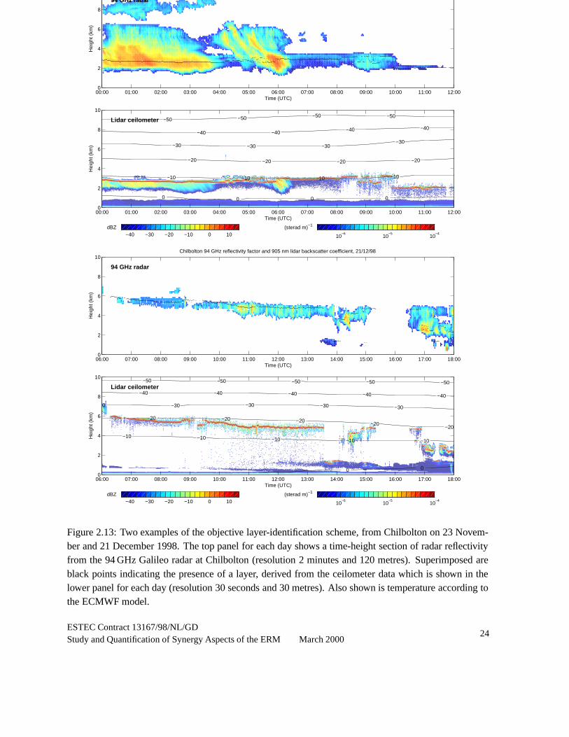
Hence we use h as the starting point for automatic layer identification, and do not attempt to identifymore than one layer in each ray. Firstly, the height of the maximum β within 150 metres of h is found.Two tests are then applied that have been found to give best agreement with layers identified subjectively:a layer of supercooled water should have a value of β greater than 4 � 10 � 5 sr � 1 m � 1 and this peak valueshould be at least 20 times greater than the value 300 m (10 range gates) above. Two examples of layeridentification using this simple algorithm are shown in Fig. 2.13. In the first case the supercooled wateroccurs at around � 8 � C and is embedded within a more extensive ice cloud. The longevity of the layerdespite the presence of ice is rather difficult to explain, and highlights the need for further case studiesinvolving in situ measurements and cloud resolving model simulations. The second case shows a moretypical altocumulus cloud topped by a layer of liquid water. In both cases the algorithm has successfullylocated the position of the layer. An algorithm based purely on the maximum value of β was tried, butit was found that very cold layers could be missed while reflective clouds that were not layer-like inappearance, such as the lower parts of deep cirrus, tended to be included.

Radiosonde data was used to estimate the temperature at the altitude of the layer. The nearest operationalupper-air station to Chilbolton is Herstmonceux, 125 km away, which carries out ascents every six hours.This station is used in preference to the so-called ‘range’ station at Larkhill, which is only 25 km awaybut does not perform regular ascents. Linear interpolation was performed in both time and height, butthere is likely to be a residual error of several degrees in the derived temperature profile over Chilbolton.


23

−40 −30 −20 −10 0 10 dBZ

10−6

10−5

10−4

(sterad m)−1

00:00 01:00 02:00 03:00 04:00 05:00 06:00 07:00 08:00 09:00 10:00 11:00 12:000

2

4

6

8

10

Hei

ght (

km)

Time (UTC)

Chilbolton 94 GHz reflectivity factor and 905 nm lidar backscatter coefficient, 23/11/98

94 GHz radar

−50 −50 −50 −50

−40 −40 −40 −40

−30 −30 −30−30

−20 −20 −20 −20

−10 −10 −10 −10

0 0 0 0

00:00 01:00 02:00 03:00 04:00 05:00 06:00 07:00 08:00 09:00 10:00 11:00 12:000

2

4

6

8

10

Hei

ght (

km)

Time (UTC)

Lidar ceilometer

−40 −30 −20 −10 0 10 dBZ

10−6

10−5

10−4

(sterad m)−1

06:00 07:00 08:00 09:00 10:00 11:00 12:00 13:00 14:00 15:00 16:00 17:00 18:000

2

4

6

8

10

Hei

ght (

km)

Time (UTC)

Chilbolton 94 GHz reflectivity factor and 905 nm lidar backscatter coefficient, 21/12/98

94 GHz radar

−50 −50 −50 −50 −50

−40 −40 −40 −40 −40

−30 −30 −30 −30 −30

−20 −20 −20 −20−20

−10 −10 −10 −10 −10

0 0

06:00 07:00 08:00 09:00 10:00 11:00 12:00 13:00 14:00 15:00 16:00 17:00 18:000

2

4

6

8

10

Hei

ght (

km)

Time (UTC)

Lidar ceilometer

Figure 2.13: Two examples of the objective layer-identification scheme, from Chilbolton on 23 Novem-ber and 21 December 1998. The top panel for each day shows a time-height section of radar reflectivityfrom the 94 GHz Galileo radar at Chilbolton (resolution 2 minutes and 120 metres). Superimposed areblack points indicating the presence of a layer, derived from the ceilometer data which is shown in thelower panel for each day (resolution 30 seconds and 30 metres). Also shown is temperature according tothe ECMWF model.


24

2.5.3 Statistics from zenith-pointing ceilometer

The algorithm has been applied to all the ceilometer data taken at Chilbolton, from when the instrumentwas installed in the summer of 1996 until April 1999. Some data is missing, particularly in the first fivemonths, but in total 2.47 million 30-second rays have been processed, equivalent to over 28 continuousmonths of observations.

We first consider the dataset as a whole to estimate the occurrence of supercooled layers as a functionof temperature. The results are summarised in Fig. 2.14. Panel (a) shows the fraction of the dataset forwhich the instrument observed any cloud in each 5 � temperature interval between � 50 � C and � 5 � C.Pixels were defined to be cloudy if the lidar backscatter coefficient was at least 2 � 10 � 7 sr � 1 m � 1.At temperatures warmer than � 5 � C the data were often contaminated by aerosol so are not shown. Amethod was devised to ‘clean-up’ the clear-air noise occasionally produced by this instrument. It canbe seen that the occurrence of cloud in each 5 � bin was less than 10% and decreased with decreasingtemperature. This will be appreciably less than the true cloud occurrence, because of the problem ofobscuration by lower level clouds at lidar wavelengths.

Panel (b) shows the fraction of clouds that contained a layer satisfying the definition given earlier, ineach 5 � interval. As one might expect, the fraction of clouds containing a supercooled layer decreaseswith temperature; 18.5% of clouds between � 10 � C and � 15 � C contained a supercooled layer, whereasbetween � 30 � C and � 35 � C the value falls to only 5.5%. The lower two panels depict similar informationbut in a cumulative sense. Panel (d) shows the fraction of observations with clouds colder than a giventemperature that contained a layer colder than this temperature. We see that around 30% of the time thatcloud colder than � 10 � C was observed, a layer was observed within it, falling to 20% when consideringonly clouds colder than � 20 � C.

Figure 2.15 shows the mean layer duration and horizontal extent as a function of temperature. Horizontalextent was calculated from layer duration using the wind speed at that height as given by the interpolatedradiosonde profile. Because of the frequent temporary obscuration of the layers by passing low levelcumulus, layers were deemed continuous in this analysis provided any gaps in them lasted no longerthan 10 minutes. We see that at � 5 � C the average layer persisted for over half an hour, with the averageduration falling steadily with decreasing temperature. Typical horizontal extents were between 20 and30 km, although because of obscuration this is likely to be a considerable underestimate. Figure 2.13shows cases in which layers were observed to persist for much longer.

An attempt was made to estimate the optical depth of these layers by performing a simple Klett-typeinversion on each profile to remove the effects of attenuation. An extinction-to-backscatter ratio suitableto liquid water of 15 sr was employed. However, all gate-by-gate procedures for correcting attenuatedbackscatter profiles are potentially unstable and very sensitive to both instrument calibration and thechosen extinction-to-backscatter ratio, and indeed our retrieved optical depths calculated by this methodwere often impossibly large. The mean optical depth of those layers for which the procedure did notexplode was around 0.2, but given the problems with this technique it is doubtful that this value isaccurate. The apparent physical thickness of the high β region was typically around 150 metres (5 rangegates), but because of the strong attenuation the true thickness is likely to be much greater.


25

−50 −40 −30 −20 −100

0.05

0.1

0.15

0.2

0.25

0.3

Temperature (°C)

Fre

quen

cy th

at c

loud

was

obs

erve

d

a

−50 −40 −30 −20 −100

0.05

0.1

0.15

0.2

0.25

0.3

Temperature (°C)

Fra

ctio

n of

clo

uds

cont

aini

ng a

laye

r

b

−50 −40 −30 −20 −100

0.05

0.1

0.15

0.2

0.25

0.3

Temperature T (°C)

Fre

quen

cy th

at c

loud

col

der

than

T o

bser

ved

c

−50 −40 −30 −20 −100

0.05

0.1

0.15

0.2

0.25

0.3

Temperature T (°C)

Fra

ctio

n of

clo

uds

with

laye

r co

lder

than

T

d

Figure 2.14: Statistics from the 31-month zenith-pointing lidar ceilometer dataset taken at Chilbolton,England: (a) Fraction of observations in which cloud was seen in each 5 � temperature range; (b) Fractionof clouds that contain a layer in each 5 � temperature range; (c) Fraction of observations in which a cloudcolder than a given temperature is observed; (d) Fraction of clouds colder than a given temperature thatcontain a layer.

We next divided the dataset into months to look for any seasonal or longer-term trend. A few months hadtoo little time in which the ceilometer was operating to produce robust statistics, so have been rejectedfrom this analysis. The remaining 31 months all have data equivalent to more than 15 continuous daysof observations, and the average is equivalent to 27.7 continuous days. Figure 2.16 shows the fraction ofclouds in three different 10 � temperature intervals that contain a supercooled layer, as a function of time.We use 10 � rather than 5 � intervals in an attempt to reduce scatter. No robust seasonal or other trend isobvious, but in any case the dataset can only really be considered continuous from February 1997, and itappears that 2 years is not sufficient to reveal any trend if one exists.


26

−50 −40 −30 −20 −100

0.1

0.2

0.3

0.4

0.5

0.6

Temperature (°C)M

ean

laye

r du

ratio

n (h

ours

)−50 −40 −30 −20 −100

5

10

15

20

25

30

Temperature (°C)

Mea

n la

yer

exte

nt (

km)

Figure 2.15: Mean duration and horizontal extent of individual layers versus temperature.

1997 1998 19990

0.1

0.2

0.3

0.4

0.5

0.6

Year

Fre

quen

cy

−5°C to −15°C

1997 1998 19990

0.1

0.2

0.3

0.4

0.5

0.6

Year

Fre

quen

cy

−15°C to −25°C

1997 1998 19990

0.1

0.2

0.3

0.4

0.5

0.6

Year

Fre

quen

cy

−25°C to −35°C

Figure 2.16: Frequency of supercooled layers in three different temperature ranges, for individualmonths.


27

It should be recognised that there is a possibility that not all layers of high β correspond to the presenceof liquid water; Thomas et al. (1990) reported observations of relatively high backscatter in ice cloud,the magnitude of which was seen to fall rapidly as the lidar pointing angle was moved a little away fromzenith. This was interpreted as being due to specular reflection from horizontally-aligned plate crystals.Throughout the period of observation by the ceilometer at Chilbolton, the instrument was operating in azenith-pointing configuration, so could be affected. This could be the reason that the fraction of cloudscontaining a layer does not fall quite to zero at � 40 � C, where because of homogeneous nucleation nosupercooled water should exist (Fig. 2.14b). Visual examination of the ceilometer data on such occasionssuggests these events are aircraft contrails, which due to the large numbers of aerosols present tend toconsist of high concentrations of very small ice crystals, so can understandably be mistaken for layersof liquid water. Indeed, Fig. 2.15 indicates that clouds identified as supercooled layers that are colderthan � 40 � C persist on average for only three minutes. It is also possible that the temperature calculatedby interpolating radiosonde profiles could be in error by in excess of 5 � . In any case, layers colderthan � 40 � C were diagnosed for only 4.9 hours of the 28 months of observations, corresponding to only0.024% of the dataset. In the next section we apply the algorithm to data from a ceilometer operating afew degrees from zenith to eliminate the effect of specular reflection.

It would seem fairly safe to assume that the layers observed by the airborne lidar in Fig. 2.12 werecomposed primarily of liquid water droplets because of the low lidar depolarisation and the in situ veri-fication. The radiosonde profile in Fig. 2.11 strongly suggests that the layer in this example is composedof liquid water. One striking property of these layers is that they tend to completely extinguish the lidarsignal (see Fig. 2.13 for an example), whereas specular reflection from plates is only an enhancement ofthe backscatter, and the extinction should remain largely unchanged. Certainly the clouds observed byThomas et al. (1990) did not strongly attenuate the lidar signal, although unfortunately absolute valuesof β were not quoted. An apparent layer was observed on 21 October 1998 during CLARE’98 at a tem-perature of around � 20 � C that had a high depolarisation ratio (indicating ice crystals) and according tothe in situ measurements did not contain significant liquid water.

2.5.4 Statistics from a ceilometer operating at 5 � from zenith

To test whether specular reflection could be affecting the results, 51 days of data from a Vaisala lidarceilometer operating 5 � from zenith at Cabau, The Netherlands have been analysed in exactly the sameway as the Chilbolton data. The observations were taken between 18 August and 4 November 1999, andradiosonde ascents from De Bilt (25 km to the north east of Cabau) were used. The results are shownin Fig. 2.17, and we see that this time only a tiny fraction of clouds colder than � 35 � C contained alayer, and the occurrence of layers is somewhat less than at Chilbolton for all temperature ranges. Thissuggests that some of the layers observed in the 31 months of zenith-pointing actually corresponded tospecular reflection from ice crystals, particularly at very cold temperatures. However, 51 days are notreally sufficient for sound statistics on supercooled layer occurrence, and several years of observationsby an off-zenith lidar would be required to confirm these findings.


28

−50 −40 −30 −20 −100

0.05

0.1

0.15

0.2

0.25

0.3

Temperature (°C)

Fre

quen

cy th

at c

loud

was

obs

erve

d

a

−50 −40 −30 −20 −100

0.05

0.1

0.15

0.2

0.25

0.3

Temperature (°C)

Fra

ctio

n of

clo

uds

cont

aini

ng a

laye

r

b

−50 −40 −30 −20 −100

0.05

0.1

0.15

0.2

0.25

0.3

Temperature T (°C)

Fre

quen

cy th

at c

loud

col

der

than

T o

bser

ved

c

−50 −40 −30 −20 −100

0.05

0.1

0.15

0.2

0.25

0.3

Temperature T (°C)

Fra

ctio

n of

clo

uds

with

laye

r co

lder

than

T

d

Figure 2.17: Statistics from 51 days of data taken by the off-zenith lidar ceilometer at Cabau, TheNetherlands: (a) Fraction of observations in which cloud was seen in each 5 � temperature range; (b)Fraction of clouds that contain a layer in each 5 � temperature range; (c) Fraction of observations inwhich a cloud colder than a given temperature is observed; (d) Fraction of clouds colder than a giventemperature that contain a layer.

2.5.5 Conclusions and future work

Lidar ceilometer data has been analysed in a first attempt to characterise the frequency of supercooledlayer clouds as a function of temperature. From a 31-month dataset it is found that they occur surprisinglyoften; 30% of the time that the lidar sees cloud colder than � 10 � C it also sees a layer colder than this.Given that they are much more radiatively important than any ice at the same altitude, and their rolein glaciation and precipitation processes, it is important that some attempt is made to represent themproperly in forecast and climate models. It would appear that a simple fixed ratio between ice and liquidwater as a function of temperature is too crude if the radiative properties of sub-freezing clouds are to be


29

simulated accurately.

Analysis of a much shorter dataset measured by a lidar ceilometer operating at a few degrees from zenithsuggested that the few layers that were observed at temperatures below � 35 � C in fact correspondedto specular reflection from the crystals in purely ice clouds. Longer periods of observation with anoff-zenith lidar are clearly required to derive robust statistics on the occurrence of supercooled layerswhile avoiding contamination of the data by specular reflection. Even the 31-month dataset was notlong enough for any seasonal or interannual trends to be evident, so it would be interesting to repeatthe procedure for even longer periods and at a number of different sites. It would also be useful toinvestigate whether the occurrence of supercooled layers can be correlated with any large scale modelfield that could be used as the basis for a parameterisation. Clearly the proposed spaceborne lidar couldplay a crucial role in gathering data on supercooled clouds on a global basis, and much would be learnedby combining β with simultaneous measurements of radar reflectivity and lidar depolarisation.


30

2.6 Deriving cloud overlap statistics from radar

2.6.1 Introduction

The distribution of clouds in the atmosphere represents one of the major uncertainties in our understand-ing of the present climate (IPCC 1995), and limits our confidence in future climate prediction. GeneralCirculation Models (GCMs) currently carry a value for cloud fraction in each model gridbox but it hasbeen found that different assumptions on the way clouds overlap in a vertical column of gridboxes canhave a strong effect on the model radiation budget (Morcrette and Fouquart 1986, Charnock et al. 1994,Liang and Wang 1997, Stubenrauch et al. 1997). This in turn affects circulation patterns (Liou and Zheng1984, Slingo and Slingo 1988, Randall et al. 1989). The three different cloud overlap assumptions thathave commonly been made in GCMs are shown schematically in Fig. 2.18. Integrations of the EuropeanCentre for Medium-Range Weather Forecasts (ECMWF) model by Morcrette and Jakob (2000) high-lighted the important differences between them: simulated global-mean cloud cover was 71.4% whenrandom overlap was assumed but only 60.9% in the case of maximum overlap, and over parts of theITCZ the resulting differences in mean outgoing longwave radiation were in excess of 40 W m � 2. Whilethe importance of cloud overlap for radiation has long been recognised, it is only recently that its role indetermining the efficiency of precipitation formation has also been studied (Jakob and Klein 1999).

Nearly all GCMs now employ the so-called ‘maximum-random’ overlap assumption, whereby verticallycontinuous clouds are assumed to be maximally overlapped while clouds at different heights that areseparated by an entirely cloud-free model level are randomly overlapped (Geleyn and Hollingsworth1979). The passive observational data used to support this approach has so far been very limited invertical resolution (Tian and Curry 1989). Barker et al. (1999) carried out Monte Carlo simulations of

Cloud cover

Hei

ght (

km)

Maximum overlap

0 0.2 0.4 0.6 0.8 10

2

4

6

8

10

Cloud cover

Hei

ght (

km)

Random overlap

0 0.2 0.4 0.6 0.8 10

2

4

6

8

10

Cloud cover

Hei

ght (

km)

Maximum−random overlap

0 0.2 0.4 0.6 0.8 10

2

4

6

8

10

Figure 2.18: A schematic illustrating the three overlap assumptions that are commonly made in GCMs.The dotted vertical lines denote total cloud cover. For clarity we have adopted the convention used byMorcrette and Jakob (2000) and drawn only a single cloud at each level. While the total cloud coverfrom the top of the atmosphere down to any particular level is correct, the use of a single cloud at eachlevel in the diagram is a simplification for the overlap of any two individual layers in the cases of randomand maximum-random overlap.


31

solar fluxes on convective clouds generated with a cloud-resolving model, and found that the overlap ofthe model clouds differed from the generally-assumed maximum-random overlap, resulting in shortwaveflux differences of up to 100 W m � 2. They looked forward to a time when overlap could be validatedfrom ground-based and spaceborne radars.

The potential of ground-based high vertical resolution radars for the validation of model cloud occurrencewas first demonstrated by Mace et al. (1998), and more recently the actual values of cloud fraction inECMWF model gridboxes were validated using radar (Illingworth et al. 1999, Hogan et al. 2000b). Itwas found that the ECMWF model exhibited a good degree of skill in predicting cloud fraction; Fig.2.19 shows a comparison of cloud fraction from the model and the observations for a ten-day period.In this section we report new results on cloud overlap derived using the same dataset as was used byHogan et al. (2000b). In contrast to the findings for cloud fraction, it is found that true cloud overlap isnot well represented by the ubiquitous maximum-random assumption, a result which could have seriousimplications for the radiation budgets of the models that use it. The technique we describe would bean ideal application for the proposed spaceborne radar, and would allow the overlap characteristics ofclouds to be measured globally.

2.6.2 Method

We use the near-continuous observations taken between 6 November 1998 and 24 January 1999 by theESTEC 94-GHz ‘Galileo’ radar at Chilbolton, England. The radar was vertically-pointing and recordedradar reflectivity factor (Z) as a 10-s average with a vertical resolution of 60 m. A 6.9 dB increasein sensitivity was achieved by averaging over 2 mins and 120 m, resulting in minimum-detectable Z ofaround � 52.5 dBZ at 1 km and � 32.5 dBZ at 10 km. The clouds most likely to be undetected by radar arehigh thin cirrus, but it was shown by Brown et al. (1995) that virtually all ‘radiatively-significant’ cirrus(essentially that which decreases outgoing longwave radiation by at least 10 W m � 2) should be detectedby a radar with a minimum-detectable Z of � 30 dBZ. A reduction in the sensitivity of the instrumentby 5 dB is found to have a negligible effect on the final results, so there is no reason to suppose thatvery tenuous clouds should have significantly different overlap characteristics from detectable clouds.Nonetheless, we restrict our analysis to data recorded below 10.5 km. Data below 750 m are not usedbecause here the radar sensitivity is somewhat compromised by leakage of the transmit pulse into thereceiver. It should be noted that the common problem of data contamination by insects is entirely absentat the latitude of Chilbolton during winter.

To compute actual overlap, daily time-height sections of Z were divided into equally-sized boxes, andwithin each box a simple ‘cloud cover mask’ was generated consisting of ‘bits’ stating whether or notcloud was present at any height within the box in each 2-minute period. To mimic the range of verticaland horizontal resolutions of current GCMs, box sizes of 360 m, 720 m, 1080 m and 1440 m in thevertical and 20 mins, 1 hour and 3 hours in time were used. Taking the mean tropospheric horizontalwind speed to be 20 m s � 1 (estimated from ECMWF model data over Chilbolton during the experimen-tal period), these temporal resolutions translate to horizontal distances of 24 km, 72 km and 216 kmrespectively, spanning the range of horizontal resolutions used by operation mesoscale models to climatemodels. Cloud cover (c) was then defined as the fraction of bits in each box that were cloudy. An ex-ample of the generation of the cloud cover mask from a 12-hour time-height section of Z is shown in


32

Hei

ght (

km) ECMWF

19 Dec 20 Dec 21 Dec 22 Dec 23 Dec 24 Dec 25 Dec 26 Dec 27 Dec 28 Dec02468

1012

Hei

ght (

km) Observations

02468

1012

0.02

0.2

0.4

0.6

0.8

0.98

Cloudfraction

Figure 2.19: Comparison of observed and ECMWF model cloud fraction at Chilbolton for a ten-dayperiod in 1998.

Fig. 2.20. It might initially appear that a vertical column of gridboxes with 100% cloud cover at everylevel is indicative of maximum overlap, but in fact nothing can be inferred about overlap when one ormore of the levels under consideration is completely cloudy, since all overlap assumptions must predictthe same total cloud cover: 100%. From the vertically continuous cloud enclosed by the red box be-tween 18 and 19 UTC, it can be seen immediately that as levels further and further apart are considered,maximum overlap becomes an increasingly poor assumption.

In order to quantify this effect, levels were analysed in pairs, with every possible combination of levelsbeing considered, and no ‘double-counting’. For each pair, four possible values for the combined cloudcover (C) of the two levels were calculated. The first was the combined cloud cover obtained assumingrandom overlap, using the standard definition

Crand� ca � cb � cacb (2.10)

(where ca and cb are the cloud covers of the lower and upper levels respectively), the second was thevalue obtained assuming maximum overlap, defined as

Cmax� max � ca � cb � � (2.11)

the third was the value obtained assuming minimum overlap, defined as

Cmin� min � 1 � ca � cb � � (2.12)

and the fourth was the combined cloud cover that was actually observed, Ctrue. Note that the subscript‘max’ corresponds to the maximum overlap and not the maximum possible C; in fact Cmax is the minimumpossible value of C (see Fig. 2.18). Pairs in which either of the levels had a cloud cover of zero or unitywere rejected, as in these cases all values of C are equal. Hence after averaging over a sufficientlylarge number of events, the position of the observed C̄true between C̄max and C̄rand (as a function of levelseparation) will tell us precisely how a radiation scheme ought to weight cloud overlap between the twoextremes of maximum and random.

A problem to consider when deriving overlap at 94 GHz is attenuation by liquid water; when heavyrain is present at low levels the radar beam can be completely obscured, resulting in vertical swaths ofapparently cloud-free air directly above the rain. This has the effect of increasing the apparent overlapsince the erroneously cloud-free regions are stacked on top of each other. We therefore use measurementstaken by a drop-counting rain gauge at Chilbolton to reject from the analysis all events for which the rain


33

Time (UTC)

Hei

ght (

km)

94 GHz radar reflectivity factor

12 13 14 15 16 17 18 19 20 21 22 23 240

2

4

6

8

10

12

−40

−30

−20

−10

0

10dBZ

Time (UTC)

Cloud cover mask

Hei

ght (

km)

12 13 14 15 16 17 18 19 20 21 22 23 240

2

4

6

8

10

12

No cloud

Cloud

Figure 2.20: An example of cloud radar data used to derive the cloud cover mask, from 11 December1998. Intermittent light drizzle was measured at the ground between 17 and 19 UTC. The resolution ofthe grid is 360 m and 1 hour.

rate exceeded 0.5 mm hr � 1 at any time during the sample period. The effect on the derived overlapcharacteristics was small because less than 10% of the data were removed in this way. The effect ofdrizzle falling beneath liquid water clouds was investigated by restricting the analysis to regions wherethe temperature was below 0 � C: the change in the overlap statistics was negligible. Another possibilityis that large but radiatively-unimportant snow crystals falling beneath ice clouds could be detected by theradar and bias the results. Analysis of simultaneous radar and lidar returns from ice clouds at all heightsby Hogan and Illingworth (1999a) revealed that this is a rare occurrence; in 94% of their data the radarand lidar cloud base agreed to within 360 m (the highest vertical resolution considered in the presentstudy).

2.6.3 Results

The results for boxes measuring 360 m by 1 hour are shown in Fig. 2.21. Pairs of levels have beengrouped together according to their vertical separation, but separated according to whether they are ver-tically continuous (i.e. the cloud cover in every interstitial level is greater than zero) or non-continuous.We see that in the case of vertically continuous cloud, as the level separation is increased from 360 m


34

0 0.2 0.4 0.6 0.8 10

2

4

6

8

10

Mean combined cloud cover

Leve

l sep

arat

ion

∆z (

km)

Vertically continuous cloud

random overlap maximum overlap mininimum overlapobserved

0 0.2 0.4 0.6 0.8 10

2

4

6

8

10

Mean combined cloud cover

Leve

l sep

arat

ion

∆z (

km)

Vertically non−continuous cloud

Figure 2.21: The mean observed combined cloud cover of pairs of levels as a function of level separation(solid line), together with the values calculated using three different overlap assumptions. The verticalresolution was 360 m and the temporal resolution was 1 hour. Only events where the cloud cover at bothlevels was greater than zero and less than one were used. The left panel was compiled from events forwhich every intermediate level contained some cloud and the right panel corresponds to cases for whichat least one of the intermediate levels was entirely cloud-free.

−0.2 0 0.2 0.4 0.6 0.8 10

2

4

6

8

10

Overlap parameter α

Leve

l sep

arat

ion

∆z (

km)


rand

om o

verla

p

max

imum

ove

rlap

Observations exp(−∆z/1.6km)

−0.2 0 0.2 0.4 0.6 0.8 10

2

4

6

8

10


Leve

l sep

arat

ion

∆z (

km)


rand

om o

verla

p

max

imum

ove

rlap

Figure 2.22: The overlap parameter α versus level separation for vertically continuous and non-continuous cloud, using boxes 360 m in height and 1 hour in duration. A value of unity indicatesmaximum overlap and a value of zero indicates random overlap.

to 4 km, C̄true moves from a value close to that calculated assuming maximum overlap, to essentially therandom overlap value. This contrasts with most current GCMs which apply maximum overlap to all ver-tically continuous levels. In the case of vertically non-continuous cloud on the other hand, there appearsto be no significant deviation of C̄true from that predicted assuming random overlap, in agreement withthe schemes used in most GCMs. Of course in individual cases Ctrue takes values anywhere between theextremes of Cmax and Cmin.

A simpler and more useful way of presenting these findings is in terms of an ‘overlap parameter’ α that


35

Temporal resolutionVertical resolution 20 mins 1 hour 3 hours

360 m 1.40 km 1.60 km 2.04 km720 m 1.68 km 1.90 km 2.30 km

1080 m 2.04 km 2.15 km 2.48 km1440 m 2.54 km 2.56 km 2.93 km

Table 2.1: Values of the e-folding distance ∆z0 for different vertical and temporal resolutions.

−0.2 0 0.2 0.4 0.6 0.8 10

2

4

6

8

10


Leve

l sep

arat

ion

∆z (

km)


rand

om o

verla

p

max

imum

ove

rlap

Observations exp(−∆z/2.04km)

−0.2 0 0.2 0.4 0.6 0.8 10

2

4

6

8

10


Leve

l sep

arat

ion

∆z (

km)


rand

om o

verla

p

max

imum

ove

rlap

Figure 2.23: The overlap parameter α versus level separation for vertically continuous and non-continuous cloud, using boxes 360 m in height and 3 hour in duration.

expresses C̄true in terms of C̄max and C̄rand:

C̄true� αC̄max � � 1 � α � C̄rand � (2.13)

Hence α � 0 corresponds to random overlap and α � 1 to maximum overlap. Figure 2.22 depicts α asa function of level separation, again for 360 m and 1 hour resolution. The observed values of α wouldseem to be best fitted by an inverse-exponential of the form

α � exp

��

∆z∆z0 � � (2.14)

where ∆z is the level separation and ∆z0 is an e-folding or ‘decorrelation’ distance. The value of ∆z0

has been estimated for each of the three temporal resolutions and four vertical resolutions by performinga least-squares fit to the observations, but weighting each observation by the number of events fromwhich the average was calculated. The results are shown in Table 2.1. Hence if cloud overlap were tobe parameterised in models using Eq. 2.14 then the value of ∆z0 could be chosen to match the modelresolution. The weighting is necessary because cloud frequency obviously decreases with increasingphysical thickness, and some possible statistical noise is apparent in α for level separations of more than7 km. Nonetheless, it is remarkable that as little as a few days of data are sufficient to exhibit essentiallythe same overlap behaviour as shown in Fig. 2.22, indicating that this 71 day dataset is easily long enoughto derive robust values of ∆z0.

It can be seen from Table 2.1 that a decrease in either temporal or vertical resolution results in an increasein ∆z0 and thus an increase in the degree of overlap for a given level separation. The change with temporal


36

resolution can be explained by considering an isolated cloud; as the box becomes larger the cloud willoccupy a decreasing fraction of the box and the apparent degree of overlap must increase. Indeed,the degree of overlap can never decrease with decreasing temporal resolution. A reduction in verticalresolution can, in individual cases, result in either an increase or a decrease in the degree of overlap, butit simply turns out that the former is more common, particularly for adjacent levels. It is found that ∆z0

does not have a significant dependence on whether the pairs of levels are taken from the upper or lowertroposphere. One interesting finding is that with a temporal resolution of 3 hours and a level separationof between 6 and 8 km, α falls to � 0.1, indicating a tendency for a lower degree of overlap than even thatpredicted by the random overlap assumption. This is shown in Fig. 2.23. The reason for this behaviouris that in Southern England during winter, fronts are almost entirely responsible for clouds more than 5km thick, and these have a characteristic ‘slanted’ signature in radar time-height sections that can onlyreally be detected in sections of 3 hours or longer. Fig. 2.20 is a striking example of such an event.

2.6.4 Conclusions

A simple method for using long-term radar observations to characterise cloud overlap has been developedthat expresses mean overlap in a way that could be implemented in GCMs. It has been found that themean overlap of vertically continuous clouds is distinctly more random than models usually assume, andthis will probably have a significant effect on the predictions made with such models. Before applyingthe findings of this study to global models it would be advisable to use the technique to derive overlapstatistics from cloud radars in other locations, and in all seasons, since the overlap characteristics ofconvective clouds may be appreciably different from those of frontal clouds. A spaceborne cloud radarwould be ideally suited to this task, and simultaneous measurements by the lidar would also be valuablein ensuring that all radiatively significant cloud is detected.


37

References

Ansmann, A., U. Wandinger, M. Riebesell, C. Weitkamp and W. Michaelis, 1992: Independent measure-ment of extinction and backscatter profiles in cirrus clouds by using a combined Raman elastic-backscatter lidar. Appl. Optics, 33, 7113–7131.

Atlas, D., S. Y. Matrosov, A. J. Heymsfield, M.-D. Chou and D. B. Wolff, 1995: Radar and radiationproperties of ice clouds. J. Appl. Meteor., 34(11), 2329–2345.

Auer, A. H., and D. L. Veal, 1970: The dimension of ice crystals in natural clouds. J. Atmos. Sci., 27,919–926.

Barker, H. W., G. L. Stephens and Q. Fu, 1999: The sensitivity of domain-averaged solar fluxes to as-sumptions about cloud geometry. Quart. J. Roy. Meteor. Soc., 125, 2127–2152.

Bower, K. N., S. J. Moss, D. W. Johnson, T. W. Choularton, J. Latham, P. R. A. Brown, A. M. Blyth andJ. Cardwell, 1996: A parametrization of the ice water content observed in frontal and convectiveclouds. Quart. J. Roy. Meteor. Soc., 122, 1815–1844.

Brown, P. R. A., and P. N. Francis, 1995: Improved measurements of the ice water content in cirrus usinga total-water probe. J. Atmos. Oceanic Technol., 12(2), 410–414.

Brown, P. R. A., A. J. Illingworth, A. J. Heymsfield, G. M. McFarquhar, K. A. Browning and M. Gosset,1995: The role of spaceborne millimeter-wave radar in the global monitoring of ice-cloud. J. Appl.Meteor., 34(11), 2346–2366.

Charnock, T., F. Rose, T. Alberta, G. L. Smith, D. Rutan, N. Manalo-Smith, P. Minnis and B. Wielicki,1994: Cloud profiling radar requirements: Perspective from retrievals of the surface and atmosphericradiation budget and studies if atmospheric energetics. In Utility and feasibility of a cloud profilingradar. Report of the GEWEX Tropical Workshop, 2–29 July 1993, Pasadena, California, IGPO 10,pp. B10–B21.

Danne, O., G. G. Mace, E. E. Clothiaux, X. Dong, T. P. Ackerman and M. Quante, 1996: Observingstructures and vertical motions within stratiform clouds using a vertical pointing 94-GHz cloudradar. Beitr. Phys. Atmosph., 69(1), 229–237.

Donovan, D. P., and A. C. A. P. van Lammeren, 2000: Combined lidar and radar cloud particle effectivesize retrievals made during CLARA. Phys. Chem. Earth, 25(2), 115–120.

Donovan, D. P., A. C. A. P. van Lammeren, R. J. Hogan, P. N. Francis, J. Testud, J. Pelon, M. Quanteand J. W. F. Goddard, 1999: Comparison of lidar/radar ice cloud parameter retrievals with in-situmeasurements. CLARE’98 Final workshop, 13–14 September 1999, ESA/ESTEC, Noordwijk, TheNetherlands, 173–177.

Eberhard, W. L., 1995: Theory for dual-wavelength CO2 lidar method to distinguish ice, mixed-phase,and water clouds. J. Atmos. Oceanic Technol., 12, 130–140.

European Space Agency (ESA), 1999: Earth Radiation Mission. ESA SP-1233 (3)—The four candidateEarth Explorer Core Missions, ESA/ESTEC, Noordwijk, The Netherlands.

Fowler, L. D., and Randall, D. A., 1996: Liquid and ice cloud microphysics in the CSU general circula-tion model. 3. Sensitivity to modeling assumptions. J. Climate, 9, 561-586.

Fox, N. I., and A. J. Illingworth, 1997: The potential of a spaceborne radar for the detection of stratocu-mulus clouds. J. Appl. Meteor., 36(6), 676–687.

Francis, P. N., A. Jones, R. W. Saunders, K. P. Shine, A. Slingo and Z. Sun, 1994: An observational and


54

theoretical study of the radiative properties of cirrus: Some results from ICE ’89. Quart. J. Roy.Meteor. Soc., 120, 809–848.

Francis, P. N., P. Hignett and A. Macke, 1998: The retrieval of cirrus cloud properties from aircraftmulti-spectral reflectance measurements during EUCREX ’93. Quart. J. Roy. Meteor. Soc., 124,1273–1291.

Geleyn, J. F., and A. Hollingsworth, 1979: An economical analytical method for the computation of theinteraction between scattering and line absorption of radiation. Contrib. Atmos. Phys., 52, 1–16.

Gosset, M., and H. Sauvageot, 1992: A dual-wavelength radar method for ice-water characterization inmixed-phase clouds. J. Atmos. Oceanic Technol., 9, 538–547.

Gregory, D., and D. Morris, 1996: The sensitivity of climate simulations to the specification of mixedphase clouds. Climate Dynamics, 12, 641–651.

Heymsfield, A. J., L. M. Miloshevich, A. Slingo, K. Sassen and D. O’C. Starr, 1991: An observationaland theoretical study of highly supercooled altocumulus. J. Atmos. Sci., 48(7), 923–945.

Hogan, R. J., 1998: Dual-wavelength radar studies of clouds. PhD Thesis, University of Reading, UK.

Hogan, R. J., and J. W. F. Goddard, 1999: Calibration of the ground-based radars used in CLARE’98.CLARE’98 Final workshop, 13–14 September 1999, ESA/ESTEC, Noordwijk, The Netherlands,63–67.

Hogan, R. J., and A. J. Illingworth, 1999a: Analysis of radar and lidar returns from clouds: Implicationsfor the proposed Earth Radiation Mission. CLARE’98 Final workshop, 13–14 September 1999,ESA/ESTEC, Noordwijk, The Netherlands, 75–80.

Hogan, R. J., and A. J. Illingworth, 1999b: The potential of spaceborne dual-wavelength radar to makeglobal measurements of cirrus clouds. J. Atmos. Oceanic Technol., 16(5), 518–531.

Hogan, R. J., A. J. Illingworth and P. R. Field, 1999: Polarimetric radar observations of the growth ofhighly-aligned ice crystals in the presence of supercooled water. CLARE’98 Final workshop, 13–14September 1999, ESA/ESTEC, Noordwijk, The Netherlands.

Hogan, R. J., A. J. Illingworth and H. Sauvageot, 2000a: Measuring crystal size in cirrus using 35- and94-GHz radars. J. Atmos. Oceanic Technol., 17(1), 27–37.

Hogan, R. J., C. Jakob and A. J. Illingworth, 2000b: Comparison of ECMWF cloud fraction with radarderived values. J. Appl. Meteor., in press.

Illingworth, A. J., R. J. Hogan and J. W. F. Goddard, 1999: Study and measurement of cloud character-istics. Final report, ESTEC Contract 10568/93/NL/NB.

Intrieri, J. M., G. L. Stephens, W. L. Eberhart and T. Uttal, 1993: A method for determining cirrus cloudparticle sizes using lidar and radar backscatter techniques. J. Appl. Meteor., 32(6), 1074–1082.

Jakob, C., and S. A. Klein, 1999: The role of vertically varying cloud fraction in the parametrization ofmicrophysical processes in the ECMWF model. Quart. J. Roy. Meteor. Soc., 125, 941–965.

Liang, X.-Z., and W. C. Wang, 1997: Cloud overlap effects on general circulation model simulations. J.Geophys. Res., 102, 11 039–11 047.

Liao, L., and K. Sassen, 1994: Investigation of relationships between Kα-band radar reflectivity and iceand liquid water content. Atmos. Res., 34, 299–313.

Liebe, H. J., 1985: An updated model for millimeter-wave propagation in moist air. Radio Science, 20(5),1069–1089.


55

Liebe, H. J., T. Manabe and G. A. Hufford, 1989: Millimeter-wave attenuation and delay rates due tofog/cloud conditions. IEEE AP, 37, 1617–1623.

Liou, K.-N., and Q. Zheng, 1984: A numerical experiment on the interactions of radiation, clouds anddynamical processes in a general circulation model. J. Atmos. Sci., 41, 1513–1535.

Liu, C.-L. and A. J. Illingworth, 2000: Towards more accurate retrievals of ice water content from radarmeasurement of clouds. Accepted J. Appl. Meteorol.

Mace, G. G., C. Jakob and K. P. Moran, 1998: Validation of hydrometeor occurrence predicted by theECMWF using millimeter wave radar data. Geophys. Res. Let., 25(10), 1645–1648.

Macke, A., J. Mueller and E. Raschke, 1993: Scattering of light by polyhedral ice crystals. Appl. Opt.,32, 2780–2788.

Matrosov, S. Y., 1993: Possibilities of cirrus particle sizing from dual-frequency radar measurements. J.Geophys. Res., 98(D11), 20 675–20 683.

Matrosov, S. Y., 1997: Variability of microphysical parameters in high-altitude ice clouds: Results of theremote sensing method. J. Appl. Meteor., 36(6), 633–648.

McClatchey, R. A., R. W. Fenn, J. E. A. Selby, F. E. Volz and J. S. Garing, 1972: Optical properties ofthe atmosphere (3rd. ed.), Air Force Cambridge Research Laboratories, Rep. No. AFCRL72-0497,L. G. Hanscom Field.

Mead, J. B., R. E. McIntosh, D. Vandemark and C. T. Swift, 1989: Remote sensing of clouds and fogwith a 1.4-mm radar. J. Atmos. Oceanic Technol., 6, 1090–1097.

Meneghini, R., and L. Liao, 1996: Comparisons of cross-sections for melting hydrometeors as derivedfrom dielectric mixing formulas and a numerical-method. J. Appl. Meteor., 35(10), 1658–1670.

Morcrette, J. J., and Y. Fouquart, 1986: The overlapping of cloud layers in shortwave radiation parame-terization. J. Atmos. Sci., 43, 321–328.

Morcrette, J.-J., and C. Jakob, 2000: The response of the ECMWF model to changes in cloud overlapassumption. Mon. Weath. Rev., 128(6), 1707–1732.

Moss, S. J., and D. W. Johnson, 1994: Aircraft measurements to validate and improve numerical modelparametrizations of ice to water ratio in cloud. Atmos. Res., 34, 1–25.

Randall, D. A., Harshvardhan, D. A. Dazlich and T. G. Corsetti, 1989: Interactions among radiation,convection and large-scale dynamics in a general-circulation model. J. Atmos. Sci., 46(13), 1943–1970.

Sassen, K., 1991: Aircraft-produced ice particles in a highly supercooled altocumulus cloud. J. Appl.Meteor., 30(6), 765–775.

Sassen, K., C. J. Grund, J. D. Spinhirne, M. M. Hardesty and J. M. Alvarez, 1990: The 27–28 Ocober1986 FIRE IFO Case Study: A five lidar overview of cloud structure and evolution. Mon. Weath.Rev., 118, 2288–2311.

Sekelsky S. M., W. L. Ecklund, J. M. Firda, K. S. Gage and R. E. McIntosh, 1999: Particle size estimationin ice-phase clouds using multifrequency radar reflectivity measurements at 95, 33 and 2.8 GHz. J.Appl. Meteor., 38(1), 5–28.

Slingo, A., and J. M. Slingo, 1988: The response of a general circulation model to cloud long-waveradiative forcing. I: Introduction and initial experiments. Quart. J. Roy. Meteor. Soc., 114, 1027–1062.


56

Smith, R. N. B., 1990: A scheme for predicting layer clouds and their water content in a general circula-tion model. Quart. J. Roy. Meteor. Soc., 116, 435–460.

Stubenrauch, C. J., A. D. DelGenio and W. B. Rossow, 1997: Implementation of subgrid cloud verticalstructure inside a GCM and its effect on the radiation budget. J. Climate, 10, 273–287.

Sun, Z., and K. P. Shine, 1995: Parameterization of ice cloud radiative properties and its application tothe potential climatic importance of mixed-phase clouds. J. Climate, 8, 1874–1888.

Sundqvist, H., 1993: Inclusion of ice phase of hydrometeors in cloud parameterization for mesoscale andlargescale models. Beitr. Phys. Atmos., 66, 137–147.

Thomas, L., J. C. Cartwright and D. P. Wareing, 1990: Lidar observations of the horizontal orientationof ice crystals in cirrus clouds. Tellus, 42B, 211–216.

Tian, L., and J. A. Curry, 1989: Cloud overlap statistics. J. Geophys. Res., 94, 9925–9935.

Tremblay, A., A. Glazer, W. Yu and R. Benoit, 1996: A mixed-phase cloud scheme based on a singleprognostic equation. Tellus A, 48, 483–500.

Wilson, D. R., and S. P. Ballard, 1999: A microphysically based precipitation scheme for the UK Mete-orological Office Unified Model. Quart. J. Roy. Meteor. Soc., 125, 1607–1636.

Wylie, D., P. Pironen, W. Wolf and E. Eloranta, 1995: Understanding satellite cirrus cloud climatologieswith calibrated lidar optical depths. J. Atmos. Sci., 52, 4327–4343.


57

215 ghz for monitoring ice clouds: 2.2 feasibility of a …swrhgnrj/publications/synergy.pdf2.2...

Documents