(208) 526-0674 ti

DECLINE CURVE ANALYSIS OF VAPOR-DOMINA~D RESERVOIRS

D. D. Faulder Idaho National Engineering and Environmental Laboratory

Lockheed Martin Idaho Technologoies Company (208) 526-0674

ABSTRACT Geothermal Program activities at the INEEL include a review of the transient and pseudo- steady state behavior of production wells in vapor-dominated systems with a focus on The Geysers field. The complicated history of devel- opment, infill drilling, injection, and declining turbine inlet pressures makes this field an ideal study area to test new techniques.

The production response of a well can be divided into two distinct periods: transient flow followed by pseudo-steady state (depletion). The transient period can be analyzed using analytic equations, while the pseudo-steady state period is analyzed using empirical relationships. Yet by reviewing both periods, a great deal of insight can be gained about the well and reservoir. An example is presented where this approach is used to determine the permeability thickness product, kh , injection and production interference, and estimate the empirical Arps decline parameter b . When the production data is reinitialized (as may be required by interference effects), the kh deter- mined from the new transient period is repeatable. This information can be used for well diagnostics, quantification of injection benefits, and the empirical estimation of remaining steam reserves.

INTRODUCTION Decline curve analysis is commonly used to forecast the production from a well, lease, or even an entire field. The simplicity of the technique ren- ders it easy to use and explain to the users of production forecasts. The goal of this study is to extend the Fetkovich (1980) production decline method to vapor-dominated geothermal reservoirs using customary imperial geothermal production units. Specific objectives are to determine the kh from the transient response and map the distribu- tion across the reservoir to identify regions of

TI high kh , to determine the appropriate time periods for empirical decline curve analysis, and to identify injection and production interference.

Analytic expressions for dimensionless pressure, dimensionless production rate, dimensionless decline time, and dimensionless decline rate have been derived for saturated steam. A “Geysers- like” numerical model was used to validate the analytic terms (Faulder, 1996a, 1996b). The derived dimensionless terms are applied to a set of wells located in the southeast Geysers to demon- strate the practical utility of the extended method to estimate the permeability-thickness from the transient production response. Finally, an example is presented demonstrating the general procedure, including injection and production interference.

DECLINE CURVE PRACTICE Production decline curve analysis has been used at The Geysers since 1969 when Ramey (1970) demonstrated that The Geysers shallow steam reservoir was undergoing depletion through the use of material balance calculations, the p / z method (Whiting and Ramey, 1969), and production decline curve analysis. Empirical rate-time semi- log analysis using the Arps equation (Arps, 1945) is a standard method to forecast remaining steam reserves for individual wells and leases at The Geysers, (Enedy, 1987; Enedy, 1989; Sanyal et al., 1989, Goyal and Box, 1990; Goyal and Box, 1992). In areas responding to water injection, semi-log incline rates have been used to quantify the production response, (Goyal, 1994).

Fetkovich (1980) noted that the concepts of dimensionless pressure and dimensionless time from pressure transient analysis could be used to analyze the transient production response of a well. A dimensionless production rate was defined as the reciprocal of dimensionless pressure. Fetkovich defined two additional dimension-

rJfi MSTFIIBUTION OF THIS DOCUMENT IS U N U M m

DISCLAIMER

This report was prepared as an account of work sponsored by an agency of the United States Government. Neither the United States Government nor any agency thereof, nor any of their employees, make any warranty, express or implied, or assumes any legal liabili- ty or responsibility for the accuracy, completeness, or usefulness of any information, appa- ratus, product, or proeess disclosed, or represents that its use would not infringe privately owned rights. Refemnu? herein to any specific commercial product, process, or service by trade name, trademark, manufacturer, or otherwise does not necessarily conslitute or imply its endorsement, recommendation, or favoring by the United States Government or any agency thereof. The views and opinions of authors expressed herein do not necessarily state or reflect those of the United States Government or any agency thereof.

DXSUAIMER

Portions of this document may be illegible in electronic image products. Images are produced fiom the best available original document.

less terms; the dimensionless decline time and the dimensionless decline rate. These last two terms were used to completely describe the transient production and the pseudo-steady state periods. Dimensionless decline time and dimensionless decline rate were used to construct a production decline type curve covering the entire production response of a well producing at a constant backpressure. The transition from transient to pseudo-steady state production for a bounded system occurs at a dimensionless decline time of about 0.25. A type curve match can be used to estimate reservoir properties during the transient flow period and used to directly determine the Arps exponent b during the pseudo-steady state period for a well undisturbed by interference effects. Thus, from the production response of a well, two important reservoir engineering parameters can be obtained, the kh and the Arps exponent b . In practice, the exponent b is generally sought, as it can be used to forecast a production schedule and estimate remaining reserves.

DECLINE EQUATIONS Analytic equations have been derived for the transient flow period treating steam as a real gas using the Fetkovich type curve. These equations have been previously presented (Faulder, 1996a, 1996b) and are summarized below with the defi- nition of terms is provided at the end of the paper. The dimensionless time, dimensionless real gas potential, and dimensionless rate for imperial geothermal units are

0.006329kt 2 tD =

@ W W

Eq. 1

During the transient production response the dimensionless decline rate and dimensionless decline time are

Finally, the permeability-thickness product can be calculated from a match point with the Fetk- ovich type production decline curve using Eq. 6.

Eq. 6

Once the production transient has reached a closed boundary, the production response enters pseudo-steady state. The empirical Arps equation is valid only during this period to characterize the decline response and forecast future production.

mi - l / b h(t) =

[l + bD,t] Eq. 7

The value b can vary from 0 to 1 for a hyperbolic family of curves, with b =O for an exponen- tial decline and b =1 for a harmonic decline. If b lies outside of the range from 0 to 1, interference effects may be present and the data should be reinitialized.

DATA ANALYSIS The production response of a well in a bounded reservoir consist of two distinct flow periods, a transient production followed by pseudo-steady state. Different types of reservoir information can be obtained by each flow period. The transient flow period can provide information on the permeability-thickness product of the well’s drainage volume, an estimate of the wellbore skin factor, and an estimate of the drainage radius. The pseudo-steady state period can be used to identify the onset of interference and forecast a production schedule and remaining reserves.

Data Preparation Typically, geothermal wells do not produce to at a constant back-pressure during the initial transient flow period. The production must be normalized to an arbitrary standard reference pressure using Eq. 8.

Eq. 8

This requires an estimate of the exponent n . The static reservoir pressure can be estimated using the modified Rawlins and Shellhardt equation for the real gas potential (Poettmann, 1986).

Eq. 9

Values of C and n are estimated during the first few months of initial production to history match the transient deliverability. It has been the author's experience in reviewing over 60 wells at The Geysers, that using the real gas potential method, n is equal to one. Sanyal et al. (1989) state that using the pressure squared variant of the Rawlins and Shellhardt equation, n can vary from 0.5 to 1. Once C and n are obtained, Eq. 10 is used to estimate the static reservoir pressure.

Eq. 10

The calculated static wellhead pressure can be compared to the measured wellhead pressure during periods of extended shut-in as a check on the calculated static pressure. Finally, the production rate is normalized to a standard reference wellhead pressure by Eq. 8.

Transient Flow Period The transient period encompasses the time from the initial production until the pressure transient encounters a closed boundary. The steam production response during this time period is governed by the transient equations given above.

One of the practical difficulties in analyzing the initial transient production response is determin- ing the time of onset of pseudo-steady state. A log-log plot of time versus l/C" was found to be extremely diagnostic for estimating the time of transition to pseudo-steady state production response (Poettmann, 1986; Hinchman et al.,

1987). An abrupt change in slope in this plot indicates the start of pseudo-steady state flow.

Once the transient flow period has been identified, a log-log plot of normalized flow rate versus time can be overlain on the Fetkovich type production curve and a match obtained. From this match the permeability-thickness can be calculated using Eq. 6.

Pseudo-steady State Flow Period The empirical Arps equation is strictly valid only during the pseudo-steady state flow period. Thus, the above technique is very helpful to identify the start pseudo-steady state.

The type curve match of the transient period is used to estimate the decline parameters ( b and Di) for the pseudo-steady state period. If the production data plots on the Fetkovich curve between a b of 0 to 1.0 and trends along a distinct path, then the corresponding b can be used to characterize the production decline. Unfortu- nately, most of the wells reviewed exhibit interference effects and the production response is not confined between a b of 0 to 1 .O for long periods of a well's production history.

Interference Effects The production data may not plot on a single trend due to perturbation in field operations. The drilling of an infill well will cause all surround- ing wells to readjust their drainage radii to accommodate, which results in an increase in the apparent decline rate. Conversely, the initiation of injection will provide additional steam from boiling and also change the production decline behavior. These observations can be used to identify injection and production interference effects and assist the engineer in quantifying interference. Whenever interference is observed, the production data should be reinitialized at that time and the data replotted for an accurate quantification of the decline parameters. Reinitializa- tion of the production data involves noting the starting time at which interference occurs, treat this time as time zero, and replotting the remaining data on a log-log plot of normalized flow rate versus time.

Injection interference will cause the production

response to shift to the right (to a higher b value) and after a period of time develop a new decline. The difference between the extrapolated old decline and the new decline can be used to quantify the benefits of injection. This same response when viewed on a semi-log rate-time plot may be very subtle and difficult to identify, and may lead to an under-estimation of the benefit of injection. A review of the production response with the Fetkovich type production decline curve can delineate time periods for further detailed analysis. This approach is analogous to pressure transient analysis where the log-log plot of ip vs Ai is used to delineate flow periods for further detailed analysis.

Production interference can be identified when an established production response shifts to the left to a lower b or even below b =O. Since the Arps equation requires that b be greater than 0, the production data must be re-initialized and a new match obtained on the Fetkovich type production decline curve to obtain a new b .

Example An example is presented to illustrate the determination of the transient and pseudo-steady state flow periods, the permeability-thickness product from the transient period, estimation of b during the pseudo-steady state period, and injection and production interference. This example is from The Geysers reservoir, using open file production data available from the California Depart- ment of Conservation, Division of Oil, Gas, and Geothermal Resources.

The example well A is from the southeast Gey- sers reservoir and exhibits both production and injection interference effects. The wellhead pressure, calculated static pressure, measured production and the normalized production are presented in Figure 1. The normalized production rate exhibits an apparent decline of 13%/yr for the first 2000 days and in fact this decline could approximate the entire production history. The time period from 2000 days to 2800 days shows evidence of production interference. At 2800 days, the normalized rate exhibits an increase of about 10 Klbm/hr and then production continues to decline, suggestive of injection interference.

A log-log plot of time versus l/Cn is presented in Figure 2. A break in the slope is noted at 1000 days, diagnostic of the onset of pseudo-steady state. A type curve match of the transient production response focuses on the first 1000 days. This match is presented in Figure 3. The match points calculate a kh of 43.4 D-ft. The pseudo-steady state production response follows an Arps exponent b of about 0.4. At 1916 days, the production response falls below b =0, indicating the onset of production interference effects. The production data is reinitialized and a second plot prepared, see Figure 4. The transient response due to the production interference lasts for approximately 550 days at which time the production response enters pseudo-steady state. The match point is used to calculate a kh of 38.1 D- ft. Injection interference is noted at 2859 days and the data again reinitialized, as shown in Fig- ure 5. The transient response lasts about 750 days before the well enters pseudo-steady state. The production response now follows a b of about 0.3. The match point yields a kh of 40.4 D-ft.

SUMMARY The above analysis demonstrates very good repeatability of the well’s kh of 40.6d.7 D-ft. Furthermore, the production response contains three period of transient production comprising a large fraction of the producing time, as shown in Figure 6. Thus, for these time periods, use of the empirical A r p s equation is inappropriate and will give misleading results.

This approach is being used to review the open file production data at The Geysers to generate a kh map of the reservoir. This map can be used for other studies including identification of areas favorable for injection and correlation of permeability with geologic features.

ACKNOWLEDGMENTS Work supported by the U.S. Department of Energy, Assistant Secretary for Energy Effi- ciency and Renewable Energy, Geothermal Divi- sion under DOE Idaho Operations Office Contract DE-AC07-94ID13223.

t

NOMENCLATURE

Latin Symbols b C

c

Di

h

k

m

m(P) n P r S

t Z

Arps hyperbolic decline exponent Rawlins and Schellhardt constant, Klbm- cp-hr-l -psi-2 compressibility, psi-’ initial decline rate, time-’

reservoir thickness, ft

permeability, mD

mass rate, lbm/hr real gas potential, psia2-cp-2 exponent, dimensionless pressure, psi radius, ft skin, dimensionless time, days real gas deviation factor, dimensionless

Greek Symbols c1 dynamic viscosity, cp P density, 1bm-ftT3

@ porosity, fraction

Subscripts D dimensionless Dd dimensionless decline e external rl normalized res reservoir conditions st static std standard reference pressure wf well flowing

REFERENCES Arps, J.J., 1945, “Analysis of Decline Curves,”

AIME Transactions, pp. 228-247.

Enedy, K.L., 1989, “The Role of Decline Curve Analysis at The Geysers,” Geothermal Resource Council Trans., Vol. 13, pp. 383- 391.

Enedy, S. L., 1987, “Applying Flowrate Type Curves to Geysers Steam Wells,” Proc. of the Tweljlh Workshop on Geothermal Reservoir

Engineering, Stanford Univ., January 20-22, pp. 29-36.

Faulder, D.D., 1996a, Production Decline Curve Analysis at The Geysers, California Geo- thermal Field, M.S. Thesis, Colorado School of Mines, Golden, CO, 97 p.

Faulder, D. D., 1996b, Permeability-Thickness Determination from Transient Production Response at the Southeast Geysers, Geother- mal Resource Council Trans., Vol. 20, pp. 797-807.

Fetkovich, M.J., 1980j “Decline Curve Analysis Using Type Curves,” Journal of Petroleum Technology, June, pp. 1065-1077.

Goyal, K.P. and Box, W.T., Jr., 1990, “Reservoir Response to Production: Castle Rock Springs Area, East Geysers, California, USA,” Proc. of the Fifteenth Workshop on Geothermal Reservoir Engineering, Stan- ford, Univ., January 23-25, pp. 103-112.

Goyal, K.P. andBox, W.T., Jr., 1992, “Injection Recovery Based on Production Data in Unit 13 and Unit 16 Areas of The Geysers Field,” Proc. of the Seventeenth Workshop on Geo- thermal Reservoir Engineering, Stanford Univ., January 29-31, pp. 103-109.

Goyal, K.P., 1994, “Injection Performance Eval- uation in Unit 13, Unit 16, SMUDGE0 #1, and Bear Canyon Areas of the Southeast Geysers,” Proc. of the Nineteenth Workshop on Geothermal Reservoir Engineering, Stan- ford Univ., January 18-20, pp. 27-34.

Hinchman, S.B., Kazemi, H., and Poettmann, F.H., 1987, “Further Discussion of The Anal- ysis of Modified Isochronal Tests To Predict the Stabilized Deliverability of Gas Wells Without Using Stabilized Flow Data,” Jour- nal of Petroleum Technoloa, January, pp. 93-96.

Poettmann, F.H., 1986, “Discussion of Analysis of Modified Isochronal Tests to Predict the Stabilized Deliverability Potential of Gas Wells Without Using Stabilized Flow Data,” Journal of Petroleum Technology, October,

pp. 1122-1124.

Ramey, H.J., Jr., 1970, A Reservoir Engineering Study of The Geysers Geothermal Field, sub- mitted as evidence, Reich and Reich, peti- tioners vs. Commissioner of Internal Revenue, 1969 Tax Court of the United States, 52,T.C. No. 74.

Sanyal, S.K., Menzies,A.J., Brown, P.J., Enedy, K.L,. and Enedy, S . L., 1989, “A Systematic

Figure 1. Production Data for Well A

Approach to Decline Curve Analysis for The Geysers Steam Field, California,” Geother- mal Resources Council Trans., Vol. 13, p. 41 5 -421.

Whiting, R.L. and Ramey, H.J., Jr., 1969, “Application of Material and Energy Bal- ances to Geothermal Steam Production,” Journal of Petroleum Technology, July, pp. 893-900.

Well A I 600 I I I I I

r Time, days I I

0 Normalized rate n + Measured rate

9 8

0 i L

I I I I 0 1000 2000 3000 4000 G O O 0

“

Time, days

Figure 2. Time vs. l/C" for Well A

c 2 1E+6

Figure 3. Type Curve Match for Well A 10

1.0

5 0.1

0.01

1 E+7

+ Onset of Depletion

1 E+5 10 100 1000 10000

Time, days

\ \

Match Points q,, = 1.0 t,, = 1.0 m(t) = 119 K Ibm/hr t = 4050 days Kh = 43,400 rnD-ft

8 \\\\\\

Well A __-.. - - tDd = 0.3

0.001 I I I 10-4 10-3 1 0-2 lo-' 1 10 1 02

h d _ _

Figure 4. Type Curve Match for Well A, Data Reinitialized At 1916 Days 1

I' Match Points

m(t) = 61 K Ibm/hr t = 2250 days Kh = 38,100 rnD-ft

- 1 .o

Data re-initialized at U time = 1916 days Ir" 0.1

0.01

Well A 0.001

104 10-3 10-2 10-1 1 10 1 02 103 Dd

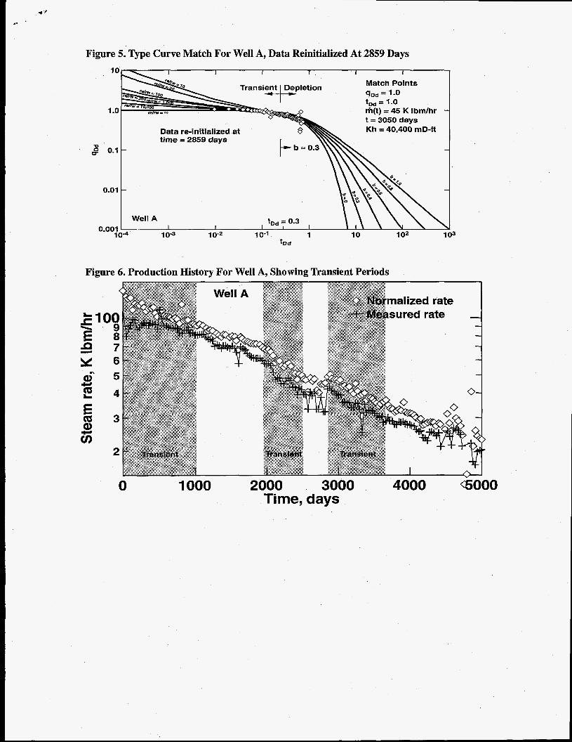
Figure 5. Type Curve Match For Well A, Data Reinitialized At 2859 Days 10

1 .o t = 3050 days Kh = 40,400 mD-ft

U 8 0.1

0.01

n nnq

Data re-initialized at time = 2859 days

-

-

Well A I I I.v-.

104 10” 10-2 lo-’ 1 10 102 103 *Dd

Figure 6. Production History For Well A, Showing Transient Periods

0 1000 2000 3000 Time, days

4000 6 0 0 0

(208) 526-0674 ti

Documents