202: dynamic macroeconomic...

202: Dynamic Macroeconomic TheoryFinancial Development & Growth:

Acemoglu & Zilibotti

Mausumi Das

Lecture Notes, DSE

Oct 1;8-9, 2015

Das (Lecture Notes, DSE) Dynamic Macro Oct 1;8-9, 2015 1 / 38

Financial Development & Growth: Diversification ofProduction Risks

We shall now examine another role of financial institution whichallows for the diversification of production risks, when the risk isaggregate (macro) in nature.

The paper that takes up this issue is:(Daron Acemoglu and Fabrizio Zilibotti: "Was PrometheusUnbound by Chance: Risk, Diversification and Growth", Journal ofPolitical Economy, 1997 (Vol. 105, pages 709-751)

Why "Prometheus Unbound"?Why "By Chance"?


Acemoglu & Zilibotti: Basic Idea

Consider an economy which faces aggreagte productivity shocks. Tofix ideas, this of these as weather/monsoon shocks: (i) poor monsoon(drought); (ii) normal monsoon; (iii) excess monsoon (flood)

Suppose that one can develop different varieties of seeds that givesthe same yield under different weather conditions:

Seed A works only when monsoon is poor;Seed B works only when monsoon is normal;Seed C works only when monsoon is excess.

But suppose developing each of these varieties of seeds requires aninitial fixed cost - in terms of R&D expenditure.

Then in a relatively poor country agents undertaking such R&Dactivities on their own may not be abale to cover the fixed costs of allthree types —hence they will be more vulnerable to such productivityshocks and output in these economies will fluctuate more.


Acemoglu & Zilibotti: Basic Idea (Contd.)

How do financial institutions help?

Financial institution helps by pooling all the resources of the agentstogether - therby increasing the probability of covering the fixed costsof each of these varieties.

In the process, it allows the economy to diversify the production risks.

If by pooling the reasouces, the financial institution is actually able tocover the fixed cost of all the three varietys, then the production riskwill be completely eliminated - no matter what the weather conditionis, the economy will always produce that same amount of output.


Acemoglu & Zilibotti: General Set Up

A closed economy producing a single final commodity which is usedfor consumption and savings.

Two period OLG structure: working when young; retired when old.

Let ’Ωt’denote the set of all young agents in period t. Population ineach generation is constant and consists of a continuum of agentsdistributed over an interval [0, a] where a > 1. Thus Ωt = [0, a].

Agents belonging to the same generation are identical in everyrespect.


Acemoglu & Zilibotti: Production Technology

A single final good, produced with the technology:

Yt = AK αt L

1−αt ; 0 < α < 1.

Competitive Market Structure (factors are paid their respectivemarginal products):

MPL = A(1− α)K αt L−αt

MPK = AαK α−1t L1−α

t

Let the total labour force be normalized to unity (i.e., Lt = 1).

Then the wage rate and the rental rate are respectively given by:

Wt = (1− α)AK αt L−αt

ρt = αAK α−1t L1−α

t

Capital depreciates fully upon production.


Acemoglu & Zilibotti: Technology for producing Capital

Capital is an intermediate good - which is producible and requires aninvestment of one time period and some resource investment in termsof the final commodity.

In particular there exists a continuum of projects - distributed over aunit mass - such that each project - under certain state - wouldtransform saving at time t to capital to be used in time (t + 1).

But the intermediate good production sector is characterized byuncertainty.

Uncertainty in the intermediate good sector is capture by thefollowing assumption:

there exists a continuum of mutually exclusive and equally likelystates - distributed over the unit interval [0, 1] . To fix ideas, you canthink these states as uniformly distributed over the interval [0, 1] .The intermediate sector j ∈ [0, 1] generates a positive return (in theform of some units of ‘capital’being produced) only under state j andzero return otherwise.


Acemoglu & Zilibotti: Technology for producing Capital(Contd.)

There is also a minimum size requirement in each intermediate goodsector, denoted by Mj .

An investment of Fj units of finals goods in sector j produces RFjunits of capital in the next period if and only if (i) state j is realized;and (ii) Fj = Mj .

The minimum size requirement varies across projects. In particular,for any j , the corresponding minimum size is given by:

Mj = Max0,

D1− γ

(j − γ)

,

where D is a positive constant and γ is another positive constantwhich is less then unity. The implication of this assumption is thefollowing. For all projects j 5 γ there is no mimmum sizerequirement; but for projects j > γ, the size requirement is positiveand increases linearly with the project index.


Minimum Size Requirement: In Diagram



There also exists a safe project that transforms saving at time t tocapital to be used in time (t + 1) under all realized states of thenature.

In other words, this technology is not characterized by uncertainty.

Under this safe project, an investment of φ units of finals goods insector j produces rφ units of capital in the next period.

We shall assume thatR > r .

Thus risky investments have a higher expected return than the safeasset.



Notice that the probability of success in different projects areimperfectly correlated/uncorrelated; so that there is safety in variety.

Consider a portfolio that consists of an equal amount of investment Fin all the risky projects belonging to some set J ⊂ [0, 1] .Let the probability measure of this set is p(J).

Then this portfolio pays the return RF with probability p(J) andnothing with probability 1− p(J).


Acemoglu & Zilibotti: Household Preferences

All agents - within a generation as well as across generations - haveidentical preferences.Preferences on an agent are represented by the following expectedutility function:

EtU(ct , ct+1) = log ct + β

1∫0

f (j) log c jt+1dj ; 0 < β < 1.

Notice that here j represents a state (not a project) and f (j) is theassociated probability density function.Since all the states are equally likely, f (j) = a constant for all j .Indeed if the distribution is uniform (defined over the unit interval)then f (j) = 1 for all j ∈ [0, 1], in which case we can write the aboveutility function as:

EtU(ct , ct+1) = log ct + β

1∫0

log c jt+1dj ; 0 < β < 1.


Life Cycle on an Young Agent:

Consider an young agent belonging to genertion t , identified byh ∈ Ωt = [0, a].

In the first period of his life (when young):

The agent is endowed with1aunits of labour and zero capital (no

intergenerational altruism; no bequest)The agent suppies his labour in the market in this period to earn a

wage income: wt = Wt1a

He consumes part of this wage income in the first period (ct ) and savesthat rest (st )The savings in turn is invested in various forms of projects (risky/safe)which would potentially generate some capital in the next periodThus in the first period, the agent also has to optimally decide on theportfolio over which his savings is to be distributed.


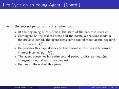
Life Cycle on an Young Agent: (Contd.)

In the second period of his life (when old):

At the beginning of this period, the state of the nature is revealed.Contingent on the realized state and the portfolio decisions made inthe previous period, the agent owns some capital stock at the beginingof this period: k jht+1He provides this capital stock to the market in this period to earn aninterest income: ρt+1k

jht+1

The agent consumes his entire second period capital earnings (nointergenrational altruism, no bequest).He dies at the end of this period.


Timing of Events:


Equity/Stock Market and Portfolio Decisions:

Investment in the ‘risky’(but more productive) intermediate goodprojects are mediated through the stock market.

We assume that the risky projects are run by young agents whocompete to get funds by issuing financial securities (Arrow securities)and selling them to other agents through the stock market.

Each agent can run at most one project, although more than oneagent can compete to run the same project.

An agent may even decide not to run any project at all.

In any case, the number/measure of project j ∈ [0, 1] being less thanthe number/measure of young agents h ∈ [0, a] , a > 1, in everyperiod there will always be some agents who will not be able tooperate any of the projects.


Equity/Stock Market and Portfolio Decisions: (Contd.)

The security market operates in two stages.

In stage I:

A young agent h ∈ Ωt declares pair: a project (j) which he wishes tooperate and the unit price of the corresponding security in terms of thefinal commodity at time t (Pj ,h,t ).We denote this announcement by agent h by the vectorZh , t ≡

(j ,Pj ,h,t

)∈ [0, 1]× R+

In announcing his own pair, agent takes similar announcements by allother agents as given.Let Zt summarize all such announcements by the agents such thatZt : Ωt −→ [0, 1]× R+And let Jt (Zt ) ⊆ [0, 1] be the set of all the projects for which there isat least a taker, i.e.,Jt (Zt ) =

j ∈ [0, 1] such that ∃h ∈ Ωt with Zh , t ≡

(j ,Pj ,h,t

)Once Jt (Zt ) is known, for each project j ∈ Jt (Zt ), the right to run theproject is awarded to the agent who has declared the minimum securityprice for that project.



Let Pt (Zt ) be the set of of such minimum prices for each projectj ∈ Jt (Zt ).Running such a project gives the operating agent an additionalincome in the form of a brokerage fee.

For each unit of investment made in any project j ∈ Jt (Zt ), theoperating agent channelises only a proportion

1Pj ,t

in the actual

project operation the and keeps the remaining proportionPj ,t − 1Pj ,t

as

his commission (brokerage fee).

Notice that the higher is Pj ,t , the higher is the eventual brokerage feeof the agent; but if the agent announces too high a Pj ,t , then he mightbe out-bidded and may not be awarded the project in the first place!In equilibrium, all the Pj ,t s will be such that nobody will have anincentive to deviate (in the Nash sense). We shall consider thecharateristics of such an equilibrium in a while.



In stage II:

Once all projects in the running and their minimum security prices (i.e,Jt (Zt ) and Pt (Zt )) have been specified, all agents take these as given.Then they optimally decide how much to invest in each of these riskyprojects vis-a-vis the safe project (which they can operate themselves).In the next period, once the state of the nature is revealed, two ofthese projects (one of the risky projects and the safe project) yieldreturns in the form of capital.These capital stock is then distributed to the investors in proportion totheir investments.The stock market closes thereafter.


Agents’Optimization Problem:

In light of the above characterization of the stock market, we canwrite an young agent’s optimization problem as:

Max. log ch,t + β

1∫0

log c jh,t+1dj

subject to

(i) ch,t + sh,t = wt + vjh,t ;

(ii) sh,t = φh,t + Ih,t , where It =∫

j∈Jt (Zt )

Pj ,tFjh,tdj ;

(iii) c jh,t+1 = ρjt+1

(rφh,t + RF

jh,t

)where

v jh,t ≡Pj ,t − 1Pj ,t

∫h∈Ωt

F jh,tdh ≡Pj ,t − 1Pj ,t

F jt if the agent operates project

j ∈ Jt (Zt ); is zero otherwise.Das (Lecture Notes, DSE) Dynamic Macro Oct 1;8-9, 2015 20 / 38

Households’Optimization Problem: (Contd.)

Notice that F jt = 0 if j /∈ Jt (Zt ).Moreover,

ρjt+1 = αA(K jt+1

)α−1= αA

∫h∈Ωt

(rφh,t + RF

jh,t

)dh

α−1

W jt+1 = (1− α)A

∫h∈Ωt

(rφh,t + RF

jh,t

)dh

α

Notice that in carrying out the optimization execise, the agents takesρjt+1as given. They also take Zt , Jt (Zt ) and Pt (Zt ) as given.

But Zt was offered by the agents themselves at stage I.

So how is Zt determined in the first place?


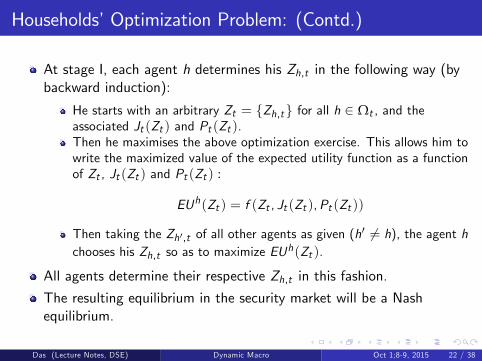
Households’Optimization Problem: (Contd.)

At stage I, each agent h determines his Zh,t in the following way (bybackward induction):

He starts with an arbitrary Zt = Zh,t for all h ∈ Ωt , and theassociated Jt (Zt ) and Pt (Zt ).Then he maximises the above optimization exercise. This allows him towrite the maximized value of the expected utility function as a functionof Zt , Jt (Zt ) and Pt (Zt ) :

EUh(Zt ) = f (Zt , Jt (Zt ),Pt (Zt ))

Then taking the Zh′,t of all other agents as given (h′ 6= h), the agent h

chooses his Zh,t so as to maximize EUh(Zt ).

All agents determine their respective Zh,t in this fashion.

The resulting equilibrium in the security market will be a Nashequilibrium.


Equilibrium in the Security Market: Characterization

Equilibrium in the security market is defined by a set Z ∗t and thecorresponding J∗t (Z

∗t ) and P

∗t (Z

∗t ) such that:

1 Each agent h chooses s∗h,t (P∗t , J

∗t ) , φ∗h,t (P

∗t , J

∗t ) , F

j∗h,t (P

∗t , J

∗t )

optimally;2 Z ∗t maximises EU

h(Zt ) for each h;3 The corresponding wage and rental rates are given by:

ρjt+1 = αA

∫h∈Ωt

(rφ∗h,t + RF

j∗h,t

)dh

α−1

;

W jt+1 = (1− α)A

∫h∈Ωt

(rφ∗h,t + RF

j∗h,t

)dh

α

.

Notice that the point (2) above implies that no agent will have anyincentive to change his announcement from Z ∗t to anything else.


Equilibrium in the Security Market: Characterization

There are several important features of this equilibrium:

1 At any such equilibrium configuration, v jh,t = 0 for all h (why?)2 At the equilibrium, all risky projects will be offered, i.e.,J∗t (Z

∗t ) = [0, 1] (why?)

3 In equilibrium, all young agents will have the same income and willchoose the same levels of s∗h,t , φ∗h,t ,and F

j∗h,t .

4 Since v jh,t =Pj ,t − 1Pj ,t

F jt = 0 in equilibrium, it follows that P∗j ,t = 1 for

all j5 Since every risky project has the same unit price as well as the sameexpected return, agents would invest equal amounts across all therisky projects, i.e.,

F j∗t = F j′∗t = F ∗t for all j , j

′ ∈ J∗t (Z ∗t )


Equilibrium Savings and Portfolio Choices:

Having identified the equilibrium in the security market (which weassume is reached instantaneously in every period - without specifyingthe exact mechanism), let us now examine the optimal savings andinvestment decisions of the agents.In doing that first note that although in equilibrium, all risky projectswill be offered, that does necessarily mean that all risky projects willactually be operational or open.Recall that there is a minimum size requirement for each such projectand unless the total investment on the project exceeds this, a project- even though offered - will not eventually be open.If every agent in equilibrium invest F ∗t in each of the risky projects,then total funds available for each project is: F ∗t =

∫h∈Ωt

F ∗t dh = aF∗t .

A project j ∈ [0, 1] will be open if and only if

aF ∗t ≥ Mj


Condition for a Project being Open: A DiagrammaticRepresentation

This diagram shows that even though all projects are offered, onlyprojects [0, n∗t ] will actually be open and projects (n

∗t , 1] will not be

open.Das (Lecture Notes, DSE) Dynamic Macro Oct 1;8-9, 2015 26 / 38

Condition for a Project being Open: (Contd.)

But even the above diagram is not strictly correct.Notice that here we have drawn aF ∗t as a flat line - independent ofthe no. of projects that are open.But if only [0, n∗t ] projects are open, than agents would not waste theirfunds on the (n∗t , 1] projects. They will spread their total investmentin risky projects (It) equally among the projects which are open.That is,

I ∗t = s∗t − φ∗t = n∗t F∗t

⇒ F ∗t =s∗t − φ∗tn∗t

In other words, F ∗t will be a function of n∗t as well. (Indeed, even s

∗t

and φ∗t might be functions of n∗t )

At the same time n∗t (the measure of how many projects would beopen) itself is a function of F ∗t .Thus F ∗t and n

∗t will be simultaneously determined from the agent’s

optimization problem.Das (Lecture Notes, DSE) Dynamic Macro Oct 1;8-9, 2015 27 / 38

Agents’Optimization Problem - Revisited:

In view of this, we can modify the representative agent’s optimizationproblem in the following way:Suppose the agent expects projects [0, nt ] ⊆ [0, 1] would be open.Recall that the probability that the realized state j ∈ [0, nt ] is givenby nt . Then the optimization problem of the young agent is given by:

Max. log ct + β

nt∫0

log c jt+1dj +

1∫nt

log c jt+1dj

subject to

(i) ct + st = wt

(ii) st = φt +

nt∫0

Ftdj

(iii) c jt+1 =ρjt+1 (rφt + RFt ) for j ∈ [0, nt ]

ρjt+1 (rφt ) for j ∈ (nt , 1]


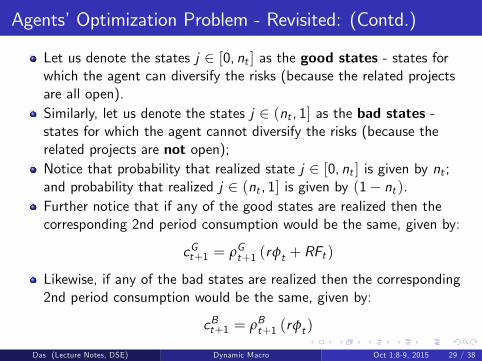
Agents’Optimization Problem - Revisited: (Contd.)

Let us denote the states j ∈ [0, nt ] as the good states - states forwhich the agent can diversify the risks (because the related projectsare all open).Similarly, let us denote the states j ∈ (nt , 1] as the bad states -states for which the agent cannot diversify the risks (because therelated projects are not open);Notice that probability that realized state j ∈ [0, nt ] is given by nt ;and probability that realized j ∈ (nt , 1] is given by (1− nt ).Further notice that if any of the good states are realized then thecorresponding 2nd period consumption would be the same, given by:

cGt+1 = ρGt+1 (rφt + RFt )

Likewise, if any of the bad states are realized then the corresponding2nd period consumption would be the same, given by:

cBt+1 = ρBt+1 (rφt )


Agents’Optimization Problem - Revisited: (Contd.)

In view of this, we can further modify the representative agent’soptimization problem in the following way:

Max. log ct + β[nt log cGt+1 + (1− nt ) log cBt+1

]subject to

(i) ct + st = wt(ii) st = φt + ntFt

(iii) cGt+1 = ρGt+1 (rφt + RFt )

(iv)cBt+1 = ρBt+1 (rφt )


Agents’Optimization Problem: Solution

Solving the above exercise, we get the following set of solutions:

s∗t =β

1+ βwt

φ∗t =(1− nt )R(R − nt r)

s∗t

F ∗t =(R − r)(R − nt r)

s∗t for all j ∈ [0, nt ] ; zero otherwise

(Verify)


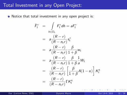
Total Investment in any Open Project:

Notice that total investment in any open project is:

F ∗t =∫

h∈Ωt

F ∗t dh = aF∗t

= a(R − r)(R − nt r)

s∗t

= a(R − r)(R − nt r)

β

1+ βwt

= a(R − r)(R − nt r)

β

1+ β

1aWt

=(R − r)(R − nt r)

[β

1+ βA(1− α)

]K αt

=(R − r)(R − nt r)

ΓK αt


Total Investment in any Open Project:

It is easy to verify thatdF ∗tdnt

> 0 andd2F ∗tdn2t

> 0.

Moreover, as nt → 0, F ∗t →(R − r)R

ΓK αt > 0

And as nt → 1, F ∗t → ΓK αt > 0

In other words, F ∗t is a convex function of nt , taking positive value atboth limits.

We already know that a project j ∈ [0, 1] will be open if and only if

F ∗t ≥ Mj

Having identified the exact F ∗t (nt ) function, we can now preciselyidentify which are the projects that would be open at time time t.


Number of Projects Open at time t : A DigrammaticRepresentation

Three possibilities:

Case 1: ΓK αt < D (Unique Intersection Point)



Case 2-a: ΓK αt > D (No Intersection Point)



Case 2-b: ΓK αt > D (Multiple Intersection Points)


Number of Projects Open at time t : Algebric Treatment

Optimal n∗t would be determined by the following equation:

F ∗t (nt ) =D(nt − γ)

1− γ

⇒ (R − r)(R − nt r)

ΓK αt =

D(nt − γ)

1− γ

⇒ r (nt )2 − (R + rγ) nt +

[(1− γ) (R − r)

(ΓD

)K αt + γR

]= 0

Solutions:

nt =(R + rγ)±

√(R + rγ)2 − 4r

[(1− γ) (R − r)

( ΓD

)K αt + γR

]2r

We shall assume that R = (2− γ)r - which rules out the possibilityof multiple intersection points when ΓK α

t > D. If also ensures thatwhen ΓK α

t < D, there is a unique intersection point within the range[0, 1] (given by the lesser value of the two roots).


Characterization of the T emporary Equilibrium at time t :

Under the above parametric assumption, given Kt , the static(temporary) equilibrium of the economy at time t is described asfollows:

Wt = A (1− α)K αt

ρt = AαK α−1t

s∗t =β

1+ βwt =

β

1+ β

1aWt =

1a

ΓK αt

φ∗t =(1− n∗t )R(R − n∗t r)

s∗t

F ∗t =(R − r)(R − n∗t r)

s∗t for all j ∈ [0, n∗t ] ; zero otherwise

n∗t =(R + rγ)−

√(R + rγ)2 − 4r

[(1− γ) (R − r)

( ΓD

)K αt + γR

]2r


202: dynamic macroeconomic...

Documents