2013 IEEE International Conference on Computer Vision

1550-5499/13 $31.00 © 2013 IEEE

DOI 10.1109/ICCV.2013.15

65

• The system is fully automatic and does not require

markers or any other specific settings for initialization.

• We perform feature-based tracking and mapping in

real time but leverage full inertial sensing in position

and orientation to estimate the metric scale of the re-

constructed 3D models and to make the process more

resilient to sudden motions.

• The system offers an interactive interface for casual

capture of scaled 3D models of real-world objects by

non-experts. The approach leverages the inertial sen-

sors to automatically select suitable keyframes when

the phone is held still and uses the intermediate mo-

tion to calculate scale. Visual and auditory feedback is

provided to enable intuitive and fool-proof operation.

• We propose an efficient and accurate multi-resolution

scheme for dense stereo matching which makes use of

the capabilities of the GPU and allows to reduce the

computational time for each processed image to about

2-3 seconds.

2. Related Work

Our work is related to several fields in computer vision:

visual inertial fusion, simultaneous localization and map-

ping (SLAM) and image-based modeling.

Visual inertial fusion is a well established technique [1].

Lobo and Dias align depth maps of a stereo head using

gravity as vertical reference in [6]. As their head is cal-

ibrated, they do not utilize linear acceleration to recover

scale. Weiss et al. [23] developed a method to estimate

the scaling factor between the inertial sensors (gyroscope

and accelerometer) and monocular SLAM approach and the

offsets between the IMU and the camera. Porzi et al. [12]

demonstrated a stripped-down version of a camera pose

tracking system on an Android phone where the inertial

sensors are utilized only to obtain a gravity reference and

frame-to-frame rotations.

Recently Li and Mourikis demonstrated impressive re-

sults on visual-inertial visual odometry, without recon-

structing the environment [5].

Klein and Murray [3] proposed a system for real-time

parallel tracking and mapping (PTAM) which was demon-

strated to work well also on smartphones [4]. Thereby, the

maintained 3D map is built from sparse point correspon-

dences only. Newcombe et al. [7] perform tracking, map-

ping and dense reconstruction on a high-end GPU in real

time on a commodity computer to create a dense model of

a desktop setup. Their approach makes use of general pur-

pose graphics processing but the required computational re-

sources and the associated power consumption make it un-

suitable for our domain.

As the proposed reconstruction pipeline is based on

stereo to infer geometric structure, it is related to a myr-

iad of works on binocular and multi-view stereo. We refer

to the benchmarks in [16], [17] and [19] for a representa-

tive list. However, most of those methods are not applicable

to our particular scenario as they don’t meet the underly-

ing efficiency requirements. In the following, we will focus

only on approaches which are conceptually closely related

to ours.

Building upon previous work on reconstruction with a

hand-held camera [10], Pollefeys et al. [11] presented a

complete pipeline for real-time video-based 3D acquisition.

The system was developed with focus on capturing large-

scale urban scenes by means of multiple video cameras

mounted on a vehicle. A method for real-time interactive

3D reconstruction was proposed by Stuehmer et al. [20].

Thereby, a 3D representation of the scene is obtained by

estimating depth maps from multiple views and convert-

ing them to triangle meshes based on the respective con-

nectivity. Another approach for live video-based 3D recon-

struction was proposed by Vogiatzis and Hernandez [22].

Here, the captured scene is represented by a point cloud

where each generated 3D point is obtained as a probabilis-

tic depth estimate by fusing measurements from different

views. Even though the aforementioned techniques cover

our context, they are designed for high-end computers and

are not functional on mobile devices due to some time-

consuming optimization operations.

Recently, the first works on live 3D reconstruction on

mobile devices appeared. Wendel et al. [24] rely on a dis-

tributed framework with a variant of [4] on a micro air vehi-

cle. All demanding computations are performed on a sepa-

rate server machine that provides visual feedback to a tablet

computer. Pan et al. [9] demonstrated an interactive system

for 3D reconstruction capable of operating entirely on a mo-

bile phone. However, the generated 3D models are not very

precise due to the sparse nature of the approach. Prisacariu

et al. [13] presented a shape-from-silhouette framework

running in real time on a mobile phone. Despite the im-

pressive performance, the method suffers from the known

weaknesses of silhouette-based techniques, e. g. the inabil-

ity to capture concavities. In contrast, the proposed system

does not exhibit these limitations since it relies on dense

stereo.

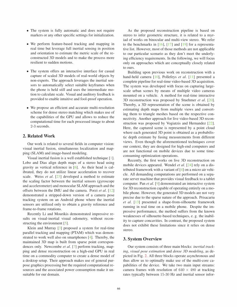
3. System Overview

Our system consists of three main blocks: inertial track-

ing, visual pose estimation and dense 3D modeling, as de-

picted in Fig. 2. All three blocks operate asynchronous and

thus allow us to optimally make use of the multi-core ca-

pabilities of the device. We take two main input streams:

camera frames with resolution of 640 × 480 at tracking

rates typically between 15-30 Hz and inertial sensor infor-

66

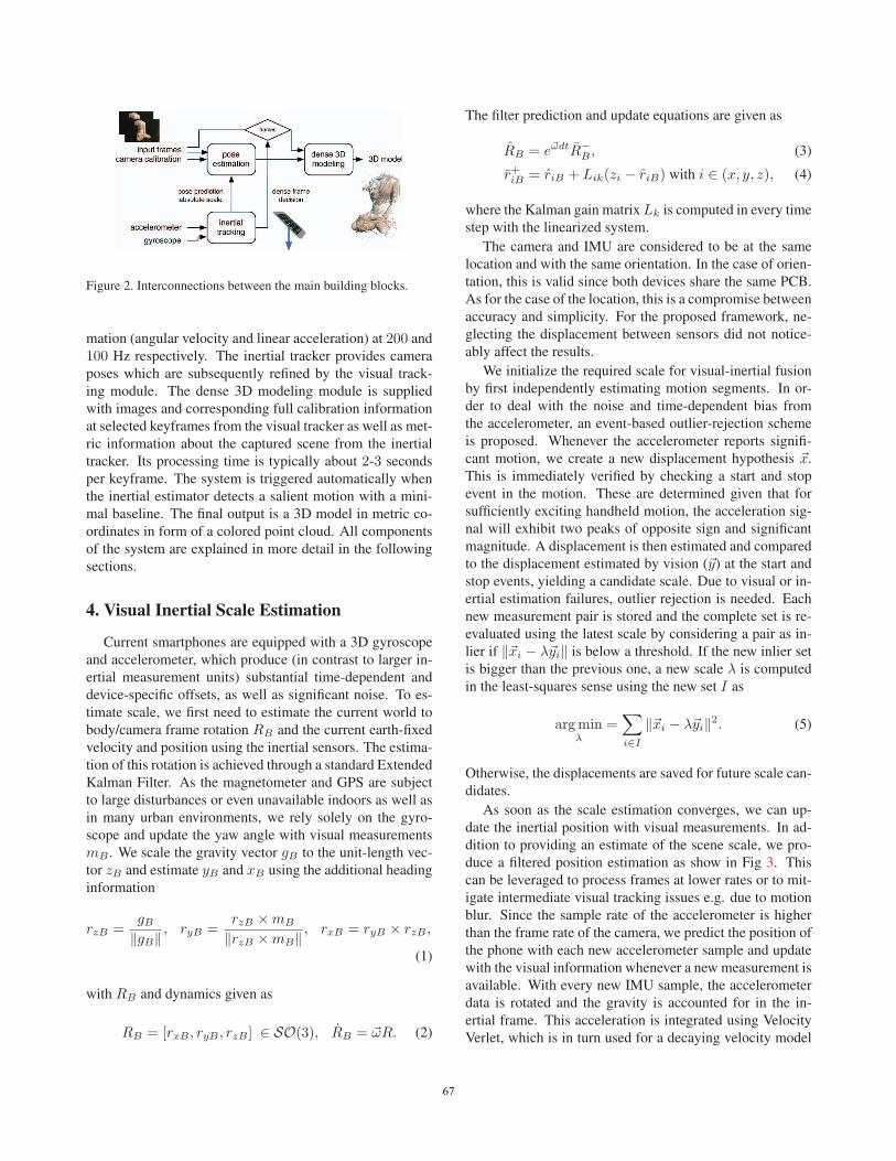
Figure 2. Interconnections between the main building blocks.

mation (angular velocity and linear acceleration) at 200 and

100 Hz respectively. The inertial tracker provides camera

poses which are subsequently refined by the visual track-

ing module. The dense 3D modeling module is supplied

with images and corresponding full calibration information

at selected keyframes from the visual tracker as well as met-

ric information about the captured scene from the inertial

tracker. Its processing time is typically about 2-3 seconds

per keyframe. The system is triggered automatically when

the inertial estimator detects a salient motion with a mini-

mal baseline. The final output is a 3D model in metric co-

ordinates in form of a colored point cloud. All components

of the system are explained in more detail in the following

sections.

4. Visual Inertial Scale Estimation

Current smartphones are equipped with a 3D gyroscope

and accelerometer, which produce (in contrast to larger in-

ertial measurement units) substantial time-dependent and

device-specific offsets, as well as significant noise. To es-

timate scale, we first need to estimate the current world to

body/camera frame rotation RB and the current earth-fixed

velocity and position using the inertial sensors. The estima-

tion of this rotation is achieved through a standard Extended

Kalman Filter. As the magnetometer and GPS are subject

to large disturbances or even unavailable indoors as well as

in many urban environments, we rely solely on the gyro-

scope and update the yaw angle with visual measurements

mB . We scale the gravity vector gB to the unit-length vec-

tor zB and estimate yB and xB using the additional heading

information

rzB =gB

‖gB‖, ryB =

rzB ×mB

‖rzB ×mB‖, rxB = ryB × rzB ,

(1)

with RB and dynamics given as

RB = [rxB , ryB , rzB ] ∈ SO(3), RB = �ωR. (2)

The filter prediction and update equations are given as

RB = e�ωdtR−

B , (3)

r+iB = riB + Lik(zi − riB) with i ∈ (x, y, z), (4)

where the Kalman gain matrix Lk is computed in every time

step with the linearized system.

The camera and IMU are considered to be at the same

location and with the same orientation. In the case of orien-

tation, this is valid since both devices share the same PCB.

As for the case of the location, this is a compromise between

accuracy and simplicity. For the proposed framework, ne-

glecting the displacement between sensors did not notice-

ably affect the results.

We initialize the required scale for visual-inertial fusion

by first independently estimating motion segments. In or-

der to deal with the noise and time-dependent bias from

the accelerometer, an event-based outlier-rejection scheme

is proposed. Whenever the accelerometer reports signifi-

cant motion, we create a new displacement hypothesis �x.

This is immediately verified by checking a start and stop

event in the motion. These are determined given that for

sufficiently exciting handheld motion, the acceleration sig-

nal will exhibit two peaks of opposite sign and significant

magnitude. A displacement is then estimated and compared

to the displacement estimated by vision (�y) at the start and

stop events, yielding a candidate scale. Due to visual or in-

ertial estimation failures, outlier rejection is needed. Each

new measurement pair is stored and the complete set is re-

evaluated using the latest scale by considering a pair as in-

lier if ‖�xi − λ�yi‖ is below a threshold. If the new inlier set

is bigger than the previous one, a new scale λ is computed

in the least-squares sense using the new set I as

argminλ

=∑

i∈I

‖�xi − λ�yi‖2. (5)

Otherwise, the displacements are saved for future scale can-

didates.

As soon as the scale estimation converges, we can up-

date the inertial position with visual measurements. In ad-

dition to providing an estimate of the scene scale, we pro-

duce a filtered position estimation as show in Fig 3. This

can be leveraged to process frames at lower rates or to mit-

igate intermediate visual tracking issues e.g. due to motion

blur. Since the sample rate of the accelerometer is higher

than the frame rate of the camera, we predict the position of

the phone with each new accelerometer sample and update

with the visual information whenever a new measurement is

available. With every new IMU sample, the accelerometer

data is rotated and the gravity is accounted for in the in-

ertial frame. This acceleration is integrated using Velocity

Verlet, which is in turn used for a decaying velocity model

67

84 86 88 90 92 94 96 98 100−0.3

−0.28

−0.26

−0.24

−0.22

−0.2

−0.18

−0.16

−0.14

−0.12

time [seconds]

Effects of filter (Z−axis)

Vicon

scaled Vision

scaled IMU+Vision

20 25 30 35 40 45 5010

−2

10−1

Convergence of scale estimation

time [seconds]

Estimated scale

Real scale

9 10 11 12 13 14 15 16−1.4

−1.2

−1

−0.8

−0.6

−0.4

−0.2

0

0.2

0.4

0.6Position (z−axis)

time [seconds]

m

Decay model

Direct integration

Ground truth

Figure 3. Left: simple inertial prediction and decaying velocity

vs ground truth. Right: visual-inertial estimate allows to partially

reject tracking losses. Bottom: Convergence of scale estimation.

of handheld motion

�v k+1

I = �v kI + τΔtRB

(�a kB − gB

). (6)

Here τ accounts for timing and sensor inaccuracies (inher-

ent of the operating system available on mobile phones) by

providing a decaying velocity model, preventing unwanted

drift at small accelerations (see Fig 3). To adapt to the vi-

sual data, it is first scaled to metric units using λ and then

fused with the inertial prediction using a simple linear com-

bination based on the variances of both estimations

�xf = κ(σ−2v λ �xv + σ−2

i �xi

). (7)

Here the subscripts f , v and i denote fused, vision and in-

ertial position estimates, respectively, and κ is the normal-

izing factor.

The visual updates become available with a time offset,

so we need to re-propagate the predicted states from the

point, at which the vision measurement occurred, to the cur-

rent one [23]. This is done by storing the sates in a buffer

and, whenever a visual measurement arrives, looking back

for the closest time-stamp in that buffer, updating and prop-

agating forward to the current time.

Fig 4 shows the results of the combined vision and iner-

tial fusion in a freehand 3D motion while tracking a table-

top scenario. It is evident that scale and absolute position

are correctly estimated throughout the trajectory.

To evaluate the estimated scale accuracy, metric recon-

struction of a textured cylinder with a known diameter was

performed. In a qualitative evaluation with multiple tries,

the scale was estimated to have an error of up to 10-15%.

This is mostly due to the inaccuracy in the magnitude of the

measurements of the consumer-grade accelerometer on the

−0.3

−0.2

−0.1

0

00.1

0.2

−0.05

0

0.05

0.1

0.15

0.2

y[m]

Scaled 3D trayectory

x[m]

z[m

]

scaled pose

VICON

scaled map points

Table

Figure 4. Visual inertial pose estimate vs. ground truth.

device. It should be noted that the accuracy of those mea-

surements could be improved by calibrating the accelerom-

eter with respect to the camera beforehand, but such inves-

tigations are left for future work.

5. Visual Tracking and Mapping

5.1. Two View Initialization

The map is initialized from two keyframes. ORB fea-

tures [14] are extracted from both frames and matched. Out-

liers are filtered out by using the 5-point algorithm in com-

bination with RANSAC. After that, relative pose optimiza-

tion is performed and the point matches are triangulated.

The rest of the initialization follows the design of [3]: In

order to get a denser initial map, FAST corners are then ex-

tracted on four resolution levels and for every corner a 8x8

pixel patch at the respective level is stored as descriptor.

The matching is done by comparing the zero-mean sum of

squared differences (ZSSD) value between the pixel patches

of the respective FAST corners along the epipolar line. To

speed up the process, only the segment of the epipolar line

is searched that matches the estimated scene depth from the

already triangulated points. After the best match is found,

the points are triangulated and included to the map which

is subsequently refined with bundle adjustment. Since the

gravity vector is known from the inertial estimator, the map

is also rotated such that it matches the earth inertial frame.

5.2. Patch Tracking and Pose Refinement

The tracker is used to refine the pose estimate from the

inertial pose estimator and to correct drift. For every new

camera frame FAST corners are extracted and matched with

68

the projected map points onto the current view using the in-

ertial pose. The matching is done by warping the 8x8 pixel

patch of the map point onto the view of the current frame

and computing the ZSSD score. It is assumed that its nor-

mal is oriented towards the camera that observed it for the

first time. For computing the warp the appropriate pyra-

mid level in the current view is selected. The best matching

patch in a certain pixel radius is accepted. The matches are

then optimized with a robust Levenberg-Marquart absolute

pose estimator giving the new vision-based pose for the cur-

rent frame. If for some reason the tracking is lost the small

blurry image relocalization module from [3] is used.

5.3. Sparse Mapping

New keyframes are added to the map if the user has

moved the camera a certain amount or if the inertial position

estimator detects that the phone is held still after salient mo-

tion. In either case, the keyframe is provided to the mapping

thread that accepts the observations of the map points from

the tracker and searches for new ones. To this end, a list of

candidates is created from non maximum suppressed FAST

corners that have a Shi-Tomasi score [18] above a certain

threshold. To minimize the possibility that new points are

created at positions where such already exist, a mask is cre-

ated to indicate the already covered regions. No candidate

is added to the map if its projection is inside a certain pixel

radius. Since the typical scene consists of an object in the

middle of the scene, only map points that were observed

from an angle of 60 degrees or less relative to the current

frame are added to this mask. This allows to capture both

sides of the object but still reduces the amount of duplicates.

Similar to [3], the mapper performs bundle adjustment

optimization in the background. Its implementation is based

on the method using the Schur complement trick that is

described in [2]. After a keyframe is added, a local bun-

dle adjustment step with the closest 4 keyframes is per-

formed. With a reduced priority, the mapper optimizes the

keyframes that are prepared for the dense modeling module.

Frames, that have already been provided to the module, are

marked as fixed. With lowest priority, the mapping thread

starts global bundle adjustment optimization based on all

frames and map points. This process is interrupted if new

keyframes arrive.

6. Dense 3D Modeling

At the core of the 3D modeling module is a stereo-based

reconstruction pipeline. In particular, it is composed of

image mask estimation, depth map computation and depth

map filtering. In the following, each of these steps is dis-

cussed in more detail. Finally, the filtered depth map is back

projected to 3D, colored with respect to the reference image

and merged with the current point cloud.

6.1. Image Mask Estimation

The task of the maintained image mask is twofold. First,

it identifies pixels exhibiting sufficient material texture.

This allows to avoid unnecessary computations which have

no or negligible effect on the final 3D model and reduces

potential noise. Second, it overcomes the generation of re-

dundant points by excluding regions already covered by the

current point cloud.

A texture-based mask is computed by reverting to the

Shi-Tomasi measure used also at the visual tracking stage

(see Section 5). The mask is obtained by thresholding the

values at some λmin > 0. In our implementation, we set

λmin = 0.1 and use patch windows of size 3×3 pixels. Ad-

ditionally, another mask is estimated based on the coverage

of the current point cloud. To this end, a sliding window,

which contains a set of the recently included 3D points, is

maintained. All points are projected onto the current image

and a simple photometric criterion is evaluated. Note that

points, that belong to parts of the scene not visible in the

current view, are unlikely to have erroneous contribution to

the computed coverage mask. The final image mask is ob-

tained by fusing the estimated texture and coverage mask.

Subsequent depth map computations are restricted to pixels

within the mask.

6.2. Depth Map Computation

Multi-resolution scheme. We run binocular stereo by

taking an incoming image as a reference view and match-

ing it with an appropriate recent image in the provided se-

ries of keyframes. Instead of applying a classical technique

based on estimating the optimal similarity score along re-

spective epipolar lines, we adopt a multi-resolution scheme.

The proposed approach involves downsampling the input

images, estimating depths, and subsequently upgrading and

refining the results by restricting computations to a suitable

pixel-dependent range.

Similar to the visual tracking stage (see Section 5), we

rely on computations at multiple pyramid resolutions. At

each level i ∈ {0, . . . , L}, respective images are obtained

by halving the resolution of their versions at level i − 1 in

each dimension. Thereby, i = 0 contains the original im-

ages. Starting at the top of the pyramid, the multi-resolution

approach estimates a depth map Di : Ωi ⊂ Z2 → R ⊂ R

to each level i based on the image data at that level and

the depth map from the consecutive level Di+1. While ex-

haustive computations have to be performed for the highest

level L, subsequent computational efforts can be reduced

significantly by exploiting the previously obtained coarse

result. In particular, we apply an update scheme based on

the current downsampled pixel position and three appropri-

ate neighbors. For example, for pixel (x, y) ∈ Ωi with xmod 2 = 1 and ymod 2 = 1 (the remaining cases are han-

dled analogously) we consider the following already pro-

69

Figure 5. Single- vs. multi-resolution depth map estimation. From

left to right: The reference image of a stereo pair, correspond-

ing depth map estimated with a classical single-resolution winner-

takes-all strategy and result obtained with the proposed multi-

resolution scheme.

vided depth values

D0i+1 = Di+1(x

′, y′)

D1i+1 = Di+1(x

′ + 1, y′)

D2i+1 = Di+1(x

′ + 1, y′ + 1)

D3i+1 = Di+1(x

′, y′ + 1),

(8)

where (x′, y′) := (�x/2�, �y/2�) ∈ Ωi+1. We estimate the

depth Di(x, y) by searching an appropriate range given by

the minimum and maximum value in {Dli+1 |l = 0, . . . , 3}.

Thereby, depth values, that are not available due to bound-

ary constraints or the maintained image mask, are omitted.

In order to take into account uncertainties due to the coarse

sampling at higher pyramid levels, we additionally include

a small tolerance in the estimated ranges. As the uncer-

tainty is expected to increase with increasing depth due to

the larger jumps of the values from pixel to pixel, we use

a tolerance parameter which is inversely proportional to the

local depth D0i+1.

In our implementation, we used images of size 640×480pixels and 3 resolution levels (i.e. L = 2). It should be

noted that all estimated depth maps rely on a predefined

range R ⊂ R which can be determined by analyzing the

distribution of the sparse map constructed in the camera

tracking module (see Section 5).

The multi-resolution scheme comes along with some

important advantages. First, it entails significant effi-

ciency benefits compared to traditional methods as epipo-

lar line traversals at higher image resolutions are restricted

to short segments. Second, when applying a winner-takes-

all strategy, potential mismatches can be avoided due to

the more robust depth estimates at low image resolution.

Third, regions in the image, which belong to distant scene

parts outside of the range of interest, can be discarded

at the lowest resolution level and subsequent refinement

operations can be avoided for them. To illustrate these

aspects, we present a comparison between the classical

single-resolution winner-takes-all strategy and the devel-

oped multi-resolution technique on an example image pair

(see Fig. 5). While both results look genuinely similar,

a closer look reveals that the proposed multi-resolution

scheme confers a higher degree of robustness by producing

less outliers. Note that for the above example a conserva-

tive depth range was used so as to capture the entire field

of view. However, the real benefit from it becomes evident

when comparing the respective runtimes. In practice, the

multi-resolution approach is about 5 times faster than the

single-resolution counterpart.

GPU acceleration. Despite the utilization of a multi-

resolution scheme, the developed method for dense stereo is

not efficient enough to meet the requirements of the applica-

tion at hand. For this reason, we made use of the paralleliza-

tion potential of the algorithm with a GPU implementation

(based on GLSL ES), which reduces the overall runtime of

the 3D modeling module to about 2-3 seconds per processed

image. More concretely, we estimate depth maps at differ-

ent pyramid levels in separate rendering passes. Thereby,

some care should be taken due to the precision limitations

of current mobile GPUs. We address this difficulty by using

the sum of absolute differences (SAD) as a similarity mea-

sure in the matching process (over 5×5 image patches) and

transferring triangulation operations to get the final depth

estimates to the CPU.

Image pair selection. A crucial step in binocular stereo is

the choice of an appropriate image pair. An ideal candidate

pair should share a large common field of view, a small but

not too small baseline and similar orientations. As we have

an ordered image sequence, a straightforward methodology

would be to match each incoming image with its predeces-

sor. Yet, this strategy is suboptimal in some cases, for ex-

ample when the user decides to move back and recapture

certain parts of the scene. Instead, we propose to maintain a

sliding window containing the last Nv provided keyframes

(Nv = 5 in our implementation) and pick the one maximiz-

ing a suitable criterion for matching with the current view.

For two cameras j and k this criterion is defined as

C(j, k) = cos θjkpose · cos θjkview · cos θjkup, (9)

where θjkpose denotes the angle between the viewing rays of

both cameras at the midpoint of the line segment connect-

ing the mean depth range points along the camera principal

rays, θjkview is the angle between the principal rays and θjkupis the angle between the up vectors of both cameras. Addi-

tionally, we impose the following constraints

5◦ ≤ θjkpose ≤ 45◦, 0◦ ≤ θjkview ≤ 45◦, 0◦ ≤ θjkup ≤ 30◦

An input image is discarded and not processed if none of

the images in the current sliding window satisfy those con-

straints with respect to it.

70

71

72