2011yangjphd
TRANSCRIPT

Glasgow Theses Service http://theses.gla.ac.uk/
Yang, Jin (2011) Fault analysis and protection for wind power generation systems. PhD thesis. http://theses.gla.ac.uk/2420/ Copyright and moral rights for this thesis are retained by the author A copy can be downloaded for personal non-commercial research or study, without prior permission or charge This thesis cannot be reproduced or quoted extensively from without first obtaining permission in writing from the Author The content must not be changed in any way or sold commercially in any format or medium without the formal permission of the Author When referring to this work, full bibliographic details including the author, title, awarding institution and date of the thesis must be given
Fault Analysis and Protection for Wind Power Generation Systems
Jin Yang
Submitted in fulfilment of the requirements for the degree of Doctor of Philosophy (Ph.D.)
Electronics and Electrical Engineering School of Engineering
College of Science and Engineering University of Glasgow
March 2011 Copyright © Jin Yang

To my family …

i
Abstract
Wind power is growing rapidly around the world as a means of dealing with the
world energy shortage and associated environmental problems. Ambitious plans
concerning renewable energy applications around European countries require a
reliable yet economic system to generate, collect and transmit electrical power from
renewable resources. In populous Europe, collective offshore large-scale wind farms
are efficient and have the potential to reach this sustainable goal. This means that an
even more reliable collection and transmission system is sought. However, this
relatively new area of offshore wind power generation lacks systematic fault
transient analysis and operational experience to enhance further development. At the
same time, appropriate fault protection schemes are required.
This thesis focuses on the analysis of fault conditions and investigates effective fault
ride-through and protection schemes in the electrical systems of wind farms, for both
small-scale land and large-scale offshore systems. Two variable-speed generation
systems are considered: doubly-fed induction generators (DFIGs) and permanent
magnet synchronous generators (PMSGs) because of their popularity nowadays for
wind turbines scaling to several-MW systems. The main content of the thesis is as
follows. The protection issues of DFIGs are discussed, with a novel protection
scheme proposed. Then the analysis of protection scheme options for the fully rated
converter, direct-driven PMSGs are examined and performed with simulation
comparisons. Further, the protection schemes for wind farm collection and
transmission systems are studied in terms of voltage level, collection level − wind
farm collection grids and high-voltage transmission systems for multi-terminal DC
connected transmission systems, the so-called “Supergrid”. Throughout the thesis,
theoretical analyses of fault transient performances are detailed with
PSCAD/EMTDC simulation results for verification. Finally, the economic aspect for
possible redundant design of wind farm electrical systems is investigated based on
operational and economic statistics from an example wind farm project.

ii
Acknowledgements
Firstly, I would like to express the deepest gratitude to my supervisor Professor John
O’Reilly for taking me under supervision after changes to my Ph.D. study. He is so
kind in his support and advice. I would also like to thank my second supervisor Dr.
John E. Fletcher formerly at the University of Strathclyde (now with the University
of New South Wales, Sydney, Australia) for much technical guidance. Thanks also to
Dr. David G. Dorrell (now with the University of Technology, Sydney, Australia) for
giving me this opportunity to pursue a Ph.D. degree at the University of Glasgow.
The financial support for this research project given by the Scottish Funding Council
in name of Glasgow Research Partnership in Engineering (GRPE) is gratefully
acknowledged. Thanks are also due to the Department of Electronics and Electrical
Engineering for support in academic visits, in particular Professor John M. Arnold
and Dr. Scott Roy.
Further, many thanks go to my friends and colleagues in the Power System and
Power Electronics Group in Electronics and Electrical Engineering, especially Ms.
Laura Nicholson, Mr. Sze Song Ngu, Mr. Majid Mumtaz, and Mr. Bazad
Kazemtabrizi, for making the working environment enjoyable. I would like to thank
the project group at the University of Strathclyde, consisting of Dr. Huibin Zhang,
Mr. Shixiong Fan, and Mr. Yuanye Xia. They are all gratefully acknowledged for
providing valuable input during the project.
Finally, I would like to thank my family for their love and support throughout.
iii
Table of Contents
Abstract ......................................................................................................................... i
Acknowledgements ............................................................................................................. ii
Table of Contents ............................................................................................................... iii
List of Figures ................................................................................................................... vii
List of Tables .................................................................................................................... xiii
Abbreviations and Nomenclature .................................................................................... xiv
Chapter 1 Introduction ....................................................................................................... 1 1.1 Wind Energy Industry...................................................................................... 1 1.2 Objectives and Motivation of the Thesis ......................................................... 3 1.3 Wind Power Generation Systems .................................................................... 5
1.3.1 Doubly-Fed Induction Generators....................................................... 5 1.3.2 Permanent Magnet Synchronous Generators .................................... 12
1.4 Wind Power Collection and Transmission Technologies ............................... 14 1.4.1 Collection Grid.................................................................................. 14 1.4.2 High-Voltage Direct-Current Transmission....................................... 15
1.5 Protection Development of DC Systems ....................................................... 20 1.6 Outline of Thesis ........................................................................................... 23 1.7 List of Publications........................................................................................ 25 1.8 References ..................................................................................................... 27
Chapter 2 Doubly-Fed Induction Generator Fault Protection Schemes ...................... 34 2.1 Introduction ................................................................................................... 34 2.2 Converter Protection Schemes for DFIG....................................................... 35
2.2.1 Crowbar Protection ........................................................................... 35 2.2.2 DC-Chopper ...................................................................................... 36 2.2.3 Series Dynamic Resistor ................................................................... 36
2.3 DFIG Rotor Currents during Fault Conditions.............................................. 38 2.3.1 Symmetrical Fault Conditions........................................................... 39 2.3.2 Asymmetrical Fault Conditions......................................................... 40
2.4 Protection Scheme Based on Series Dynamic Resistor ................................. 45 2.4.1 Switching Strategy ............................................................................ 46 2.4.2 Series Dynamic Resistance Calculations........................................... 47
2.5 Simulation Results......................................................................................... 48

iv
2.5.1 Symmetrical Fault Condition ............................................................ 49 2.5.2 Asymmetrical Fault Conditions......................................................... 52 2.5.3 Performance Comparison Between Crowbar and SDR..................... 55
2.6 Application Discussions ................................................................................ 57 2.6.1 Switch Time of the Bypass Switch.................................................... 57 2.6.2 Switch Normal Operation Losses...................................................... 57
2.7 Conclusion..................................................................................................... 57 2.8 References ..................................................................................................... 59
Chapter 3 Permanent Magnet Synchronous Generator Fault Protection Schemes .... 61 3.1 Introduction ................................................................................................... 61 3.2 Direct-Driven PMSG Wind Power Generation Systems ............................... 62
3.2.1 PMSG Power Conversion Topologies............................................... 62 3.2.2 Control Strategy ................................................................................ 64
3.3 PMSG System Protection .............................................................................. 64 3.3.1 Large-Scale System Protection.......................................................... 65 3.3.2 Small-Scale System Protection ......................................................... 67
3.4 Simulation Results......................................................................................... 70 3.4.1 Large-Scale System Fault Condition................................................. 71 3.4.2 Small-Scale System Fault Condition................................................. 74
3.5 Conclusion..................................................................................................... 78 3.6 References ..................................................................................................... 79
Chapter 4 Internal Fault Analysis and Protection of Multi-terminal DC Wind Farm Collection Grids ................................................................................ 81
4.1 Introduction ................................................................................................... 81 4.2 Multi-terminal DC Wind Farm ...................................................................... 83
4.2.1 Multi-terminal DC Wind Farm Topology.......................................... 83 4.2.2 DC Distribution System Fault Protection.......................................... 84
4.3 DC Fault Types and Characteristics............................................................... 85 4.3.1 VSI DC Short-Circuit Fault Overcurrent .......................................... 86 4.3.2 VSI DC Cable Ground Fault ............................................................. 91 4.3.3 DC Cable Open-Circuit Fault............................................................ 95 4.3.4 Multi-level Voltage-Source Converters ............................................. 95 4.3.5 Fault Characteristic Summary ........................................................... 96
4.4 DC Fault Protection Methods ........................................................................ 97 4.4.1 DC Switchgear .................................................................................. 97 4.4.2 Measurement and Relaying Configuration........................................ 98

v
4.4.3 Small-Scale System Protection Option ........................................... 105 4.5 DC Wind Farm Protection Simulation Results ............................................ 106
4.5.1 Short-Circuit Fault Condition.......................................................... 107 4.5.2 Cable Ground Fault Condition ........................................................ 109
4.6 Ground Fault Location and Resistance Evaluation ......................................111 4.7 Conclusion................................................................................................... 118 4.8 References ................................................................................................... 120
Chapter 5 Protection Coordination of Meshed VSC-HVDC Transmission Systems for Large-Scale Wind Farms .................................................................... 122
5.1 Introduction ................................................................................................. 122 5.2 Multi-terminal Meshed DC Wind Farm Network ....................................... 123
5.2.1 Meshed Multi-terminal DC Wind Farm Topology .......................... 123 5.2.2 Supergrid Section for Protection Test Study ................................... 124
5.3 DC Fault Analysis for Large-Scale Meshed Systems.................................. 127 5.3.1 Appropriate Cable Modelling for DC Fault Analysis...................... 127 5.3.2 DC Bus Fault ................................................................................... 130
5.4 Protection Scheme for Meshed DC Systems ............................................... 131 5.4.1 High-Power DC Switchgear Allocation .......................................... 131 5.4.2 DC CB Relay Coordination Relations............................................. 134 5.4.3 Protection Scheme........................................................................... 135 5.4.4 Protective Selection without Relay Communication....................... 138
5.5 DC Wind Farm Protection Simulation Results ............................................ 141 5.5.1 DC Radial Cable Short-Circuit/Ground Fault Condition ................ 141 5.5.2 DC Loop Cable Short-Circuit/Ground Fault Condition .................. 143 5.5.3 DC Bus Short-Circuit/Ground Fault Condition............................... 144 5.5.4 Cable Modelling Comparison ......................................................... 146
5.6 Conclusion................................................................................................... 147 5.7 References ................................................................................................... 149
Chapter 6 Reliability Enhancement of Offshore Wind Farms by Redundancy Analysis ...................................................................................................... 151
6.1 Introduction ................................................................................................. 151 6.2 Wind Farm Collection/Transmission Systems and Reliability .................... 152
6.2.1 Collection Grids .............................................................................. 152 6.2.2 Transmission Systems ..................................................................... 153 6.2.3 Wind Farm Collection and Transmission System Reliability
Assessment ..................................................................................... 154

vi
6.3 Wind Farm Collection and Transmission System Redundancy Definition.... 154 6.3.1 Topology Redundancy..................................................................... 154 6.3.2 Device Redundancy......................................................................... 155 6.3.3 Redundancy Definition.................................................................... 156
6.4 Wind Farm Redundancy Design.................................................................. 159 6.4.1 Offshore Wind Farm Layout Feature .............................................. 159 6.4.2 The Design Process Description...................................................... 160 6.4.3 Choice of Transformer Platform Number and Location.................. 160 6.4.4 Normal Collection Grid Topology Design ...................................... 162 6.4.5 Redundancy Design......................................................................... 162
6.5 Example Wind Farm Design Analysis......................................................... 164 6.5.1 Reliability Assessment .................................................................... 165 6.5.2 Economic Assessment ..................................................................... 165 6.5.3 Summary and Comparison .............................................................. 166
6.6 Conclusion................................................................................................... 169 6.7 References ................................................................................................... 171
Chapter 7 Conclusions and Future Work...................................................................... 173 7.1 Conclusions ................................................................................................. 173 7.2 Future Work ................................................................................................. 175
vii
List of Figures
Figure 1.1: Doubly-fed induction generator system and its power flows........................................... 6 Figure 1.2: DFIG mechanical power, generator stator power and rotor power in per unit
(Pm, Ps, and Pr) in respect to rotor slip s. ......................................................................... 9 Figure 1.3: Large-scale PMSG power conversion system topology. ................................................ 12 Figure 1.4: Small-scale PMSG power conversion system topology................................................. 13 Figure 2.1: DFIG rotor equivalent circuit with all protection schemes shown................................. 38 Figure 2.2: Comparison of simulation and theoretical rotor currents during fault
conditions (for 0.5 s): (a) three-phase 1.0 p.u. voltage dip; (b) three-phase 0.6 p.u. voltage dip; (c) single-phase (phase a) voltage dip of 1.0 p.u.; (d) phase-to-phase (phase b to c) short circuit..................................................................... 44
Figure 2.3: Three-phase rotor currents during different fault conditions (for 0.5 s): (a) three-phase 1.0 p.u. voltage dip; (b) three-phase 0.6 p.u. voltage dip; (c) single-phase (phase a) 1.0 p.u. voltage dip; (d) phase-to-phase (phase b to c) short circuit. ................................................................................................................... 45
Figure 2.4: Combined converter protection switching strategy (for subscripts: th – threshold values; CB – Crowbar; SDR – Series Dynamic Resistor). ............................. 47
Figure 2.5: Three-phase 0.95 p.u. voltage dip for 0.2 s without protection: (a) three-phase stator voltages vs a,b,c [in per unit (p.u.)]; (b) three-phase stator currents is a,b,c (p.u.); (c) three-phase rotor currents ir a,b,c (p.u.); (d) phase-a rotor voltage vra (p.u.) and phase-a RSC voltage vrsc,a (p.u.); (e) DC-link voltage vDC (p.u.); (f) stator side active power Ps (p.u.) and reactive power Qs (p.u.); (g) rotor speed ωr (p.u.); (h) electrical torque Te (p.u.) and mechanical torque Tm (p.u.). .......................................................................................... 50
Figure 2.6: Three-phase 0.95 p.u. voltage dip for 0.2 s with converter protection: (a) three-phase stator voltages vs a,b,c [in per unit (p.u.)]; (b) three-phase stator currents is a,b,c (p.u.); (c) three-phase rotor currents ir a,b,c (p.u.); (d) SDR switching signal SSDR; (e) crowbar switching signal SCB; (f) DC-chopper switching signal SDCC; (g) phase-a rotor voltage vra (p.u.) and phase-a RSC voltage vRSC,a (p.u.); (h) DC-link voltage vDC (p.u.); (i) stator side active power Ps (p.u.) and reactive power Qs (p.u.); (j) rotor speed ωr (p.u.); (k) electrical torque Te (p.u.) and mechanical torque Tm (p.u.)............................................ 51
Figure 2.7: The rotor voltage vra [in per unit (p.u.)] and rotor-side converter voltage vRSC,a (p.u.) comparison (zoomed from 1 s to 1.1 s)....................................................... 52
Figure 2.8: Phase-a 1.0 p.u. voltage dip for 0.2 s with converter protection: (a) three-phase stator voltages vs a,b,c [in per unit (p.u.)]; (b) three-phase stator currents is a,b,c (p.u.); (c) three-phase rotor currents ir a,b,c (p.u.); (d) SDR

viii
switching signal SSDR; (e) crowbar switching signal SCB; (f) DC-chopper switching signal SDCC; (g) phase-a rotor voltage vra (p.u.) and phase-a RSC voltage vRSC,a (p.u.); (h) DC-link voltage vDC (p.u.); (i) stator side active power Ps (p.u.) and reactive power Qs (p.u.); (j) rotor speed ωr (p.u.); (k) electrical torque Te (p.u.) and mechanical torque Tm (p.u.)............................................ 53
Figure 2.9: Phase b to c short circuit for 0.2 s with converter protection: (a) three-phase stator voltages vs a,b,c [in per unit (p.u.)]; (b) three-phase stator currents is a,b,c (p.u.); (c) three-phase rotor currents ir a,b,c (p.u.); (d) SDR switching signal SSDR; (e) crowbar switching signal SCB; (f) DC-chopper switching signal SDCC; (g) phase-a rotor voltage vra (p.u.) and phase-a RSC voltage vRSC,a (p.u.); (h) DC-link voltage vDC (p.u.); (i) stator side active power Ps (p.u.) and reactive power Qs (p.u.); (j) rotor speed ωr (p.u.); (k) electrical torque Te (p.u.) and mechanical torque Tm (p.u.)....................................................................... 54
Figure 2.10: System response comparison between crowbar and series dynamic resistor protections, voltage dip of 0.6 p.u. for 2 s: (a) stator-side reactive power Qs [in per unit (p.u.)]; (b) zoomed reactive power Qs (p.u.); (c) rotor speed ωr (p.u.); (d) electrical torque Te (p.u.) with CB protection; (e) electrical torque Te (p.u.) with SDR protection. ............................................................................ 56
Figure 3.1: Large-scale PMSG power conversion system fault protection scheme.......................... 65 Figure 3.2: Small-scale PMSG power conversion system fault protection scheme. ........................ 67 Figure 3.3: PMSG converter protection schemes. ............................................................................ 68 Figure 3.4: Shunt-connected damping resistor protection for cable fault condition......................... 69 Figure 3.5: Series damping resistor protection for inner fault condition. ......................................... 69 Figure 3.6: Comparison of electrical protection methods during fault conditions
(occurring at 1.0 s): (a) without protection; (b) with DC CB and DC-chopper protection; (c) with DC series dynamic resistor; (d) with three-phase AC series dynamic resistor; (e) with AC damping load.............................. 73
Figure 3.7: Comparison of rotor speed limiting effect with different protections shown in Figure 3.1. ...................................................................................................................... 73
Figure 3.8: System response under DC CB, DC-chopper, and pitch control protections. ................ 74 Figure 3.9: Without protection, one wind turbine generation system connection loss for
1.0 s: (a) rotor speed (p.u.); (b) generator torque (p.u.); (c) wind farm active and reactive power (p.u.); (d) rectifier and inverter DC voltages (p.u.); (e) DC currents (p.u.); (f) boost duty cycle; (g) DC-chopper signal. .................................. 75
Figure 3.10: With protection, one wind turbine generation system connection loss for 1.0 s: (a) rotor speed (p.u.); (b) generator torque (p.u.); (c) wind farm active and reactive power (p.u.); (d) rectifier and inverter DC voltages (p.u.); (e) DC currents (p.u.); (f) boost duty cycle; (g) DC-chopper signal. .................................. 76
Figure 4.1: DC wind farm topology with switchgear configuration: (a) star collection; (b) string collection........................................................................................................ 85
ix
Figure 4.2: Locations and types of DC wind farm internal faults. ................................................... 85 Figure 4.3: VSI with a cable short-circuit fault condition. ............................................................... 86 Figure 4.4: Equivalent circuit with VSI as a current source during cable short-circuit
fault: (a) immediately after the fault (capacitor discharging phase); (b) diode freewheel phase; (c) grid current-fed phase. ........................................................ 87
Figure 4.5: VSI with cable short-circuit fault simulation: (a) cable inductor current iL; (b) DC-link capacitor voltage vC; (c) current provided by grid VSI igVSI; (d) grid side three-phase currents ig a,b,c. .............................................................................. 90
Figure 4.6: Diode freewheel effect and fault time phase illustration: (a) cable inductor current iL; (b) DC-link capacitor voltage vC. .................................................................. 91
Figure 4.7: VSI with positive cable ground fault condition. ............................................................ 91 Figure 4.8: Equivalent circuit for the VSI with a cable ground fault calculation: (a)
stage 1 – capacitor discharge; (b) stage 2 – grid current feeding...................................... 92 Figure 4.9: VSC cable ground fault and stage definition: (a) grid three-phase voltages
vg a,b,c (kV), DC-link positive voltage vdc_pos (kV), cable current icable (kA); (b) grid three-phase currents ig a,b,c (kA), three-phase diode current iD 1,2,3 (kA)................................................................................................................................ 94
Figure 4.10: Multi-level VSC fault condition illustration: (a) five-level flying-capacitor converter under cable short-circuit fault; (b) three-level diode neutral-point-clamp converter under cable ground fault................................................ 96
Figure 4.11: Influence of fault distance on the system performance: (a) DC-link capacitor voltages of difference distances; (b) cable inductor currents of different distances. ......................................................................................................... 99
Figure 4.12: Influence of fault distance on the system performance: (a) initial freewheel current according to the fault distance; (b) DC-link capacitor voltage collapse time change with distance. (Each cable section can be 1 km long.)...................................................................................................................... 100
Figure 4.13: Relay delay time coordination configuration: (a) with constant delay time distance relays; (b) with overcurrent-distance setting relays. ...................................... 101
Figure 4.14: Distance evaluation with two voltage divider measurements. ................................... 102 Figure 4.15: Reverse-diode protection method and current flow directions................................... 105 Figure 4.16: Reverse-diode and DC-chopper protection method performance (DC-link
capacitor voltage vC and VSI current iVSI) simulation: (a) short-circuit fault without protection; (b) short-circuit fault with protection; (c) cable ground fault without protection; (d) cable ground fault with protection.................................. 106
Figure 4.17: Wind farm performance under short-circuit fault at one turbine-generator collection unit cable in star connection: (a) DC-link capacitor voltage vC (kV) and VSI current iVSI (kA); (b) wind farm total active and reactive power Pwf (p.u.), Qwf (p.u.)........................................................................................... 108
Figure 4.18: Relay measurements under short-circuit fault at the first wind turbine

x
collection unit, star connection: (a) current and voltage measurements at relay point (1) of the faulted cable, i(1) (kA) and v(1) (kV); (b) current and voltage measurements at relay point (3) of the transmission cable, i(3) (kA) and v(3) (kV). ................................................................................................................ 108
Figure 4.19: Zoomed relay measurements under short-circuit fault condition: (a) current measurements; (b) voltage measurements including relay (1) reference voltage v(1r) (kV). ......................................................................................... 109
Figure 4.20: Wind farm performance under cable ground fault at the second turbine-generator collection unit cable in string connection: (a) DC-link capacitor voltage vC (kV) and VSI current iVSI (kA); (b) wind farm total active and reactive power Pwf (p.u.), Qwf (p.u.). ............................................................110
Figure 4.21: Relay measurements under cable ground fault condition, at the relay point (2), current i(2) (kA) and voltage v(2) (kV). ....................................................................110
Figure 4.22: Zoomed relay measurements under ground fault condition: (a) relay current measurement; (b) relay voltage measurement. .................................................111
Figure 4.23: Influence of fault resistance Rf and distance x on the stage 1 time t1 (ms). .................112 Figure 4.24: Influence of fault resistance Rf and distance x on the stage 1 DC-link
capacitor positive voltage at t1 – vC1 (kV).....................................................................112 Figure 4.25: Influence of fault resistance Rf and distance x on the stage 1 cable current at t1
– icable1 (kA)....................................................................................................................112 Figure 4.26: Fault location measurement under different operation conditions: (a)
DC-link positive voltages for Case I, II, III and IV v_pos_I,II,III,IV (kV), and grid side three-phase voltages vg a,b,c (kV); (b) cable currents i_cable_I,II,III,IV (kA); (c) diode current i_D1_I,II (kA); (d) diode current i_D1_III,IV (kA); (e) IGBT currents i_G1,2,3,4,5,6 (kA). .....................................................................................116
Figure 4.27: Zoomed fault location measurement under different operation conditions: (a) DC-link positive voltages for Case I, II, III and IV v_pos_I,II,III,IV (kV), and grid side three-phase voltages vg a,b,c (kV); (b) cable currents i_cable_I,II,III,IV (kA)...............................................................................................................................117
Figure 5.1: A typical section of multi-terminal DC transmission system for Supergrid................. 125 Figure 5.2: Single-line diagram shows system nodes, cable connections, and power
flow directions. ............................................................................................................ 126 Figure 5.3: Illustration of VSC switch configuration for fault tolerant function: (a)
switch symbol; (b) traditional IGBT/diode switch; (c) bi-directional IGBT/diode-series fault tolerant switch; (d) bi-directional IGBT/ETO parallel fault tolerant switch. ....................................................................................... 126
Figure 5.4: DC fault current simulation comparison with frequency dependent phase model and π-model. ..................................................................................................... 130
Figure 5.5: A DC CB option: (a) DC CB configuration; (b) parallel connected bi-directional PE block; (c) series connected bi-directional PE block......................... 132

xi
Figure 5.6: DC CB allocation and numbering for relay configuration and coordination. .............. 132 Figure 5.7: DC cable current and voltage responses under wind speed fluctuation: (a)
wind speed (ms−1); (b) cable current (p.u.); (c) inverter DC-link voltage (p.u.). ........................................................................................................................... 133
Figure 5.8: DC cable current and voltage responses under sudden power increase: (a) cable currents (p.u.); (b) inverter DC-link voltage (p.u.). ............................................ 134
Figure 5.9: The proposed DC meshed network protection scheme. ............................................... 136 Figure 5.10: Distance evaluation with two voltage divider measurements. ................................... 137 Figure 5.11: Short-circuit fault currents flow through the fault point f1 i(fault), DC-link
capacitor i(C), voltage source inverter i(VSI), and its three-phase diodes i(D1), i(D3), i(D5). ...................................................................................................................... 142
Figure 5.12: Ground fault currents flow through the fault point f1 i(fault), DC-link capacitor i(C), voltage source inverter i(VSI), and its three-phase diodes i(D1), i(D3), i(D5). ...................................................................................................................... 142
Figure 5.13: Active powers (Pg1, Pg2) and reactive powers (Qg1, Qg2) of the two grid-side VSIs under short-circuit fault f1 without CB protection................................ 143
Figure 5.14: Active powers (Pg1, Pg2) and reactive powers (Qg1, Qg2) of the two grid-side VSIs under short-circuit fault f1 with CB protection..................................... 143
Figure 5.15: Active powers (Pg1, Pg2) and reactive powers (Qg1, Qg2) of the two grid-side VSI under short-circuit fault f3 with CB protection. ..................................... 144
Figure 5.16: Active powers (Pg1, Pg2) and reactive powers (Qg1, Qg2) of the two grid-side VSI under short-circuit bus fault f2 with CB protection................................ 145
Figure 5.17: Relay current measurements under DC bus short circuit fault f2 condition: relay R[4] current i(4), relay R[12] current i(12), and relay R[8] current i(8)......................... 145
Figure 5.18: Relay voltage measurements under DC bus short circuit fault condition: relay R[4] voltage v(4), relay R[12] voltage v(12), and relay R[8] voltage v(8). .................... 146
Figure 5.19: DC wind farm fault current simulation comparison with the two cable models: (a) the total cable fault currents; (b) DC-link capacitor discharging currents; (c) VSC diode freewheel currents (Phase-a diode). ...................................... 147
Figure 6.1: (a) Horns Rev offshore wind farm (Denmark, built in 2002) [6.10]; (b) North Hoyle offshore wind farm (UK, in full operation since 2003) [6.11]. ............... 152
Figure 6.2: Illustration of collection string redundancy.................................................................. 155 Figure 6.3: Illustration of device redundancy of collection string switchgear
configuration................................................................................................................ 156 Figure 6.4: Illustration of redundancy allocation: (a) left-side platform with 4 string
connection, with redundancy; (b) bottom-side platform with 4 string connection, with redundancy; (c) switchgear distribution; (d) with long redundant cable............................................................................................................ 157
Figure 6.5: The layout features of Gwynt y Môr offshore wind farm (background

xii
picture from [6.16]). .................................................................................................... 158 Figure 6.6: Flow chart of wind farm design process. ..................................................................... 160 Figure 6.7: The group-dividing and transformer platform locations (background picture
from [6.16]). ................................................................................................................ 161 Figure 6.8: Normal collection grid string design............................................................................ 162 Figure 6.9: Collection grid redundancy design, γ1 = 1.196............................................................. 163 Figure 6.10: Transmission system design (background picture from [6.16]). ................................ 164 Figure 6.11: Collection grid level – level 1 cost and reliability analysis (different £ per
MWh/year values represent different conditions of cost incurred on average for an MWh loss per year). .......................................................................................... 167
Figure 6.12: Platform transformer level – level 2 cost and reliability analysis (different £ per MWh/year values represent different conditions of cost incurred on average for an MWh loss per year).............................................................................. 168
Figure 6.13: Transmission system level – level 3 cost and reliability analysis (different £ per MWh/year values represent different conditions of cost incurred on average for an MWh loss per year).............................................................................. 168

xiii
List of Tables
Table 2.1: Symmetrical Fault Rotor Current Components................................................................ 40 Table 2.2: Asymmetrical Fault Rotor Current Components ............................................................. 43 Table 2.3: Induction Generator Parameters [2.3].............................................................................. 44 Table 3.1: PMSG Parameters............................................................................................................ 70 Table 3.2: Large-Scale System Cable Parameters............................................................................. 71 Table 4.1: Simulation Parameters and Calculation Initial Values for Short-Circuit Fault ................ 90 Table 4.2: Simulation Parameters and Calculation for Ground Fault ............................................... 95 Table 4.3: Fault Characteristic Summary.......................................................................................... 97 Table 4.4: Distance Protection Relay Time Coordination for a 3-Section Example ....................... 104 Table 4.5: PMSG Parameters.......................................................................................................... 107 Table 4.6: DC Cable Parameters..................................................................................................... 107 Table 4.7: Estimation Relative Error (%) of Ground Fault Distance ...............................................113 Table 4.8: Estimation Relative Error (%) of Ground Fault Resistance............................................114 Table 4.9: Time Point Used for Calculation with Fault Resistance Variation (ms)..........................114 Table 4.10: Improved Ground Distance Estimation Expressed as a Relative Error (%)..................115 Table 4.11: Estimated Fault Resistance and Distance under Various Operating
Conditions.....................................................................................................................117 Table 5.1: Frequency of Fault Currents .......................................................................................... 127 Table 5.2: Cable Π-Model Parameters............................................................................................ 129 Table 5.3: Relay Coordination Relations and Coordination Dependency Degrees ........................ 135 Table 5.4: Protective Order Selection without Relay Communication ........................................... 140 Table 5.5: PMSG Parameters.......................................................................................................... 141 Table 5.6: VSC Parameters............................................................................................................. 141 Table 6.1: Group Division and Normal Collection Grid Design..................................................... 162 Table 6.2: Failure Rates and MTTR for Offshore Wind Farm Devices [6.4] ................................. 165 Table 6.3: North Hoyle Offshore Wind Farm Information [6.18]................................................... 165 Table 6.4: Estimated North Hoyle Wind Farm Construction Expenditure [6.18] ........................... 166 Table 6.5: Estimated Offshore Wind Farm Component Per Unit Costs.......................................... 166 Table 6.6: Level 1 - Device Cost Increase and EENS with Different Redundancy ........................ 167 Table 6.7: Level 3 - Device Cost Increase and EENS with Different Redundancy ........................ 168

xiv
Abbreviations and Nomenclature
CB Circuit Breaker
CG Collection Grid
CSC Current-Source Converter
DFIG Doubly-Fed Induction Generator
DNO Distribution Network Operator
ETO Emitter Turn-Off device
FRT Fault Ride-Through
GSC Grid-Side Converter
GTO Gate Turn-Off thyristor
HVAC High-Voltage Alternative Current
HVDC High-Voltage Direct Current
IG Induction Generator
IGBT Insulated-Gate Bipolar Thyristor
MPPT Maximum Power Point Tracking
PMSG Permanent Magnet Synchronous Generator
PWM Pulse-Width Modulation
RSC Rotor-Side Converter
SDR Series Dynamic Resistor
SSCB Solid-State Circuit Breaker
TNO Transmission Network Operator
VSC Voltage-Source Converter
VSCF Variable-Speed Constant-Frequency
VSI Voltage-Source Inverter
WPGS Wind Power Generation System

xv
Wind Turbine
Pm Mechanical output power.
λ Tip-speed ratio.
Cp Performance coefficient.
β Blade pitch angle.
Vwind Wind speed.
Induction Generator
vr , ir
, ψr
Voltage, current and flux vectors.
Vs, Vr Stator, rotor voltage amplitudes.
Rs, Rr Stator, rotor resistances.
Ls, Lr, Lls, Llr Stator, rotor self- and leakage inductances.
Lm Magnetising inductance.
s Rotor slip.
ωs, ωr, sωs Synchronous, rotor and slip angular frequencies.
τs, τr, τ Stator, rotor and combined time constants.
Ps, Qs Stator side active and reactive power.
s, r Stator and rotor value subscripts.
n Nominal value subscript.
d, q d- and q-axis value subscripts.
ref Reference value superscript.
Permanent Magnet Synchronous Generator
Pn Rated power.
Vsn Rated stator voltage amplitude.
Rs Stator winding phase resistance.
Ls Stator winding phase inductance.
1
Chapter 1 Introduction
1.1 Wind Energy Industry
Wind, as a well-known renewable energy resource, has stood out to be one of the most promising alternative sources of electrical power. It is environmentally friendly and has the possibility of large-scale implementation in offshore scenarios. The British Wind Energy Association has performed a quantitative assessment of the reduction in emissions [1.1] and hypothetical studies have been performed in Ireland [1.2] and both studies show considerable CO2, SO2 and NOX reductions with increasing installed wind capacity. Wind generation should also be combined with alternative emission reduction measures such as emission taxes or trading schemes, substitution of fossil fuelled plant, and demand reduction schemes.
Wind power is being promoted in many countries by way of government-level policy
and established by real commercial generation projects. Large-scale offshore wind
farms are planned, especially in Europe, where shallow-water and offshore wind
resources are numerous. By 2020, it is planned that 20% of power consumed in
Europe may well be supplied by renewable resources. The realisation of this
ambitious plan relies heavily on large-scale offshore wind farm operation. Using the
UK as an example, in the 2020 target, offshore wind farms will need to contribute as
much as 9.4% of the total installed power capacity [1.3]. Europe is now planning for
more than 30 GW in offshore wind farm capacity by 2015 - almost 30 times more
than currently installed [1.4], [1.5]. Other countries also have promising offshore
wind power resources, including China and the USA. Moreover, population centres
along coastlines in many parts of the world are close to offshore wind resources,
which would reduce wind power transmission costs. Therefore, the reliability of
offshore wind farms needs to be assessed in detail because of the costly maintenance

Chapter 1 Introduction 2
and repair in the offshore environment. The reliability is distributed between the
wind turbines, the wind power generation systems, the collection grids and the
transmission systems [1.6].
In addition, in terms of existing power networks, transmission network operators
(TNOs) and distribution network operators (DNOs) are having to reinforce networks,
due to the considerable penetration of wind power into the onshore transmission and
distribution systems. In the UK, a “Path to Power” project was undertaken in 2006
with the Stage 3 – GB Electricity Network Access [1.7]. The main focus is to
minimise costly network reinforcements by gradually replacing conventional
fossil-fuelled power plants with renewable power generations. During the first period
(2006-2010), it was necessary to study and optimise the wind power electrical system
to minimise its influence on the grid. During the second period (2010-2015),
deployment of significant projects with large-scale wind turbine arrays with
commercially proven technologies will take place. The third period (2015-2020) will
see wider project deployment.
Wind power technologies have been rapidly developed since 1980s with growing
practical applications. Research areas are focused on the following aspects: 1) wind
power conversion technologies [1.8]-[1.13]; 2) power transmission technologies
[1.14]-[1.18]; and 3) high-power conversion technologies [1.19]-[1.22] for offshore
large-scale wind farm applications. The current development of wind power
technologies is presented to demonstrate the state of the art and to provide a justification
for the research undertaken. In Section 1.3, two popular variable-speed wind power
generation systems are summarised. Existing wind power collection and transmission
technologies are presented in Section 1.4 along with promising power conversion
technologies. In Section 1.5, the development of emerging DC network protection issues
is summarised. This forms the background of the research and motivation for research
into protection of wind power generation systems. The research described in this thesis
addresses the challenges of protecting wind turbines and associated capture networks,
particularly networks that utilise DC interconnections. A thesis outline and list of
publications are given after the literature review.

Chapter 1 Introduction 3
1.2 Objectives and Motivation of the Thesis
In this thesis, wind power generation systems are the research topic. Wind power
generation system is defined here as the system of equipment and devices used in the
conversion, capture and transmission of energy, including electromechanical
generators and power conversion and transmission devices, such as converters and
cables. Both large-scale systems used for offshore wind farms and small-scale
systems used for distribution systems or micro-grids are discussed. The former is the
major goal of the study, while the latter is related to the realisation of a
demonstration system for a TSB/EPSRC collaborative research project which has
partly funded this research work. The research is focused on protecting wind farm
devices and thereby reducing their influence on the onshore grid during faults,
analysing the electrical transients in wind power generation systems during faults,
and providing design methods for effective protection schemes. System performance
will be assessed in relation to the fault ride-through (FRT) grid code requirements.
The system performance under grid faults and wind farm faults are analysed in detail
to inform the protection scheme design.
Instead of addressing many types of wind turbine generation systems, for example
[1.10], the project will focus on the most popular doubly-fed induction generators
(DFIGs) and promising fully rated converter permanent magnet synchronous
generators (PMSGs). These are likely to form the basic generation components of
future large-scale offshore wind turbines. It is assumed that the offshore wind farm is
connected to the onshore grid by DC transmission cables [1.16]. This is by no means
assured as there are other competitive technologies, but the concept of a high-voltage
direct-current (HVDC) Supergrid for Europe is under consideration, and therefore
the research reported here is timely and contributes to this discussion. Currently,
most wind farms in operation use alternating current systems, which offer a mature
technology with over a hundred years of operational experience. However, the
research detailed here investigates a topology using a DC medium/low voltage
collection grid and high-voltage multi- voltage-source converter (VSC) based
transmission technology for large-scale wind power integration, in particular in the
offshore environment. Nevertheless, there are still some critical economic and

Chapter 1 Introduction 4
technical challenges to address: the costs and losses of power electronic devices; and
the topology, allocation, and coordination of DC circuit breakers.
As with all engineering systems, the design of a wind farm, including the choice of
components and topologies involves a trade-off between the technical specifications
and the economic costs. The operational purpose that only requires wind power to be
“available” instead of “reliable”, and huge cost of offshore wind farms make the
economic factor dominant. That should be why there is an “availability”
consideration in wind farm design instead of “reliability” in conventional utility
substation and infrastructure design. For the utility grids, it is critical to provide
electricity continuously and securely to consumers, with reliability, while the wind
farm generation system is only a source of energy. If the stage of wind power
development is such that it has a limited penetration, the focus is on efficiency of
delivery. That means having “available” wind power might be sufficient.
However, this is not the case in large-scale offshore wind farms. A Swedish wind
power plant failure survey [1.23] demonstrated that 23% of failures between 2000
and 2004 happened in the wind farm electrical system (including that of generators),
ranking it first among wind farm components (compared to drive train, gearboxes,
control systems, structure, sensors and so on). It also contributes 23.2% of the total
down-time, ranking it first followed by gears and control systems. The survey also
included statistics from Germany and France, with similar results. From the
statistical data it can be seen that transient stability and reliability analysis of the
electrical system are urgently required during the wind farm planning and design
phases. In fact, the gearbox and control system failures are partially due to the
failures of the electrical systems which can cause electrical torque fluctuations, and
also mechanical damage in the gearbox and bearing system. This makes the analysis
of electrical systems even more critical.
The survey was not dedicated to large-scale offshore turbines and no details about
which parts of the electrical system failed are provided. Nevertheless, the electrical
system when subject to the harsh offshore environment can greatly influence the
power production and performance. The lack of failure statistics for large-scale
offshore wind farms is due to operational inexperience in this relatively new industry.

Chapter 1 Introduction 5
However, with the increasing capacity of offshore wind farms in planning and
construction, and the requirements for fault ride-through capability in the grid codes
of many countries, it is urgently required to enhance the understanding of reliability
and stability of offshore wind farms, for which the maintenance and repair are
expensive and difficult to schedule.
1.3 Wind Power Generation Systems
At present, two popular variable-speed constant-frequency wind power generation
systems dominate. They are the doubly-fed induction generator (DFIG) and the
permanent magnet synchronous generator (PMSG). This section will introduce the
basic wind turbine variable-speed features, generation system power converters and
their associated control systems, and current research development of the two
systems for wind power applications.
1.3.1 Doubly-Fed Induction Generators
The DFIG is currently the system of choice for multi-megawatt wind turbines [1.10].
If the aerodynamic system is capable of operating over a wide wind speed range then
optimal aerodynamic efficiency can be achieved by tracking the optimum tip-speed
ratio. Therefore, the generator’s rotor should be able to operate at a variable
rotational speed. The DFIG system provides this facility by operating in both sub-
and super-synchronous modes with a rotor speed range around the synchronous
speed. The stator circuit is connected to the grid while the rotor winding is connected
via slip-rings to an AC/DC/AC three-phase converter arrangement. For
variable-speed systems where the speed range requirements are modest, for example
±30% of synchronous speed, the DFIG offers adequate performance and is sufficient
for the speed range required to exploit typical wind resources.
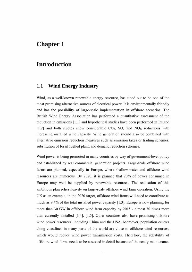
1) DFIG Topology
The AC/DC/AC converter connecting the rotor windings to the grid consists of two
voltage-source converters, i.e., rotor-side converter (RSC) and grid-side converter
(GSC), which are connected “back-to-back”, shown in Figure 1.1. Between the two
Chapter 1 Introduction 6
converters a DC-link capacitor is placed, as energy storage, in order to keep the
voltage variations (or ripple) in the DC-link voltage small. With the rotor-side
converter it is possible to control the shaft torque or the speed of the DFIG and also
the power factor at the stator terminals. The main objective for the grid-side
converter is to keep the DC-link voltage constant regardless of the magnitude and
direction of the rotor power. The grid-side converter works at the grid frequency
(with a controllable leading or lagging power factor in order to absorb or generate
reactive power). A transformer is often connected between the grid-side inverter or
the stator, and the grid. The rotor-side converter changes its output frequency,
depending on the wind speed.
IG
GB – Gearbox IG – Induction Generator
RSC – Rotor-Side Converter GSC – Grid-Side Converter
GB
Lchoke
Ps, Qs
RSC GSC Pr, Qr
Pc, Qc
Pm
Figure 1.1: Doubly-fed induction generator system and its power flows.
The back-to-back arrangement of the converters provides a mechanism of converting
the variable-voltage, variable-frequency output of the generator rotor winding (as its
speed changes) into a fixed-frequency, fixed-voltage output compliant with the grid.
The DC-link capacitance is an energy storage element that provides an energy buffer
between the generator and the grid.
The power electronic converters need only be rated to handle the rotor power which
is a fraction of the total power, typically about 30% nominal generator power.
Therefore, the losses in the power electronic converter can be reduced, compared to a
system where the converter has to handle the nominal generator power, and the
system cost is lower due to the partially rated power electronics.
At the current state of development, most DFIG power electronics utilise two-level
six-switch voltage-source conversion technology. The switching elements in these power

Chapter 1 Introduction 7
converters are likely to be insulated-gate bipolar transistors (IGBTs). The six-switch
converter can synthesise a three-phase output voltage which can be of arbitrary magnitude,
frequency and phase, within the constraint that the peak line voltage is less than the
DC-link voltage. The converter is capable of changing the output voltage almost
instantaneously – the limit is related to the switching frequency of the pulse-width
modulated switching devices, and delays introduced by any filtering on the output.
2) Power Flow
In steady-state at fixed turbine speed with a lossless DFIG system, the mechanical
power from the aerodynamic system is balanced by the DFIG power, in Figure 1.1,
Pm = Ps + Pr. It follows that
ssmss
rsmsmrmsmr sPsTTTTPPP −=−=⎟⎟
⎠
⎞⎜⎜⎝
⎛ −−=−=−= ωω
ωωωωω (1.1)
where s is defined as the slip of the generator: s
rssωωω −
= .
Therefore if the maximum slip is limited, say to 0.3, the rotor winding converters can
be rated as a fraction of the induction generator rated power. This is typically around
±30% for DFIG in wind power generation systems and gives a slip range of ±0.3.
From the above relationships, the stator and rotor power are Ps = Pm/(1–s) and Pr =
–sPm/(1–s), respectively. To assess the change in mechanical power during different
rotor speeds, the following analysis is carried out with all terms in per unit values.
The slip is assumed to vary from a sub-synchronous value of +0.35 to a
super-synchronous value of –0.35.
The per unit output power from wind turbine is
3__ puwindpupm VCP = (1.2)
Here we use the example wind turbine model in MATLAB (The Mathworks Inc.,
2008) [1.24]: λβλ
βλ λ643
21
5
),( ceccccC i
c
ip +⎟⎟
⎠
⎞⎜⎜⎝
⎛−−=
−
, 1
035.008.0
113 +
−+
=ββλλi
,

Chapter 1 Introduction 8
with the coefficients as c1 = 0.5176, c2 = 116, c3 = 0.4, c4 = 5, c5 = 21 and c6 = 0.0068.
wind
r
VRωλ = is the tip-speed ratio. The maximum value of Cp is 0.48 when β = 0 and λ
= 8.1. These are defined as base values for per unit calculations. Here base wind
speed is 12 ms−1, the gear ratio is 10, rotor radius is 5.16m.
When s = –0.2, Cp is 0.48 then Pm is 1.0 p.u. ideally. Hence for 2 pole-pair generator,
s
rssωωω −
= , spur −=1_ω , )1()1(751.612
16.55)1( 7 scssV
R
wind
r −=−=×
−==πωλ .
Then at the base wind speed, the expression of Pm in terms of slip s is
⎥⎥⎦
⎤
⎢⎢⎣
⎡−+⎟⎟
⎠
⎞⎜⎜⎝
⎛−==
−
)1(48.01
48.0 7642
1
5
sccecccC
P i
c
i
pm
λ
λ, 035.0
)1(11
7
−−
=sciλ
. (1.3)
The above analysis is performed in MATLAB programming to assess power flow.
This turbine model will be used throughout the thesis. Figure 1.2 shows how the
rotor and stator power vary as the rotor slip changes from sub- to super-synchronous
modes. The speed of the rotor has to change as wind speed changes in order to track
the maximum power point of the aerodynamic system given by the optimum
tip-speed ratio. Slip, s, therefore is related to incident wind speed. In this case, a slip
of –0.2 occurs with rated wind speed (12 ms−1). As wind speed drops, slip has to
increase and in this case has a maximum value of 0.35.
It is clear that the mechanical power, Pm, reaches its peak at super-synchronous speed
when s = –0.2. When rotating at the synchronous speed (s = 0), the DFIG supplies all
the power via the stator winding, with no active power flow in the rotor windings and
their associated converters. Note that at s = 0, the stator power is at maximum. As the
wind speed increases, the rotational speed must also increase to maintain optimum
tip-speed ratios. In such circumstances, the machine operates at super-synchronous
speeds (s < 0). The mechanical power flows to the grid through both the stator
windings and the rotor windings and their converter. At lower wind speeds, the
blades rotate at a sub-synchronous speed (s > 0). In such circumstances, the rotor
converter system will absorb power from the grid connection to provide excitation

Chapter 1 Introduction 9
for the rotor winding. With such a scheme it is possible to control the power
extracted from the aerodynamic system such that the blade operates at the optimum
aerodynamic efficiency (thereby extracting as much energy as possible) by adjusting
the speed of rotation according to the incident wind speed.
-0.4 -0.3 -0.2 -0.1 0 0.1 0.2 0.3 0.40.2
0.4
0.6
0.8
1
1.2P
m(p
.u.)
-0.4 -0.3 -0.2 -0.1 0 0.1 0.2 0.3 0.4-0.5
0
0.5
1
Ps(
p.u.
),Pr(p
.u.)
s
PsPr
Sub-synchronous Super-synchronous
Figure 1.2: DFIG mechanical power, generator stator power and rotor power in per unit (Pm, Ps, and
Pr) in respect to rotor slip s.
3) Rotor-Side Converter
The rotor-side converter applies the voltage to the rotor windings of the induction
generator for excitation. The purpose of the rotor-side converter is to control the rotor
currents such that the rotor flux position is optimally oriented with respect to the
stator flux in order that the desired torque is developed at the shaft of the machine.
The vector control for the generator can be embedded in an optimal power tracking
controller for maximum energy capture in a wind power application [1.8]. By
controlling the active power of the converter, it is possible to vary the rotational
speed of the generator, and thus the speed of the shaft of the wind turbine. This can
then be used to track the optimum tip-speed ratio as the incident wind speed changes
thereby extracting the maximum power.
The rotor-side converter uses a torque controller to regulate the wind turbine output
power measured at the machine stator terminals. The power is controlled in order to

Chapter 1 Introduction 10
follow a pre-defined turbine power-speed characteristic to track the maximum power
point. The actual electrical output power from the generator terminals, added to the
total power losses (mechanical and electrical) is compared with the reference power
obtained from the wind turbine characteristic.
The control scheme of the rotor-side converter is organised in a generic way with
two series of Proportional-Integral (PI) controllers. The reference q-axis rotor
current irqref can be obtained either from an outer speed-control loop or from a
reference torque. These two options may be termed a speed-control mode or
torque-control mode for the generator, instead of regulating the active power
directly. Another PI controller is included to produce a reference signal for the
d-axis rotor current component − irdref − to control the reactive power required from
the generator.
The reference rotor current irqref is forced in the rotor winding by the rotor-side
converter. The actual irq component of rotor current is compared with irqref and the
error is reduced to zero by a PI controller with the inner control loop. The output of
this current controller is the voltage vrq generated by the rotor-side converter. With
another similarly regulated ird and vrd component the required 3-phase voltages
applied to the rotor winding are obtained and force the ird and irq towards their
reference values.
In other words, the rotor-side converter provides a varying-frequency excitation
depending on the wind speed conditions. The induction generator is controlled in a
synchronously rotating dq-axis frame, with the d-axis oriented along the stator-flux
vector position in one common implementation. This is called stator-flux orientation
(SFO) vector control. Consequently, the active power and reactive power are
controlled independently from each other. Orientation frames applied in traditional
vector control of induction generators such as rotor-flux orientation and
magnetising-flux orientation, can also be utilised [1.25]. Additionally, the
stator-voltage orientation (SVO) is also commonly used in DFIG vector controllers
[1.9].

Chapter 1 Introduction 11
4) Grid-Side Converter
The grid-side converter aims to regulate the voltage of the DC-link capacitor.
Moreover, it can generate or absorb reactive power for voltage support. The
converter is also current regulated, with the d-axis current used to regulate the
DC-link voltage and the q-axis current component to regulate the reactive power. The
vector-control method uses a reference frame oriented along the stator voltage vector
position, enabling independent control of the active and reactive power flowing
between the grid and the converter. Therefore, the grid-side converter control has the
potential for optimising the grid integration with respect to steady-state operation
conditions, power quality and voltage stability.
The function is realised with two control loops as well. An outer regulation loop
consists of a DC voltage regulator. The output of the DC voltage regulator is a
reference current icdref for the current regulator. The inner current regulation loop
consists of a current regulator controlling the magnitude and phase of the voltage
generated by converter from the icdref produced by the DC voltage regulator and
specified q-axis reference icqref, which is used to control power factor.
5) DFIG Fault-Ride Through
Recently, research about DFIG systems focuses on its fault-ride through capability
during AC-side disturbances. The motivation for this is the grid codes which are now
requiring fault-ride through capability for renewable power integration. Appropriate
modelling of DFIG systems are analysed for different purposes such as for power
system stability analysis [1.26]-[1.28]. For grid integration, under AC-side voltage
dip conditions, the DFIG fault-ride through analysis is described in [1.29]-[1.33].
New fault tolerant DFIG topologies and control methods are proposed for the
systems [1.34]-[1.36]. More detailed analysis of DFIG fault conditions and converter
protection methods will be summarised in Chapter 2, with a new protection scheme
being proposed.

Chapter 1 Introduction 12
1.3.2 Permanent Magnet Synchronous Generators
The DFIG systems utilise a gearbox that couples the wind turbine to the generator.
The gearbox suffers from faults and requires regular maintenance. The reliability of
the variable-speed wind turbine system can be improved significantly by using a
direct-driven PMSG − eliminating the gearbox. With the development of high energy
magnet materials, the PMSG has received much attention in wind energy
applications because of their self-excitation. The use of permanent magnets in the
rotor of the PMSG makes it unnecessary to supply magnetising current. Hence,
because of the absence of the magnetising current PMSG solutions are often more
efficient than other machines. To extract maximum power from the fluctuating wind,
variable-speed operation of the wind-turbine PMSG is necessary. Two power
electronic topologies are proposed for variable-speed operation of PMSG. They
require different control strategies for the generator. PMSGs are also being used in
wind turbines with gearboxes, for example, Doosan Heavy Industries.
1) Large-Scale PMSG System
For this system, control strategies use wind velocity to determine the optimum shaft
speed, hence, the generator speed. For a general system, an anemometer-based
control strategy increases cost and may even reduce the reliability of the overall
system. However, for large wind turbines, the anemometer represents only a very
small fraction of the total cost and the control strategy based on wind velocity to
determine optimum generator speed is adopted. In [1.11], [1.12], the current vector
of an interior-type PMSG is controlled to optimise the wind-turbine operation at
various wind speed, which requires six active switches to be controlled, Figure 1.3.
VSI
PMSG Lchoke
C Grid
C
DC cable
VSC
MPPT PWM Vector Control Pitch Control
(−1 kV)
(+1 kV)
Figure 1.3: Large-scale PMSG power conversion system topology.

Chapter 1 Introduction 13
2) Small-Scale PMSG System
A control strategy for the generator-side converter (DC/DC boost converter) with
output maximisation of a PMSG small-scale wind turbine was developed in [1.13],
Figure 1.4. The generator-side switch-mode rectifier (a diode rectifier and boost
converter) is controlled to achieve maximum power from the wind. The method
requires only one active switching device (IGBT), which is used to control the
generator torque to extract maximum power. It is simple and a low-cost solution for a
small-scale wind turbine.
VSI Diode Rectifier
DC/DC BoostConverter
PMSG
L
Lchoke C Cf
DC cableGrid
MPPT PWM Vector Control Pitch Control
(+0.5 kV)
(−0.5 kV)
Figure 1.4: Small-scale PMSG power conversion system topology.
For a stand-alone system, the output voltage of the load side voltage-source inverter
(VSI) has to be controlled in terms of amplitude and frequency. Previous publications
related to PMSG-based variable-speed wind turbine mostly concentrate on grid
connected systems [1.37]-[1.39]. However, remote area local small-scale stand-alone
distributed generation system can utilise available renewable energy resources when
grid connection is not feasible. In [1.13], a control strategy is developed to control the
load voltage in a stand-alone mode. As there is no grid in a stand-alone system, the
amplitude and frequency of the output voltage has to be controlled. The load-side
pulse-width modulated (PWM) inverter uses a vector-control scheme to control the
amplitude and frequency of the output voltage. The stand-alone control is featured with
output voltage and frequency controller capable of handling variable load conditions.
Grid fault analysis of the PMSG system performance is discussed in [1.40], [1.41].
However, these are in terms of the grid disturbance conditions. Chapter 3 will deal
with the possible internal DC fault conditions of this wind power generation system.

Chapter 1 Introduction 14
1.4 Wind Power Collection and Transmission Technologies
Traditional alternating-current (AC) transmission and distribution systems are used
for integration of power generation and for long-distance power transmission and
distribution to power customers. There has been decades of operational experience
and it is mature in system operation and protection. However, since the increasing
integration of renewable power, there has been renewed interest in direct-current (DC)
transmission for offshore wind farm power collection and transmission, both
technically and economically [1.16]-[1.18]. For long-distance transmission and
offshore environments, DC transmission is more economic and may offer additional
technical benefits.
1.4.1 Collection Grid
Conventional offshore wind farms use AC systems. The wind farm “electrical
system” describes the electrical equipment and devices, including transformers,
cables/lines linking wind turbines and from them to platforms, and connecting
cables/lines from platforms to the shore. Offshore substation platforms may be
required in some cases for the transformers. In [1.42], the electrical system is defined
as: “basically all equipment required to deliver and control the electrical energy that
follows from the generator to the grid.”
For AC systems, the offshore linking cables and transformers are called collection
grids [1.43]-[1.45], or collector/collection systems [1.46], [1.47]. The collection grids
are always of a medium voltage (MV). While the transmission line to the grid are of
high voltage (HV) to improve transmission efficiency. Until now, there have been
many discussions about the transmission choices such as traditional high-voltage
alternative current (HVAC), conventional high-voltage direct current (HVDC), and
voltage-source converter based HVDC. This will influence the topology of the
collection grid due to different power conversion requirements. More detailed
collection grid topologies will be studied in Chapter 6 for redundancy analysis.

Chapter 1 Introduction 15
1.4.2 High-Voltage Direct-Current Transmission
The history of electric power systems began with DC transmission (1882, Thomas
Edison). However, it was quickly replaced by three-phase AC transmission because
of several advantages of the latter. The most distinct advantage of AC transmission is
that power can be transformed to different voltage level using transformers, which
allows efficient long-distance power transmission. In addition, circuit breakers for
alternating current can take advantage of the natural current zeros that occur twice
per cycle, and AC motors are cheaper and more robust than DC motors.
In spite of the prevailing use of AC transmission in power systems, interest in DC
transmission still remained. In 1954, the first commercial HVDC link between
mainland Sweden to Gotland island was commissioned. Since then, the installed
power of HVDC transmission systems worldwide has increased steadily, and recently
a dramatic increase in capacity has been initiated. Given the extra costs and losses
related to the converter stations, HVDC transmission is justified by some conditions
where the DC technology is the most appropriate or may be the only solution:
Underground Cable Power Transmission: Due to their physical structures, cables
have much higher capacitance than overhead lines. The capacitive current in cables
created by the alternating voltage makes AC power transmission over long-distance
cables inefficient [1.14]. If the power is transmitted by direct currents, there will be
no losses related to capacitive currents. Moreover, to transmit the same amount of
power, DC transmission needs fewer power lines than AC transmission. Accordingly,
the costs and losses of the converter stations are balanced by savings on the overhead
lines/cables where the break-even distance is around several hundred kilometres
depending on the project specifications.
Unsynchronised AC-System Connection: AC transmission is only possible if the
two interconnected AC systems operate synchronously. DC transmission does not
have such requirements and can be used to interconnect asynchronous systems.
Many back-to-back HVDC links have been built for such purposes [1.14], [1.15].
Chapter 1 Introduction 16
Power System Stability Improvement: One of the major features of the HVDC
technology is its capability to manipulate power flows in a very short time, which
can be utilised to improve the stability of the AC system [1.48].
Firewall Function: Large interconnected AC systems have many advantages,
such as the possibility to use larger and more economical power plants, reduction of
reserve capacity in the systems, utilisation of the most efficient energy resources, and
achieving an improved system reliability. However, larger interconnected AC
systems also increase the system complexity from the operational point of view. One
of the consequences of such complexity is the large blackouts in America and Europe
[1.48]. In this aspect, HVDC links have a “firewall” function in preventing cascaded
AC system outages.
1) HVDC Transmission Using Line-Commutated Current-Source Converters
Line-commutated converters based on thyristor are called current-source converters
(CSCs) [1.14]. The CSC can be used for transmitting power in two directions, i.e.,
the rectifier mode and the inverter mode. This is achieved by applying different firing
angles on the valves (theoretically 0°−90° for rectifier; 90°−180° for inverter). An
HVDC link is essentially constructed using two converters, which are interconnected
on the DC sides. The interconnection could be overhead lines, underground cables,
or a back-to-back connection. The application of CSC-HVDC technology has been
very successful. However, the CSC technology suffers from several inherent
weaknesses:
Consumption of Reactive Power: One problem is that the CSC always consumes
reactive power, either in rectifier mode or in inverter mode. Depending on the firing
angles, the reactive power consumption of a CSC-HVDC converter station is
approximately 50–60 % of the active power [1.48]. The reactive-power consumption
requires compensation by connecting large AC capacitors at the converter stations.
For a common CSC-HVDC link, the capacitors not only increase the costs, but also
occupy large amounts of space volume of the converter station. Besides, large
capacitors also contribute to the transient overvoltage and low-order harmonic
resonance problems of the HVDC link when connects to a weak AC system.

Chapter 1 Introduction 17
Commutation Failures: Another problem of the CSC-HVDC system is the
occurrence of commutation failures at the inverter station typically caused by
disturbances in the AC system [1.14]. The commutation failure creates a short circuit
on the DC side, which temporarily stops the power transmission. Commutation
failures are less common phenomena than in the early schemes owing to the vastly
improved solid state valve technology that exist nowadays.
Weak AC-System Connection: This problem can become a limiting factor for
CSC-HVDC applications. For CSCs, the successful commutation of the alternating
current from one valve to the next relies on the stiffness of the alternating voltage,
i.e., the network strength of the AC system [1.48]. If the AC system has low
short-circuit capacity relative to the power rating of the HVDC link, i.e., low
short-circuit ratio (SCR), more problematic interactions between the AC and the DC
systems are expected. Besides, the SCR of the AC system also imposes an upper
limitation on the HVDC power transmission.
2) HVDC Transmission Using Force-Commutated Voltage-Source Converters
The voltage-source converter (VSC) is a relatively new converter technology for
HVDC transmission. The first commercial VSC-HVDC (HVDC-Light) link with a
rating of 50 MW was commissioned in 1999 at Gotland Island, Sweden, close to
the world’s first CSC-HVDC link [1.17]. Voltage-source converters utilise
self-commutating switches, gate turn-off thyristors (GTOs) or insulated-gate
bipolar transistors (IGBTs), which can be actively turned-on and -off. Therefore, a
VSC can produce its own sinusoidal voltage waveform using pulse-width
modulation (PWM) technology independent of the AC system. Many different
topologies have been proposed for VSCs. For HVDC applications, three major
types are favoured: the two-level converter, the multi-level converter, and the
modular multi-level converter.
The two-level bridge is the simplest topology to construct a three-phase
force-commutated VSC. The bridge consists of six switches with associated
anti-parallel diodes. For an HVDC link, two VSCs are interconnected on the DC
sides. For high-voltage applications, series connection of switching devices is
Chapter 1 Introduction 18
necessary. The operation principle of the two-level bridge is simple. Each phase of
the VSC can be connected either to the positive DC terminal, or the negative DC
terminal. By adjusting the width of pulses, the output voltage can be produced to
interface with the grid voltage after filtering by phase reactors and shunt filters.
Multi-level VSCs are promising for medium- and high-power conversion
applications [1.49]-[1.51]. There are two common multi-level converters: three-level
neutral-point-clamped (3L-NPC) converter and five-level flying capacitor (5L-FC)
converter. The key components that distinguish the 3L-NPC topology from the
two-level converter are the two clamping diodes in each phase. These two diodes
clamp the switch voltage to half of the DC-link voltage. Thus, each phase of the VSC
can switch to three different voltage levels, i.e., the positive DC terminal, the
negative DC terminal and zero volts (the mid-point). Consequently, voltage pulses
produced by a multi-level VSC are a closer match to the reference voltage. Therefore,
the multi-level converter has less harmonic content. Additionally, they have lower
switching losses. Compared to two-level VSCs, 3L-NPC VSCs require more diodes
for neutral-point clamping. However, the total number of switching components does
not necessarily have to be higher [1.48]. The NPC concept can be extended to higher
number of voltage levels, which can result in further improved harmonic reduction
and lower switching losses. However, for high-voltage converter applications, the
neutral-clamped diodes complicate the insulation and cooling design of the converter
switches [1.48].
The recently proposed modular multi-level converter (MMC) concept has attracted
interest [1.50]. Compared to the above two topologies, one major feature of the MMC
is that no common capacitor is connected at the DC side. The DC capacitors are
distributed into each module, while the converter is built up by cascade-connected
modules. The MMC concept is especially attractive for high-voltage applications,
since the converter can be easily scaled up by inserting additional modules in each arm.
If considerable numbers of modules are cascaded (approximately 100 modules would
be typical for HVDC applications), each module theoretically only need to switch on
and off once per period, which greatly reduces the switching losses. With only five
modules, the waveform already resembles much better the sinusoidal voltage reference
than the other two topologies. With MMC, the harmonic content of the voltage
Chapter 1 Introduction 19
produced by the VSC is so low that additional filtering equipment is almost
unnecessary. An additional benefit of the MMC is that the control system has an extra
freedom in dealing with faults at the DC side. The DC capacitors are not necessarily
discharged during faults. Thus, the fault recovery can be faster.
Compared to the other two topologies, the major drawback of the MMC topology is
that the required switching components are doubled since only one of the switches of
each module contributes to the phase voltage. In addition, the design and control of
the MMC are generally more complex than the two-level converter. On the other
hand, the reduction of switching losses and savings on filtering equipment of the
MMC may eventually justify its application for HVDC transmission.
The VSC can generally be treated as an ideal voltage source where the control
system has the freedom to specify the magnitude, phase, and frequency of the voltage
waveform. However, for control design and stability analysis, it is important to take
into account the limitation of the converter in terms of active and reactive power
transfer capability. One such limit is the converter current limitation, which is
imposed by the current carrying capability of the VSC switches since both the active
power and the reactive power contribute to the current flowing through the switches.
Accordingly, if the converter is intended to support the AC system with reactive
power supply or consumption, the maximum active power has to be limited to make
sure that the switch current is within the limit.
Another limitation which determines the reactive-power capability of the VSC is the
maximum and minimum voltage magnitudes that the VSC can produce (modulation
index limitation). The overvoltage limitation is imposed by the DC-link voltage of
the VSC. The under-voltage limit, however, is limited by the main-circuit design and
the active power transfer capability, which requires a minimum voltage magnitude to
transmit the active power.
VSC-HVDC technology overcomes most of the weakness of the CSC-HVDC
technology. In addition, it supports the AC system with reactive power. Similar to a
CSC-HVDC system, a VSC-HVDC system can quickly run up or run back the active
power for AC system emergency power support.

Chapter 1 Introduction 20
Besides the above features, the most essential one is that a VSC-HVDC system has
an advantageous connection capability with AC systems, i.e., with properly designed
control systems, VSC-HVDC system has the potential to be connected to any kind of
AC system with any number of links [1.52], [1.53]. This outstanding feature will
eventually bring the DC transmission technology to ever broader application fields.
Multi-terminal VSC-HVDC connection applications for wind power integration are
gaining more research effort [1.18], [1.54]-[1.57]. With multi-terminal connections to
different onshore grids, the integration of large-scale offshore wind farms and
possible multiple weak AC system connections are possible. This is also the
application background of the work reported in Chapter 4 and 5.
1.5 Protection Development of DC Systems
Fault vulnerability is one of the most significant issues that constrain the
development of voltage-source converter based DC networks, especially in
high-power scenarios. In addition, this is due to the lack of mature commercial DC
switchgear products. However, as introduced above, VSC-HVDC power
transmission provides greater operational flexibility which suits renewable energy
sources. One typical application is for large-scale offshore wind farm integration to
utility grids [1.16], [1.18], [1.58], [1.59] where a reliable DC network is a
prerequisite.
In such systems, cable faults do occur more frequently compared with other parts of
the system. The most common reason for cable fault is insulation deterioration and
breakdown. There can be several causes [1.60]: physical damage (the most serious
short-circuit fault can occur because of this); environmental stresses such as damp,
especially at the junctions of cables, where the cabling system is exposed to soil or
water; electrical stresses due to overload operation or operation at high temperature;
and cable aging. These factors can all lead to a ground fault. There has been limited
discussion about the influence of DC faults on DC networks at transmission and
distribution levels. The following aspects regarding DC system fault analysis have
been reported:

Chapter 1 Introduction 21
1) Line-Commutated, Current-Source Converter HVDC Systems
Conventional line-commutated CSC-based HVDC transmission systems are robust to
DC fault overcurrents because of their current-regulated nature [1.61]. DC voltage
change is used for fault detection. Since the application of line-commutated
CSC-HVDC systems, the overvoltage phenomenon of this current-regulated DC
system has been discussed [1.62]-[1.64]. Recently, HVDC protection research has
been focused on specific cable fault location approaches. Protection coordination is
seldom studied because of the lack of development in multi-terminal DC networks.
2) Cable Fault Location Techniques
At the current stage, cable fault location research is focused on offline techniques
[1.65]-[1.69]. Techniques widely used in industry are commonly time-consuming
trace methods using acoustic or electromagnetic approaches [1.65]. Travelling
wave based methods have also been researched using different algorithms
[1.66]-[1.69]. They utilise a travelling wave model of the cable for overvoltage
transient analysis and location. A high-frequency pulse wave is injected into the
faulty cable and the fault location is found by the comparison between the original
and reflected waves. However, when the system structure is complex (e.g. meshed
for multi-terminal connection) the DC bus will experience multiple reflections
which will influence location results. A detailed cable model is required for
accurate fault location using the transient response to a high-frequency pulse. For
AC network and line-commutated CSC-HVDC, these offline methods are adequate
because fast fault location may not be critical. However, for VSC-based HVDC
systems, a fast and accurate fault location is required for effective operation of
protective devices [1.70].
3) VSC under AC-Side Faults
VSCs are widely used as rectifiers or inverters for electrical power conversion. If
each conversion element of a DC wind farm is a VSC, the VSC control can cope
with grid-side AC disturbances, during which appropriate control and protection
methods can be used to protect its power electronic devices [1.71], [1.72]. The short
circuit current contribution of VSC-HVDC systems for AC system faults are also

Chapter 1 Introduction 22
analysed in respect of AC system protection. It is shown that the VSC-HVDC system
may contribute short-circuit current determined by the SCR [1.73].
4) VSC Internal Faults
In terms of fault-tolerant VSCs, the research aims are to protect the system from
possible IGBT faults (e.g. short-circuits) where there are many opportunities to
allocate backup function or include redundant devices [1.74]-[1.77].
In terms of DC network faults, with parallel connected VSCs, severe overcurrents
due to discharge of the DC-link capacitances are a major issue: the converters’ power
electronic devices, particularly the freewheel diodes, are subject to overcurrent with
DC-side faults on cables or buses. The overcurrents eventually flow through the
freewheel diodes in the basic converter configuration and the converter is defenceless
against such DC-side faults, such as a DC-link short-circuit, DC cable short-circuits
and DC cable ground faults. These fault conditions need to be analysed and
simulated in detail for effective system protection prior to the development of
practical high-power VSC-HVDC networks. Relevant works are now summarised:
VSC-Based DC Distribution Systems: For DC distribution networks with VSCs,
the following research has been reported: 1) fault simulation of a DC micro-grid and
switchgear/fuse allocation [1.78]; 2) fault analysis of a VSC-based DC distribution
system for a shipboard application [1.79], [1.80] − by replacing diodes with
controllable gate power electronic devices to provide bi-directional current blocking
function; 3) dedicated discharge overcurrent protection for DC-link capacitors [1.80],
[1.81]. However, these studies are for low-power DC distribution systems and cannot
be applied to high-power transmission systems.
VSC-HVDC Systems: Fault detection and location for meshed VSC-HVDC
systems is discussed in [1.82], [1.83] at the transmission level. The technique in
[1.84] extracts the fault signature by comparing initial current change, the current
rise time interval, or current oscillation pattern at different switch locations. Based on
this technique, [1.83] proposes a fault location and isolation method. This is mainly
based on AC-side circuit breakers, and no DC switchgear configuration is discussed
due to cost considerations. VSC-HVDC DC cable overvoltage protection under

Chapter 1 Introduction 23
line-to-ground faults is analysed in [1.84]. However, the protection scheme is not
designed specifically for overcurrents flowing through power electronic devices,
which are the most vulnerable devices of the system.
Most of the research reported on DC fault analysis with VSC configurations are
based on numerical simulations without a theoretical basis through circuit analysis.
There is no detailed analysis of the overcurrent during the fault. Moreover, the speed
requirement for DC circuit breakers can only be configured after identifying critical
time limits under various fault conditions. AC-side switchgear is not considered fast
enough to cope with the rapid rise of fault current characteristic of freewheel diode
conduction which can damage power electronic devices in several milliseconds.
In addition, most work focuses on the DC short-circuit faults at the DC rails [1.80].
However, fault analysis in VSC-based DC networks and DC cable faults is seldom
reported, but a cable short-circuit fault is potentially more common than a DC rail
fault and the impact of a DC cable fault on the freewheel diodes in the VSC can be
worse than that of a direct DC rail short circuit due to the inductive component in the
discharge path. This problem will be discussed in Chapter 4. Although underground
cables are seldom short-circuited in comparison to overhead lines, it is a critical
condition and needs to be analysed particularly for switchgear relay and protection
design. In contrast, ground faults are more common but less serious. However,
accurate fault location for effective protection coordination is required for
high-impedance ground faults – this is also addressed in Chapter 4. This protection
coordination will be designed for a large-scale meshed wind farm system in Chapter
5. In terms of wind farm topology redundancy, the analysis in Chapter 6 aims at
enhancing reliability whilst considering economic costs.
1.6 Outline of Thesis
This thesis is presented in the following chapters:
Chapter 2 – The protection schemes for the DFIG system are introduced. A novel
protection circuit based on series dynamic resistors for the rotor-side converter is
proposed after detailed analysis of the rotor overcurrent under various fault
Chapter 1 Introduction 24
conditions. This protection scheme is advantageous particularly for asymmetrical
AC-side fault conditions. During such faults, the traditional crowbar protection
circuit results in reactive power absorption that deteriorates the grid voltage recovery.
The proposed protection system can shorten the time of crowbar operation to
minimise reactive power consumption.
Chapter 3 – The PMSG-based wind power generation system protection is presented
in this chapter. For large-scale systems, a voltage-source converter rectifier is
included; for small-scale systems, a boost circuit is used. Protection circuits for these
topologies are studied with simulation results for different fault conditions. These
electrical protection methods are all in terms of dumping redundant energy resulting
from disrupted path of power delivery. Pitch control of large-scale wind turbines are
considered for effectively reducing rotor shaft overspeed.
Chapter 4 – A radial VSC-based DC network for wind farm connection is presented
in this chapter. Detailed analysis of this DC system is performed under both
short-circuit and ground fault conditions. The critical stages of the progress of the
fault are defined for this nonlinear system and these are used to coordinate the
protection. Simulation results are used to assess a relay coordination methodology
for this system. A ground fault location method is presented and tested under
different ground resistances, distances, and operating conditions.
Chapter 5 – Large-scale wind farm collection and transmission systems may
potentially utilise a meshed connection to enhance reliability. However, for
voltage-source converter based HVDC systems, a meshed network leads to a
complex protection coordination strategy. With allocation of economical
uni-directional power electronic DC circuit breakers, this chapter presents a
protection methodology for this large-scale system. DC bus faults are dealt with in
particular due to the complex multi-terminal topology of this large-scale DC system.
Chapter 6 – Redundancy analysis for the wind farm collection and transmission
systems is carried out based on economic statistics of an existing UK wind farm
project. Equipment investment and economic operational losses are compared
resulting in a balance between the technical performance and economic investment.
Chapter 1 Introduction 25
A redundancy design method is proposed to achieve an optimal degree of
redundancy using reliability economic loss statistics.
Chapter 7 – A summary of the key research outcomes and contributions of the thesis
is provided along with conclusions of the work and suggestions for future research.
1.7 List of Publications
This thesis has resulted in the following publications:
A. Refereed Journal Papers
[J1] J. Yang, J. E. Fletcher, and J. O’Reilly, “Short-circuit and ground fault analysis and location in VSC-based DC network cables,” IEEE Transactions on Industrial Electronics, invitation from the 2010 ISIE conference for special section publication, submitted, Dec. 2010.
[J2] J. Yang, J. E. Fletcher, and J. O’Reilly, “Protection of meshed VSC-HVDC transmission systems for large-scale wind farms,” IET Renewable Power Generation, submitted, Dec. 2010.
[J3] J. Yang, J. E. Fletcher, and J. O’Reilly, “Multi-terminal DC wind farm collection grid internal fault analysis and protection design,” IEEE Transactions on Power Delivery, vol. 25, no. 4, pp. 2308-2318, Oct. 2010.
[J4] J. Yang, J. E. Fletcher, and J. O’Reilly, “A series-dynamic-resistor-based converter protection scheme for doubly-fed induction generator during various fault conditions,” IEEE Transactions on Energy Conversion, vol. 25, no. 2, pp. 422-432, Jun. 2010.
[J5] J. Yang, J. O’Reilly, and J. E. Fletcher, “Reliability enhancement of offshore wind farms by redundancy analysis,” Journal of Automation of Electric Power Systems, vol. 34, no. 4, pp. 84-91, Feb. 2010.
B. Book Chapter
[B1] J. E. Fletcher and J. Yang, “Introduction to doubly-fed induction generator for wind power applications,” Sustainable Energy, 978-953-7619-X-X, Oct. 2010.
C. Refereed Conference Papers
[C1] J. Yang, J. E. Fletcher, and J. O’Reilly, “An overview on DC cable modelling for fault analysis of VSC-HVDC transmission systems,” Australasian Universities

Chapter 1 Introduction 26
Power Engineering Conference, AUPEC 2010, Christchurch, New Zealand, 5-8 Dec. 2010.
[C2] J. Yang, J. E. Fletcher, and J. O’Reilly, “Protection scheme design for meshed VSC-HVDC transmission systems for large-scale wind farms,” the 9th International Conference on AC and DC Power Transmission, IET ACDC 2010, London, UK, 20-21 Oct. 2010.
[C3] J. Yang, J. E. Fletcher, and J. O’Reilly, “Multi-terminal DC wind farm collection grid internal fault analysis,” IEEE International Symposium on Industrial Electronics ISIE 2010, Bari, Italy, 4-7 Jul. 2010.
[C4] J. Yang, Y. Gao, and J. O’Reilly, “Permanent magnet synchronous generator converter protection analysis during DC wind farm open-circuit fault condition,” The 9th IEEE Annual Electrical Power and Energy Conference 2009, Montreal, Quebec, Canada, 22-23 Oct. 2009.
[C5] J. Yang, J. E. Fletcher, and J. O’Reilly, “A series dynamic resistor based converter protection scheme for doubly-fed induction generator during various fault conditions,” IEEE Power & Energy Society General Meeting 2009, Calgary, Alberta, Canada, 26-30 Jul. 2009.
[C6] J. Yang, J. O’Reilly, and J. E. Fletcher, “Protection scheme switch-timing for doubly-fed induction generator during fault conditions,” IEEE PowerTech 2009, Bucharest, Romania, 28 Jun. – 2 Jul. 2009.
[C7] J. Yang, J. O’Reilly, and J. E. Fletcher, “Redundancy analysis of offshore wind farm collection and transmission systems,” The 1st International Conference on SUPERGEN, Nanjing, China, 6-7 Apr. 2009.
[C8] J. Yang, D. G. Dorrell, and J. E. Fletcher, “Fault ride-through of doubly-fed induction generator with converter protection schemes,” IEEE International Conference on Sustainable Energy Technologies, Singapore, 24-27 Nov. 2008.
[C9] J. Yang, D. G. Dorrell, and J. E. Fletcher, “A new converter protection scheme for doubly-fed induction generators during disturbances,” The 34th Annual Conference of the IEEE Industrial Electronics Society, Orlando, Florida, USA, 10-13 Nov. 2008.
D. Non-refereed Conference Papers, Seminar Papers
[N1] J. Yang, “PSCAD/EMTDC simulations for wind farm transient analysis and protection scheme design,” Flux Users Conference, Autrans, France, 21-23 Oct. 2009.
Chapter 1 Introduction 27
1.8 References
[1.1] British Wind Energy Association. UK Wind Energy Database (UKWED). Available: http://www.bwea.com/ukwed/index.asp, 2010.
[1.2] E. Denny and M. O’Malley, “Wind generation, power system operation, and emissions reduction,” IEEE Trans. Power Syst., vol. 21, no. 1, pp. 341-347, Feb. 2006.
[1.3] British Wind Energy Association. Offshore Wind. Available: http://www.bwea.com/offshore/index.html, 2010.
[1.4] The European Wind Energy Association. European Statistics. Available: http://www.ewea.org/index.php?id=1486, 2010.
[1.5] The European Wind Energy Association. Offshore Statistics. Available: http://www.ewea.org/index.php?id=1861, 2010.
[1.6] P. J. Tavner, J. Xiang, and F. Spinato, “Reliability analysis for wind turbines,” Wind Energy, vol. 10, pp. 1-18, Available: http://onlinelibrary.wiley.com/doi/10.1002/we.204/pdf, 2007.
[1.7] British Wind Energy Association, Stage 3 Discussion Document – GB Electricity Network Access. Available: http://www.bwea.com/pdf/pathtopower/Stage3.pdf, Mar. 2006.
[1.8] R. Pena, J. C. Clare, and G. M. Asher, “Doubly fed induction generator using back-to-back PWM converters and its application to variable-speed wind-energy generation,” IEE Proc.-Electr. Power Appl., vol. 143, no. 3, pp. 231-241, May 1996.
[1.9] S. Muller, M. Deicke, and R.W. De Doncker, “Doubly fed induction generator systems for wind turbines,” IEEE Ind. Appl. Mag., vol., no., pp. 26-33, May/Jun. 2002.
[1.10] Z. Chen, J. M. Guerrero, and F. Blaabjerg, “A review of the state of the art of power electronics for wind turbines,” IEEE Trans. Power Electron., vol. 24, no. 8, pp. 1859-1875, Aug. 2009.
[1.11] Z. Chen and E. Spooner, “Grid interface options for variable-speed, permanent-magnet generators,” IEE Proc.-Electr. Power Appl., vol. 145, no. 4, pp. 273-283, Jul. 1998.
[1.12] M. Chinchilla, S. Arnaltes, and J. C. Burgos, “Control of permanent magnet generators applied to variable-speed wind-energy systems connected to the grid,” IEEE Trans. Energy Convers., vol. 21, no. 1, pp. 130-135, Mar. 2006.
[1.13] M. E. Haque, M. Negnevitsky, and K. M. Muttaqi, “A novel control strategy for a

Chapter 1 Introduction 28
variable-speed wind turbine with a permanent-magnet synchronous generator,” IEEE Trans. Ind. Appl., vol. 46, no. 1, pp. 331-339, Jan./Feb. 2010.
[1.14] J. Arrillaga, High Voltage Direct Current Transmission, 2nd Edition. London: The Institution of Electrical Engineers, 1998.
[1.15] M. Bahrman and B. Johnson, “The ABCs of HVDC transmission technologies,” IEEE Power Energy Mag., vol. 5, no. 2, pp. 32-44, Mar./Apr. 2007.
[1.16] P. Bresesti, W. L. Kling, R. L. Hendriks, and R. Vailati, “HVDC connection of offshore wind farms to the transmission system,” IEEE Trans. Energy Convers., vol. 22, no. 1, pp. 37-43, Mar. 2007.
[1.17] N. Flourentzou, V. G. Agelidis, and G. D. Demetriades, “VSC-based HVDC power transmission systems: an overview,” IEEE Trans. Power Electron., vol. 24, no. 3, pp. 592-602, Mar. 2009.
[1.18] D. Jovcic and N. Strachan, “Offshore wind farm with centralised power conversion and DC interconnection,” IET Gener. Transm. & Distrib., vol. 3, no. 6, pp. 586-595, Jun. 2009.
[1.19] J. Rodriguez, J.-S. Lai, and F. Z. Peng, “Multilevel inverters: a survey of topologies, controls, and applications,” IEEE Trans. Ind. Electron., vol. 49, no. 4, pp. 724-738, Aug. 2002.
[1.20] B. Gemmell, J. Dorn, D. Retzmann, and D. Soerangr, “Prospects of multilevel VSC technologies for power transmission,” in Proc. IEEE/PES T&D Conf. Expo., pp. 1-16., Apr. 21-24, 2008.
[1.21] G. P. Adam, O. Anaya-Lara, G. M. Burt, D. Telford, B. W. Williams, and J. R. McDonald, “Modular multilevel inverter: pulse width modulation and capacitor balancing technique,” IET Power Electron., vol. 3, no. 5, pp. 702-715, Oct. 2010.
[1.22] S. Kouro, M. Malinowski, K. Gopakumar, J. Pou, L. G. Franquelo, B. Wu, J. Rodriguez, M. A. Perez, and J. I. Leon, “Recent advances and industrial applications of multilevel converters,” IEEE Trans. Ind. Electron., vol. 57, no. 8, pp. 2553-2580, Aug. 2010.
[1.23] J. Ribrant and L. M. Bertling, “Survey of failures in wind power systems with focus on Swedish wind power plants during 1997−2005,” IEEE Trans. on Energy Convers., vol. 22, no. 1, pp. 167-173, Mar. 2007.
[1.24] The Mathworks Inc., MATLAB (R2008a), Product Help, 2008.
[1.25] P. Vas, Vector Control of AC Machines, Oxford University Press, Oxford, UK, 1990.
[1.26] P. Ledesma and J. Usaola, “Doubly fed induction generator model for transient stability analysis,” IEEE Trans. Energy Conver., vol. 20, no. 2, pp. 388-397, Jun. 2005.

Chapter 1 Introduction 29
[1.27] A. Petersson, Analysis, modeling and control of doubly-fed induction generators for wind turbines, Ph.D. Thesis, Chalmers University of Technology, Goteborg, Sweden, 2005.
[1.28] I. Erlich, J. Kretschmann, J. Fortmann, S. Mueller-Engelhardt, and H. Wrede, “Modeling of wind turbines based on doubly-fed induction generators for power system stability studies,” IEEE Trans. Power Syst., vol. 22, no. 3, pp. 909-919, Aug. 2007.
[1.29] M. S. Vicatos and J. A. Tegopoulos, “Transient state analysis of a doubly-fed induction generator under three phase short circuit,” IEEE Trans. Energy Convers., vol. 6, no. 1, pp. 62-68, Mar. 1991.
[1.30] J. Morren, and S.W.H. de Haan, “Ridethrough of wind turbines with doubly-fed induction generator during a voltage dip,” IEEE Trans. Energy Convers., vol. 20, no. 2, pp. 435-441, Jun. 2005.
[1.31] J. Morren and S. W. H. de Haan, “Short-circuit current of wind turbines with doubly fed induction generator,” IEEE Trans. Energy Convers., vol. 22, no. 1, pp. 174-180, Mar. 2007.
[1.32] J. López, P. Sanchis, X. Roboam, and L. Marroyo, “Dyanmic behavior of the doubly fed induction generator during three-phase voltage dips,” IEEE Trans. Energy Convers., vol. 22, no. 3, pp. 709-717, Sep. 2007.
[1.33] J. López, E. Gubía, P. Sanchis, X. Roboam, and L. Marroyo, “Wind turbines based on doubly fed induction generator under asymmetrical voltage dips,” IEEE Trans. Energy Convers., vol. 23, no. 1, pp. 321-330, Mar. 2008.
[1.34] D. Xiang, R. Li, P. J. Tavner, and S. Yang, “Control of a doubly fed induction generator in a wind turbine during grid fault ride-through,” IEEE Trans. Energy Convers., vol. 21, no. 3, pp. 652-662, Sep. 2006.
[1.35] I. Erlich, H. Wrede, and C. Feltes, “Dynamic behavior of DFIG-based wind turbines during grid faults,” in Proc. Power Convers. Conf., Nagoya, Japan, Apr. 2-5, 2007.
[1.36] P. S. Flannery and G. Venkataramanan, “A fault tolerant doubly fed induction generator wind turbine using a parallel grid side rectifier and series grid side converter,” IEEE Trans. Power Electron., vol. 23, no. 3, pp. 1126-1135, May 2008.
[1.37] K. Tan and S. Islam, “Optimal control strategies in energy conversion of PMSG wind turbine system without mechanical sensors,” IEEE Trans. Energy Convers., vol. 19, no. 2, pp. 392-399, Jun. 2004.
[1.38] S. Morimoto, H. Nakayama, M. Sanada, and Y. Takeda, “Sensorless output maximization control for variable-speed wind generation system using IPMSG,” IEEE Trans. Ind. Appl., vol. 41, no. 1, pp. 60-67, Jan. 2005.
[1.39] P. Tenca, A. A. Rockhill, and T. A. Lipo, “Wind turbine current-source converter
Chapter 1 Introduction 30
providing reactive power control and reduced harmonics,” IEEE Trans. Ind. Appl., vol. 43, no. 4, pp. 1050-1060, Jul./Aug. 2007.
[1.40] A. Abedini and A. Nasiri, “PMSG wind turbine performance analysis during short circuit faults,” in Proc. IEEE Canada Electrical Power Conf., Montreal, Quebec, Canada, 25-26 Oct. 2007.
[1.41] A. D. Hansen and G. Michalke, “Multi-pole permanent magnet synchronous generator wind turbines’ grid support capability in uninterrupted operation during grid faults,” IET Renew. Power Gener., vol. 3, no. 3, pp. 333-348, May 2009.
[1.42] J. Ribrant, Reliability performance and maintenance – a survey of failures in wind power systems, M.Sc. Thesis. KTH School of Electrical Engineering, Stockholm, Sweden, Apr. 2006.
[1.43] B. Franken, H. Breder, M. Dahlgren, and E. K. Nielsen, “Collection grid topologies for off-shore wind parks,” 18th International Conference on Electricity Distribution, CIRED, Turin, Italy, Jun. 6-9, 2005.
[1.44] A. Sannino, H. Breder, and E. K. Nielsen, “Reliability of collection grids for large offshore wind parks,” 9th International Conference on Probabilistic Methods Applied to Power Systems, PMAPS, KTH, Stockholm, Sweden, Jun. 11-15, 2006.
[1.45] L. Liljestrand, A. Sannino, H. Breder, and S. Thorburn, “Transients in collection grids of large offshore wind parks,” Wind Energy, Wiley Interscience, Jul. 2007, online http://doi.wiley.com/10.1002/we.233
[1.46] R. A. Walling and T. Ruddy, “Economic optimization of offshore wind farm substations and collection systems,” 5th International Workshop on Large-Scale Integration of Wind Power and Transmission Networks for Offshore wind Farms, Glasgow, UK, Apr. 7-8, 2005.
[1.47] G. Quinonez-Varela, G. W. Ault, O. Anaya-Lara, and J. R. McDonald, “Electrical collector system options for large offshore wind farms,” IET Renew. Power Gener., vol. 1, no. 2, pp. 107-114, Jun. 2007.
[1.48] L. Zhang, Modeling and control of VSC-HVDC Links connected to weak AC systems, Ph.D. Thesis, Royal Institute of Technology, Stockholm, Sweden, 2010.
[1.49] J. Rodriguez, J.-S. Lai, and F. Z. Peng, “Multilevel inverters: a survey of topologies, controls, and applications,” IEEE Trans. Ind. Electron., vol. 49, no. 4, pp. 724-738, Aug. 2002.
[1.50] S. Kouro, M. Malinowski, K. Gopakumar, J. Pou, L. G. Franquelo, B. Wu, J. Rodriguez, M. A. Perez, and J. I. Leon, “Recent advances and industrial applications of multilevel converters,” IEEE Trans. Ind. Electron., vol. 57, no. 8, pp. 2553-2580, Aug. 2010.
[1.51] H. Abu-Rub, J. Holtz, J. Rodriguez, and B. Ge, “Medium-voltage multilevel converters – state of the art, challenges, and requirements in industrial
Chapter 1 Introduction 31
applications,” IEEE Trans. Ind. Electron., vol. 57, no. 8, pp. 2581-2596, Aug. 2010.
[1.52] M. Durrant, H. Werner, and K. Abbott, “Model of a VSC HVDC terminal attached to a weak ac system,” in IEEE Conf. Control Appl., Istanbul, 2003.
[1.53] L. Zhang, L. Harnefors and H.-P. Nee, “Interconnection of two very weak ac systems by VSC-HVDC links using power-synchronization control”, IEEE Trans. Power Systems, online early access, 2010.
[1.54] W. Lu and B. T. Ooi, “Multiterminal LVDC system for optimal acquisition of power in wind-farm using induction generators,” IEEE Trans. Power Electron., vol. 17, no. 4, pp. 558-563, Jul. 2002.
[1.55] W. Lu and B. T. Ooi, “Optimal acquisition and aggregation of offshore wind power by multiterminal voltage-source HVDC,” IEEE Trans. Power Del., vol. 18, no. 1, pp. 201-206, Jan. 2003.
[1.56] G. P. Adam, O. Anaya-Lara, and G. Burt, “Multi-terminal dc transmission system based on modular multilevel converter,” in Proc. 44th Int. Universities Power Eng. Conf., Glasgow, UK, Sept. 1-4, 2009.
[1.57] D. Jovcic, and B. T. Ooi, “Developing dc transmission networks using dc transformers,” IEEE Trans. Power Del., vol. 25, no. 4, pp. 2535-2543, Oct. 2010.
[1.58] C. Meyer, M. Hoing, A. Peterson, and R.W. De Doncker, “Control and design of DC grids for offshore wind farms,” IEEE Trans. Ind. Appl., vol. 43, no. 6, pp. 1475-1482, Nov./Dec. 2007.
[1.59] A. Prasai, J. S. Yim, D. Divan, A. Bendre, and S. K. Sul, “A new architecture for offshore wind farms,” IEEE Trans. Power Electron., vol. 23, no. 3, pp. 1198-1204, May 2008.
[1.60] M. J. Mousavi and K. L. Butler-Purry, “A novel condition assessment system for underground distribution applications,” IEEE Trans. Power Sys., vol. 24, no. 3, pp. 115-1125, Aug. 2009.
[1.61] P. M. Anderson, Power system protection. New York: IEEE Press, 1999.
[1.62] N. G. Hingorani, “Transient overvoltage on a bipolar HVDC overhead line caused by dc line faults,” IEEE Trans. Power Appar. Sys., vol. PAS-89, no. 4, pp. 592-610, Apr. 1970.
[1.63] E. W. Kimbark, “Transient overvoltages caused by monopolar ground fault on bipolar dc line: theory and simulation,” IEEE Trans. Power Appar. Sys., vol. PAS-89, no. 4, pp. 584-592, Apr. 1970.
[1.64] G. T. Wrate, I. K. Tasinga, S. S. Low, D. J. Melvold, R. S. Thallam, D. W. Gerlach, and J. Y. Chang, “Transient overvoltages on a three terminal dc transmission system due to monopolar ground faults,” IEEE Trans. Power Del., vol. 5, no. 2, pp. 1047-1053, Apr. 1990.

Chapter 1 Introduction 32
[1.65] E. C. Bascom, “Computerized underground cable fault location expertise,” in Proc. IEEE Power Eng. Soc. General Meeting, pp. 376-382, Apr. 10-15, 1994.
[1.66] X. Liu, A. H. Osman, and O. P. Malik, “Hybrid travelling wave/boundary protection for monopolar HVDC line,” IEEE Trans. Power Del., vol. 24, no. 2, pp. 569-578, Apr. 2009.
[1.67] Y.-J. Kwon, S.-H. Kang, D.-G. Lee, and H.-K. Kim, “Fault location algorithm based on cross correlation method for HVDC cable lines,” IET 9th Int. Conf. Developments in Power Syst. Protection, Glasgow, U.K., 17-20 Mar. 2008.
[1.68] X. Yang, M.-S. Choi, S.-J. Lee, C.-W. Ten, and S.-I. Lim, “Fault location for underground power cable using distributed parameter approach,” IEEE Trans. Power Sys., vol. 23, no. 4, pp. 1809-1816, Nov. 2008.
[1.69] M.-S. Choi, S.-J. Lee, D.-S. Lee, and B.-G Jin, “A new fault location algorithm using direct circuit analysis for distribution systems,” IEEE Trans. Power Del., vol. 19, no. 1, pp. 35-41, Jan. 2004.
[1.70] J. Yang, J. E. Fletcher, and J. O’Reilly, “Protection scheme design for meshed VSC-HVDC transmission systems for large-scale wind farms,” the 9th Int. Conf. on AC and DC Power Transmission, IET ACDC 2010, London, UK, 20-21 Oct. 2010.
[1.71] L. Xu, B. R. Andersen, and P. Cartwright, “VSC transmission system operating under unbalanced network conditions – analysis and control design”, IEEE Trans. Power Del, vol. 20, no. 1, pp. 427-434, Jan. 2005.
[1.72] G. Ramtharan, A. Arulampalam, J. B. Ekanayake, F. M. Hughes, and N. Jenkins, “Fault ride through of fully rated converter wind turbines with ac and dc transmission systems,” IET Renew. Power Gener., vol. 3, no. 4, pp. 426-438, Aug. 2009.
[1.73] Y. Jiang-Hafner, M. Hyttinen, and B. Paajarvi, “On the short circuit current contribution of HVDC light,” IEEE PES Asia Pacific Trans. Distr. Conf. Exhib., vol. 3, pp. 1926-1932, 6-10 Oct. 2001.
[1.74] H. A. Darwish, A.-M. I. Taalab, and M. A. Rahman, “Performance of HVDC converter protection during internal faults,” in Proc. IEEE Power Eng. Society General Meeting, pp. 57-59, Montreal, Quebec, Canada, 18-22 Jun. 2006.
[1.75] B. Lu and S. K. Sharma, “A literature review of IGBT fault diagnostic and protection methods for power inverters,” IEEE Trans. Ind. Appl., vol. 45, no. 5, pp. 1770-1777, Sep./Oct. 2009.
[1.76] F. Wang, R. Lai, X. Yuan, F. Luo, R. Burgos, and D. Boroyevich, “Failure-mode analysis and protection of three-level neutral-point-clamped PWM voltage source converters,” IEEE Trans. Ind. Appl., vol. 46, no. 2, pp. 866-874, Mar./Apr. 2010.
[1.77] P. Lezana, J. Pou, T. A. Meynard, J. Rodriguez, S. Ceballos, and F. Richardeau,

Chapter 1 Introduction 33
“Survey on fault operation on multilevel inverters,” IEEE Trans. Ind. Electron., vol. 57, no. 7, pp. 2207-2218, Jul. 2010.
[1.78] D. Salomonsson, L. Soder, and A. Sannino, “Protection of low-voltage dc microgrids,” IEEE Trans. Power Del., vol. 24, no. 3, pp. 1045-1053, Jul. 2009.
[1.79] M. E. Baran and N. R. Mahajan, “DC distribution for industrial systems: opportunities and challenges,” IEEE Trans. Ind. Appl., vol. 39, no. 6, pp. 1596-1601, Nov./Dec. 2003.
[1.80] M. E. Baran and N. R. Mahajan, “Overcurrent protection on voltage-source-converter-based multiterminal DC distribution systems,” IEEE Trans. Power Del., vol. 22, no. 1, pp. 406-412, Jan. 2007.
[1.81] F. Blaabjerg and J. K. Pederson, “A new low-cost, fully fault-protected PWM-VSI inverter with true phase-current information,” IEEE Trans. Power Electron., vol. 12, no. 1, pp. 187-197, Jan. 1997.
[1.82] L. Tang and B. T. Ooi, “Locating and isolating DC faults in multi-terminal DC systems,” IEEE Trans. Power Del., vol. 22, no. 3, pp. 1877-1884, Jul. 2007.
[1.83] L. Tang and B. T. Ooi, “Protection of VSC-multi-terminal HVDC against DC faults,” in Proc. IEEE 33rd Annual Power Electronics Specialists Conf., vol. 2, pp. 719-724, Cairns, Queensland, Australia, 23-27 Jun. 2002.
[1.84] N. Gibo, K. Takenaka, S. C. Verma, S. Sugimoto, and S. Ogawa, “Protection scheme of voltage sourced converters based HVDC system under dc fault,” IEEE PES Asia Pacific Trans. Distr. Conf. and Exhib., vol. 2, pp. 1320-1325, 6-10 Oct. 2002.

34
Chapter 2 Doubly-Fed Induction Generator Fault Protection Schemes
2.1 Introduction
For wind power generation systems, the doubly-fed induction generator (DFIG)
currently dominates with its variable wind speed tracking ability, and relatively low
cost compared to full-rated converter systems, e.g. permanent magnet synchronous
generator (PMSG). However, a significant disadvantage of the DFIG is its
vulnerability to grid disturbances because the stator windings are connected to the
grid through a transformer and switchgear with only the rotor-side buffered from the
grid via a partially rated converter. Therefore, to protect the wind farm from
interruptions due to onshore grid faults and wind farm faults, a crowbar protects the
induction generator and associated power electronic devices. This protection system
is widely used in industrial applications.
A major disadvantage of crowbar protection is that the rotor-side converter (RSC)
has to be disabled when the crowbar is active and therefore the generator consumes
reactive power leading to further deterioration of grid voltage. In line with
developing fault ride-through (FRT) requirements, an active crowbar control scheme
is proposed [2.1], [2.2] to shorten the time the crowbar is in operation but this does
not avoid the reactive power consumption. Researchers have developed a new
fault-control strategy [2.3] and a fault-tolerant series grid-side converter (GSC)
topology [2.4]. However, these make the control systems complex or increase the
issues with control coordination between normal and fault operation.
A series resistor can share the rotor circuit voltage and hence limit the rotor current
during the fault, and is an alternative to crowbar protection. However, to the author’s

Chapter 2 Doubly-Fed Induction Generator Fault Protection Schemes 35
knowledge, there has been no published literature on such a series resistor-based
protection scheme. Therefore, the research in this chapter assesses series protection
for effective turbine and converter protection during various fault conditions.
The chapter is organised as follows. In Section 2.2, existing protection schemes for
DFIG systems are summarised. Then, a protection scheme with series dynamic
resistor (SDR) connected to the rotor winding is proposed. The faults that can occur
in wind farms and the currents in the rotor windings of DFIGs are discussed in detail
as the basis of the converter protection scheme design: fault rotor current expressions
are given theoretically and with simulation results; and the difference between rotor
current characteristics for symmetrical and asymmetrical faults is discussed which
highlights the advantage of series dynamic resistors as the primary protection of the
converter. In Section 2.4, a new converter protection scheme combining the series
dynamic resistor and the crowbar is introduced. Analysis and discussion of
PSCAD/EMTDC simulations are provided in Section 2.3 and 2.5.
2.2 Converter Protection Schemes for DFIG
2.2.1 Crowbar Protection
The prevalent DFIG protection scheme is crowbar protection. A crowbar is a set of
resistors that are connected in parallel with the rotor winding on occurrence of an
interruption, bypassing the rotor-side converter. The active crowbar control scheme
connects the crowbar resistance when necessary and disables it to resume DFIG
control.
For active crowbar control schemes, the control signals are activated by the rotor-side
converter devices [which are usually insulated-gate bipolar transistors (IGBTs)]. These
have voltage and current limits that must not be exceeded. Therefore, the rotor-side
converter voltages and currents are the critical regulation references. The DC-link bus
voltage can increase rapidly under these conditions, so it is also used as a monitored
variable for crowbar triggering. Bi-directional thyristors [2.5], gate turn-off thyristors
(GTOs) [2.2], [2.6] or IGBTs [2.7] are typically used for crowbar switching.

Chapter 2 Doubly-Fed Induction Generator Fault Protection Schemes 36
2.2.2 DC-Chopper
In [2.2] and [2.8], a braking resistor (DC-chopper) is connected in parallel with the
DC-link capacitor to limit the overcharge during low grid voltage. This protects the
IGBTs from overvoltage and can dissipate energy, but this has no effect on the rotor
current. It is also used as protection for the DC-link capacitor in full-rated converter
topologies, for example, based on PMSGs [2.9].
2.2.3 Series Dynamic Resistor
In a similar way to the series dynamic braking resistor [2.10], which has been used in
the stator side of generators, a dynamic resistor is proposed to be switched in series
with the rotor (series dynamic resistor) and this limits the rotor overcurrent. Being
controlled by a power electronic switch, in normal operation, the switch is on and the
resistor is bypassed; during fault conditions, the switch is off and the resistor is
connected in series to the rotor winding.
The difference between the series dynamic resistor and the crowbar or DC-link
braking resistor is its topology. The latter are shunt-connected and control the voltage
while the series dynamic resistor has the distinct advantage of controlling the current
magnitude directly. Moreover, with the series dynamic resistor, the high voltage will
be shared by the resistance because of the series topology; therefore, the induced
overvoltage may not lead to the loss of converter control. Hence, it not only controls
the rotor overvoltage which could cause the rotor-side converter to lose control, but
also limits the high rotor current. In addition, limiting the current reduces the
charging current of the DC-link capacitor, which helps avoid DC-link overvoltage.
Therefore, with the series dynamic resistor, the rotor-side converter does not need to
be inhibited during the fault.
The crowbar is adequate for protection of the wind turbine system during grid faults in
onshore developments. The adverse impact of temporarily losing rotor-side control of a
DFIG in a small-scale wind farm can be tolerated since it only involves a small amount
of reactive power consumption – which is not presently the case for large-scale offshore
wind farms. The series topology is straightforward enough to limit the overcurrent and
share overvoltage but there appears to be no literature investigating its use.

Chapter 2 Doubly-Fed Induction Generator Fault Protection Schemes 37
To demonstrate the protection schemes and their interaction with the rotor circuit, the
rotor equivalent circuit is described first with the general Park’s model of induction
generators. From the voltage and flux equations of induction generators in a static
stator-oriented reference frame [2.11]
dt
diRv ssss
ψrrr
+= (2.1)
rrr
rrr jdt
diRv ψωψ rrrr−+= (2.2)
rmsss iLiLrrr
+=ψ (2.3)
rrsmr iLiLrrr
+=ψ (2.4)
where svr is imposed by the grid. The rotor voltage rvr is controlled by the
rotor-side converter and used to perform generator control.
From (2.3) and (2.4) sir
can be eliminated to obtain an expression, eliminating rψr
rrrs
mrrsr
s
mr ij
dtd
LLLLRj
dtd
LLv
rrr⋅⎥⎦
⎤⎢⎣
⎡⎟⎠⎞
⎜⎝⎛ −⎟⎟⎠
⎞⎜⎜⎝
⎛−++⎟
⎠⎞
⎜⎝⎛ −= ωψω
2
1 . (2.5)
Defining the leakage factor as rs
m
LLL2
1−=σ . (2.6)
Then, using a voltage source rovr to represent the voltage due to the stator flux such
that srs
mro j
dtd
LLv ψω
rr⎟⎠⎞
⎜⎝⎛ −= . (2.7)
(2.5) becomes
rrrrror ijdtdLRvv
rrr⋅⎥
⎦
⎤⎢⎣
⎡⎟⎠⎞
⎜⎝⎛ −++= ωσ . (2.8)
The rotor voltage in (2.8) can be expressed in a rotor reference frame (i.e. multiply
both sides by tj re ω− )

Chapter 2 Doubly-Fed Induction Generator Fault Protection Schemes 38
dtidLiRvv
rr
rr
rrrro
rr
rrrr σ+⋅+= . (2.9)
This is the relationship between rotor voltage and current. Therefore, the rotor
equivalent circuit is obtained and shown with all the above protection schemes in
Figure 2.1.
Rr σLr
rrovr
Series Dynamic Resistor
rrvr
+
−
Rotor
Series-Resistor
+ −
Crowbar
Shunt-Resistor
rrir
RSC
DC-link
Shunt- Resistor
DC-Chopper
Bi-directional Bypass Switch
Figure 2.1: DFIG rotor equivalent circuit with all protection schemes shown.
2.3 DFIG Rotor Currents during Fault Conditions
DFIG rotor currents under three-phase short-circuit faults have been thoroughly
analysed. In [2.12], exact expressions of stator and rotor currents during the
short-circuit are derived mathematically. The approximate maximum stator fault
current expression was also discussed from the analysis of DFIG physical response
with crowbar protection [2.5]. However, there has been no analysis of fault currents
during less serious voltage dips or asymmetrical disturbances. Nonetheless, this is
important for the design of DFIG protection systems. In this chapter, the rotor current
expressions during various fault conditions will be deduced on the basis of the
analysis of [2.11] and [2.13].
The phase-a rotor voltage expression is
dt
tdiLtiRvtv rarrar
rrora
)()(Re)( σ+⋅+=r . (2.10)
This can be written as a linear differential equation for ira(t)

Chapter 2 Doubly-Fed Induction Generator Fault Protection Schemes 39
[ ]Re)(1)()( rrora
rra
r
rra vtvL
tiL
Rdt
tdi r−=+
σσ (2.11)
where, with the converter in operation, vra(t) = Vrcos(sωst + β), and s is the slip, β is
the phase-a rotor voltage angle at the instant the fault occurs.
2.3.1 Symmetrical Fault Conditions
For a symmetrical voltage disturbance on the stator side, if there is a three-phase step
amplitude change from Vs to (1–p)Vs (p is the voltage dip ratio), rrovr in (2.9) can
exceed the maximum voltage that the rotor converter can generate, which causes
current control to fail. The voltage is [2.11]
ss
t
s
sr
ss
mtjs
s
ms
rro e
jpVj
LLse
LLVpv τω
ωω
τ
−
⎟⎟⎠
⎞⎜⎜⎝
⎛+−−=
1)1(r . (2.12)
With time constants defined as
r
rr R
Lστ = ; s
ss R
L=τ ;
rs
sr
τττττ−
= . (2.13)
Equation (2.12) can be simplified by omitting 1/τs, which is very small because of
the small stator resistance of the generator, therefore
( )⎥⎥⎦
⎤
⎢⎢⎣
⎡−−−≈
−− srs
ttjtjs
s
ms
rro epeseps
LLVv τωω 1)1(r . (2.14)
From (2.11) and (2.14), the final expression of ira(t) can be solved and divided into
four components
vrnvrfvrDCra iiiiti +++=)( (2.15)
where the components are

Chapter 2 Doubly-Fed Induction Generator Fault Protection Schemes 40
( )r
t
rs
ms
rs
msr
sr
r
rraDC eps
LLV
Lps
LLVV
sLtii τ
ωττ
σβ
ωττ
σ
−−
⎭⎬⎫
⎩⎨⎧
+−−⎥
⎦
⎤⎢⎣
⎡−−
+−= 22220 1
)1(1)1(cos1
1)( (2.16)
⎥⎦
⎤⎢⎣
⎡+
+++
+= )sin(
1)cos(
1 22
2
22 βωωτ
ωτβωωτ
τσ
tstsL
Vi srr
rrs
rr
r
r
rvr
(2.17)
( ) ( ) ⎥⎦
⎤⎢⎣
⎡
++
+×−−= )sin(
1)cos(
1)1(1
22
2
22ts
ssts
sps
LLV
Li s
sr
srs
sr
r
s
ms
rvrf ω
ωτωτω
ωττ
σ (2.18)
s
t
rr
rr
rs
m
r
svrn ettps
LL
LVi τω
ωτωτω
ωττ
σ
−
⎥⎦
⎤⎢⎣
⎡+
++
×−= )sin(1
)cos(1
)1( 22
2
22. (2.19)
The components are listed in Table 2.1 with the frequency and time constant
characteristics.
Table 2.1: Symmetrical Fault Rotor Current Components
Component Frequency Decaying time constant
iDC DC τr
ivr sωs -
ivrf sωs -
ivrn ωr τs
2.3.2 Asymmetrical Fault Conditions
For asymmetrical faults, the stator voltage is divided into three parts: positive-,
negative-, and zero-sequence components, using symmetrical component theory
[2.13]
021 stj
stj
ss VeVeVv ssrrrr
++= − ωω (2.20)
Then, rrovr in (2.9) can also be expressed as
rrn
rr
rr
rro vvvv rrrr
++= 21 (2.21)
where tjs
s
ms
rr
sseLLVv ω
11 =r (2.22)

Chapter 2 Doubly-Fed Induction Generator Fault Protection Schemes 41
tsj
s
ms
rr
sesLLVv ω)2(
22 )2( −−−=r (2.23)
tjt
ns
mr
rrn
rs eeLLjv ωτψω −
−
−≈ 0rr (2.24)
The components 1sVr
, 2sVr
, 0sVr
, and 0nψr depend on the type of fault.
1) Single-Phase Voltage Dip:
Phase a suffers a voltage dip. The positive-, negative-, and zero-sequence
components of the stator voltage are
⎪⎪⎩
⎪⎪⎨
⎧
−=
−=
−=
)3/(
)3/(
)3/1(
0
2
1
pVV
pVV
pVV
ss
ss
ss
r
r
r
(2.25)
where p is the phase-a voltage dip ratio due to the fault. Therefore, the
aforementioned rrv 0r components are
tjs
s
ms
rr
sseLLpVv ω)3/1(1 −=
r (2.26)
tsj
s
ms
rr
sesLLpVv ω)2(
2 )2()3/( −−−−=r (2.27)
From the natural flux initial value analysis in [2.13]
s
sn
pVω
ψ )3/2(0 =
r (2.28)
tjt
s
ms
rrn
rs epesLLVjv ωτ −
−
−−≈ )1(32r . (2.29)
hence tjt
s
ms
tsj
s
ms
tjs
s
msro
rsss epesLLVjeps
LLVeps
LLVv ωτωω −
−−− −−−−⎟
⎠⎞
⎜⎝⎛ −≈ )1(
32
3)2(
31 )2(r (2.30)

Chapter 2 Doubly-Fed Induction Generator Fault Protection Schemes 42
From (2.11) and (2.30), the final expression of ira(t) can be solved and divided into
five components
vrnvrvrvrDCra iiiiiti ++++= 21)( (2.31)
where the components are
( )
r
t
r
r
sr
r
s
ms
r
s
msr
sr
r
rraDC
epss
psLLV
L
psLLVV
sLtii
τ
ωτωτ
ωττ
σ
βωτ
τσ
−
−
⎭⎬⎫⎥⎦
⎤⎢⎣
⎡+−
−+−+
−−
⎩⎨⎧
⎥⎦
⎤⎢⎣
⎡⎟⎠⎞
⎜⎝⎛ −−
+−=
22
2
222
220
1)1(
32
)2(13)2(1
31cos
11)(
(2.32)
⎥⎦
⎤⎢⎣
⎡+
+++
+= )sin(
1)cos(
1 22
2
22 βωωτ
ωτβωωτ
τσ
tstsL
Vi srr
rrs
rr
r
r
rvr
(2.33)
( ) ( ) ⎥⎦
⎤⎢⎣
⎡
++
+×⎟⎠⎞
⎜⎝⎛ −−= )sin(
1)cos(
131 22
2
221 tss
stss
psLL
LVi s
sr
srs
sr
r
s
m
r
svr ω
ωτωτω
ωττ
σ (2.34)
( ) ( )⎥⎦
⎤⎢⎣
⎡−
−+−
+−−+
×−= tss
stss
psLLV
Li s
sr
srs
sr
r
s
ms
rvr ω
ωτωτω
ωττ
σ)2(sin
)2(1)2()2(cos
)2(13)2(1
222
2
2222 (2.35)
s
t
rr
rr
r
s
m
r
svrn ettps
LL
LVi τω
ωττω
ωτωτ
σ
−
⎥⎦
⎤⎢⎣
⎡+
++−
×−= )sin(1
)cos(1
)1(32
2222
2. (2.36)
2) Phase-to-Phase Fault:
Here, phases b and c are shorted together leading to a voltage dip at the stator
terminals. Then the positive-, negative-, and zero-sequence components of the stator
voltage are
⎪⎪⎩
⎪⎪⎨
⎧
=
=
−=
)2/(
)2/(
)2/1(
0
2
1
pVV
pVV
pVV
ss
ss
ss
r
r
r
(2.37)
where p is the phase b and c voltage dip ratio due to the fault. Also, the initial value
of natural flux is [2.13]

Chapter 2 Doubly-Fed Induction Generator Fault Protection Schemes 43
s
sn
pVω
ψ =0r . (2.38)
The current expression, in this case, is similar to the single-phase fault case, with the
same five components, but different amplitudes. The components are
( )
r
t
r
r
sr
r
s
ms
r
s
msr
sr
r
rraDC
epss
psLLV
L
psLLVV
sLtii
τ
ωτωτ
ωττ
σ
βωτ
τσ
−
−
⎭⎬⎫⎥⎦
⎤⎢⎣
⎡+−
−−−+
−+
⎩⎨⎧
⎥⎦
⎤⎢⎣
⎡⎟⎠⎞
⎜⎝⎛ −−
+−=
22
2
222
220
1)1(
)2(12)2(1
21cos
11)(
(2.39)
⎥⎦
⎤⎢⎣
⎡+
+++
+= )sin(
1)cos(
1 22
2
22 βωωτ
ωτβωωτ
τσ
tstsL
Vi srr
rrs
rr
r
r
rvr
(2.40)
( ) ( ) ⎥⎦
⎤⎢⎣
⎡
++
+×⎟⎠⎞
⎜⎝⎛ −−= )sin(
1)cos(
121 22
2
221 tss
stss
psLL
LVi s
sr
srs
sr
r
s
m
r
svr ω
ωτωτω
ωττ
σ (2.41)
( ) ( )⎥⎦
⎤⎢⎣
⎡−
−+−
+−−+
×−−= tss
stss
psLLV
Li s
sr
srs
sr
r
s
ms
rvr ω
ωτωτω
ωττ
σ)2(sin
)2(1)2()2(cos
)2(12)2(1
222
2
2222 (2.42)
s
t
rr
rr
r
s
ms
rvrn ettps
LLV
Li τω
ωττω
ωτωτ
σ
−
⎥⎦
⎤⎢⎣
⎡+
++−
×−= )sin(1
)cos(1
)1(12222
2. (2.43)
The components are listed in Table 2.2 with the frequency and time constants.
Table 2.2: Asymmetrical Fault Rotor Current Components
Component Frequency Decaying time constant
iDC DC τr
ivr sωs -
ivr1 sωs -
ivr2 (2–s) ωs -
ivrn ωr τs
The rotor currents during the fault are simulated in PSCAD/EMTDC to compare
with the analysis, as shown in Figure 2.2. The induction generator parameters are
shown in Table 2.3, and the rotor-side converter is controlled using a
voltage-regulating vector controller. The simulations have the rotor-side converter
connected when faults occur.

Chapter 2 Doubly-Fed Induction Generator Fault Protection Schemes 44
Table 2.3: Induction Generator Parameters [2.3]
Parameter Value Parameter Value Rated power Pn 2 MW Ratio Ns/Nr 0.63 Rated stator voltage Vsn 690 V Inertia constant H 3.5 s Rated frequency fs 50 Hz Pole pair no. Pp 2 Stator leakage inductance Lls 0.105 p.u. Stator resistance Rs 0.0050 p.u. Rotor leakage inductance Llr 0.100 p.u. Rotor resistance Rr 0.0055 p.u. Magnetizing inductance Lm 3.953 p.u.
0 0.05 0.1 0.15 0.2 0.25 0.3 0.35 0.4 0.45 0.5
-6
-4
-2
0
2
4
6
Rot
or c
urre
nt (p
hase
-a) (
p.u.
)
SimulationTheoretical
(a)
0 0.05 0.1 0.15 0.2 0.25 0.3 0.35 0.4 0.45 0.5
-4
-2
0
2
4
6
Rot
or c
urre
nt (p
hase
-a) (
p.u.
)
SimulationTheoretical
(b)
0 0.05 0.1 0.15 0.2 0.25 0.3 0.35 0.4 0.45 0.5-5
0
5
10
Rot
or c
urre
nt (p
hase
-b) (
p.u.
)
SimulationTheoretical
(c)
0 0.05 0.1 0.15 0.2 0.25 0.3 0.35 0.4 0.45 0.5-5
0
5
10
Rot
or c
urre
nt (p
hase
-b) (
p.u.
)
time (s)
SimulationTheoretical
(d)
Figure 2.2: Comparison of simulation and theoretical rotor currents during fault conditions (for 0.5
s): (a) three-phase 1.0 p.u. voltage dip; (b) three-phase 0.6 p.u. voltage dip; (c) single-phase (phase a)
voltage dip of 1.0 p.u.; (d) phase-to-phase (phase b to c) short circuit.
Each fault displays different frequency components and characteristics. The
three-phase short-circuit fault causes an abrupt change at the moment the fault with
highest peak values [Figure 2.3(a)] but with relatively short duration [see Figure
2.2(a) and Figure 2.3(a)]. However, for the less serious voltage dip and asymmetrical

Chapter 2 Doubly-Fed Induction Generator Fault Protection Schemes 45
faults [see Figure 2.2(b)−(d)], the high magnitude, high-frequency oscillation makes
it is impossible to switch off the crowbar protection. To protect the system, the
converter has to be inhibited and then the DFIG absorbs reactive power from the grid,
which adversely affects grid recovery.
The comparisons show that the analysis is in accordance with theory and is valid for
the study of the fault conditions. Therefore it will contribute to the converter
protection scheme design in Section 2.4. All three-phase rotor currents are shown in
Figure 2.3. The same simulation system will also be used for the protection scheme
verification that follows.
(a) (b)
(c) (d)
Figure 2.3: Three-phase rotor currents during different fault conditions (for 0.5 s): (a) three-phase
1.0 p.u. voltage dip; (b) three-phase 0.6 p.u. voltage dip; (c) single-phase (phase a) 1.0 p.u. voltage dip;
(d) phase-to-phase (phase b to c) short circuit.
2.4 Protection Scheme Based on Series Dynamic Resistor
The above rotor fault current analysis and simulation highlights a major difference
between symmetrical and asymmetrical fault currents. For symmetrical faults, the
rotor currents increase abruptly both at the beginning and the end of the fault. The
crowbar need only switch on for a short time. For asymmetrical dips, the crowbar
does not solve the problem because it needs to be active throughout the duration of
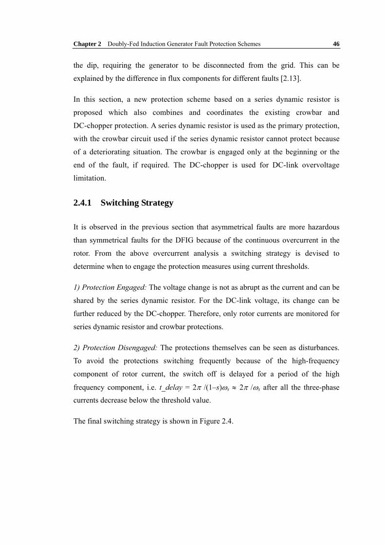
Chapter 2 Doubly-Fed Induction Generator Fault Protection Schemes 46
the dip, requiring the generator to be disconnected from the grid. This can be
explained by the difference in flux components for different faults [2.13].
In this section, a new protection scheme based on a series dynamic resistor is
proposed which also combines and coordinates the existing crowbar and
DC-chopper protection. A series dynamic resistor is used as the primary protection,
with the crowbar circuit used if the series dynamic resistor cannot protect because
of a deteriorating situation. The crowbar is engaged only at the beginning or the
end of the fault, if required. The DC-chopper is used for DC-link overvoltage
limitation.
2.4.1 Switching Strategy
It is observed in the previous section that asymmetrical faults are more hazardous
than symmetrical faults for the DFIG because of the continuous overcurrent in the
rotor. From the above overcurrent analysis a switching strategy is devised to
determine when to engage the protection measures using current thresholds.
1) Protection Engaged: The voltage change is not as abrupt as the current and can be
shared by the series dynamic resistor. For the DC-link voltage, its change can be
further reduced by the DC-chopper. Therefore, only rotor currents are monitored for
series dynamic resistor and crowbar protections.
2) Protection Disengaged: The protections themselves can be seen as disturbances.
To avoid the protections switching frequently because of the high-frequency
component of rotor current, the switch off is delayed for a period of the high
frequency component, i.e. t_delay = 2π /(1–s)ωs ≈ 2π /ωs after all the three-phase
currents decrease below the threshold value.
The final switching strategy is shown in Figure 2.4.
Chapter 2 Doubly-Fed Induction Generator Fault Protection Schemes 47
> ir, abc
Ith_SDR Series Dynamic Resistor ON
Crowbar OFF Rotor-Side Converter ON
AND
Timer t_delay = 2π/(1–s)ωs
Series Dynamic Resistor OFF
< vDC
Vth_DC DC-Chopper ON
> ir, abc
Ith_CB
AND Crowbar ON Rotor-Side Converter OFF
DC-Chopper OFF
Figure 2.4: Combined converter protection switching strategy (for subscripts: th – threshold values;
CB – Crowbar; SDR – Series Dynamic Resistor).
2.4.2 Series Dynamic Resistance Calculations
Resistance values are calculated for the most serious condition (with the highest peak
current value): symmetrical voltage dip up to 1.0 p.u. The rotor current expressions
are (2.15) − (2.19). Due to the small stator resistance, the following approximations
are made: 1/ ≈− ste τ ; τ ≈ τr.
Then, the current components are expressed as a single trigonometric function as
( )
r
t
rs
ms
rr
sr
r
rraDC es
LLV
LV
sLtii τ
ωττ
σβ
ωττ
σ
−−
⎪⎭
⎪⎬⎫
⎪⎩
⎪⎨⎧
+−−
+−= 22220 1
)1(1cos1
1)( (2.44)
)sin(1 22
ϕβωωτ
τσ
+++
= tsL
Vi s
rr
r
r
rvr
(2.45)
0=vrfi (2.46)
)sin(1
)1(122
ϕωωτ
τσ
++
−= tsLLV
Li r
rr
r
s
ms
rvrn
(2.47)
where ⎟⎟⎠
⎞⎜⎜⎝
⎛= −
rrωτϕ 1tan 1 .

Chapter 2 Doubly-Fed Induction Generator Fault Protection Schemes 48
Considering the amplitude of each component at the maximum current value
2222220max,1
)1(111
)1(1)(rr
r
s
ms
rrr
r
r
r
rr
r
s
ms
rrara s
LLV
LLVs
LLV
Ltii
ωττ
σωττ
σωττ
σ +−+
++
+−−= − . (2.48)
Also, the boundary conditions are
ira,max ≤ Ith_SDR, Vr ≤ Vth_RSC. (2.49)
Therefore, (2.48) and (2.49) are equations where τr can be solved. With the
protection schemes
protectionr
rr RR
L+
=στ . (2.50)
Then, the critical resistance value Rprotection can be calculated. If the rotor fault
currents still cannot be limited effectively, the crowbar can be used as further
protection. The total resistance is Rprotection, includes RSDR and RCB. The
current-limiting function is provided by the series dynamic resistor, hence the critical
criterion of crowbar resistance is the voltage across it must be within the rotor
voltage limit, for its shunt connection: RCB×ir,max ≤ Vr,max. Therefore, the crowbar
resistance is a small contribution to the total Rprotection. This is simpler than using
crowbar protection alone, where the resistance has a lower and upper limit. The
minimum value of resistance is restricted by the rotor winding current limit, while
the maximum is set by the voltage limit at the converter terminals [2.5].
2.5 Simulation Results
The proposed converter protection method is verified by PSCAD/EMTDC
simulations. The generator parameters are listed in Table 2.3. The faults simulated
are:
1) a three-phase voltage dip of 0.95 p.u. for 0.2 s;
2) a single-phase (phase a) grounding for 0.2 s;

Chapter 2 Doubly-Fed Induction Generator Fault Protection Schemes 49
3) a two-phase short-circuit (phase b to c) for 0.2 s; and
4) a three-phase voltage dip of 0.6 p.u. for 1.0 s.
The threshold values for calculating RSDR and RCB are set as Ith_SDR = 1.5 p.u., Ith_CB =
1.8 p.u. Rotor slip is s = –0.2 p.u. preceding the faults.
From (2.48) and (2.49), τr = 0.65 ms, Rprotection = 0.987 p.u. = 0.59 Ω. Then, the
selected resistance values are RSDR = 0.5 Ω, RCB = 0.09 Ω. The value of DC-chopper
resistance is not so critical as it is only related to the DC-link voltage, so here choose
RDCC = 0.5 Ω.
2.5.1 Symmetrical Fault Condition
Figures 2.5 and 2.6 show the system response to a 0.95 p.u. voltage dip for 0.2 s with
and without protection respectively. In the simulation without protection, the
rotor-side converter is blocked during the fault. The rotor currents reach around
10.0p.u. for the most serious phase. DC-link voltage and rotor speed both increase
until the fault is cleared. Large electrical torque fluctuations occur.
In Figure 2.6, series dynamic resistor is switched in ten times in total to limit the
rotor current. During the recovery of the fault, crowbar is switched in for five times
with the series dynamic resistor connected as the rotor current increases beyond the
crowbar threshold. The simulation results show that with series dynamic resistor
protection, the first torque peak is safely avoided, while crowbar is helpful for
protection during fault recovery. The rotor current amplitude is limited within 1.5
p.u., as required. This also restricts the DC-link voltage increase (less than 0.05 p.u.
in Figure 2.6). The DC-chopper function is not required. The rotor speed increase is
effectively restrained from 1.2 p.u. to 1.207 p.u. compared to 1.22 p.u. without
protection.
The large 5.0 p.u. torque fluctuation at the start of the fault is avoided; compare
Figure 2.5 to Figure 2.6 with the series dynamic resistor. However, a 7.0 p.u. torque
fluctuation occurs during the fault recovery phase in Figure 2.6. This is due to the
crowbar protection switching in as a further protection measure. The individual
crowbar and SDR torque performances will be compared in Section 2.5.3 which

Chapter 2 Doubly-Fed Induction Generator Fault Protection Schemes 50
shows that all of the 7.0 p.u. torque pulsation that occurs at fault recovery is due to
the crowbar circuit [see Figure 2.10 (d) and (e)]. Note that in Figure 2.5, Tm is in blue
and Te is in green and that in Figure 2.6, Tm is in green while Te is in blue.
Figure 2.5: Three-phase 0.95 p.u. voltage dip for 0.2 s without protection: (a) three-phase stator
voltages vs a,b,c [in per unit (p.u.)]; (b) three-phase stator currents is a,b,c (p.u.); (c) three-phase rotor
currents ir a,b,c (p.u.); (d) phase-a rotor voltage vra (p.u.) and phase-a RSC voltage vrsc,a (p.u.); (e)
DC-link voltage vDC (p.u.); (f) stator side active power Ps (p.u.) and reactive power Qs (p.u.); (g) rotor
speed ωr (p.u.); (h) electrical torque Te (p.u.) and mechanical torque Tm (p.u.).
(a)
(b)
(c)
(d)
(e)
(f)
(g)
(h)

Chapter 2 Doubly-Fed Induction Generator Fault Protection Schemes 51
Figure 2.6: Three-phase 0.95 p.u. voltage dip for 0.2 s with converter protection: (a) three-phase stator voltages vs a,b,c [in per unit (p.u.)]; (b) three-phase stator currents is a,b,c (p.u.); (c) three-phase rotor currents ir a,b,c (p.u.); (d) SDR switching signal SSDR; (e) crowbar switching signal SCB; (f) DC-chopper switching signal SDCC; (g) phase-a rotor voltage vra (p.u.) and phase-a RSC voltage vRSC,a (p.u.); (h) DC-link voltage vDC (p.u.); (i) stator side active power Ps (p.u.) and reactive power Qs (p.u.); (j) rotor speed ωr (p.u.); (k) electrical torque Te (p.u.) and mechanical torque Tm (p.u.).
(a)
(b)
(c)
(d)
(e)
(f)
(g)
(h)
(i)
(j)
(k)

Chapter 2 Doubly-Fed Induction Generator Fault Protection Schemes 52
Although there is no rotor voltage monitoring in the switching strategy, it is still
limited effectively to the value before the fault because of the voltage sharing ability
of the series dynamic resistor. The rotor voltages display switching frequency
components due to the pulse-width modulation of the rotor-side converter. The high
voltage is shared across the series resistor and the converter which results in a lower
converter side voltage (vRSC,a in Figure 2.7).
Large transients occur during the fault clearing mainly due to the impact of crowbar
protection switching, but together with series dynamic resistor protection, the
disturbances are clamped after about 0.05 s. It should be noted that whilst the
crowbar is used in this particular case, it is not necessary under all faults.
Figure 2.7: The rotor voltage vra [in per unit (p.u.)] and rotor-side converter voltage vRSC,a (p.u.)
comparison (zoomed from 1 s to 1.1 s).
2.5.2 Asymmetrical Fault Conditions
Figures 2.8 and 2.9 show the system responses during asymmetrical fault conditions.
The rotor currents are also limited within 1.5 p.u. For the phase-a fault in Figure 2.8,
the series dynamic resistor and crowbar protection switching events are similar to the
symmetrical fault conditions. However, there is one period of DC-chopper switching
because of the gradual increase of DC-link voltage to 1.1 p.u. Instead of increasing,
the rotor speed decreases because the DFIG is still under control with active power
supplied to the grid. An overspeed condition is avoided as the electrical torque
balances the mechanical torque from the wind turbine’s blade system.
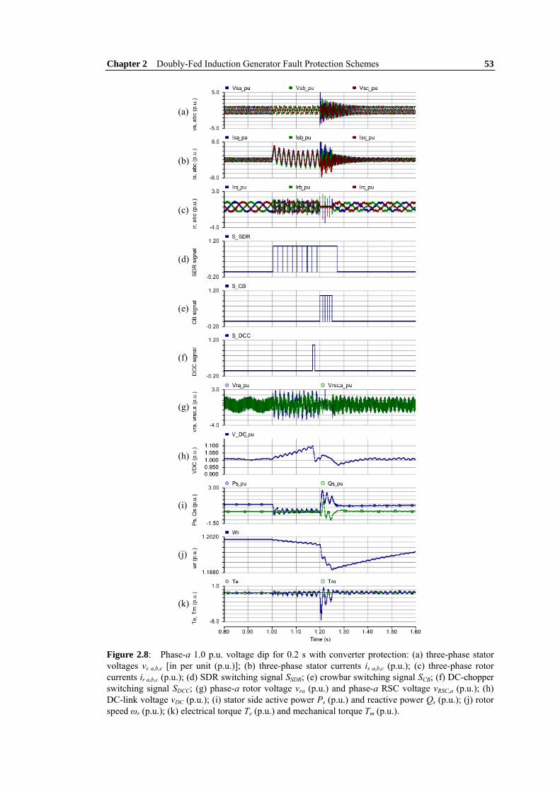
Chapter 2 Doubly-Fed Induction Generator Fault Protection Schemes 53
Figure 2.8: Phase-a 1.0 p.u. voltage dip for 0.2 s with converter protection: (a) three-phase stator voltages vs a,b,c [in per unit (p.u.)]; (b) three-phase stator currents is a,b,c (p.u.); (c) three-phase rotor currents ir a,b,c (p.u.); (d) SDR switching signal SSDR; (e) crowbar switching signal SCB; (f) DC-chopper switching signal SDCC; (g) phase-a rotor voltage vra (p.u.) and phase-a RSC voltage vRSC,a (p.u.); (h) DC-link voltage vDC (p.u.); (i) stator side active power Ps (p.u.) and reactive power Qs (p.u.); (j) rotor speed ωr (p.u.); (k) electrical torque Te (p.u.) and mechanical torque Tm (p.u.).
(a)
(b)
(c)
(d)
(e)
(f)
(g)
(h)
(i)
(j)
(k)

Chapter 2 Doubly-Fed Induction Generator Fault Protection Schemes 54
Figure 2.9: Phase b to c short circuit for 0.2 s with converter protection: (a) three-phase stator voltages vs a,b,c [in per unit (p.u.)]; (b) three-phase stator currents is a,b,c (p.u.); (c) three-phase rotor currents ir a,b,c (p.u.); (d) SDR switching signal SSDR; (e) crowbar switching signal SCB; (f) DC-chopper switching signal SDCC; (g) phase-a rotor voltage vra (p.u.) and phase-a RSC voltage vRSC,a (p.u.); (h) DC-link voltage vDC (p.u.); (i) stator side active power Ps (p.u.) and reactive power Qs (p.u.); (j) rotor speed ωr (p.u.); (k) electrical torque Te (p.u.) and mechanical torque Tm (p.u.).
(a)
(b)
(c)
(d)
(e)
(f)
(g)
(h)
(i)
(j)
(k)

Chapter 2 Doubly-Fed Induction Generator Fault Protection Schemes 55
The phase b to c short-circuit in Figure 2.9, in terms of fault current, is less serious
than in the single-phase case. There is no need for both crowbar and DC-chopper
operation. The series dynamic resistor is effective in this condition. But in terms of
stator voltage, this is more serious than for a single-phase fault. There are much
larger power and electrical torque fluctuations during the fault. This results in
gradual increase of rotor speed, from 1.20 p.u. to 1.21 p.u. but this is not serious.
The two asymmetrical conditions result in fluctuations after stator voltage recovery.
Although most of the variables are under control, these fluctuations should be studied
in more detail.
2.5.3 Performance Comparison Between Crowbar and SDR
The performance of the crowbar and the series dynamic resistor protection schemes
are compared. The reactive power, electrical torque and rotor speed of the DFIG
system are simulated and compared in Figure 2.10.
Both of the two strategies experience reactive power and electrical torque
fluctuations during the fault. However, for crowbar protection, they are much larger.
Figure 2.10(b) is expanded to show the reactive power. It can be seen that with the
rotor-side converter connected with the series dynamic resistor protection scheme, no
reactive power is absorbed. However, for crowbar protection, the asynchronous
machine absorbs reactive power, up to 0.2 p.u. Therefore, in terms of grid voltage
recovery, the series dynamic resistor protection has a significant advantage, as it
doest not further contribute to voltage drop in the network due to reactive power.
The reactive power and electrical torque ripples are larger with series dynamic resistor
protection compared to crowbar protection. This is due to the higher resistance in the
rotor winding and DFIG control system performance during faults, which needs further
exploration. However, it is clear that the peak torque that occurs at crowbar turn-on and
turn-off is significantly higher than that for the series dynamic resistor. This leads to the
large torque fluctuation seen in Figure 2.6 when the crowbar is engaged. For rotor speed
changes they are about 0.02 p.u. different at the peak prior to recovery. The series
dynamic resistor reduces the rotor overspeed more effectively than the crowbar circuit.

Chapter 2 Doubly-Fed Induction Generator Fault Protection Schemes 56
0.5 1 1.5 2 2.5
-0.6
-0.4
-0.2
0
0.2
0.4
0.6
Qs
(p.u
.)
SDRCB
(a)
1 1.1 1.2 1.3 1.4 1.5 1.6 1.7 1.8 1.9 2-0.2
-0.1
0
0.1
0.2
Qs
(p.u
.)
SDRCB
(b)
0.5 1 1.5 2 2.5
1.2
1.22
1.24
1.26
1.28
1.3
Wr (
p.u.
)
CBSDR
(c)
0.5 1 1.5 2 2.5-4
-3
-2
-1
0
1
Te (p
.u.)
CB
0.5 1 1.5 2 2.5-1.5
-1
-0.5
0
0.5
1
Te (p
.u.)
SD
R
time (s)
(d)
(e)
Figure 2.10: System response comparison between crowbar and series dynamic resistor protections, voltage dip of 0.6 p.u. for 2 s: (a) stator-side reactive power Qs [in per unit (p.u.)]; (b) zoomed reactive power Qs (p.u.); (c) rotor speed ωr (p.u.); (d) electrical torque Te (p.u.) with CB protection; (e) electrical torque Te (p.u.) with SDR protection.
More importantly, the series dynamic resistor has a much smaller impact than the
crowbar, especially during switching off. Improper crowbar switch-off strategy
(without the coordination of controller reference setting [2.1]) can cause frequent
switching which affects fault recovery. This can also be seen from the comparison of
voltage recovery in Figures 2.8 and 2.9. Without crowbar switching, the voltage
recovery for the two-phase short-circuit shows minimal fluctuation.

Chapter 2 Doubly-Fed Induction Generator Fault Protection Schemes 57
2.6 Application Discussions
2.6.1 Switch Time of the Bypass Switch
In practical applications, the switch time may be an issue, especially for serious fault
protection and recovery when fast switching response is required, e.g., some crowbar
thyristor switches cannot interrupt the current before zero-crossing [2.2]. This will
influence the protection performance. In the above simulations, switching times of
the crowbar and series-dynamic-resistor power electronic switches are considered by
disabling the interpolation in PSCAD/EMTDC. This solves the conflict between
immediate switching operation with simulation time step. The simulation time step is
set as 20 μs, so the actual switch time for IGBT is 20 μs, which is enough for the
IGBTs in applications (commonly several microseconds [2.14]).
2.6.2 Switch Normal Operation Losses
The series dynamic resistor is here realised by a power electronic switch. However,
the bypass switch that is closed during normal operation will produce additional
losses, specifically device ON-state losses. But compared to the stator side braking
resistor bypass-switches [2.10], this is far lower due to the lower power rating on the
rotor side.
2.7 Conclusion
Converter protection is necessary for DFIG wind power generation systems during
fault conditions. In this chapter, various resistor protection schemes are reviewed.
The purposes of a series dynamic resistor are: 1) to avoid the frequent use of crowbar
short-circuit, 2) to maximise the operation time of the rotor-side converter, and 3) to
reduce torque fluctuations during protection operation. The rotor currents during
various fault conditions are discussed and current expressions are given to instruct
the design of the protection scheme. Resistance calculations for the series dynamic
resistor and crowbar using the expression of maximum rotor current are described.

Chapter 2 Doubly-Fed Induction Generator Fault Protection Schemes 58
The series dynamic resistor can operate with the rotor-side converter control
functioning. For the control of the grid-side converter to DC-link bus voltage, the
resumption time can be shorter than for a system with normal active crowbar
protection. This is helpful for resuming normal control and provides reactive power
for grid voltage support. During this process, inspection of the reactive power,
electrical torque, and rotor speed fluctuations shows that the proposed method
enhances DFIG fault ride-through capability. In the next chapter, the protection for
another popular wind power generation system based on PMSG is investigated.
Chapter 2 Doubly-Fed Induction Generator Fault Protection Schemes 59
2.8 References
[2.1] J. Morren, and S.W.H. de Haan, “Ridethrough of wind turbines with doubly-fed induction generator during a voltage dip,” IEEE Trans. Energy Convers., vol. 20, no. 2, pp. 435-441, Jun. 2005.
[2.2] I. Erlich, J. Kretschmann, J. Fortmann, S. Mueller-Engelhardt, and H. Wrede, “Modeling of wind turbines based on doubly-fed induction generators for power system stability studies,” IEEE Trans. Power Syst., vol. 22, no. 3, pp. 909-919, Aug. 2007.
[2.3] D. Xiang, R. Li, P. J. Tavner, and S. Yang, “Control of a doubly fed induction generator in a wind turbine during grid fault ride-through,” IEEE Trans. Energy Convers., vol. 21, no. 3, pp. 652-662, Sep. 2006.
[2.4] P. S. Flannery and G. Venkataramanan, “A fault tolerant doubly fed induction generator wind turbine using a parallel grid side rectifier and series grid side converter,” IEEE Trans. Power Electron., vol. 23, no. 3, pp. 1126-1135, May 2008.
[2.5] J. Morren and S. W. H. de Haan, “Short-circuit current of wind turbines with doubly fed induction generator,” IEEE Trans. Energy Convers., vol. 22, no. 1, pp. 174-180, Mar. 2007.
[2.6] P. Zhou and Y. He, “Control strategy of an active crowbar for DFIG based wind turbine under grid voltage dips,” in Proc. Int. Conf. Electrical Machines and System. 2007, Seoul, Korea, Oct. 8-11, 2007.
[2.7] M. Rodríguez, G. Abad, I. Sarasola, and A. Gilabert, “Crowbar control algorithms for doubly fed induction generator during voltage dips,” in Proc. 11th Eur. Conf. Power Electron. Appl., Dresden, Germany, Sep. 11-14, 2005.
[2.8] I. Erlich, H. Wrede, and C. Feltes, “Dynamic behavior of DFIG-based wind turbines during grid faults,” in Proc. Power Convers. Conf., Nagoya, Japan, Apr. 2-5, 2007.
[2.9] J. F. Conroy and R. Watson, “Low-voltage ride-through of a full converter wind turbine with permanent magnet generator,” IET Renew. Power Gener., vol. 1, no. 3, pp. 182-189, 2007.
[2.10] A. Causebrook, D. J. Atkinson, and A. G. Jack, “Fault ride-through of large wind farms using series dynamic braking resistors (March 2007),” IEEE Trans. Power Syst., vol. 22, no. 3, pp. 966-975, Aug. 2007.
[2.11] J. López, P. Sanchis, X. Roboam, and L. Marroyo, “Dynamic behavior of the doubly fed induction generator during three-phase voltage dips,” IEEE Trans. Energy Convers., vol. 22, no. 3, pp. 709-717, Sep. 2007.
[2.12] M. S. Vicatos and J. A. Tegopoulos, “Transient state analysis of a doubly-fed

Chapter 2 Doubly-Fed Induction Generator Fault Protection Schemes 60
induction generator under three phase short circuit,” IEEE Trans. Energy Convers., vol. 6, no. 1, pp. 62-68, Mar. 1991.
[2.13] J. López, E. Gubía, P. Sanchis, X. Roboam, and L. Marroyo, “Wind turbines based on doubly fed induction generator under asymmetrical voltage dips,” IEEE Trans. Energy Convers., vol. 23, no. 1, pp. 321-330, Mar. 2008.
[2.14] S. Castagno, R. D. Curry, and E. Loree, “Analysis and comparison of a fast turn-on series IGBT stack and high-voltage-rated commercial IGBTs,” IEEE Trans. Plasma Science, vol. 34, no. 5, pp 1692-1696, Oct. 2006.
61
Chapter 3 Permanent Magnet Synchronous Generator Fault Protection Schemes
3.1 Introduction
Although the doubly-fed induction generator (DFIG) is a popular wind turbine
generation system due to the balance between cost and performance, as discussed in
Chapter 2, a significant disadvantage of DFIG is its vulnerability to grid disturbances
and fluctuations. This is especially true of its mechanically vulnerable gearbox.
According to statistics of wind farm operation, 19.4% of wind turbine downtime is
due to the gearbox and bearing system [3.1]. Recently, the development of
larger-scale wind power generation systems has considered topologies with
direct-driven permanent magnet synchronous generators (PMSGs), which do not use
a gearbox, hence may be more reliable.
PMSG energy conversion systems can be classified into two categories: 1) connected
to two back-to-back voltage-source converters (VSCs); 2) connected to a diode
rectifier with DC/DC boost converter and a voltage-source inverter (VSI). The
former is commonly considered as the technically ultimate option but is more
expensive and complex. The latter is usually used in stand-alone or small-scale wind
farms or micro-grids because of its simple topology and control, and most
importantly, low cost. In this chapter, both topologies are considered.
Currently, PMSG system studies consider normal operation and the realisation of
variable-speed maximum power point tracking. Research into system protection is
limited at this stage [3.2], [3.3]. However, as fault ride-through (FRT) requirements
have been proposed and there are increasing requirements for operation under harsh
offshore environments, protection schemes are gradually being proposed and applied

Chapter 3 Permanent Magnet Synchronous Generator Fault Protection Schemes 62
for many wind power generation systems. The protection of wind farm devices,
particularly the power electronic devices, is initially more important than staying
connected to the grid.
Hence this chapter analyses the protection issues of PMSG systems and is organised
as follows. In Section 3.2, the two PMSG power conversion systems and their
control strategies are described. Section 3.3 introduces the options of protection
schemes. PSCAD/EMTDC simulation results are provided in Section 3.4 to verify
the proposed protection schemes.
The DC wind farm considered in this chapter assumes parallel-connected wind
turbine generator systems. After collection from the generation systems, DC power is
transmitted to the grid through DC transmission cables, a vector-controlled
voltage-source inverter and a step-up transformer. The wind farm collection and
transmission network protection issues will be analysed in Chapters 4 and 5.
Different wind turbine converter topologies have different fault characteristics; hence
only typical fault conditions are analysed for each topology.
3.2 Direct-Driven PMSG Wind Power Generation Systems
3.2.1 PMSG Power Conversion Topologies
The PMSG is used for direct-driven applications because of its simple winding
structure, ease of control, and the ease of which multi-pole machines can be realised.
The studied systems are: a three-phase diode rectifier with a DC/DC boost converter,
and; a six-IGBT/diode bridge voltage-source converter. The basic topologies are
shown in Chapter 1, Figures 1.3 and 1.4.
These generation systems have multi-pole PMSGs and fully rated power converters
connecting the system to the grid. As mentioned, a direct-driven multi-pole PMSG is
more reliable as it eliminates the gearbox. The fully rated power converter gives
potentially improved technical performance but produces more losses in the power
conversion process. Three-phase diode-rectifier and a DC/DC boost converter
configuration is mainly based on low cost and simple topology [3.2], [3.3]. The diode

Chapter 3 Permanent Magnet Synchronous Generator Fault Protection Schemes 63
rectifier converts generator AC power into DC in an uncontrolled manner; therefore,
power control has to be performed by the VSC connected to the grid. When the
generator speed varies, the DC voltage after the diode rectifier will change. A boost
converter is used to provide a smooth DC-link voltage to the inverter. The control of
generator torque and speed is realised by controlling the inductor current in the boost
converter. It is cheaper and the generator is decoupled from the grid by the DC-link
which supplies the pulse-width modulated inverter. The aim of the grid-side VSI is to
provide connection to the onshore grid with a steady DC-link voltage and adjustment
of the coupling point power factor or reactive power using standard techniques.
The two topologies can be seen as a current source (boost) and a voltage source,
respectively. Hence the current source converter is vulnerable to open-circuit faults
and the voltage source converter is vulnerable to short-circuit faults. The system
protection will be designed to cope with these most serious conditions.
The generator equations under DC short-circuit fault conditions are in terms of the
stator currents in dq reference frame and per unit value. State variables are stator
currents isd, isq and rotor speed ωr.
0)()()( =+−+++ sqrssd
ssds iLLdt
diLLiRR ω (3.1)
0)()()( =Ψ−+++++ rsdrssq
ssqs iLLdt
diLLiRR ωω (3.2)
)5.1(1rmrsq
r PFipJdt
d ωωω−−Ψ= (3.3)
3),( windpm vCP βλ= (3.4)
where Rs, Ls, R, and L are the generator stator winding resistance and inductance,
fault point equivalent resistance and inductance, respectively. J = 2.0 p.u. is the shaft
rotating inertia. p is the pole pair. Ψ = 1.0 p.u. is the constant magnet flux. F = 0.002
is the shaft friction damping factor. Wind turbine power Pm is calculated from
equation (3.4). Detailed equations are referred to Chapter 1 – equation (1.3). Base
values are the ratings of the generators; base wind speed is 12 ms–1.

Chapter 3 Permanent Magnet Synchronous Generator Fault Protection Schemes 64
It is difficult to get an analytical solution with the complex wind turbine power
expression (3.4). Hence in the following section, numerical simulation is used to
demonstrate the protection schemes and their performances.
3.2.2 Control Strategy
The focus of this research is the protection scheme design and analysis. Hence a
common control strategy is applied. For a large-scale system, a voltage-source
converter is used for maximum power point tracking. The large-scale wind turbine
has pitch-control function to reduce turbine shaft overspeed. For a small-scale system,
the boost IGBT switching signal is a duty ratio, which is obtained from a PI
controller that eliminates the difference between the rectified DC power and
reference turbine power [3.4]. The grid-side voltage-source inverter is
vector-controlled. In the synchronous speed rotating reference frame under grid
voltage vector, the angle of dq transformation θe is used for decoupling control [3.5].
All the inverters in the PSCAD/EMTDC simulation use sinusoidal PWM vector
control.
3.3 PMSG System Protection
The study of the HVDC transmitted wind farm protection during the grid fault has
been reported [3.6]. The main protection is connecting a DC-link damping resistor to
limit the DC-link overvoltage through energy dissipation. This is also analysed for a
PMSG stand-alone system for protection [3.7].
Because there is no induced rotor overcurrent to limit during fault conditions, the
major issue is to protect the system through DC-link energy transmission. The
DC-link damping resistor method can be used in this case. One particular solution for
this method in PMSG system is using one more DC/DC boost converter [3.8]. The
detailed protection circuit topologies for DC-links are shown in [3.9]-[3.11]. There
are mainly two types, either with a resistor to dissipate the redundant energy or
incorporating an energy storage system (ESS).
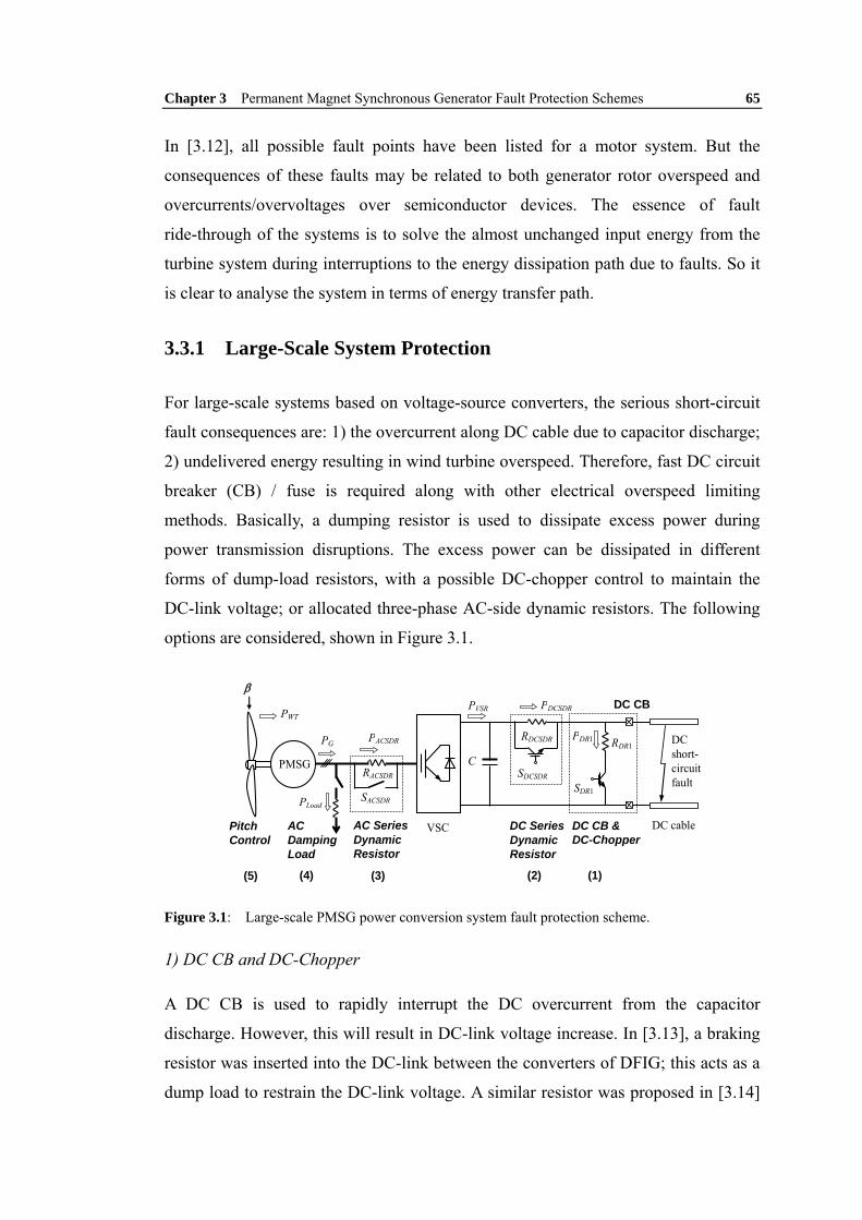
Chapter 3 Permanent Magnet Synchronous Generator Fault Protection Schemes 65
In [3.12], all possible fault points have been listed for a motor system. But the
consequences of these faults may be related to both generator rotor overspeed and
overcurrents/overvoltages over semiconductor devices. The essence of fault
ride-through of the systems is to solve the almost unchanged input energy from the
turbine system during interruptions to the energy dissipation path due to faults. So it
is clear to analyse the system in terms of energy transfer path.
3.3.1 Large-Scale System Protection
For large-scale systems based on voltage-source converters, the serious short-circuit
fault consequences are: 1) the overcurrent along DC cable due to capacitor discharge;
2) undelivered energy resulting in wind turbine overspeed. Therefore, fast DC circuit
breaker (CB) / fuse is required along with other electrical overspeed limiting
methods. Basically, a dumping resistor is used to dissipate excess power during
power transmission disruptions. The excess power can be dissipated in different
forms of dump-load resistors, with a possible DC-chopper control to maintain the
DC-link voltage; or allocated three-phase AC-side dynamic resistors. The following
options are considered, shown in Figure 3.1.
PMSG C
DC cable VSC
RDCSDR
SDCSDR
RDR1
SDR1
PDR1
DC SeriesDynamic Resistor
DC CB & DC-Chopper
AC Damping Load
PWT
PG
PDCSDRPVSR
PLoad
DC CB
DC short- circuit fault
RACSDR
PACSDR
SACSDR
AC SeriesDynamic Resistor
Pitch Control
β
(1)(2)(3)(4) (5)
Figure 3.1: Large-scale PMSG power conversion system fault protection scheme.
1) DC CB and DC-Chopper
A DC CB is used to rapidly interrupt the DC overcurrent from the capacitor
discharge. However, this will result in DC-link voltage increase. In [3.13], a braking
resistor was inserted into the DC-link between the converters of DFIG; this acts as a
dump load to restrain the DC-link voltage. A similar resistor was proposed in [3.14]
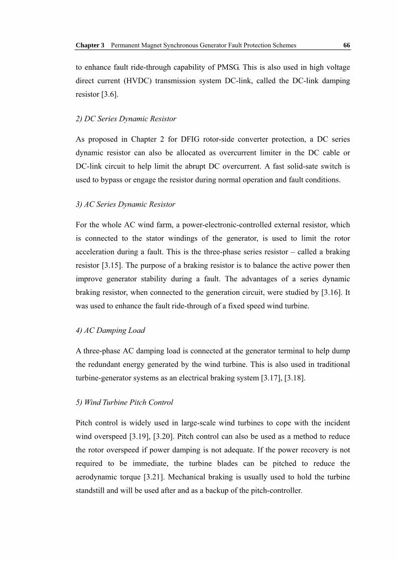
Chapter 3 Permanent Magnet Synchronous Generator Fault Protection Schemes 66
to enhance fault ride-through capability of PMSG. This is also used in high voltage
direct current (HVDC) transmission system DC-link, called the DC-link damping
resistor [3.6].
2) DC Series Dynamic Resistor
As proposed in Chapter 2 for DFIG rotor-side converter protection, a DC series
dynamic resistor can also be allocated as overcurrent limiter in the DC cable or
DC-link circuit to help limit the abrupt DC overcurrent. A fast solid-sate switch is
used to bypass or engage the resistor during normal operation and fault conditions.
3) AC Series Dynamic Resistor
For the whole AC wind farm, a power-electronic-controlled external resistor, which
is connected to the stator windings of the generator, is used to limit the rotor
acceleration during a fault. This is the three-phase series resistor – called a braking
resistor [3.15]. The purpose of a braking resistor is to balance the active power then
improve generator stability during a fault. The advantages of a series dynamic
braking resistor, when connected to the generation circuit, were studied by [3.16]. It
was used to enhance the fault ride-through of a fixed speed wind turbine.
4) AC Damping Load
A three-phase AC damping load is connected at the generator terminal to help dump
the redundant energy generated by the wind turbine. This is also used in traditional
turbine-generator systems as an electrical braking system [3.17], [3.18].
5) Wind Turbine Pitch Control
Pitch control is widely used in large-scale wind turbines to cope with the incident
wind overspeed [3.19], [3.20]. Pitch control can also be used as a method to reduce
the rotor overspeed if power damping is not adequate. If the power recovery is not
required to be immediate, the turbine blades can be pitched to reduce the
aerodynamic torque [3.21]. Mechanical braking is usually used to hold the turbine
standstill and will be used after and as a backup of the pitch-controller.

Chapter 3 Permanent Magnet Synchronous Generator Fault Protection Schemes 67
The resistance calculation is based on analysis of the redundant energy dissipation.
The energy from the wind turbine should be dissipated by the protection scheme.
Taking all the normal parameters as 1.0 per unit value, the resistance value should
also be 1.0 p.u. in the steady-state operation of the protection circuit. For example, if
the rating power of the generator is 5 MW, with a rectifier voltage of 1 kV, the
resistance value is 0.8 Ω.
3.3.2 Small-Scale System Protection
For small-scale systems, there is usually no pitch control system in each wind
turbine’s blade. Therefore it is not included in the protection scheme below. The AC
series dynamic resistor is also not included as from the above large-scale system
analysis, it is similar to DC ones.
Diode Rectifier
DC/DC Boost Converter
RDR1
SDR1
PDR1
DC-link Damping Resistor1
PRec
L
S
RSDR
SSDR
Series Dynamic Resistor
DC cable
DC open circuit fault
PMSG
Damping Load
PWT
PG
PLoad
PSDR DC CB
Figure 3.2: Small-scale PMSG power conversion system fault protection scheme.
1) Redundant Energy Dissipation or Storage
As in the Section 3.3.1, protection devices can be used at different links of the
system [3.7], [3.9]-[3.11], [3.20]. Each DC-link connection point in the generation
system can be seen as an energy balance point to analyse appropriate protection
schemes. The protection options for small-scale systems are shown in Figure 3.2.
The dotted blocks are the positions of the main protection schemes which can also be
replaced by other specific circuit, e.g. energy storage devices.
Figure 3.3 shows the systems with VSI DC-link protection. The excess energy can be
dissipated through the two DC-link damping resistors, with power of PDR1 and PDR2,
depending on the fault location. The switching signals for the two switches SDR1 and
SDR2 depend on the detection of DC-link overvoltages in correspondence with a

Chapter 3 Permanent Magnet Synchronous Generator Fault Protection Schemes 68
preset threshold value. The series connected dynamic resistor RSDR can be used for
inductor overcurrent and sharing overvoltage for the IGBT switch S.
VSI Diode Rectifier
DC/DC Boost Converter
RDR1
SDR1
PDR1 RDR2
SDR2
PDR2
DC-link Damping Resistor1
DC-link Damping Resistor2
PRec
L
PInv
S
RSDR
SSDR
Series Dynamic Resistor
Figure 3.3: PMSG converter protection schemes.
2) Converter Protection Scheme for Open-Circuit Fault
The DC-link damping resistor across the grid-side VSI mainly copes with grid fault
conditions, in which the energy cannot be transmitted through the inverter so causing
DC-link overvoltage. Also, the other two resistors located in the generation system
are mainly dealing with the wind farm inner fault generally resulting in the loss of
connection to the collection grid and DC cables. The energy flows are discussed as
follows for the two protection schemes respectively.
After disconnection from the collection grid, the energy that needs to be dissipated
are from the rectifier PRec and that already stored in the inductor PL. For the power
PRec, the protection is also important to restrain the rotor overspeed. The abrupt
change of real power from the generator is in relation to the generator electrical
torque output. While the relatively slow mechanical dynamics of the rotor mean the
mechanical torque cannot be balanced with the reduced electrical torque which
results in rotor overspeed. The power PL is mainly related to the overcurrent of the
IGBT switch S.
If the DC-link Damping Resistor1 is engaged, there will be two power flow paths as
shown in Figure 3.4. Therefore, a bi-directional switch SDR1 is required. Although
theoretically this protection will work at the same way with a connection across the
inverter DC-link capacitor, the major difference is that a small capacitor Cf is only
for remedying rectifier voltage ripple instead of energy storage as is the case with
capacitor C.
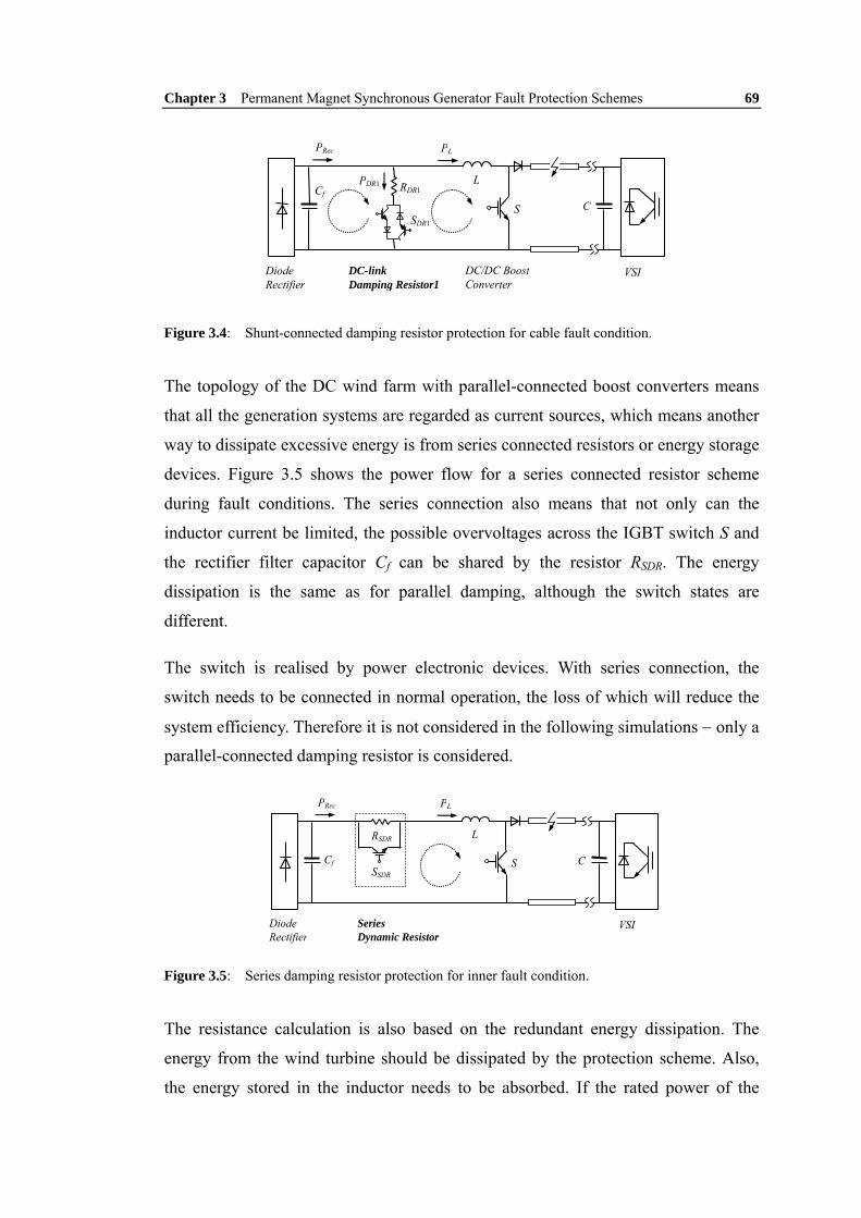
Chapter 3 Permanent Magnet Synchronous Generator Fault Protection Schemes 69
VSI Diode Rectifier
DC/DC Boost Converter
RDR1
SDR1
PDR1
DC-link Damping Resistor1
PRec
L
PL
S Cf
C
Figure 3.4: Shunt-connected damping resistor protection for cable fault condition.
The topology of the DC wind farm with parallel-connected boost converters means
that all the generation systems are regarded as current sources, which means another
way to dissipate excessive energy is from series connected resistors or energy storage
devices. Figure 3.5 shows the power flow for a series connected resistor scheme
during fault conditions. The series connection also means that not only can the
inductor current be limited, the possible overvoltages across the IGBT switch S and
the rectifier filter capacitor Cf can be shared by the resistor RSDR. The energy
dissipation is the same as for parallel damping, although the switch states are
different.
The switch is realised by power electronic devices. With series connection, the
switch needs to be connected in normal operation, the loss of which will reduce the
system efficiency. Therefore it is not considered in the following simulations − only a
parallel-connected damping resistor is considered.
VSI Diode Rectifier
PRec PL
S
RSDR
SSDR
Series Dynamic Resistor
L
C Cf
Figure 3.5: Series damping resistor protection for inner fault condition.
The resistance calculation is also based on the redundant energy dissipation. The
energy from the wind turbine should be dissipated by the protection scheme. Also,
the energy stored in the inductor needs to be absorbed. If the rated power of the

Chapter 3 Permanent Magnet Synchronous Generator Fault Protection Schemes 70
generator is 25 kW, with rectifier voltage of 800V, the resistance value is 25.6 Ω.
There is no maximum limit for the resistance value, but a too large resistor means a
big switching impact to the system when resuming normal operation after the fault
clearance.
From the overcurrent analysis a switch-timing strategy is devised. For the activation
of the protection resistor, there are two states:
1) Boost Switch ON State: At this stage, the inductor is being charged by the rectifier.
The energy from the rectifier and that already stored in the inductor can be dissipated
via the resistor and boost switch.
2) Boost Switch OFF State: The energy from the rectifier and the inductor cannot be
released from the diode to the inverter. So it is mainly the power from rectifier being
absorbed by the damping resistor.
Hysteresis control is used to control the rectifier voltage within a preset hysteresis
band. In the following simulation, the band is set at 0.1 p.u, as will be shown in
Figure 3.10(d). The inverter DC-link damping resistor switching is also included.
3.4 Simulation Results
The proposed protection method of the specific DC wind farm system are analysed
by PSCAD/EMTDC simulations. The simulation DC wind farm system includes two
equivalent parallel-connected wind turbine generation systems. The generator and
cable parameters are listed in Tables 3.1 and 3.2, respectively.
Table 3.1: PMSG Parameters
Parameter Value Parameter Value
Rated power Pn 25 kW (small-scale) Rated power Pn 5 MW (large-scale)
Rated stator voltage Vsn 450 V (small-scale) Phase resistance 0.068 p.u. (both large- and small-scale)
Rated stator voltage Vsn 800 V (large-scale) Phase inductance 0.427 p.u. (both large- and small-scale)

Chapter 3 Permanent Magnet Synchronous Generator Fault Protection Schemes 71
Table 3.2: Large-Scale System Cable Parameters
Parameter Value Parameter Value
Resistance r 0.06 Ω/km Cable length 100 m
Inductance l 0.28 mH/km DC-link capacitor 10 mF
Rating voltage 2 kV
3.4.1 Large-Scale System Fault Condition
Figure 3.6 shows the system response to a cable short-circuit fault without and with
different electrical braking system protections. The fault simulated is a permanent
fault. Without any protection, the cable overcurrent reaches 10 times of the normal
value, in Figure 3.6(a). The DC-link voltage falls to around zero rapidly. Generator
stator current increases up to 2.0 p.u. Moreover, the rotor speed ramps up to over 1.5
p.u. within 3 s, which is a heavy burden for the mechanical system.
With a fast DC CB to interrupt overcurrent above 1.5 p.u. [in Figure 3.6(b)], the
generator energy will store in the DC-link capacitor and hence there is an increase in
the DC-link voltage. However, this is not over the 1.1 p.u. limit (2.2 kV) in Figure
3.6(b) until 2.7 s. Then the hystersis control of DC-chopper starts damping energy
via the parallel-connected resistor. The rotor overspeed then begins to decrease.
Without the DC CB, only using DC series dynamic resistor to limit the stator
overcurrent and damping the redundant energy, the rotor overspeed is reduced better
in Figure 3.6(c). The AC series dynamic resistor has a similar effect in reducing the
overspeed. However, the AC switch is slow (in terms of 10 ms). This will not avoid
the first overcurrent wave front of stator current in Figure 3.6(d). A damping load in
line with AC CB (also operates in 10 ms) will almost eliminate the overspeed caused
by power unbalance, but it has no effect on the overcurrent, as shown in Figure
3.6(e).

Chapter 3 Permanent Magnet Synchronous Generator Fault Protection Schemes 72
(a) (b)
(c) (d)
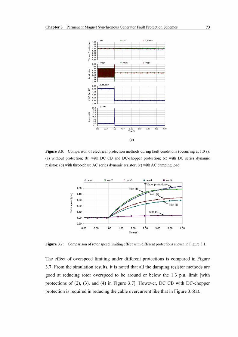
Chapter 3 Permanent Magnet Synchronous Generator Fault Protection Schemes 73
(e)
Figure 3.6: Comparison of electrical protection methods during fault conditions (occurring at 1.0 s):
(a) without protection; (b) with DC CB and DC-chopper protection; (c) with DC series dynamic
resistor; (d) with three-phase AC series dynamic resistor; (e) with AC damping load.
With (1) Without protection
With (2)
With (4)
With (3)
Figure 3.7: Comparison of rotor speed limiting effect with different protections shown in Figure 3.1.
The effect of overspeed limiting under different protections is compared in Figure
3.7. From the simulation results, it is noted that all the damping resistor methods are
good at reducing rotor overspeed to be around or below the 1.3 p.u. limit [with
protections of (2), (3), and (4) in Figure 3.7]. However, DC CB with DC-chopper
protection is required in reducing the cable overcurrent like that in Figure 3.6(a).
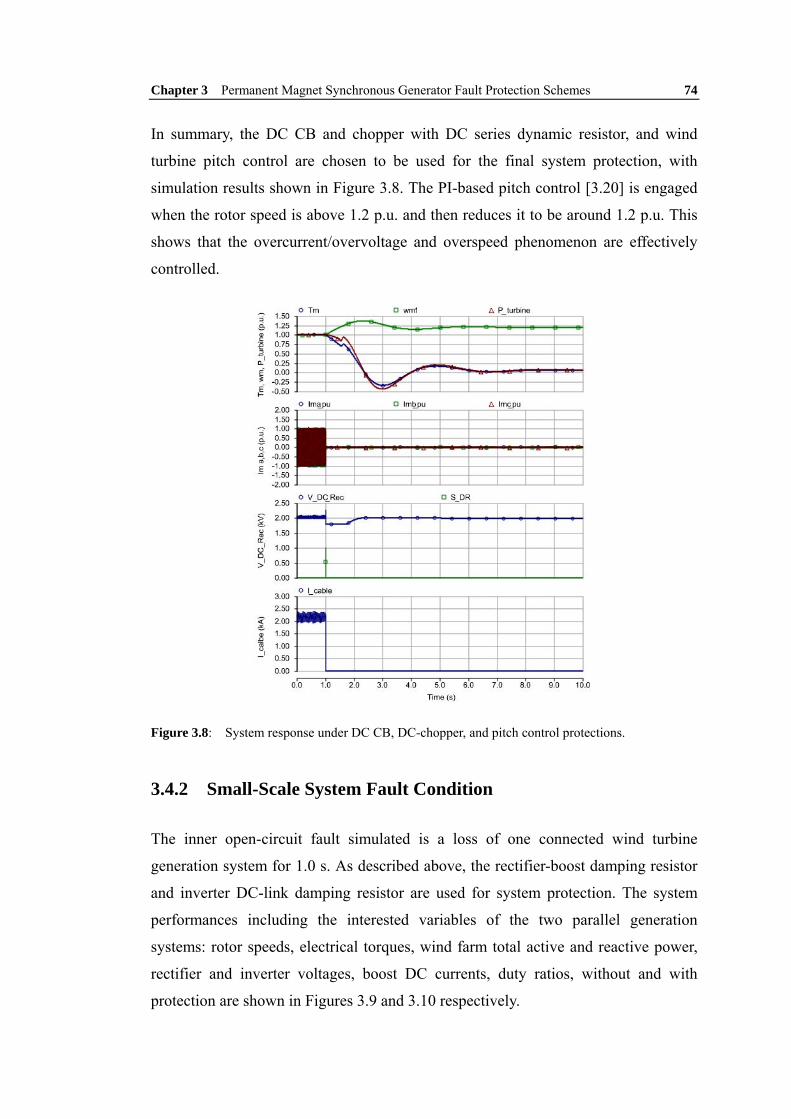
Chapter 3 Permanent Magnet Synchronous Generator Fault Protection Schemes 74
In summary, the DC CB and chopper with DC series dynamic resistor, and wind
turbine pitch control are chosen to be used for the final system protection, with
simulation results shown in Figure 3.8. The PI-based pitch control [3.20] is engaged
when the rotor speed is above 1.2 p.u. and then reduces it to be around 1.2 p.u. This
shows that the overcurrent/overvoltage and overspeed phenomenon are effectively
controlled.
Figure 3.8: System response under DC CB, DC-chopper, and pitch control protections.
3.4.2 Small-Scale System Fault Condition
The inner open-circuit fault simulated is a loss of one connected wind turbine
generation system for 1.0 s. As described above, the rectifier-boost damping resistor
and inverter DC-link damping resistor are used for system protection. The system
performances including the interested variables of the two parallel generation
systems: rotor speeds, electrical torques, wind farm total active and reactive power,
rectifier and inverter voltages, boost DC currents, duty ratios, without and with
protection are shown in Figures 3.9 and 3.10 respectively.
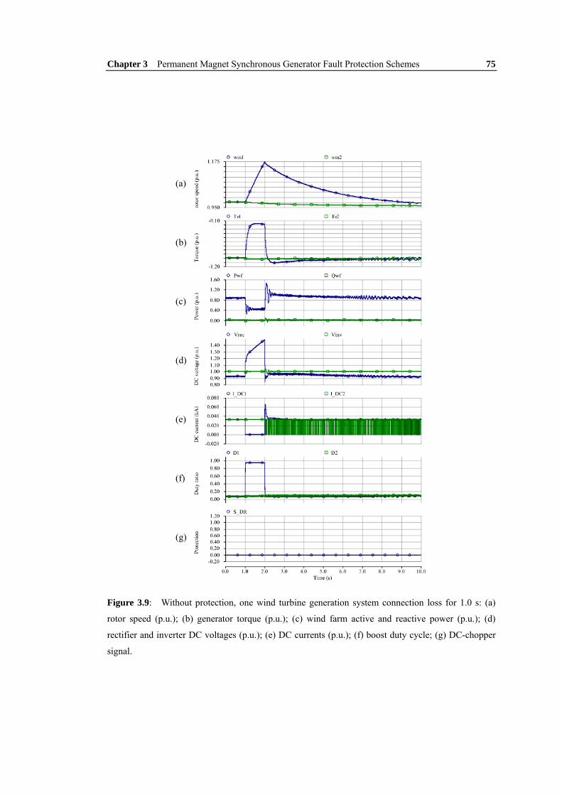
Chapter 3 Permanent Magnet Synchronous Generator Fault Protection Schemes 75
Figure 3.9: Without protection, one wind turbine generation system connection loss for 1.0 s: (a)
rotor speed (p.u.); (b) generator torque (p.u.); (c) wind farm active and reactive power (p.u.); (d)
rectifier and inverter DC voltages (p.u.); (e) DC currents (p.u.); (f) boost duty cycle; (g) DC-chopper
signal.
(a)
(b)
(c)
(d)
(e)
(f)
(g)

Chapter 3 Permanent Magnet Synchronous Generator Fault Protection Schemes 76
Figure 3.10: With protection, one wind turbine generation system connection loss for 1.0 s: (a) rotor
speed (p.u.); (b) generator torque (p.u.); (c) wind farm active and reactive power (p.u.); (d) rectifier
and inverter DC voltages (p.u.); (e) DC currents (p.u.); (f) boost duty cycle; (g) DC-chopper signal.
Without protection, the rotor speed of the first generator will accelerate rapidly as
shown in Figure 3.9(a), up to 1.175 p.u. at the end of the fault. The torque of the
faulted generator drops rapidly. Hence the total power from the wind farm decreases
to a half of its original value, with overshoot of over 1.5 p.u. at the clearance point of
the fault. Another big impact is the rectifier overvoltage, up to 1.5 p.u., during the
(a)
(b)
(c)
(d)
(e)
(f)
(g)
Chapter 3 Permanent Magnet Synchronous Generator Fault Protection Schemes 77
fault duration, which could damage the rectifier diodes. The recovery of the whole
system displays an oscillation whose amplitude rises slightly with a reducing
frequency. The influence of the fault on the inverter DC-link voltage is marginal,
within a band of 0.1 p.u. Therefore there is no need to switch in the inverter DC-link
damping resistor for protection which is why its switching signal is not shown.
With protection, the most critical values of system rotor speed and rectifier
overvoltage are effectively restrained. The active power overshoot at the fault
clearance point decreases to 1.3 p.u. The power absorbed by the damping resistor can
balance the input wind turbine power and hence limit the faulted generator rotor
speed around the value before fault, about 1.0 p.u. Rectifier voltage fluctuates within
the given hysteresis band. The whole system also experiences oscillations during the
recovery with a lower frequency than without protection. However, long term
simulations show that with protection, this oscillation is attenuated faster than the
system without protection, although with lower frequency shown in Figure 3.10
(with protection) than in Figure 3.9 (without protection).
The fluctuations are characterised by rotor speeds of the two generation systems.
When their speeds converge, the fluctuation reaches its heaviest point with biggest
amplitude. That means with protection, the process of fluctuation damping will be
faster, because the rotor speed difference is reduced by the protection scheme, from
0.175 p.u. to less than 0.05 p.u.
The oscillations during fault recovery are an interaction between the two boost-based
generation systems. Further work should be performed to understand this problem.
However it is predicted that the fluctuation is not serious, with total power
fluctuation of only about 0.05 to 0.1 p.u. If there are more paralleled-connected
systems, the situation may or may not be more complex, but may not be as a serious
influence compared to the impact of the fault on the wind farm.
The system performance and related protection schemes for other DC fault
conditions should also be analysed. The work reported in this chapter can be
combined with other protection devices such as mechanical braking devices.
However, the need to absorb excess energy cannot be avoided in this system during

Chapter 3 Permanent Magnet Synchronous Generator Fault Protection Schemes 78
fault conditions when the major problem is the interruption of the energy flow paths.
The proposed open-circuit fault protection scheme can also be used for ground faults
or short-circuit faults. With the operations of switchgear, these common faults will
result in the open-circuit status.
3.5 Conclusion
The proposed protection schemes for the direct-driven PMSG-based systems are
aimed at protecting wind farm devices and enhancing the fault ride-through
capability for grid connection. The proposed series and shunt damping resistors (AC
or DC), in the back-to-back voltage-source converter-based systems for large-scale
wind farms, and the current-source converter based systems (diode rectifier – boost
circuits) for small-scale or stand-alone wind farms are used for DC fault protection.
Both the large-scale and small-scale PMSG system protection schemes are
investigated with PSCAD/EMTDC simulations. Wind turbine blade-pitch control is
included in the large-scale system simulations for the purpose of limiting rotor
overspeed. For the small-scale parallel-connected wind farm, the normal
voltage-source inverter DC-link chopper protection is also included. The proposed
protection schemes can increase the protective flexibility and effectively protect the
system, especially for inner wind farm electrical fault conditions.
Chapter 3 Permanent Magnet Synchronous Generator Fault Protection Schemes 79
3.6 References
[3.1] J. Ribrant and L. M. Bertling, “Survey of failures in wind power systems with focus on Swedish wind power plants during 1997−2005,” IEEE Trans. on Energy Convers., vol. 22, no. 1, pp. 167-173, Mar. 2007.
[3.2] J. M. Carrasco, E. Galván, R. Portillo, L.G. Franquelo, and J.T. Bialasiewicz, “Power electronic systems for the grid integration of wind turbines,” in Proc. 32nd Annual Conf. IEEE Industrial Electronics – IECON 2006, pp. 4182-4188, Nov. 2006.
[3.3] J. A. Baroudi, V. Dinavahi, and A. M. Knight, “A review of power converter topologies for wind generators,” Renewable Energy, published online in Wiley Interscience, Jan. 19, 2007.
[3.4] S. M. Muyeen, R. Takahashi, T. Murata, and J. Tamura, “Transient stability enhancement of variable speed wind turbine driven PMSG with rectifier-boost converter-inverter,” in Proc. 18th International Conf. on Electrical Machines, 6-9 Sep. 2008.
[3.5] M. G. Molina and P. E. Mercado, “A new control strategy of variable speed wind turbine generator for three-phase grid-connected applications,” Proc. IEEE/PES Transmission and Distribution Conf. and Exposition, 13-15 Aug. 2008.
[3.6] L. Xu, L. Yao, M. Bazargan, and A. Yan, “Fault ride through of large offshore wind farms using HVDC transmission,” in Proc. IEEE Power Tech Conf., 28 Jun – 2 Jul, 2009, Bucharest, Romania.
[3.7] M. E. Haque, M. Negnevitsky, and K. M. Muttaqi, “A novel control strategy for a variable speed wind turbine with a permanent magnet synchronous generator,” Proc. Industry Applications Society Annual Meeting, 5-9 Oct. 2008.
[3.8] N. P. W. Strachan and D. Jovcic, “Dynamic modelling, simulation and analysis of an offshore variable-speed directly-driven permanent-magnet Wind Energy Conversion and Storage System (WECSS),” Europe OCEANS, June 18-21, 2007.
[3.9] C. Abbey, W. Li, L. Owatta, and G. Joós, “Power electronic converter control techniques for improved low voltage ride through performance in WTGs,” Proc. 37th IEEE Power Electronics Specialists Conference, June 18-22, 2006.
[3.10] C. Abbey and G. Joós, “Effect of low voltage ride through (LVRT) characteristic on voltage stability,” Proc. of IEEE Power Engineering Society General Meeting, Jun. 12-16, 2005, 1901-1907.
[3.11] J. Morneau, C. Abbey and G. Joós, “Effect of low voltage ride through technologies on wind farm,” IEEE Canada Electrical Power Conference, Oct. 25-26, 2007, 56-61.
[3.12] D. Kastha and B. K. Bose, “Investigation of fault modes of voltage-fed inverter

Chapter 3 Permanent Magnet Synchronous Generator Fault Protection Schemes 80
system for induction motor drive,” IEEE Trans. Industrial Appl., vol. 30, no. 4, pp. 1028-1038, July/August 1994.
[3.13] I. Erlich, J. Kretschmann, J. Fortmann, S. Mueller-Engelhardt, and H. Wrede, “Modeling of wind turbines based on doubly-fed induction generators for power system stability studies,” IEEE Trans. Power Syst., vol. 22, no. 3, pp. 909-919, Aug. 2007.
[3.14] J. F. Conroy and R. Watson, “Low-voltage ride-through of a full converter wind turbine with permanent magnet generator,” IET Renew. Power Gener., vol. 1, no. 3, pp. 182-189, 2007.
[3.15] W. Freitas, A. Morelato, and W. Xu, “Improvement of induction generator stability using braking resistors,” IEEE Trans. Power Syst., vol. 19, no. 2, pp. 1247-1249, May 2004.
[3.16] A. Causebrook, D. J. Atkinson, and A. G. Jack, “Fault ride-through of large wind farms using series dynamic braking resistors (March 2007),” IEEE Trans. Power Syst., vol. 22, no. 3, pp. 966-975, Aug. 2007.
[3.17] K. Rajambal, B. Umamaheswari, and C. Chellamuthu, “Electrical braking of large wind turbines,” Renewable Energy, vol. 30, pp. 2235-2245, 2005.
[3.18] L. M. Craig, Z. Saad-Saoud, and N. Jenkins, “Electrodyamic braking of wind turbines,” IEE Proc.-Electr. Power Appl., vol. 145, no. 2, pp. 140-146, Mar. 1998.
[3.19] E. Muljadi and C. P. Butterfield, “Pitch-controlled variable-speed wind turbine generation,” IEEE Trans. Ind. Appl., vol. 37, no. 1, pp. 240-246, Jan./Feb. 2001.
[3.20] H. Geng and G. Yang, “Output power control for variable-speed variable-pitch wind generation systems,” IEEE Trans. Energy Convers., vol. 25, no. 2, pp. 494-503, Jun. 2010.
[3.21] R. Ottersten, A. Petersson, and K. Pietilainen, “Voltage sag response of PWM rectifiers for variable-speed wind turbines,” Nordic Workshop on Power and Industrial Electronics, 2004.

81
Chapter 4 Internal Fault Analysis and Protection of Multi-terminal DC Wind Farm Collection Grids
4.1 Introduction
Multi-terminal DC wind farm topologies are attracting increasing research effort. For
grid connection of wind farms, the topology uses high-voltage direct-current
transmission based on voltage-source converters (VSC-HVDC) [4.1]. With AC/DC
converters on the generator side, this topology can be developed into a multi-terminal
DC network for wind power collection, which is especially suitable for large-scale
offshore wind farms due to advantages such as no requirement for generator
synchronisation, fully rated VSCs being capable of tracking wind turbine maximum
power point, DC transmission to avoid the AC transmission distance limitations for
distant offshore wind farms, and system efficiency enhancement [4.2]−[4.4].
Traditional HVDC systems are robust to DC short circuits as they are current
regulated with a large smoothing reactance connected in series with cables. Therefore,
they do not suffer from overcurrents due to DC cable faults and there is no
overcurrent to react to. Hence, HVDC protection mainly relies on DC voltage change
detection [4.5]. Research on HVDC system protection is mainly focused on specific
cable fault-locating approaches [4.6], [4.7], including the application of
travelling-wave detection methods [4.8]. However, the HVDC protection method is
not applicable for VSC-based multi-terminal DC systems.
Voltage-source conversion techniques are commonly used for AC/DC or DC/AC
power conversion. Ideally, in a DC wind farm, each conversion element can be a
voltage source, because of its flexible control of both active power and reactive

Chapter 4 Internal Fault Analysis and Protection of Multi-terminal DC Wind Farm Collection Grids 82
power. VSC controllability can cope with grid-side AC disturbances, during which
appropriate control and protection methods can be used to protect its power
electronic devices [4.9], [4.10]. But due to the overcurrents flowing through
freewheel diodes, it is defenceless against DC-side faults, for example, DC-link short
circuits, DC cable short circuits, and DC cable ground faults. Among them, the
DC-side short-circuit fault is the most serious and special protections are required to
tackle this critical situation. Therefore, the DC switchgear configuration and VSC
protection systems need to be properly designed and allocated.
There have been discussions about the influence of DC faults on DC distribution
systems and possible protection solutions. The methods include switchgear allocation,
a metal-oxide varistor (MOV) connected across diodes to protect them from
overvoltage, or replacing diodes with controllable gate power electronic devices
[4.11], [4.12]. DC-link capacitor overcurrent protection is also analysed [4.13].
Generally, the most serious DC short-circuit fault occurs at the DC rails. However,
no research about the DC cable-connected VSCs has been reported, in which a cable
short-circuit fault is potentially more common than a DC rail fault and the impact of
a DC fault on the freewheel diodes in the VSC can be worse than that of a direct DC
rail short circuit due to the inductive component in the discharge path. Although the
underground cables are seldom short-circuited compared to overhead lines, it is a
critical condition and needs to be analysed, particularly for switchgear relay and
protection design. The method of transmission-level meshed VSC-HVDC system
fault detection and location is discussed in [4.14] and [4.15]. An economic solution
using AC-side circuit breakers (CBs) coordinating with DC fast switches (which are
only used for physical isolation instead of arc extinguishing) is proposed with a
“hand-shaking” coordination approach. No detailed fault overcurrent is analysed.
Moreover, AC-side switchgear is apparently not fast enough to cope with the rapid
rise of fault current characteristic of freewheel diode conduction which can damage
power electronic devices in several milliseconds. The basic “cut-and-try” method is
not enough for system reliability enhancement.
In this chapter, DC cable faults, with the cable connected to a VSC, are discussed to
assess the challenges and help solve this problem. Radial collection and transmission
system for a wind farm is considered. A method without switchgear configuration is

Chapter 4 Internal Fault Analysis and Protection of Multi-terminal DC Wind Farm Collection Grids 83
proposed for small-scale DC wind farms to provide an economic option. However,
for large-scale offshore DC wind farms with HVDC power transmission, the DC
switchgear configuration is indispensable.
The chapter is organised as follows. In Section 4.2, the multi-terminal DC wind farm
topology background is introduced with potential options. Then, possible internal DC
faults are analysed according to type and characteristic. Fault overcurrent expressions
are given in detail. Under this characteristic analysis, fault detection and detailed
protection methods are proposed in Section 4.4. Theoretical analysis and
PSCAD/EMTDC simulations are provided in Sections 4.3−4.5.
4.2 Multi-terminal DC Wind Farm
4.2.1 Multi-terminal DC Wind Farm Topology
The multi-terminal DC wind farm topology is still a matter of research and
discussion. Current limitations of DC transmission include the lack of operational
experience, the high cost of DC CBs and the lag in development of DC devices for
high-power applications. However, DC transmission is still an economic technique
for distant (e.g., hundreds of kilometres) large-scale offshore wind farms. Traditional
solutions of AC wind farm collection grids use either AC or DC transmission cables
[4.1]. AC distribution and transmission are a commonly used topology, with mature
technologies. These days, favoured DC wind farm topologies can be classified in
terms of the number and positions of voltage-level transform (step-up DC/DC, or
AC/DC) and detailed converter topologies. No discussions about two other aspects
are evident: 1) whether radial or loop connected; 2) whether each DC cluster is in
star or string connection as in the traditional AC wind farm scenario. In this chapter,
star and string connections are considered. The meshed connection could be
promising for HVDC transmission level in the future, which will be discussed in the
next chapter.
The illustration of star- or string-connected DC wind farms is shown in Figure 4.1.
Each wind turbine-generator unit is connected with an AC/DC converter and
Chapter 4 Internal Fault Analysis and Protection of Multi-terminal DC Wind Farm Collection Grids 84
connected to the DC system through cables. Thereafter, power is transferred to the
onshore grid through a voltage-source inverter (VSI) and step-up transformer. The
DC voltage level is stepped-up with a centralised DC/DC transfer converter, which is
discussed in [4.2] to be the optimal option for DC wind farms. DC cable grounding
capacitances are only considered for long transmission cables where they can be
incorporated into the DC-link capacitors at either end. DC collection cable grounding
capacitances are omitted because of the low collection voltage level. Therefore, the
cables are represented by series RL impedance. Figure 4.1 shows the possible DC
switchgear configuration as well.
4.2.2 DC Distribution System Fault Protection
DC distribution fault protection issues of a stand-alone Navy shipboard power
system were discussed in [4.12]. The system characteristic is different than that of
the wind farm collection grid, mainly in the power sources and power-flow direction.
Traditional DC distribution can have generators of its own but is generally a load on
the network. A DC wind farm is a power source; however, under DC fault conditions,
it will absorb power from the grid. References [4.14] and [4.15] study a fault locating
and isolation method for a general multi-VSC-based DC system; this is mainly based
on AC-side CBs, and no DC switchgear configuration is discussed due to cost
considerations.
For star connection, each turbine-generator-converter unit has its own collection
cable and switchgear that connect to a DC bus. Whereas for string connection, the
turbine-generator sets are connected together with similar cable lengths. In this case,
the collection cable rating can change along the string as transmitted power increases.
The sectionalised switchgear shown in Figure 4.1(b) is usually not used in reality.
Normally, each string has only one switchgear: the whole string has to be tripped if a
fault occurs. To enhance the reliability, sectionalised switchgear positions are shown
here. They are not only for fault isolation, but also for maintenance to enhance the
wind farm availability even under maintenance.
In this case, the connection can be seen as each individual wind
turbine-generator-cable sections (collection grid unit, shown in Figure 4.1 (a) and (b)

Chapter 4 Internal Fault Analysis and Protection of Multi-terminal DC Wind Farm Collection Grids 85
in the dotted areas), DC bus and transmission system with VSI, as shown in Figure
4.2. Hence the analysis can be used for both connections as different combinations of
these standard components.
(a)
VSI
Grid . . . . DC Cable
AC
DC G
AC
DC G
AC G
DC
DC Bus
DC
DC
(b)
VSI
Grid . . . .
DC Cable
AC
DC
G AC
DC
G
DC
DC
Fuse Circuit Breaker / Switchgear and its Relay System
Figure 4.1: DC wind farm topology with switchgear configuration: (a) star collection; (b) string
collection.
AC
DC G
VSI
Collection Grid Unit Transmission System DC Bus
C,p-g
C,n-g
C,p-n
C,p-o T,p-g
T,n-g
T,p-n
B,p-n
p-n: Positive-negative short-circuit faultp-o: Positive cable open-circuit fault
p-g: Positive cable ground fault n-g: Negative cable ground fault
Figure 4.2: Locations and types of DC wind farm internal faults.
4.3 DC Fault Types and Characteristics
The DC faults that may occur with wind farms can be classified into different levels:
1) the wind turbine generation system level, 2) the connection grid level, and 3) the
transmission level. For different devices, they can also be sorted as: inner-converter
faults, DC cable faults, and junction faults (i.e., at the DC bus).

Chapter 4 Internal Fault Analysis and Protection of Multi-terminal DC Wind Farm Collection Grids 86
Wind power generation systems may have different topologies and the
power-electronic-building-block has its own protections, such as detailed doubly-fed
induction generator (DFIG) protection [4.16], [4.17] and permanent magnet
synchronous generator (PMSG) protection [4.18], [4.19]. Internal faults inside the
converter, such as insulated-gate bipolar transistor (IGBT) shoot-through and
short-circuit across the DC rails, are typically managed by the VSC control system
[4.12] and are less frequent than external faults on the cables or terminals that are
exposed to the environment. Hence, the protection of VSC internal faults is not
included in this chapter, which can also be solved using the traditional differential
protection method [4.5] or that of HVDC systems [4.20]. Therefore, this chapter will
focus on the collection grid and transmission system faults, which are shown in
Figure 4.2. Cable faults occur frequently because of the insulation deterioration and
breakdown. The causes include: physical damage, environmental dampness,
electrical stresses, cable aging, etc [4.21]. Here, the characteristics of the DC fault
current are analysed for a number of faults on the DC cables that connect the power
sources to the VSI.
4.3.1 VSI DC Short-Circuit Fault Overcurrent
iD3 iD2 iD1
ig a,b,c
iVSI
iC
+
− vC
R iL L
C
Lchoke
Figure 4.3: VSI with a cable short-circuit fault condition.
A DC short-circuit fault is the most serious condition for the VSI. The IGBTs can be
blocked for self-protection during faults, leaving reverse diodes exposed to
overcurrent. For the fault shown in Figure 4.2, regardless of where the DC short
circuit fault occurs, it can be represented by an equivalent circuit shown in Figure 4.3,
where R and L are the equivalent resistance and inductance of the cable from the VSI
to the cable short-circuit point. To solve the complete response of this nonlinear
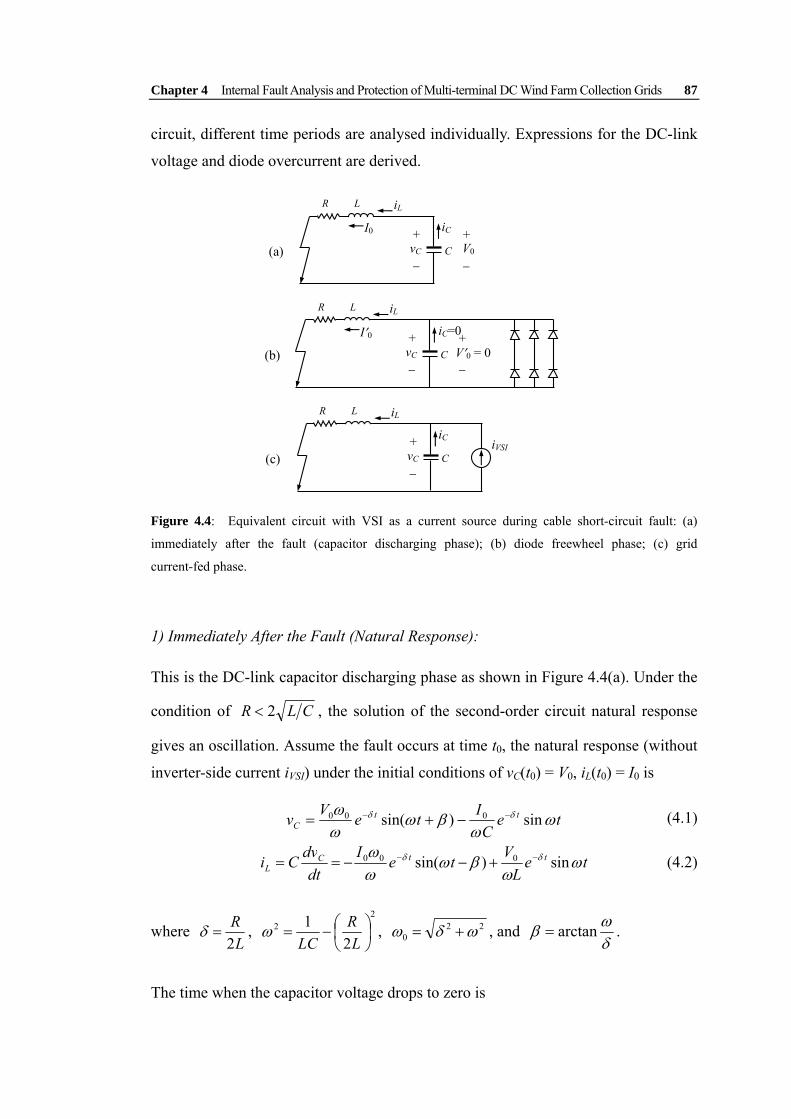
Chapter 4 Internal Fault Analysis and Protection of Multi-terminal DC Wind Farm Collection Grids 87
circuit, different time periods are analysed individually. Expressions for the DC-link
voltage and diode overcurrent are derived.
(a)
iC +
− vC
R iL L
C
I0 +
− V0
(b)
iC=0+
− vC
R iL L
C
I′0 +
− V′0 = 0
(c)
iC +
− vC
R iL L
CiVSI
Figure 4.4: Equivalent circuit with VSI as a current source during cable short-circuit fault: (a)
immediately after the fault (capacitor discharging phase); (b) diode freewheel phase; (c) grid
current-fed phase.
1) Immediately After the Fault (Natural Response):
This is the DC-link capacitor discharging phase as shown in Figure 4.4(a). Under the
condition of CLR 2< , the solution of the second-order circuit natural response
gives an oscillation. Assume the fault occurs at time t0, the natural response (without
inverter-side current iVSI) under the initial conditions of vC(t0) = V0, iL(t0) = I0 is
teC
IteVv ttC ω
ωβω
ωω δδ sin)sin( 000 −− −+= (4.1)
teL
VteIdt
dvCi ttCL ω
ωβω
ωω δδ sin)sin( 000 −− +−−== (4.2)
where L
R2
=δ , 2
2
21
⎟⎠⎞
⎜⎝⎛−=
LR
LCω , 22
0 ωδω += , and δωβ arctan= .
The time when the capacitor voltage drops to zero is

Chapter 4 Internal Fault Analysis and Protection of Multi-terminal DC Wind Farm Collection Grids 88
ωγπ )(01 −+= tt (4.3)
where [ ])cos()sin(arctan 00000 ICVCV −= βωβωγ .
2) Diode Freewheel Stage (After vC = 0, Natural Response):
This is the cable inductor discharging phase which is solved using the first-order
equivalent circuit [Figure 4.4(b)], where the inductor current circulates in the VSI
freewheel diodes. The inductor current has an initial value iL(t1) = I′0. The expression
of inductor discharge current, where each phase-leg freewheel diode current carries a
third of the current, is
iL = I′0 e–(R/L)t, iD1 = iL / 3. (4.4)
This is the most challenging phase for VSI freewheel diodes, because the freewheel
overcurrent is very abrupt with a high initial value, which can immediately damage
the diodes.
3) Grid-Side Current Feeding Stage (Forced Response):
This is the DC-link capacitor and cable inductor under a forced current source
response (with iVSI when the VSI control blocked, vC is not necessarily zero) [Figure
4.4(c)]. To calculate the fault current contribution from the inverter, a three-phase
short-circuit current expression is obtained by three-phase short-circuit analysis. For
phase a, assume the grid voltage after fault occurs is vga = Vgsin(ωst + α), with Vg as
the amplitude, ωs as the synchronous angular frequency, phase-a voltage angle α at t1,
the phase current is
τϕαϕαϕαω tggsgga eIItIi −−−−+−+= )]sin()sin([)sin( 0|0| (4.5)
where ( )RLLchokes )(arctan += ωϕ , RLLchoke )( +=τ , Ig|0| and ϕ0 are the initial
grid current amplitude and phase angle, Lchoke is the grid-side choke inductance.
The positive iga current flows from diode D1 to contribute to the iVSI, with those of igb
and igc, so the total iVSI is the positive three-phase short-circuit current summation
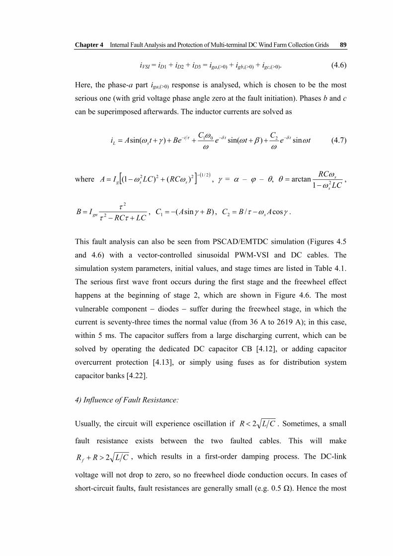
Chapter 4 Internal Fault Analysis and Protection of Multi-terminal DC Wind Farm Collection Grids 89
iVSI = iD1 + iD2 + iD3 = iga,(>0) + igb,(>0) + igc,(>0). (4.6)
Here, the phase-a part iga,(>0) response is analysed, which is chosen to be the most
serious one (with grid voltage phase angle zero at the fault initiation). Phases b and c
can be superimposed afterwards. The inductor currents are solved as
teCteCBetAi tttsL ω
ωβω
ωωγω δδτ sin)sin()sin( 201 −−− +++++= (4.7)
where [ ] ( )2/1222 )()1( −+−= ssg RCLCIA ωω , γ = α – ϕ – θ,
LCRC
s
s21
arctanωωθ
−= ,
LCRCIB gn +−
=ττ
τ2
2
, )sin(1 BAC +−= γ , γωτ cos/2 ABC s−= .
This fault analysis can also be seen from PSCAD/EMTDC simulation (Figures 4.5
and 4.6) with a vector-controlled sinusoidal PWM-VSI and DC cables. The
simulation system parameters, initial values, and stage times are listed in Table 4.1.
The serious first wave front occurs during the first stage and the freewheel effect
happens at the beginning of stage 2, which are shown in Figure 4.6. The most
vulnerable component − diodes − suffer during the freewheel stage, in which the
current is seventy-three times the normal value (from 36 A to 2619 A); in this case,
within 5 ms. The capacitor suffers from a large discharging current, which can be
solved by operating the dedicated DC capacitor CB [4.12], or adding capacitor
overcurrent protection [4.13], or simply using fuses as for distribution system
capacitor banks [4.22].
4) Influence of Fault Resistance:
Usually, the circuit will experience oscillation if CLR 2< . Sometimes, a small
fault resistance exists between the two faulted cables. This will make
CLRR f 2>+ , which results in a first-order damping process. The DC-link
voltage will not drop to zero, so no freewheel diode conduction occurs. In cases of
short-circuit faults, fault resistances are generally small (e.g. 0.5 Ω). Hence the most

Chapter 4 Internal Fault Analysis and Protection of Multi-terminal DC Wind Farm Collection Grids 90
critical phase can sometimes be avoided, only overcurrent protection for the DC-link
capacitor and cables are required. The overcurrent protection relay time setting is not
that critical as well. The damping-only effect will be shown in cable ground fault, in
which the ground resistance is always considerable.
Table 4.1: Simulation Parameters and Calculation Initial Values for Short-Circuit Fault
Simulation system parameters Initial values Times
R = 0.12 Ω V0 = 1.0 kV (DC) t0 = 0 s
L = 0.56 mH I0 = 0.036 kA (DC) t1 = 4.44 ms
C = 10 mF I′0 = 2.619 kA (DC)
Vg = 0.392 kV (AC) 473.0/212.0 =<= CLR
|Z| = |R+jω(Lchoke+L)| =2.691
Lchoke = 8 mH Ig = 0.392/2.691 = 0.146 kA
0 10 20 30 40 50 60 70 80 90 1000
1
2
3
iL (k
A)
0 10 20 30 40 50 60 70 80 90 100-0.5
0
0.5
1
vC (k
V)
0 10 20 30 40 50 60 70 80 90 1000
0.2
0.4
igV
SI (
kA)
0 10 20 30 40 50 60 70 80 90 100-0.5
0
0.5
iga,
b,c
(kA
)
time (ms)
Figure 4.5: VSI with cable short-circuit fault simulation: (a) cable inductor current iL; (b) DC-link
capacitor voltage vC; (c) current provided by grid VSI igVSI; (d) grid side three-phase currents ig a,b,c.
(a)
(b)
(c)
(d)
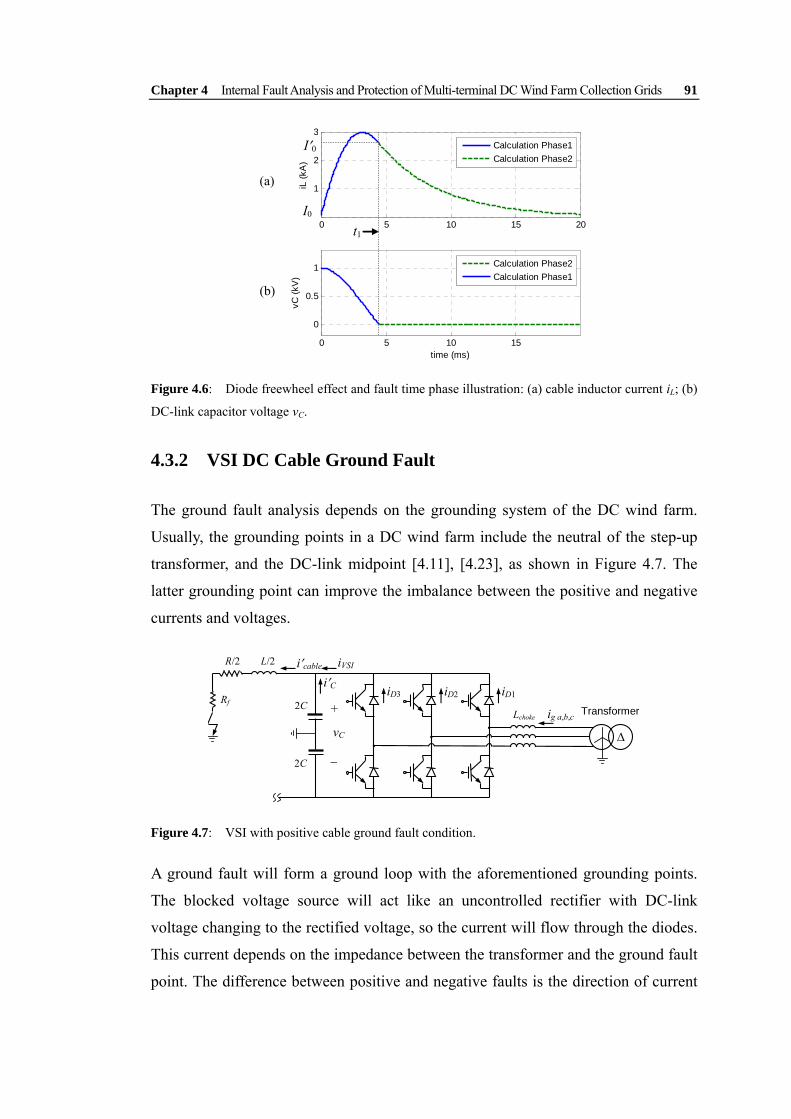
Chapter 4 Internal Fault Analysis and Protection of Multi-terminal DC Wind Farm Collection Grids 91
0 5 10 15 200
1
2
3
iL (k
A)
0 5 10 15
0
0.5
1
vC (k
V)
time (ms)
Calculation Phase1Calculation Phase2
Calculation Phase2Calculation Phase1
t1
I′0
I0
Figure 4.6: Diode freewheel effect and fault time phase illustration: (a) cable inductor current iL; (b)
DC-link capacitor voltage vC.
4.3.2 VSI DC Cable Ground Fault
The ground fault analysis depends on the grounding system of the DC wind farm.
Usually, the grounding points in a DC wind farm include the neutral of the step-up
transformer, and the DC-link midpoint [4.11], [4.23], as shown in Figure 4.7. The
latter grounding point can improve the imbalance between the positive and negative
currents and voltages.
iD3 iD2 iD1
ig a,b,c
iVSI i′C
+
−
vC
R/2 i′cable L/2
2C Lchoke
2C
Δ
Rf Transformer
Figure 4.7: VSI with positive cable ground fault condition.
A ground fault will form a ground loop with the aforementioned grounding points.
The blocked voltage source will act like an uncontrolled rectifier with DC-link
voltage changing to the rectified voltage, so the current will flow through the diodes.
This current depends on the impedance between the transformer and the ground fault
point. The difference between positive and negative faults is the direction of current
(a)
(b)

Chapter 4 Internal Fault Analysis and Protection of Multi-terminal DC Wind Farm Collection Grids 92
and the bridge diodes that conduct. The fault resistance Rf cannot be ignored in this
case, usually ground fault resistance varies from ohms to hundreds of ohms [4.6].
The equivalent circuit is shown in Figure 4.8 for the fault calculation, which is
divided into transient and steady phases.
(a) i′C +
− v′C
R′ i′cableL′
C ′
I0 +
− V′0
Rf
(b)
i′C +
−
R′ i′cableL′
C ′
I0 +
− V′0
Rf
vg a,b,c ~ ~ ~
Lchoke
ig a,b,c
v′C < vg a,b,c
Figure 4.8: Equivalent circuit for the VSI with a cable ground fault calculation: (a) stage 1 –
capacitor discharge; (b) stage 2 – grid current feeding.
1) Capacitor Discharge Stage (Natural Response):
This is the DC-link capacitor discharging stage as represented by Figure 4.8(a).
Under the condition of CLRRf ′′>′+ 2 , the solution of the second-order circuit
natural response gives a non-oscillating discharge process. The DC-link voltage will
not drop to zero so no freewheel diode conduction occurs. Assume the fault happens
at time t0, the natural response (without inverter side current iVSI) under initial
conditions of v′C(t0) = V0, i′cable(t0) = I0 are
tptpC eAeAv 21
21 +=′ (4.8)
tptpCcable epAepA
dtvdCi 21
2211 +=′
′=′ (4.9)
where CLL
RRL
RRp ff
′′−⎟⎟
⎠
⎞⎜⎜⎝
⎛′
′+±
′
′+−=
122
2
2,1 , ⎟⎠⎞
⎜⎝⎛
′+
−=
CIVp
ppA 0
0212
11 ,
⎟⎠⎞
⎜⎝⎛
′−−
−=
CIVp
ppA 0
0112
21 .
Chapter 4 Internal Fault Analysis and Protection of Multi-terminal DC Wind Farm Collection Grids 93
This stage is an RLC circuit until the positive DC voltage drops to below any grid
phase voltage. It is difficult to determine an analytical expression for the time t1
when capacitor voltage drops below any grid phase voltage but numerical methods
can be used to find the time solution.
2) Grid Side Current Feeding Stage (Forced Response):
This transient phase can be expressed by third-order state-space equations
cbag
chokeL
cable
C
choke
f
L
cable
C
vLi
iv
L
LRR
L
CC
iiv
chokechoke
,,
100
001
01
110
⎟⎟⎟
⎠
⎞
⎜⎜⎜
⎝
⎛+
⎟⎟⎟
⎠
⎞
⎜⎜⎜
⎝
⎛′′
⎟⎟⎟⎟⎟⎟⎟
⎠
⎞
⎜⎜⎜⎜⎜⎜⎜
⎝
⎛
−
′
′+−
′
′′−
=⎟⎟⎟
⎠
⎞
⎜⎜⎜
⎝
⎛′′
&
&
&
(4.10)
where Cv′ , i′cable, and chokeLi are the state variables. The choke inductance can also
include the transformer and its star-grounding inductance in case of an
arc-distinguishing coil connected in low or medium voltage situations. It is difficult
to derive analytical expressions for the voltages and currents during the fault so it is
numerically simulated. There are no particular effects on the diodes (unlike the
freewheel phase during short-circuits). The capacitor voltage drops to a new steady
state in 30 milliseconds; meanwhile the inductor current experiences a large transient
of 0.8 kA (11 times rated current), Figure 4.9(a).
It cannot be solved continuously because of commutation between diodes. Therefore,
for each diode conduction period, the status equations of (4.10) need to be solved
using the previous variable as the initial state for the present calculation.
3) Steady State:
The steady-state equations can be determined. The total impedance is
θωωω ′∠=+++= ZLjCjLjRRZ chokesssf )/1()( (4.11)
Then the current through diode is
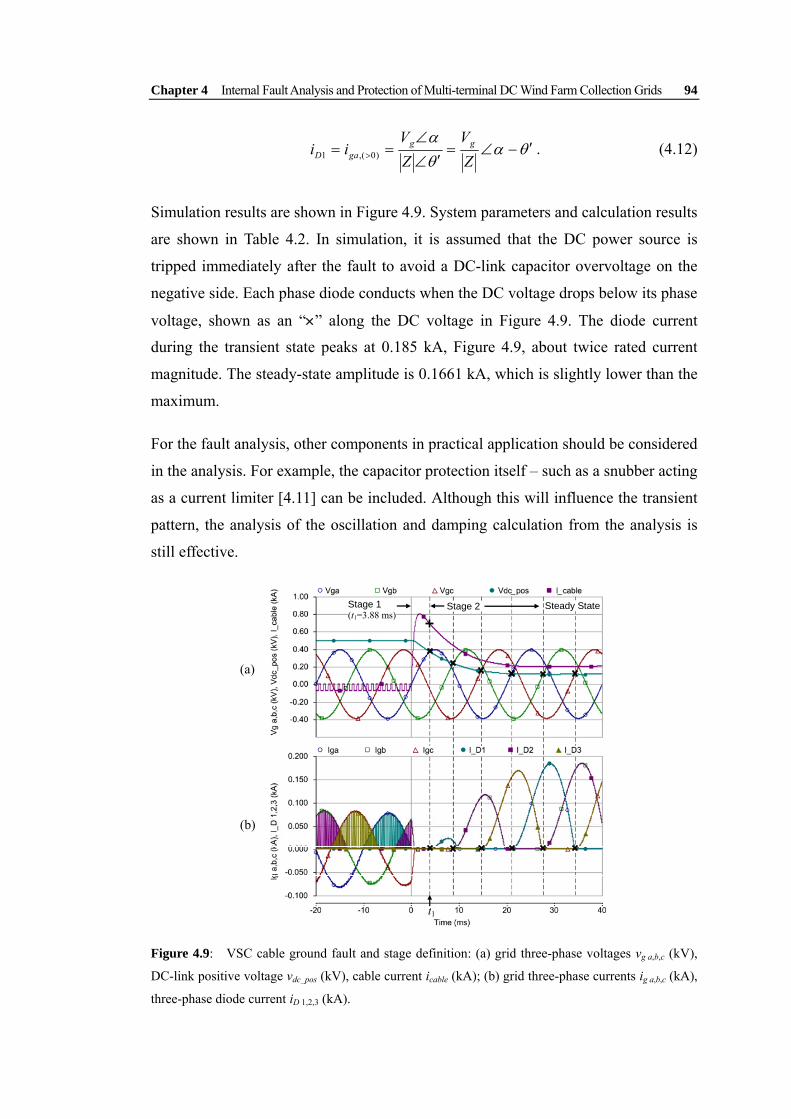
Chapter 4 Internal Fault Analysis and Protection of Multi-terminal DC Wind Farm Collection Grids 94
θαθα
′−∠=′∠
∠== > Z
VZV
ii gggaD )0(,1 . (4.12)
Simulation results are shown in Figure 4.9. System parameters and calculation results
are shown in Table 4.2. In simulation, it is assumed that the DC power source is
tripped immediately after the fault to avoid a DC-link capacitor overvoltage on the
negative side. Each phase diode conducts when the DC voltage drops below its phase
voltage, shown as an “×” along the DC voltage in Figure 4.9. The diode current
during the transient state peaks at 0.185 kA, Figure 4.9, about twice rated current
magnitude. The steady-state amplitude is 0.1661 kA, which is slightly lower than the
maximum.
For the fault analysis, other components in practical application should be considered
in the analysis. For example, the capacitor protection itself – such as a snubber acting
as a current limiter [4.11] can be included. Although this will influence the transient
pattern, the analysis of the oscillation and damping calculation from the analysis is
still effective.
Stage 1 (t1=3.88 ms)
Stage 2 Steady State
t1
Figure 4.9: VSC cable ground fault and stage definition: (a) grid three-phase voltages vg a,b,c (kV),
DC-link positive voltage vdc_pos (kV), cable current icable (kA); (b) grid three-phase currents ig a,b,c (kA),
three-phase diode current iD 1,2,3 (kA).
(a)
(b)

Chapter 4 Internal Fault Analysis and Protection of Multi-terminal DC Wind Farm Collection Grids 95
Table 4.2: Simulation Parameters and Calculation for Ground Fault
Simulation system parameters Initial / Calculation values Times
R ′ = R/2 = 0.06 Ω, Rf = 0.5 Ω V0 = 0.5 kV (DC) t0 = 0 s
L ′ = L/2 = 0.28 mH I0 = -0.063 kA (DC) t1 = 3.88 ms
C ′ = 2C = 20 mF Vg = 0.392 kV (AC)
237.0/256.0 =′′>=′+ CLRR f Z = 2.36∠88.96°
Lchoke = 8 mH Ig = 0.1661 kA (AC)
4.3.3 DC Cable Open-Circuit Fault
Open-circuit faults will only influence generator-side converters but not grid-side
converters, although this can influence the online AC grid system because of the
abrupt generation loss. The disruption of energy transmission path means that
redundant energy generated by the turbine-generator system will cause overvoltage
behind the rectifier and generator acceleration and overspeed. This can be solved by
applying the dump load at the generator AC side or a DC-chopper after the rectifier
to limit the rectified DC overvoltage. Energy storage systems (ESS) could also be
used at the rectifier DC-link [4.24].
4.3.4 Multi-level Voltage-Source Converters
The fault analysis is applied to the common multi-level converters. Three-level diode
neutral-point-clamp (3L-NPC) converter and five-level flying capacitor (5L-FC)
converter are illustrated for cable ground fault and short-circuit fault, respectively
(Figure 4.10). From the topology, the above two-level analysis remains effective for
them as the main characteristics remain: a closed loop for capacitance discharge via
freewheel diodes.
The diodes share short-circuit fault current, in Figure 4.10(a), except that during the
first stage D1 carries more current due to the discharge of capacitor C2. The ground
fault with clamping diodes form a freewheel loop when v′C drops to zero, shown as
dashed line in Figure 4.10(b), just like the second stage of the above short-circuit
fault. Hence the short-circuit fault analysis can be applied to this situation. For

Chapter 4 Internal Fault Analysis and Protection of Multi-terminal DC Wind Farm Collection Grids 96
cascaded modular multi-level converters, each cell has its own capacitor. There is no
large capacitance across the DC-link, therefore, no discharge current under a DC
short-circuit fault. Protection control and fast switching within each cell make this
topology tolerant to short-circuit faults. However, during the DC network
development with all kinds of VSCs, it is not possible to build a system with these
fault-tolerant converters only. Hence it is still necessary to analyse and provide
system protection as a whole.
iDp
A
iVSI
iC1 +
−
vC1
R/2 icable L/2 P
N
D1
C1 C2
iC2
iDp
A
iVSI
iC +
−
v′C
R/2 L/2
2C
P
2C
Rf
iDc
N
i′cable
(a) (b)
Figure 4.10: Multi-level VSC fault condition illustration: (a) five-level flying-capacitor converter
under cable short-circuit fault; (b) three-level diode neutral-point-clamp converter under cable ground
fault.
4.3.5 Fault Characteristic Summary
The DC-link voltage change can be used to separate AC faults from DC faults. For
AC faults, the redundant energy that cannot be transferred to grid is stored in
DC-link capacitor and results in the increase of DC-link voltage. But for inner DC
faults, the DC-link voltage will collapse. In Table 4.3, fault overcurrent is
characterised in three aspects: 1) initial current change, 2) first wave rise-time, and 3)
oscillation pattern, which can all be used for identification and detection of fault
type.

Chapter 4 Internal Fault Analysis and Protection of Multi-terminal DC Wind Farm Collection Grids 97
Table 4.3: Fault Characteristic Summary
Fault type AC faults Short-circuit Ground-fault Open-circuit
Direction of DC-link voltage change ↑ ↓ ↓ ↓
Initial current change ⎯ Up to 73 times of
rating Up to 11 times of
rating ⎯
Rise-time of first wave front ⎯ < 5 ms > 0.25(1/fs) = 5 ms ⎯
DC side fault
current Oscillation
pattern ⎯ RLC discharging,
RL diode freewheel
Sinusoidal ⎯
fs − the synchronous time frequency.
4.4 DC Fault Protection Methods
The aforementioned DC fault analysis and detection can be applied to the design of
the protection system. The main principles are the same with AC distribution system
protection: time-response, selectivity, and reliability. There are few published works
on DC system protection with a DC CB and relay configuration. Most reported
methods avoid using DC CBs, because of the lag in development and cost. Moreover,
no relay experience can be gained from the traditional HVDC systems. In most cases,
the DC faults discussed here have similar characteristics to the DC-link voltage
collapse but with different amplitudes of overcurrent. Hence, overcurrent protection
with a directional element can realise fault location without communication between
the two switchgears at the terminals of a long cable. The selectivity can be realised
by using relay time delay or time coordination curves.
4.4.1 DC Switchgear
There are some options for switchgear: 1) AC CB and DC Switch: AC-side CBs are
used for fault current extinguishing, coordinating with DC fast switches [4.15]; 2) DC
CB: fully-functioned DC CB − the optimal option; 3) fuse: used for systems that only
require fast response for protection and no need to reenergise the system automatically.
Fuses could be used at each generator’s converter output side as shown in Figure 4.1.
Considering the strict time-response requirement, AC CBs will not be suitable.

Chapter 4 Internal Fault Analysis and Protection of Multi-terminal DC Wind Farm Collection Grids 98
DC circuit breakers are required for the collection and transmission systems as they
require fast response under DC fault conditions. The AC side breaker and DC switch
coordination obviously cannot function fast enough; when the fault occurs, the
mechanical arc-extinguishing AC side breakers operation time cannot avoid the
diode freewheel effect analysed above, hence is not capable of fast fault clearance.
Moreover, the allocation of DC breakers can enhance the system reliability,
especially for the loop network topology, in which the AC-side breakers and DC
switches can only be used for a “cut-and-try” method as proposed in [4.15]. Detailed
design of DC CBs and appropriate fuse selection is required to satisfy issues such as
effective arc-extinguishing and fault clearance. This is a significant challenge for DC
switchgear design.
4.4.2 Measurement and Relaying Configuration
The main protection should operate as fast as possible, with one backup protection,
operating after a time delay in case the main protection malfunctions. However, the
backup protection still needs to be fast enough to avoid the freewheel effect, which is
less than 5 ms in the aforementioned example. Therefore, the protection time
response should be at the millisecond level, depending on the protection coordination
(selection) method. Distance protection is usually applied. The main principle is to
estimate the impedance between the relay point and the fault point. If this falls within
a given distance, the relay system waits for a corresponding time delay before
activation to realise selection.
1) Communication Solution:
If each cable section is not too long, the relay detecting opposite current flow will
communicate with its former relay. If their current directions are the same, then the
fault has occurred outside this section. The relay will wait for a delay time. If the
correct directions are different, the fault is between the relays and this relay operates
immediately. Since there is no further CB at the terminal of a string or star, the CB at
this relay point will trip instantly. If all the relay delay times are exceeded and there
is still overcurrent, the circuit breaker will trip as backup protection.

Chapter 4 Internal Fault Analysis and Protection of Multi-terminal DC Wind Farm Collection Grids 99
2) Distance Evaluation Solution:
Traditional AC system distance protection uses impedance to represent the distance
from fault point to the relay point. The distance judgement is made with mho
characteristic or an impedance circle. But for DC systems and during fault transients,
the frequency changes abruptly, so no grid fundamental frequency impedance can be
defined for distance protection. In three-phase AC systems, distance protection uses
symmetrical component analysis to avoid the influence of fault resistance [4.6].
However, in DC systems, this is not possible. A new distance evaluation solution is
proposed.
For a fast time-response protection system, if the main protection and backup
coordination are capable of securely protecting the system, at the protection stage,
there is no need to use time-consuming methods to accurately locate the distance to
the fault point. Rough distance evaluation is enough for a relay decision. This relies
on the distance characteristics of overcurrent value and critical time for the freewheel
effect. The DC-link voltage and cable inductor current variation to different fault
distances are shown in Figure 4.11, where D is the cable length of one section. As the
distance increases, the fault overcurrent reduces and the time-to-peak current
increases.
(a)
5 10 15 20 25 30 35 40 45 50
-0.5
0
0.5
1
vc (k
V)
D2D4D
(b)
0 5 10 15 20 25 30 35 40 45 50
-1
0
1
2
3
iL (k
A)
time (ms)
D2D4D
Figure 4.11: Influence of fault distance on the system performance: (a) DC-link capacitor voltages
of difference distances; (b) cable inductor currents of different distances.

Chapter 4 Internal Fault Analysis and Protection of Multi-terminal DC Wind Farm Collection Grids 100
The critical time limit is when the DC-link voltage drops to zero as in Figure 4.11(a).
At this time, the freewheel diodes conduct. With respect to the distance x, the critical
time is
( )[ ] ωδωπ ′−′−=− )(arctan 00001 ICVCVtt (4.13)
where 220 δωω −=′ x . (4.14)
The freewheel overcurrent is the cable inductor current at the critical time. The
critical freewheel current and time with respect to distance is shown in Figure 4.12.
The critical time is the strict upper limit for the total switchgear operation time. The
current-distance curve in Figure 4.12(a) can be used for relay configuration.
Examples are shown in Figure 4.13. t(n) is the relay time delay curve at point (n).
Here, the critical time is used to coordinate the delay time of the relays, shown in
Figure 4.13(a), which is easier to apply than the Figure 4.13(b) method.
(a)
0 0.5 1 1.5 2 2.5 3 3.5 4
0
5
10
15
20
iL (k
A)
(b)
0 0.5 1 1.5 2 2.5 3 3.5 4
0
5
10
15
t crit
ical
(ms)
distance (km)
Figure 4.12: Influence of fault distance on the system performance: (a) initial freewheel current
according to the fault distance; (b) DC-link capacitor voltage collapse time change with distance.
(Each cable section can be 1 km long.)
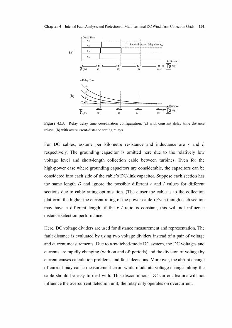
Chapter 4 Internal Fault Analysis and Protection of Multi-terminal DC Wind Farm Collection Grids 101
(a)
(1) (2) (3) (4) (flt)
t(4)
t(3)
t(2)
t(1)
Distance
Standard section delay time tsd
VSI
Delay Time
(b)
(1) (2) (3) (4)
t(4)
t(3)
t(2) t(1)
(flt)
Distance
VSI
Delay Time
Figure 4.13: Relay delay time coordination configuration: (a) with constant delay time distance
relays; (b) with overcurrent-distance setting relays.
For DC cables, assume per kilometre resistance and inductance are r and l,
respectively. The grounding capacitor is omitted here due to the relatively low
voltage level and short-length collection cable between turbines. Even for the
high-power case where grounding capacitors are considerable, the capacitors can be
considered into each side of the cable’s DC-link capacitor. Suppose each section has
the same length D and ignore the possible different r and l values for different
sections due to cable rating optimisation. (The closer the cable is to the collection
platform, the higher the current rating of the power cable.) Even though each section
may have a different length, if the r−l ratio is constant, this will not influence
distance selection performance.
Here, DC voltage dividers are used for distance measurement and representation. The
fault distance is evaluated by using two voltage dividers instead of a pair of voltage
and current measurements. Due to a switched-mode DC system, the DC voltages and
currents are rapidly changing (with on and off periods) and the division of voltage by
current causes calculation problems and false decisions. Moreover, the abrupt change
of current may cause measurement error, while moderate voltage changes along the
cable should be easy to deal with. This discontinuous DC current feature will not
influence the overcurrent detection unit; the relay only operates on overcurrent.

Chapter 4 Internal Fault Analysis and Protection of Multi-terminal DC Wind Farm Collection Grids 102
The measurements and distance relationship are illustrated in Figure 4.14. The fault
voltage at switchgear relay point (n) is
⎟⎟⎠
⎞⎜⎜⎝
⎛++=++=
dtdi
lrixiRdt
dilxrixvv n
nfltfn
nfltn)(
)(*
)()(*
)(*
)()( (4.15)
where x* is the real fault distance and Rf is the fault resistance.
vm(n) vm(r)
x*
(flt) (n)
Rf
d (r) i(n)
i(flt)
Figure 4.14: Distance evaluation with two voltage divider measurements.
Another relay voltage sensor unit (r) is used as a reference for the relative voltage
calculation; it is located close to the main relay point on the same section of cable, as
shown in Figure 4.14 to avoid long-distance communication issues. The measured
values using voltage dividers are vm(n) = kvv(n) and vm(r) = kvv(r), where kv is the voltage
divider ratio. The distance between them is known d, so the fault distance measured
from this reference is
dvv
vd
vvv
xrmnm
nm
rn
n
)()(
)(
)()(
)(
−=
−= (4.16)
where ⎟⎟⎠
⎞⎜⎜⎝
⎛+=−
dtdi
lridvv nnrn
)()()()( . (4.17)
For metallic grounding or a short-circuit fault, v(flt) = Rf i(flt) = 0, so the cable
impedance is proportional to the distance. Measured distance x = x* can be used for
the distance relay configuration. If the distance calculation is within a given section,
the relay will operate with a corresponding time delay to realise selection as shown
in Figure 4.13(a). The delay time of all the sections should be less than the critical
time to avoid freewheel diode overcurrent.
Chapter 4 Internal Fault Analysis and Protection of Multi-terminal DC Wind Farm Collection Grids 103
For high resistance faults, which are more common in ground faults, the existence of
Rf and the difference between i(flt) and i(n) make the evaluation of x* difficult. Usually,
this kind of fault is not as serious as the metallic grounding or short circuit, so it may
not require fast time-response protection, hence it can be fulfilled by the overcurrent
setting. Considering the backup configuration and the critical time limit shown in
Figure 4.12(b), a method to estimate the fault distance is proposed by estimating the
cable distance and equivalent fault resistance.
The distance measured in (4.16) in this case is not accurate because of the influence
of fault resistance, but this is the only information that can be used for time delay
decision. Equation (4.17) presents the real voltage drop between the two relay points,
which reflects the real voltage drop excluding the influence of Rf i(flt). But Rf still
cannot be exactly obtained even with the source side tripped (i.e. i(flt) = i(n)). One
solution is to measure the reactance to exclude the resistance influence, but this is
hard to achieve. Under the assumption that the DC power source side is immediately
tripped, the voltage measurement is
( )KrixiRdt
dilrixiRv nnf
nnnfn ++=⎟⎟
⎠
⎞⎜⎜⎝
⎛++= 1)(
*)(
)()(
*)()( (4.18)
where ( ))()(
nn ri
dtdi
lK ⎟⎟⎠
⎞⎜⎜⎝
⎛= (4.19)
is the equivalent ratio of reactance to resistance voltage drops. Then defining
)1()()(
)( KDridt
dilriDR n
nnD +=⎟⎟
⎠
⎞⎜⎜⎝
⎛+= (4.20)
as the equivalent resistance per section. Hence, the measured distance
( ) *
)()(
)(*
)(
)()(
)( 1xD
RR
dtdi
lri
KrixiRd
vvv
xD
f
nn
nnf
rn
n +=
⎟⎟⎠
⎞⎜⎜⎝
⎛+
++=
−= . (4.21)
In practical applications, it is not economical to allocate CBs at each collection unit
end in a collection string. For a string with ten turbines, the total number of CBs can

Chapter 4 Internal Fault Analysis and Protection of Multi-terminal DC Wind Farm Collection Grids 104
be 3 or 4, so the delay time will be about 4.44/4 ms in the aforementioned case. This
requires the DC CBs to operate at a 1-ms level, which is achievable. The evaluation
decision procedure is shown in the distance estimation table (Table 4.4), used for
coordination, to allocate main protection and backup protection. The standard section
delay time tsd for coordination is calculated according to the critical time divided by
the corresponding section number.
Table 4.4: Distance Protection Relay Time Coordination for a 3-Section Example
Relay Fault distance
Fault region
Fault resistance
Confidence in Discrimination
Switch Delay
x ≤ D (1)-(0) -- Yes 0 (1)
x > D (1)-(0) Rf > 0 Yes 0
x ≤ D (2)-(1) -- Yes 0 (2)-(1) Rf ≥ RD D < x ≤
2D (1)-(0) 0 ≤ Rf < RD No tsd
(2)-(1) Rf ≥ 2RD
(2)
x > 2D (1)-(0) 0 ≤ Rf < RD
No 2tsd
x < D (3)-(2) -- Yes 0 (3)-(2) Rf ≥ RD D < x ≤
2D (2)-(1) 0 ≤ Rf < RD No tsd
(3)-(2) Rf ≥ 3RD (2)-(1) RD ≤ Rf < 2RD
2D < x ≤ 3D
(1)-(0) 0 ≤ Rf < RD
No 2tsd
(3)-(2) Rf ≥ 3RD (2)-(1) RD ≤ Rf < 2RD
(3)
x > 3D (1)-(0) 0 ≤ Rf < RD
No 3tsd
A three-section example is shown in Table 4.4. For the relay (1) at the far end of a
string cable, the measured distance only falls into two conditions. Regardless of what
is the measured x value is, the CB will immediately operate when overcurrent is
detected. For relay (2), if x ≤ D, it is certain that the fault occurred inside the cable
between (2) and (1), so the delay time is also 0. But if x > D, whether it is smaller
than 2D, it is hard to decide whether cable (2)-(1) or (1)-(0) is faulted. But the bigger
the evaluated distance x is, the less serious the fault is, so the time delay is set as a
backup standard, with one tsd delay or 2tsd delay when x > 2D. The closer the relay is
to the inverter, the greater the possibilities are to assess, and the longer the time is
available, for distance measurement. The evaluation procedure using different

Chapter 4 Internal Fault Analysis and Protection of Multi-terminal DC Wind Farm Collection Grids 105
distance calculation values to set relay delay times is to distinguish the main and
backup protections. This ensures that the fault is cleared by at least the backup
protection.
4.4.3 Small-Scale System Protection Option
A simple method is proposed for small-scale, low-power scenarios. Reverse diodes
can be used to restrain the fault current from flowing into the DC cable system. The
VSI diodes clamp the voltage after the DC-link capacitor, another pair of diodes can
be used before the DC-link to block the fault current flowing in the other direction.
In this way, the DC-link voltage will not change abruptly. The DC-chopper circuit is
used in case of DC-link overvoltage. The reverse diode positions and current flows
are shown in Figure 4.15.
VSI
T,p-g
T,n-g
T,p-n
DC-Chopper
Reverse Diode iVSI
vC−
+
Figure 4.15: Reverse-diode protection method and current flow directions.
PSCAD/EMTDC simulations are carried out. The simulated system topology is a DC
wind farm collection grid with diode-rectifier and DC/DC boost conversion in
parallel with the grid-side VSI. This is economical and practical for small-scale
systems. The simulated DC wind farm system includes two equivalent
parallel-connected wind turbine generation systems. The faults simulated are: 1) a
short-circuit fault for 1.0 s and 2) a cable ground fault for 1.0 s. Both occur on the
cable of one generation system. Zero fault resistance is considered to give the most
serious condition.
The DC-link capacitor voltage and inverter-side reverse currents are shown in Figure
4.16. For a short-circuit fault, the DC-link voltage is clamped to be around the
pre-fault value and no current flows through the diodes to charge the capacitor [i.e.,
the inverter current is almost zero in Figure 4.16(b)], compared with that of up to

Chapter 4 Internal Fault Analysis and Protection of Multi-terminal DC Wind Farm Collection Grids 106
2.50 kA in Figure 4.16(a). The overvoltage after the recovery of fault will be reduced
by the DC-chopper. For a ground-fault condition, no DC-chopper is needed. There is
an inverter overcurrent, but this is limited to twice of the normal value, which is
tolerable for devices.
(a)
1.50 2.00 2.50 3.00 3.50 4.00 -0.50 0.00 0.50 1.00 1.50 2.00 2.50
vC (kV) IVSI (kA)
(b)
1.50 2.00 2.50 3.00 3.50 4.00 -0.20 0.00 0.20 0.40 0.60 0.80 1.00 1.20
vC (kV) iVSI (kA)
(c)
1.50 2.00 2.50 3.00 3.50 4.00 -0.50 -0.25 0.00 0.25 0.50 0.75 1.00 1.25 1.50
vC (kV) iVSI (kA)
(d)
Time (s)1.50 2.00 2.50 3.00 3.50 4.00
-0.20 0.00 0.20 0.40 0.60 0.80 1.00 1.20
vC (kV) iVSI (kA)
Figure 4.16: Reverse-diode and DC-chopper protection method performance (DC-link capacitor
voltage vC and VSI current iVSI) simulation: (a) short-circuit fault without protection; (b) short-circuit
fault with protection; (c) cable ground fault without protection; (d) cable ground fault with protection.
4.5 DC Wind Farm Protection Simulation Results
The proposed protection method is applied to specific DC wind farm systems and
verified by PSCAD/EMTDC simulations. The topologies investigated are small-scale
DC wind farm collection grids with star and string connections, respectively. The
generators are PMSGs. The generator-side AC/DC converters are three-phase

Chapter 4 Internal Fault Analysis and Protection of Multi-terminal DC Wind Farm Collection Grids 107
diode-rectifiers connected to boost DC/DC converters for energy conversion and
maximum power point tracking. The simulated DC wind farm system includes two
equivalent wind turbine generation systems, parallel-connected, to the DC-link and
grid-side inverter. The faults simulated are: 1) for the star connection, a short-circuit
fault on the cable of one collection unit; 2) for the string connection, a grounding
fault on the collection cable of one unit is close to the inverter side. The generator
and DC cable parameters are provided in Table 4.5 and 4.6.
Table 4.5: PMSG Parameters
Parameter Value Parameter Value
Rated power Pn 25 kW Pole pair no. Pp 12
Rated stator voltage Vsn 450 V Phase resistance 0.068 p.u.
Rated frequency fg 30 Hz Phase inductance 0.427 p.u.
Table 4.6: DC Cable Parameters
Parameter Value Parameter Value Resistance r 0.06 Ω/km Collection cable (1)-(0) 0.5 km
Inductance l 0.28 mH/km Collection cable (2)-(0) for star / (2)-(1) for string
0.5 km
Rating voltage 1 kV Transmission cable (3)-(2) 1.0 km
4.5.1 Short-Circuit Fault Condition
Figure 4.17 shows the system performance under a short-circuit fault at t = 3.0 s at
the midpoint of one collection cable of a generation system. To show the selection
validity, this fault is applied to the star connected system and the fault point is on one
collection unit cable. The selectivity should make sure this fault will not influence
the power transferred to the inverter from the other turbine system. The protection
opens the faulted side CB immediately. The total power transmitted to the onshore
grid drops to 0.5 p.u. The VSI control maintains the DC-link voltage constant with a
slight transient, Figure 4.17(a). In Figure 4.18, the currents at the two relay points
show that under voltage control, the current at the grid switchgear relay point (3) i(3)
drops to a half due to the trip of CB (1) (i(1) = 0); hence, the total power decreases by
half.
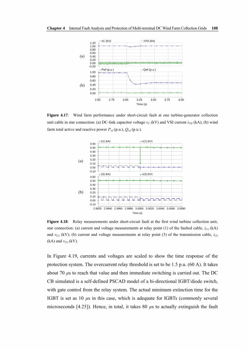
Chapter 4 Internal Fault Analysis and Protection of Multi-terminal DC Wind Farm Collection Grids 108
Time (s)2.50 2.75 3.00 3.25 3.50 3.75 4.00
-0.20 0.00 0.20 0.40 0.60 0.80 1.00 1.20
vC (kV) iVSI (kA)
0.00 0.20 0.40 0.60 0.80 1.00
Pwf (p.u.) Qwf (p.u.)
Figure 4.17: Wind farm performance under short-circuit fault at one turbine-generator collection
unit cable in star connection: (a) DC-link capacitor voltage vC (kV) and VSI current iVSI (kA); (b) wind
farm total active and reactive power Pwf (p.u.), Qwf (p.u.).
Time (s)2.9920 2.9940 2.9960 2.9980 3.0000 3.0020 3.0040 3.0060 3.0080
-0.10 0.00 0.10 0.20 0.30 0.40 0.50 0.60
i(1) (kA)
-0.10 0.00 0.10 0.20 0.30 0.40 0.50 0.60
i(3) (kA)
v(1) (kV)
v(3) (kV)
Figure 4.18: Relay measurements under short-circuit fault at the first wind turbine collection unit, star connection: (a) current and voltage measurements at relay point (1) of the faulted cable, i(1) (kA) and v(1) (kV); (b) current and voltage measurements at relay point (3) of the transmission cable, i(3) (kA) and v(3) (kV).
In Figure 4.19, currents and voltages are scaled to show the time response of the
protection system. The overcurrent relay threshold is set to be 1.5 p.u. (60 A). It takes
about 70 µs to reach that value and then immediate switching is carried out. The DC
CB simulated is a self-defined PSCAD model of a bi-directional IGBT/diode switch,
with gate control from the relay system. The actual minimum extinction time for the
IGBT is set as 10 µs in this case, which is adequate for IGBTs (commonly several
microseconds [4.25]). Hence, in total, it takes 80 µs to actually extinguish the fault
(a)
(b)
(a)
(b)
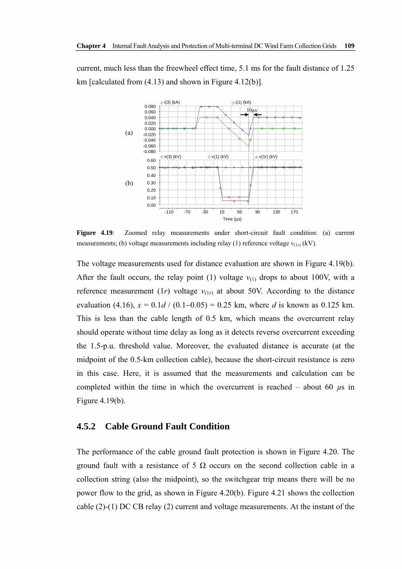
Chapter 4 Internal Fault Analysis and Protection of Multi-terminal DC Wind Farm Collection Grids 109
current, much less than the freewheel effect time, 5.1 ms for the fault distance of 1.25
km [calculated from (4.13) and shown in Figure 4.12(b)].
Time (µs)-110 -70 -30 10 50 90 130 170
-0.080 -0.060 -0.040 -0.020 0.000 0.020 0.040 0.060 0.080
i(1) (kA)
0.00
0.10
0.20 0.30
0.40
0.50
0.60 v(3) (kV) v(1) (kV) v(1r) (kV)
i(3) (kA)
10µs
Figure 4.19: Zoomed relay measurements under short-circuit fault condition: (a) current measurements; (b) voltage measurements including relay (1) reference voltage v(1r) (kV).
The voltage measurements used for distance evaluation are shown in Figure 4.19(b).
After the fault occurs, the relay point (1) voltage v(1) drops to about 100V, with a
reference measurement (1r) voltage v(1r) at about 50V. According to the distance
evaluation (4.16), x = 0.1d / (0.1−0.05) = 0.25 km, where d is known as 0.125 km.
This is less than the cable length of 0.5 km, which means the overcurrent relay
should operate without time delay as long as it detects reverse overcurrent exceeding
the 1.5-p.u. threshold value. Moreover, the evaluated distance is accurate (at the
midpoint of the 0.5-km collection cable), because the short-circuit resistance is zero
in this case. Here, it is assumed that the measurements and calculation can be
completed within the time in which the overcurrent is reached – about 60 µs in
Figure 4.19(b).
4.5.2 Cable Ground Fault Condition
The performance of the cable ground fault protection is shown in Figure 4.20. The
ground fault with a resistance of 5 Ω occurs on the second collection cable in a
collection string (also the midpoint), so the switchgear trip means there will be no
power flow to the grid, as shown in Figure 4.20(b). Figure 4.21 shows the collection
cable (2)-(1) DC CB relay (2) current and voltage measurements. At the instant of the
(a)
(b)

Chapter 4 Internal Fault Analysis and Protection of Multi-terminal DC Wind Farm Collection Grids 110
fault, t = 3.0 s, the current direction is opposite; it feeds current into the fault.
Although the direction element can detect the fault current direction change, the
overcurrent threshold 1.5 p.u. is not reached, so no trip occurs until the delay time
has passed. The evaluated fault distance includes the influence of fault resistance,
hence it is possible to misjudge the fault location. The fault resistance can restrict the
overcurrent so it is not as severe as metallic fault conditions. The time delay is set as
calculated from the fault distance and delay time concept. The evaluated distance
value of relay (2) x is intolerable now (an unreasonably large value, much larger than
the total collection length – 1 km) because of the high fault resistance. So the time
delay of (2) is set to be that for 1 km – 4.44 ms in Figure 4.21, and that of (3) is the
total value of critical time for the entire 2-km cable – 6.89 ms. Figure 4.22 shows the
CB switch timing at relay point (2).
Time (s)2.50 2.75 3.00 3.25 3.50 3.75 4.00
-0.20 0.00 0.20 0.40 0.60 0.80 1.00 1.20
vC (kV) iVSI (kA)
-0.20 0.00 0.20 0.40 0.60 0.80 1.00
Pwf (p.u.) Qwf (p.u.)
Figure 4.20: Wind farm performance under cable ground fault at the second turbine-generator
collection unit cable in string connection: (a) DC-link capacitor voltage vC (kV) and VSI current iVSI
(kA); (b) wind farm total active and reactive power Pwf (p.u.), Qwf (p.u.).
Time (s)
2.9940 2.9960 2.9980 3.0000 3.0020 3.0040 3.0060 3.0080 3.0100 3.0120 -0.20 -0.10 0.00 0.10 0.20 0.30 0.40 0.50 0.60
v(2) (kV)i(2) (kA)
Figure 4.21: Relay measurements under cable ground fault condition, at the relay point (2), current
i(2) (kA) and voltage v(2) (kV).
(a)
(b)

Chapter 4 Internal Fault Analysis and Protection of Multi-terminal DC Wind Farm Collection Grids 111
Time (µs)4320 4360 4400 4440 4480 4520 4560 4600
-0.0300 -0.0250 -0.0200 -0.0150 -0.0100 -0.0050 0.0000 0.0050 0.0100
i(2) (kA)
-0.10 0.00 0.10 0.20 0.30 0.40 0.50 0.60
v(2) (kV) 10µs
Figure 4.22: Zoomed relay measurements under ground fault condition: (a) relay current
measurement; (b) relay voltage measurement.
4.6 Ground Fault Location and Resistance Evaluation
In three-phase ac systems, distance protection uses symmetrical component analysis
to avoid the influence of fault resistance [4.5]. However, in DC systems this is not
available. Ground faults are not as serious as short-circuit condition as the grounding
is always with a large fault resistance; however, they occur more frequently.
Moreover, the large fault resistance results in inaccurate evaluation of distance for
protection coordination. To show the influence of fault resistance and distances on
the system performance, from numerical calculation of (4.10), the time at the end of
stage 1 t1, DC-link voltage vC1, and cable current icable1 variations to different fault
resistances and distances are shown in Figures 4.23, 4.24, and 4.25, respectively.
Generally, as resistance and distance increases the fault overcurrent reduces and the
time the diodes start conducting increases.
Based on the above analysis, a new fault location approach for distance and ground
resistance evaluation is proposed here for online applications. The results can also be
used for offline maintenance and fault location without injecting signals into a faulty
cable, or a prediction before the application of the time-consuming tracing location
methods. With the measurement values of v′C,mea and icable,mea, and the time when
v′C,mea drops to below any phase value of the grid voltages vg a,b,c - t1,mea, the fault
loop total resistance and inductance can be solved from
(a)
(b)

Chapter 4 Internal Fault Analysis and Protection of Multi-terminal DC Wind Farm Collection Grids 112
Figure 4.23: Influence of fault resistance Rf and distance x on the stage 1 time t1 (ms).
Figure 4.24: Influence of fault resistance Rf and distance x on the stage 1 DC-link capacitor positive
voltage at t1 – vC1 (kV).
Figure 4.25: Influence of fault resistance Rf and distance x on the stage 1 cable current at t1 – icable1 (kA).

Chapter 4 Internal Fault Analysis and Protection of Multi-terminal DC Wind Farm Collection Grids 113
⎩⎨⎧
⇒⎩⎨⎧
⋅=
⋅+=⇒
⎪⎪⎩
⎪⎪⎨
⎧
≤′
+=
+=′
x
RxlL
xrRR
vvwhentepAepAi
eAeAvf
total
ftotal
cbagmeaCmea
tptpmeacable
tptpmeaC
meamea
meamea
)( ,,,,1
2211,
21,
,12,11
,12,11
(4.22)
For DC cables, assume per meter resistance and inductance are r and l respectively.
With a given r-l ratio of the cable, the grounding resistance Rf and distance x can be
found, if the resistance and inductance of other parts of the circuit can be neglected,
such as those of IGBTs and diodes.
The calculation to find the location of the cable ground fault (4.22) is assessed using
relative errors under different conditions: various ground resistances and fault
distances, different operating conditions including system protection operation.
1) Distance Estimation under Various Ground Resistances and Fault Distances:
The simulated ground resistances are 0.1, 0.2, 0.5, 1, 5, and 10Ω. VSI and cable
π-model parameters are the same as before. The rectifier side is tripped immediately
at the occurrence of the fault, with the IGBTs blocked instantly at the same time.
This gives the best stage 1 calculation to test the accuracy of the location estimate.
Fault distance ranges from 500m to 3000m.
The calculated distance and ground resistance from (4.22) are expressed as relative
errors (Tables 4.7 and 4.8). Due to the small inductance compared with large ground
resistances, the calculation errors for distances increase when ground resistance
dominates the system response. That is also why the resistance evaluation has much
lower errors in Table 4.8.
Table 4.7: Estimation Relative Error (%) of Ground Fault Distance
Distance Rf =0.1Ω Rf =0.2Ω Rf =0.5Ω Rf =1Ω Rf =5Ω Rf =10Ω 500 m -1.172 -1.558 -6.258 -21.642 99.998 99.999 1000 m 1.329 1.611 4.264 15.114 288.04 685.714 1500 m 2.7693 3.1307 5.7093 17.086 257.14 614.29 2000 m 0.3395 0.3695 0.5715 1.4695 20.6695 51.4305 2500 m 1.5072 1.5072 1.6644 2.6916 21.15 42.8572 3000 m -3.8013 -3.6320 -3.3653 -3.4583 6.6917 42.857

Chapter 4 Internal Fault Analysis and Protection of Multi-terminal DC Wind Farm Collection Grids 114
Table 4.8: Estimation Relative Error (%) of Ground Fault Resistance
Distance Rf =0.1Ω Rf =0.2Ω Rf =0.5Ω Rf =1Ω Rf =5Ω Rf =10Ω 500 m 1.2 0.4 0.32 0.55 0.79 0.4
1000 m -1.6 -0.5 -0.22 -0.66 -2.61 -4.014 1500 m -6.0 -2.4 -0.72 -1.15 -4.404 -5.367 2000 m -0.6 -0.2 -0.04 -0.09 -0.464 -0.586 2500 m -4.4 -1.8 -0.44 -0.26 -0.596 -0.614 3000 m 13.5 5.55 1.40 0.54 -0.22 -0.746
The measurement time t1 used for calculation is listed in Table 4.9, which also shows
that the dominant influence of a large resistance on the system time-response. With
large ground resistance, the time response requirement for the DC switchgear system
is not critical (in milliseconds even for the smallest ground resistance condition).
This is plenty time for DC solid-state CB (SSCB) to operate.
Table 4.9: Time Point Used for Calculation with Fault Resistance Variation (ms)
Distance Rf =0.1Ω Rf =0.2Ω Rf =0.5Ω Rf =1Ω Rf =5Ω Rf =10Ω 500 m 2.36 2.76 3.68 9.12 24.72 51.14
1000 m 2.84 3.12 3.88 9.70 24.94 51.18 1500 m 3.14 3.36 4.04 9.76 30.62 51.22 2000 m 3.40 3.60 4.20 9.82 30.62 51.24 2500 m 3.64 3.80 4.38 9.88 30.64 51.26 3000 m 3.80 3.98 4.54 9.92 30.66 51.36
In Table 4.7, when increasing Rf, the calculation error for distance increases
dramatically, however, most fault resistance errors are still within 5 %. Therefore the
evaluated ground resistances are used in a single-iteration to improve the error. From
(4.18), considering when the estimated Rf is large, i(flt) ≈ i(n), then
dvv
iRvx
rn
nfn
)()(
)()(ˆ−
−= (4.23)
It needs to be noted that the errors in Rf are partially because of the high error in
distance. Therefore, by choosing a lower i(n) measurement value in (4.23), the Rf error
at distance can be reduced, hence an improved x can be obtained. The improved
distance results are listed in Table 4.10.

Chapter 4 Internal Fault Analysis and Protection of Multi-terminal DC Wind Farm Collection Grids 115
Table 4.10: Improved Ground Distance Estimation Expressed as a Relative Error (%)
Distance Rf =0.1Ω Rf =0.2Ω Rf =0.5Ω Rf =1Ω Rf =5Ω Rf =10Ω
500 m -0.084 -0.075 -0.131 -0.228 -2.593 -7.823
1000 m -0.016 -0.020 -0.020 0.010 1.390 7.490
1500 m -0.013 -0.027 -0.040 0.053 0.520 2.787
2000 m -0.035 -0.040 -0.040 -0.045 0.125 0.795
2500 m -0.004 -0.004 -0.008 -0.012 0.076 0.400
3000 m -0.253 -0.243 -0.230 -0.230 -0.187 0.377
Now the improved errors are almost all within 2% tolerance. If the relay setting uses
10% error tolerance for protection tripping, e.g. for most strict DC bus faults, this is
accurate enough. If this is not the case, another iteration can be performed to further
improve the estimate. The accuracy of calculation also depends on the initial guess
values for solution of (4.22). Operational experience or prior simulation results can
then be used to initialise the calculation.
The iteration requires continuous monitoring of system status and data recording
equipment. Reliable measurement, monitoring and sensor devices are required for
practical application.
2) Distance Estimation under Different Operating Conditions:
The aforementioned analysis is based on ideal operation with immediate blocking of
the IGBTs and source side tripping at the instant the fault occurs. The fault resistance
and distance estimation is now performed with the IGBT blocking function at a
threshold current limit (2.0 p.u.) and with the possibility of slow tripping of the
source side. The system performance under different conditions is compared with a
fault distance of 1 km and 0.5 Ω fault resistance. The following four cases are
considered:
Case I: IGBTs and source side are immediately blocked and tripped, respectively;
Case II: The IGBTs are blocked immediately with source side tripping after an ac
CB operation period of 20 ms;

Chapter 4 Internal Fault Analysis and Protection of Multi-terminal DC Wind Farm Collection Grids 116
Case III: The source side still trips immediately, IGBTs are blocked once they
reach a threshold current limit (2.0 p.u.);
Case IV: IGBTs are blocked once they reach their current limit (2.0 p.u.); source
side trips after the 20 ms switchgear period.
12.45 ms
0.17 kA
20 ms
Figure 4.26: Fault location measurement under different operation conditions: (a) DC-link positive
voltages for Case I, II, III and IV v_pos_I,II,III,IV (kV), and grid side three-phase voltages vg a,b,c (kV); (b)
cable currents i_cable_I,II,III,IV (kA); (c) diode current i_D1_I,II (kA); (d) diode current i_D1_III,IV (kA); (e)
IGBT currents i_G1,2,3,4,5,6 (kA).
Simulation results (Figures 4.26 and 4.27) show the difference between the four
operating conditions. Without source side tripping, the pulsed DC current still feeds
into the negative cable which results in the ripple of cable currents (Case II and IV).
(a)
(b)
(c)
(d)
(e)
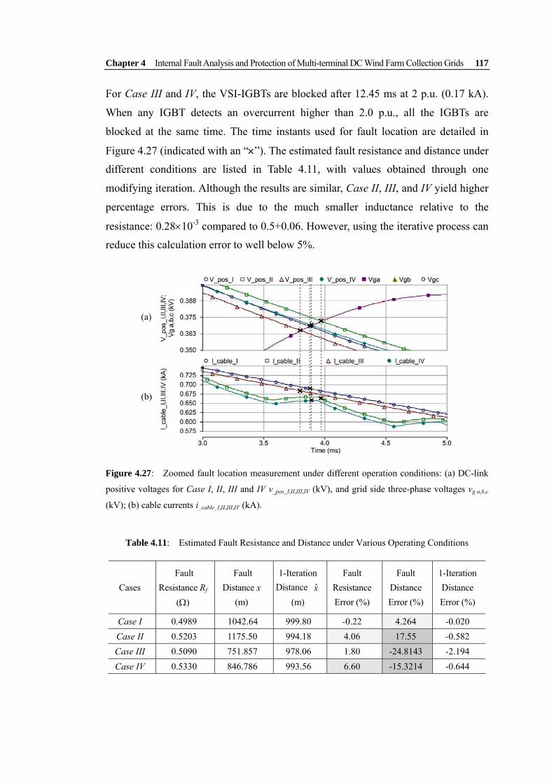
Chapter 4 Internal Fault Analysis and Protection of Multi-terminal DC Wind Farm Collection Grids 117
For Case III and IV, the VSI-IGBTs are blocked after 12.45 ms at 2 p.u. (0.17 kA).
When any IGBT detects an overcurrent higher than 2.0 p.u., all the IGBTs are
blocked at the same time. The time instants used for fault location are detailed in
Figure 4.27 (indicated with an “×”). The estimated fault resistance and distance under
different conditions are listed in Table 4.11, with values obtained through one
modifying iteration. Although the results are similar, Case II, III, and IV yield higher
percentage errors. This is due to the much smaller inductance relative to the
resistance: 0.28×10⁻³ compared to 0.5+0.06. However, using the iterative process can
reduce this calculation error to well below 5%.
Figure 4.27: Zoomed fault location measurement under different operation conditions: (a) DC-link
positive voltages for Case I, II, III and IV v_pos_I,II,III,IV (kV), and grid side three-phase voltages vg a,b,c
(kV); (b) cable currents i_cable_I,II,III,IV (kA).
Table 4.11: Estimated Fault Resistance and Distance under Various Operating Conditions
Cases Fault
Resistance Rf (Ω)
Fault Distance x
(m)
1-Iteration Distance x
(m)
Fault Resistance Error (%)
Fault Distance Error (%)
1-Iteration Distance Error (%)
Case I 0.4989 1042.64 999.80 -0.22 4.264 -0.020 Case II 0.5203 1175.50 994.18 4.06 17.55 -0.582 Case III 0.5090 751.857 978.06 1.80 -24.8143 -2.194 Case IV 0.5330 846.786 993.56 6.60 -15.3214 -0.644
(a)
(b)
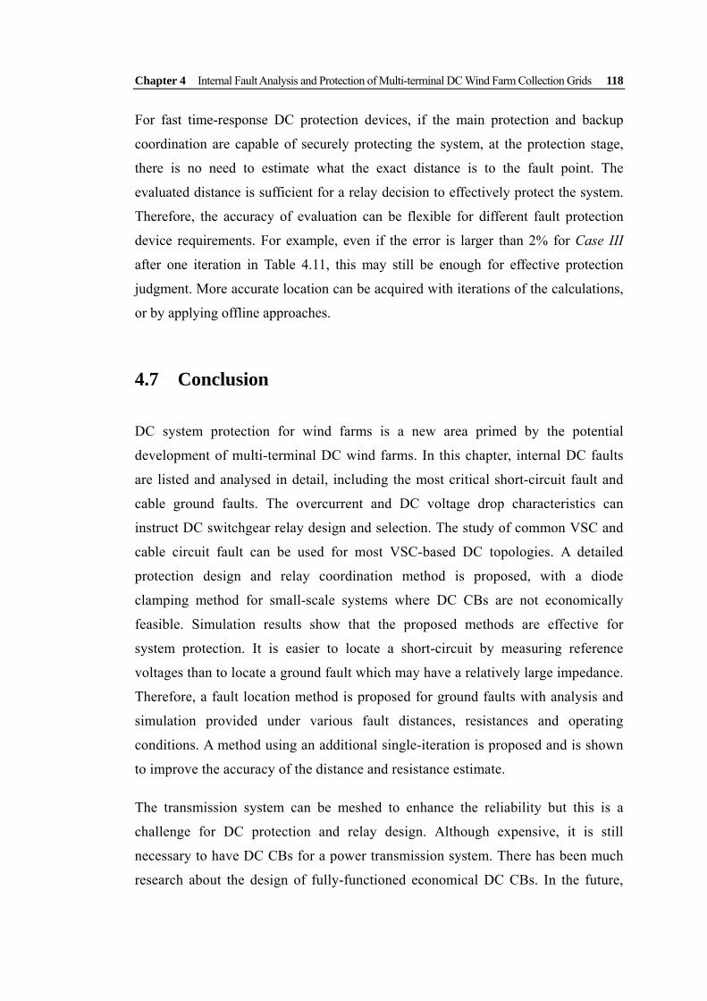
Chapter 4 Internal Fault Analysis and Protection of Multi-terminal DC Wind Farm Collection Grids 118
For fast time-response DC protection devices, if the main protection and backup
coordination are capable of securely protecting the system, at the protection stage,
there is no need to estimate what the exact distance is to the fault point. The
evaluated distance is sufficient for a relay decision to effectively protect the system.
Therefore, the accuracy of evaluation can be flexible for different fault protection
device requirements. For example, even if the error is larger than 2% for Case III
after one iteration in Table 4.11, this may still be enough for effective protection
judgment. More accurate location can be acquired with iterations of the calculations,
or by applying offline approaches.
4.7 Conclusion
DC system protection for wind farms is a new area primed by the potential
development of multi-terminal DC wind farms. In this chapter, internal DC faults
are listed and analysed in detail, including the most critical short-circuit fault and
cable ground faults. The overcurrent and DC voltage drop characteristics can
instruct DC switchgear relay design and selection. The study of common VSC and
cable circuit fault can be used for most VSC-based DC topologies. A detailed
protection design and relay coordination method is proposed, with a diode
clamping method for small-scale systems where DC CBs are not economically
feasible. Simulation results show that the proposed methods are effective for
system protection. It is easier to locate a short-circuit by measuring reference
voltages than to locate a ground fault which may have a relatively large impedance.
Therefore, a fault location method is proposed for ground faults with analysis and
simulation provided under various fault distances, resistances and operating
conditions. A method using an additional single-iteration is proposed and is shown
to improve the accuracy of the distance and resistance estimate.
The transmission system can be meshed to enhance the reliability but this is a
challenge for DC protection and relay design. Although expensive, it is still
necessary to have DC CBs for a power transmission system. There has been much
research about the design of fully-functioned economical DC CBs. In the future,

Chapter 4 Internal Fault Analysis and Protection of Multi-terminal DC Wind Farm Collection Grids 119
this would not be a limitation of DC power system development. The focus of this
chapter has been a radial small-scale DC wind farm, while the conclusions may
extend, suitably modified, to large-scale DC wind farms. The challenges of
protecting meshed large-scale DC wind farm networks will be investigated in
Chapter 5.
Chapter 4 Internal Fault Analysis and Protection of Multi-terminal DC Wind Farm Collection Grids 120
4.8 References
[4.1] P. Bresesti, W. L. Kling, R. L. Hendriks, and R. Vailati, “HVDC connection of offshore wind farms to the transmission system,” IEEE Trans. Energy Convers., vol. 22, no. 1, pp. 37-43, Mar. 2007.
[4.2] C. Meyer, M. Hoing, A. Peterson, and R.W. De Doncker, “Control and design of DC grids for offshore wind farms,” IEEE Trans. Ind. Appl., vol. 43, no. 6, pp. 1475-1482, Nov./Dec. 2007.
[4.3] A. Prasai, J. S. Yim, D. Divan, A. Bendre, and S. K. Sul, “A new architecture for offshore wind farms,” IEEE Trans. Power Electron., vol. 23, no. 3, pp. 1198-1204, May 2008.
[4.4] D. Jovcic and N. Strachan, “Offshore wind farm with centralised power conversion and DC interconnection,” IET Gener. Transm. & Distrib., vol. 3, no. 6, pp. 586-595, Jun. 2009.
[4.5] P. M. Anderson, Power system protection. New York: IEEE Press, 1999.
[4.6] X. Yang, M.-S. Choi, S.-J. Lee, C.-W. Ten, and S.-I. Lim, “Fault location for underground power cable using distributed parameter approach,” IEEE Trans. Power Sys., vol. 23, no. 4, pp. 1809-1816, Nov. 2008.
[4.7] M.-S. Choi, S.-J. Lee, D.-S. Lee, and B.-G Jin, “A new fault location algorithm using direct circuit analysis for distribution systems,” IEEE Trans. Power Del., vol. 19, no. 1, pp. 35-41, Jan. 2004.
[4.8] X. Liu, A. H. Osman, and O. P. Malik, “Hybrid travelling wave/boundary protection for monopolar HVDC line,” IEEE Trans. Power Del., vol. 24, no. 2, pp. 569-578, Apr. 2009.
[4.9] L. Xu, B. R. Andersen, and P. Cartwright, “VSC transmission system operating under unbalanced network conditions – analysis and control design”, IEEE Trans. Power Del, vol. 20, no. 1, pp. 427-434, Jan. 2005.
[4.10] L. Xu, L. Yao, M. Bazargan, and A. Yan, “Fault ride through of large offshore wind farms using HVDC transmission,” in Proc. 2009 IEEE Power Tech Conf., Bucharest, Romania, 28 Jun. – 2 Jul., 2009.
[4.11] M. E. Baran and N. R. Mahajan, “DC distribution for industrial systems: opportunities and challenges,” IEEE Trans. Ind. Appl., vol. 39, no. 6, pp. 1596-1601, Nov./Dec. 2003.
[4.12] M. E. Baran and N. R. Mahajan, “Overcurrent protection on voltage-source-converter-based multiterminal DC distribution systems,” IEEE Trans. Power Del., vol. 22, no. 1, pp. 406-412, Jan. 2007.
[4.13] F. Blaabjerg and J. K. Pederson, “A new low-cost, fully fault-protected PWM-VSI

Chapter 4 Internal Fault Analysis and Protection of Multi-terminal DC Wind Farm Collection Grids 121
inverter with true phase-current information,” IEEE Trans. Power Electron., vol. 12, no. 1, pp. 187-197, Jan. 1997.
[4.14] L. Tang and B. T. Ooi, “Protection of VSC-multi-terminal HVDC against DC faults,” in Proc. IEEE 33rd Annual Power Electronics Specialists Conf., vol. 2, pp. 719-724, Cairns, Queensland, Australia, 23-27 Jun. 2002.
[4.15] L. Tang and B. T. Ooi, “Locating and isolating DC faults in multi-terminal DC systems,” IEEE Trans. Power Del., vol. 22, no. 3, pp. 1877-1884, Jul. 2007.
[4.16] D. Xiang, R. Li, P. J. Tavner, and S. Yang, “Control of a doubly fed induction generator in a wind turbine during grid fault ride-through,” IEEE Trans. Energy Convers., vol. 21, no. 3, pp. 652-662, Sep. 2006.
[4.17] I. Erlich, J. Kretschmann, J. Fortmann, S. Mueller-Engelhardt, and H. Wrede, “Modeling of wind turbines based on doubly-fed induction generators for power system stability studies,” IEEE Trans. Power Syst., vol. 22, no. 3, pp. 909-919, Aug. 2007.
[4.18] M. E. Haque, M. Negnevitsky, and K. M. Muttaqi, “A novel control strategy for a variable speed wind turbine with a permanent magnet synchronous generator,” in Proc. Ind. Appl. Society Annual Meeting, Hobart, Australia, 5-9 Oct. 2008.
[4.19] A. D. Hansen and G. Michalke, “Multi-pole permanent magnet synchronous generator wind turbines’ grid support capability in uninterrupted operation during grid faults,” IET Renewable Power Gener., vol. 3, no. 3, pp. 333-348, Sep. 2009.
[4.20] H. A. Darwish, A.-M. I. Taalab, and M.A. Rahman, “Performance of HVDC converter protection during internal faults,” in Proc. IEEE Power Eng. Society General Meeting, pp. 57-59, Montreal, Quebec, Canada, 18-22 Jun. 2006.
[4.21] M. J. Mousavi and K. L. Butler-Purry, “A novel condition assessment system for underground distribution applications,” IEEE Trans. Power Sys., vol. 24, no. 3, pp. 115-1125, Aug. 2009.
[4.22] S. R. Mendis, M. T. Bishop, J. C. McCall, and W. M. Hurst, “Overcurrent protection of capacitors applied on industrial distribution systems,” IEEE Trans Ind. Appl., vol. 29, no. 3, pp. 541-547, May/Jun. 1993.
[4.23] K. Xing, F. C. Lee, J. S. Lai, T. Gurjit, and D. Borojevic, “Adjustable speed drive neutral voltage shift and grounding issues in a DC distribution system,” in Proc. IEEE Ind. Appl. Society Annual Meeting, New Orleans, Louisiana, 5-9 Oct. 1997.
[4.24] C. Abbey, W. Li, L. Owatta, and G. Joós, “Power electronic converter control techniques for improved low voltage ride through performance in WTGs,” in Proc. 37th IEEE Power Electronics Specialists Conference, vol. 1, pp. 422-427, Jeju, Korea, 18-22 Jun. 2006.
[4.25] S. Castagno, R. D. Curry, and E. Loree, “Analysis and comparison of a fast turn-on series IGBT stack and high-voltage-rated commercial IGBTs,” IEEE Trans. Plasma Science, vol. 34, no. 5, pp 1692-1696, Oct. 2006.

122
Chapter 5 Protection Coordination of Meshed VSC-HVDC Transmission Systems for Large-Scale Wind Farms
5.1 Introduction
The Supergrid is a conceptual and ambitious European development to assist the
integration of renewables and European connectivity [5.1], [5.2]. It is a high-voltage
meshed DC grid that connects together a number of wind farms and onshore
substations in participating European countries. High-voltage direct-current (HVDC)
technology based on voltage-source converters (VSCs) is a flexible technology that
could realise the Supergrid concept even with some weak AC system connections
[5.3]. The meshed topology aims to enhance system reliability, which is requisite for
transmission networks with a large contribution from offshore wind power. Networks
with loops are common in traditional AC transmission power grids, because they are
relatively economical compared to the double-line systems and more reliable than
radial systems without backup. The potentially large capacity of wind power
integrated into AC grids requires the transmission systems to be much more reliable
due to its influence on the whole electricity system. If the concept of Supergrid
progresses to reality for multiple wind farm connection and integration to onshore
systems, issues related to the loop topology should be considered in advance,
especially for the untried high-power DC scenario.
Due to the lack of existing high-power DC systems and associated operational
experience, currently there is no developed protection scheme that can be used for
the VSC-based high-power DC scenario. In order to help solve the DC system

Chapter 5 Protection Coordination of Meshed VSC-HVDC Transmission Systems for Large-Scale Wind Farms 123
protection problem, radial multi-terminal DC VSC-based overcurrent protection for
wind power generation is discussed in Chapter 4, which will form the basis of this
chapter. As mentioned, there is little work on VSC-based DC system switchgear
configuration for protection. However, for large-scale offshore DC wind farms with
HVDC power transmission, proper DC switchgear configuration is essential.
Therefore, this chapter will further explore the protection design of meshed networks
at the transmission level. Former fault analysis of VSC-cable systems will be
summarised and applied. The DC switchgear technology is assumed to be a
uni-directional current-blocking power electronic circuit breaker (CB). The key
protection issues to realise protection reliability and selection of this meshed DC
network are defined and discussed with a consequent CB tripping strategy.
This chapter is organised as follows. In Section 5.2, the multi-terminal DC wind farm
topology is introduced along with possible topologies. A typical network section is
proposed for study. DC fault characteristics are summarised and applied in Section
5.3. With fault current frequency analysis, the DC cable modelling issue is discussed
with comparisons via simulation. DC switchgear options and their allocation are
presented in Section 5.4 followed by detailed protection strategy design. Illustrative
examples and PSCAD/EMTDC simulations are provided in Section 5.5.
5.2 Multi-terminal Meshed DC Wind Farm Network
Nowadays, multi-terminal DC wind farm topologies that have been researched are
mainly radial [5.4], [5.5]. However, a meshed connection is required for future
reliable HVDC power transmission [5.2]. There is currently no reported work about
the protection of such systems.
5.2.1 Meshed Multi-terminal DC Wind Farm Topology
The topology with loops is commonly used in traditional AC power transmission
systems because of its balance between economic costs and reliability. The
high-power DC transmission network will need to achieve the highest standard of
reliability and availability. If the concept of Supergrid can be realised for multiple

Chapter 5 Protection Coordination of Meshed VSC-HVDC Transmission Systems for Large-Scale Wind Farms 124
offshore wind farm connection and integration to different onshore AC grids, the
protection issues related to the meshed system must be addressed. For the collection
grid, the reliability can also be enhanced by introducing redundant cables (discussed
in Chapter 6), but usually, the system will operate in open-loop which leaves all the
redundant cables as backup in case of faults in cables or devices used during normal
operation. If many wind farms are connected together with multiple onshore
connections, the transmission system should be optimal to have a loop, or even
meshed. Power flows in this network can be much more flexible with a more even
utilisation of cable resources, which is one of the most expensive investments.
However, this meshed topology makes the protection relay coordination and
switchgear system much more complex.
One main problem for a complex loop/meshed system is that the power flow cannot
be predicted accurately. The power flow varies as the system condition changes, for
example, wind speed oscillations that result in power fluctuations, or possible power
flow direction changes due to switch-in or -out of wind farms. Special attention to
the loop cables between wind farms is required because of the bi-directional load
flow on them. Therefore the possible normal power flow oscillations and direction
changes need to be excluded to make the relay setting simpler and accurate in
operation. Apart from that, mature protection and relay coordination techniques of
meshed AC distribution and transmission systems [5.6]-[5.8] can be analysed and
developed for application to this DC system.
5.2.2 Supergrid Section for Protection Test Study
The DC topology investigated is a multi-terminal VSC-HVDC system connecting
large-scale wind farms. A typical section of this meshed DC Supergrid with possible
switchgear allocation for protection test is shown in Figure 5.1. All the AC/DC
rectifiers and DC/AC inverters are sinusoidal pulse-width-modulation (SPWM)
VSCs connected with DC cables (lengths as shown). No more detailed DC wind
farm collection grids are shown, only the transmission system with converters or
centralised step-up DC/DC converters illustrated as VSCs. Each wind farm is
represented by an equivalent wind turbine-permanent magnet synchronous generator

Chapter 5 Protection Coordination of Meshed VSC-HVDC Transmission Systems for Large-Scale Wind Farms 125
(PMSG) set in which maximum-power-point-tracking (MPPT) is fulfilled by the
AC/DC VSC. The rectifier VSC and voltage source inverter (VSI) control schemes
are that of a single PMSG direct-driven wind power generation system [5.9]. The
four wind farms are all of 300 MW rating each – 1200 MW in total – and connected
to a ±100kV DC loop with two parallel cables to two separate onshore AC grids.
AC Grid 1
Wind Farm 1
AC Grid 2
VSI2
Wind Farm 2 DC Cables
VSC
Wind Farm 3
VSC
Wind Farm 4
VSI1
VSC
VSC
Circuit Breaker / Switchgear and its Relay System
f1 f2
(300 MW)
(300 MW)
(300 MW)
(300 MW)
(+100 kV)
(−100 kV)
(200 km) (200 km)
(200 km) (200 km)
(200 km) (200 km)
(+100 kV)
(−100 kV)
(60 km)
f3
(60 km)
Figure 5.1: A typical section of multi-terminal DC transmission system for Supergrid.
This example transmission section is made according to the following assumptions: 1)
Each node has a connection to a wind farm or onshore inverter platform to AC grid
substation; 2) The loop here is symmetrical with connections to two AC grids; 3)
There might not be real DC bus conductors allocated in an offshore environment, but
the node with more than two connections is considered to be a DC bus where bus
faults can occur (shown as fault f2 in Figure 5.1).
This network is simplified to a single-line diagram, Figure 5.2, for node/cable
numbering and possible power flow directions indicated with dotted arrows. The
Cables 1, 3, 4 and 5 are defined as loop cables; while Cables 2 and 6 are radial cables.
It is the bi-directional loop Cables 1, 3, 4, 5 that complicate the protection
coordination.

Chapter 5 Protection Coordination of Meshed VSC-HVDC Transmission Systems for Large-Scale Wind Farms 126
(1) (3) (5)
(2) (4) (6)
Cable 1
Wind Farm 3 Pwf3
Wind Farm 1 Pwf1
AC Grid 1
AC Grid 2
Pwf4 Wind Farm 4
Pwf2 Wind Farm 2
Cable 2
Cable 5 Cable 6
Cable 3 Cable 4
Figure 5.2: Single-line diagram shows system nodes, cable connections, and power flow directions.
IGBT-based VSCs have freewheel diodes − as shown in Figure 5.3(b) − which will
be destroyed by the overcurrent that occurs during DC-link discharge. Fault tolerant
converters can be applied to avoid allocating a large number of DC CBs. The main
idea is to replace those passive diodes with self turn-off power electronic devices,
like another IGBT/diode series branch (Figure 5.3(c)) or emitter turn-off devices
(ETOs) [5.10] (Figure 5.3(d)). Furthermore, a thyristor-based dedicated high-power
DC/DC transformer that can isolate fault currents is proposed in [5.11]. However, in
terms of a network, this means all the converters need to be totally immune from DC
faults. During the development of the network, at this stage, with mostly
conventional VSCs, it is economically infeasible. Therefore, protection scheme
design is still a necessity to the development of multi-terminal DC transmission
networks.
IGBT
Freewheel Diode
ETO
(a) (b) (c) (d)
Figure 5.3: Illustration of VSC switch configuration for fault tolerant function: (a) switch symbol;
(b) traditional IGBT/diode switch; (c) bi-directional IGBT/diode-series fault tolerant switch; (d)
bi-directional IGBT/ETO parallel fault tolerant switch.
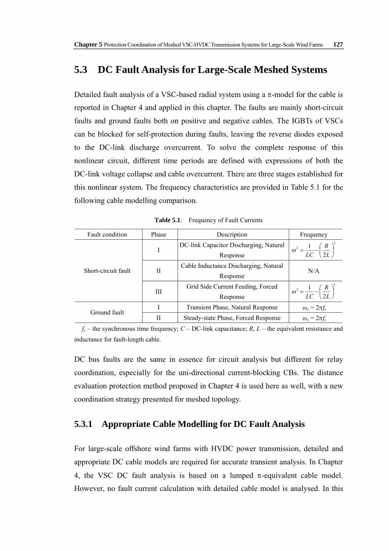
Chapter 5 Protection Coordination of Meshed VSC-HVDC Transmission Systems for Large-Scale Wind Farms 127
5.3 DC Fault Analysis for Large-Scale Meshed Systems
Detailed fault analysis of a VSC-based radial system using a π-model for the cable is
reported in Chapter 4 and applied in this chapter. The faults are mainly short-circuit
faults and ground faults both on positive and negative cables. The IGBTs of VSCs
can be blocked for self-protection during faults, leaving the reverse diodes exposed
to the DC-link discharge overcurrent. To solve the complete response of this
nonlinear circuit, different time periods are defined with expressions of both the
DC-link voltage collapse and cable overcurrent. There are three stages established for
this nonlinear system. The frequency characteristics are provided in Table 5.1 for the
following cable modelling comparison.
Table 5.1: Frequency of Fault Currents
Fault condition Phase Description Frequency
I DC-link Capacitor Discharging, Natural
Response
22
21
⎟⎠⎞
⎜⎝⎛−=
LR
LCω
II Cable Inductance Discharging, Natural
Response N/A Short-circuit fault
III Grid Side Current Feeding, Forced
Response
22
21
⎟⎠⎞
⎜⎝⎛−=
LR
LCω
I Transient Phase, Natural Response ωs = 2πfs Ground fault II Steady-state Phase, Forced Response ωs = 2πfs
fs – the synchronous time frequency; C – DC-link capacitance; R, L – the equivalent resistance and inductance for fault-length cable.
DC bus faults are the same in essence for circuit analysis but different for relay
coordination, especially for the uni-directional current-blocking CBs. The distance
evaluation protection method proposed in Chapter 4 is used here as well, with a new
coordination strategy presented for meshed topology.
5.3.1 Appropriate Cable Modelling for DC Fault Analysis
For large-scale offshore wind farms with HVDC power transmission, detailed and
appropriate DC cable models are required for accurate transient analysis. In Chapter
4, the VSC DC fault analysis is based on a lumped π-equivalent cable model.
However, no fault current calculation with detailed cable model is analysed. In this
Chapter 5 Protection Coordination of Meshed VSC-HVDC Transmission Systems for Large-Scale Wind Farms 128
section, the multi-layered underground (or submarine) distributed cables are analysed
because they are used in practice for large-scale onshore/offshore wind power
integration. Overhead line models are not investigated.
1) Existing Cable Models
There are several cable models available for circuit analysis and computer simulation.
Theoretically, the distributed single-conductor cable model is represented by partial
derivative equations in time and distance as the original mathematical model.
Furthermore, to separate distance and time dependency, the travelling wave model
analysis [5.12] is performed for steady-state solution under ideal sinusoidal signals.
For transient response simulations, there are four common models. The most
common, and simple, is the π-equivalent model. The Bergeron model is a
progression of the simple π-model. It accurately represents the distributed L and C,
but with a lumped R to simulate cable power loss. They are accurate at a specified
frequency and are suitable for studies where a certain frequency is important (e.g.,
for AC relay studies) [5.13]. The frequency dependent model in mode represents the
frequency dependence of all parameters (not just at the specified frequency as in the
Bergeron model). The problem of a frequency dependent transformation matrix can
be overcome by formulating the model directly in the phase domain (without
diagonalisation) [5.13], which results in the frequency dependent phase model. It
also represents the frequency dependence of all parameters as in the mode model,
and produces the most accurate transient responses.
Therefore, the choice of cable model mainly depends on the frequency range of the study.
Appropriate cable models will be chosen for the DC fault protection analysis with
simulation comparison as verification of the former π-model analysis in Chapter 4.
2) Fault Current Frequency
Traditional fault analysis and solutions for AC distribution and transmission systems
are well understood and have led to mature technologies. To clarify the analysis for
traditional AC system fault conditions, the capacitor discharging part in the AC fault
analysis is introduced here as a reference.
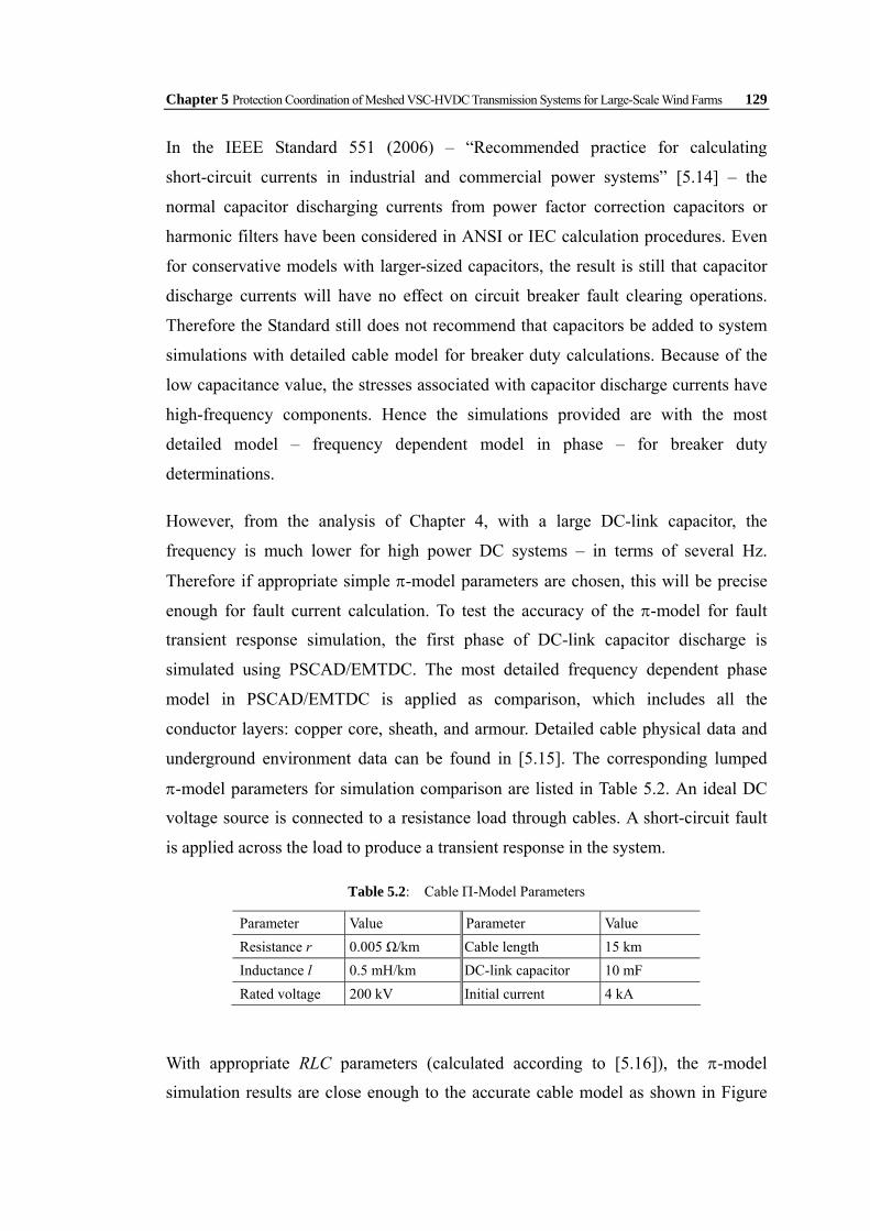
Chapter 5 Protection Coordination of Meshed VSC-HVDC Transmission Systems for Large-Scale Wind Farms 129
In the IEEE Standard 551 (2006) – “Recommended practice for calculating
short-circuit currents in industrial and commercial power systems” [5.14] – the
normal capacitor discharging currents from power factor correction capacitors or
harmonic filters have been considered in ANSI or IEC calculation procedures. Even
for conservative models with larger-sized capacitors, the result is still that capacitor
discharge currents will have no effect on circuit breaker fault clearing operations.
Therefore the Standard still does not recommend that capacitors be added to system
simulations with detailed cable model for breaker duty calculations. Because of the
low capacitance value, the stresses associated with capacitor discharge currents have
high-frequency components. Hence the simulations provided are with the most
detailed model – frequency dependent model in phase – for breaker duty
determinations.
However, from the analysis of Chapter 4, with a large DC-link capacitor, the
frequency is much lower for high power DC systems – in terms of several Hz.
Therefore if appropriate simple π-model parameters are chosen, this will be precise
enough for fault current calculation. To test the accuracy of the π-model for fault
transient response simulation, the first phase of DC-link capacitor discharge is
simulated using PSCAD/EMTDC. The most detailed frequency dependent phase
model in PSCAD/EMTDC is applied as comparison, which includes all the
conductor layers: copper core, sheath, and armour. Detailed cable physical data and
underground environment data can be found in [5.15]. The corresponding lumped
π-model parameters for simulation comparison are listed in Table 5.2. An ideal DC
voltage source is connected to a resistance load through cables. A short-circuit fault
is applied across the load to produce a transient response in the system.
Table 5.2: Cable Π-Model Parameters
Parameter Value Parameter Value Resistance r 0.005 Ω/km Cable length 15 km Inductance l 0.5 mH/km DC-link capacitor 10 mF Rated voltage 200 kV Initial current 4 kA
With appropriate RLC parameters (calculated according to [5.16]), the π-model
simulation results are close enough to the accurate cable model as shown in Figure
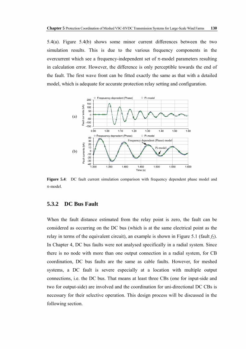
Chapter 5 Protection Coordination of Meshed VSC-HVDC Transmission Systems for Large-Scale Wind Farms 130
5.4(a). Figure 5.4(b) shows some minor current differences between the two
simulation results. This is due to the various frequency components in the
overcurrent which see a frequency-independent set of π-model parameters resulting
in calculation error. However, the difference is only perceptible towards the end of
the fault. The first wave front can be fitted exactly the same as that with a detailed
model, which is adequate for accurate protection relay setting and configuration.
Frequency dependent (Phase) model
Pi-model
Figure 5.4: DC fault current simulation comparison with frequency dependent phase model and
π-model.
5.3.2 DC Bus Fault
When the fault distance estimated from the relay point is zero, the fault can be
considered as occurring on the DC bus (which is at the same electrical point as the
relay in terms of the equivalent circuit), an example is shown in Figure 5.1 (fault f2).
In Chapter 4, DC bus faults were not analysed specifically in a radial system. Since
there is no node with more than one output connection in a radial system, for CB
coordination, DC bus faults are the same as cable faults. However, for meshed
systems, a DC fault is severe especially at a location with multiple output
connections, i.e. the DC bus. That means at least three CBs (one for input-side and
two for output-side) are involved and the coordination for uni-directional DC CBs is
necessary for their selective operation. This design process will be discussed in the
following section.
(a)
(b)

Chapter 5 Protection Coordination of Meshed VSC-HVDC Transmission Systems for Large-Scale Wind Farms 131
5.4 Protection Scheme for Meshed DC Systems
According to the analysis in Section 5.3, the protection scheme design depends on
the fault characteristics and the type of CB applied. The key issue is the strategy of a
selective but reliable CB coordination method. The proposed protection coordination
is realised by distance evaluation without communication between distant relays. The
CB fault tripping requirements are: 1) The DC current and voltage are required to be
continuously monitored during system operation. 2) When overcurrent is detected, the
equivalent fault distance is evaluated rapidly using a voltage difference comparison
method. 3) The assessed distance will be used to compare with the relay pre-set values
to decide when and whether to trip the CB or not.
5.4.1 High-Power DC Switchgear Allocation
High-power DC switchgear is still under development with few mature commercial
products. The traditional mechanical structured CB used in AC systems cannot be
applied due to the slow fault isolation speed and the requirement of zero-crossings in
the fault current. Therefore, power electronic devices are used to quickly block fault
currents, such as IGBT and gate turn-off thyristors (GTOs). Generally, CBs of this
kind are called solid-state CBs (SSCBs). One option includes a paralleled mechanical
switch Sp as an auxiliary switch for lower loss during normal operation, a
metal-oxide-varistor surge arrester MOVCB, and power electronic blocking device
PECB, Figure 5.5(a). The PECB block can be a parallel or series topology. Figure 5.5(b)
and 5.5(c) realise bi-directional current block functions. Sometimes, a series
inductance LCB and a switch Ss are used as a fault current limiter and to provide an
obvious electrical isolation point for the network operator, i.e. as a disconnector. This
CB topology can be seen as device redundancy to enhance reliability, as a
comparison with topology redundancy which will be discussed in Chapter 6.
The technical challenges for high-power DC CBs are the current isolation capability
of power electronic devices, their high costs and their losses. Although some fault
tolerant converters can reduce the allocation of CBs, as long as the development of
this DC network includes traditional VSCs, reliable system protection relies on DC

Chapter 5 Protection Coordination of Meshed VSC-HVDC Transmission Systems for Large-Scale Wind Farms 132
CBs. At this stage, in terms of device number, it is still economical to allocate DC
CBs. Multi-IGBT devices could be used in series or parallel connection to increase
the voltage or current ratings, particularly for high-overcurrent situations.
The DC switchgear allocation is illustrated in Figure 5.6 for the six-node test system.
Uni-directional current-blocking DC CBs are used. This is a trade-off option
considering both economic costs and function. The CB at each cable end has only
one IGBT for fault current blocking but the two CBs can cooperate to isolate faults
that occur between them on the cable. This requires only half the number of power
electronic devices for fault current cut-off compared to the fully functioned
bi-directional CBs, with half the loss but with a reduction in functionality. This CB
allocation and configuration will influence the coordination strategy design. If
bi-directional functionalised CBs are used, the multi-loop coordination strategy of
the AC system can be applied to this DC loop protection analysis [5.6], [5.7].
LCB PECB
Sp Ss
MOVCB
CB
Parallel PECB
Series PECB
(a) (b) (c)
Figure 5.5: A DC CB option: (a) DC CB configuration; (b) parallel connected bi-directional PE
block; (c) series connected bi-directional PE block.
(1) (3) (5)
(2) (4) (6)
[1] [2]
[3] [4] [5] [6] [7] [8]
[9] [10] [11] [12] [13] [14]
[15] [16]
Wind Farm 3 Wind Farm 1
to AC Grid 1
to AC Grid 2
Wind Farm 4 Wind Farm 2
(*) Node number [*] CB number
f1
f2
f3
Figure 5.6: DC CB allocation and numbering for relay configuration and coordination.

Chapter 5 Protection Coordination of Meshed VSC-HVDC Transmission Systems for Large-Scale Wind Farms 133
The operating state of the wind farm depends on the wind resource conditions. The
power acquired from a large wind turbine is variable but normally varies over at time
period of seconds. Simulation of variable wind speed conditions have been
performed using the wind profile shown in Figure 5.7. In the simulation, the whole
wind farm is exposed simultaneously to the wind profile which is the most severe
case of power flow and current variation on the cable. The wind model applied is
from PSCAD/EMTDC with gusts, noise and a rated speed of 12 ms−1. The shear and
tower effects which result in a flicker power quality problem [5.17] are not
considered. This will not influence the protection system operation.
The results in Figure 5.7 show that: 1) There can be steep current increase and
decrease; 2) DC-link voltage fluctuation is not as dramatic as under fault conditions.
With many distributed wind-turbines aggregation reduces the fluctuation effect.
Hence the power fluctuation due to changes in wind conditions will not influence the
relay system performance as long as the rate of change of current is not utilised for
fault detection. The DC fault currents are always extreme where overcurrent occurs
in milliseconds and is distinct enough from normal fluctuations for fault
identification.
Figure 5.7: DC cable current and voltage responses under wind speed fluctuation: (a) wind speed
(ms−1); (b) cable current (p.u.); (c) inverter DC-link voltage (p.u.).
(a)
(b)
(c)

Chapter 5 Protection Coordination of Meshed VSC-HVDC Transmission Systems for Large-Scale Wind Farms 134
Figure 5.8: DC cable current and voltage responses under sudden power increase: (a) cable currents
(p.u.); (b) inverter DC-link voltage (p.u.).
The power flow calculation for this linear system will obey basic physical principles,
which will not need a specific algorithm for the convergence of results, like those
commonly used for nonlinear AC systems. In this DC system, all the power sources
can be calculated separately to estimate current flow according to the superposition
theorem. Therefore the theoretical power flow results can be calculated almost
instantaneously which is helpful for the real-time decision process. Figure 5.8 shows
a power increase due to a change in system operation. There are high rates of change
of current in some cables which reinforces the need to not use rate of change of
current in the decision making process.
Another issue is the exclusion of current harmonics due to the modulation method of
the converters [5.15]. The harmonics are with known high-order frequencies and can
be eliminated from the method used to detect faults via frequency detection. Hence,
only in the low frequencies given in Table 5.1, current and DC-link voltage
amplitude and direction changes will the signals be used to detect fault conditions.
5.4.2 DC CB Relay Coordination Relations
For a very complex multi-loop network, it is necessary to describe the relay
coordination relations by definition of the dependency degrees [5.7], [5.8]. The
primary protection relay set (PPRS), primary protection dependency degree (PD) and
backup protection dependency degree (BD) are defined as functional dependency
[5.7].
(a)
(b)

Chapter 5 Protection Coordination of Meshed VSC-HVDC Transmission Systems for Large-Scale Wind Farms 135
Protection setting of relay R[x] depends on the relay setting R[i], R[j], …, R[n] to realise
coordination. Then R[i], R[j], …, R[n] is called the PPRS. Number n is defined as PD.
According to the cooperation principle between primary protective relays and backup
protective relays, the protection relay R[2] should cooperate with R[1], i.e., the setting
value of R[2] must be calculated in terms of the setting value of R[1]. Moreover, the
time delay of the backup R[2] must avoid the most serious diode freewheel phase
(short-circuit fault phase II in Table 5.1). Analogically, R[3] cooperates with R[2], R[m]
cooperates with R[m–1], and R[1] cooperates with R[m] as a loop. Consequently, the
cooperation relations among protective relays R[1], R[2], …, R[m–1], R[m] result in a
circulation. BD is the number of this relay which can act as backup for others. Table
5.3 shows the PPRS, PD and BD of all the relays in the example section network in
Figure 5.6.
Table 5.3: Relay Coordination Relations and Coordination Dependency Degrees
Relay PPRS PD BD Relay PPRS PD BD [1] ∅ 0 2 [9] [1], [4] 2 1 [2] ∅ 0 3 [10] [12], [13], [16] 3 1 [3] [10], [15] 2 1 [11] [9], [15] 2 2 [4] [2], [6], [7] 3 1 [12] [2], [5], [7] 3 2 [5] [1], [3] 2 2 [13] AC Grid 2 1 2 [6] [11], [13], [16] 3 2 [14] [11], [12], [16] 3 0 [7] AC Grid 1 1 2 [15] ∅ 0 2 [8] [2], [5], [6] 3 0 [16] ∅ 0 3
These dependency degrees are used to determine the Minimum loop-Breaking Point
Set (MBPS) for multi-loop systems to be broken down to radial systems, then the
simple distance coordination method can be carried out to realise selection. If
DC/DC isolation transformers are applied [5.11], the system can be automatically
separated into radial sub-networks. But this requires reliable DC/DC transformers
and additional device costs and power losses will be incurred.
5.4.3 Protection Scheme
The steps of the protection scheme are defined as follows and are illustrated in
Figure 5.9.

Chapter 5 Protection Coordination of Meshed VSC-HVDC Transmission Systems for Large-Scale Wind Farms 136
1) Relay setting preparation• Overcurrent threshold ith (2.1 p.u.) • Voltage drop threshold vth (0.5 p.u.)
2) Normal operation monitoring:Relay point current and voltage
measurements
3) DC fault detection vrelay vth
&
irelay ith
4) Fault distance x evaluation
• Calculate critical fault clearing time tc
• Radial cable x=0 • Loop cable x<D • Bus cable x=D …
6) Tripping decision: Protective selection without
relay communication
True
7) CB tripping operation
tdelay
>
<
• Short-circuit fault distance • Ground fault distance &
grounding resistance
tdec
tCB
tmea
5) MBPS determination • Radial sub-systems
Figure 5.9: The proposed DC meshed network protection scheme.
1) Relay setting preparation: At the planning stage, the overcurrent threshold ith and
voltage drop threshold vth are set. In this section, ith is chosen as 2.1 p.u. to avoid
tripping during normal operation when power flow could be 2.1 p.u. due to a
previous CB trip (assume normal operation can be up to 1.05 p.u. for each wind
farm). The voltage drop threshold is vth = 0.5 p.u. for the DC-link voltage.
2) Real-time monitoring: For each wind resource sampling period (e.g. one second),
calculate the system power flows and measure relay point current and voltage
amplitudes for each sampling period (e.g. 50 μs) as state monitoring. The
measurement equipment should have a small sampling time period to ensure the
relays have enough sampling points to deal with fault detection and tripping
operation.
3) Real-time fault detection: The abrupt change of currents and DC-link voltage
collapse are compared with the pre-set threshold values. Practically, this will take
at least one current and voltage sampling time-step to complete.

Chapter 5 Protection Coordination of Meshed VSC-HVDC Transmission Systems for Large-Scale Wind Farms 137
4) Real-time distance evaluation: After the fault is detected, the distance calculation
is performed using voltage comparison. As proposed in Chapter 4, a reference
relay voltage sensor unit (ri) is equipped for the relative voltage calculation; it is
located near the main relay point on the same section of cable, as shown in Figure
5.10, to avoid long distance communication issues. Voltage dividers are used for
voltage measurements. The distance between them is known as d, so the fault
distance measured from this reference is
( ))()()( nrnn vvvdx −= . (5.1)
x
(flt) (n) d
(rn) i(n) i(flt)
(m) (rm) d
Figure 5.10: Distance evaluation with two voltage divider measurements.
5) Real-time MBPS determination: The multi-loop breaking-points are chosen with
the BD relation of the minimum distance relay points as the start. Then the
system is separated into radial branches with the MBPS.
6) Tripping decision: If a fault is detected from step 3), a corresponding relay delay
time for the CB will be applied. At this stage a decision is made as to whether the
fault is in the protection region of this CB. It will trip after a given delay time as
backup protection, or immediately as primary protection. Firstly, the critical time
tc (for short-circuit fault phase II in Table 5.1) is calculated at each relay point as
the tripping period upper limit, as proposed in Chapter 4. In respect of the
evaluated distance x, the critical time is
( )ω
δωπ′
−′−=
)(arctan 000 ICVCVtc (5.2)
where 220 δωω −=′ x , 22
0 ωδω += , δ = R/(2L), ω2 = 1/(LC) − [R/(2L)]2. C,
R, and L are the DC-link capacitance, fault-length DC cable equivalent π-model
resistance and inductance respectively. The values of V0 and I0 used are from
real-time measurement one time-step before the fault detection. This critical time
tc will be used to set the upper limit of relay delay time for backup CBs.

Chapter 5 Protection Coordination of Meshed VSC-HVDC Transmission Systems for Large-Scale Wind Farms 138
7) CB tripping operation: After waiting for the consequent time delay, the CB trips
with IGBT block and possible disconnector operation. The total operation time
until the fault current is finally extinguished is designated as tCB.
The total protection clearing time includes the measurement time tmea, decision and
evaluation time tdec, resulting delay time tdelay, and CB time tCB, as shown in Figure 5.9.
Again this has to be finished before the appropriate critical time tc. The selection decision
step without relay communication is described in detail as follows.
5.4.4 Protective Selection without Relay Communication
To avoid the use of communication between distant relays, the selection is realised
by the following assumptions and measurement allocations.
1) The CBs just connected to one radial cable or a wind farm will operate
immediately only when their evaluated distance x is exactly or almost zero. The
DC-chopper system across the wind farm DC-link needs to operate to dump all
the redundant power. Meanwhile the wind farm needs to be stopped. If x is not
zero, it will always wait for a delay time for the primary cable protection to
operate and form a possible new power transmission route in the loop.
2) If the CB at one end of the cable detects exactly the cable length D as fault
distance, this means the fault has occurred at the DC bus connected to other end of
this cable. This CB will trip immediately because the CB near the DC bus cannot
block fault current by itself due to the reverse diode of the CB in which reverse
current flows. This is the main difference from AC protection, where the CB near
an AC bus is the fastest primary protection. However, this depends on the
accuracy of distance evaluation algorithm, especially for a ground fault with
grounding resistance. Hence an accurate and efficient fault distance evaluation
method is required.
3) If the evaluated distance value is negative, that means the fault did not occur on
this cable, so it will wait for a delay time (as shown the CB relay point (m) in

Chapter 5 Protection Coordination of Meshed VSC-HVDC Transmission Systems for Large-Scale Wind Farms 139
Figure 5.10, for the fault (flt), v(m) < )( mrv , hence evaluated distance
( ) 0)()()( <−=mrmm vvvdx ).
Three typical fault condition coordination decision examples are shown in detail in
Table 5.4 to better describe the decision process. 1) For loop cable fault f3 in Figure
5.1, firstly the evaluated absolute distance range is used to classify all the relay
points, where D is the cable length (e.g. 200 km in Figure 5.1). 2) Then for each
category, the “+” distance relays are the primary protections because the fault is
detected within its protection range. For others in this category, those only connected
to a VSC source are in the second order, because if the primary protection CBs fail to
trip, it can be seen as a bus fault, where the VSC definitely needs to be tripped. 3)
The others in this category are ranked as the third order.
The ordering is carried on until all the categories are sorted to reach a tripping order
result. These rules are the same as for a radial cable fault like f1. However, for DC
bus fault, it is different, as stated the CB near the faulted DC bus cannot isolate fault
current flows through reverse diodes. Therefore if a relay evaluated distance is
exactly the cable length D, its CB has the priority to trip primarily, e.g. relay R[4], R[8],
and R[12] in Table 5.4 under bus fault f2.
Communication may be needed for CB relays at the same DC bus but because they are
physically close communication is practical. A cable ground fault with a large
resistance is not as serious as a short-circuit fault and some time delay is permitted.
But a ground fault on the DC bus can be precisely detected even without accurate
grounding resistance evaluation. For example, it is easy for relay R[2] to identify a bus
fault when the ground distance evaluation is exactly the same with R[5], R[6], and R[7].
The cable length inductance ratio with typical grounding resistance can be used as a
reference for a fuzzy decision. For instance, evaluated distance from R[4] may not be
exactly D, but 1.5D. However, it still needs to trip first as the primary protection. A
more accurate and faster DC ground fault location and resistance assessment has been
proposed in Chapter 4.

Chapter 5 Protection Coordination of Meshed VSC-HVDC Transmission Systems for Large-Scale Wind Farms 140
Table 5.4: Protective O
rder Selection without R
elay Com
munication

Chapter 5 Protection Coordination of Meshed VSC-HVDC Transmission Systems for Large-Scale Wind Farms 141
5.5 DC Wind Farm Protection Simulation Results
A simulation system of the proposed Supergrid section is modelled in
PSCAD/EMTDC. Network parameters of the system are shown in Figure 5.1. The
PMSG and VSC parameters are provided in Tables 5.5 and 5.6. A detailed frequency
dependent phase cable model is employed in the simulations. The same DC cable
π-model parameters in Table 5.2 are used for critical tripping time tc calculations. The
proposed protection scheme is applied to this specific DC wind farm system to show
the protection results. The faults simulated are short-circuit faults and ground faults at
the three selected points in Figure 5.1 and Table 5.4. After the faults occur, the VSC
IGBTs are blocked for self-protection. The per unit power calculation uses 600 MW as
base value for each grid-side VSI connected to an AC grid. Finally in Section 5.5.4, the
aforementioned cable modelling comparison is also performed on this system for a
short-circuit fault.
Table 5.5: PMSG Parameters
Parameter Value Parameter Value Rated power Pn 300 MW Pole pair no. Pp 100 Rated stator voltage Vsn 99 kV Phase resistance 0.068 p.u. Rated frequency fg 50 Hz Phase inductance 0.427 p.u.
Table 5.6: VSC Parameters
Value Parameter
Wind Farm VSC Rectifier AC Grid VSC Inverter Rating Power 300 MW 600 MW DC Voltage ±100 kV ±100 kV DC-link capacitance 10 mF 20 mF Choke inductance 18 mH 22 mH Transformer voltages 99 kV / 96 kV 96 kV / 110 kV
5.5.1 DC Radial Cable Short-Circuit/Ground Fault Condition
A short-circuit and a positive-side metallic ground fault are applied at f1 (60 km from
the VSI1) at t = 10.0s, respectively. Figures 5.11 and 5.12 are the fault overcurrents

Chapter 5 Protection Coordination of Meshed VSC-HVDC Transmission Systems for Large-Scale Wind Farms 142
without protection. In Figure 5.11, the total short-circuit fault current for VSI1 side
i(fault) reaches more than 210 kA – up to 70 times of the rated value (3.0 kA for 600
MW wind power transmitted in ±100 kV voltage level). The main contribution
comes from the discharge of the large DC-link capacitor. After the capacitor
discharge phase, the most vulnerable component - diodes - suffer during the
freewheel phase (short-circuit phase II in Table 5.1). The diode freewheel overcurrent
phase happens after 28 milliseconds, with abrupt VSI current i(VSI) distributed in the
three phase diodes D1, D3, and D5 as i(D1), i(D3), and i(D5). This abrupt overcurrent is
about 5 times normal (from 15 kA to 75 kA). This has the most serious impact on the
VSC-HVDC system and will immediately destroy the converter. At the same time,
the AC-side grid currents will feed into the fault point through VSI1 diodes, which
results in the oscillation and absorption of active and reactive power from the AC
grids (shown in Figure 5.13).
i(fault)
i(C) i(VSI)
i(D1), i(D3), i(D5)
Figure 5.11: Short-circuit fault currents flow through the fault point f1 i(fault), DC-link capacitor i(C),
voltage source inverter i(VSI), and its three-phase diodes i(D1), i(D3), i(D5).
i(fault)
i(C)
i(VSI)
i(D1), i(D3), i(D5)
Figure 5.12: Ground fault currents flow through the fault point f1 i(fault), DC-link capacitor i(C),
voltage source inverter i(VSI), and its three-phase diodes i(D1), i(D3), i(D5).

Chapter 5 Protection Coordination of Meshed VSC-HVDC Transmission Systems for Large-Scale Wind Farms 143
For the positive cable ground fault, although it is metallic, the fault current is not as
serious as the short-circuit condition – up to 125 kA in Figure 5.12, as the fault
current loop has the transformer winding as a current limiter. Furthermore, there is no
severe overcurrent through the freewheel diode. The diode currents increase
gradually.
Pg1
Qg1 Pg2
Qg2
Figure 5.13: Active powers (Pg1, Pg2) and reactive powers (Qg1, Qg2) of the two grid-side VSIs
under short-circuit fault f1 without CB protection.
With immediate CB[7] and CB[8] tripping to clear the fault, and other CBs as backup
protections for coordination, the system will still operate with all the power flows to
AC Grid 2, Pg2 about 1.80 p.u. – twice the value before fault, 0.90 p.u. (shown in
Figure 5.14). The system will experience a transient period of a couple of seconds and
then reach a new steady-state. There will be no overcurrents that threaten the system
devices and all the wind farms still operate to supply power to the AC Grid 2.
Pg1
Qg2
Pg2
Qg1
Figure 5.14: Active powers (Pg1, Pg2) and reactive powers (Qg1, Qg2) of the two grid-side VSIs
under short-circuit fault f1 with CB protection.
5.5.2 DC Loop Cable Short-Circuit/Ground Fault Condition
The fault overcurrents for this fault location are not shown; they are similar to the
previous radial cable condition. Here the normal operation condition is introduced.

Chapter 5 Protection Coordination of Meshed VSC-HVDC Transmission Systems for Large-Scale Wind Farms 144
Because the network is symmetrical, for normal operation, there is no power flowing
in the two link-cables (Cable 3 and Cable 4 in Figure 5.2), i.e. they are in stand-by
condition. When the fault f3 occurs on Cable 1, the power from Wind Farm 1 can
flow from Cable 3. The tripping of CB[4] and CB[5] will separate the network as two
radial branches: The power of Wind Farm 3 flows to AC Grid 1; while the power
from the other three flows to AC Grid 2. Simulation results in Figure 5.15 show that
the active power of AC Grid 1 Pg1 reduced to around half of that before fault (from
0.90 p.u. to 0.45 p.u.). For AC Grid 2, the active power increases to 1.35 p.u., that is
3×0.45 p.u. It also takes about three seconds to reach the new state. During this
process, the DC-link voltages of VSI1 and VSI2 are still in control, without large
reactive power fluctuations.
Pg1
Qg2
Pg2
Qg1
Figure 5.15: Active powers (Pg1, Pg2) and reactive powers (Qg1, Qg2) of the two grid-side VSI under
short-circuit fault f3 with CB protection.
5.5.3 DC Bus Short-Circuit/Ground Fault Condition
The DC bus fault f2 with four connections through CB[2], CB[5], CB[6], and CB[7] will
result in the tripping of the four CBs as shown in Table 5.4: CB[2], CB[4], CB[12], and
CB[8]. The protection performance of the resultant AC grid power flow is shown in
Figure 5.16. The only cable connection – Cable 2 has to be tripped from CB[8] hence
no power is delivered to AC Grid 1. At the same time, Wind Farm 2 has to be
curtailed until the bus fault is cleared. However, the other three wind farms still have
a cable route (Cable 3 – Cable 5 – Cable 6) for power transmission to AC Grid 2 –
1.35 p.u. in total.

Chapter 5 Protection Coordination of Meshed VSC-HVDC Transmission Systems for Large-Scale Wind Farms 145
Pg1
Qg2
Pg2
Qg1
Figure 5.16: Active powers (Pg1, Pg2) and reactive powers (Qg1, Qg2) of the two grid-side VSI under short-circuit bus fault f2 with CB protection.
3.15 kA 3.42 kA50μs
−0.2 kA
−3.15 kA −3.39 kA
Figure 5.17: Relay current measurements under DC bus short circuit fault f2 condition: relay R[4] current i(4), relay R[12] current i(12), and relay R[8] current i(8).
The three cables (Cable 1, Cable 2, and Cable 4) connected to DC Bus(2) will be
protected from the tripping of CB[4], CB[8], and CB[12]. Hence their relay current
measurements are scaled to 50μs division (the simulation time-step) as shown in
Figure 5.17 to observe the tripping decision procedure. The overcurrent relay
threshold is set to be 2.10 p.u. (3.15 kA) for relay R[4] and R[12]. The positive power
flow direction is defined as: from R[4] to R[5] for Cable 1; from R[6] to R[12] for Cable
4. Therefore, in Figure 5.17, it takes about 450 µs for R[4] current i(4) to reach that
value and then the tripping decision is simulated to be one time-step, i.e. 50 μs. Then
the current increases to 3.42 kA, which is considered to be tolerable for the system
for a short period of 50 µs. The CB fault current extinguishing time tCB is also chosen
to be 50 μs. The DC circuit breaker simulated is a self-defined PSCAD model of
uni-directional IGBT/diode switch, with gate control from the relay system. The
actual minimum extinction time for the IGBT is set as 50 µs in this case, which is
adequate for commercial IGBT devices. Hence in total it takes 500 µs to actually

Chapter 5 Protection Coordination of Meshed VSC-HVDC Transmission Systems for Large-Scale Wind Farms 146
extinguish the fault current, much less than the freewheel effect time tc = 54ms for
the fault distance of 200 km [calculated from (2)].
For Cable 4, the power flows in the negative direction, and the overcurrent i(12)
reaches –3.15 kA after 750 µs and then reaches a maximum of –3.39 kA. Hence in
total it takes 800 µs to actually extinguish the fault current, still well below the
calculated critical time tc.
For Cable 2, the normal power flow is only in one direction towards the AC Grid 1.
Therefore, as long as the directional element in relay R[8] detects negative current, it
will send signal for CB tripping. In Figure 5.17, after crossing-zero, the negative
current reaches –0.20 kA in one time-step, and then CB[8] immediately operated after
tCB = 50 µs.
The DC voltage measurements as the other detection criterion are shown as Figure 5.18.
All three voltages collapse to zero rapidly within 50 μs. This also proves that the main
protection is based on overcurrent detection, hence called overcurrent distance
protection.
Figure 5.18: Relay voltage measurements under DC bus short circuit fault condition: relay R[4]
voltage v(4), relay R[12] voltage v(12), and relay R[8] voltage v(8).
5.5.4 Cable Modelling Comparison
Simulation results of the cable short-circuit fault, f1, with both detailed model and
simple π-model are shown in Figure 5.19. The results with the two models are close,
except that some high frequency components in the diode currents have a phase
delay due to the single inductance value chosen for π-model. However, the diode
freewheel overcurrent period and fault overcurrent amplitude are very close for
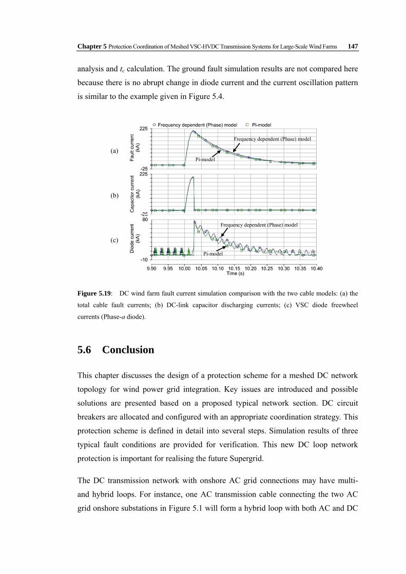
Chapter 5 Protection Coordination of Meshed VSC-HVDC Transmission Systems for Large-Scale Wind Farms 147
analysis and tc calculation. The ground fault simulation results are not compared here
because there is no abrupt change in diode current and the current oscillation pattern
is similar to the example given in Figure 5.4.
Frequency dependent (Phase) model
Pi-model
Frequency dependent (Phase) model
Pi-model
Figure 5.19: DC wind farm fault current simulation comparison with the two cable models: (a) the
total cable fault currents; (b) DC-link capacitor discharging currents; (c) VSC diode freewheel
currents (Phase-a diode).
5.6 Conclusion
This chapter discusses the design of a protection scheme for a meshed DC network
topology for wind power grid integration. Key issues are introduced and possible
solutions are presented based on a proposed typical network section. DC circuit
breakers are allocated and configured with an appropriate coordination strategy. This
protection scheme is defined in detail into several steps. Simulation results of three
typical fault conditions are provided for verification. This new DC loop network
protection is important for realising the future Supergrid.
The DC transmission network with onshore AC grid connections may have multi-
and hybrid loops. For instance, one AC transmission cable connecting the two AC
grid onshore substations in Figure 5.1 will form a hybrid loop with both AC and DC
(a)
(b)
(c)

Chapter 5 Protection Coordination of Meshed VSC-HVDC Transmission Systems for Large-Scale Wind Farms 148
connections. The AC and DC CB coordination issue needs to be considered due to
the significant difference in operation time, as indeed does the protection influence
on other AC CBs located around the onshore substations. Moreover, accurate and fast
ground distance evaluation and grounding resistance assessment method is required
for real-time coordination application.

Chapter 5 Protection Coordination of Meshed VSC-HVDC Transmission Systems for Large-Scale Wind Farms 149
5.7 References
[5.1] S. Gordon, “Supergrid to the rescue,” Power Engineer, vol. 20, no. 5, pp. 30-33, Oct./Nov. 2006.
[5.2] T. Ackermann, “Transmission system for offshore wind farms,” IEEE Power Engineering Review, pp. 23-27, Dec. 2002.
[5.3] N. Flourentzou, V. G. Agelidis, and G. D. Demetriades, “VSC-based HVDC power transmission systems: an overview,” IEEE Trans. Power Electron., vol. 24, no. 3, pp. 592-602, Mar. 2009.
[5.4] P. Bresesti, W. L. Kling, R. L. Hendriks, and R. Vailati, “HVDC connection of offshore wind farms to the transmission system,” IEEE Trans. Energy Convers., vol. 22, no. 1, pp. 37-43, Mar. 2007.
[5.5] D. Jovcic and N. Strachan, “Offshore wind farm with centralised power conversion and DC interconnection,” IET Gener. Transm. & Distrib., vol. 3, no. 6, pp. 586-595, Jun. 2009.
[5.6] P. M. Anderson, Power system protection. New York: IEEE Press, 1999.
[5.7] F. Lu, “Novel method for determining the optimal coordination sequence of directional relays in a complicated multi-loop power network based on coordination relationships between relays,” Journal of Automation of Electric Power Syst., vol. 29, no. 24, Dec. 2005.
[5.8] Q. Yue, F. Lu, W. Yu, and J. Wang, “A novel algorithm to determine minimum break point set for optimum cooperation of directional protection relays in multiloop networks,” IEEE Trans. Power Del., vol. 21, no. 3, pp. 1114-1119, Jul. 2006.
[5.9] M. Chinchilla, S. Arnaltes, and J. C. Burgos, “Control of permanent-magnet generators applied to variable-speed wind-energy systems connected to the grid,” IEEE Trans. Energy Convers., vol. 21, no. 1, pp. 130-135, Mar. 2006.
[5.10] M. E. Baran and N. R. Mahajan, “Overcurrent protection on voltage-source-converter-based multiterminal DC distribution systems,” IEEE Trans. Power Del., vol. 22, no. 1, pp. 406-412, Jan. 2007.
[5.11] D. Jovcic, and B. T. Ooi, “Developing dc transmission networks using dc transformers,” IEEE Trans. Power Del., vol. 25, no. 4, pp. 2535-2543, Oct. 2010.
[5.12] X. Liu, A. H. Osman, and O. P. Malik, “Hybrid travelling wave/boundary protection for monopolar HVDC line,” IEEE Trans. Power Del., vol. 24, no. 2, pp. 569-578, Apr. 2009.
[5.13] B. Gustavsen, G. Irwin, R. Mangelrod, D. Brandt, and K. Kent, “Transmission line models for the simulation of interaction phenomena between parallel ac and dc

Chapter 5 Protection Coordination of Meshed VSC-HVDC Transmission Systems for Large-Scale Wind Farms 150
overhead lines,” Int. Conf. on Power Sys. Transients, Budapest, Hungary, 20-24 Jun. 1999.
[5.14] IEEE Standard 551, Chapter 7, Capacitor contributions to short-circuit currents, IEEE recommended practice for calculating short-circuit currents in industrial and commercial power systems, Oct. 2006.
[5.15] F. Mura, C. Meyer, and R. W. De Doncker, “Stability analysis of high-power dc grids,” IEEE Trans. Ind. Appl., vol. 46, no. 2, pp. 584-592, Mar./Apr. 2010.
[5.16] A. Ametani, “A general formulation of impedance and admittance of cables,” IEEE Trans. Power Apparatus and Sys., vol. PAS-99, no. 3, 902-910, May/Jun. 1980.
[5.17] W. Hu, Z. Chen, Y. Wang, and Z. Wang, “Flicker mitigation by active power control of variable-speed wind turbines with full-scale back-to-back power converters,” IEEE Trans. Energy Convers., vol. 24, no. 3, pp. 640-649, Sep. 2009.
151
Chapter 6 Reliability Enhancement of Offshore Wind Farms by Redundancy Analysis
6.1 Introduction
The optimisation of the wind power collection grid design aims to minimise
large-scale offshore wind farms’ influence on the main network. Therefore, the
reliability of offshore wind farms needs to be assessed in detail because of the time-
and financial- aspects of construction and maintenance access issues in the offshore
environment. The wind farm reliability is distributed between the wind turbines, the
wind power generation systems, and the collection and transmission systems [6.1].
However, detailed large-scale offshore wind farm failure statistics are lacking due to
the short time of operational experiences [6.2]. Nevertheless, with the increasing
capacity of wind farms in planning and construction, also the requirements of fault
ride-through (FRT) capability to wind power generation systems from grid codes of
many countries [6.3], it is quite urgent to enhance the reliability and system stability
study of wind farm collection and transmission systems.
In terms of existing wind farm operational experience and wind farm failure survey,
this chapter firstly discusses the topology and assessment of reliability for collection
and transmission systems. Reliability is defined by taking into account the total
curtailed power during fault conditions, device failure rate, and mean time to repair
(MTTR), i.e. disrupted time.
Redundancy is a major way to enhance reliability of onshore distribution and
transmission systems. In this chapter, redundancy degree for offshore wind farms is
defined considering the redundant device voltage level, redundant cable to normal
cable route ratio and redundant devices. The basis of redundant decision-making is

Chapter 6 Reliability Enhancement of Offshore Wind Farms by Redundancy Analysis 152
the operational experience of existing offshore wind farms, and the estimated cost
data. The proposed method is used for an example practical offshore wind farm
scenario. Optimal redundancy design can be achieved with the discussion of
enhanced reliability and acceptable economic costs.
6.2 Wind Farm Collection/Transmission Systems and
Reliability
6.2.1 Collection Grids
The system of offshore transformers and linking cables are called collection grids
[6.4]−[6.6], or collector/collection systems [6.2], [6.7], [6.8]. Like onshore
distribution network, the optimal voltage level for offshore wind farm is the medium
voltage level, e.g. 33 kV in UK, in order to make a trade-off between the costs and
technical performance.
(a) (b)
Figure 6.1: (a) Horns Rev offshore wind farm (Denmark, built in 2002) [6.10]; (b) North Hoyle
offshore wind farm (UK, in full operation since 2003) [6.11].
1) Transformer Platform Location(s):
For transformer platforms, most of the existing studies assume that the platform is
outside the wind farm region. Reference [6.9] proposes an optimisation method for
locating the transformer platform. The principal objective of the optimisation process
is to minimise the total cable resources used to connect turbines to the transformer

Chapter 6 Reliability Enhancement of Offshore Wind Farms by Redundancy Analysis 153
platforms. The predictable result is that the geometric centre is the optimal position.
However, platform outside the wind farm region is simple for consideration, easy for
onshore connection, and is the case for almost all the existing offshore wind farms.
Figure 6.1 shows two offshore wind farm collection grids. Figure 6.1(a) is the
world’s first offshore wind farm – Horns Rev offshore wind farm in Denmark. Figure
6.1(b) is the North Hoyle offshore wind farm built in the UK, with redundant cables.
2) Wind Turbine Connections:
Wind turbines in a wind farm are always divided into several groups, in connection
forms of string or star. For star connection, the wind turbines in a star always share
one common transformer to reduce space and investment. While for string
connection, the wind turbines in a string have their own dedicated nacelle
transformers. In fact, they are unanimously necessary. Therefore, most studies
focused on the detailed string configurations, in which strings are commonly merged
into pairs, so-called “forks” [6.6] as shown in Figure 6.1(a). However, there is no
topology analysis in terms of the whole collection grids.
6.2.2 Transmission Systems
As discussed in the Chapter 1 literature review, the main decisions for the
transmission system to the onshore grid are voltage level and whether the system is
AC or DC. For reasons of transmission efficiency, it is always with a high voltage.
This is similar to the onshore transmission system. AC or DC transmission is a major
discussion until now. Because of the relatively high costs of high-voltage
direct-current (HVDC) converters and switchgear, and spacious transformer
platforms, AC transmission is preferable in current wind farm constructions, also
owing to its mature technologies and operational experiences [6.12], [6.13]. However,
the major disadvantage of AC transmission is the charging of cables so that there is a
distance limit for power delivery. With larger offshore wind farms and greater
distance from the grid, HVDC is promising for future wind farm power
transmissions.
Chapter 6 Reliability Enhancement of Offshore Wind Farms by Redundancy Analysis 154
6.2.3 Wind Farm Collection and Transmission System Reliability Assessment
The probabilistic reliability index, expected energy not served (EENS), is used to
assess the reliability of distribution and transmission systems [6.14]. It gives a
measure of the amount of power to deliver that can be curtailed during fault
conditions. Here the EENS of wind farm collection and transmission systems is
defined as [6.4]
( )∑=
××=N
iiii MTTRPqEENS
1
(MWh/year) (6.1)
where N is the total number of components (including medium-voltage circuit
breakers, disconnectors, switches, nacelle transformers, and cables). For component
indexed i, qi is the expected failure rate (frequency per year); Pi is the unavailable
installed power during its failures; MTTRi is its mean time to repair.
6.3 Wind Farm Collection and Transmission System
Redundancy Definition
There is no clear redundancy definition for wind farm collection and transmission
systems since wind farm redundancy is still not well studied. In this section, after
analysing existing redundancy choices, by dividing wind farm components into
different levels, the redundancy definition of the wind farm system is given. It is the
redundancy of collection grids, i.e. the power transmission between turbines and
turbine-to-platform cables that requires detailed discussion. One aspect of
redundancy concerns the topology. This means the energy that can flow through
different paths during faults, instead of being interrupted. Another is in respect of the
configuration of switchgear.
6.3.1 Topology Redundancy
Network topology generally includes redundancy. For main grids, this is referred to
the power transmission capacity of cables/lines. Conventional transmission grids are
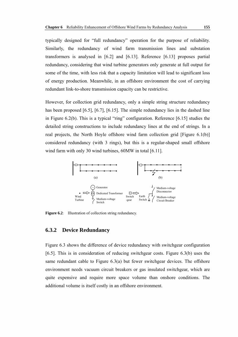
Chapter 6 Reliability Enhancement of Offshore Wind Farms by Redundancy Analysis 155
typically designed for “full redundancy” operation for the purpose of reliability.
Similarly, the redundancy of wind farm transmission lines and substation
transformers is analysed in [6.2] and [6.13]. Reference [6.13] proposes partial
redundancy, considering that wind turbine generators only generate at full output for
some of the time, with less risk that a capacity limitation will lead to significant loss
of energy production. Meanwhile, in an offshore environment the cost of carrying
redundant link-to-shore transmission capacity can be restrictive.
However, for collection grid redundancy, only a simple string structure redundancy
has been proposed [6.5], [6.7], [6.15]. The simple redundancy lies in the dashed line
in Figure 6.2(b). This is a typical “ring” configuration. Reference [6.15] studies the
detailed string constructions to include redundancy lines at the end of strings. In a
real projects, the North Hoyle offshore wind farm collection grid [Figure 6.1(b)]
considered redundancy (with 3 rings), but this is a regular-shaped small offshore
wind farm with only 30 wind turbines, 60MW in total [6.11].
• • • • • • • • • • • • • •
(a)
• • • • • • • • • • • • • •
(b)
Generator
Dedicated Transformer
Medium-voltage Switch
~
• Medium-voltage Disconnector
Medium-voltage Circuit Breaker
Earth Switch
Wind Turbine
Switch -gear
Figure 6.2: Illustration of collection string redundancy.
6.3.2 Device Redundancy
Figure 6.3 shows the difference of device redundancy with switchgear configuration
[6.5]. This is in consideration of reducing switchgear costs. Figure 6.3(b) uses the
same redundant cable to Figure 6.3(a) but fewer switchgear devices. The offshore
environment needs vacuum circuit breakers or gas insulated switchgear, which are
quite expensive and require more space volume than onshore conditions. The
additional volume is itself costly in an offshore environment.

Chapter 6 Reliability Enhancement of Offshore Wind Farms by Redundancy Analysis 156
• • • • • • •• • • • • • •
(a)
• • • • • • • • • • • • • •
(b)
Figure 6.3: Illustration of device redundancy of collection string switchgear configuration.
Another kind of device redundancy is the transformer redundancy used in grid
transmission systems. In substations, 2×70% total load capacity transformers are
usually used instead of 1×100%. In this case, when one transformer needs to be
repaired, there will still be 70% power supplied to customers, instead of losing all the
supply with only one substation transformer.
6.3.3 Redundancy Definition
Redundancy of the wind farm collection and transmission systems is divided into
three levels: collection grid level, platform level, and transmission level.
1) Collection Grid Level – Level 1:
As mentioned above, this level has both topology and device redundancy. In the
collection grid, here are two kinds of redundant branches: between wind turbines,
and between wind turbines and transformer platforms. Here only non-overlap
redundant branches are considered (connecting wind turbine points without blocking
or overlaying other branches), because in this condition the existing normal operation
branches can be fully used (included in the new operational states after fault
conditions). Each redundant branch needs switchgear and a protection relay system.
In this chapter, the redundancy definition is based on the typical string-radial
connection. For each string, usually there will be fewer than 10 wind turbines
connected, considering the power limit of submarine cables and the turbine capacity.
Example collection grids with 28 turbines in a rectangular area, and their redundant
connections are shown in Figure 6.4.
The turbine-platform redundant branch depends on the location of platforms due to
the string distribution. Figure 6.4 (a) and (b) illustrate two different string
connections with different platform location. The normal operation branch numbers
nnorm are both 28.

Chapter 6 Reliability Enhancement of Offshore Wind Farms by Redundancy Analysis 157
• • • • • • • • • • • • • • • • • • • • • • • • • • • •
• • • • • • • • • • • • • •
• • • • • • •
• • • • • • •
(a) (b)
• • • • • • • • • • • • • • • • • • • • • • • • • • • •
• • • • • • •
• • • • • • • • • • • • • •
• • • • • • •
(c) (d)
Normal design branches Redundant branches
Figure 6.4: Illustration of redundancy allocation: (a) left-side platform with 4 string connection,
with redundancy; (b) bottom-side platform with 4 string connection, with redundancy; (c) switchgear
distribution; (d) with long redundant cable.
The number of redundant branches nr can represent the redundancy degree. To
normalise, this number is divided by the normal operation branch number, to give the
redundancy degree parameter
γ1 = 1 + nr / nnorm. (2)
So in the examples of Figure 6.4(a) and (b), the redundancy parameters are γ1(a) =
1+6/28 ≈ 1.21, and γ1(b) = 1+7/28 ≈ 1.25.
The existence of redundant branch switchgear makes the switchgear distribution
different. Obviously, each redundant branch should have a switchgear system, and
also for the strings to connect to the collection transformer, as shown in Figure 6.4(c).
No more switchgear is required in normal branches. For the case of Figure 6.4(d),
there is one redundant branch much longer than normal-size. This redundancy
structure is proposed in [6.8]. Here this case is considered by the length nlong ≈ 6. Use
the normal-size branch cost CNB and switchgear cost CSW, so as to equivalence it into
a normal-sized branch-switchgear pair.
SWNB
NBlongequ CC
Cnn+
= . (6.3)

Chapter 6 Reliability Enhancement of Offshore Wind Farms by Redundancy Analysis 158
If CNB/CSW = 3, nequ = 6×3/4 = 4.5, γ1(c) = 1+(4.5+4)/28 ≈ 1.30.
It seems simple to introduce redundant branches to strings because the only
difference that can be made is whether to put a redundancy line there. In practice, for
large-scale systems the redundancy can be much more complex. Like the case of
Gwynt y Môr offshore wind farm [Figure 6.5, submitted in November 2005,
consented in December 2008], the irregular layout and flexible location of
transformer platforms make things intangible. Therefore, using a systematic
approach to optimise collection grid planning/design can substantially decrease the
amount of cost incurred.
DWF
DS x
y
Figure 6.5: The layout features of Gwynt y Môr offshore wind farm (background picture from
[6.16]).
In this complex scenario, the wind turbine of one group can be connected to the
transformer or a turbine of another group. The wind turbines at each string terminal,
if close to the other transformer platform, can be connected to it as a backup. This
influence will lead to the change of γ1 as
∑∑=
−=
⎟⎠
⎞⎜⎝
⎛++=
G
iinormgg
G
iri nnn
1,
11 21γ (6.4)
where G is the group number; nri, nnorm, and ng-g are the redundant, normal, and
group-to-group branch numbers respectively. The number 2 means the
group-to-group redundant branch introduces redundancy to both groups.
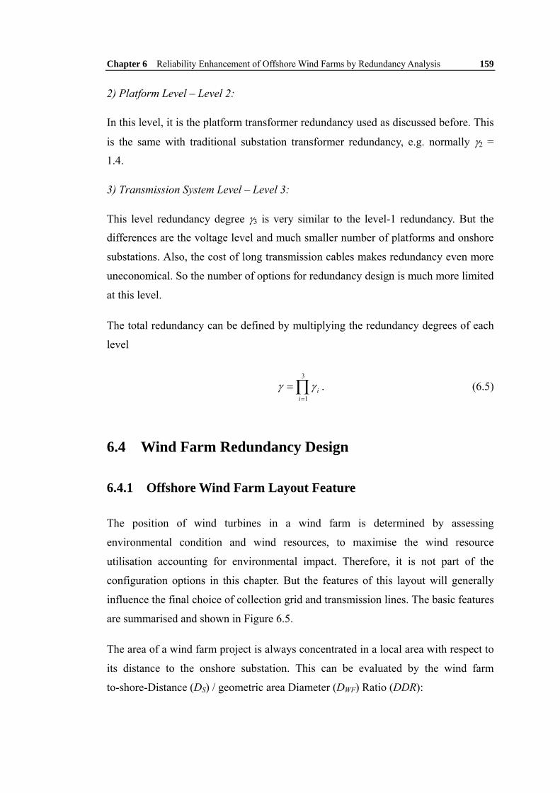
Chapter 6 Reliability Enhancement of Offshore Wind Farms by Redundancy Analysis 159
2) Platform Level – Level 2:
In this level, it is the platform transformer redundancy used as discussed before. This
is the same with traditional substation transformer redundancy, e.g. normally γ2 =
1.4.
3) Transmission System Level – Level 3:
This level redundancy degree γ3 is very similar to the level-1 redundancy. But the
differences are the voltage level and much smaller number of platforms and onshore
substations. Also, the cost of long transmission cables makes redundancy even more
uneconomical. So the number of options for redundancy design is much more limited
at this level.
The total redundancy can be defined by multiplying the redundancy degrees of each
level
∏=
=3
1iiγγ . (6.5)
6.4 Wind Farm Redundancy Design
6.4.1 Offshore Wind Farm Layout Feature
The position of wind turbines in a wind farm is determined by assessing
environmental condition and wind resources, to maximise the wind resource
utilisation accounting for environmental impact. Therefore, it is not part of the
configuration options in this chapter. But the features of this layout will generally
influence the final choice of collection grid and transmission lines. The basic features
are summarised and shown in Figure 6.5.
The area of a wind farm project is always concentrated in a local area with respect to
its distance to the onshore substation. This can be evaluated by the wind farm
to-shore-Distance (DS) / geometric area Diameter (DWF) Ratio (DDR):

Chapter 6 Reliability Enhancement of Offshore Wind Farms by Redundancy Analysis 160
DDR = DS / DWF. (6.6)
The distance between wind turbines are represented by a parallelogram with x, y as
side lengths (normally x = y).
6.4.2 The Design Process Description
The proposed optimisation procedure is illustrated in Figure 6.6. First, based on the
fixed wind farm layout, choose transformer platform location(s). Second, design the
normal operation string structure with cost limit consideration as traditional works.
Third, in three levels (collection grid, platform, and transmission system), perform
redundancy design. After the analysis of reliability and economic cost assessment
comes the study of the optimal redundancy degree with detailed redundancy
configuration.
Collection grid design
Choice of transformer platform location(s)
Optimal wind farm
Normal strings Redundant branchesReliability & Economic assessment
Given geographical wind farm array layout analysis
Cable routes Switchgear locations
Transmission system design
Figure 6.6: Flow chart of wind farm design process.
6.4.3 Choice of Transformer Platform Number and Location
The choice of appropriate platform number and location depends on the total number
of wind turbines and the required capacity of the transformers.
1) Number of Platforms:
The transformer platforms can also have redundancy, but due to the cost of building
platforms and the space limit, platform number redundancy is not considered here.
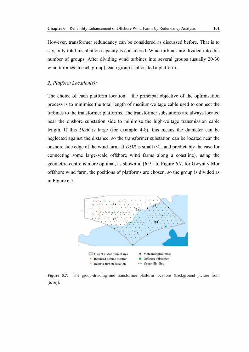
Chapter 6 Reliability Enhancement of Offshore Wind Farms by Redundancy Analysis 161
However, transformer redundancy can be considered as discussed before. That is to
say, only total installation capacity is considered. Wind turbines are divided into this
number of groups. After dividing wind turbines into several groups (usually 20-30
wind turbines in each group), each group is allocated a platform.
2) Platform Location(s):
The choice of each platform location – the principal objective of the optimisation
process is to minimise the total length of medium-voltage cable used to connect the
turbines to the transformer platforms. The transformer substations are always located
near the onshore substation side to minimise the high-voltage transmission cable
length. If this DDR is large (for example 4-8), this means the diameter can be
neglected against the distance, so the transformer substation can be located near the
onshore side edge of the wind farm. If DDR is small (<1, and predictably the case for
connecting some large-scale offshore wind farms along a coastline), using the
geometric centre is more optimal, as shown in [6.9]. In Figure 6.7, for Gwynt y Môr
offshore wind farm, the positions of platforms are chosen, so the group is divided as
in Figure 6.7.
(1) (3)
(2)
(4)
(5)
(6)
Gwynt y Môr project areaRequired turbine locationReserve turbine location
Meteorological mastOffshore substationGroup-dividing
Figure 6.7: The group-dividing and transformer platform locations (background picture from
[6.16]).
Chapter 6 Reliability Enhancement of Offshore Wind Farms by Redundancy Analysis 162
6.4.4 Normal Collection Grid Topology Design
The collection grid is firstly designed without redundancy. For each group, the wind
turbine is connected to platforms in strings to form a radial tree system. There has
been research about normal collection grid topology design, including normal
optimisation method [6.9] and genetic algorithms (GA) method [6.17]. The former is
used here. The strings can be evolved from the substations as trees including the
shortest distance from each wind turbine to the next point (substation or wind
turbine). Normally, each string includes less than 10 wind turbines. Figure 6.8 and
Table 6.1 show an example of normal collection grid design.
(1)
(3)
(2)
(4)
(5)
(6)
Figure 6.8: Normal collection grid string design.
Table 6.1: Group Division and Normal Collection Grid Design
Group WTG No. Normal Branch No. nnorm Group WTG No. Normal Branch No. nnorm
1 25 25 4 22 22
2 25 25 5 23 23
3 27 27 6 28 28
Total 250 250
6.4.5 Redundancy Design
1) Collection Grid Level – Level 1:
First, connect the platform to the nearest turbines of a neighbour group, if they are
not in a same string. The cable loading is limited to connecting 10 turbines.

Chapter 6 Reliability Enhancement of Offshore Wind Farms by Redundancy Analysis 163
Therefore, then connect the terminal turbine in a string with the smallest number of
turbines to the neighbour group with almost 10 turbine in its string. During this
process, the redundant branch should not be longer than 2x.
Each group itself requires redundancy. This is similar to traditional string redundancy
study, but much more flexible with the above among-group redundancies. After the
group-to-group connection, the objective of this step is to make sure each turbine has
two connections. So it is required to check turbines with only one connection, and
then connect it to the nearest turbine. For example, in Figure 6.9, if there are 13
group-to-group branches, for each group, the redundant branch number is nr1 = 6, nr2
= 4, nr3 = 4, nr4 = 2, nr5 = 3, nr6 = 4. In this condition, all the normal branches can be
switched out without any power curtailed. The redundancy parameter γ1 becomes
1.196, which is the maximum level-1 redundancy in this example. The final
collection grid design is shown in Figure 6.9. Longer redundant lines (>2x) are not
preferable in this case.
(1)
(3)
(2)
(4)
(5)
(6)
Normal design branchesGroup-to-group redundant branches
Inner-group redundant branches
Figure 6.9: Collection grid redundancy design, γ1 = 1.196.
2) Platform Level – Level 2:
As mentioned previously, the redundancy degree γ2 = 1 to 1.4.
3) Transmission System Level – Level 3:
Figure 6.10 shows the normal transmission cables and potential redundant cable
routes in the example wind farm.

Chapter 6 Reliability Enhancement of Offshore Wind Farms by Redundancy Analysis 164
9.5 km
3 km 3.75 km 6.5 km 2.5 km
4.5 km 6.75 km
3.25 km
5 km
7 km
14.5 km
13 km 17.25 km
Normal design cables Potential redundant cable routes
Figure 6.10: Transmission system design (background picture from [6.16]).
The transmission cables are also firstly designed without redundancy and then the
redundant transmission cables chosen. If the DDR is very small, and if there are
many large-scale offshore wind farms close to each other, the “Supergrid” can be
economically realised. So in terms of voltage level, the redundancy degree ranges
from “Supergrid” – to connect the wind farms along one coastline area together to
make a high voltage network – to only adding medium voltage redundant lines
between wind turbine strings, as shown in Figure 6.10.
6.5 Example Wind Farm Design Analysis
The above Gwynt y Môr offshore wind farm is used as the example system for the
proposed design method. The total power capacity will be 750 MW. Here choosing 3
MW wind turbines for the wind farm, there are 250 turbines in total, as shown in
Figure 6.7. For the layout feature, here use x = y = 1 km. DDR is about 1.03 due to
the given DS (about 17.5 km) and DWF (about 17 km).

Chapter 6 Reliability Enhancement of Offshore Wind Farms by Redundancy Analysis 165
6.5.1 Reliability Assessment
The reliability is assessed by EENS defined in (6.1). The failure rates and MTTR for
offshore wind farm devices are listed in Table 6.2.
Table 6.2: Failure Rates and MTTR for Offshore Wind Farm Devices [6.4]
Offshore Wind Farm Component Failure Rate qi (per year) MTTRi (h)
Nacelle transformer 0.0131 240
120 m tower cable 0.015 (per km) 240
Wind turbine tower
Medium-voltage switch 0.025 240
Medium-voltage circuit breaker 0.025 240
Medium-voltage disconnector 0.025 240
Collection grid
Medium-voltage submarine cable 0.015 (per km) 1440
Platform Transformer 0.0131 240
Transmission system High-voltage submarine cable 0.015 (per km) 1440
6.5.2 Economic Assessment
The detailed device cost information is usually confidential, so here the estimated
split construction expenditure of North Hoyle offshore wind farm is used, Tables 6.3
and 6.4. Considering the device difference and number of devices in Table 6.4, an
estimate of the per unit device costs for Gwynt y Môr wind farm is listed in Table
6.5.
Table 6.3: North Hoyle Offshore Wind Farm Information [6.18]
Component Attribute Quantity
Wind Turbine Generators (WTGs) Vestas V80, 2 MW 30
Transmission cables (2) Diameter 139 mm, 37 kg/m 10.781 km, 13.176 km Cable
Collection grid cables Diameter 105 mm, 21 kg/m 350 m (North-south) 800 m (East-west)
Wind farm area 10 km2
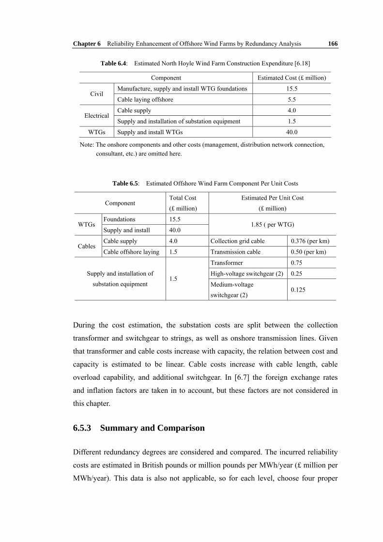
Chapter 6 Reliability Enhancement of Offshore Wind Farms by Redundancy Analysis 166
Table 6.4: Estimated North Hoyle Wind Farm Construction Expenditure [6.18]
Component Estimated Cost (£ million)
Manufacture, supply and install WTG foundations 15.5 Civil
Cable laying offshore 5.5
Cable supply 4.0 Electrical
Supply and installation of substation equipment 1.5
WTGs Supply and install WTGs 40.0
Note: The onshore components and other costs (management, distribution network connection, consultant, etc.) are omitted here.
Table 6.5: Estimated Offshore Wind Farm Component Per Unit Costs
Component Total Cost (£ million)
Estimated Per Unit Cost (£ million)
Foundations 15.5 WTGs
Supply and install 40.0 1.85 ( per WTG)
Cable supply 4.0 Collection grid cable 0.376 (per km) Cables
Cable offshore laying 1.5 Transmission cable 0.50 (per km)
Transformer 0.75
High-voltage switchgear (2) 0.25 Supply and installation of substation equipment
1.5 Medium-voltage switchgear (2)
0.125
During the cost estimation, the substation costs are split between the collection
transformer and switchgear to strings, as well as onshore transmission lines. Given
that transformer and cable costs increase with capacity, the relation between cost and
capacity is estimated to be linear. Cable costs increase with cable length, cable
overload capability, and additional switchgear. In [6.7] the foreign exchange rates
and inflation factors are taken in to account, but these factors are not considered in
this chapter.
6.5.3 Summary and Comparison
Different redundancy degrees are considered and compared. The incurred reliability
costs are estimated in British pounds or million pounds per MWh/year (£ million per
MWh/year). This data is also not applicable, so for each level, choose four proper

Chapter 6 Reliability Enhancement of Offshore Wind Farms by Redundancy Analysis 167
values to compare with the required extra device costs. The extra device quantity,
redundancy degree, increased cost and EENS costs are shown below: Level 1 − Table
6.6 and Figure 6.11, Level 2 − Figure 6.12, Level 3 − Table 6.7 and Figure 6.13.
Table 6.6: Level 1 - Device Cost Increase and EENS with Different Redundancy
ng-g nr γ1 Cost Increase (£ million) EENS (MWh/year)
0 0 1.000 0 70662
2 4 1.032 4.506 52632
4 7 1.060 8.511 40602
5 9 1.076 11.216 33504
7 12 1.104 13.719 24774
10 18 1.152 17.728 12622
13 23 1.196 21.036 4470
ng-g – the number of group-to-group redundant cables;
nr – the number of inner group redundant cables.
1 1.05 1.1 1.15 1.20
5
10
15
20
25
30
35
40
Redundancy degree
Cost
Incr
ease
and
Rel
iabi
lity
Costs
(£ m
illio
n)
Device Cost Increase£200 per MWh/year £250 per MWh/year£333 per MWh/year£500 per MWh/year
γ1
Figure 6.11: Collection grid level – level 1 cost and reliability analysis (different £ per MWh/year
values represent different conditions of cost incurred on average for an MWh loss per year).

Chapter 6 Reliability Enhancement of Offshore Wind Farms by Redundancy Analysis 168
1 1.05 1.1 1.15 1.2 1.25 1.3 1.35 1.40
0.5
1
1.5
2
2.5
Redundancy degree
Cost
Incr
ease
and
Rel
iabi
lity
Costs
(£ m
illio
n)
Device Cost Increase£20 per MWh/year£50 per MWh/year£100 per MWh/year£200 per MWh/year
γ2
Figure 6.12: Platform transformer level – level 2 cost and reliability analysis (different £ per
MWh/year values represent different conditions of cost incurred on average for an MWh loss per
year).
Table 6.7: Level 3 - Device Cost Increase and EENS with Different Redundancy
Redundant Cable length (km)
Switchgear No.
γ1 Cost Increase
(£ million) EENS
(MWh/year)
0 0 1.000 0 282744
3.75 2 1.081 13.375 88269
11.50 4 1.234 20.750 9600
22.25 8 1.455 41.906 0
1 1.1 1.2 1.3 1.4 1.50
20
40
60
80
100
Redundancy degree
Cost
Incr
ease
and
Rel
iabi
lity
Costs
(£ m
illio
n)
Device Cost Increase£50 per MWh/year£100 per MWh/year£200 per MWh/year£333 per MWh/year
γ3
Figure 6.13: Transmission system level – level 3 cost and reliability analysis (different £ per
MWh/year values represent different conditions of cost incurred on average for an MWh loss per
year).
Chapter 6 Reliability Enhancement of Offshore Wind Farms by Redundancy Analysis 169
Collection grid (level-1) redundancy design has many options so here we use seven
points; platform assessments (level-2) use two points to show the linear relationship;
for transmission system (level-3), due to the limited options, four points are shown.
From the above comparison, if the EENS loss information is available, the optimal
redundancy degree can be found at the point of reliability cost curve across the
increased device cost curve. The total maximal redundancy γ = 1.196×1.4×1.455 =
2.436 can be considered as the full redundancy condition.
In [6.19], it is mentioned that the fault likelihood and the associated costs are
assumed to be lower than the costs for the additional devices. Therefore, redundancy
is not taken into consideration. This may be true for small wind farms. But the
comparison results show that redundancy is necessary for large-scale offshore wind
farms due to economic aspects.
This systematic design method is in favour of comparing numerous options for
complex offshore wind farm electrical system design. In addition, the results of AC
and DC wind farms can be compared to explore the difference related to the diverse
cost distribution among equipment, foundations and space, and individual device
reliabilities. Hence it will be helpful for DC wind farm design, notwithstanding the
disadvantage of high-cost DC devices. However, key to this method is accurate
offshore wind farm operation statistics and detailed AC and DC equipment costs for
accurate optimisation results.
6.6 Conclusion
The growing scale of future offshore wind farms makes reliability enhancement
important during the planning and design phases. After analysing the importance and
necessity of redundancy in wind farm collection and transmission systems, a detailed
systematic redundancy design method is proposed and described from both technical
and economic standpoints. The syntheses of cost and reliability measures are defined.
The final degree of redundancy can be achieved using reliability and economic loss
statistics. Results show that the balance between reasonable investment in

Chapter 6 Reliability Enhancement of Offshore Wind Farms by Redundancy Analysis 170
redundancy and the reliability of offshore wind farms can be analytically reached.
More practical operational statistics and economic analysis are required for future
modern wind farm applications, especially for large-scale DC offshore wind farm
scenarios.

Chapter 6 Reliability Enhancement of Offshore Wind Farms by Redundancy Analysis 171
6.7 References
[6.1] P. J. Tavner, J. Xiang, and F. Spinato, “Reliability analysis for wind turbines,” Wind Energy, in Wiley Interscience, vol. 10, pp. 1-18, 2007, [Online]. Available: http://www3.interscience.wiley.com/cgi-bin/fulltext/112701014/PDFSTART
[6.2] R. A Walling and T. Ruddy, “Economic optimization of offshore wind farm substations and collection systems,” 5th Int. Workshop on Large-Scale Integration of Wind Power and Trans. Networks for Offshore Wind Farms, Glasgow, UK, Apr. 7-8, 2005.
[6.3] A. I. Estanqueiro, J. M. Ferreira de Jesus, J. Ricardo, Amarante dos Santos, and J. A. Peças Lopes, “Barriers (and solutions...) to very high wind penetration in power systems,” in Proc. of IEEE Power Eng. Society General Meeting, Tampa, Florida, USA, Jun. 24-28, 2007.
[6.4] A. Sannino, H. Breder, and E. K. Nielsen, “Reliability of collection grids for large offshore wind parks,” in Proc. of the 9th Int. Conf. Probabilistic Methods Appl. to Power Syst., Stockholm, Sweden, Jun. 11-15, 2006.
[6.5] B. Franken, H. Breder, M. Dahlgren, and E. K. Nielsen, “Collection grid topologies for off-shore wind parks,” in Proc. of the 18th Int. Conf. Electricity Distribution, Turin, Italy, Jun. 6-9, 2005.
[6.6] L. Liljestrand, A. Sannino, H. Breder, and S. Thorburn, “Transients in collection grids of large offshore wind parks,” Wind Energy, in Wiley Interscience, vol. 2, pp. 1-12, Jul. 2007, [Online]. Available: http://doi.wiley.com/10.1002/ we.233
[6.7] J. Green, A. Bowen, L. J. Fingersh, and Y. Wan, “Electrical collection and transmission systems for offshore wind power,” Offshore Technology Conference, Houston, Texas, USA, Apr. 30-May. 3, 2007. Available: http://www.nrel.gov/wind/pdfs/41135.pdf
[6.8] G. Quinonez-Varela, G. W. Ault, O. Anaya-Lara, and J. R. McDonald, “Electrical collector system options for large offshore wind farms,” IET Renew. Power Gener., vol. 1, no. 2, pp. 107-114, Jun. 2007.
[6.9] P. D. Hopewell, F. Castro-Sayas, and D. I. Bailey, “Optimising the design of offshore wind farm Collection networks,” in Proc. of the 41st International Universities Power Eng. Conf., pp. 84-88, Newcastle-upon-tyne, UK, Sep. 6-8, 2006.
[6.10] VATTENFALL Company. 2007. http://www.vattenfall.com/www/vf_com/vf_com/Gemeinsame_Inhalte/DOCUMENT /360168vatt/569396horn/P0277546.pdf
[6.11] Npower renewables. North Hoyle offshore wind farm. http://www.npower-renewables.com/northhoyle/components.asp

Chapter 6 Reliability Enhancement of Offshore Wind Farms by Redundancy Analysis 172
[6.12] H. Brakelmann, “Efficiency of HVAC power transmission from offshore-windmills to the grid,” IEEE PowerTech Conf., Bologna, Italy, Jun. 23-26, 2003.
[6.13] A. B. Morton, S. Cowdroy, J. R. A. Hill, M. Halliday, and G. D. Nicholson, “AC or DC? Economics of grid connection design for offshore wind farms,” in Proc. of the 8th IEE Int. Conf. on AC and DC Power Transmission, pp. 236-240, Melbourne, Vic., Australia, Mar. 28-31, 2006.
[6.14] J. Choi, T. D. Mount, R. J. Thomas, and R. Billinton, “Probabilistic reliability criterion for planning transmission system expansions,” IEE Proc. Gener. Trans. Distri., vol. 153, no. 6, pp. 719-727, Nov. 2006.
[6.15] P. Gardner, L. M. Craig, and G. J. Smith, “Electrical systems for offshore wind farms,” in Proc. of the 20th British Wind Energy Association Wind Energy Conf., Cardiff, UK, Sep. 1998.
[6.16] Npower renewables. Gwynt y Môr offshore wind farm. http://www.npower-renewables.com/gwyntymor/index.asp
[6.17] M. Zhao, Z. Chen, and J. Hjerrild, “Analysis of the behaviour of Genetic Algorithm applied in optimization of electrical system design for offshore wind farms,” in Proc. of 32nd Annual IEEE Conf. Ind. Electron., pp. 2335-2340, Paris, France, Nov. 6-10, 2006.
[6.18] J. M. F. Carter, “North Hoyle offshore wind farm: design and build,” Proc. of the Institution of Civil Engineers, Energy 160 Issue ENI, pp. 21-29, Feb. 2007. Available: http://www.atypon-link.com/doi/pdf/10.1680/ener.2007.160.1.21
[6.19] T. Ackermann, “Transmission system for offshore wind farms,” IEEE Power Engineering Review, vol. 22, no. 12, pp. 23-27, Dec. 2002.

173
Chapter 7 Conclusions and Future Work
7.1 Conclusions
Reliable protection systems for offshore wind farms are a prerequisite for the
development of this renewable energy industry. However, due to lack of operational
experience, this is a relatively new area of research. In this thesis, the protection
issues related to wind power generation systems, collection grids and transmission
systems are investigated. The contributions of this thesis in the context of wind
power system protection are summarised as follows.
• Detailed performance analyses during various fault conditions of two popular
variable-speed wind power generation systems – doubly-fed induction
generator (DFIG) (in Chapter 2) and permanent magnet synchronous generator
(PMSG) (in Chapter 3) are reported. Appropriate protection schemes are
proposed for different topologies in order to protect the vulnerable power
electronic converters. For DFIG, rotor overcurrent expressions are derived for
various fault conditions. Based on that, a new series dynamic resistor-based
protection circuit is proposed to protect the rotor-side converter without
short-circuiting the rotor winding. This is advantageous in avoiding grid
voltage deterioration from reactive power absorption, compared with
conventional crowbar protection. Used in line with the traditional crowbar and
DC-chopper protection, the proposed method can greatly enhance the DFIG
system fault ride-through capability. Comprehensive PSCAD/EMTDC
simulation studies are carried out as verifications. For PMSG, the protection
systems are aimed at reducing the DC-link overvoltages caused by interruption
Chapter 7 Conclusions and Future Work 174
of the power transmission route. Both large-scale and small-scale topologies are
studied for possible stand-alone or offshore applications. Series and parallel
topology and DC or AC side resistor allocation options are examined and
compared by simulation work. Application of pitch control for large-scale wind
turbine to reduce overspeed effect due to electrical faults is also included in
rotor shaft protection.
• The PMSG-based wind power generation system is expanded into a radial DC
wind farm. In terms of wind farm collection and transmission systems, DC
system protection schemes based on traditional AC network protection
principles are presented in Chapter 4. DC switchgear allocation is illustrated
with typical wind farm connection examples. The currently promising
voltage-source conversion technology is investigated in detail for fault
overcurrent analysis and critical stage definitions. This nonlinear system
analysis not only defines the most critical stages that need to be avoided, but
also instructs fault location. For small-scale radial wind farm collection systems,
a coordination method without using communication devices between distant
cable circuit breakers is proposed with a simple option of reverse-diode
protection. Based on the fault analysis, a fault location method for ground fault
conditions is proposed in particular. This fault location method is immune to
variations in the relatively large ground fault resistances, distances, and system
operation conditions, to effectively realise protection coordination.
• In Chapter 5, for large-scale wind farm integration, a typical meshed HVDC
transmission system section is presented for DC fault protection design and test,
in order to realise a reliable DC network for wind power connections. This
topology includes multi- onshore grid connections and loop cable routes.
Simulation system is built in PSCAD/EMTDC environment. With economic
uni-directional current-blocking power electronic circuit breakers, a new
protection coordination scheme is proposed for loop cable faults, radial cable
faults, and DC bus faults. Special coordination between circuit breakers at the
terminals of the same cable under DC bus faults is performed. Detailed

Chapter 7 Conclusions and Future Work 175
frequency dependent cable model is considered and compared with π-model
which is used for theoretical analysis. Results show that for fault conditions,
π-model is adequate for overcurrent analysis. The system reliability and power
delivery capability under fault conditions are improved by effective fault
isolation and possible loop power delivery routes.
• In Chapter 6, for the purpose of enhancing system reliability redundancy is
introduced into wind farm planning. Wind farm reliability and redundancy
degree are defined to describe a redundant system topology. After analysing the
importance and necessity of redundancy in wind farm collection and
transmission systems, a detailed systematic redundancy design method is
proposed and described from both technical and economic standpoints. The
final degree of redundancy is optimised using reliability economic loss
statistics. With reasonable investment in redundancy, the reliability of offshore
wind farms can be significantly improved.
In conclusion, the wind power generation system protection problems introduced in
this thesis and the solution investigations seek to contribute to both the understanding
and applications of protection in the field of large-scale offshore wind power
integration to existing onshore power networks. From the perspectives of individual
wind power generation systems, to an entire wind farm, even multiple large-scale
wind farm connection systems, the electrical fault analysis and protection issues are
discussed systematically. Future research aspects of this topic are discussed for the
promising high-power DC network applications.
7.2 Future Work
Possible future work is listed as follows:
• Experimental test rig for protection system design is required to verify the
protection schemes proposed in this thesis. However, this depends on the
effective fault simulation hardware for this potentially destructive experiment.

Chapter 7 Conclusions and Future Work 176
Real-time simulation software or real-time digital simulator (RTDS) are
possible ways to perform system fault and relay coordination simulation. For
computer simulation, appropriate simulation software or even development of
dedicated simulation modelling for fault analysis are required for efficient
large-scale system simulation and real-time applications. The analysis of
PMSG demagnetisation during fault conditions should be performed in detail as
well.
• Research on multi-terminal DC network for wind power collection and
transmission still requires more detailed work. In particular, the development
and implementation of fault tolerant high-power voltage-source converters, for
example those based on a multi-modular converter, and solid-state DC/DC
step-up converters, with high efficiency and power control performance could
be considered. For example, resonant converter applications for connection of
systems at different DC voltage levels.
• Reliable and high-current interruption performance DC circuit breakers based
on power electronic devices are urgently required. Detailed topology and
associated relay system design should be tested at realistic power levels. This is
prerequisite for application to large-scale DC networks in the future.
Appropriate fuse should also be chosen for DC application as backup for circuit
breaker switchgear systems.
• DC cable fault location methods should be tested with practical measurement
sensors to verify their robustness and accuracy thereby providing the possibility
of proposing improved algorithms. This is important for the industrial
application of the proposed fault location method.
• More specific and dedicated wind farm construction and operational cost
statistics and analysis are required for more accurate economic analysis and
general planning instruction, in order to make a reasonable balance between the
topology redundancy and system reliability. Wind power economics is a new
area of academic research.