Fast and Reliable Resampling Detection by SpectralAnalysis of Fixed Linear Predictor Residue

Matthias KirchnerInstitute for System ArchitectureTechnische Universität Dresden

01062 Dresden, Germanymatthias.kirchner@inf.tu-dresden.de

ABSTRACTThis paper revisits the state-of-the-art resampling detec-tor, which is based on periodic artifacts in the residue ofa local linear predictor. Inspired by recent findings fromthe literature, we take a closer look at the complex detec-tion procedure and model the detected artifacts in the spa-tial and frequency domain by means of the variance of theprediction residue. We give an exact formulation on howtransformation parameters influence the appearance of peri-odic artifacts and analytically derive the expected positionof characteristic resampling peaks. We present an equiva-lent accelerated and simplified detector, which is orders ofmagnitudes faster than the conventional scheme and exper-imentally shown to be comparably reliable.

Categories and Subject DescriptorsI.4.m [Image Processing]: Miscellaneous

General TermsAlgorithms, Security

Keywordsdigital image forensics, tamper detection, resampling detec-tion, predictor residuum, periodic artifacts

1. INTRODUCTIONOver the past years, research on digital image forensics

and tamper detection has become a hot topic in the multi-media security community [12]. A wide distribution of low-cost digital imaging devices and sophisticated image editingsoftware allow the production of image forgeries that are vir-tually indistinguishable from authentic photographs. Schol-ars in digital image forensics aim at restoring some of thelost trustworthiness to digital images by providing tools tounveil conspicuous traces of previous image manipulations.The key point of all image forensic methods is the absence

Permission to make digital or hard copies of all or part of this work forpersonal or classroom use is granted without fee provided that copies arenot made or distributed for profit or commercial advantage and that copiesbear this notice and the full citation on the first page. To copy otherwise, torepublish, to post on servers or to redistribute to lists, requires prior specificpermission and/or a fee.MM&Sec’08, September 22–23, 2008, Oxford, United Kingdom.Copyright 2008 ACM 978-1-60558-058-6/08/09 ...$5.00.

of any prior knowledge of the original image. This obviouslyproves to be beneficial in many practical applications wherethe original data is not directly accessible.

Amongst others, resampling detection has become a stan-dard tool for the forensic analysis of digital images. Thecreation of convincing image forgery oftentimes involves ge-ometric transformations, which typically comprise a resam-pling of the original image to a new sampling grid. The de-tection of resampling is therefore of particular interest andseveral schemes have been proposed to address this question.As a common ground, all these detectors exploit periodicinterpolation artifacts. While Popescu and Farid’s state-of-the-art detector [9], to the best of our knowledge also thefirst proposed technique, identifies such traces in the residueof a local linear predictor, more recent algorithms analyzethe variance of derivatives of a resampled image [2, 7, 11].

Inspired by these recent findings, in this paper, we willrevisit Popescu and Farid’s scheme and take a closer look atthe origin of periodic artifacts in the p-map of a resampledimage, which is the main output of the detector. A simpli-fied model based on the variance of the prediction residuewill serve as a tool to explain the actual appearance of thep-map and its spectral representation for arbitrary geomet-ric transformations. This goes beyond the original work ofPopescu and Farid, as they did not provide an explicit re-lation on how a particular transformation will influence thedetector’s output in the spatial and in the frequency do-main. In addition, we will present an accelerated version ofthe original detector which bypasses the most computation-ally demanding elements in the detection process and at thesame time provides equally reliable detection of resampling.

The rest of this paper is organized as follows. Section 2reviews the basic principles of resampling and the detectionalgorithm as proposed by Popescu and Farid. In Sect. 3 wewill model periodic artifacts in the p-map of a resampledsignal based on the variance of the residue of the employedlinear predictor and highlight implications on the detectionprocess. Before presenting our modified detector in Sect. 5,Section 4 addresses the localization of characteristic peaks ina p-map’s spectral representation. Section 6 finally reportsfirst experimental results before Sect. 7 concludes the paperand discusses implications on related fields.

2. DETECTION OF RESAMPLING

2.1 ResamplingOftentimes, the creation of convincing image forgery in-

volves scaling or rotation operations. In general, such ge-

ometric transformations imply a resampling of the origi-nal image [13], i.e., a mapping of discrete integer sourcecoordinates χ = (χ1, χ2) to real-valued target coordinatesx = (x1, x2) = Ψ(χ) according to a specified mapping func-tion Ψ : Z2 → R

2. In the course of this paper we will restrictourselves to the important class of affine transformations,

x = Aχ , (1)

where A is the 2 × 2 transformation matrix. Interpolationis the key to smooth and visually appealing image transfor-mation and can be written as

s(Aχ′) =Xχ∈Z2

s(χ)h(Aχ′ − χ) , (2)

where s is the signal of interest and h : R2 → R2 is the in-

terpolation kernel. Note that for notational convenience andwithout loss of generality we will focus our analysis on one-dimensional (1D) signals. Extensions to two-dimensional(2D) signals will be provided when necessary and/or use-ful. In the 1D case, resampling can be seen as a mappingbetween discrete source coordinates χ ∈ Z and target coor-dinates ωχ ∈ R, where ω > 0 is the inverse resampling rate.Equation (2) reduces to

s(ωχ′) =

∞Xχ=−∞

h(ωχ′ − χ)s(χ) , (3)

with ω < 1 for upsampling and ω > 1 for downsampling.

2.2 Detection of ResamplingA virtually unavoidable side effect of typical interpolation

algorithms is that they create linear dependencies betweengroups of neighboring samples. As shown by Gallagher [2]and Mahdian and Saic [7], the strength of dependence variesperiodically with the cycle length, which itself depends onthe resampling rate ω−1. To the best of our knowledge, allresampling detectors exploit these periodic artifacts, whichcan be found in the residuals of a local linear predictor [9]as well as in the derivatives of a resampled signal [2, 7, 11].

Popescu and Farid’s detector [9], probably the most exten-sively tested1 and most widely used method for resamplingdetection, employs a linear predictor to approximate eachsample’s value as the weighted sum of its 2K surroundingsamples,

s(ωχ′) =

KXk=−K

αks(ωχ′ + ωk) + e(ωχ′) with α0 := 0 . (4)

A so-called p-map as a measure for the strength of lineardependence is derived from the prediction error e, which ismodeled as a zero mean Gaussian random variable. Largeprediction errors indicate a minor degree of linear depen-dence and therefore result in small values in the p-map. Thecore of the detection procedure is a weighted least squares(WLS) estimation of the initially unknown scalar weightsα, incorporated into an iterative expectation maximization(EM) framework [1]. A stylized block diagram of the detec-tion process is given in Fig. 1.

Previous resampling operations leave conspicuous patternin the estimated p-map. The pattern becomes most evidentafter a transformation into the frequency domain, using a

1Test results for a wide variety of resampling parameterscan be found in [8].

α[0]calculate e and p-map p for currentestimate α[i]

compute α[i+1]

by minimizingPp(ωχ′)e(ωχ′)2

‖α[i+1] −α[i]‖ < ǫ ?

α = α[i+1]

p-map

yesno

i = i + 1

Figure 1: Iterative EM estimation of the predictionweights α.

Figure 2: Results of resampling detection for origi-nal image (top row) as well as 111 % and 150 % up-sampling (bottom rows). p-Maps are displayed inthe middle column. Periodic resampling artefactslead to characteristic peaks in the correspondingspectrum (rightmost pictures).

discrete Fourier transform (DFT), where it shows up as dis-tinct peaks that are characteristic for the resampling param-eters. The decision whether an image was resampled or notis made on the basis of this spectral representation, as themagnitude of distinct peaks can be easily measured in anautomated process.

Figure 2 presents some typical detection results for a greyscale image which has been scaled up to 111 % (ω = 0.9) and150 % (ω = 2/3) of the original (left column). The calculatedp-maps are displayed in the middle column. Note that onlyresampling causes strong periodic artifacts in the p-maps,resulting in very pronounced peaks in the spectrum.

3. ORIGIN OF PERIODIC ARTIFACTSAlthough the above described detection method is already

known as an effective and powerful tool, we believe that anin-depth analysis of the origin of the periodic artifacts in a

resampled image’s p-map can help to further clarify why therather complex detector works as it does.

Independent of Popescu and Farid’s work, Gallagher [2]noticed that the variance of the second order derivative ofan interpolated i.i.d. Gaussian signal is periodic with thesampling rate of the original signal. Only recently, Mahdianand Saic [7] gave an extended view and analytically showedthat, under a stationary signal model, the variance of then-th order derivative of a resampled signal is periodic withthe original sampling rate.

3.1 Periodic Artifacts of the Prediction ErrorTo get a better understanding of the actual output of

Popescu and Farid’s detector, we show the relation betweenthis method and the derivative-based approaches [2, 7] andtake a closer look at the prediction error, which is obviouslythe origin of periodic artifacts in the p-map of a resampledsignal. From Eq. (4), the residuum can be written as

e(ωχ′) = s(ωχ′)−KX

k=−Kαks(ωχ

′ + ωk) . (5)

Obviously, e(ωχ′) can be expressed solely in terms of originalsamples s(χ) by incorporating Eq. (3) as follows:

e(ωχ′) =

∞Xχ=−∞

h(ωχ′ − χ)s(χ)

−KX

k=−Kαk

∞Xχ=−∞

h(ωχ′ + ωk − χ)s(χ) (6)

Alternatively, we can write e(ωχ′) as a weighted sum of theactual sample of interest, s(ωχ′), and its surrounding 2Kneighbors,

e(ωχ′) =

KXk=−K

βk

∞Xχ=−∞

h(ωχ′ + ωk − χ)s(χ) , (7)

with weights β defined as

βk =

(1 for k = 0

−αk else.(8)

Finally, by interchanging the order of summation, the residuumbecomes

e(ωχ′) =∞X

χ=−∞ϕω(ωχ′ − χ)s(χ) , (9)

where function ϕω is defined as

ϕω(x) =

KXk=−K

βkh(x+ ωk) . (10)

Equation (9) reveals that e(x) is basically a linearly filteredversion of the original signal s(χ) with filter coefficients ϕωderived from weighted interpolation coefficients. Note thatEq. (9) is a generalization of Gallagher’s work [2], who gavean equivalent formula for a linear derivative filter.

From Eq. (9), we can compute the prediction error’s vari-ance Var[e(x)] as

Var[e(x)] =

∞Xχ=−∞

ˆϕω(x− χ)

˜2Var[s(χ)] +

+ 2

∞Xχ1=−∞

∞Xχ2=χ1+1

ϕω(x− χ1)ϕω(x− χ2) Cov[s(χ1), s(χ2)]

(11)

For our theoretical analysis we will assume s(χ) to be awide sense stationary signal2 with Var[s(χ)] = const andCov[s(χ1), s(χ2)] = Cov[s(χ1 + κ), s(χ2 + κ)].

Theorem 1. For wide sense stationary signals s(χ) withχ ∈ Z and Var[s(χ)] > 0 it holds for arbitrary predictionweights α 6= 0 and ∀x ∈ R that Var[e(x)] = Var[e(x+ 1)].

Proof. Let ∆(x) : R→ [0, 1) be a function defined as

∆(x) = x− bxc (12)

so that ∆(x) = ∆(x+ 1). We write Var[e(x)] as

Var[e(x)] =

∞Xχ=−∞

ϕ2ω(∆(x)− χ) Var[s(χ+ bxc)] +

+ 2

∞Xχ1=−∞

∞Xχ2=χ1+1

ϕω(∆(x)− χ1)ϕω(∆(x)− χ2)

Cov[s(χ1 + bxc), s(χ2 + bxc)] (13)

where ϕω(∆(x)−χ) = ϕω(∆(x+ 1)−χ). From Var[s(χ)] =const as well as Cov[s(χ1 + bxc), s(χ2 + bxc)] = Cov[s(χ1 +bx+1c), s(χ2 +bx+1c)] (stationarity assumption) it followsthat Var[e(x)] = Var[e(x+ 1)].

Basically, Theorem 1 states that for resampled station-ary and non-constant signals s(χ), χ ∈ Z, the variance ofa linear predictor’s residuum varies with a period of 1, in-dependent of the actual prediction weights. This specificperiodicity can be inferred from the convolutive nature ofkernel-based interpolation, which employs the very same in-terpolation weights to determine new samples at positionsx and x+ 1.With 1 being the original sampling rate, Theo-rem 1 shows a relation between the derivative-based detec-tion schemes and Popescu and Farid’s detector.

It is straightforward to show that Theorem 1 also holds fortwo-dimensional resampled stationary signals. In this case,Var[e(x1, x2)] is periodic in both dimensions, thus

Var[e(x1, x2)] = Var[e(x1 + 1, x2)] =

Var[e(x1, x2 + 1)] = Var[e(x1 + 1, x2 + 1)] . (14)

3.2 Why Periodic Variance MattersAs described in Sect. 2.2, Popescu and Farid’s detector

[9] models e(ωχ′) as a N (0, σ) Gaussian random variable.According to the employed model, larger prediction errorscorrespond to less linear dependence and thus yield smallervalues in the p-map. From Theorem 1 we can infer that thetheoretically derived variance of the prediction error peri-odically varies throughout the whole signal. Since a large

2This is a reasonable assumption especially for homogeneousparts of a signal.

0 1 2 3 4 5 6 7 8 9 10

0

0.2

0.4

0.6

0.8

1.0

1.2

x

Var[

e(x

)]

b

b b

b

b b

b

b b

b

b b

b

b b

b

b

b

b

b

b

b

b

b

b

b

b

b

b

b

b

b

b

b

b

b

b

b

b

b

b

bb

b

b

b

b

b

b

ω = 0.9

ω = 2/3

ω = 0.5

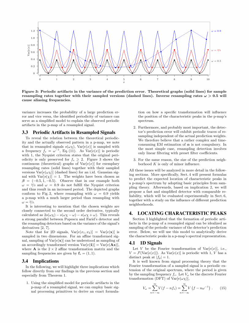
Figure 3: Periodic artifacts in the variance of the prediction error. Theoretical graphs (solid lines) for sampleresampling rates together with their sampled versions (dashed lines). Inverse resampling rates ω > 0.5 willcause aliasing frequencies.

variance increases the probability of a large prediction er-ror and vice versa, the identified periodicity of variance canserve as a simplified model to explain the observed periodicartifacts in the p-map of a resampled signal.

3.3 Periodic Artifacts in Resampled SignalsTo reveal the relation between the theoretical periodic-

ity and the actually observed pattern in a p-map, we notethat in resampled signals s(ωχ), Var[e(x)] is sampled witha frequency fs = ω−1, Eq. (11). As Var[e(x)] is periodicwith 1, the Nyquist criterion states that the original peri-odicity is only preserved for fs ≥ 2. Figure 3 shows thecontinuous (theoretical) graphs of Var[e(x)] for exemplaryresampling rates (solid lines) together with their sampledversions Var[e(ωχ)] (dashed lines) for an i.id. Gaussian sig-nal with Var[s(χ)] = 1. The weights have been chosen asβ = (−0.5, 1,−0.5). Observe that in our example bothω = 2/3 and ω = 0.9 do not fulfill the Nyquist criterionand thus result in an increased period. The depicted graphsconform to Fig. 2, where resampling with ω = 0.9 yieldsa p-map with a much larger period than resampling withω = 2/3.

It is interesting to mention that the chosen weights areclosely connected to the second order derivative, typicallycalculated as 2s(ωχ)− s(ωχ− ω)− s(ωχ+ ω). This revealsa strong parallel between Popescu and Farid’s detector andthe resampling detectors based on the variance of the signal’sderivatives [2, 7].

Note that for 2D signals, Var[e(x1, x2)] = Var[e(x)] issampled in two dimensions. For an affine transformed sig-nal, sampling of Var[e(x)] can be understood as sampling ofan accordingly transformed version Var[e(x)] = Var[e(Ax)],where A is the 2 × 2 affine transformation matrix and thesampling frequencies are given by fs = (1, 1).

3.4 ImplicationsIn the following, we will highlight three implications which

follow directly from our findings in the previous section andespecially from Theorem 1.

1. Using the simplified model for periodic artifacts in thep-map of a resampled signal, we can employ basic sig-nal processing primitives to derive an exact formula-

tion on how a specific transformation will influencethe position of the characteristic peaks in the p-map’sspectrum.

2. Furthermore, and probably most important, the detec-tor’s prediction error will exhibit periodic traces of re-sampling independent of the actual prediction weights.We therefore believe that a rather complex and time-consuming EM estimation of α is not compulsory. Inthe most simple case, resampling detection involvesonly linear filtering with preset filter coefficients.

3. For the same reason, the size of the prediction neigh-borhood K is only of minor influence.

All these issues will be analyzed in more detail in the follow-ing sections. More specifically, Sect. 4 will present formulasto predict the expected location of characteristic peaks ina p-map’s spectrum by adopting basic principles from sam-pling theory. Afterwards, based on implication 2, we willpropose a fast and simplified detector with comparable re-liability, which will be evaluated experimentally in Sect. 6,together with a study on the influence of different predictionneighborhoods.

4. LOCATING CHARACTERISTIC PEAKSSection 3 highlighted that the formation of periodic arti-

facts in the p-map of a resampled signal can be idealized assampling of the periodic variance of the detector’s predictionerror. Below, we will use this model to analytically derivethe characteristic peaks in a p-map’s spectral representation.

4.1 1D SignalsLet V be the Fourier transformation of Var[e(x)], i.e.,

V = F(Var[e(x)]). As Var[e(x)] is periodic with 1, V has adistinct peak at |fp| = 1.

It is well known from signal processing theory that theFourier transformation of a sampled signal is a periodic ex-tension of the original spectrum, where the period is givenby the sampling frequency fs. Let Vω be the discrete Fouriertransformation (DFT) of Var[e(ωχ)],

Vω =∞X

n=−∞V (f − nfs) =

∞Xn=−∞

V`f − nω−1´ . (15)

0

0.5

0 0.5 1.0 1.5 2.0 ω

|f ′c|

Figure 4: Normalized characteristic peak position|f ′c| for 1D resampling. Different inverse resamplingrates ω result in the same peak position.

The baseband of Vω is given by −1/2ω ≤ f ≤ 1/2ω. As wasalready mentioned in Sect. 3.3, “correct” sampling impliesfp ≤ 1/2ω and thus ω ≤ 0.5. In this case, the character-istic peaks in the p-map’s spectrum are directly given by±1. Otherwise aliasing occurs, which means that so calledalias frequencies from high frequency bands will appear ascharacteristic peaks in the baseband.

Let f ′ = fω be a normalized frequency with a normalizedbaseband −0.5 ≤ f ′ ≤ 0.5. The characteristic peaks ±f ′c ina p-map’s baseband spectral representation are then givenby

|f ′c| = 0.5− |∆(ω)− 0.5|

=

(∆(ω) for ∆(ω) ≤ 0.5

1−∆(ω) for ∆(ω) > 0.5 .

(16)

This can be shown by noting that fp = 1 will yield distinctpeaks at normalized alias frequencies ω − n, n ∈ Z. If wewrite ω as ω = m + y,m ∈ N, y ≤ 1, then y = ∆(ω) isan alias of fp as well. Obviously, Eq. (16) gives the correctbaseband alias of fp = 1 for ∆(ω) ≤ 0.5. For ∆(ω) > 0.5,the baseband alias is given by ∆(ω)−1, which complies withEq. (16) as well.

Apparently, Eq. (16) can be used to reason about the ex-pected characteristic peak position in a p-map’s spectral rep-resentation for a given ω. However, it should be noted thatan unique inverse mapping is not possible. To demonstratethe ambiguity in the formation of the characteristic peaks,Fig. 4 shows a plot of |f ′c| as a function of ω. Obviously, tworesampling rates ω1 and ω2 will produce the same peaks, ifω1 = n+ ω2 or ω1 = n+ 1− ω2, ∀n ∈ N.

4.2 2D SignalsIn order to adapt the insights of the previous section to

two-dimensional signals, we note that due to Eq. (14) V =F(Var[e(x)]) has distinct peaks at fp1 = (1, 0), fp2 = (0, 1)and fp3 = (1, 1) (and the corresponding peaks due to sym-metry of the spectrum). From [4, p. 53]

F(Var[e(Ax)]) =1

det AV`(A′)−1f

´(17)

follows that the spectrum of the variance of an affine trans-formed version e exhibits distinct peaks at (A′)−1fpi , i =1, 2, 3. As with the 1D case, sampling implies a periodicextension of the original spectrum (this time in two dimen-sions),

VA =X∀n∈Z2

V`(A′)−1f − n

´. (18)

f1

b

r

(0, 1)

(0, 1)−(−1, 1)

alias(−1, 1)

bc

rs

f2

0.5−0.5

0.5

−0.5

Figure 5: Characteristic peaks as a result of alias-ing for 2D resampling (counterclockwise rotation of45◦). Characteristic peak in the baseband (solidsquare) originates from high frequency alias (−1,1).

Note, that we have dropped the scalar term from Eq. (17) aswe are mainly interested in the peak position. The basebandof VA is given by (|f1|, |f2|) = |f | ≤ (0.5, 0.5), thus aliasing-free sampling requires |(A′)−1fpi | ≤ (0.5, 0.5). Otherwise,alias frequencies from high frequency bands will appear ascharacteristic peaks in the baseband.

Figure 5 demonstrates the formation of characteristic base-band peaks from high frequency aliases for a 45◦ counter-clockwise rotation. The filled dot in the two-dimensionalfrequency plane marks the original peak fp2 = (0, 1). Dueto rotation, the peak is transformed to (A′)−1fp2 . Since, forplain rotation, (A′)−1 = A, the transformation solely com-prises a rotation of the original peak (plain circle). The base-band is given by |f | ≤ (0.5, 0.5) and therefore (A′)−1fp2 =(− sin π/4, cos π/4) is located outside the baseband. Never-theless, an alias of fp2 will appear in the baseband (plainsquare), namely those for n = (−1, 1).

The calculation of the normalized characteristic basebandpeaks f ′ci

for a given transformation A follows straightfor-ward from the one-dimensional case. According to Eq. (18)the baseband of VA is already equivalent to a normalizedbaseband with |f ′| ≤ (0.5, 0.5). In order to use a consis-tent notation, we will therefore simply write f ′ = f . Thethree distinct original peaks fpi will yield normalized peaksat f ′pi

− n, n ∈ Z2, where

f ′pi= (A′)−1fpi . (19)

Adapting Eq. (16) to the two-dimensional case, the basebandcharacteristic peaks can be calculated as

|f ′ci| = b′ − |∆(f ′pi

)− b′| , (20)

with b′ = (0.5, 0.5) denoting the normalized baseband and∆(f) =

`∆(f1),∆(f2)

´.

Figure 6 gives a concluding example for the location ofcharacteristic resampling peaks by depicting p-maps and

-0.5

0

0.5

-0.5 0 0.5

0.5

0

-0.5

-0.5 0 0.5

(10 % vertical shearing)

-0.5

0

0.5

-0.5 0 0.5

0.5

0

-0.5

-0.5 0 0.5

(45◦ counterclockwise rotation)

Figure 6: p-maps and peak position in 2D for sample shearing (left) and rotation (right) transformations.

their spectra for shearing (left) and counterclockwise rota-tion (right), respectively. More specifically, transformationmatrices

A1 =

»1 0

1.1 1

–and A2 =

»cos π/4 sin π/4− sin π/4 cos π/4

–have been used to achieve 10 % vertical shearing and 45◦

rotation of the test image from Fig. 2. From Eq. (20), weexpect shearing peaks at f ′c1 = (0, 0) and f ′c2 = f ′c3 = (0.1, 0)as well as rotation peaks at f ′c1 = f ′c2 = (0.293, 0.293) andf ′c3 = (0.414, 0). Observe that the determined peaks in Fig. 6concur with the theoretically calculated peak positions. Itis worth mentioning that a peak at (0,0) interferes with theDC component and is therefore not detectable.3 Further-more, we found that fc3 (the one originating from diagonalperiodicity) is typically less prominent.

5. FAST DETECTION OF RESAMPLINGIn the remainder of this paper we will present an accel-

erated version of Popescu and Farid’s resampling detectorwhich is orders of magnitudes faster than the original algo-rithm and at the same time provides comparable accuracy.Basically, our modifications are twofold as we will

1. replace the complex and time-consuming EM estima-tion of the scalar weights α with fast linear filteringwith preset coefficients, and

2. propose a fast procedure to automatically detect thepresence of characteristic peaks in a p-map’s spectrum.

While the first modification directly follows from Sect. 3.4,the second variation will be shown to be a simplified heuristicfor an automated analysis of resampling artifacts.

5.1 Fast Computation of the p-MapRemember that the original detection scheme involved an

iterative execution of a weighted least squares (WLS) esti-mator in order to obtain a stable estimate of the predictionweights α. Section 3 suggests that the prediction error ofresampled signals will exhibit periodic artifacts independentof the actual weights. Our modified detector will thus by-pass the computationally demanding EM estimation of thescalar weights by using a linear filter with preset coefficients,

3The DC component is missing as we computed the DFTfrom zero mean p-maps.

which will result in a tremendous speed up of the detector,cf. Tab. 1 in the Appendix.

Once the prediction error e has been determined, cf. Eq. (5),we determine the p-map similar to Popescu and Farid’sGaussian distribution based calculation as

p = λ exp

„−|e|

τ

σ

«, (21)

where λ, σ > 0 and τ ≥ 1 are controlling parameters. Basi-cally, p can be seen as a contrast function, which penalizeslarger absolute values of e with smaller resulting values inthe corresponding p-map.

5.2 Automatic Detection of ResamplingAlthough a human investigator might be well able to iden-

tify periodic traces of resampling in the p-map of a given sig-nal, a detector which can reliably distinguish between origi-nal and resampled signals in an automated batch process ishighly desirable.

5.2.1 Automatic Detection via Exhaustive SearchIn order to automatically decide whether an signal was

resampled or not, Popescu and Farid [9] propose to trans-form the signal’s p-map to the frequency domain using thediscrete Fourier transform (DFT). Periodic pattern in the p-map will yield distinct peaks in the spectral representation,cf. Sect. 4. Strength and visibility of the characteristic peaksare enhanced by using a contrast function. The function iscomposed of a radial weighting window, which attenuateslow frequency noise, and a gamma correction step. Thedetector’s final decision is based on the similarity betweenthe p-map of the given signal and elements of a candidateset of synthetically generated periodic patterns. Popescuand Farid [9] gave an empirically derived formula, how to

calculate a synthetic map ρ(A) for an affine transformationmatrix A. As the detector lacks any prior knowledge aboutthe actual transformation parameters, the detection processinvolves an exhaustive search in a sufficiently large set A ofcandidate transformation matrices. The maximum pairwisesimilarity between an empirical p-map and all elements ofA is taken as a decision criterion δ,

δ = maxA∈A

X|f |≤b

˛Γ(DFT(p))

˛�˛DFT

“ρ(A)

”˛, (22)

where Γ is the contrast function. If δ exceeds a specific

(original) (10 % upscaling) (25◦ rotation)

Figure 7: Spectra and cumulative periodograms of p-maps for original, 10 % upscaled and 25◦ rotated testimage (from left to right). In each case, the baseband spectrum is shown on the left and the cumulativeperiodogram of the first quadrant is shown on the right. Resampling yields sharp-edged periodograms.

threshold δT , the corresponding signal is flagged as resam-pled.

One of the drawbacks of the procedure is that approximatesynthetic maps ρ are needed, which happen to be noisy anderror-prone. More specifically, we found that some syntheticmaps exhibit relatively strong secondary frequency compo-nents other than the one originally intended. However, wewant to point out that this is not a serious problem in lab-oratory tests, as all reported results in the literature attesta very high detection accuracy [6, 8, 9]. Nevertheless, fromSect. 4, we know that we could do even better by generatingexact synthetic spectra for a given matrix A.

5.2.2 Automatic Detection with Cumulative Periodo-grams

A much larger drawback lies in Eq. (22) itself, as the de-tector has to perform an exhaustive search over all candidatematrices in order to decide whether the signal of interest hasbeen resampled or not. Obviously, the set A will becomevery large in practical scenarios where the detector has tocover a wide variety of possible transformations. Ultimately,we can never be sure whether the signal has not been ma-nipulated or whether the detector has just failed because ofmissing the correct transformation matrix.

As one possible way out, we will employ the cumulativeperiodogram, which is used in time series analysis to detectthe presence of particular frequency components. A 2D ver-sion can be calculated from the first quadrant of a p-map’sDFT (0 ≤ f ≤ b) as

C(f) =X

0<f ′≤f

|P (f ′)|2 ·0@ X

0<f ′≤b

|P (f ′)|21A−1

, (23)

where P denotes Γ(DFT(p)) and C ∈ [0, 1].Figure 7 depicts spectrum and cumulative periodogram

of the p-maps of our original test image, a 10 % upscaledversion as well as a 25◦ rotated version (from left to right).Observe that while the original cumulative periodogram iswell characterized by a smooth gradient from low (bottomleft) to high (top right) frequencies, the periodograms ofthe processed versions exhibit sharp transitions due to theexistence of distinct peaks in the spectrum.

As distinct peaks from periodic artifacts will cause a sharp-edged cumulative periodogram we take the maximum abso-lute gradient of the cumulative periodogram as a new deci-sion criterion δ′,

δ′ = maxf|∇C(f)| , (24)

where ∇ is the gradient operator. If δ′ exceeds a specificthreshold δ′T , the corresponding signal is flagged as resam-pled. Note that the computation of the new decision crite-rion does not involve an exhaustive search in a set of possi-ble candidate transformations. Instead, we base our decisionsolely on the discriminative feature of prominent gradients inthe cumulative periodogram of a resampled signal’s p-map,which can be directly derived from the signal itself. An au-tomatic detection via cumulative periodograms is thereforemuch less computationally demanding and at the same timenot blind to “unknown” transformation parameters.

6. EXPERIMENTAL RESULTSFor an experimental evaluation of our modified detector

we use a database of 200 never-compressed 8 bit grayscaleimages. All images were taken with a Canon PowerShotS70 digital camera at full resolution (3112×2382 pixels). Inorder to preclude possible interferences from periodic pat-terns which might stem from a color filter array (CFA) in-terpolation inside the camera [10], each image was down-sampled by factor two using nearest neighbor interpolation.Detection results are given for a subset of 100 randomly cho-sen images, each resized and rotated by various degrees us-ing linear interpolation. The performed transformations areparametrized by inverse scaling rates ω−1, 0.5 ≤ ω−1 ≤ 2and counterclockwise rotation angles Θ, 0 < Θ ≤ 45, re-spectively. To limit the computation time of the originaldetection scheme, the transformed images were cropped to256× 256 pixels prior to analysis.

When employing the original detector, a set of altogether692 synthetic maps is used to compute the decision criterionδ, cf. Eq. (22). More specifically, we use 601 maps for scalingin the range of 0.5 ≤ ω−1 ≤ 2, with ω−1 sampled in stepsof ∆ω−1 = 0.0025 and 91 maps for rotation in the range of0 ≤ Θ ≤ 45, with Θ sampled in steps of ∆Θ = 0.5.

The detection thresholds δT and δ′T have been determinedempirically for defined false acceptance rates (FAR) by ap-plying the detectors to all 200 images in the database.

6.1 Size of Prediction NeighborhoodIn their original paper [9], Popescu and Farid use a 5× 5

(K = 2) prediction neighborhood in order to detect tracesof resampling in digital images. As they did not provide astrong motivation for this particular choice, we are interestedin how the size of the prediction neighborhood influences thedetection accuracy.

Remember that in Sect. 3.4, we argued that due to Theo-rem 1 the size of the comprised neighborhood has only minor

0.5 0.7 0.9 1.1 1.3 1.5 1.7 1.9

0

0.2

0.4

0.6

0.8

1.0

K = 1 K = 2 K = 3

scaling ω−1

dete

cti

on

rate

b

bb

b

bb

b b b b b b b b b b b b b b b b b b b b b b b b

b

b

b

b

bb

b b b b b b b b b b b b b b b b b b b b b b b b

b

b

b

b

b

b

b b b b b b b b b b b b b b b b b b b b b b b b

upscalingdownscaling

0.5 0.7 0.9 1.1 1.3 1.5 1.7 1.9

0

5

10

15

20

ld K = 1 b K = 2 b K = 3

scaling ω−1

log

δ

b

b

b bb b

b

b

bb

b

b

bb

b

b bb b

b

b b b bb

b

bb

b

b

ld

ld ld ldld ld

ldld ld

ld

ld

ldld ld

ld ldld ld

ldld ld ld

ldld

ld ld ld ldld

ld

b

bb b

bb

bb b b

b

bb

bb b b

b b b bb

bb b b b b

b

b

upscalingdownscaling

Figure 8: Detection rates (left) and decision criterion (right) for the original detector and varying predictionneighborhood sizes and scaling factors (FAR ≤ 1 %). Right: Solid dots denote median values, 25 % and 75 %quantiles are represented by attached lower and upper bars.

impact on the detector’s output. Figure 8 depicts detectionresults of Popescu and Farid’s detector for scaling and pre-diction neighborhoods of size 3× 3, (K = 1), 5× 5, (K = 2)and 7×7, (K = 3), respectively. More specifically, detectionrates for a false acceptance rate of FAR ≤ 1 % are shown onthe left and corresponding values of the decision criterion δare reported on the right. Here, solid diamonds denote themedian value of δ for a specific scaling rate, whereas the 25 %and 75 % quantiles are represented by the attached lowerand upper bars. The horizontal dashed line corresponds tothe 99 % quantile for the original images (FAR ≤ 1 %) for a3× 3 neighborhood. As the threshold is nearly constant forall tested sizes, we refrain from plotting them all separately.

As we can see from the left graph, detection rates dif-fer only marginally for different neighborhood sizes, whichconforms to our initial conjecture. Upsampling is perfectlydetected, downsampling is detectable with high accuracy(except for ω−1 = 0.5).Nevertheless, a comparison of thecorresponding decision criteria reveals that there are mea-surable differences especially for strong upsampling. Inter-estingly, K = 1 (3 × 3 neighborhood) is the best performerfor ω−1 > 1.5. However, it seems hard to gather a generalrule, as K = 2 lies more or less in between its smaller andlarger alternatives.

Overall, the observed invariance of the detection rate todifferent neighborhood sizes is a very interesting result, aslarger prediction neighborhoods typically increase the com-puting time necessary to arrive at a stable estimate of theprediction weights α, cf. Tab. 1 in the Appendix. From ourexperiment we may conclude that a straightforward “speedup” of the detector thus simply suggests the use of a small3× 3 prediction mask.

6.2 Performance of the Accelerated DetectorAs was described in Sect. 5.1, a much more substantial

saving in computation time can be achieved by dropping theEM estimation of the prediction weights. Before presentingdetection rates for the simplified detector, we will have a lookat the actual estimates of the original detector. Adhering toSect. 6.1, we will focus on 3× 3 neighborhoods only.

0.5 0.7 0.9 1.1 1.3 1.5 1.7 1.9

-0.5

-0.3

-0.1

0.1

0.3

0.5

0.7

scaling ω−1

α

bb b b b b b b b b

b b b b b b b b b b

b b b b b b b b b b b b b b b b b b b b

b b b b b b b b b b b b b b b b b b b b

b b b b b b b b b b

bb b b

bb b

bb

b

b b b b b b b b b b b b b b b b b b b b

b b b b b b b b b b b b b b b b b b b b

bb b b b b b b

b b

bb b b b b b b b b

b b b b b b b b b b b b b b b b b b b b

b b b b b b b b b b b b b b b b b b b b

~α =

24α1 α4 α7α2 0 α8α3 α6 α9

35

upscalingdownscaling

α2

α1

Figure 9: Scalar weights α1 and α2 for varying scal-ing factors, as estimated with the EM algorithm.Median values (solid line) together with 25 % and75 % quantiles (dashed lines) from 100 images.

Figure 9 depicts the estimated weights for scaling of 100images, each at varying scaling factors. The detector was

initialized with α[0]i = 1/((2K + 1)2 − 1). Writing α as

α =

24α1 α4 α7

α2 0 α8

α3 α6 α9

35 ,

we found that the estimate typically shows a strong symme-try, namely α1 ≈ α3 ≈ α7 ≈ α9 and α2 ≈ α4 ≈ α6 ≈ α8.Figure 9 therefore contains plots for α1 and α2 only. Dotsconnected with a solid line denote median values; dashedlines below and above correspond to the 25 % and 75 % quan-tiles. Observe that the median estimates are on a nearlyconstant level throughout all scaling rates whereas upscal-ing estimates show virtually no considerable variation. Thedepicted graphs thus encourage us even more to omit theEM estimation of the prediction weights.

0.5 0.7 0.9 1.1 1.3 1.5 1.7 1.9

0

0.2

0.4

0.6

0.8

1.0

original b fast r

scaling ω−1

dete

cti

on

rate

b

b b

b

b b

b b b b b b b b b b b b b b b b b b b b b b b b b b

r

r r

r

r

r

rr r r r r r r r r r r r r r r r r r r r r r r r r

upscalingdownscaling

5 10 15 20 25 30 35 40 45

0

0.2

0.4

0.6

0.8

1.0

original b fast r

rotation [◦]

dete

cti

on

rate

b b b b b b b b br r r r r r r r r

Figure 10: Detection rates at FAR ≤ 3 % of the modified fast detector together with results of the originalscheme for scaling (left) and rotation (right). Perfect detection of upscaling and rotation as well as highdetection accuracy for downscaling for both detectors.

Figure 9 will act as an indicator for the setup of the fastresampling detector. More specifically, we used preset filtercoefficients α∗ for the computation of the prediction error,4

α∗ =

24−0.25 0.50 −0.250.50 0 0.50−0.25 0.50 −0.25

35 . (25)

The controlling parameters have been fixed to λ = 1, σ = 1and τ = 2 throughout all experiments. In order to determinethe decision criterion δ′, we employ a Sobel edge detector, awell-known image processing primitive which is often usedas a simple approximation of the gradient operator [4].

Figure 10 depicts detection rates for scaling (left) and ro-tation (right) of the modified detector at a false acceptancerate of FAR ≤ 3 %. The results of the original detectorare included as reference. The graphs indicate that theaccelerated version performs equally well for the vast ma-jority of the tested transformation parameters.5 As withthe original scheme, upscaling and rotation are perfectly de-tected. Strong downscaling is the weak point of our modifiedscheme, since Popescu and Farid’s detector gives slightlybetter detectability here. For a better comparison, com-plete ROC curves for downscaling with ω−1 = 0.55 and up-scaling with ω−1 = 1.1 are reported in Fig. 11. We foundthese transformation parameters to be good representativesto highlight the characteristics of the modified detector. Aswas already suggested by Fig. 10, performance under up-scaling (as well as rotation) transformations is absolutelyequivalent to the much slower (cf. Tab. 1 in the Appendix)original scheme. Downscaling is still well detectable, how-ever we acknowledge that the results achieved so far leaveroom for further improvements. Nevertheless, we believethat the reported detection rates legitimate future researchand fine-tuning. Especially the controlling parameters τ, σ

4This conforms to a recent study [5], in which the authorsfound empirically that for WS-like steganalysis α∗ is thebest predictor to minimize the L2 distance between a coverimage predicted from a stego image and the true cover.5Detection rates as achieved with the original decision crite-rion δ were found to be virtually identical and are thereforenot reported here.

0 0.2 0.4 0.6 0.8 1.0

0

0.2

0.4

0.6

0.8

1.0

ω−1 = 1.1 ω−1 = 0.55original fast

false acceptance rate

dete

cti

on

rate

Figure 11: ROC curves of the modified detector(solid lines) together with results of the originalscheme (dashed lines) for downscaling (ω−1 = 0.55)and upscaling (ω−1 = 1.1).

as well as the contrast function Γ are natural candidates forfine-tuning and adjusting the detector.

7. CONCLUDING REMARKSIn this paper, we have revisited the state-of-the-art re-

sampling detector as proposed by Popescu and Farid [9].We have taken a closer look at the origin of periodic arti-facts in a resampled signal’s p-map, which is the main out-put of the detector, and have shown relations between thisscheme and more recent derivative-based approaches [2, 7].The main contribution of this paper is twofold. First, wehave presented a simple model to explain the actual shape

of periodicity which can be expected in a p-map for a spe-cific geometric transformation. Second, we have proposedan accelerated version of the detector.

More specifically, we have shown how the variance of pre-diction residuals of a resampled signal can be used to de-scribe periodic artifacts in the corresponding p-map. Acalculation of the exact expected position of characteristicpeaks in the p-map’s spectrum for arbitrary geometric trans-formations of both one-dimensional and two-dimensional sig-nals was inferred from this model.

By recognizing that the formation of periodic artifactsdoes not depend on the actual prediction weights, we pro-posed a simplified detector which replaces the complex andcomputationally demanding estimation of prediction weightsby linear filtering with fixed filter coefficients. For an auto-mated detection scenario, an additional performance gainwas achieved by replacing the exhaustive search in a setof candidate transformations with a much faster search foranomalies in the p-maps’ cumulative periodogram. Exper-imental results on a large image database confirm that thenew detector is orders of magnitudes faster than the originalscheme and at the same time comparably reliable.

Our future research will include a quantitative validationof our model of periodic artifacts with respect to the correct-ness of the predicted peak position in a p-map’s spectrum.Some effort might be spent on resolving the identified am-biguities in the expected position of characteristic peaks bymeans of additional features, e.g., level the of detail in theimage under investigation. A more comprehensive quanti-tative performance comparison will also benchmark our fastdetector with Mahdian and Saic’s derivative-based detector[7]. Finally, we will address the identified performance dif-ferentials in the detection of strong downscaling.

It is important to mention that – similar to the originalscheme – our modified detector is expected to be vulnerableto recently presented geometric distortion attacks against re-sampling detection [6]. However, an analysis of the inserteddistortion, in terms of sampling the periodic variance of theprediction error with randomized sampling frequencies, ap-pears to be a promising direction in order to derive possiblecountermeasures.

On a more general level this paper offers some prospectsfor related fields. The possibility to locate characteristicresampling peaks can help to reduce the search space inthe re-synchronization of geometrically transformed images,which is of particular interest in camera identification [3]and watermark detection

8. ACKNOWLEDGMENTSThe author wants to thank Stefan Berthold, Rainer Bohme

and Thomas Gloe for fruitful discussions and comments.The author gratefully receives a doctorate scholarship fromDeutsche Telekom Stiftung.

9. REFERENCES[1] A. Dempster, N. Laird, and D. Rubin. Maximum

likelihood from incomplete data via the EM algorithm.Journal of the Royal Statistical Society, Series B,39(1):1–38, 1977.

[2] A. C. Gallagher. Detection of linear and cubicinterpolation in JPEG compressed images. InProceedings of the Second Canadian Conference onComputer and Robot Vision, 65–72, 2005.

[3] M. Goljan and J. Fridrich. Camera identification fromscaled and cropped images. In E. J. Delp et al.,editors, Security, Forensics, Steganography, andWatermarking of Multimedia Contents X, volume6819, 68190E, 2008.

[4] B. Jahne. Digital Image Processing. Springer-Verlag,Berlin, Heidelberg, 6th edition, 2005.

[5] A. D. Ker and R. Bohme. Revisiting weightedstego-image steganalysis. In E. J. Delp et al., editors,Security, Forensics, Steganography, and Watermarkingof Multimedia Contents X, volume 6819, 681905, 2008.

[6] M. Kirchner and R. Bohme. Tamper hiding: Defeatingimage forensics. In T. Furon et al., editors,Information Hiding, 9th International Workshop,LNCS 4567, 326–341, Berlin, Heidelberg, 2007.Springer Verlag.

[7] B. Mahdian and S. Saic. On periodic properties ofinterpolation and their application to imageauthentication. In Third International Symposium onInformation Assurance and Security, 439–446, 2007.

[8] A. C. Popescu. Statistical Tools for Digital ImageForensics. PhD thesis, Department of ComputerScience, Dartmouth College, Hanover, NH, USA, 2005.

[9] A. C. Popescu and H. Farid. Exposing digital forgeriesby detecting traces of re-sampling. IEEE Trans. onSignal Processing, 53(2):758–767, 2005.

[10] A. C. Popescu and H. Farid. Exposing digital forgeriesin color filter array interpolated images. IEEE Trans.on Signal Processing, 53(10):3948–3959, 2005.

[11] S. Prasad and K. Ramakrishnan. On resamplingdetection and its application to detect imagetampering. In Proceedings of the 2006 IEEEInternational Conference on Multimedia and EXPO,1325–1328, 2006.

[12] H. T. Sencar and N. Memon. Overview ofState-of-the-art in Digital Image Forensics. WorldScientific Press, 2008.

[13] G. Wolberg. Digital Image Warping. IEEE ComputerSociety Press, Los Alamitos, CA, USA, 3. edition,1994.

APPENDIXTable 1 reports average computing times together with theaverage number of iterations for the original detector withdifferent neighborhood sizes as well as average computingtimes for the modified detector. The results were obtainedby running modestly optimized C implementations of bothdetectors on 20 grayscale images of size 512 × 512 on a2.2 GHz, 2 GB memory, dual core machine. The convergencecriterion for the EM algorithm was set to 0.001.

Table 1: Average computing times [s] and number ofiterations of the original detector (center columns)and average computing time [s] for the accelerateddetector (rightmost column).

ω−1 K = 1 K = 2 K = 3 fast

0.75 6.0 s 11.1 20.2 s 13.3 52.9 s 13.9 0.1 sorig. 7.6 s 14.4 19.9 s 13.4 45.8 s 12.8 0.1 s1.5 6.5 s 6.5 16.8 s 11.2 38.6 s 10.7 0.1 s